What is an Algorithm? (And how do we analyze one?)

COMP 122, Spring 04

Comp 122, Intro - 2

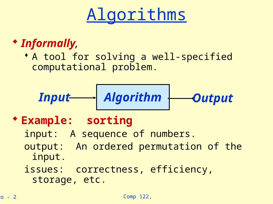
Algorithms

Informally, A tool for solving a well-specified computational

problem.

Example: sortinginput: A sequence of numbers.output: An ordered permutation of the input.issues: correctness, efficiency, storage, etc.

AlgorithmInput Output

Comp 122, Intro - 3

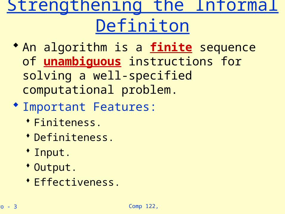
Strengthening the Informal Definiton

An algorithm is a finite sequence of unambiguous instructions for solving a well-specified computational problem.

Important Features: Finiteness. Definiteness. Input. Output. Effectiveness.

Comp 122, Intro - 4

Algorithm – In Formal Terms…

In terms of mathematical models of computational platforms (general-purpose computers).

One definition – Turing Machine that always halts. Other definitions are possible (e.g. Lambda Calculus.) Mathematical basis is necessary to answer questions

such as: Is a problem solvable? (Does an algorithm exist?) Complexity classes of problems. (Is an efficient algorithm

possible?)

Interested in learning more? Take COMP 181 and/or David Harel’s book Algorithmics.

Comp 122, Intro - 5

Algorithm Analysis Determining performance characteristics.

(Predicting the resource requirements.) Time, memory, communication bandwidth etc. Computation time (running time) is of primary

concern. Why analyze algorithms?

Choose the most efficient of several possible algorithms for the same problem.

Is the best possible running time for a problem reasonably finite for practical purposes?

Is the algorithm optimal (best in some sense)? – Is something better possible?

Comp 122, Intro - 6

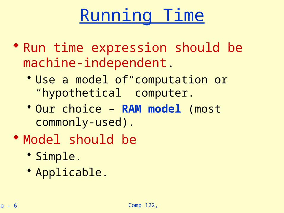
Running Time

Run time expression should be machine-independent. Use a model of computation or “hypothetical”

computer. Our choice – RAM model (most commonly-used).

Model should be Simple. Applicable.

Comp 122, Intro - 7

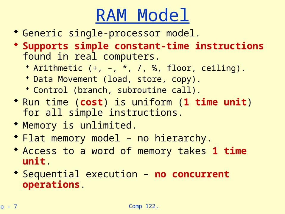
RAM Model Generic single-processor model. Supports simple constant-time instructions found in

real computers. Arithmetic (+, –, *, /, %, floor, ceiling). Data Movement (load, store, copy). Control (branch, subroutine call).

Run time (cost) is uniform (1 time unit) for all simple instructions.

Memory is unlimited. Flat memory model – no hierarchy. Access to a word of memory takes 1 time unit. Sequential execution – no concurrent operations.

Comp 122, Intro - 8

Model of Computation

Should be simple, or even simplistic. Assign uniform cost for all simple operations and

memory accesses. (Not true in practice.) Question: Is this OK?

Should be widely applicable. Can’t assume the model to support complex

operations. Ex: No SORT instruction. Size of a word of data is finite. Why?

Comp 122, Intro - 9

Running Time – Definition

Call each simple instruction and access to a word of memory a “primitive operation” or “step.”

Running time of an algorithm for a given input is The number of steps executed by the algorithm on

that input.

Often referred to as the complexity of the algorithm.

Comp 122, Intro - 10

Complexity and Input

Complexity of an algorithm generally depends on Size of input.

• Input size depends on the problem.– Examples: No. of items to be sorted.

– No. of vertices and edges in a graph.

Other characteristics of the input data.• Are the items already sorted?

• Are there cycles in the graph?

Comp 122, Intro - 11

Worst, Average, and Best-case Complexity Worst-case Complexity

Maximum steps the algorithm takes for any possible input.

Most tractable measure. Average-case Complexity

Average of the running times of all possible inputs. Demands a definition of probability of each input,

which is usually difficult to provide and to analyze. Best-case Complexity

Minimum number of steps for any possible input. Not a useful measure. Why?

Comp 122, Intro - 12

Pseudo-code Conventions

Read about pseudo-code in the text. pp 19 – 20. Indentation (for block structure). Value of loop counter variable upon loop termination. Conventions for compound data. Differs from syntax in

common programming languages. Call by value not reference. Local variables. Error handling is omitted. Concerns of software engineering ignored. …

Comp 122, Intro - 13

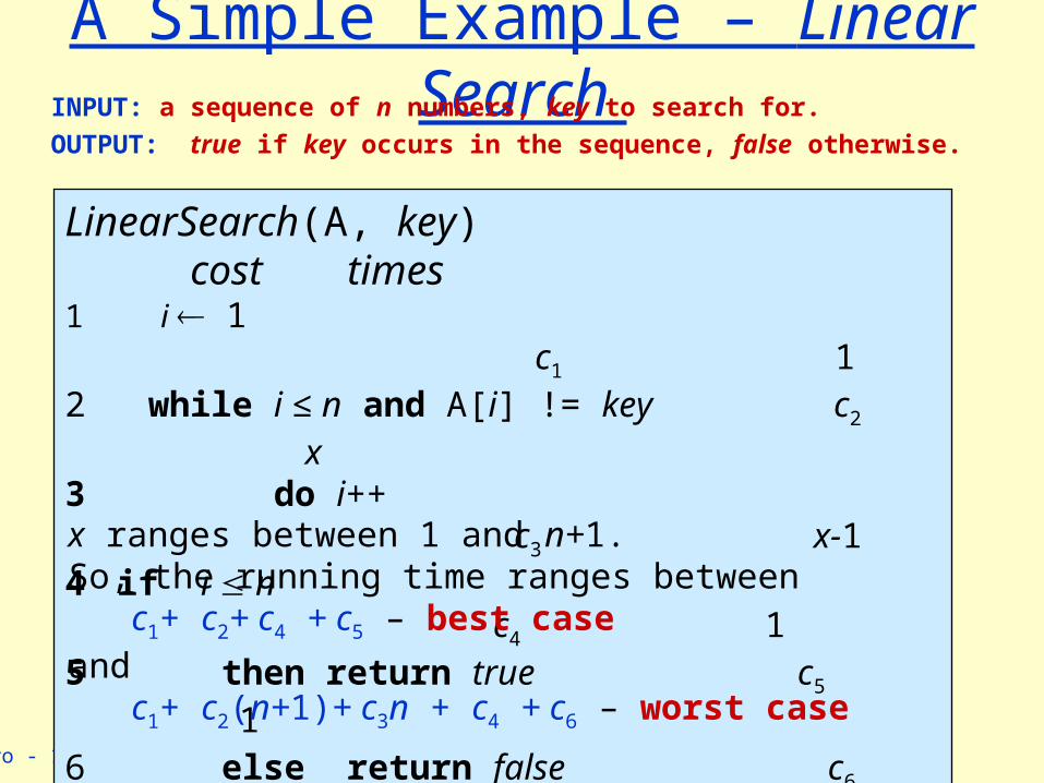
A Simple Example – Linear Search INPUT: a sequence of n numbers, key to search for.

OUTPUT: true if key occurs in the sequence, false otherwise.

n

i 21

LinearSearch(A, key) cost times1 i 1 c1 12 while i ≤ n and A[i] != key c2 x3 do i++ c3 x-14 if i n c4 15 then return true c5 16 else return false c6 1x ranges between 1 and n+1.So, the running time ranges between c1+ c2+ c4 + c5 – best caseand c1+ c2(n+1)+ c3n + c4 + c6 – worst case

Comp 122, Intro - 14

A Simple Example – Linear Search INPUT: a sequence of n numbers, key to search for.

OUTPUT: true if key occurs in the sequence, false otherwise.

n

i 21

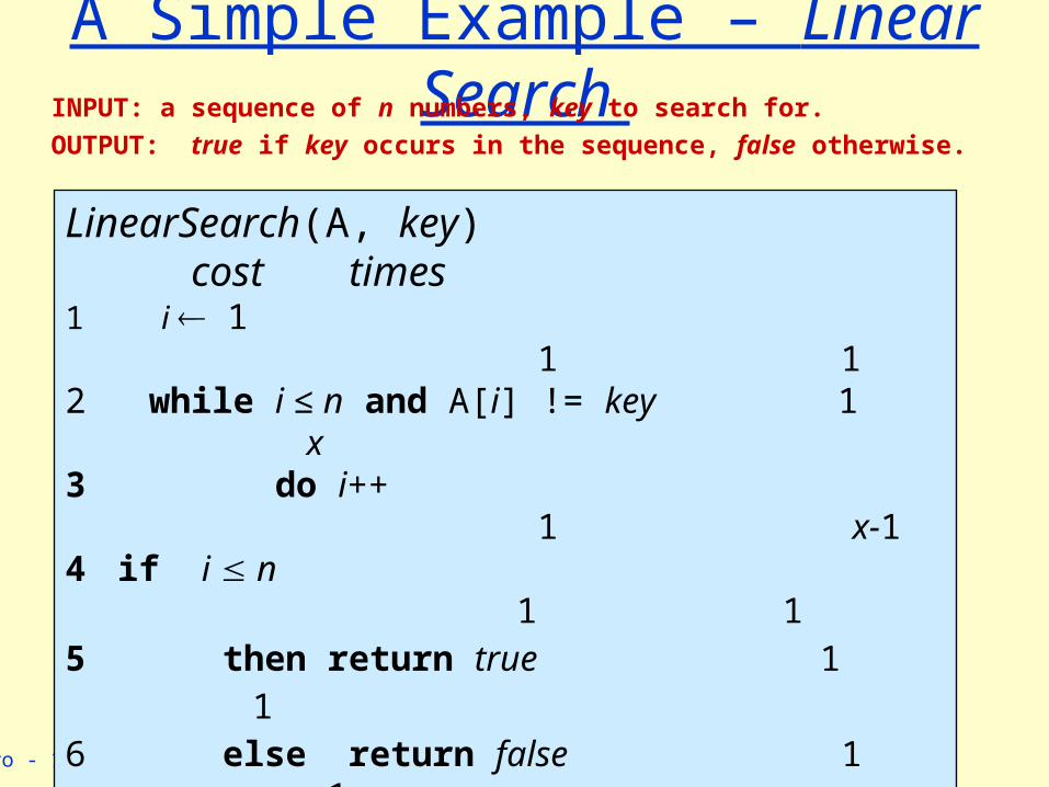
Assign a cost of 1 to all statement executions.Now, the running time ranges between 1+ 1+ 1 + 1 = 4 – best caseand 1+ (n+1)+ n + 1 + 1 = 2n+4 – worst case

LinearSearch(A, key) cost times1 i 1 1 12 while i ≤ n and A[i] != key 1 x3 do i++ 1 x-14 if i n 1 15 then return true 1 16 else return false 1 1

Comp 122, Intro - 15

A Simple Example – Linear Search INPUT: a sequence of n numbers, key to search for.

OUTPUT: true if key occurs in the sequence, false otherwise.

n

i 21

If we assume that we search for a random item in the list,on an average, Statements 2 and 3 will be executed n/2 times.Running times of other statements are independent of input.Hence, average-case complexity is 1+ n/2+ n/2 + 1 + 1 = n+3

LinearSearch(A, key) cost times1 i 1 1 12 while i ≤ n and A[i] != key 1 x3 do i++ 1 x-14 if i n 1 15 then return true 1 16 else return false 1 1

Comp 122, Intro - 16

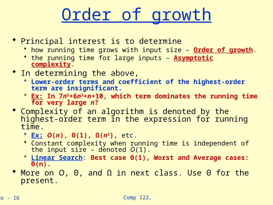
Order of growth Principal interest is to determine

how running time grows with input size – Order of growth. the running time for large inputs – Asymptotic complexity.

In determining the above, Lower-order terms and coefficient of the highest-order term are

insignificant. Ex: In 7n5+6n3+n+10, which term dominates the running time for

very large n? Complexity of an algorithm is denoted by the highest-order term

in the expression for running time. Ex: Ο(n), Θ(1), Ω(n2), etc. Constant complexity when running time is independent of the input size

– denoted Ο(1). Linear Search: Best case Θ(1), Worst and Average cases: Θ(n).

More on Ο, Θ, and Ω in next class. Use Θ for the present.

Comp 122, Intro - 17

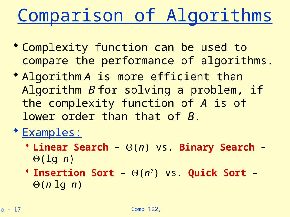
Comparison of Algorithms

Complexity function can be used to compare the performance of algorithms.

Algorithm A is more efficient than Algorithm B for solving a problem, if the complexity function of A is of lower order than that of B.

Examples: Linear Search – (n) vs. Binary Search – (lg n) Insertion Sort – (n2) vs. Quick Sort – (n lg n)

Comp 122, Intro - 18

Comparisons of Algorithms Multiplication

classical technique: O(nm) divide-and-conquer: O(nmln1.5) ~ O(nm0.59) For operands of size 1000, takes 40 & 15 seconds

respectively on a Cyber 835.

Sorting insertion sort: (n2) merge sort: (n lg n) For 106 numbers, it took 5.56 hrs on a

supercomputer using machine language and 16.67 min on a PC using C/C++.

Comp 122, Intro - 19

Why Order of Growth Matters? Computer speeds double every two years,

so why worry about algorithm speed? When speed doubles, what happens to the

amount of work you can do? What about the demands of applications?

Comp 122, Intro - 20

Effect of Faster Machines

• Higher gain with faster hardware for more efficient algorithm.

• Results are more dramatic for more higher speeds.

No. of items sorted

Ο(n2)

H/W SpeedComp. of Alg.

1 M* 2 M Gain

1000 1414 1.414

O(n lgn) 62700 118600 1.9

* Million operations per second.

Comp 122, Intro - 21

Correctness Proofs

Proving (beyond “any” doubt) that an algorithm is correct. Prove that the algorithm produces correct output

when it terminates. Partial Correctness. Prove that the algorithm will necessarily terminate.

Total Correctness. Techniques

Proof by Construction. Proof by Induction. Proof by Contradiction.

Comp 122, Intro - 22

Loop Invariant

Logical expression with the following properties. Holds true before the first iteration of the loop –

Initialization. If it is true before an iteration of the loop, it remains true

before the next iteration – Maintenance. When the loop terminates, the invariant ― along with the

fact that the loop terminated ― gives a useful property that helps show that the loop is correct – Termination.

Similar to mathematical induction. Are there differences?

Comp 122, Intro - 23

Correctness Proof of Linear Search

Use Loop Invariant for the while loop: At the start of each iteration of the while loop, the

search key is not in the subarray A[1..i-1].

LinearSearch(A, key)1 i 12 while i ≤ n and A[i] != key3 do i++4 if i n5 then return true6 else return false

If the algm. terminates, then it produces correct result.

Initialization.Maintenance.Termination.

Argue that it terminates.

Comp 122, Intro - 24

Go through correctness proof of insertion sort in the text.