What Happens When Wal-Mart Comes to Town: An

Empirical Analysis of the Discount Industry∗

Panle Jia†

JOB MARKET PAPER

Abstract

In the past few decades the retail industry has experienced substantial growth in multi-

store retailers, especially chains with a hundred or more stores. At the same time, there is

widely reported public outcry over the impact of these chain stores on small retailers and

local communities. This paper develops an empirical model to assess the impact of chain

stores on the profitability and entry/exit decisions of small retailers and to quantify the

size of the scale economies within a chain. The model has two key features. First, it allows

for fully flexible competition patterns among all players. Second, for chains, it incorporates

the scale economies that arise from operating multiple stores in nearby regions. In doing

so, the model relaxes the commonly used assumption that entry in different markets is

independent. The estimation exploits a unique data set that covers the discount retail

industry from 1988 to 1997. The results indicate that Wal-Mart’s expansion from the late

1980s to the late 1990s explains about fifty to seventy percent of the net change in the

number of small discount retailers. Failure to address the endogeneity of the firms’ entry

decisions results in underestimating this impact by fifty to sixty percent. Direct subsidies

to either chains or small retailers are unlikely to be cost effective in increasing the number

of firms or the level of employment. The Wal-Mart stores that received subsidies in the last

decade are on average more profitable than the unsubsidized ones. Finally, scale economies

were important in Wal-Mart’s early expansion period in the late 1980s, but their magnitude

diminished greatly in the late 1990s.

Keywords: Competition, Entry, Chain effect, Cross-sectional Dependence

JEL Classifications: L13, L81, L52, C13, C61

∗I am deeply indebted to my committee Steven Berry, Penny Goldberg, Hanming Fang, and Philip Haile for

their continual support and encouragement. Special thanks go to Pat Bayer, who has been very generous with

his help. I have also benefited from constructive discussions with Donald Andrews, Donald Brown, George Hall,

Judy Chevalier, Yuichi Kitamura, Alvin Klevorick, Herbert Scarf, and my colleagues at Yale University.†Department of Economics, Yale University. Email: panle.jia@yale.edu.

Contents

1 Introduction 1

2 Industry background 5

3 Data 6

3.1 Data sources . . . . . . . . . . . . . . . . . . . . . . . . . . . . . . . . . . . . . 6

3.2 Market definition and data description . . . . . . . . . . . . . . . . . . . . . . . 7

4 Modeling 9

4.1 Model setup . . . . . . . . . . . . . . . . . . . . . . . . . . . . . . . . . . . . . . 9

4.2 The profit function . . . . . . . . . . . . . . . . . . . . . . . . . . . . . . . . . . 10

4.3 Discussion . . . . . . . . . . . . . . . . . . . . . . . . . . . . . . . . . . . . . . . 13

4.3.1 Information structure . . . . . . . . . . . . . . . . . . . . . . . . . . . . 13

4.3.2 I.I.D. errors and the cross-sectional dependence arising from the chain

effect . . . . . . . . . . . . . . . . . . . . . . . . . . . . . . . . . . . . . . 14

4.3.3 Multiple equilibria . . . . . . . . . . . . . . . . . . . . . . . . . . . . . . 15

4.3.4 The symmetry assumption among small stores . . . . . . . . . . . . . . 15

5 Estimation 15

5.1 The chain’s single agent problem . . . . . . . . . . . . . . . . . . . . . . . . . . 16

5.2 The maximization problem with two competing chains . . . . . . . . . . . . . . 19

5.3 Adding small stores . . . . . . . . . . . . . . . . . . . . . . . . . . . . . . . . . 21

5.4 Further discussions . . . . . . . . . . . . . . . . . . . . . . . . . . . . . . . . . . 21

5.5 Empirical implementation . . . . . . . . . . . . . . . . . . . . . . . . . . . . . . 23

6 Results 25

6.1 Parameter Estimates . . . . . . . . . . . . . . . . . . . . . . . . . . . . . . . . . 25

6.2 The competition effect and the chain effect . . . . . . . . . . . . . . . . . . . . 27

6.3 The impact of Wal-Mart’s expansion and related policy issues . . . . . . . . . . 30

7 Conclusion and future work 33

8 Appendix: Definitions and Proofs 34

ii

“Bowman’s (in a small town in Georgia) is the eighth ‘main street’ business to close since

Wal-Mart came to town.. . . For the first time in seventy-three years the big corner store is

empty.” Archer and Taylor, Up against the Wal-Mart.

“There is ample evidence that a small business need not fail in the face of competition from

large discount stores. In fact, the presence of a large discount store usually acts as a magnet,

keeping local shoppers. . . .and expanding the market. . . .” Morrison Cain, Vice president of

International Mass Retail Association.

1 Introduction

The landscape of the U.S. retail industry has gone through considerable changes over the

past few decades, with two closely related trends. One is the rise of discount retailing; the

other is the increasing prevalence of large retail chains. In fact, the discount retailing sector

is almost entirely controlled by chains. In 1997, the top three chains (Wal-Mart, Kmart, and

Target) accounted for seventy-four percent of total sales and more than half of the discount

stores.

Discount retailing is a fairly new concept in the retail industry, with the first discount

stores appearing in the 1950s. The leading magazine for the discount industry, Discount

Merchandiser, defines a modern discount store as a departmentalized retail establishment that

makes use of self-service techniques to sell a large variety of hard goods and soft goods at

uniquely low margins.1 Over the span of several decades, the sector has emerged from the

fringe of the retail industry and become part of the mainstream. The total sales revenue of

discount stores, in real terms, increased about sixteen times from 1960 to 1997, compared to

less than threefold for the entire retail industry during the same period.

As the discount retailing sector continues to grow, opposition from other retailers, especially

small retailers, begins to mount. The critics tend to associate discounters and other big retailers

with small town problems caused by the closing of small stores, like the decline of downtown

shopping districts, eroded tax bases, decreased employment, and the disintegration of once

closely knitted communities.

Partly because tax money is used to restore the blighted downtown business districts and

to lure businesses from big retailers in various forms of economic development subsidies,2 the

1According to Annual Benchmark Report for Retail Trade and Food Services: January 1992 Through March

2002, published by the Census Bureau, the average markup for regular department stores was 27.9%, while the

average markup for discount stores was 20.9% from 1993 to 1997. Both markups went up slightly from 1998 to

2000.2See The Shils Report (1997): Measuring the Economic and Sociological Impact of the Mega-Retail Discount

1

effect of big retailers on small stores and local communities has become a matter of public

concern. Despite the large amount of media reports and public debate, there has been little

empirical work that directly examines how the entry of chain stores affects small retailers. The

first goal of this paper is to address this issue. Specifically, the paper quantifies the impact

of national discount chains on the profitability and entry and exit decisions of small retailers

from the late 1980s to the late 1990s.

As mentioned above, a prominent feature of the retail industry, including the discount

sector, is the increasing dominance of large chains in the past several decades. In 1997, retail

chains with a hundred or more stores accounted for less than one-tenth of a percent of the

total number of firms, yet they controlled twenty-one percent of the establishments, thirty-

seven percent of sales, and forty-six percent of the retail employment.3 Compared with the

late 1960s, their share of the retail market has more than doubled. In spite of the dominance

of chain stores, few empirical studies have tried to quantify the potential advantages of chains

over single unit firms (with the exception of Holmes (2005) and Smith (2004)),4 because of

the daunting complexities in modeling chain effects. In entry models, for example, the nature

of multi-unit chains implies that store entry decisions across markets are related. In contrast,

most existing literature has assumed that entry decisions are independent across markets and

has focused on competition among single-unit firms in local markets. The second goal of this

paper is to extend the entry literature by relaxing the independence assumption, and quantify

the chain effect by explicitly modeling chains’ entry decisions in a large number of markets.

My model has two key features. First, it allows for fully flexible competition patterns among

all retailers. Second, it relaxes the independent entry assumption and incorporates the potential

benefits of locating multiple stores in nearby regions; this is one of the major differences between

chain stores and single unit firms. Such benefits, which I call ‘the chain effect’ in this paper, can

arise through several different channels. For example, there may be significant scale economies

in the distribution system; stores close by can split the advertising costs or employee training

costs, or they can share knowledge about the specific features of the local markets. The chain

effect causes profits of the same-chain stores to be cross-sectionally dependent; as a result, the

profit maximization and location choices of chains become a complicated problem with a large

number of discrete choice variables, one for each market.

Instead of solving the problem directly, I transform it to a problem that searches for the

Chains on Small Enterprises in Urban, Suburban and Rural Communities.3See the 1997 Economic Census Retail Trade subject series Establishment and Firm Size (Including Legal

Form of Organization), published by US Census Bureau.4 I discuss Holmes (2005) in detail below. Smith (2004) estimates the demand cross-elasticities between stores

of the same firm and finds that mergers between the largest retail chains increase price level by up to 7.4%.

2

fixed points of the necessary conditions. Exploiting the features of the set of fixed points,

I propose a bound approach that facilitates the search for the optimal solution by reducing

the number of necessary computational evaluations from 22065 to a manageable number.5 In

analyzing the interaction of the chain effect with the competition effects, I take advantage of

the supermodular property of the profit functions.

The estimation exploits a unique data set I collected that covers the entire discount retail

industry from 1988 to 1997; during this period, the two major national chains were Wal-

Mart and Kmart.6 It explicitly addresses the issue of cross-sectional dependence using the

econometric technique proposed by Conley (1999). The simulation results indicate that Wal-

Mart’s expansion from the late 1980s to the late 1990s explains about fifty to seventy percent of

the net change in the number of small discount retailers. Unobserved market-level profit shocks

lead to a positive correlation between the entry decisions of chains and small stores; failure

to address this endogeneity issue results in underestimating the impact of Wal-Mart on small

stores by fifty to sixty percent. In addition, I find that government subsidies to either chains

or small firms in this industry are not likely to be cost effective in increasing the number of

firms or the level of employment. The Wal-Mart stores that have received subsidies from local

governments, of which there are publicly available records, are on average more profitable than

the unsubsidized ones. Last, scale economies were important in Wal-Mart’s early expansion

period in the late 1980s, but their impact diminished greatly in the late 1990s.

The paper complements a recent study by Holmes (2005), which analyzes the diffusion

process of Wal-Mart stores in the last several decades to quantify the economies of density,

defined as the cost savings from locating stores close to each other. The concept of economies

of density is similar to the chain effect in this paper. The central insight in his paper is that

markets vary in quality; in the absence of the economies of density, Wal-Mart would open

stores in the most profitable markets first, and gradually expand to less profitable markets.

Since profitable markets do not necessarily cluster, one should observe Wal-Mart open stores

sporadically across regions. The actual opening process, however, displayed a regular diffusion

pattern from the South, where Wal-Mart’s headquarters are, to other regions. Due to the

complexity of the dynamics (the state space grows exponentially with the number of markets),

it is infeasible to solve Wal-Mart’s optimization problem. The paper adopts a perturbation

approach to estimate the economies of density. The findings suggest that the benefit of the

5There are 2065 markets in the sample. With two choices for each market (enter or stay outside the market),

22065 is the number of possible location choices for each chain.6During the sample period, Target is a regional store that competes mostly in the big metropolitan areas in

the Midwest with few stores in the sample. See the data section for more details.

3

economies of density is sizable.

An appealing feature of the Holmes’ approach is that the size of the economies of density

is derived from the dynamic expansion process. In contrast, the chain effect in my paper is

identified from the stores’ geographic clustering pattern and depends on the model’s equilib-

rium assumption. The disadvantage of my approach is that it abstracts from many dynamic

considerations. For example, it does not allow firms to delay store openings because of credit

constraints. Neither does it allow for any preemption motives (the chains compete and make

entry decisions simultaneously). Ideally, one would like to develop and estimate a dynamic

model that incorporates both the competition effects and the economies of density. However,

given that it is very difficult to estimate the economies of density in a single agent dynamic

model as is shown in Holmes (2005), it is clearly infeasible to estimate a model that also incor-

porates the strategic interactions within chains and between chains and small retailers. Since

the goal of this paper is to analyze the competition effects and perform policy evaluations, I

adopt a simple two-stage model where all players make a once-and-for-all decision, with chains

moving first and small retailers moving second. The extension of the current framework to a

dynamic model is left for future research.

This paper relates to a large literature on spatial competition in the retail markets, for

example, Pinkse et. al. (2002), Smith (2004), and Davis (2005). All of these models take the

firms’ locations as given and focus on the price or quantity competition. I adopt the opposite

approach. Specifically, I assume a parametric form for the firms’ reduced-form profit functions

from the stage competition, and focus on how they compete spatially by balancing the market

size consideration with the competition effect of rivals’ actions on their own profits.

To the extent that retail chains can be treated as multi-product firms whose differentiated

products are stores with different locations, this paper is also related to several recent empirical

entry papers that endogenize firms’ product choices upon entry. For example, Mazzeo (2002)

studies the quality choices of highway motels. Seim (2005) studies how video stores soften the

competition by choosing different locations. Unlike these studies, in which each firm chooses

only one product, this paper focuses on the behavior of multi-product firms whose product

spaces are potentially large.

The paper also contributes to the growing literature on Wal-Mart, which includes Stone’s

(1995) study of Wal-Mart’s impact on small towns in Iowa and Basker’s (2005) study of the

labor market effects of Wal-Mart’s expansion. These papers focus exclusively on Wal-Mart,

while my paper also incorporates Wal-Mart’s rivals.

The remainder of the paper is structured as follows. Section 2 provides some additional

background information regarding this industry. Section 3 describes the data set. Section 4

4

discusses the model. Section 5 proposes an estimation method to deal with the complicated

optimization problem faced by a chain in the presence of rival retailers. Section 6 presents the

results. Section 7 concludes. The appendix fills in the technical details not covered in section

5.

2 Industry background

Ever since its inception, discount retailing has been one of the most dynamic sectors in

the retail industry. The sales revenue for this sector, in 2004 US dollars, has skyrocketed from

thirteen billion in 1960 to around two hundred billion in 1997. In comparison, the sales revenue

for the entire retail industry has only achieved a modest increase from around five hundred

billion to thirteen hundred billion during the same period. The number of discount stores

has multiplied from thirteen hundred to almost ten thousand, while the number of firms has

dropped from a thousand to two hundred and thirty. Table 1 displays some statistics for the

industry from 1960 to 1997.

Like the other retail sectors, the discount industry is dominated by chain stores. In 1970,

thirty-nine discount chains with twenty-five or more stores each operated roughly half of the

discount stores and accounted for forty percent of total sales. In 1989, both shares increased

to roughly eighty-five percent. By the late 1990s, the twenty-eight firms with twenty-five or

more stores controlled roughly ninety-four percent of total stores and sales.

Many reasons have been suggested for the success of chains. The principal advantages

of chain stores include the ability of the central purchasing unit to buy on favorable terms

and to foster specialized buying skills; the possibility to split operating and advertising cost

among multiple units; and the freedom to experiment in one selling unit without risk to the

whole operation. Stores also frequently share their private information of the local markets

and learn from each other’s managerial practices. Finally, chains can achieve economies of

scale by combining wholesaling and retailing operations within the same business unit.

Until the late 1990s, two most important national chains were Kmart and Wal-Mart. Both

firms opened their first store in 1962. The first Kmart was opened by the variety-chain Kresge.

Kmart stores were a new experiment that provided consumers with quality merchandise at

prices considerably lower than those of regular retail stores. These stores emphasized nation-

ally advertised brand-name products to reduce advertising costs and to minimize customer

service. Consumer satisfaction was guaranteed and all goods could be returned for a refund

or an exchange (See Vance and Scott (1994), pp32). These practices were an instant success

and Kmart grew rapidly in the 1970s and 1980s. By the early 1990s, the firm had more than

5

twenty-two hundred stores nationwide. In the late 1980s, Kmart tried to diversify its business

and pursued various forms of specialty retailing in the areas of pharmaceutical products, sport-

ing goods, office supplies, building materials, etc. The attempt was unsuccessful and Kmart

eventually divested itself of these interests by the late 1990s. Struggling with its management

failures throughout the 1990s, Kmart maintained roughly the same number of stores, with

opening of new stores offset by the closing of existing ones.

Unlike Kmart, which was initially supported by an established retail firm, Wal-Mart started

from scratch and grew relatively slowly in the beginning. To avoid direct competition with

other discounters, it focused on small towns in the southern states where there were few

competitors. Starting from the early 1980s, the firm began its aggressive expansion process

that averaged a hundred and forty store openings per year. In 1991, Wal-Mart replaced Kmart

as the largest discounter. By 1997, Wal-Mart had about twenty-four hundred stores (not

including the wholesale clubs) in all states, including Alaska and Hawaii.

As the discounters continue to grow, small retailers start to feel their impact. There

are extensive media reports on the controversies associated with the impact of large chains

on small retailers, and on local communities in general. In 1994, the United States House

of Representatives convened a hearing titled “The Impact of Discount Superstores on Small

Businesses and Local Communities”. Witnesses from mass retail associations and small retail

councils testified, but no legislation followed, due to the lack of concrete evidence.

3 Data

Before introducing the model, I first discuss the data sets, as they dictate the modeling

approach used in this paper.

3.1 Data sources

There are four main data sources. The data set on discount chains comes from the annual

directories published by Chain Store Guide Inc. The directory covers all of the discount stores

with a footage of more than ten thousand square feet in operation during each year. For each

store, the directory lists its name, size, street address, telephone number, store format, and

firm affiliation.7 The U.S. industry classification system changed from the Standard Industrial

Classification System (SIC) to the North American Industry Classification System (NAICS) in

7The directory stopped providing store size information in 1997 and changed the inclusion criterion to 20,000

square feet in 1998. The store formats include membership stores, regional offices, and in later years distribution

centers.

6

1998. To avoid potential inconsistencies in the industry definition, I restrict the sample period

to the ten years before the classification change.

The second data set, the County Business Pattern, tabulates at the county level the number

of establishments by the size category for very detailed industry classifications. However, dis-

aggregated data at the three-digit or finer SIC levels are unusable because of data suppression

due to confidentiality requirements.8 There are eight retail sectors at the two-digit SIC level:

building materials and garden supplies, general merchandise stores, food stores, automotive

dealers and service stations, apparel and accessory stores, furniture and home-furnishing stores,

eating and drinking places, and miscellaneous retail. The focus of this study is on small general

merchandise stores with nineteen or fewer employees, which are the direct competitors of the

discount chains. From a policy point of view, it is important to include a broader collection

of small retailers that are all affected by discount chains, for example, hardware stores, auto-

parts stores, or apparel stores. I am currently working on expanding the current specification

to include more categories of small retailers. The new results will be incorporated into this

paper once they are available.

County level population before 1990 and after 1990 is downloaded from the websites of

U.S. Census Bureau and the Missouri State Census Data Center, respectively. Other county

level demographic and retail sales data are from various years of the decennial census and

the economic census. Finally, the data on subsidized Wal-Mart stores that I exploit in a

simulation exercise come from an extensive study conducted and posted online by Good Jobs

First, a non-profit research institute based in Washington D.C.

3.2 Market definition and data description

In this paper, a market is defined as a county. Although the discount store data is at the

zip code level, information for small stores is at the county level. Many of the market size

variables, like retail sales, are also available only at the county level.

I focus on counties with an average population between five and sixty-four thousand from

1988 to 1997. There are 2065 such counties among a total of 3140 counties. According to

Vance and Scott (1994), the minimum county population for a Wal-Mart store is five thousand

in the 1980s, while Kmart concentrates on places with a much larger population. Nine percent

of the counties have five thousand or fewer people and are unlikely to be a potential market for

8Title 13 of the United States Code authorizes the Census Bureau to conduct censuses and surveys. Section

9 of the same Title requires that any information collected from the public under the authority of Title 13 be

maintained as confidential and no estimates are published that would disclose the operations of an individual

firm.

7

either chains. Twenty five percent of the counties are large metropolitan areas with an average

population of sixty-four thousand or more. They typically include multiple self-contained

shopping areas, and consumers are unlikely to travel across the entire county to shop. The

market configuration in these big counties tends to be very complex with a large number of

competitors and many market niches. For example, in the early 1990s, there were more than

one hundred big discounters and close to four hundred small general merchandise stores in Los

Angeles county, one of the largest counties. To capture the firms’ strategic behaviors in these

markets, one needs more detailed geographic information than the county level data.

During the sample period, there are two national chains: Kmart and Wal-Mart. The third

largest chain, Target, has three hundred forty stores in 1988 and about eight hundred stores

in 1997. Most of them are located in the metropolitan areas in the Midwest, with on average

less than twenty stores in the counties studied here. I do not include Target in the analysis.9

In the sample, only eight counties have two Kmart stores and forty-nine counties have two

Wal-Mart stores in 1988; the figures are eight and sixty-six counties in 1997, respectively. The

current specification abstracts from the store number choice and only considers the chains’

entry decisions for each market. In a robustness exercise, I allow Wal-Mart to choose whether

to open one store or two stores upon entry in each local market. The profit for the second

store is not precisely estimated, but other estimates do not change.

Table 2 presents summary statistics for the sample for the years 1988 and 1997. The

average population grows from twenty-two thousand to twenty-four thousand, an increase of

eight percent. Retail sales per capita, in 1984 dollars, rise ten percent, from thirty-seven

hundred to forty-one hundred. The average percentage of urban population is thirty percent

in 1988 and increases to thirty-three percent in 1997. About one quarter of the counties are

primarily rural with very little urban population, which is why the average across the counties

seems somewhat low. About forty percent of the counties are in the Midwest (including the

Grate Lakes region, the Plains region, and the Rocky Mountain region, as defined by the

Bureau of Economic Analysis), and another fifty percent of the counties lie in the southern

regions (including the Southeast region and the Southwest region), with the rest in the Far

West and the Northeast region. Twenty-one percent of the counties have Kmart stores at

the beginning of the sample period and the number drops slightly to nineteen percent at the

end. In comparison, Wal-Mart has stores in thirty-four percent of the counties in 1988, and

fifty-one percent in 1997.10 The average number of small stores decreases quite a bit over the

9The rest of the discount chains are much smaller and are all regional. They are not included in the analysis.10There are 433 and 393 counties with Kmart stores in 1988 and 1997, and 660 and 982 counties with Wal-Mart

stores in 1988 and 1997, respectively.

8

same period, from 3.86 to 3.49. The median is three, with a maximum of twenty-five small

stores in 1987, and nineteen in 1997. The percentage of counties with six or more small stores

drops from twenty-two percent to eighteen percent, while the percentage of counties with at

most one small store increases from eighteen percent to twenty-two percent over the sample

period.

4 Modeling

4.1 Model setup

The model I develop is a two-stage game with complete information. In stage one, Kmart

and Wal-Mart simultaneously choose store locations to maximize their total profits in all

markets. In stage two, small firms observe Kmart and Wal-Mart’s choices and decide whether

to enter the market.11 Once the entry decisions are made, firms compete and profits are

realized. All firms have perfect knowledge of rivals’ profitability, are fully rational and know

their payoff structures. When Kmart and Wal-Mart make location choices in the first stage,

they take into consideration the reaction from the small retailers. There are no entry barriers;

small firms enter the market until profit for an extra entrant becomes negative.

In reality, small retailers have existed long before the era of the discount chains. As the

chains emerge in the retail industry, small stores either continue their operations and compete

with the chains or exit the market entirely. Perhaps a better approach would be a three-

stage model, with each stage corresponding to each of these events. However, if one assumes

that small firms lack the ability to make credible commitments, that is, they can’t credibly

claim to stay in the market even if the business is failing as big chains enter, the two-stage

model produces the same predictions as the three-stage model. Given their lack of access to

the capital market, small retailers are unlikely to linger on when the store is not profitable.

Indeed, The Shils report (1997), a survey conducted by Edward B. Shils, shows that a small

store typically closes down within six to twelve months in the face of a failing business. In

contrast, I have implicitly assumed that chains can commit to their first-stage entry decisions

and do not further adjust after small stores enter. This is based on the observation that most

of the chain stores enter with a long-term lease of the rental property, and in many cases invest

considerably in the infrastructure construction associated with establishing a big store.

11 I have implicitly assumed that small stores, which are stores with one to nineteen employees, are single-unit

stores.

9

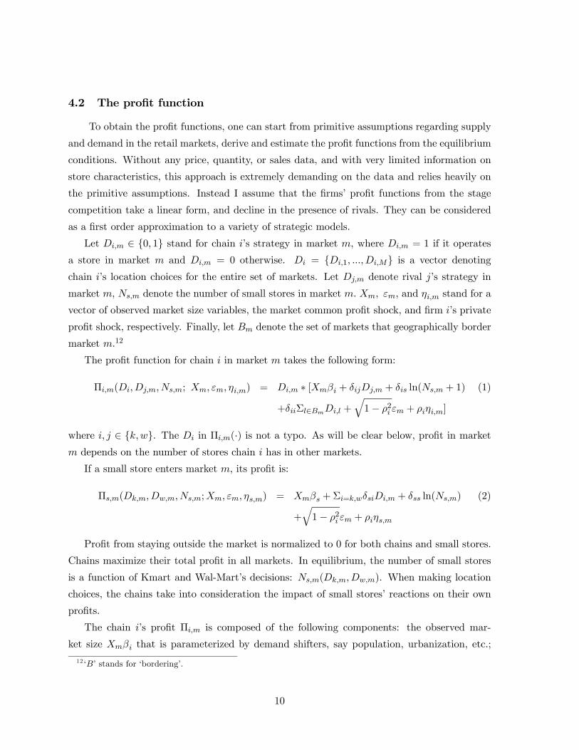
4.2 The profit function

To obtain the profit functions, one can start from primitive assumptions regarding supply

and demand in the retail markets, derive and estimate the profit functions from the equilibrium

conditions. Without any price, quantity, or sales data, and with very limited information on

store characteristics, this approach is extremely demanding on the data and relies heavily on

the primitive assumptions. Instead I assume that the firms’ profit functions from the stage

competition take a linear form, and decline in the presence of rivals. They can be considered

as a first order approximation to a variety of strategic models.

Let Di,m ∈ 0, 1 stand for chain i’s strategy in market m, where Di,m = 1 if it operates

a store in market m and Di,m = 0 otherwise. Di = Di,1, ...,Di,M is a vector denotingchain i’s location choices for the entire set of markets. Let Dj,m denote rival j’s strategy in

market m, Ns,m denote the number of small stores in market m. Xm, εm, and ηi,m stand for a

vector of observed market size variables, the market common profit shock, and firm i’s private

profit shock, respectively. Finally, let Bm denote the set of markets that geographically border

market m.12

The profit function for chain i in market m takes the following form:

Πi,m(Di,Dj,m, Ns,m; Xm, εm, ηi,m) = Di,m ∗ [Xmβi + δijDj,m + δis ln(Ns,m + 1) (1)

+δiiΣl∈BmDi,l +q1− ρ2i εm + ρiηi,m]

where i, j ∈ k,w. The Di in Πi,m(·) is not a typo. As will be clear below, profit in marketm depends on the number of stores chain i has in other markets.

If a small store enters market m, its profit is:

Πs,m(Dk,m,Dw,m, Ns,m;Xm, εm, ηs,m) = Xmβs +Σi=k,wδsiDi,m + δss ln(Ns,m) (2)

+q1− ρ2i εm + ρiηs,m

Profit from staying outside the market is normalized to 0 for both chains and small stores.

Chains maximize their total profit in all markets. In equilibrium, the number of small stores

is a function of Kmart and Wal-Mart’s decisions: Ns,m(Dk,m,Dw,m). When making location

choices, the chains take into consideration the impact of small stores’ reactions on their own

profits.

The chain i’s profit Πi,m is composed of the following components: the observed mar-

ket size Xmβi that is parameterized by demand shifters, say population, urbanization, etc.;

12 ‘B’ stands for ‘bordering’.

10

the unobserved profit shockq1− ρ2i εm + ρiηi,m, known to the firms but unobserved by the

econometrician; the competition effect δijDj,m + δis ln(Ns,m + 1), as well as the chain effect

δiiΣl∈BmDi,l. Notice that the observed market size component Xmβi is allowed to be different

for different players. Xm includes all factors that influence profit, and βi is firm specific and

picks up the factors that are relevant for player i. For example, Kmart might have some ad-

vantage in the Midwestern region, while Wal-Mart stores might be more profitable in markets

close to their headquarters.

The unobserved profit shock has two elements:q1− ρ2i εm (with 0 ≤ ρi ≤ 1), where εm

is the market-level profit shifter that affects both chains and small stores, and ρiηi,m, a firm

specific profit shock. εm is assumed to be i.i.d. across markets, while ηi,m is assumed to be

i.i.d. across firms and markets.q1− ρ2i measures how important the market component is to

player i and can be different for chains and small stores. For example, the market specific busi-

ness environment — how developed the infrastructure is, whether the market has sophisticated

shopping facilities, and the stance of the local community toward large corporations including

big retailers — might matter more to chains than to small stores. In the baseline specification,

I restrict ρs = ρk = ρw. Relaxing it does not seem to improve the fit much.13 ηi,m incorporates

the unobserved firm heterogeneity, including the management ability, store display style, store

shopping environment, employees’ morale or skills, etc., that differ from store to store. As is

standard in discrete choice models, the scale of the parameter coefficients and the variance of

the error term are not separately identified. I normalize the variance of the error term to one

by assuming that both εm and ηi,m are standard normal random variables.

The competition effect from the rival chain is captured by δijDj,m, where Dj,m is one if

there is a store operated by rival j in market m. δis ln(Ns,m + 1) denotes the effect of small

stores on chain i’s profit. The addition of 1 in ln(Ns,m + 1) is used to avoid ln 0 for markets

without any small stores. The log form allows the incremental competition effect to taper off

when there are many small stores.

The last term in the bracket δiiΣl∈BmDi,l captures the chain effect. δii is assumed to

be non-negative. Bm is the set of markets that are adjacent to market m, and δiiΣl∈BmDi,l

is the benefit of having stores in the adjacent markets on the profitability in market m. As

mentioned in the introduction, chains can split the operation cost, delivery cost, and advertising

cost among nearby stores to achieve the scale economies. They can also share knowledge of

the localized markets and learn from each other’s managerial success. All these factors suggest

13Besides the small difference in the minimized function values when allowing ρs to be different from ρk and

ρw, it is not clear where the identification comes from in this particular model.

11

that having stores nearby benefits the operation in market m, and vice versa. There are other

kinds of scale economies, for example, the scale economies that arise from a chain’s ability to

buy a large volume at a discount. It implies that opening a store in market m benefits all

stores, not just neighboring stores. However, to the extent that this type of scale economies

affect all stores by the same magnitude, it can’t be separately identified from the constant of

the profit function. The estimated chain effect, δii, should therefore be interpreted as a lower

bound to the actual benefits enjoyed by a chain.

The presence of the common market-level error term εm makes the number of big stores

(small stores) endogenous in the profit function of small (big) firms, since a large εm leads to

more entry from both chains and small stores. If one only wants to estimate the competition

effect of big retailers on small stores δsi, without analyzing the equilibrium consequences of

policy changes, it suffices to regress the number of small stores on market size variables,

together with the number of big stores, and use instruments to correct the OLS bias of the

competition effects. However, valid instruments for each of the rivals may be difficult to

find. Furthermore, the predicted number of small stores from this IV regression is not an

integer and can be negative. The limited dependent variable estimation avoids this awkward

feature, but accounting for endogeneity in the discrete games involves strong assumptions on

the nature of the endogeneity that are not satisfied by the current model. In contrast, this

paper explicitly addresses the issue of endogeneity by solving chains’ and small stores’ entry

decisions simultaneously within the model.

All small stores are symmetric with the same profit function Πs,m(·). For markets withno small stores, the entry condition requires that profit for a single small store is negative,

that is, Xmβs + Σi=k,wδsiDi,m +q1− ρ2i εm + ρiηs,m < 0. For markets with Ns,m stores,

Πs,m(Ns,m) ≥ 0 and Πs,m(Ns,m + 1) < 0. δss ln(Ns,m) captures the competition among small

stores, while Σi=k,wδsiDi,m denotes the impact of Kmart and Wal-Mart. The static nature

of the model does not allow separate identification of the different channels through which

competition effect takes place. For example, one can’t tell whether it leads to exit of small

stores, or it occurs via preemption that reduces entry by small stores.

Note that the above specification allows fully flexible competition patterns, with all the

possible firm-pair combinations. The focus of the estimation is on the competition effects

δij , i, j = k,w, s, i 6= j and the chain effects: δii, i = k,w.

12

4.3 Discussion

Several assumptions and caveats of the model are worth mentioning. In the following, I

discuss the game’s information structure, the independent error assumption, issues of multiple

equilibria, and the symmetry assumption for small stores.

4.3.1 Information structure

In the empirical I.O. literature, there have been several different modeling approaches in

studying static entry models. A common approach is to assume complete information and si-

multaneous entry. One problem with this approach is the presence of multiple equilibria, which

has posed considerable challenges to estimation. The presence of multiple equilibria makes the

direct application of the traditional Maximum Likelihood Estimator (MLE) problematic, since

MLE requires a one-to-one mapping between regions of the unobservables (model predicted

probabilities) and the observed equilibrium outcomes. Some authors look for features that

are common among different equilibria (for example, although the firm identities might differ

across different equilibria, the number of entering firms might be the same), like Bresnahan

and Reiss (1990 and 1991) and Berry (1992). Arguably, grouping different equilibria by their

common features leads to a loss of information and less efficient estimates. Further, common

features are increasingly difficult to find when the model becomes more realistic. Others give

up the point identification of parameters and search for bounds, hoping that the bounds can

still produce useful policy guidance, as in Andrews, Berry and Jia (2004), Chernozhukov, Hong,

and Tamer (2004), and Pakes, Porter, Ho, and Ishii (2005). However, a meaningful boundary

might be difficult to obtain in complicated models, as the one employed here that involves

three sets of profit functions with twenty-six parameters.

In some cases, the specific application suggests factors that favor a certain equilibrium.

For example, Berry (1992) shows that it might be reasonable to choose the equilibrium that

favors the most profitable firms. Bajari, Hong and Ryan (2004) formally model the equilibrium

selection rule by computing all possible equilibria and assuming that an equilibrium is more

likely if it is either trembling-hand perfect, in pure strategies, or maximizing the industry

profit. Their approach is fairly flexible and can be applied to a wide range of games with

reasonable complexities, but is computational infeasible in large games, due to the burden of

computing all the equilibria.

Seim (2004) takes a different approach and adopts an incomplete information framework,

where firms’ profit shocks ηi,m are private information. Her approach smooths moment condi-

tions and produces equality constraints, but it does not solve the problem of multiple equilibria

13

— there can be multiple vectors of firms’ beliefs that are consistent with the model. Another

concern with the incomplete information approach is that it leads to post-entry regret, which

might seem unsatisfactory given that the entry decision in these static models is a once-and-

for-all choice.

Given the above considerations, I adopt the complete-information framework and choose

an equilibrium that seems reasonable a priori. Computing all the equilibria is not feasible,

both because the number of possible equilibria is large (the maximum number is 2M), and

because finding an equilibrium is by no means trivial. As a robustness check, I estimate the

model using three sets of very different equilibria, and show that the results are robust to the

equilibrium choice.

4.3.2 I.I.D. errors and the cross-sectional dependence arising from the chain effect

As mentioned above, the demand shocks in the profit functions are assumed to be inde-

pendent across markets, an assumption commonly used in empirical models. The econometric

technique proposed by Conley (1999) can address a general pattern of cross-sectional depen-

dence among the error terms. Allowing dependent errors raises two difficulties. First, the

simulation method used in this paper requires detailed knowledge of the nature of the cross

sectional dependence among the error terms, which is hard to obtain.

The second, and a more fundamental difficulty, relates to the identification of the chain

effect. Recall that the chain effect is identified from the geographical clustering of the discount

stores, which can also be driven by the cross-sectional correlation of the demand errors. The

data at hand can’t separate these two possible explanations. However, with appropriate ex-

periments, for example an external shock that changes the cost of operating stores but does

not affect the nature of local demand, the chain effect can be separately identified from the

demand correlation. More specifically, suppose there are two adjacent markets, and the local

government in one market raises taxes or requires firms to comply with certain regulations that

increases their operating costs. If the policy change induces reduced entry in both markets,

one can conclude that chain effect exists. In the result section, I discuss evidence that the

estimated chain effect is mostly likely to be firm specific, rather than demand driven.

The chain effect causes store profit across markets to be related, which leads to the cross-

sectional dependence among the observed store entry decisions, even with the assumption of

independent error terms. For example, Wal-Mart store’s entry decision in Benton County, AR

directly relates to Wal-Mart store’s entry decision in Carroll County, AR., Benton’s neighbor.

Not only is Di,m correlated with Di,l for l ∈ Bm, Di,m is weakly correlated with any Di,k

14

if market m and market k are connected through one or more neighbors. The next section

explains in detail how the cross-sectional dependence can be incorporated in the estimation.

4.3.3 Multiple equilibria

As is common in most static entry models, there are multiple equilibria in this model. In

the case of simultaneous entry with two players and one market, there is a range of market

sizes that accommodates two equilibria: either player can profitably enter the market, but not

both. In the current application, there may be as many as 2M possible equilibria for some

parameter values (as is the case when δii = 0), where M is the number of markets. In the

baseline specification, I estimate the model using the equilibrium that is most profitable for

Kmart, which is motivated by the observation that Kmart comes from a much older entity

and historically had the first mover advantage. I then experiment with two other cases. The

first one selects the equilibrium that assumes Kmart has advantage in the northern regions

while Wal-Mart has expertise in serving the southern regions. The second one chooses the

equilibrium that is most profitable for Wal-Mart. This is the extreme opposite to the baseline

specification.

4.3.4 The symmetry assumption among small stores

I have assumed that all small firms are symmetric with the same profit function. The

assumption is constrained by the data availability, as I do not observe any firm characteristics

for small stores. In practice, doing so greatly simplifies the complexity of the model with

asymmetric competition effects, as it guarantees that in the second stage the equilibrium

number of small stores in each market is unique.

5 Estimation

The unobserved market level profit shock εm, together with the chain effect Σl∈BmDi,l,

renders all of the discrete variables Di,m, Dj,m, Di,l, and Ns,m endogenous in the profit

functions (1) and (2). There are no closed form solutions to firms’ entry decisions and location

choices conditioning on the market size observables and a given vector of the parameter values.

I follow the method of simulated moments that has been widely used in the estimation of

structural models. Sections 5.1 - 5.4 explain in detail the algorithm I have developed to solve

the game for all of the players. Section 5.5 discusses the econometric tools and the moments

exploited in the estimation.

15

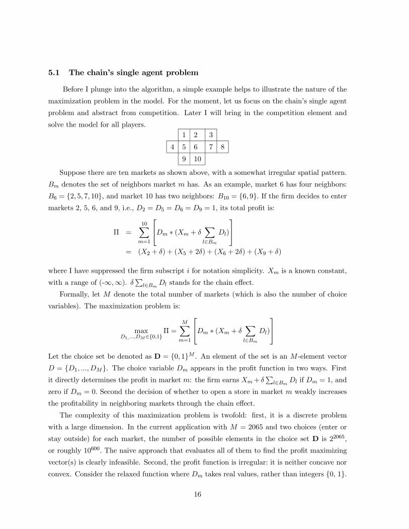
5.1 The chain’s single agent problem

Before I plunge into the algorithm, a simple example helps to illustrate the nature of the

maximization problem in the model. For the moment, let us focus on the chain’s single agent

problem and abstract from competition. Later I will bring in the competition element and

solve the model for all players.1 2 3

4 5 6 7 8

9 10

Suppose there are ten markets as shown above, with a somewhat irregular spatial pattern.

Bm denotes the set of neighbors market m has. As an example, market 6 has four neighbors:

B6 = 2, 5, 7, 10, and market 10 has two neighbors: B10 = 6, 9. If the firm decides to enter

markets 2, 5, 6, and 9, i.e., D2 = D5 = D6 = D9 = 1, its total profit is:

Π =10X

m=1

⎡⎣Dm ∗ (Xm + δXl∈Bm

Dl)

⎤⎦= (X2 + δ) + (X5 + 2δ) + (X6 + 2δ) + (X9 + δ)

where I have suppressed the firm subscript i for notation simplicity. Xm is a known constant,

with a range of (-∞,∞). δP

l∈BmDl stands for the chain effect.

Formally, let M denote the total number of markets (which is also the number of choice

variables). The maximization problem is:

maxD1,...,DM∈0,1

Π =MX

m=1

⎡⎣Dm ∗ (Xm + δXl∈Bm

Dl)

⎤⎦Let the choice set be denoted as D = 0, 1M . An element of the set is an M -element vector

D = D1, ...,DM. The choice variable Dm appears in the profit function in two ways. First

it directly determines the profit in market m: the firm earns Xm+ δP

l∈BmDl if Dm = 1, and

zero if Dm = 0. Second the decision of whether to open a store in market m weakly increases

the profitability in neighboring markets through the chain effect.

The complexity of this maximization problem is twofold: first, it is a discrete problem

with a large dimension. In the current application with M = 2065 and two choices (enter or

stay outside) for each market, the number of possible elements in the choice set D is 22065,

or roughly 10600. The naive approach that evaluates all of them to find the profit maximizing

vector(s) is clearly infeasible. Second, the profit function is irregular: it is neither concave nor

convex. Consider the relaxed function where Dm takes real values, rather than integers 0, 1.

16

The Hessian of this function is indefinite, and the usual first-order condition does not apply.

Even if one can exploit the first-order condition, the search with a large number of choice

variables is a daunting task.

Instead of solving the problem directly, I transform the problem into one that searches for

the fixed points of the necessary conditions. In particular, I exploit the feature of the set of

fixed points and propose an algorithm that obtains an upper bound DU and a lower bound

DL to the profit maximizing vector(s).With these two bounds at hand, I then evaluate all the

vectors that lie between them to find the profit maximizing vector(s).

It is possible that the set of profit maximizing vector is not a singleton. For example, in the

case of two markets with X1 = −1,X2 = −1, and δ = 1, both D∗ = 0, 0 and D∗∗ = 1, 1maximize the total profit. Here I assume there is only one optimal solution to the maximization

problem. In the appendix, I exploit two properties of the supermodular functions to show that

allowing multiple optimal solutions is a straightforward extension.

In the following discussion, the comparison between vectors is operated element by element.

A vector D is bigger than vector D0 iff every element of D is weakly bigger: D ≥ D0 iff

Dm ≥ D0m ∀m. D and D0 are unordered if neither D ≥ D0 nor D ≤ D0. They are the same if

both D ≥ D0 and D ≤ D0.

Let the profit maximizer be denoted as D∗ = argmaxD∈DΠ(D). The optimality of D∗

implies a set of necessary conditions:

Π(D∗1, ...,D∗m, ...,D

∗M) ≥ Π(D∗1, ...,Dm, ...,D

∗M),∀m

which implies:

D∗m = 1[Xm + 2δXl∈Bm

D∗l ≥ 0],∀m (3)

See the appendix for its derivation. These conditions have the usual interpretation with

Xm + 2δP

l∈BmD∗l being market m’s marginal contribution to the total profit. Note that

this equation system is not definitional; it is a set of necessary conditions for the optimal vec-

tor D∗. Not all vectors that satisfy the equation system maximize profit, but if D∗ maximizes

profit, it must satisfy these constraints. See the appendix for the derivation of these necessary

conditions.

Define Vm(D) = 1[Xm + 2δP

l∈BmDl ≥ 0], and V (D) = V1(D), ..., VM(D). V (·) is a

vector function that maps from D onto itself: V : D → D. V (D) is an increasing function:

V (D0) ≥ V (D00) whenever D0 ≥ D00. By construction, the profit maximizer D∗ belongs to the

set of fixed points for the vector function V (·). The following theorem, given as corollary 2.5.1in Topkis (1998), states that the set of fixed points of an increasing function V (D) that maps

17

from a lattice onto itself has a greatest point and a least point. See the appendix for some

background on the lattice theory.

Corollary (2.5.1) Suppose that V (D) is an increasing function from a nonempty complete

lattice D into D.

(a) The set of fixed points of V (D) is nonempty, supD(D ∈ D,D ≤ V (D)) is the greatestfixed point, and infD(D ∈ D, V (D) ≤ D) is the least fixed point.

(b) The set of fixed points of V (D) in D is a nonempty complete lattice.

A lattice in which each nonempty subset has a supremum and an infimum is complete.

Any finite lattice is complete. A nonempty complete lattice has a greatest and a least element.

Since D is finite, it is a complete lattice. Several points are worth mentioning. First, corollary

2.5.1 is different from the familiar Tarsky’s fixed point theorem (any increasing function V :

[0, 1]N → [0, 1]N has a fixed point) in several ways. D does not have to be a closed interval. It

can be a discrete set, as long as the set includes the greatest lower bound and the least upper

bound for any of its nonempty subset, that is, the set is a complete lattice. Also, the set of

fixed points is a nonempty complete lattice, with a greatest and a smallest point. Third, the

requirement that V (D) is ‘increasing’ is crucial; it can’t be replaced by V (D) being a monotone

function. The appendix provides a counter example where V (D) is a decreasing function in D

with an empty set of fixed points.

The following explains the algorithm that delivers the greatest fixed point and the least

fixed point of the function V (D), which are, respectively, the upper bound and the lower bound

to the optimal solution vector D∗.

Start with D0 = sup(D) = 1, ..., 1. Let D1 = V (D0), and Dt+1 = V (Dt). Continue this

process until convergence: DT = V (DT ). Since D0 is the largest element of the set D, which

exists because D is a finite lattice, and V maps from D onto itself, D1 = V (D0) ≤ D0. The

increasing property of V (D) implies that V (D1) ≤ V (D0), or D2 ≤ D1. Applying V (·) severaltimes generates a deceasing sequence: Dt ≤ Dt−1 ≤ ... ≤ D0. Since D0 has only M distinct

elements, this process can continue at most M steps before it converges, i.e., T ≤ M. Denote

the convergence vector as DU . DU is a fixed point of the function V (·) : DU = V (DU ). To

show that DU is indeed the greatest element of the set of fixed points, note that D0 ≥ eD,

where eD is an arbitrary element of the set of fixed points. Apply the function V (·) to both D0

and eD T times, we have DU = V T (D0) ≥ V T ( eD) = eD.

Using the dual argument, one can show that the convergence vector using D0 = inf(D) =

0, ..., 0 as the starting point is the least element in the set of fixed points. Denote the

18

convergence vector as DL. Being the largest and the smallest element of the set of fixed points,

DU and DL are one set of upper and lower bounds for the profit maximizing vector D∗. In the

appendix, I show that using the solution to a constrained version of the profit maximization

problem, one gets a much tighter lower bound. A tighter upper bound can also be obtained

by starting with some vector D that has two properties: D ≥ D∗ and D ≥ V (D).

With the two bounds DU and DL at hand, I evaluate all the vectors that lie between them

and find the profit maximizing vector D∗.

5.2 The maximization problem with two competing chains

The discussion in the previous section has abstracted from the competition effect and only

considered the chain effect. With the competition effect incorporated, the profit function for

chain i becomes: Πi =PM

m=1[Di,m ∗ (Xm + δiiP

l∈BmDi,l + δijDj,m)]. To find the solution to

the model with two competing chains, I invoke theorem 2.8.1 in Topkis (1998), which states

that the best response function is decreasing in the rival’s strategy when the payoff function

is supermodular and has decreasing differences. Specifically:14

Theorem (2.8.1) If D is a lattice, T is a partially ordered set, Π(D, t) is supermodular in

D on D for each t in T , and Π(D, t) has decreasing differences in (D, t) on D×T , then

argmaxD∈DΠ(D, t) is decreasing in t on t : t ∈ T, argmaxD∈DΠ(D, t) is nonempty.

Π(D, t) has decreasing differences in (D, t) on D × T if Π(D, t00) − Π(D, t0) is decreasing

in D ∈ D for all t0 ≤ t00 in T. Intuitively, Π(D, t) has decreasing differences in (D, t) if D

and t are substitutes. The appendix shows that the specified profit function Πi(Di,Dj) =

ΣmDi,m ∗ (Xm + δP

l∈BmDi,l + δijDj,m) with Di,Dj ∈ D is supermodular in Di and has

decreasing differences in (Di,Dj). Applying theorem (2.8.1), the best response correspondence

for chain i, argmaxDi∈DiΠi(Di,Dj), is decreasing in rival j’s strategy Dj and similarly for

chain j.

As the simple example in section 5.1 illustrated, it is possible that for a given rival’s strategyeDj , the set argmaxDi∈DΠi(Di, eDj) contains more than one element. For the moment, assume

that argmaxDi∈DΠi(Di, eDj) is a singleton for any given eDj . The appendix discusses the

case when the set argmaxDi∈DΠi(Di, eDj) has multiple elements. The extension involves the

concepts of set ordering and increasing (decreasing) selection, but is fairly straightforward.

14The original theorem is in terms of Π(D, t) having increasing differences in (D, t), and argmaxD∈DΠ(D, t)

increases in t. Replacing t with −t, one obtains the version of the theorem stated in the paper.

19

In the game theory literature, it is well established that the set of Nash equilibria of a

supermodular game is nonempty with a greatest element and a least element.15 However, since

the profit function has decreasing difference in the joint strategy space D×D, the entry gameis no longer supermodular. Importantly, the joint best response function is not increasing, and

we know from the discussion after corollary 2.5.1 that the non-increasing function on a lattice

does not necessarily have a nonempty set of fixed points.

To prove the existence of a pure Nash equilibrium in the current application, I use a

constructive approach and adapt the ‘Round-Robin’ algorithm, where each player proceeds

in round-robin fashion to update its own strategy.16 The algorithm is proposed for super-

modular games, but it also works here with a slight modification. Start with the small-

est vector in Wal-Mart’s strategy space: D0w = inf(D) = 0, ..., 0. Find Kmart’s best re-

sponse K(D0w) = argmaxDk∈DΠk(Dk,D

0w) given D0

w, using the method outlined in sec-

tion 5.1. Let it be denoted by D1K = K(D0

w). Similarly, find Wal-Mart’s best response

W (D1k) = argmaxDw∈DΠw(Dw,D

1k) given D1

K , again using the method in section 5.1. De-

note it as D1w. This finishes the first iteration: D1

k,D1w. Note that D1

w ≥ D0w, since by

construction D0w is the smallest element in the set D. Fix D1

w and find Kmart’s best re-

sponse K(D1w). Let it be denoted by D2

k = K(D1w). By theorem 2.8.1, D2

k ≤ D1k. The

same argument shows that D2w ≥ D1

w. Iterate the process generates two monotone sequences:

D1k ≥ D2

k ≥ ... ≥ Dtk, D1

w ≤ D2w ≤ ... ≤ Dt

w. Since both Dk and Dw contain only M dis-

tinct elements, the algorithm can continue at most M times before it converges: DTk = DT−1

k ,

and DTw = DT−1

w , with T ≤ M. The convergence vectors (DTk ,D

Tw) constitute an equilibrium:

DTk = K(DT

w),DTw =W (DT

k ). Furthermore, it gives Kmart the highest profit among the set of

all equilibria.

That the equilibrium (DTk ,D

Tw) obtained using D0

w = inf(D) = 0, ..., 0 as the startingvector is preferred by Kmart to all other equilibria follows from two results: first, DT

w ≤ D∗w

for any D∗w that belongs to an equilibrium; second, Πk(K(Dw),Dw) decreases in Dw, where

K(Dw) denotes Kmart’s best response function. Together they imply that Πk(DTk ,D

Tw) ≥

Πk(D∗k,D

∗w), ∀ D∗k,D∗w that belongs to the set of Nash equilibria.

To show the first result, noteD0w ≤ D∗w, for anyD

∗w that belongs to an equilibrium (D

∗k,D

∗w),

by the construction of D0w. Since K(Dw) decreases in Dw, D

1k = K(D0

w) ≥ K(D∗w) = D∗k.

Similarly, D1w = W (D1

k) ≤ W (D∗k) = D∗w. Repeating this process T times leads to DTk =

K(DTw) ≥ K(D∗w) = D∗k, and DT

w = W (DTk ) ≤ W (D∗k) = D∗w. The second result follows from

Πk(K(D∗w),D

∗w) ≤ Πk(K(D∗w),DT

w) ≤ Πk(K(DTw),D

Tw). The first inequality is because Kmart’s

15See Topkis (1978) and Zhou (1994).16The algorithm is illustrated in Topkis (1998).

20

profit decreases in its rival’s strategy, and the second inequality results from the definition of

the best response function K(Dw).

By dual argument, starting with D0k = inf(D) = 0, ..., 0 delivers the equilibrium that

is most preferred by Wal-Mart. To search for the equilibrium that favors Wal-Mart in the

southern regions and favors Kmart in the rest of the country, one solves the game separately

for the southern region and the rest of the regions, using the same algorithm.

5.3 Adding small stores

Incorporating small firms to the game is straight forward using the backward induction,

since the number of small firms in the second stage is a well defined function Ns(Dk,Dw).

Adding small stores, chain i’s profit function now becomes Πi(Di,Dj) = ΣmDi,m ∗ (Xm +

δiiP

l∈BmDi,l+ δijDj,m+δisNs(Di,m,Dj,m)). The profit function remains supermodular in Di

with decreasing differences in (Di,Dj) under a minor assumption, which essentially requires

that the net competition effect of rival Dj on chain i’s profit, that is, the direct effect of Dj on

Πi through δijDj plus the indirect effect of Dj on Πi through Ns, is negative.17

5.4 Further discussions

The main computational burden of this exercise is the search of the best response K(Dw)

and W (Dk). In section 5.1, I have proposed two bounds DU and DL that help to reduce the

number of profit evaluations. When the chain effect δii is sufficiently big, it is conceivable that

DU and DL are far apart. If this happens, computational burden once again becomes an issue,

as there will be many vectors between these two bounds. This section briefly discusses this

concern. The appendix illustrates a tighter lower bound DLL and upper bound that work well

in the empirical implementation.

One important result relevant for the discussion is that the dimension of the problem is

not the total number of markets, but the largest number of connected markets. If a group

of markets A and a group of markets B are in geographically separate areas, conditioning on

the choices of other markets, the entry decisions in group A do not depend on the decisions in

group B. Therefore, what matters is the size of the largest connected markets whose elements

are different between DU and DL, rather than the total number of different elements between

17Specifically, the assumption is: δkw − δksδswδss

< 0, δwk − δwsδskδss

< 0. Essentially, these two conditions imply

that when there are small stores, the ‘net’ competition effect of Wal-Mart (its direct impact, together with its

indirect impact working through small stores) on Kmart’s profit and that of Kmart on Wal-Mart’s profit are

still negative.

21

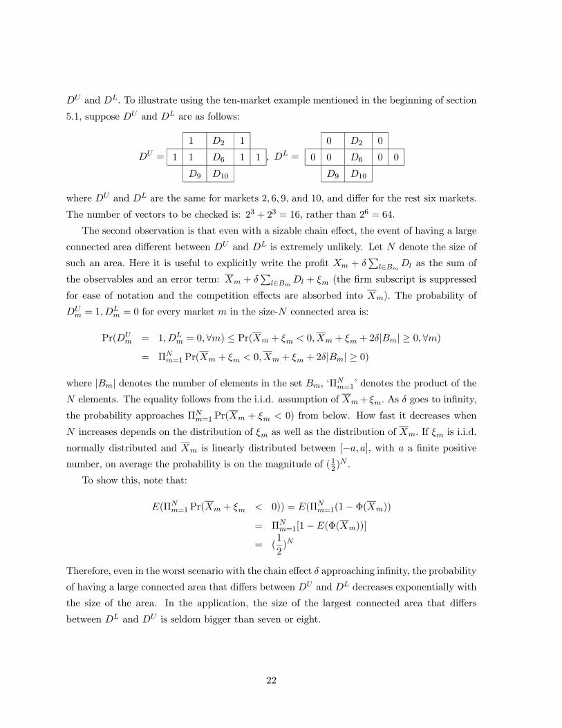
DU and DL. To illustrate using the ten-market example mentioned in the beginning of section

5.1, suppose DU and DL are as follows:

DU =

1 D2 1

1 1 D6 1 1

D9 D10

, DL =

0 D2 0

0 0 D6 0 0

D9 D10

where DU and DL are the same for markets 2, 6, 9, and 10, and differ for the rest six markets.

The number of vectors to be checked is: 23 + 23 = 16, rather than 26 = 64.

The second observation is that even with a sizable chain effect, the event of having a large

connected area different between DU and DL is extremely unlikely. Let N denote the size of

such an area. Here it is useful to explicitly write the profit Xm + δP

l∈BmDl as the sum of

the observables and an error term: Xm + δP

l∈BmDl + ξm (the firm subscript is suppressed

for ease of notation and the competition effects are absorbed into Xm). The probability of

DUm = 1,D

Lm = 0 for every market m in the size-N connected area is:

Pr(DUm = 1,DL

m = 0,∀m) ≤ Pr(Xm + ξm < 0,Xm + ξm + 2δ|Bm| ≥ 0,∀m)

= ΠNm=1 Pr(Xm + ξm < 0,Xm + ξm + 2δ|Bm| ≥ 0)

where |Bm| denotes the number of elements in the set Bm, ‘ΠNm=1’ denotes the product of the

N elements. The equality follows from the i.i.d. assumption of Xm+ ξm. As δ goes to infinity,

the probability approaches ΠNm=1 Pr(Xm + ξm < 0) from below. How fast it decreases when

N increases depends on the distribution of ξm as well as the distribution of Xm. If ξm is i.i.d.

normally distributed and Xm is linearly distributed between [−a, a], with a a finite positive

number, on average the probability is on the magnitude of (12)N .

To show this, note that:

E(ΠNm=1 Pr(Xm + ξm < 0)) = E(ΠNm=1(1− Φ(Xm))

= ΠNm=1[1−E(Φ(Xm))]

= (1

2)N

Therefore, even in the worst scenario with the chain effect δ approaching infinity, the probability

of having a large connected area that differs between DU and DL decreases exponentially with

the size of the area. In the application, the size of the largest connected area that differs

between DL and DU is seldom bigger than seven or eight.

22

5.5 Empirical implementation

The model does not yield a closed form solution to firms’ entry decisions and location

choices conditioning on market size observables and a given vector of parameter values. Thus

I adopt the simulation method. The most frequently used simulation methods for nonlinear

models are the method of simulated log-likelihood (MSL) and the method of simulated moments

(MSM). Implementing MSL is difficult because of the complexities in obtaining an estimate of

the log-likelihood of the observed sample. The cross-sectional dependence among the observed

outcomes in different markets indicates that the log-likelihood of the sample is no longer the

sum of the log-likelihood for each market, and one needs an exceptionally large number of

simulations to get a reasonable estimate of the sample’s likelihood. For this reason I use the

method of moments approach.

To estimate the parameters in the profit functions θ0 = βi, δii, δij , ρi=k,w,s ∈ Θ ⊂ RP , I

assume the following moment condition holds:

E[g(Xm, θ0)] = 0

where g(Xm, θ0) ∈ RL with L ≥ P is a vector of moment functions that specify the differences

between the observed equilibrium market structures and the those predicted by the model.

For example, one element of the vector function g(Xm, θ0) can be the difference between the

observed and the model predicted number of small retailers in market m.

A generalized method of moment (GMM) estimator, θ, minimizes a weighted quadratic

form in ΣMm=1g(Xm, θ) :

minθ∈Θ

1

M

∙MP

m=1g(Xm, θ)

¸0Ω

∙MP

m=1g(Xm, θ)

¸(4)

where Ω is an L × L positive semidefinite weighting matrix. Assume Ωp→ Ω0, an L × L

positive definite matrix. Define the L× P matrix G0 = E[∇θg(Xm, θ0)]. Under the standard

assumptions, including the g (Xm, θ) being i.i.d. across m, we have:

√M(θ − θ0)

d→ Normal(0,A−10 B0A−10 ) (5)

whereA0 ≡ G00Ω0G0, B0 =G

00Ω0Λ0Ω0G0, and Λ0 = E[g(Xm, θ0)g(Xm, θ0)

0] =Var[g(Xm, θ0)].

If a consistent estimator of Λ−10 is used as the weight matrix, then the GMM estimator θ is

asymptotically efficient, with its asymptotic variance being Avar(θ) = (G00Λ−10 G0)

−1/M.

The first obstacle in using this standard GMM method is that the chain effect in the profit

function induces cross sectional dependence of the equilibrium outcomes. The GMM estimator

remains consistent with such dependent data, but the covariance matrix needs to be corrected

23

to take the dependence into consideration. In particular, the asymptotic covariance matrix of

the moment functions in equation (5) should be replaced by Λd0 = Σs∈ME[g(X1, θ0)g(Xs, θ0)0].

Conley (1999) proposes a nonparametric covariance matrix estimator formed by taking a

weighted average of spatial autocovariance terms, with zero weights for observations farther

than a certain distance. The method requires some strong assumptions on the underlying

data generating process, including the mixing assumption that requires the dependence among

observations to die away quickly as the distance increases. In the current application the obser-

vations are in some sense spatially markovian, similar to the k-markovian random fields defined

in Huang and Cressie (2000), which implies strong mixing properties with rapidly declining

dependence as the ‘distance’ increases. In fact, there is only very weak dependence between

markets that do not directly border each other.

The covariance matrix estimator is analogous to the class of time-series spectral density

estimators whose time domain weights equal zero after a cutoff lag. Specifically, the estimator

of Λd0 that is used here is:

Λ ≡ 1

MΣmΣs∈Bm

£g(Xm, θ)g(Xm, θ)

0¤ (6)

where Bm is the set of direct neighbors of market m. That is, I average the spatial covariance

terms over bordering neighbors and apply zero weights to observations further away. The

variance estimates are similar if the summation is extended to the set of first nonbordering

neighbors.

The second obstacle in using the standard GMM is that g(Xm, θ) is difficult to obtain for

any given θ. For example, there is no closed form solution to the expected number of Wal-

Mart stores for a given market m. I adopt the simulation method developed by Pakes and

Pollard (1989) and McFadden (1989), where the difficult-to-calculate moment functions are

replaced with simulated unbiased estimates. The limit distribution of the simulated method

of moment estimator differs from GMM only through the presence of a scalar (1 +R−1) that

multiplies the variance matrix, which reflects the extra independent source of randomness

generated by the simulation process. The approach is as follows: start from some initial

guess of the parameter values, randomly draw from the normal distribution four independent

vectors: a vector of market common error εmMm=1 and three vectors of firm-specific errorsηk,mMm=1, ηw,mMm=1, and ηs,mMm=1. Obtain the simulated profits Πi, i = k,w, s and solve

for Dk, Dw, Ns. Repeat the simulation R times and formulate g(Xm, θ), an unbiased estimator

of g(Xm, θ). Evaluate the objective function (4) using g(Xm, θ) and search for the parameter

values that minimize the objective function, while using the same set of simulation draws for

all values of θ. To implement the two-step efficient estimator, I first use the identity matrix

24

as the weight Ω to find a consistent estimate θ, which is then plugged in (6) to compute the

optimal weight matrix Λ−1 for the second step.

Instead of the usual machine generated pseudo-random draws, I use Halton draws, which

have better coverage properties and smaller simulation variances.18 According to Train (2000),

100 Halton draws achieved greater accuracy in mixed logit estimation than 1000 pseudo-random

draws. I generate 150 Halton simulation draws for both the first stage and the second stage

estimation. The variance is calculated with 300 Halton draws.

There are twenty-six parameters with the following set of moments: the observed number

of Kmart stores, Wal-Mart stores, and small stores; the interaction between the market size

variables and the observed store number for each firm; the interaction of the various kinds of

market structures with the market size variables (for example, one market structure is that

there are Wal-Mart stores but no Kmart stores).

6 Results

6.1 Parameter Estimates

As mentioned in the data section, the sample includes 2065 small and medium sized

counties with populations between five thousand and sixty-four thousand. I take Kmart and

Wal-Mart’s store distribution in other counties as given, and only model their entry decisions

and their impact on small stores in the sample counties.

The profit functions of all retailers share three common explanatory variables: log of popu-

lation, log of real retail sales per capita, and the percentage of urban population. Many studies

have found that there is a pure size effect: there tends to be more stores in a market as the

population increases. Retail sales per capita capture the ‘depth’ of the market and seem to

explain the firm entry behavior better than personal income. The percentage of urban popu-

lation measures the degree of urbanization. It is generally believed that urbanized areas have

more shopping districts that attract big chain stores.

For Kmart, a dummy variable indicating whether the market is in the northern regions

is included in the profit function. Kmart’s headquarters are located in Troy, Michigan, and

until the mid 1980s this region has always been the ‘backyard’ of Kmart stores. Similarly,

Wal-Mart’s profit function includes a dummy variable for the southern regions, as well as the

log of distance (in miles) to its headquarters in Benton, Arkansas. Distance turns out to be

18The book by Kenneth Train ‘Discrete choice methods with simulation’ (2003) provides an excellent discussion

about Halton draws.

25

a useful predictor for Wal-Mart stores’ location choices. As for small stores, everything else

equal, there are more small stores in the southern states. It could be that there have always

been fewer big retail stores in the southern regions and people rely on neighborhood small

stores for day-to-day shopping.

All of the market size coefficients βi and the competitive effects δij are allowed to be firm

specific. Table 3 lists the parameter estimates for the years 1988 and 1997. The coefficients

for market size variables are highly significant and intuitive, with the exception of the urban

variable in the small stores’ profit function that suggests fewer small stores in more urbanized

areas. The competitive effects are also highly significant, except for the effect of small stores

on Kmart and Wal-Mart’s profits in 1997, which are not precisely estimated. ρ is much smaller

than 1, indicating the importance of controlling for the endogeneity of all firms’ entry decisions.

As mentioned in the previous sections, I estimate the model three times, each time using a

different equilibrium. Tables 4 (A) and 4 (B) present all of the three sets of estimates for years

1988 and 1997, respectively. Column one corresponds to the equilibrium most preferred by

Kmart; column two uses the equilibrium most preferred by Wal-Mart; column three chooses

the one that grants Wal-Mart an advantage in the southern regions and Kmart an advantage

in the rest of the country. The estimates are very robust across the different equilibria.

Table 5 displays the model’s goodness of fit. Columns one and three are the sample average

for the years 1988 and 1997, respectively; the other two columns are the model predicted

average. The model fits very well the sample mean of the number of counties with large

chains. For example, in 1988, 21% of the sample markets have Kmart and 32% have Wal-

Mart; the model’s predictions are 22% and 32%, respectively. For 1997, 19% of the sample

markets have Kmart and 48% have Wal-Mart; the model fits the sample means almost exactly.

For small stores, the sample average is 3.86 per county in 1988 and 3.49 per county in 1997;

the model’s predictions are 3.77 and 3.45. The number of small stores is a very noisy variable

and is much harder to predict. Its sample median is 3, but the maximum is 25 in 1987 and 19

in 1997. Overall, the model fits the data well.

To get an idea of how reasonable the estimates are, Table 6 lists the model’s predicted

profits and compares them with the accounting profits reported by Kmart and Wal-Mart in

their SEC 10-K annual reports. The model predicts that average profit for Wal-Mart stores

has increased 43% over the sample period, which matches very well the recorded increase of

38% in Wal-Mart’s annual reports from 1988 to 1997. Kmart’s accounting profit in 1997 is

substantially smaller than that in 1988, due to the financial obligations of divesting the various

specialized retailing businesses that were overall a financial disappointment. The average real

sales per Kmart store have increased only 2.6% over the ten-year period. Considering the

26

various increases in the operating costs mentioned in its annual report, the change in its sales

revenue is comparable with the 5% decrease in the store profit predicted by the model.19

To compare the magnitude of each coefficient, Table 7 reports the changes in the number of

stores when the market size variables change. For example, to derive the effect of population

change on the number of small stores, I fix Kmart and Wal-Mart’s profits and only increase

small retailers’ profit in accordance with a ten percent increase in the population. I re-solve

the model and calculate the average number of small stores for the sample.

The market size variables have a relatively modest impact on the number of small busi-

nesses. In 1988, a 10% increase in population attracts 9% more stores. The same increase in

real retail sales per capita draws five percent more stores. In comparison, the regional dummy

seems much more important: a market in the northern region has a third fewer small stores

than a market in the south with everything else equal. Market size variables seem to matter

more for big chains. A 10% increase in the population of every market induces Kmart and Wal-

Mart to enter 11% more markets. A similar increment in retail sales attracts entry of Kmart

and Wal-Mart stores in 16% and 12% additional markets, respectively. For both chains, the

regional advantage is substantial, although its importance is smaller in 1997.

6.2 The competition effect and the chain effect

The competition effect estimates in 1997 are very different from those in 1988. In par-

ticular, the negative effect of Kmart on Wal-Mart’s profit δwk has become much smaller (in

absolute value), while the opposite is true for Wal-Mart’s effect on Kmart’s profit δkw. Both

a Cournot model and a Bertrand model with differentiated products predict that reduction

in rivals’ marginal costs drives down a firm’s own profit. Since I do not observe firms’ mar-

ginal costs, I cannot directly incorporate them into the model. However, these parameter

estimates are consistent with anecdotal evidence suggesting that Wal-Mart’s marginal cost has

been declining relative to that of Kmart over the sample period. Wal-Mart is famous for its

cost-sensitive culture; it is also keen on technology advancement. For example, Holmes (2001)

cites evidence that Wal-Mart is a leading investor in information technologies. A CNBC doc-

19Wal-Mart’s 1988 and 1997 annual reports do not separate the profit of Wal-Mart stores from the profit of

Sam’s clubs. Since the gross markup in Sam’s clubs is half of that in the regular Wal-Mart discount stores, each

dollar sale from a Sam’s club is assumed to contribute to the total profit half as much as a dollar sale from a

Wal-Mart discount store. Supercenters, a combination of discount and grocery stores, first appearing in 1992

for Kmart and1994 for Wal-Mart, are on average twice as big as a regular discount store. In calculating the

revenue sales and net income per discount store, I assume that a supercenter’s revenue sales and net income

are twice that of a regular discount store. In 1997, supercenters account for 19\% of total Wal-Mart stores and

4.6\% of all Kmart stores. There are no supercenters in my sample.

27

umentary (2004) reports that Wal-Mart’s sophisticated computing facilities are second only to

those in the Pentagon. In contrast, Kmart has been struggling with its management failures

that have resulted in stagnant revenue sales and either delayed or abandoned store renovation

plans throughout the 1990s.

What is surprising is that the negative impact of Kmart on small firms’ profit δsk is com-

parable to that of Wal-Mart δsw, given that Wal-Mart has generated far more controversies (or

at least more media reports) than Kmart. It is probably because Wal-Mart has more stores in

the small to medium-sized markets and has kept expanding while Kmart is consolidating its

existing stores with few net openings in these markets.

It is somewhat difficult to understand why small firms have a negligible impact on big

firms’ profits (δks and δws) in 1997, while their impact is much more noticeable in 1988.

One explanation points to the relative change in the productivity of these stores, as Foster,

Haltiwanger and Krizan (2002) find that a large amount of the productivity growth in the

retail sector in the last decade is explained by the entry of more productive establishments

within a firm (chain).

Table 8 re-solves the model for different market structures. The results suggest that the

competition impact of chains on small stores is substantial. In 1988, compared with the

scenario where there are neither Kmart nor Wal-Mart stores, adding a Kmart store to each

market reduces the number of small stores by 48.7%, or 2.8 stores per county; adding a Wal-

Mart, 40.2%, or 2.3 stores per county; adding both a Kmart and a Wal-Mart store, 71.3%, or

4 stores per county. Interestingly, if Wal-Mart takes over Kmart, the number of small stores

is 9011, or 4.36 per county, 16% higher than that observed in the sample when Wal-Mart and

Kmart compete against each other. This is due to the existence of a business stealing effect:

the total number of chain stores is smaller after the take-over, which in turn leads to a larger

number of small stores. The patterns are quite similar in 1997: compared with the case of

no chain stores, adding a Kmart store to each market drives down the number of small stores

by 35.6%, or 1.9 stores per county; adding a Wal-Mart, 37.1%, or 2 stores per county; adding

both a Kmart and a Wal-Mart store, 61.5%, or 3.3 stores per county.

Even with the conservative estimate that one Kmart or Wal-Mart store replaces two small

stores, the competition effect of chains on small retailers is sizable, especially since the small

discount stores are only a segment of stores that are affected by the entry of chain stores. The

combined effect on all small retailers and the local community in general can be much larger.

The second panel of Table 8 illustrates the competition effect and the chain effect for Kmart

and Wal-Mart. Confirming the discussion above regarding the changes in δkw and δwk from

1988 to 1997, the effect of Kmart’s presence on Wal-Mart’s profit is much stronger in 1988,

28

while the effect of Wal-Mart’s presence on Kmart’s profit is stronger in 1997. For example, in

1988, Wal-Mart would only enter 318 markets if there is a Kmart store in every county. When

Kmart ceases to exist as a competitor, the number of markets with Wal-Mart stores rises to

847, a net increase of 166%. The same experiment in 1997 leads to 48.4% more entry, from

725 to 1080 markets. The pattern is reversed for Kmart. In 1988, Kmart would enter 23%

more markets when there is no Wal-Mart compared with the case of one Wal-Mart store in

every county; in 1997, Kmart would enter 96% more markets for the same experiment.20

In 1988, in the absence of the chain effect δww, Wal-Mart would enter 21.2% fewer markets,

from 655 to 516 markets. The difference reduces to only 6% in 1997. The change probably

reflects a smaller marginal benefit brought by an additional store as the chain gets bigger and

the scale economies are getting exhausted. For example, the savings in the distribution cost

per store when adding a store can be as high as fifty percent if there is only one store in the

region, while it is only two percent when there are already six stores in the region.

Overall, the chain effect does not seem to be an important consideration for Kmart. Tradi-

tionally, Kmart has relied on private vendors to deliver products to its stores, so the distribution

system is not an integrated part of the firm’s business. Also Kmart has focused on metropolitan

areas and avoided smaller counties, for fear of insufficient demand to support a large discount

store. Since not many counties in my sample belong to metropolitan areas, it is not surpris-

ing that I find little evidence of Kmart exploiting the potential scale economies arising from

locating stores close to each other. A study that also incorporates Kmart’s location choices in

larger counties would provide more convincing evidence of whether or not the chain effect is

important to Kmart.

As mentioned in section (4.3), the profit shocks are assumed to be cross-sectionally inde-

pendent, and the chain effect captures the net benefit of clustering stores in nearby markets.

One criticism is that the positive estimate is caused by the dependence among unobserved

demand shifters in nearby markets, rather than a consequence of scale economies. The data I

have do not allow me to separate these two explanations. However, if it is a demand-side story,

the same effect should appear in both Kmart and Wal-Mart’s profit functions. The small and

insignificant estimate in Kmart’s profit function, together with a large and significant estimate

in Wal-Mart’s profit function, suggests that this effect is firm specific, rather than demand-

driven. Also, Wal-Mart’s chain effect has declined substantially over the period and is not

precisely estimated in 1997. If the positive estimate is driven by demand factors, then one is

left to wonder why demand is cross-sectionally dependent in the late 1980s, but not so in the

20 In solving the number of Wal-Mart (Kmart) stores when Kmart (Wal-Mart) exits, I allow the small stores

to compete with the remaining chain.

29

late 1990s.

Another complication, which I have not discussed so far, is the cannibalization among

stores. Due to the localized nature of the retail demand, stores in different counties are not

likely to compete against each other, except when they are located near the county boundaries

of the counties and are geographically close to each other. To the extent that this effect exists,

the estimate of the chain effect is the net of the scale economies and the demand cannibalization.

It is therefore a lower bound to the true effect.21

6.3 The impact of Wal-Mart’s expansion and related policy issues

Consistent with the media reports on the impact of Wal-Mart stores on small retailers, the

model predicts that Wal-Mart’s expansion contributes to a large percentage of the net decline

in the number of small stores over the sample period.22 The first row in Table 9 displays

a net decrease of 748 small stores over the sample period, or 0.36 per market. To evaluate

the impact of Wal-Mart’s expansion on small stores separately from other factors (e.g., the

change in the market size or the change in Kmart stores), I re-solve the model using the 1988

coefficients for Kmart and small stores, the 1988 market size variables, but Wal-Mart’s 1997

coefficients. The experiment corresponds to the scenario where everything is kept the same

as in 1988, except that Wal-Mart is allowed to become more efficient and expand. Under this

scenario, the predicted number of small stores reduces from the baseline of 7777 to 7231.23

This is a net decrease of 546 stores, or 73% of what we observe in the data. To derive the

impact of market size changes on top of Wal-Mart’s expansion, I repeat the same exercise

but using the 1997 market size variables. The number of small stores increases by about 125

stores, or 17%, because both population and the real retail sales per capita have grown over the

sample period. Finally, using the 1997 profit coefficients for all firms and the 1997 market size

variables, the number of small stores decreases by another 240 stores, or 32%, to 7116 stores.

Altogether the model explains about 88% of the net change in the number of small stores and

leaves the remaining 12% (or about 87 stores) unexplained. Conducting the same experiment

but starting from the 1997 coefficients for Kmart and small stores, the results indicate that

21As discussed in section (4.1), the scale economies that affect all stores evenly, for example, the discount

associated with volume purchasing, cannot be separately identified from the constant in the profit function.

Therefore, there can be many other benefits enjoyed by a chain that are not captured by this model.22The number of markets with Kmart stores has declined slightly over the sample period, from 433 to 393

markets.23 In this simulation exercise, the equilibrium number of markets with a Wal-Mart store is 896, rather than

982 as observed in the data in 1997. The difference is explained by the changes in the market sizes between 1988

and 1997.

30

Wal-Mart’s expansion accounts for about 391 stores, or 52% of the decrease in the number of

small stores, with the remaining 36% is explained by the changes within the small retailers.

If we ignore the endogeneity of chains’ entry decisions and regress the number of small stores

on the number of chains together with the market size variables, we would underestimate the

impact of Wal-Mart’s expansion on small retailers by a large amount. For example, using the

1988 coefficients from an ordered probit model, the difference between the expected number

of small stores using Wal-Mart’s 1988 store number and the expected number of small stores

using Wal-Mart’s 1997 store number explains only 33% of the observed decline in the number

of small stores. Overall, ignoring the endogeneity underestimates the negative impact by fifty

to sixty percent.

Using the conservative figure of 391 stores, the absolute effect of Wal-Mart’s entry might

seem modest. However, the exercise here only include small stores in the discount sector. Since

both Kmart and Wal-Mart carry a large assortment of products and compete with a variety

of stores, like hardware stores, houseware stores, apparel stores, etc., their impact on the local

community is conceivably much larger. I am now in the process of estimating a model that

includes small stores in all of the major retail sectors that compete with these discount chains.

Results will be incorporated here once they are ready.

To examine the changes within small stores separately from the impact of chain stores, I

calculate small stores’ entry thresholds, the smallest population sizes that can accommodate

one small store, two small stores, etc., in the spirit of Bresnahan and Reiss (1991). Table 10

reports the entry thresholds in terms of thousands of population evaluated at the average retail

sales per capita and the average percentage of urban population for a county without chains.

The left three columns refer to the northern regions, while the right three columns refer to the

southern regions. From 1988 to 1997, the entry thresholds have increased across the board by

about 17-18% for the northern regions and 13-15% for the southern regions. For example, in

the northern regions, the minimum size to support three stores is 13,200 people in 1988, but

has increased to 15,470 people in 1997. Interestingly, similar to what Bresnahan and Reiss

(1991) have found, the entry threshold stabilizes after three stores, with about 6,000-7,000

population to support an additional store.

Without detailed information on small stores, it is difficult to understand why the entry

thresholds have increased between 1988 and 1997. One possible explanation is that the fixed

cost of establishing a store has increased. For instance, the barcode technology and the re-

lated electronic data exchange system might have become a necessity to compete in the retail

industry. Or it could be that the threat of entry by large chains exerts downward pressure on

prices, which has in turn lead to a reduced margin. Basker (2005), for example, finds evidence

31

that entry by Wal-Mart affects the city-level prices of various consumer products by 1.5-3% in

the short run, with an even larger impact in the long run.

Government subsidy has long been a policy instrument to encourage firm investment and to

create jobs. To evaluate the effectiveness of this policy in the discount retail sector, I simulate

the equilibrium number of stores when various firms are subsidized, which are summarized

in Table 11. The results indicate that a direct subsidy does not seem to be cost effective in

generating jobs. For example, subsidizing Wal-Mart stores 10% of its profit, which amounts

to one million dollars on average, only increases the number of Wal-Mart stores per county

from 0.317 to 0.342.24 With the average Wal-Mart store hiring less than 300 full and part-time

employees, the additional number of firms translates to at most eight new jobs.25 Similarly,

subsidizing all small stores by 100% of their profits increases the average number of small stores

by 0.83, or generates eight jobs if on average a small store hires ten employees. Together, these

exercises suggest that a direct subsidy should be used with caution if it is designed to increase

employment in this industry.

In 2004 Good Jobs First, a DC based research group, posted online a study documenting

that Wal-Mart has received a total of more than $1 billion US dollars from the state and

local governments in various forms of the economic development subsidies for 240 of its stores

and distribution centers. Most of these subsidies were granted in 1990s and 2000s. Table 12

reports the average profits for these subsidized stores (using the 1997 coefficient estimates)

and compares them with the profits for the rest of Wal-Mart stores. The first two rows list

the store profits for the sample counties; the last two rows list profits for counties bigger than

sixty-four thousand. Profits in larger counties are considerably higher. Interestingly, in both

cases the subsidized stores achieve a higher profit than the unsubsidized ones. For the sample

counties, the confidence intervals for the profits of the subsidized stores and the unsubsidized

ones do not overlap, suggesting the difference is significant at the 5% confidence level. The

pattern remains the same for the group of Wal-Mart stores in larger counties, although the

difference is not statistically significant.

Due to the poor disclosure quality of the economic development subsidies in most states,

the list of Wal-Mart stores that have received subsidies is far from complete; also there is no

publicly available information regarding the subsides Kmart and small stores have received.

24The average Wal-Mart store’s net income in 1988 is about one million in 2004 dollars (see Table 6). Using

a discount rate of 10%, the discounted present value of a store’s lifetime profit is about ten million. A subsidy

of 10% is equivalent to one million dollars.25The equilibrium numbers of Kmart stores and small stores decrease slightly when Wal-Mart is subsidized,

but the implied change in the number of employment is smaller than one.

32

It is therefore not possible to fully incorporate the subsidies into the model, and the results

above should be interpreted with this in mind. However, to the extent that many of these

development subsidies are granted for the purpose of attracting businesses to unprofitable

areas, the higher profits reported by subsidized Wal-Mart stores seem to suggest that entry

would have occurred even without these subsidies.

7 Conclusion and future work

This paper uses a structural model to examine the competition effect of chain stores on

small stores and the role of the chain effect in firms’ entry decisions and location choices. The

paper’s results support the anecdotal evidence that ‘big drives out small’. In particular, entry

by either Kmart or Wal-Mart displaces on average two small stores. Wal-Mart’s expansion

from the late 1980s to the late 1990s explains fifty to seventy percent of the net change in

the number of small discount stores. Failure to address the endogeneity of the firms’ entry

decisions results in underestimating this impact by fifty to sixty percent. Furthermore, direct

subsidies to either chain stores or small stores are not likely to be cost effective in creating jobs

and should be used with caution. The results in this paper reinforce the concerns raised by

many policy observers that subsidies to big retail corporations should be scrutinized. Perhaps

less obvious is the conclusion that subsidies toward small retailers should also be designed

carefully. The paper also finds that subsidized Wal-Mart stores are in general more profitable

than unsubsidized ones. Without more detailed information on these subsides, it is difficult

to assess whether these subsidies should be granted. However, it is probably safe to say that

entry would have occurred even without subsidization.

Like Holmes (2005), the paper finds that the scale economies, as captured by the chain

effect, generate substantial benefits. Future work that studies the particular nature of these

scale economies in more detail will be useful to understand how firms can better exploit them

and guide merger policies or other regulations that affect chains.

Finally, the algorithm proposed in this paper can be applied to other industries where scale

economies are important. One possible application is the airline industry, where the network of

flight routes exhibits a similar type of spillover effect as the one described here. For example,

adding a route from New York to Boston directly affects profits of flights that either originate

from or end in Boston and New York. The literature that studies this industry has ignored

this effect, due to the complicated nature of the related optimization problem. With the tools

proposed in this paper, one can extend current models of strategic interaction among airlines

to incorporate the network effects.

33

8 Appendix: Definitions and Proofs

1. Verification of the necessary condition in section (5.1)

Let the profit maximizer be denoted as D∗ = argmaxD∈DΠ(D). The optimality of D∗

implies a set of necessary conditions:

Π(D∗1, ...,D∗m−1,D

∗m,D

∗m+1, ...,D

∗M) ≥ Π(D∗1, ...,D∗m−1,Dm,D

∗m+1, ...,D

∗M),∀m,D∗m 6= Dm

Without loss of generality, let us assume market m has two neighbors: m− 1 and m+ 1.

Let D = D∗1, ...,D∗m−1,Dm,D∗m+1, ...,D

∗M. Π(D∗) differs from Π(D) at only three markets

m,m− 1, and m+1. At D, profits in markets m− 1 and m+1 are different from D∗ through

the chain effect. Let Bm−1\m denote the set of m − 1’s neighbors excluding market m.

Similarly, Bm+1\m denotes m+ 1’s neighbors except for market m. The difference between

Π(D∗) and Π(D) is:

Π(D∗)−Π(D) = D∗m−1(Xm−1 + δΣl∈Bm−1\mD∗l + δD∗m) +D∗m(Xm + δΣl∈BmD

∗l ) +

D∗m+1(Xm+1 + δΣl∈Bm+1\mD∗l + δD∗m)+

−D∗m−1(Xm−1 + δΣl∈Bm−1\mD∗l + δDm) +

Dm(Xm + δΣl∈BmD∗l ) +D∗m+1(Xm+1 + δΣl∈Bm+1\mD

∗l + δDm)

= (D∗m −Dm)£Xm + δΣl∈BmD

∗l + δ(D∗m−1 +D∗m−1)

¤= (D∗m −Dm) [Xm + 2δΣl∈BmD

∗l ]

The last equality follows from the assumption that market m has two neighbors: Bm = m−1,m + 1. Since Π(D∗) − Π(D) ≥ 0 for any value of D∗m and Dm, with D∗m 6= Dm, we have

D∗m = 1,Dm = 0 iff Xm + 2δΣl∈BmD∗l ≤ 0; and D∗m = 0,Dm = 1 iff Xm + 2δΣl∈BmD

∗l ≤ 0.

Together they imply D∗m = 1[Xm + 2δP

l∈BmD∗l ≥ 0], which is the necessary condition (3)

mentioned in section 5.1.

2. The set of fixed points of an increasing function that maps a lattice into itself

In the estimation, the definition of a lattice involves the notions of a partially ordered set,

a join, and a meet. A partially ordered set is a set D on which there is a binary relation ¹ thatis reflexive, antisymmetric, and transitive. If two elements, D0 and D00, of a partially ordered

set D have a least upper bound (greatest lower bound) in D, it is their join (meet) and is

denoted D0 ∨D00 (D0 ∧D00).

34

Definition 1 (Lattice) A partially ordered set that contains the join and the meet of each

pair of its elements is a lattice.

Definition 2 (Complete lattice) A lattice in which each nonempty subset has a supremum

and an infimum is complete.

Any finite lattice is complete. A nonempty complete lattice has a greatest element and a

least element. Corollary (2.5.1) says the set of fixed points of an increasing function from a

lattice onto itself is a nonempty complete lattice with a greatest element and a least element.

Corollary (2.5.1) Suppose that V (D) is an increasing function from a nonempty complete

lattice D into D.

(a) The set of fixed points of V (D) is nonempty, supD(D ∈ D,D ≤ V (D)) is the greatestfixed point, and infD(D ∈ D, V (D) ≤ D) is the least fixed point.

(b) The set of fixed points of V (D) in D is a nonempty complete lattice.

For a counter example where a decreasing function’s set of fixed points is empty, consider

the following simplified entry model where three firms compete with each other and decide

simultaneous whether to enter the market. Their joint choice set is D = 0, 13. The profitfunctions are as follows: ⎧⎪⎪⎨⎪⎪⎩

Πk = Dk(0.5−Dw − 0.25Ds)

Πw = Dw(1− 0.5Dk − 1.1Ds)

Πs = Ds(0.6− 0.5Dw − 0.7Ds)

LetD = Dk,Dw,Ds ∈ D, D−i denote rivals’ strategies, Vi(D−i) denote the best response

function for player i, and V (D) = Vk(D−k), Vw(D−w), Vs(D−s) denote the joint best responsefunction. It is easy to show that V (D) is a decreasing function that takes the following values:(

V (0, 0, 0) = 1, 1, 1; V (0, 0, 1) = 1, 0, 1; V (0, 1, 0) = 0, 1, 1; V (0, 1, 1) = 0, 0, 1V (1, 0, 0) = 1, 1, 0; V (1, 0, 1) = 1, 0, 0; V (1, 1, 0) = 0, 1, 0; V (1, 1, 1) = 0, 0, 0

The set of fixed points for V (D) is empty, since there does not exist a D ∈ D such that

V (D) = D.

3. A tighter lower bound and upper bound for the optimal solution vector D∗

In section 5.1 I have showed that using D = inf(D) and D = sup(D) as starting points, one

gets a lower bound and an upper bound to the argmax of the chain’s maximization problem:

maxD1,...,DM∈0,1

Π =MX

m=1

⎡⎣Dm ∗ (Xm + δXl∈Bm

Dl)

⎤⎦35

Here I introduce two bounds that are much tighter. The lower bound builds on the solution

to a constrained maximization problem:

maxD1,...,DM∈0,1

Π =MXi=1

⎡⎣Dm ∗ (Xm + δXl∈Bm

Dl)

⎤⎦s.t. if Dm = 1, then Xm + δ

Xl∈Bm

Dl > 0

Notice that the solution to this constrained maximization problem belongs to the set of

fixed points of the vector function V (D) = V1(D), ..., VM(D), where Vm(D) = 1[Xm +

δP

l∈BmDl ≥ 0]. Again V (·) is an increasing vector function that maps from D onto itself:

V : D→ D. Using similar arguments to those in section 5.1, one can show that the convergent

vector D using D0 = sup(D) as the starting vector is the greatest element of the set of fixed

points. Further this greatest element achieves a higher profit than any other fixed point, since

by construction each non-zero element of the vector D adds a positive component to the total

profit. Changing any non-zero element(s) of D to zero reduces the total profit.

To show that D is a lower bound toD∗, the solution to the original unconstrained maximiza-

tion problem, we construct a contradiction. Since the maximum profit of the unconstrained

problem is weakly higher than that of the constrained problem, i.e., Π(D∗) ≥ Π(D), D∗ can’tbe strictly smaller than D, because any vector strictly smaller than D delivers a lower profit.

Suppose D∗ and D are unordered. Let D∗∗ = D∗∨D (where ‘∨’ defines the element-by-elementMax operation). The change from D∗ to D∗∗ increases total profit. This is because profits at

markets with D∗m = 1 are not decreasing after the change, and profits at markets with D∗m = 0

but Dm = 1 increase from 0 to a positive number after the change. This contradicts to the

definition of D∗, so D ≤ D∗.

Using D as a starting point will produce a tighter lower bound than DL discussed in section

5.1. First note that V (D) ≥ D, where V (·) is as defined in section (5.1). This follows fromVm(D) = 1[Xm + 2δ

Pl∈Bm

Dl ≥ 0] ≥ 1[Xm + δP

l∈BmDl ≥ 0] = Dm,∀m, with the first and

the last equality being the definitions of Vm(·) and Dm, respectively. Again the monotonicity

of V (·) implies that iterating V on D converges in T steps with T ≤M. The convergent vector

DT is a lower bound to D∗ because D ≤ D∗ and DT = V T (D) ≤ V T (D∗) = D∗. DT is a much

tighter lower bound than DL because D ≥ D0 = inf(D), so DT = V TT (D) ≥ V TT (D0) = DL,

with TT = maxT, T 0 where T is the number of steps from D to DT and T 0 is the number of

steps from D0 to DL.

A tighter upper bound can also be found by using the vector D = Dm : Dm = 0 if

Xm+2δ|Bm| < 0; Dm = 1 otherwise. The markets with Dm = 0 always contribute a negative

36

element to the total profit and it is never optimal to enter these markets, i.e., D ≥ D∗. It is

straight forward to show that V (D) ≤ D. These two properties guarantee that the process

using D as a starting point converges and the convergent vector is an upper bound to D∗.

Together D and D are two starting points that produce a very tight lower bound and upper

bound to D∗, and are used in place of D = sup(D) and D = inf(D) in the estimation.

4. Verification of the profit function being supermodular with decreasing differences

Definition 3 (Supermodular (submodular) functions) Suppose that f(D) is a real-valued

function on a lattice D. If

f(D0) + f(D00) ≤ f(D0 ∨D00) + f(D0 ∧D00) (7)

for all D0 and D00 in D, then f(D) is supermodular on D. If

f(D0) + f(D00) < f(D0 ∨D00) + f(D0 ∧D00)

for all unordered D0 and D00 in D, then f(D) is strictly supermodular on D. If −f(D) is(strictly) supermodular, then f(D) is (strictly) submodular.

Definition 4 (Increasing (decreasing) differences) Suppose that D and T are partially

ordered sets and f(D, t) is a real-valued function on D×T. If f(D, t00)−f(D, t0) is increasing,

decreasing,strictly increasing, or strictly decreasing in D on D for all t0 ≺ t00 in T , then f(D, t)

has, respectively, increasing differences, decreasing differences, strictly increasing differences,

or strictly decreasing differences in (D, t) on D.

The following verifies that the profit function

Πi =MX

m=1

⎡⎣Di,m ∗ (Xm + δiiXl∈Bm

Di,l + δijDj,m)

⎤⎦=

MXm=1

⎡⎣Di,m ∗ (Xm + δiiXl∈Bm

Di,l)

⎤⎦is supermodular in its own strategy Di ∈ D. For ease of notation, the firm subscript i is

omitted. First it is easy to show that D0 ∨D00 = (D0 −min(D0,D00)) + (D00 −min(D0,D00)) +

min(D0,D00), D0∧D00 = min(D0,D00). LetD0−min(D0,D00) be denoted asD1, D00−min(D0,D00)

37

as D2, and min(D0,D00) as D3.The left-hand side of the condition (7) is:

Π(D0) +Π(D00) = ΣmD0m(Xm + δΣl∈BmD

0l) + ΣmD

00m(Xm + δΣl∈BmD

00l )

= Σm[(D0m −min(D0

m,D00m)) + min(D

0m,D

00m)](Xm +

δΣl∈Bm [(D0l −min(D0

l,D00l )) + min(D

0l,D

00l )])+

Σm[(D00m −min(D0

m,D00m)) + min(D

0m,D

00m)](Xm +

δΣl∈Bm [(D00l −min(D0

l,D00l )) + min(D

0l,D

00l )])

= Σm(D1,m +D3,m)(Xm + δΣl∈Bm(D1,l +D3,l)) +

Σm(D2,m +D3,m)(Xm + δΣl∈Bm(D2,l +D3,l))

Similarly, the right-hand side of the condition (7) is:

Π(D0 ∨D00) +Π(D0 ∧D00) = Σm(D0m ∨D00

m)(Xm + δΣl∈Bm(D0l ∨D00

l )) +

Σm(D0m ∧D00

m)(Xm + δΣl∈Bm(D0l ∧D00

l ))

= Σm(D1,m +D2,m +D3,m)(Xm + δΣl∈Bm(D1,l +D2,l +D3,l)) +

ΣmD3,m(Xm + δΣl∈BmD3,l)

= Π(D0) +Π(D00) + δ(ΣmD2,mΣl∈BmD1,l +ΣmD1,mΣl∈BmD2,l)

The profit function is supermodular in its own strategy if the chain effect δ is positive. The

verification for the decreasing differences is straight forward:

Πi(Di,D00j )−Πi(Di,D

0j) =

MXm=1

⎡⎣Di,m ∗ (Xm + δiiXl∈Bm

Di,l + δijD00j,m)

⎤⎦−MX

m=1

⎡⎣Di,m ∗ (Xm + δiiXl∈Bm

Di,l + δijD0j,m)

⎤⎦= δij

MXm=1

Di,m(D00j,m −D0

j,m)

The difference is decreasing in Di for all D0j < D00

j as long as δij < 0.

5. Multiple maximizers to the chain’s optimization problem

In the estimation section, I have assumed that the optimal solution to the chain’s problem is

unique. Before applying theorem (2.4.3) and theorem (2.8.1) to discuss the solution algorithm

when the set of argmax contains more than one element, I need to introduce the definition of

the induced set ordering. Here the notion of induced set ordering is defined on lattices.

38

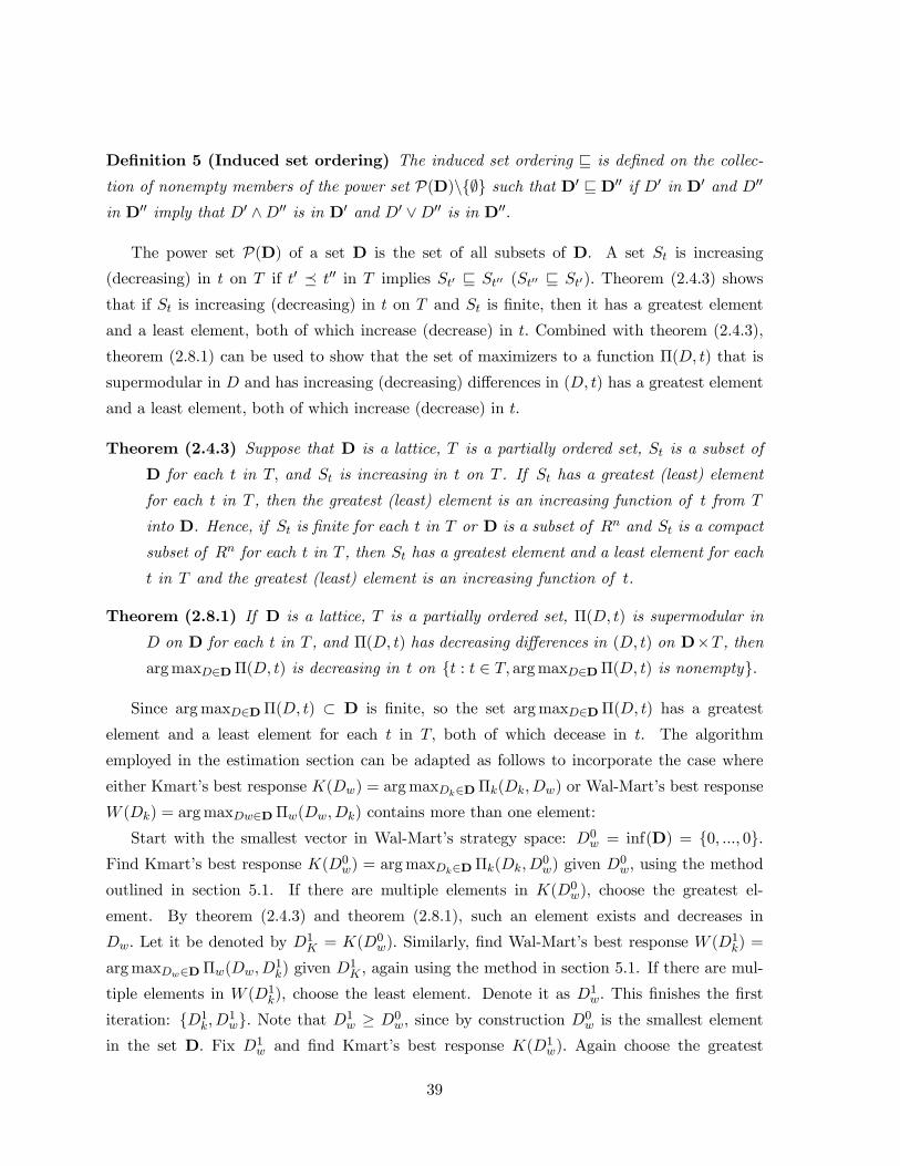
Definition 5 (Induced set ordering) The induced set ordering v is defined on the collec-

tion of nonempty members of the power set P(D)\∅ such that D0 v D00 if D0 in D0 and D00

in D00 imply that D0 ∧D00 is in D0 and D0 ∨D00 is in D00.

The power set P(D) of a set D is the set of all subsets of D. A set St is increasing

(decreasing) in t on T if t0 ¹ t00 in T implies St0 v St00 (St00 v St0). Theorem (2.4.3) shows

that if St is increasing (decreasing) in t on T and St is finite, then it has a greatest element

and a least element, both of which increase (decrease) in t. Combined with theorem (2.4.3),

theorem (2.8.1) can be used to show that the set of maximizers to a function Π(D, t) that is

supermodular in D and has increasing (decreasing) differences in (D, t) has a greatest element

and a least element, both of which increase (decrease) in t.

Theorem (2.4.3) Suppose that D is a lattice, T is a partially ordered set, St is a subset of

D for each t in T, and St is increasing in t on T . If St has a greatest (least) element

for each t in T , then the greatest (least) element is an increasing function of t from T

into D. Hence, if St is finite for each t in T or D is a subset of Rn and St is a compact

subset of Rn for each t in T , then St has a greatest element and a least element for each

t in T and the greatest (least) element is an increasing function of t.

Theorem (2.8.1) If D is a lattice, T is a partially ordered set, Π(D, t) is supermodular in

D on D for each t in T , and Π(D, t) has decreasing differences in (D, t) on D×T , then

argmaxD∈DΠ(D, t) is decreasing in t on t : t ∈ T, argmaxD∈DΠ(D, t) is nonempty.

Since argmaxD∈DΠ(D, t) ⊂ D is finite, so the set argmaxD∈DΠ(D, t) has a greatest

element and a least element for each t in T, both of which decease in t. The algorithm

employed in the estimation section can be adapted as follows to incorporate the case where

either Kmart’s best response K(Dw) = argmaxDk∈DΠk(Dk,Dw) or Wal-Mart’s best response

W (Dk) = argmaxDw∈DΠw(Dw,Dk) contains more than one element:

Start with the smallest vector in Wal-Mart’s strategy space: D0w = inf(D) = 0, ..., 0.

Find Kmart’s best response K(D0w) = argmaxDk∈DΠk(Dk,D

0w) given D0

w, using the method

outlined in section 5.1. If there are multiple elements in K(D0w), choose the greatest el-

ement. By theorem (2.4.3) and theorem (2.8.1), such an element exists and decreases in

Dw. Let it be denoted by D1K = K(D0

w). Similarly, find Wal-Mart’s best response W (D1k) =

argmaxDw∈DΠw(Dw,D1k) given D1

K , again using the method in section 5.1. If there are mul-

tiple elements in W (D1k), choose the least element. Denote it as D

1w. This finishes the first

iteration: D1k,D

1w. Note that D1

w ≥ D0w, since by construction D0

w is the smallest element

in the set D. Fix D1w and find Kmart’s best response K(D1

w). Again choose the greatest

39

element in K(D1w) and let it be denoted by D2

k = K(D1w). By theorem (2.4.3) and theo-

rem (2.8.1), D2k ≤ D1

k. The same argument shows that D2w ≥ D1

w. Iterate until convergence:

DTk = DT−1

k , and DTw = DT−1

w . Since both Dk and Dw can change their values no more than

M times, the algorithm converges in T steps with T ≤M. The convergent vector (DTk ,D

Tw) is

an equilibrium:DTk = K(DT

w), DTw = W (DT

k ). The same argument in section 5.2 shows that

this equilibrium generates the highest profit for Kmart among the set of all equilibria. The

case with the equilibrium that grants Wal-Mart the highest profit is similar.

40

References

[1] Andrews, Donald W.K., Steven Berry, and Panle Jia (2004), “Confidence Re-

gions for Parameters in Discrete Games with Multiple Equilibria”, Yale University working

paper.

[2] Bajari, Patrick, Han Hong, and Stephen Ryan (2004), “Identification and Estima-

tion of Discrete Games of Complete Information”, Duke University working paper.

[3] Basker, Emek (2005), “Selling a Cheaper Mousetrap: Wal-Mart’s Effect on Retail

Prices”, Journal of Urban Economics, Vol. 58, No. 2, pp. 203-229.

[4] Basker, Emek (2005), “Job Creation or Destruction? Labor-Market Effects of Wal-Mart

Expansion”, The Review of Economics and Statistics, vol. 87, No. 1, pp. 174-183.

[5] Berry, Steven (1992), “Estimation of a Model of Entry in the Airline Industry”, Econo-

metrica, vol 60, No. 4, pp. 889-917.

[6] Bresnahan, Timothy and Peter Reiss (1990), “Entry into Monopoly Markets”, Re-

view of Economic Studies, vol. 57, No. 4, pp. 531-553.

[7] Bresnahan, Timothy and Peter Reiss (1991), “Entry and Competition in Concen-

trated Markets”, Journal of Political Economy, vol. 95, No. 5, pp. 57-81.

[8] Chernozhukov, Victor, Han Hong, and Elie Tamer (2004), “Inference on Para-

meter Set in Econometric Models”, Princeton University working paper.

[9] Committee on Small Business. House (1994), “Impact of Discount Superstores on

Small Business and Local Communities”, Committee Serial No. 103-99. Congressional

Information Services, Inc.

[10] CNBC documentary (2004) “The Age of Wal-Mart: Inside America’s Most Powerful

Company”.

[11] Conley, Timothy (1999), “GMM Estimation with Cross Sectional Dependence”, Jour-

nal of Econometrics, Vol. 92, pp. 1-45.

[12] Davis, Peter (2005) “Spatial Competition in Retail Markets: Movie Theaters”, forth-

coming RAND Journal of Economics.

[13] Directory of Discount Department Stores (1988-1997), Chain Store Guide, Busi-

ness Guides, Inc., New York.

41

[14] Discount Merchandiser (1988-1997), Schwartz Publications, New York.

[15] Foster, Lucia, John Haltiwanger, and C.J. Krizan (2002), “The Link Between

Aggregate and Micro Productivity Growth: Evidence from Retail Trade”, NBER working

paper, No. 9120.

[16] Hajivassiliou, Vassilis (1997), “Some Practical Issues in Maximum Simulated Likeli-

hood”, in Roberto Mariano, Til Schuermann and Melvyn J. Weeks (eds.), Simulation-based

inference in econometrics (Cambridge University Press), 2000, pp. 71-99.

[17] Holmes, Thomas (2001), “Barcodes lead to Frequent Deliveries and Superstores”,

RAND Journal of Economics, Vol. 32, No. 4, pp. 708-725.

[18] Holmes, Thomas (2005), “The Diffusion of Wal-Mart and Economies of Density”, Uni-

versity of Minnesota working paper.

[19] Huang, Hsin-Cheng and Noel Cressie (2000), “Asymptotic Properties of Maxi-

mum (Composite) Likelihood Estimators for Partially Ordered Markov Models”, Statistica

Sinica, vol. 10, pp. 1325-1344.

[20] Kmart Inc. (1988-2000), Annual Report.

[21] Mazzeo, Michael (2002), “Product Choice and Oligopoly Market Structure”, RAND

Journal of Economics, vol. 33, No. 2, pp. 1-22.

[22] McFadden, Daniel (1989), “A Method of Simulated Moments for Estimation of Discrete

Response Models without Numerical Integration”, Econometrica, vol. 57, No. 5, pp. 995-

1026.

[23] Pakes, Ariel and David Pollard, “Simulation and the Asymptotics of Optimization

Estimators”, Econometrica, vol. 57, No. 5, pp. 1027-1057.

[24] Pakes, Ariel, Jack Porter, Kate Ho, and Joy Ishii (2005), “Moment Inequalities

and Their Application”, Harvard working paper.

[25] Pinkse, Joris, Margaret Slade, and Craig Brett (2002), “Spatial Price Compe-

tition: A Semiparametric Approach”, Econometrica, Vol. 70, No. 3, pp. 1111-1153.

[26] Seim, Katja (2005), “An Empirical Model of Firm Entry with Endogenous Product-Type

Choices”, forthcoming RAND Journal of Economics.

42

[27] Shils, Edward B. (1997), “Measuring the Economic and Sociological Impact of the

Mega-Retail Discount Chains on Small Enterprise in Urban, Suburban and Rural Com-

munities”, online: http://www.lawmall.com/rpa/rpashils.htm.

[28] Smith, Howard (2004), “Supermarket Choice and Supermarket Competition in Market

Equilibrium”, Review of Economic Studies, vol. 71, No. 1, pp. 235-263.

[29] Stone, Keneth (1995), “Impact of Wal-Mart Stores On Iowa Communities: 1983-93”,

Economic Development Review, Vol. 13, No. 2, pp. 60-69.

[30] Taylor, Don, and Jeanne Archer (1994), “Up Against the Wal-Marts (How Your

Business Can Survive in the Shadow of the Retail Giants)”, New York: American Man-

agement Association.

[31] Topkis, Donald (1979), “Equilibrium Points in Nonzero-Sum n-Person Submodular

Games”, SIAM Journal of Control and Optimum, Vol 17, pp 773-787.

[32] Topkis, Donald (1998), “Supermodularity and Complementarity”, Princeton University

Press, New Jersey.

[33] Train, Kenneth (2000), “Halton Sequences for Mixed Logit,” UC Berkeley working

paper.

[34] Vance, Sandra S., and Roy V. Scott (1994), “A History of Sam Walton’s Retail

Phenomenon”, Twayne Publishers, New York.

[35] Wal-Mart Stores, Inc. (1970-2000), Annual Report.

[36] Zhou, Lin (1994), “The Set of Nash Equilibria of a Supermodular Game Is a Complete

Lattice”, Games and Economic Behavior, Vol. 7, pp 295-300.

43

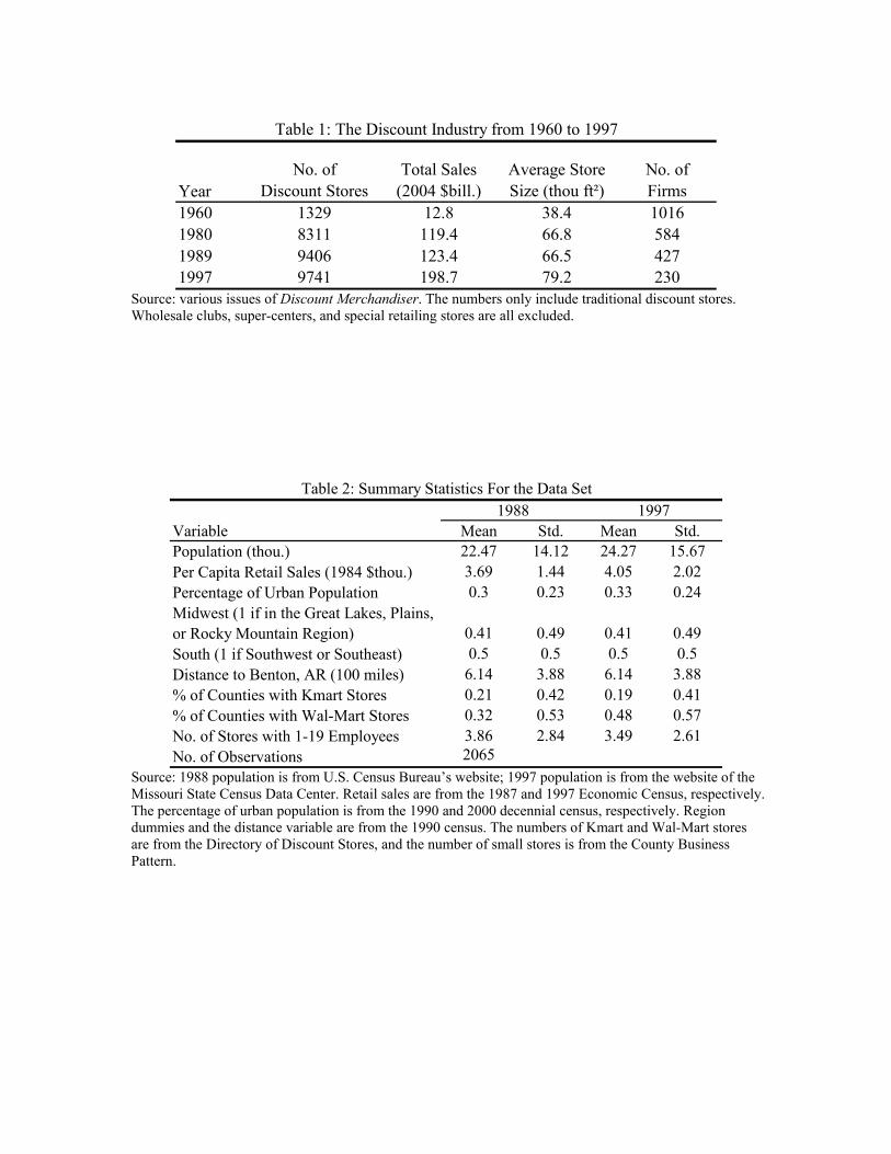
YearNo. of

Discount StoresTotal Sales

(2004 $bill.)Average StoreSize (thou ft²)

No. ofFirms

1960 1329 12.8 38.4 10161980 8311 119.4 66.8 5841989 9406 123.4 66.5 4271997 9741 198.7 79.2 230

Table 1: The Discount Industry from 1960 to 1997

Source: various issues of Discount Merchandiser. The numbers only include traditional discount stores. Wholesale clubs, super-centers, and special retailing stores are all excluded.

Variable Mean Std. Mean Std.Population (thou.) 22.47 14.12 24.27 15.67Per Capita Retail Sales (1984 $thou.) 3.69 1.44 4.05 2.02Percentage of Urban Population 0.3 0.23 0.33 0.24Midwest (1 if in the Great Lakes, Plains, or Rocky Mountain Region) 0.41 0.49 0.41 0.49South (1 if Southwest or Southeast) 0.5 0.5 0.5 0.5Distance to Benton, AR (100 miles) 6.14 3.88 6.14 3.88% of Counties with Kmart Stores 0.21 0.42 0.19 0.41% of Counties with Wal-Mart Stores 0.32 0.53 0.48 0.57No. of Stores with 1-19 Employees 3.86 2.84 3.49 2.61No. of Observations 2065

1988 1997Table 2: Summary Statistics For the Data Set

Source: 1988 population is from U.S. Census Bureau’s website; 1997 population is from the website of the Missouri State Census Data Center. Retail sales are from the 1987 and 1997 Economic Census, respectively. The percentage of urban population is from the 1990 and 2000 decennial census, respectively. Region dummies and the distance variable are from the 1990 census. The numbers of Kmart and Wal-Mart stores are from the Directory of Discount Stores, and the number of small stores is from the County Business Pattern.

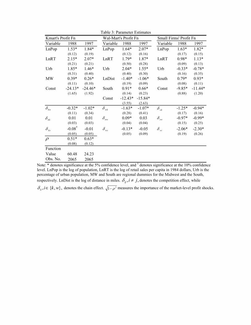
Kmart's Profit Fn Wal-Mart's Profit Fn Small Firms' Profit FnVariable 1988 1997 Variable 1988 1997 Variable 1988 1997LnPop 1.53* 1.84* LnPop 1.64* 2.07* LnPop 1.63* 1.82*

(0.12) (0.19) (0.12) (0.16) (0.17) (0.15)LnRT 2.15* 2.07* LnRT 1.79* 1.87* LnRT 0.98* 1.13*

(0.21) (0.21) (0.50) (0.28) (0.09) (0.13)Urb 1.85* 1.46* Urb 2.04* 1.55* Urb -0.33* -0.78*

(0.31) (0.40) (0.40) (0.30) (0.16) (0.35)MW 0.39* 0.26* LnDist -1.40* -1.06* South 0.79* 0.93*

(0.11) (0.10) (0.19) (0.09) (0.08) (0.11)Const -24.13* -24.46* South 0.91* 0.66* Const -9.85* -11.44*

(1.65) (1.92) (0.14) (0.23) (0.88) (1.20)Const -12.43* -15.84*

(3.55) (2.63)-0.32* -1.02* -1.63* -1.07* -1.25* -0.94*(0.11) (0.34) (0.28) (0.41) (0.17) (0.16)0.01 0.01 0.09* 0.03 -0.97* -0.99*(0.03) (0.03) (0.04) (0.04) (0.15) (0.25)

-0.08† -0.01 -0.13* -0.05 -2.06* -2.30*(0.05) (0.05) (0.05) (0.09) (0.19) (0.26)0.51* 0.63*(0.08) (0.12)

FunctionValue 60.48 24.23Obs. No. 2065 2065

Table 3: Parameter Estimates

kwδ

kkδ

ksδ

ρ

wkδ

wwδ

wsδ

skδ

swδ

ssδ

Note: * denotes significance at the 5% confidence level, and † denotes significance at the 10% confidence level. LnPop is the log of population, LnRT is the log of retail sales per capita in 1984 dollars, Urb is the percentage of urban population, MW and South are regional dummies for the Midwest and the South, respectively. LnDist is the log of distance in miles. , ,ij i jδ ≠ denotes the competition effect, while

, , ,ii i k wδ ∈ denotes the chain effect. 21 ρ− measures the importance of the market-level profit shocks.

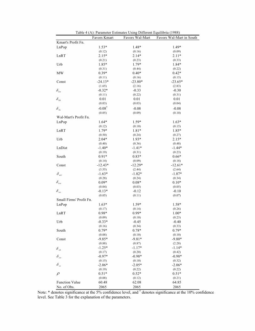
Favors Kmart Favors Wal-Mart Favors Wal-Mart in SouthKmart's Profit Fn.LnPop 1.53* 1.48* 1.49*

(0.12) (0.16) (0.09)LnRT 2.15* 2.14* 2.11*

(0.21) (0.23) (0.33)Urb 1.85* 1.79* 1.84*

(0.31) (0.44) (0.22)MW 0.39* 0.40* 0.42*

(0.11) (0.16) (0.15)Const -24.13* -23.80* -23.65*

(1.65) (2.16) (2.83)-0.32* -0.33 -0.30(0.11) (0.22) (0.31)0.01 0.01 0.01(0.03) (0.03) (0.04)

-0.08† -0.08 -0.08(0.05) (0.09) (0.10)

Wal-Mart's Profit Fn.LnPop 1.64* 1.59* 1.63*

(0.12) (0.10) (0.15)LnRT 1.79* 1.81* 1.85*

(0.50) (0.24) (0.27)Urb 2.04* 1.93* 2.15*

(0.40) (0.36) (0.48)LnDist -1.40* -1.41* -1.44*

(0.19) (0.31) (0.23)South 0.91* 0.83* 0.66*

(0.14) (0.09) (0.18)Const -12.43* -12.29* -12.61*

(3.55) (2.44) (2.64)-1.63* -1.82* -1.87*(0.28) (0.24) (0.34)0.09* 0.08* 0.10*(0.04) (0.03) (0.05)

-0.13* -0.12 -0.10(0.05) (0.11) (0.07)

Small Firms' Profit Fn.LnPop 1.63* 1.59* 1.58*

(0.17) (0.14) (0.26)LnRT 0.98* 0.99* 1.00*

(0.09) (0.10) (0.23)Urb -0.33* -0.45 -0.40

(0.16) (0.34) (0.33)South 0.79* 0.78* 0.79*

(0.08) (0.10) (0.10)Const -9.85* -9.81* -9.80*

(0.88) (0.87) (2.28)-1.25* -1.17* -1.14*(0.17) (0.20) (0.42)

-0.97* -0.98* -0.98*(0.15) (0.10) (0.32)

-2.06* -2.05* -2.06*(0.19) (0.22) (0.22)0.51* 0.52* 0.51*(0.08) (0.12) (0.21)

Function Value 60.48 62.08 64.85No. of Obs. 2065 2065 2065

Table 4 (A): Parameter Estimates Using Different Equilibria (1988)

ρ

wwδ

wsδ

skδ

swδ

kkδ

ksδ

wkδ

ssδ

kwδ

Note: * denotes significance at the 5% confidence level, and † denotes significance at the 10% confidence level. See Table 3 for the explanation of the parameters.

Favors Kmart Favors Wal-Mart Favors Wal-Mart in SouthKmart's Profit Fn.LnPop 1.84* 1.78* 1.79*

(0.19) (0.18) (0.12)LnRT 2.07* 1.98* 1.99*

(0.21) (0.28) (0.26)Urb 1.46* 1.37* 1.40*

(0.40) (0.34) (0.31)MW 0.26* 0.29 0.13†

(0.10) (0.22) (0.07)Const -24.46* -23.11* -23.47*

(1.92) (2.36) (2.19)-1.02* -1.12* -1.00*(0.34) (0.24) (0.27)0.01 0.01 0.04(0.03) (0.08) (0.05)-0.01 -0.04 -0.04(0.05) (0.06) (0.11)

Wal-Mart's Profit Fn.LnPop 2.07* 1.98* 2.05*

(0.16) (0.12) (0.15)LnRT 1.87* 1.75* 1.81*

(0.28) (0.24) (0.12)Urb 1.55* 1.44* 1.53*

(0.30) (0.36) (0.55)LnDist -1.06* -1.08* -1.02*

(0.09) (0.10) (0.09)South 0.66* 0.71* 0.51*

(0.23) (0.19) (0.12)Const -15.84* -14.44* -15.39*

(2.63) (1.99) (1.22)-1.07* -1.23* -1.05*(0.41) (0.21) (0.22)0.03 0.03 0.03(0.04) (0.02) (0.03)-0.05 -0.11 -0.05(0.09) (0.11) (0.09)

Small Firms' Profit Fn.LnPop 1.82* 1.75* 1.70*

(0.15) (0.17) (0.14)LnRT 1.13* 1.08* 1.03*

(0.13) (0.12) (0.09)Urb -0.78* -0.79* -0.50†

(0.35) (0.28) (0.26)South 0.93* 0.90* 0.90*

(0.11) (0.11) (0.10)Const -11.44* -11.02* -10.49*

(1.20) (1.28) (0.97)-0.94* -0.91* -0.91*(0.16) (0.30) (0.23)

-0.99* -0.92* -0.92*(0.25) (0.25) (0.21)

-2.30* -2.21* -2.24*(0.26) (0.22) (0.32)0.63* 0.65* 0.66*(0.12) (0.13) (0.10)

Function Value 24.23 21.21 23.55No. of Obs. 2065 2065 2065

Table 4 (B): Parameter Estimates Using Different Equilibria (1997)

ρ

skδ

swδ

ssδ

kkδ

ksδ

kwδ

wwδ

wsδ

wkδ

Note: * denotes significance at the 5% confidence level, and † denotes significance at the 10% confidence level. See Table 3 for the explanation of the parameters.

No. of:SampleMean

ModelMean

SampleMean

ModelMean

Kmart 0.210 0.217 0.190 0.194Wal-Mart 0.320 0.317 0.476 0.480Small Stores 3.856 3.766 3.494 3.446

1988 1997Table 5: Model's Goodness of Fit

1988 19971997/1988

1988($mill.)

1997($mill.)

1997/1988

Kmart 0.84 0.80 0.95 0.56 0.14* 0.25Wal-Mart 1.06 1.52 1.43 0.95 1.32 1.39

Average Accounting ProfitModel Average

Table 6: Model Predicted Profit v.s. Accounting Profit

Source: Kmart and Wal-Mart’s SEC 10-K annual report. *: Kmart’s net income fluctuated dramatically in the 1990s, due to the financial obligations of the various divested businesses.

Percent Total Percent TotalBase Case 100.0% 7777 100.0% 7116Population Up 10% 109.1% 8485 109.0% 7755Retail Sales Up 10% 105.4% 8195 105.5% 7506Urban Ratio Up 10% 99.4% 7733 98.7% 7021South=0 for All Counties 79.1% 6152 77.5% 5514South=1 for All Counties 123.6% 9609 123.7% 8804

Percent Total Percent TotalBase Case 100.0% 655 100.0% 992Population Up 10% 110.8% 726 108.2% 1073Retail Sales Up 10% 111.7% 732 107.4% 1066Urban Ratio Up 10% 104.9% 687 102.3% 1015Distance Up 10% 91.2% 597 95.7% 949South=0 for All Counties 66.1% 433 87.2% 865South=1 for All Counties 134.1% 878 114.8% 1139

Percent Total Percent TotalBase Case 100.0% 448 100.0% 401Population Up 10% 111.4% 499 115.5% 463Retail Sales Up 10% 116.2% 521 117.6% 472Urban Ratio Up 10% 105.7% 474 105.6% 424MW=0 for All Counties 87.2% 391 90.0% 361MW=1 for All Counties 117.8% 528 112.4% 451

1988 1997

Table 7 (A): No. of Small Firms When the Market Size Changes

Table 7 (B): No. of Counties with Wal-Mart Stores Whenthe Market Size Changes

Table 7 (C): No. of Counties with Kmart Stores When the Market Size Changes

1988 1997

1988 1997

Note: for each of these simulation exercises, I fix other firms’ profits and only change the profit of the target firm in accordance with the change in the market size. I re-solve the model to obtain the equilibrium numbers of firms.

Percent Total Percent TotalNo Km or Wm 100.0% 12062 100.0% 10927Only Km in Each County 51.3% 6192 64.4% 7034Only Wm in Each County 59.8% 7218 62.8% 6863Both Km and Wm 28.7% 3462 38.5% 4212Wm Competes with Km 64.5% 7777 65.1% 7116Wm Takes Over Km 74.7% 9011 72.5% 7922

Percent Total Percent TotalBase Case 100.0% 448 100.0% 401Wm in Each County 86.4% 387 78.2% 314Wm Exits 106.5% 477 153.3% 615Not Compete with Small 109.5% 490 100.8% 404No Chain Effect 97.7% 437 97.3% 390

Percent Total Percent TotalBase Case 100.0% 655 100.0% 992Km in Each County 48.5% 318 73.1% 725Km Exits 129.3% 847 108.8% 1080Not Compete with Small 111.8% 732 102.4% 1016No Chain Effect 78.8% 516 93.8% 930

Table 8 (A): No. of Small Firms with Different Market Structures

Table 8 (B): Competition Effect and Chain Effect

No. of Counties with Wal-Mart

No. of Counties withKmart

1988 1997

1988 1997

1988 1997

Note: for the first four rows in Table 8(A), I fix the number of Kmart and Wal-Mart stores as specified and solve for the equilibrium number of small stores. For the last two rows in Table 8(A) and all rows (except for the row of base case) in Table 8(B), I re-solve the full model using the specified assumptions. Base case in Table 8(B) is what we observe in the data when Kmart competes with Wal-Mart.

1988 1997Change in the No. of Small Stores 748 748Predicted Change by the Structural Model 546 391Percentage Explained 73% 52%Predicted Change by the Ordered Probit 247 149Percentage Explained 33% 20%

Table 9: The Impact of Wal-Mart's Expansion on Small Stores

Note: the 546 store exits in 1988 given by the structural model are obtained by simulating the change in the number of small stores when keeping all things the same as in 1988, except allowing Wal-Mart to become more efficient and expand. Similarly for the 1997 column. The 247 store exits in 1988 given by the ordered probit model are the difference between the expected number of small stores using Wal-Mart’s 1988 store number and the expected number of small stores using Wal-Mart’s 1997 store number, both of which calculated using the 1988 probit coefficient estimates.

No. of SmallStores 1988 1997

1997/1988 1988 1997

1997/1988

1 3.31 3.86 1.17 2.04 2.31 1.132 7.92 9.27 1.17 4.87 5.55 1.143 13.20 15.47 1.17 8.12 9.26 1.144 18.96 22.26 1.17 11.67 13.32 1.145 25.11 29.52 1.18 15.45 17.67 1.146 31.58 37.18 1.18 19.44 22.25 1.147 38.35 45.18 1.18 23.60 27.04 1.158 45.37 53.49 1.18 27.92 32.01 1.15

Table 10: Entry Threshold (in Thousand Population) for SmallStores in an Average Market with No Chains

Northern Regions Southern Regions

Note: the entry threshold is the smallest population size that accommodates a certain number of small stores, defined in the spirit of Bresnahan and Reiss (1991).

1988 1997 1988 1997Base CaseKmart 0.217 0.194Wal-Mart 0.317 0.480Small Firms 3.766 3.446

Subsidize Kmart's Profit by 10%Kmart 0.231 0.208 0.015 0.014Wal-Mart 0.311 0.476 -0.006 -0.004Small Firms 3.737 3.424 -0.029 -0.022

Subsidize Wal-Mart's Profit by 10%Kmart 0.216 0.188 -0.001 -0.006Wal-Mart 0.342 0.511 0.025 0.031Small Firms 3.713 3.405 -0.053 -0.041

Subsidize Small Firms' Profit by 100%Kmart 0.215 0.194 -0.002 0.000Wal-Mart 0.314 0.479 -0.003 -0.002Small Firms 4.597 4.247 0.831 0.801

Table 11: The Impact of Government Subsidies

Average No. of StoresChanges in the No. of StoresCompared to the Base Case

Note: for each of these counter-factual exercises, I re-solve the model, incorporating the changes in the subsidized firm’s profit.

Mean Std.Profit for Non-subsidized Wal-Mart(Sample Counties) 1.23 0.10 1.03 1.43Profit for Subsidized Wal-Mart(Sample Counties) 1.69 0.10 1.49 1.89Profit for Non-subsidized Wal-Mart(Big Counties) 4.57 0.31 3.96 5.18Profit for Subsidized Wal-Mart(Big Counties) 5.58 0.36 4.87 6.29

5% ConfidenceInterval

Table 12: Average Profit for Wal-Mart Stores thatReceived / Did not Receive Subsidies

Data source: a study done by Good Jobs First and posted online. The profit is calculated using the 1997 coefficients, since most of the subsidies that this study managed to track down were granted in 1990s and 2000s.