Policy ReseaRch WoRking PaPeR 4841

What Drives Firm Productivity Growth?

Paloma Anos-CaseroCharles Udomsaph

The World BankEastern Europe and Central Asia DepartmentEconomic Policy SectorFebruary 2009

WPS4841

Produced by the Research Support Team

Abstract

The Policy Research Working Paper Series disseminates the findings of work in progress to encourage the exchange of ideas about development issues. An objective of the series is to get the findings out quickly, even if the presentations are less than fully polished. The papers carry the names of the authors and should be cited accordingly. The findings, interpretations, and conclusions expressed in this paper are entirely those of the authors. They do not necessarily represent the views of the International Bank for Reconstruction and Development/World Bank and its affiliated organizations, or those of the Executive Directors of the World Bank or the governments they represent.

Policy ReseaRch WoRking PaPeR 4841

This paper presents new evidence on the causal links between changes in the business environment and firm productivity growth. It contributes to the literature in three important aspects. First, it constructs a unique database merging information from two large firm-level databases. The samples of both databases are merged on four criteria—country, sub-national location, firm size, and year—producing a panel of 22,004 firms in eight economies of Eastern Europe and the former Soviet Union: Bulgaria, Croatia, Czech Republic, Estonia,, Poland, Romania, Serbia, and Ukraine. Second, the paper addresses shortcomings of earlier studies, namely reverse causation, multicollinearity, and unreliable productivity estimates. Firm productivity growth is estimated drawing on corporate financial data from manufacturing firms included in the AMADEUS database. Changes in the

This paper is a product of the Economic Policy Division, Eastern Europe and Central Asia Department. Policy Research Working Papers are also posted on the Web at http://econ.worldbank.org. The author may be contacted at panoscasero@worldbank.org.

business environment are estimated from the World Bank Enterprise Surveys conducted in 2002 and 2005. Multicollinearity problems in the full model regression are mitigated by constructing a set of six aggregate indicators of the business environment (using principal component analysis). The paper finds that, over the period 2001 to 2004, an increase of one standard deviation in infrastructure quality, financial development, governance, labor market flexibility, labor quality, and market competition raises the total factor productivity of the average firm by 9.8, 7.8, 3.2, 3.4, 5.8, and 3 percent, respectively. Lastly, the paper decomposes firm productivity growth and ranks the relative impact of changes in these six aspects of the business environment by country, by firm size, and by industry.

What Drives Firm Productivity Growth?

Paloma Anos-Casero* and Charles Udomsaph** World Bank

Keywords: total factor productivity, business environment, transition economies JEL Codes: D24, O12, P27 *Paloma Anos-Casero is Senior Economist at the World Bank (email: panoscasero@worldbank.org). Charles Udomsaph is consultant (STC) at the World Bank (email: cudompsaph@worldbank.org)

1. Introduction

This paper addresses a central question in the recent literature on the microeconomics of

growth: What is the impact of changes in the business environment on firm productivity?

Institutions and policies determine the business environment within which individuals

accumulate skills and firms accumulate capital and produce output. Regulations and laws exist

to protect against diversion, but are often instruments of predation in an economy. A good

business environment reduces rent seeking activities, supports productive activities, and

encourages skill acquisition, capital accumulation, and innovation.

This paper builds upon the recent research by Dollar, Hallward-Driemeier, and Mengistae

(2003), Bastos and Nasir (2004), and Escribano and Guasch (2005) in using data from recent

World Bank Enterprise Surveys to link indicators of the business environment to firm-level

productivity. These studies have done much to overcome the many shortcomings of the

macroeconomic literature on this topic (Knack and Keefer, 1995; Hall and Jones, 1999;

Acemoglu, Johnson, and Robinson, 2001).1 However, these earlier papers that were the first to

use data from the World Bank Enterprise Surveys suffer from two major estimation problems.

First, the countries covered were surveyed just once and only a single year of business

environment indicators is available. Given the cross-sectional nature of the data, regressions

potentially suffer from a problem of reverse causality—some business environment indicators

whose effect on firm productivity is estimated may themselves be affected by firm productivity.

For example, financing from foreign banks may have a positive effect on firm productivity, but

concurrently, financing from foreign banks may be influenced by firm productivity (i.e., foreign

banks are more willing to lend to only the most productive domestic firms). Second, while

multiple years of data are collected for production function variables in some of these countries,

measurement error and non-response plague the recall data collected by these surveys.

The paper contributes to the literature in two important respects. First, a unique dataset is

constructed by merging information from two large databases of European firms—the Business

1 As Dollar, Hallward-Driemeier, and Mengistae (2003) note, the literature that examines the links between the business environment and productivity at the macroeconomic level suffers from three major shortcomings: (i) few countries have good data on the business environment that are necessary to derive robust statistical results (Levine and Renelt, 1992; Rodriguez and Rodrik, 2000); (ii) the proxies used as explanatory variables provide minimal guidance about what governments need to do to improve their business environment; and (iii) using national-level data assumes that the business environment is the same across locations within a country, but interesting variation may exist based on heterogeneous local governments and institutions.

1

Environment and Enterprise Performance Survey (BEEPS) and AMADEUS—in order to address

the aforementioned shortcomings of the earlier studies. For the measurement of the business

environment, the analysis draws on firm-level data from the BEEPS, which was conducted by

the World Bank in conjunction with the European Bank for Reconstruction and Development

(EBRD) and covers all countries of Central and Eastern Europe, the former Soviet Union, and

Turkey. In an effort to track changes of evolving business environments and benchmark the

effects of reforms, BEEPS was conducted in 2002 and again in 2005, asking an identical core set

of questions (covering 367 variables) in both rounds to ensure comparability across countries and

years. For the estimation of firm productivity, the analysis uses data from the May 2006 edition

of the AMADEUS database, a comprehensive, pan-European commercial database compiled by

Bureau van Dijk. For each firm, the database includes up to ten years of accounting data. The

manufacturing sector of these two large databases are merged on four criteria—country, sub-

national location, firm size, and year—producing a large 4-year panel of 22,004 manufacturing

firms in 8 countries, Bulgaria, Croatia, the Czech Republic, Estonia, Poland, Romania, Serbia,

and Ukraine. This unique dataset enables us to measure the effect of changes in the business

environment on firm-level productivity growth over the period 2001 to 2004.

Second, in order to mitigate the problems of multicollinearity in the full model

regression, a new set of robust indicators is constructed, using principal component analysis on

quantitative variables from the BEEPS manufacturing dataset, that summarizes the following

five distinct aspects of the business environment: (a) infrastructure quality, (b) financial

development, (c) governance, (d) labor market flexibility, and (e) labor quality. Variable

selection for PCA is guided by the preference for quantitative over qualitative indicators for two

reasons. First, quantitative responses link directly to objective, actionable policy actions, as

opposed to firm perceptions. Second, there are numerous statistical and measurement problems

associated with the use of perception-based data, such as Likert-scale survey responses.2 The

construction of each indicator meets the three variables per component minimum threshold

recommended for exploratory factor analysis (Thurstone, 1935; Kim and Mueller, 1978b).

Furthermore, all synthetic indicators are given by the first principal component of their

2 For example, based on data from Enterprise Surveys in 33 African and Latin American countries that used instruments similar to those in the BEEPS, González, López-Córdova, and Valladares (2007) show that perceptions adjust slowly to firms’ experience with corrupt officials and hence are an imperfect proxy for the true incidence of graft.

2

respective set of underlying BEEPS variables, and three separate tests—the Guttman-Kaiser

criterion, Cattell’s scree test, and Humphrey-Ilgen parallel analysis—confirm the decision to

retain only the first principal component.

The estimation strategy follows a two-step approach and exploits cross-cell (defined by

country, sub-national location, and firm size) variation in the changes across time of the five

synthetic business environment indicators, as well as a sixth measuring the level of competition

(based on the four-firm concentration ratio for each 4-digit NACE industry), to determine their

effect on firm-level productivity.3 First, a production function equation whose residuals measure

total factor productivity (TFP) is estimated using the methodology of Levinsohn and Petrin

(2003), which corrects for the crucial simultaneity bias arising from the fact that firms make

input choices with knowledge of their productivity. Second, a first-differenced equation in firm

characteristics, whose dependent variable is the two-year change in log TFP and whose main

regressors of interest are the lagged two-year changes in six different business environment

indicators, is estimated using ordinary least squares with White correction for heteroskedasticity.

The availability of four years of production function data from the AMADEUS database allows

the model specification to control for lagged productivity in this second step. This feature is

particularly important for consistency given the assumption in Levinsohn and Petrin (2003) of a

Markov process for productivity (Fernandes, 2007).

The results of the regression analysis confirm that firm-level productivity growth is

directly linked to important factors in the business environment and strongly support the

presence of large TFP gains from successful efforts to improve these microeconomic foundations

of economic development, even after controlling for unobserved firm, industry, sub-national

location, and country heterogeneity. The main findings of the paper are as follows. Over the

period 2001 to 2004, (i) a one standard deviation increase in the infrastructure indicator raises

TFP of the average firm by 9.8 percent; (ii) a one standard deviation increase in the financial

development indicator raises TFP of the average firm by 7.8 percent; (iii) a one standard

deviation increase in the governance indicator raises TFP of the average firm by 3.2 percent; (iv)

a one standard deviation increase in the labor market flexibility indicator raises TFP of the

3 NACE Rev.1 (Nomenclature générale des activités économiques dans les Communautés européennes), the standard industrial classification of economic activities within the European Communities, is identical to the United Nations Statistical Division’s International Standard Industrial Classification of All Economic Activities (ISIC Rev. 3) at the one- and two-digit levels.

3

average firm by 3.4 percent; (v) a one standard deviation increase in the labor quality indicator

raises TFP of the average firm by 5.8 percent; and (vi) a one standard deviation increase in the

competition indicator raises TFP of the average firm by 3 percent.

Lastly, to complement the productivity analysis that is based on regression analysis,

productivity growth over the period 2002 to 2004 is decomposed following Olley and Pakes

(1996) as a way to measure and rank the relative impact of these six aspects of the business

environment on a country-by-country basis. In Bulgaria, relative to the total impact of changes

in all six business environment indicators, improvements in infrastructure quality contributed 15

percent to log TFP growth over the period 2002 to 2004, whereas a decrease in the level of

competition accounted for a 33 percent negative impact. In Croatia, the increases in the

infrastructure quality and governance indicators led to relative contributions of 36 and 28

percent, respectively, while the decrease in the labor quality indicator accounted for a −12

percent impact. In the Czech Republic, the increases in the infrastructure quality and financial

development indicators led to relative contributions of 25 and 17 percent, and conversely, the

decline in the labor market flexibility indicator resulted in a −23 percent relative contribution. In

Estonia, the increases in the labor quality and infrastructure quality indicators led to relative

contributions of 30 and 27 percent, while the decrease in the labor market flexibility indicator

resulted in a relative contribution of −27 percent. In Poland, the increase in the labor market

flexibility indicator led to a relative contribution of 34 percent to log TFP growth, whereas the

decline in the financial development indicator resulted in a relative contribution of −39 percent.

In Romania, all aspects of the business environment improved over the period 2001 to 2003,

with the change in the governance indicator accounting for 42 percent of the total positive impact

on log TFP. In Serbia, the increase in the infrastructure quality indicator led to a relative

contribution of 53 percent to log TFP growth, and conversely, the decline in the financial

development indicator resulted in a relative contribution of −17 percent. In Ukraine, the increase

in the infrastructure quality indicator led to a relative contribution of 85 percent to log TFP

growth and dominated the relative contributions of the other five aspects of the business

environment.

The paper proceeds as follows. Section 2 describes the data. Section 3 presents the

empirical methodology. Section 4 discusses results. Section 5 concludes. The annex presents

descriptive statistics and main results.

4

2. Data

The empirical analysis in the paper merges information from two large databases of

European firms: the Business Environment and Enterprise Performance Survey (BEEPS) and

AMADEUS databases.

2.1 Business Environment and Enterprise Productivity Survey (BEEPS)

For the measurement of the business environment, the analysis draws on firm-level data

from the BEEPS, which was conducted by the World Bank in conjunction with the European

Bank for Reconstruction and Development (EBRD). BEEPS covers establishments of all sizes

in many industries and provides a wide array of qualitative and quantitative information

regarding the business environment in all countries of Central and Eastern Europe, the former

Soviet Union, and Turkey. Topics covered in the BEEPS include the obstacles to doing

business, infrastructure, finance, corruption and red tape, legal and judicial issues, labor market

regulations, and the skills and education of available workers. Taken together, the qualitative

and quantitative data capture all aspects of the business environment within countries that affect

firm productivity and performance.

In an effort to track changes of evolving business environments and benchmark the

effects of reforms, the survey was conducted in 2002 and again in 2005. An identical core set of

questions (covering 367 variables) was asked in all countries in both rounds to ensure

comparability across countries and years, and all questionnaires in every country in both rounds

of the BEEPS were implemented through face-to-face interviews with managers and owners. In

each country, the sectoral composition of the sample in terms of industry (ISIC codes 10-14, 15-

37, 45) versus services (ISIC codes 50-52, 55, 60-64, 70-74) was determined by their relative

contribution to GDP. Furthermore, the sampling design in both rounds included quotas for a set

of firm characteristics to ensure sufficient numbers for statistical analysis, specifically, city/town

(i.e., large, medium, small), firm size (i.e., small=2-49, medium=50-249, large=250-9,999),

ownership (i.e., domestic, foreign, state), and exporters/non-exporters. The sampling approach

was the same in both rounds of the BEEPS and was implemented nationwide.4

4 The BEEPS 2002 and 2005 datasets in Stata and CSV format as well as documentation on sampling and implementation are available for download from the following World Bank website:

5

2.2. AMADEUS Database

For the estimation of firm productivity, the analysis uses data from the May 2006 edition

of the AMADEUS database, a comprehensive, pan-European commercial database compiled by

Bureau van Dijk. For each firm, AMADEUS provides accounting data in standardized financial

format for 24 balance sheet items, 25 profit and loss account items, 26 financial ratios, and

additional information including trade description and activity codes. The database includes up

to ten years of information per firm through 2004, although coverage varies by country.

AMADEUS is created by collecting standardized data received from 50 vendors across Europe,

where the local source for these data is generally the office of the Registrar of Companies.5

The accounts for each firm are transformed into a universal format to allow for

comparison across countries. All accounting data is converted into U.S. dollars using period

average exchange rates, based on monthly series from the International Monetary Fund, nearest

to the end date of each respective financial account. Nominal values are deflated using country-

level GDP deflators to express values in 2001 US dollars. In addition, all firms are categorized

by industry according to NACE Rev.1., and for the analysis, industry dummy variables are coded

based on the 4-digit activity code following NACE Rev.1 that AMADEUS assigns to each firm.

2.3. Sample Selection

The econometric analysis of firm-level TFP growth and changes in the business

environment uses a first-differenced equation in firm characteristics with two-year changes and

requires a panel of manufacturing firms from the AMADEUS database with complete

information on production function variables for the years 2001 through 2004, the period that

correspond to the 2002 and 2005 rounds of the BEEPS. Specifically, output, labor, material

inputs, and capital are given by the operating revenues, number of employees, material costs, and

tangible fixed assets of firms in the AMADEUS database. Consequently, observations that are

missing values in just one of these four production function variables must be dropped from the

sample. Given these data requirements, sufficient information exists in the AMADEUS database

http://web.worldbank.org/WBSITE/EXTERNAL/COUNTRIES/ECAEXT/EXTECAREGTOPANTCOR/0,,contentMDK:21303980~pagePK:34004173~piPK:34003707~theSitePK:704666,00.html. 5 Further details about the AMADEUS database can be found on the product page of Bureau van Dijk’s website: http://www.bvdep.com/en/AMADEUS.html.

6

to estimate TFP for manufacturing firms in eight countries: Bulgaria, Croatia, the Czech

Republic, Estonia, Poland, Romania, Serbia, and Ukraine.

A number of additional restrictions are imposed to reduce sample bias in the panel of

AMADEUS firms with complete data on production function variables. First, observations that

are “inactive”, “dissolved”, “in bankruptcy”, or “in liquidation” are dropped from the panel.

Bureau van Dijk removes firms from the AMADEUS database only when there is no reporting

for at least five years; specifically a “not available/missing” is reported for four years following

the last included filing. Second, observations with data sourced from consolidated statements are

dropped from the panel in order to avoid the double-counting of firms and subsidiaries or

operations abroad. For most firms in the AMADEUS database, unconsolidated statements are

reported and consolidated statements are provided when available. Third, observations with a

positive number of subsidiaries are also dropped from the panel to reduce double-counting.

Fourth, observations with less than two employees are dropped from the sample. This criterion

helps to exclude any dummy (phantom) firms established for tax or other purposes.

Fifth, certain manufacturing industries are excluded when the activity is country-specific.

Observations in the manufacture of tobacco products (NACE code 16) are dropped from panel

because there are no such observations from Croatia, the Czech Republic, Estonia, Serbia, and

Ukraine in the AMADEUS database. Similarly, observations in the manufacture of coke, refined

petroleum products and nuclear fuel (NACE code 23) are dropped from panel because there are

no such observations from Bulgaria, Croatia, the Czech Republic, Estonia, Poland, Serbia, and

Ukraine in the AMADEUS database. Lastly, observations in recycling (NACE code 37) are

dropped from the panel because there are no such observations from Bulgaria with complete

information on production function variables in the AMADEUS database.

A number of additional criteria are imposed on the set of four production function

variables to reduce measurement error. First, observations with negative tangible fixed assets

and material costs are dropped from the sample. Second, observations with material costs-

operating revenues and cost of employees-operating revenues ratios greater than one are dropped

from the sample. Lastly, observations with operating revenues-number of employees, tangible

fixed assets-number of employees, material costs-number of employees, material costs-

operating revenues, and cost of employees-operating revenues ratios that are greater (less) than

7

three times the standard deviation from the upper (lower) quartile in the corresponding two-digit

NACE industry, country, and year are considered outliers and dropped from the sample.

Given that respondents to the BEEPS were asked to answer questions with respect to

business operations occurring in the previous year, BEEPS 2002 and 2005 data are assumed to

capture the characteristics of the business environment in 2001 and 2003, respectively, in order

to fit the first-difference model with two-year changes in firm productivity regressed on lagged

two-year changes in the business environment. BEEPS 2002 and 2005, therefore, is match

merged with Amadeus 2002 and 2004 observations, respectively, on country, sector, sub-

national location, and firm size. Specifically, averages of variables from the BEEPS

manufacturing dataset are first calculated for groups defined by country, sub-national location,

and firm size in each respective year using only the responses of manufacturing firms (NACE

codes 15-36). There are three sub-national location categories: capital city, large city (defined as

a non-capital city having a population of 250,000 or greater), and small city (defined as a non-

capital city having a population less than 250,000); and two firm size categories: small (defined

as employing 2 to 49 full-time workers) and large (defined as employing 50 or more full-time

workers). These country-location-size-year averages of BEEPS variables for the manufacturing

sector are then match merged to each AMADEUS observation on this identical set of variables.

To illustrate, the average number of days in 2001 that large-sized manufacturing firms located in

small cities in Bulgaria experienced power outages or surges from the public grid is first

calculated from the BEEPS 2002 database, and then this value is assigned to all observations in

the 2002 AMADEUS sample that operate in the manufacturing sector, employ 50 or more full-

time workers, and are located in cities with populations less than 250,000 in Bulgaria.

The final sample that will be used for the econometric analysis of the effect of changes in

the business environment on firm-level TFP growth over the period 2001 to 2004 consists of

22,004 manufacturing firms in 8 countries: Bulgaria, Croatia, the Czech Republic, Estonia,

Poland, Romania, Serbia, and Ukraine. The distribution of the merged AMADEUS-BEEPS

balanced panel dataset by countries is as follows: Bulgaria 221; Croatia 1,780; Czech Republic

964; Estonia 1,253; Poland 1,133; Romania 12,576; Serbia 2,237; and Ukraine 1,840. The above

inclusion criteria create the most comparable sample of firms across countries. Note, however,

that strong conclusions at the international level cannot be derived from direct cross-country

8

comparisons because data requirements for the estimation of log TFP result in varying sample

attrition across countries, leading to non-representative country samples.

3. Estimation Methodology

To estimate the impact of the business environment on firm performance, the two-year

change in log TFP of manufacturing firms is regressed on lagged two-year changes in several

aspects of the business environment as measured by a wide array of BEEPS variables.

3.1. Estimation of TFP in the Presence of Simultaneity

Total factor productivity is measured as the residual from the estimation of a log-linear

three factor Cobb-Douglas production function. For the analysis, the production function of firm

i in NACE 2-digit manufacturing industry (15-36) j at time t is assumed to have the following

form:

ijtijtijtijtijt KMLAY , (1)

where Y is a measure of output, and L, M, and K are the usage of labor, material inputs, and

capital with output shares λ, μ, and κ, respectively. Drawing on the AMADEUS database, Y is

measured by operating revenues (thousands of 2001 U.S. dollars), L is measured by the number

of employees, M is measured by material cost (thousands of 2001 U.S. dollars), and K is

measured by the value of tangible fixed assets (thousands of 2001 U.S. dollars). Aijt represents

TFP and increases the marginal product of all factors simultaneously. Transforming equation (1)

into logarithms allows for linear estimation of TFP with the equation for the general form written

as:

ijtjijtjijtjijtijt KMLYA lnlnlnlnln , (2)

where industry-specific coefficients—λj, μj, and κj— are given by the estimation of the

production function.

A simultaneity problem, however, arises when there is contemporaneous correlation

between the factors of production and the errors, often thought as Hicks neutral productivity

shocks. The firm, for example, may observe productivity shocks early enough to allow for a

change in factor input decisions. In the context of the Cobb-Douglas production function, the

error term is therefore assumed to be additively separable in two distinct components:

9

ijtijtijtjijtjijtjjijt kmlay , (3)

where y is the logarithm of output; l and m are the logarithm of the freely variable inputs of labor

and materials; k is the logarithm of the state variable capital; ω is the part of the error term that is

observed by the firm when decisions on optimal factor input choices are being made, and thus,

are correlated with the inputs, l, m, and k; and η is a true error term uncorrelated with factor input

choices that may contain both unobserved shocks (i.e., unpredictable zero-mean shocks realized

after inputs are chosen) and measurement errors. As pointed out by Griliches and Mareisse

(1998), profit-maximizing firms immediately adjust their inputs each time a productivity shock is

observed, resulting in input levels correlated with ω in the regression. This simultaneity violates

the OLS conditions for unbiased and consistent estimation.

Olley and Pakes (1996) and Levinsohn and Petrin (2003) have developed two similar

semi-parametric estimation procedures to overcome the simultaneity problem when estimating

production functions. Olley and Pakes include the investment decision of the firm in the

estimation equation to proxy for unobserved productivity shocks. Derived from a structural

model of the optimizing firm, the proxy controls for the part of the error correlated with inputs,

ω, by “annihilating” any variation that is possibly related to the productivity term. The method

suggested by Olley and Pakes, however, generates consistent and unbiased estimates if and only

if there is a strictly monotonous relationship between the proxy and output. Consequently, firms

that make only intermittent investments will have their zero-investment observations truncated

from the estimation routine because the monotonicity condition does not hold for these

observations. For AMADEUS, this is a large portion of the data.6

Given the considerable attrition in the AMADEUS sample when using the Olley and

Pakes approach, the paper adopts the method developed by Levinsohn and Petrin (2003) to

estimate production functions. Levinsohn and Petrin offer an estimation technique that is very

close in spirit to the Olley and Pakes approach but uses intermediate inputs in lieu of investment

as a proxy for unobserved productivity shocks. Nearly all firms in the AMADEUS database

almost always report positive material costs. Therefore, the Levinsohn-Petrin intermediate input

proxy estimator is the optimal choice for the AMADEUS sample.

6 Calculating investment as the year-to-year change in the real value of tangible fixed assets, only 1,947 (8.5 percent) of the 22,004 manufacturing firms in the final sample used for the econometric analysis in this paper have strictly positive investment in years 2001 through 2004.

10

Given differences in production technologies across industries, the analysis estimates

heterogeneous, industry-specific (2-digit NACE) production functions using the Levinsohn and

Petrin technique to obtain consistent and unbiased estimates of λj, μj, and κj for the derivation of

log TFP estimates according to equation (3), which takes two step.7 In the first step, the

coefficient on labor is obtained using semi-parametric techniques. Assuming that the firm’s

demand for material inputs increases monotonically with its productivity conditional on its

capital, the inverse demand function for material inputs then depends only on observable

materials usage and capital and its nonparametric estimate can be used to control for

unobservable productivity, thus removing the simultaneity bias.8 In the second step, the

coefficients for material inputs and capital are obtained using generalized method of moments

techniques. The identification assumption is that capital adjusts with a lag to productivity,

specifically productivity is assumed to follow a Markov process, ijtijtijtijt E ]|[ 1

ijtijtijtTFP

, where

ijt is the unexpected part of current productivity to which capital does not adjust. The estimates

of firm log TFP are given by the residuals from equation (3), , and capture the

efficiency in transforming inputs into outputs and may include changes in factor utilization.9

Table 1 presents descriptive statistics of log TFP estimates, calculated according to the

technique of Levinsohn and Petrin (2003), for firms in the manufacturing sector (NACE 1500 to

3663) of Bulgaria, Croatia, the Czech Republic, Estonia, Poland, Romania, Serbia, and Ukraine.

For years 2001 through 2004, means are provided for the whole sample, by country, and also by

groups defined by country, sub-national location, and firm size upon which the BEEPS

manufacturing dataset is merged. On average, firms experienced an overall increase in log TFP

7 Alternatively, a fixed effects model can be used to address the simultaneity problem if the part of the error that influences input factor decision, ωi, is assumed to be a firm-specific attribute and time invariant (e.g., managerial skills, organizational efficiency, etc.). In this case, unobserved firm heterogeneity that remains constant over time can be removed (for example, by subtracting the means from each variable for each observation) before estimating the production function so that l, m, and k are no longer correlated with the error term.

However, evidence from BEEPS suggests that managerial skills and organizational structure have changed significantly over time, and therefore, preclude the adoption of fixed effect methods for the analysis in the paper. Among the 1,416 firms from Bulgaria, Croatia, Czech Republic, Estonia, Poland, Romania, Serbia, and Ukraine that comprise the BEEPS 2005 sample, 22 percent had “some reallocation of responsibility and resources between departments”, 11 percent had “major reallocations of responsibility and resources between departments”, and 5 percent had a “completely new organisational structure” over the last three years. 8 Making mild assumptions about the firm’s production technology, Levinsohn and Petrin (2003) show that the demand function is monotonically increasing in ijt. 9 The estimated , j j , and j show the importance of the simultaneity bias when compared to OLS. The

production function parameters are available from the authors upon request.

11

of 0.062 log points from 2002 to 2004, but performance varied greatly among firms—the

standard deviation of sample is 0.386. Log TFP of the average firm in Serbia grew the fastest,

increasing by 0.219 log points, whereas log TFP of the average firm in Romania grew the

slowest, increasing by only 0.019 log points.

Figure 1 through 3 present kernel density estimations of log TFP for several different cuts

of the sample using estimates in all years 2001 through 2004 for the panel of 22,004 firms,

resulting in a total of 88,016 observations. An adaptive kernel density estimation method using a

varying, rather than fixed, bandwidth is used to draw the distributions. The fixed bandwidth

tends to oversmooth the middle of the log TFP distribution. On the contrary, the adaptive kernel

estimate is smoother in the tails (especially in the higher tail).10 All estimations use the

Epanechnikov kernel function, start with an oversmoothed global bandwidth of 0.3, and specify

3,000 equally spaced grid points.

Figure 1 presents the kernel density estimation for the sample as a whole. Figure 2a

shows the kernel density estimation of log TFP by firm size. Not surprisingly, the distribution

for large firms (250 or more employees) is higher than that for small firms (less than 250

employees). Figure 2b presents the kernel density estimation of log TFP by sub-national

location. The order of the distributions from highest to lower are also as expected: firms located

in capital cities, firms located in large cities (population greater or equal to 250,000), and lastly,

firms located in small cities (populations less than 250,000). Figure 2c shows the kernel density

estimation of log TFP by the average industry factor intensity. The distribution for firms in

capital-intensity industries (i.e., 4-digit NACE industries with average tangible fixed assets per

employee in the top two quintiles, specifically greater than or equal to $8,837.43) is higher than

that for firms in labor-intensive industries (i.e., 4-digit NACE industries with average tangible

fixed assets per employee in the bottom two quintiles, specifically less than or equal to

$6,785.85). Figure 3 shows the kernel density estimation of log TFP by the country.

10 The advantages of varying or local bandwidths is widely acknowledged in the estimation of long-tailed density functions with kernel methods, when a fixed or global bandwidth approach may result in undersmoothing in areas with sparse observations, while oversmoothing in areas with abundant observations. Varying the bandwidth along the support of the sample data gives flexibility to reduce the variance of the estimates in areas with few observations and can reduce the bias of the estimates in areas with many observations.

An adaptive kernel approach adapts to the sparseness of the data by varying the bandwidth inversely with the density using an iterative procedure. An initial (fixed bandwidth) density estimate is computed to get an approximation of the density at each of the specified grid points. Subsequently, this pilot estimate is used to adapt the size of the bandwidth over the data points when computing a new kernel density estimate. For a discussion, see Silverman (1986), Bowman and Azzalini (1997), and Van Kerm (2003).

12

The separations observed in the kernel density estimates presented in Figures 2 and 3

confirm the necessity to match merge the BEEPS data with the Amadeus observations on

country, sector, sub-national location, and firm size. However, it is important to reiterate here

that strong conclusions at the international level cannot be derived from direct cross-country

comparisons because of data requirements and varying sample attrition across countries. For

example, given the limited data sources available for Serbia, firms that have the prerequisite data

on production function variables in all four years of the panel exhibit very high log TFP levels,

resulting in a distribution much higher than those of the other countries. Nonetheless, even

though sample biases may exist between countries, the basic test in this paper examines within-

industry differences across countries and will not be affected unless there are systematic biases in

sub-national location-size-year groups within industries in each country.

3.2. Identification Strategy

The analysis exploits cross-cell (defined by country, sub-national location, and firm size)

variation in the changes of the business environment variables across time to determine their

effect on firm-level productivity. Estimated using ordinary least squares (OLS) with White

correction for heteroskedasticity, the full regression model is a first-differenced equation in firm

characteristics with two-year changes whose main regressors of interest are lagged two-year

changes in business environment indicators and is formally specified as follows:

, , , , , ,1 1 2 1 3ln 1

s l c s l c s l cit t t tTFP INFRASTRUCTURE FINANCE GOVERNANCE

1

, , , , ,4 1 5 1 6_ _s l c s l c m c

t tLABOR MARKET LABOR QUALITY COMPETITION t

, 1 , ,ln ni t n i t m l c i t

n m l c

TFP Z INDUSTRY LOCATION COUNTRY (4)

where is the change in the logarithm of TFP of manufacturing establishment i from

2002 to 2004, estimated by the semiparametric estimation technique developed by Levinsohn

and Petrin (2003); , , ,

, and are the changes from 2001 to 2003 in

respective business environment indicators for groups of firm size s, location l, and country c;

is the change in the logarithm of TFP from 2001 to 2003; is a vector of

logarithmic changes in firm characteristics from 2002 to 2004 that include the number of

tiTFP ,ln

MARKET_

1, tiTFP

clstTUREINFRASTRUC ,,

1

QUALITYLABOR _

clstFINANCE ,,

1

c,

clstGOVERNANCE ,,

1

niZ

clstLABOR ,,

1

ln

lst

,1

13

employees, the value of tangible fixed assets (thousands of 2001 U.S. dollars), and cost of

materials (thousands of 2001 U.S. dollars); INDUSTRYs is a vector of industry dummy variables

defined at the 4-digit NACE level (1510 to 3663); LOCATIONs is a vector of location dummy

variables including a capital city dummy variable (equal to 1 if the firm is located in a capital

city—that is, Belgrade, Bucharest, Kyiv, Prague, Sofia, Tallinn, Warsaw, or Zagreb—and 0

otherwise) and a large city dummy variable (equal to 1 if the firm is located in a city with a

population of 250,000 or greater, and 0 otherwise); and COUNTRY c is a vector of country

dummy variables for Bulgaria, Croatia, the Czech Republic, Estonia, Poland, Romania, Serbia,

and Ukraine.

Lastly, is the change in the level of competition in each industry m

of country c from 2001 to 2003 and is equal to 1 minus the change in the four-firm concentration

ratio for industries defined at the 4-digit NACE level (so that positive changes indicate higher

levels of competition). The four-firm concentration of an industry is equal to the market share as

measured by operating revenues of the four largest firms in each 4-digit NACE level industry

and is country-specific.

cmtNCOMPETITIO ,

1

11 Given the lower data requirements, a much larger AMADEUS sample

is used to calculate the competition indicator: 69,116 firms in 1,935 4-digit NACE industries

from the 2001 sample and 77,265 firms in 1,970 4-digit NACE industries from the 2003 sample.

Table 2 presents descriptive statistics of the competition indicator.

The above specification of the model addresses a number of econometric concerns.

Given that the objective of the paper is to capture the effect of changes in the business

environment on productivity growth of the average firm, the regression analysis opts for a

balanced panel design, pooling observations across 296 NACE industries at the 4-digit level in

eight countries with data in the years 2001 through 2004. Second, first-differencing firm

characteristics and lagging business environment indicators by one year mitigates further

endogeneity between unobservable firm heterogeneity and factor input choices. Third, the

inclusion of lagged changes in log TFP addresses serial correlation that is not eliminated by first

differencing. Given the necessary assumption made in the TFP estimation technique of

Levinsohn and Petrin (2003) of a Markov process for productivity—that is, the conditional

probability distribution of future states of the productivity, given the present state and all past 11 Market forms are often classified by their four-firm concentration ratio. Perfect competition is associated with a very low ratio, monopolistic competition with ratios below 0.4, oligopoly with ratios above 0.4, and monopoly with a near-1 four-firm measurement.

14

states, depends only upon the present state and not on any past states—lagged productivity must

be included in the regression model for consistency (Fernandes, 2007). Fourth, the inclusion of

industry, sub-national location, and country fixed effects controls for time trends and unobserved

sub-national location-, industry-, and country-specific characteristics that might affect the

correlation between productivity growth and changes in the business environment.

Fifth, as described in the previous section, merging the AMADEUS and BEEPS

manufacturing datasets on country, sub-national location, firm size, and year mitigates the

endogeneity between firm productivity and business environment indicators. The econometric

analysis in this paper treats BEEPS variables as exogenous determinants of firm productivity;

however, firms can be proactive in reducing the constraints they face in the business

environment, producing a simultaneity bias in the estimation exercise. For example, a well-

managed firm with high productivity growth may have worked with authorities to secure a more

reliable power supply or to relax hiring and firing restrictions. Statistically, a balance must be

struck so that the set of variables, on which the AMADEUS and BEEPS manufacturing datasets

are merged, is large enough so that resulting average values not only mitigates the endogeneity

problem but also retain sufficient variation for regression analysis. To the extent that sub-sample

groupings as defined are sufficiently aggregated so that individual firms are less likely to

influence averages but varied enough so that heterogeneous “pockets” of business environments

are reflected, using year-specific averages of BEEPS indicators taken across firms in the same

country, sector, sub-national location, and size groups is a valid way to instrument out the

simultaneity problem (Bastos and Nasir, 2004).

Sixth, in order to mitigate the problems of multicollinearity in the full model regression,

principal component analysis (PCA) is used to reduce the dimensionality of the BEEPS data and

construct indicators that summarize various dimensions of the business environment. In the

BEEPS database, there are typically several variables that address a particular issue that affect

the productivity and growth of firms. Several questions, for example, collect information on the

quality of infrastructure, namely the number of days of power outages or surges from the public

grid, the number of days of insufficient water supply, and the number of days of unavailable

mainline telephone service. Inclusion of two or more highly correlated explanatory variables in

a regression model generally leads to difficulties in ascertaining the effects of individual factors

15

on the dependent variable. The follow section explains the construction of the five business

environment indicators that are used in the paper.

3.3. Business Environment Indicators: Principal Component Analysis (PCA)

Synthetic indicators are constructed using PCA on the BEEPS manufacturing dataset for

the following five distinct aspects of the business environment: (a) infrastructure quality, (b)

financial development, (c) governance, (d) labor market flexibility, and (e) labor quality.

Intuitively, the method of principal components is used to describe a set of variables with a set of

variables of lower dimensionality; for this paper, the objective of PCA is to construct one series

that summarizes the behavior of a group of three or more underlying BEEPS variables that

describe a particular aspect of the business environment. Statistically, PCA reduces the number

of variables in the analysis by specifying linear combinations (“principal components”) of the

underlying BEEPS variables such that the resulting series contains most of the information, i.e.

has maximum variance.12 Specifically, BEEPS variables are first mapped into one of five

distinct aspects of the business environment, and then the main variation commanded by each

aspect is extracted through the use of their respective principal components. Before applying

PCA, the underlying variables are rescaled so that higher values indicate improvements in the

business environment and then standardized to having mean zero and standard deviation one in

order to abstract from units of measurements.

Variable selection for PCA is guided by the preference for quantitative over qualitative

indicators. First, quantitative responses link directly to objective, actionable policy actions, as

opposed to firm perceptions. Second, there are numerous statistical problems associated with the

use of perception-based data, such as Likert-scale survey responses. The most fundamental is

whether responses along a semantic continuum can be treated as if they were interval data.

Additionally, there are several potential sources of measurement error with perception-based

data. For example, individual respondents may differ in their use of the Likert scale owning to

12 Algebraically, this method locates n linear combinations of the n columns of the X'X matrix, all orthogonal to each

other, with the following property: the first principal component pl minimizes )()( 1111 apXapXtr , where a1 is the eigenvector of the XX matrix associated with the largest eigenvalue. Intuitively, pl summarizes the n variables in X by giving the best linear description of the columns of X in a least squares sense. The second principal component of p2 also describes what is not “captured” by the first component pl by minimizing the sum of

squared residuals after subtracting pl, i.e. pl minimizes )() 22112 apapX ( 211 apapXtr where a2 is now the eigenvector associated with the second largest eigenvalue, and so on. See Alesina and Perotti (1996).

16

his or her subjective frame of reference. An issue perceived as a major obstacle to doing

business in one country may actually impose a lower cost in actuality than it does in a country

where the problem is rated as merely a minor problem. For example, based on data from

Enterprise Surveys in 33 African and Latin American countries that used instruments similar to

those used for the BEEPS, González, López-Córdova, and Valladares (2007) show that

perceptions adjust slowly to firms’ experience with corrupt officials and hence are an imperfect

proxy for the true incidence of graft.

Consequently, quantitative measures of an issue in the business environment are always

selected over perception-based indicators whenever available. For example, the number of

power outages or surges from the public grid is used rather than the perceptions of the manager

on how problematic electricity is for the operation and growth of the business. Similarly, the

level of bribes paid as a percentage of total annual sales number is used rather than the

perceptions of the manager on how problematic corruption is for the operation and growth of the

business. However, because of the inadequate number of quantitative measures available in the

areas of governance (legal system), labor market flexibility, and labor quality, one perceptions-

based question is used in the construction of these indicators in order to meet the three variables

per component minimum threshold recommended for exploratory factor analysis (Thurstone,

1935; Kim and Mueller, 1978b).

All synthetic indicators are given by the first principal component of their respective set

of underlying BEEPS variables, and three separate tests confirm the decision to retain only the

first principal component. The first test is the most frequently used Guttman-Kaiser criterion,

which states all components with eigenvalues greater than 1 should be extracted as variables.

The rationale behind this criterion is that the interpretation of proportions of variance smaller

than the variance contribution of a single variable is of dubious value (Guttman, 1954; Kaiser,

1961). The second test is the Cattell’s scree test, which plots the components along the X-axis

and the corresponding eigenvalues along the Y-axis and is also a widely used criterion. Cattell

(1996) suggests visual inspection to identify an inflection point of the resulting curve (scree),

where components to the left are retained and those to the right are dropped.13

13 “Scree” is the geological term referring to the debris that collects on the lower part of a rocky slope (Cattell, 1966).

17

The final test is Humphrey-Ilgen parallel analysis, which is now often recommended as

the best method to assess the true number of factors (Velicer, Eaton, and Fava, 2000; Lance,

Butts, and Michels, 2006). Parallel analysis compares obtained eigenvalues to those one would

expect to obtain from random data. To use this procedure, a matrix of random numbers

representing the same number of observations and variables is factor analyzed. If the first n

eigenvalues given by the actual data are those which have values greater than those generated

from random data, then n components are retained. Graphically, eigenvalues from the actual and

random data are represented on the same scree plot; the intersection of the two lines determines

the number of components to be retained. All three tests determined that for each set of BEEPS

variables only one component should be retained.

A detailed explanation for each of the underlying BEEPS variables used in the

construction of the synthetic indicators for infrastructure quality, financial development,

governance, labor market flexibility, and labor quality follows below. Given that principal

components are used to summarize a group of variables that describe a particular aspect of the

business environment, the resulting indices are expected to be correlated with their underlying

BEEPS variables. Tables 3 through 7 show that all five indices are indeed strongly associated

with their corresponding BEEPS variables. Figures 4 through 8 graphically show that the

Guttman-Kaiser criterion, Cattell’s scree test, and Humphrey-Ilgen parallel analysis all confirm

the retention of only the first principal component for each set of BEEPS variables.

Infrastructure Quality

The infrastructure quality indicator measures the quality in the provision of

infrastructure services. Underlying variables are rescaled as explained below so that higher

values of the indicator signify higher levels of infrastructure quality. The indicator is based on a

PCA of the following three BEEPS variables:

Power outages. The number of days over the last 12 months that each establishment

experienced power outages or surges from the public grid (multiplied by -1)

(Question 23).

Insufficient water supply. The number of days over the last 12 months that each

establishment experienced insufficient water supply (multiplied by -1) (Question 23).

18

Unavailable mainline telephone service. The number of days over the last 12 months

that each establishment experienced unavailable mainline telephone service

(multiplied by -1) (Question 23).

Financial Development

The financial development indicator measures the reliance of firms on various sources of

finance for new fixed investments (i.e., new machinery, equipment, buildings, and land).

Underlying variables are rescaled as explained below so that higher values of the indicator

signify higher levels of financial development. The indicator is based on a PCA of the following

three BEEPS variables:

Local private commercial banks. The percentage of new fixed investment financed

by borrowing from “local private commercial banks” (Question 45a).

Foreign banks. The percentage of new fixed investment financed by borrowing from

“foreign banks” (Question 45a).

Informal (family/friends/money lenders). The percentage of new fixed investment

financed by borrowing from loans from family or friends, money lenders, or other

informal sources (subtracted from 100 percent) (Question 45a).

Governance

The governance indicator measures the control of corruption, bureaucratic efficiency,

and judicial effectiveness in resolving business disputes. Underlying variables are rescaled as

explained below so that higher values of the indicator signify higher levels of good governance.

The indicator is based on a PCA of the following three BEEPS variables:

Bribe level. The estimated percentage of total annual sales firms typically pay in

unofficial payments or gifts to public officials (subtracted from 100 percent)

(Question 40).

Tax compliance. The response of the firm to the question, “Recognizing the

difficulties that many firms face in fully complying with taxes and regulations, what

percentage of total annual sales would you estimate the typical firm in your area of

business reports for tax purposes” (Question 43a).

19

Confidence in the legal system. The response of the firm on a six-point scale

(1=“strongly disagree” to 6=“strongly agree”) when asked the question, “To what

degree do you agree with this statement. ‘I am confident that the legal system will

uphold my contract and property rights in business disputes. (Question 27).

Labor Market Flexibility

The labor market flexibility indicator measures the efficiency of employment protection

legislation and the degree to which labor markets can adapt to fluctuations and changes in the

economy or the demands of production. Underlying variables are rescaled as explained below so

that higher values of the indicator signify higher levels of labor market flexibility. The indicator

is based on a PCA of the following three BEEPS variables:

Underemployment and overemployment. The percentage of firms that either report

underemployment because of labor restrictions regarding the hiring of workers (i.e.,

seeking and obtaining permission, etc.) or report overemployment because of labor

restrictions regarding the firing of workers (i.e., making severance payments, etc.).

Specifically, this dummy variable is equal to 1 if the optimal level of employment

estimated by the firm is equal to or greater than 120 percent (underemployment) or

equal to or less than 80 percent (overemployment) of their existing workforce, and is

equal to 0 otherwise (subtracted from 100) (Question 73).

Change in the use of temporary workers. The change in the number of part-

time/temporary workers (as a percentage of permanent, full-time workers) over the

last 36 months (Questions 66 and 67). Atkinson (1984) and Atkinson and Meager

(1986) study the labor management strategies companies use and identify four types

of labor market flexibility. One category is called “external numerical flexibility,”

which refers to the adjustment of labor intake, or the number of workers from the

external market. External numerical flexibility can be achieved by employing

workers on temporary or fixed-term contracts or through relaxed hiring and firing

regulations, where employers can hire and fire permanent workers according to the

needs of the firm.

20

Labor regulations as a constraint. The responses of firms on a four-point scale

(1=“major obstacle” to 4=“no obstacle”) to the question: How problematic are “labor

regulations” to the operation and growth of your business? (Question 63).

Labor Quality

The labor quality indicator measures the skill level and educational attainment of

workers. Underlying variables are rescaled as explained below so that higher values of the

indicator signify higher levels of labor quality. The indicator is based on a PCA of the following

three BEEPS variables:

Skilled workers/Total employees. The percentage of the firm’s current permanent,

full-time workers that are managers, professionals, or skilled production workers

(Question 68).

Time to fill vacancy. The average number of weeks it took to fill the most recent

vacancy for a manager, professional, or skilled production worker (multiplied by −1)

(Question 70).

Labor quality as a constraint. The responses of firms on a four-point scale (1=“major

obstacle” to 4=“no obstacle”) to the question: How problematic are the “skills and

education of available workers’” to the operation and growth of your business?

(Question 63).

Table 8 presents descriptive statistics of the five synthetic indicators, constructed using

PCA on the BEEPS manufacturing dataset for the following five distinct aspects of the business

environment: (a) infrastructure quality, (b) financial development, (c) governance, (d) labor

market flexibility, and (e) labor quality. For years 2001 and 2003, means are provided for the

whole sample, by country, and also by groups defined by country, sub-national location, and firm

size upon which the AMADEUS data is merged. On average, countries from 2001 to 2003

improved in the areas of infrastructure quality, governance, and labor quality, but faced

worsening financial development and decreasing labor market flexibility. All countries

improved infrastructure quality over this period, but results were mixed across countries in the

other four areas. Labor market flexibility worsened in the largest number of countries, only

improving in Poland and Romania.

21

3.4. The Olley and Pakes Decomposition: Relative Percentage Contribution of Changes in Business Environment Indicators to Log TFP Growth, 2001-2004

To complement the productivity analysis that is based on the OLS estimation of equation

(4), the paper follows Escribano and Guasch (2005) and measures the partial direct effect of the

change in each business environment indicator on average productivity for each country by

calculating the average productivity term of the Olley and Pakes (1996) decomposition of

productivity.

The Olley and Pakes decomposition of productivity has two components: average

productivity and the efficiency or covariance term. Formally, let be the

productivity of country j at year t obtained as the weighted average productivity of firm i in

country c at year t, where is the number of firms in country c. The weights indicate the

share of firm i in aggregate operating revenue of country c in year t, and is equal to the operating

revenue of firm i divided by the total operating revenue of country c at year t:

1

cc

Nc Y

t iti

TFP s TFP

cYits

cit

cN

1

c

c

Y itit N

i

Ys

Y

it

. Let

1

1cNc c

t itci

TFP TFPN

be the average productivity of the firms in country c at year t. Let

c cY Yit it ts s s

cY and c cct itTFP tTFPTFP be deviations to the mean. Since

1cYit c

sN

, the annual

aggregate productivity of country c can then be decomposed as:

1

cc

N ccc Ytt it

i

TFP TFP s TFP

it , (5)

The first term ctTFP is the average productivity of country c at year t and the second term

measures the allocative efficiency or covariance between the

share of operating revenue and productivity,

,1

cov ,c

cN cY c Y

itit c it iti

s TFP N s TFP

c

,cov ,Yc it its TFPc , multiplied by the number of firms,

Nc, that operate in country c. A covariance that is negative indicates that there are allocation

inefficiencies. That is, as the share of output for less productive firms increases, the covariance

becomes more negative and the productivity of country c decreases.

22

For the calculation of the relative percentage contribution of changes in business

environment indicators to log TFP growth over the period 2001 to 2004, the Olley and Pakes

decomposition of productivity is also similarly computed for aggregate productivity in logs. Let

be the log productivity of country j at year t obtained as the weighted

average log productivity of firm i in country c at year t. The weights indicate the share of

firm i in aggregate log operating revenue of country c in year t, and is equal to the log operating

revenue of firm i divided by the total log operating revenue of country c at year t:

ln

1

ln lnc

cN

c Yt it

i

TFP s TFP

cit

ln cYits

ln

1

ln

ln

c

c

Y itit N

iti

Ys

Y

. Let

1

ln lnc ct itc

i

TFP TFPN

1cN

be the average log productivity of the firms in

country c at year t. Let ln ln lnc c cY Yit it ts s s Y and ln ln ln

c cTFPc

t titTFP TFP be deviations to the

mean. Since ln 1cYit c

sN

, the annual aggregate log productivity of country c can then be

decomposed as:

ln

1

ln ln lnc

cN ccc Y

tt iti

TFP TFP s TFP

it , (6)

The first term ln ctTFP is the average log productivity of country c at year t and the second term

measures the allocative efficiency or covariance

between the share of log operating revenue and log productivity.

ln ln,

1

ln cov , lnc

cN cY c Y

itit c it iti

s TFP N s TFP

c

Equation (5) estimated by OLS with a constant term implies that the mean of the

residuals is zero, and therefore, the estimation results of equation (5) can be evaluated at their

sample mean values without including an error term (Escribano and Guasch, 2005). The

corresponding expression for the first term of Olley and Pakes decomposition in changes then

becomes:

1 11 2 3ˆˆln

c c ct t tTFP INFRASTRUCTURE FINANCE GOVERNANCE 1

ct

, , , , ,14 5 61 1

ˆ ˆ ˆ_ _s l c s l c m c

tt tLABOR MARKET LABOR QUALITY COMPETITION

, 1 ,ˆ ˆ ˆ ˆ ˆln

ni t i t m ln

n m l c

TFP Z INDUSTRY LOCATION COUNTRY c (7)

23

where the variables with bars on top indicate the country averages of each covariate. Following

Escribano and Guasch (2005), the relative contribution of each business indicator is derived by

dividing the change in each business environment indicators by the dependent variable

lnctTFP

and multiplying by 100:

, ,11 1 31 2

ˆˆ100 100 100 100

ln ln ln

s l cc ctt t

c c ct t t

GOVERNANCEINFRASTRUCTURE FINANCE

TFP TFP TFP

, , , ,

4 51 1ˆ ˆ_ _

100 100ln ln

s l c s l c

t tc ct t

LABOR MARKET LABOR QUALITY

TFP TFP

,16

ˆ100

ln

m ct

ct

COMPETITION

TFP

(8)

Equation (8) represents the sum of the percentage productivity gains and losses from the change

in each business environment indicators relative to the average log TFP growth of country c over

the period 2002 to 2004. In this way, the relative impact of the average change in each business

environment indicator over the period 2001 to 2003 on average log TFP growth over the period

2002 to 2004 can be estimated.

4. Results

4.1. OLS Regression Estimation

As presented in Table 9, the results obtained from the estimation of equation (4) by OLS

with robust standard errors (White correction for heteroskedasticity) show a positive and

statistically significant impact of improvements in each of the six aspects of the business

environment on firm TFP over the period 2001 to 2004. Entering changes in the PCA indicators

into the model one by one, the effects are statistically significant at the 1 percent level for

infrastructure quality (column 1), financial development (column 2), governance (column 3),

labor market flexibility (column 4), and labor quality (column 5), and at the 5 percent level for

competition (column 6). Entering changes in all six aspects of the business environment into the

model jointly (column 7), the effects remain strong. Changes in all BEEPS-based indicators are

again statistically significant at the 1 percent level, with changes in the competition indicator

significant at the 5 percent level.

24

From the point estimates of the full regression model presented in column 7 of Table 9,

and given the joint significance of the coefficients on the changes in all six business environment

indicators, the following causal relationships can be inferred14:

A one standard deviation increase in the infrastructure indicator over the period 2001 to

2004 (1.532) raises TFP of the average firm by 9.8 percent.

A one standard deviation increase in the financial development indicator over period

2001 to 2004 (1.177) raises TFP of the average firm by 7.8 percent.

A one standard deviation increase in the governance indicator over period 2001 to 2004

(1.392) raises TFP of the average firm by 3.2 percent.

A one standard deviation increase in the labor market flexibility indicator over period

2001 to 2004 (1.198) raises TFP of the average firm by 3.4 percent.

A one standard deviation increase in the labor quality indicator over period 2001 to 2004

(1.175) raises TFP of the average firm by 5.8 percent.

A one standard deviation increase in the competition indicator over period 2001 to 2004

(0.234) raises TFP of the average firm by 3 percent.

The results of the regression analysis confirm that firm-level productivity growth is directly

linked to each of these factors in the business environment and strongly support the presence of

large TFP gains from successful efforts to improve the business environment. On the whole,

while evidence shows that each of the six dimensions of the business environment is important

and significant, one caveat is that the results do not provide clear implications for reform

priorities in specific countries.

4.2. Olley and Pakes Decomposition

Figure 9 presents the results of the Olley and Pakes decomposition in levels by country

for 2001, 2002, 2003, and 2004. There are no significant differences across years. Poland has

the largest aggregate productivity followed by Serbia and the Czech Republic.15 The efficiency

terms are likewise high for these three countries, whereas their role in the other five countries is

14 With the dependent variable in logarithmic form, the exact percentage change in the predicted TFP associated

with a change in the regressor is calculated as where is the estimated coefficient. 100]1)ˆ[exp( ii x i15 Again, given the limited data sources available for Serbia, firms that have the prerequisite data on production function variables in all four years of the panel exhibit very high log TFP levels, resulting in a distribution much higher than those of the other countries at similar levels of economic development.

25

marginal. Nonetheless, the efficiency term is positive in all countries, indicating no allocative

inefficiencies in any of the eight countries over the period 2001 to 2004.

Figure 10 graphically presents the relative percentage contribution of changes in each

business environment indicator to log TFP growth over the period 2001 to 2004 calculated

according to equation (8) by country. That is, each bar in Figure 10 shows the relative weight of

the average change in each business environment indicator with respect to the total impact of the

changes in all six business environment indicators for the respective country sample. Because all

coefficient estimates from the OLS regression of equation (4) are positive (see column 7 of Table

9), a positive (negative) relative percentage indicates an improvement (worsening), on average,

in the respective business environment indicator. For example, infrastructure quality improved,

on average, in all countries over the period 2001 to 2003, while labor quality, on average,

increased in the Czech Republic, Estonia, Poland, Romania, and Ukraine, but decreased in

Bulgaria, Croatia, and Serbia.

For the sample as a whole (first column in Figure 10), all aspects of the business

environment, on average, improve over the period 2001 to 2003. Improvements in the

infrastructure quality and governance indicators have relative contributions of 27.8 and 22.7

percent. Changes in the labor quality (7.5 percent), financial development (5.6 percent), labor

market flexibility (2.6 percent), and competition (2.2 percent) indicators account for the

remaining positive business environment impacts on log TFP growth. These results from the

Olley Pakes decomposition of log TFP growth by country are consistent with the OLS regression

results for the full sample presented in Table 9.

In Bulgaria, only two aspects of the business environment improve over the period 2001

to 2003. Relative to the total change in all six business environment indicators, increases in the

infrastructure quality and financial development indicators contribute 14.7 and 6.0 percent,

respectively, to log TFP growth over the period 2002 to 2004. Conversely, negative changes in

the governance, labor market flexibility, labor quality, and competition indicators dominate the

positive contributions of increases in infrastructure quality and financial development. A

worsening in the competition indicator accounts for a third (33.3 percent) of the total impact of

business environment changes on log TFP growth over the period. Negative changes in labor

quality (−24.8 percent), labor market flexibility (−14.7 percent), and governance (−6.5 percent)

account for the remaining impacts on log TFP growth.

26

In Croatia, several aspects of the business environment improve over the period 2001 to

2003 and have large relative contributions, while indicators with negative changes have

relatively little impact, in sharp contrast to Bulgaria. Improvements in the infrastructure quality

and governance indicators have relative contributions of 35.8 and 27.9 percent. Changes in the

financial development (16.2 percent) and labor market flexibility (7.5 percent) indicators account

for the remaining positive business environment impacts on log TFP growth. A worsening in

labor quality (−11.7 percent) and competition (−0.9 percent) have limited negative impact on log

TFP growth relative to the positive changes in other aspects of the business environment.

In the Czech Republic, several aspects of the business environment also improve over the

period 2001 to 2003, but have more moderate relative contributions, in comparison to Croatia,

while indicators with negative changes have larger relative impacts on log TFP growth.

Improvements in the infrastructure quality and financial development indicators have relative

contributions of 25.1 and 16.5 percent. Changes in the competition (13.3 percent) and labor

market quality (10 percent) indicators account for the remaining positive business environment

impacts on log TFP growth. Worsening labor market flexibility (−22.9 percent) and governance

(−12.2 percent) over the period have significant negative impacts on log TFP growth relative to

the positive changes in other aspects of the business environment.

In Estonia, the positive impacts in several aspects of the business environment are also

somewhat diminished by the large negative relative contribution of worsening labor market

flexibility, similar to the Czech Republic. Improvements in the labor quality and infrastructure

quality indicators have relative contributions of 29.5 and 26.7 percent. Changes in the financial

development (13.8 percent) and competition (1.4 percent) indicators account for the remaining

positive business environment impacts on log TFP growth. A worsening in labor market

flexibility has a significant relative contribution of −27.3 percent on log TFP growth relative to

the positive changes in other aspects of the business environment. The relative contribution of

the change in the governance indicator is −1.3 percent.

In Poland, the positive impacts in several aspects of the business environment are

diminished by the large negative relative contribution of worsening financial development.

Improvements in the labor market flexibility and labor quality indicators have relative

contributions of 34.3 and 14.3 percent. Changes in the infrastructure quality (8.3 percent) and

competition (0.5 percent) indicators account for the remaining positive business environment

27

impacts on log TFP growth. A worsening in financial development had a significant

contribution of −38.6 percent on log TFP growth relative to the positive changes in other aspects

of the business environment. The relative contribution of the change in the governance indicator

is −4 percent.

In Romania, all aspects of the business environment improve over the period 2001 to

2003. The relative contribution of improvements in the governance indicator lead the way with

42 percent of the total positive impact on log TFP growth over the period 2002 to 2004. Labor

quality (17.7 percent), infrastructure quality (13 percent), and financial development (12.8

percent) have double digit relative contributions. Changes in the labor market flexibility (9.4

percent) and competition (5.1 percent) indicators account for the remaining positive business

environment impacts on log TFP growth.

In Serbia, several aspects of the business environment improve over the period 2001 to

2003 and have large relative contributions, while indicators with negative changes have

relatively little impact, similar to Croatia. Improvements in the infrastructure quality and

governance indicators have relative contributions of 52.5 and 20.2 percent. Changes in the

competition (2.5 percent) and labor market flexibility (1.4 percent) indicators account for the

remaining positive business environment impacts on log TFP growth. A worsening in financial

development (−17.4 percent) and labor quality (−6 percent) have limited negative impact on log

TFP growth relative to the positive changes in other aspects of the business environment.

In Ukraine, improvements in infrastructure dominate the relative contributions of the

changes in all other aspects of the business environment. The increase in the infrastructure

quality indicator has a relative contribution 85.4 percent. Changes in the financial development

(1.1 percent), labor quality (1.1 percent), and labor market flexibility (0.6 percent) indicators

account for the remaining positive business environment impacts on log TFP growth. A

worsening in competition (−9.4 percent) and governance (−2.4 percent) have limited negative

impact on log TFP growth relative to the positive change in infrastructure quality.

Figure 11 graphically presents the relative percentage contribution of changes in each

business environment indicator to log TFP growth by firm size. That is, each bar in Figure 11

shows the relative weight of the average change in each business environment indicator with

respect to the total impact of the changes in all six business environment indicators for the

respective samples of small-sized firms (less that 50 employees) and large-sized firms (50 or

28

more employees). Small-size firms in the sample experienced on average an increase in all the

business environment indicators over this period, with improvements in governance (40.1

percent) and infrastructure quality (30.3 percent) accounting for the largest relative contributions

to log TFP growth. Conversely, large-sized firms experienced a worsening in labor market

flexibility that accounted for a −9.3 percent relative contribution. For large-sized firms, the

largest relative contributions to log TFP growth are attributed to increases in the indicators for

infrastructure quality (39.3 percent), labor quality (25.4 percent), and financial development

(15.7 percent).

Figure 12 graphically presents the relative percentage contribution of changes in each

business environment indicator to log TFP growth by NACE industries defined at the 2-digit

level. That is, each bar in Figure 12 shows the relative weight of the average change in each

business environment indicator with respect to the total impact of the changes in all six business

environment indicators for the respective sample of firms operating in the indicated industry.

Improvements in infrastructure and governance account for the two largest relative contributions,

to log TFP growth in all industries (41.6 and 29.9 percent on average, respectively), with the

exception of garments (NACE 18) and leather (NACE 19). While the increase in the governance

indicator has the largest relative contribution for firms in both the garments (26.6 percent) and

leather (23.5 percent) industries, improvements in labor quality (23.4 and 15.7 percent,

respectively, for garments and leather) and financial development (19.8 and 16.1 percent) have

higher relative contributions than that in infrastructure quality (18.3 and 14.5 percent) for

garment- and leather-producing firms. Improvement in labor quality also contributes

significantly to productivity growth in many of the industries (11.1 percent, on average) and is

ranked third in terms of relative contribution in food processing (NACE 15), textiles (NACE 17),

other non-metallic products (NACE 26), basic metals (NACE 27), motor vehicles (NACE 34),

and other transport equipment (NACE 35), and furniture (NACE 36). Increases in competition

relative to other changes in the business environment contributes at least 5 percent to

productivity growth in textiles (NACE 17), leather (NACE 19), chemicals (NACE 24), rubber

and plastic (NACE 25), other non-metallic products (NACE 26), basic metals (NACE 27),

machinery and equipment (NACE 29), electric machinery (NACE 31), radio, television, and

communication equipment (NACE 32), medical, precision, and optical instruments (NACE 33),

other transport equipment (NACE 35), and furniture (NACE 36).

29

Worsening of certain aspects of the business environment over the period 2001 to 2004

for firms in leather (NACE 19), paper (NACE 21), office, accounting, and computing machinery

(NACE 30), radio, television, and communication equipment (NACE 32), and, motor vehicles

(NACE 34) led to significant negative impacts on productivity growth. Decreases in the

indicator for labor quality negatively impacted log TFP growth in office, accounting, and

computing machinery (−13.8 percent), radio, television, and communication equipment (−7.3

percent), and paper (−2.0 percent). Decreases in the indicator for labor market flexibility

negatively impacted log TFP growth in office, accounting, and computing machinery (−7.1

percent), motor vehicles (−4.0 percent), and radio, television, and communication equipment

(−3.5 percent). Decreases in the indicator for competition negatively impacted log TFP growth

in leather (−6.1 percent), radio, television, and communication equipment (−5.8 percent), and

paper (−3.1 percent). Lastly, the decrease in the indicator for financial development negatively

impacted log TFP growth in motor vehicles (−8.3 percent).

5. Conclusions

This paper provides new evidence on the impact that changes in the business

environment have on firm productivity, and contributes to the literature in two important

respects. First, a unique dataset is constructed by merging information from two large databases

in order to address shortcomings of earlier studies, namely reverse causation and unreliable TFP

estimates. Second, in order to mitigate the problems of multicollinearity in the full model

regression, a new set of robust indicators is constructed using principal component analysis on

quantitative variables from the BEEPS manufacturing dataset to summarize the following five

distinct aspects of the business environment: (a) infrastructure quality, (b) financial development,

(c) governance, (d) labor market flexibility, and (e) labor quality. Regression analysis is based

on production function estimates that correct the bias arising from the simultaneity between

inputs and productivity. Furthermore, the paper exploits cross-cell (defined by country, sub-

national location, and firm size) variation in the changes of the business environment indicators

across years to determine their effect on firm-level productivity, thereby circumventing the

shortfalls of previous studies that focus only on a single year of business environment variables.

Results indicate that successful efforts to improve the business environment has a strong

positive impact on firm productivity, even after controlling for unobserved firm, industry, sub-

30

31

national location, and country heterogeneity. Evidence from the BEEPS-AMADEUS dataset

confirms that a good business environment encourages firms to operate efficiently and promote

productivity growth by lowering risks, costs, and barriers to entry. In a global economy where

technology diffuses rapidly, the persistence of productivity differences across countries may be

largely explained by differences in the business environment in which firms operate. These

microeconomic foundations of economic development—infrastructure quality, financial

development, governance, labor market flexibility, labor quality, and competition—are critically

linked to the success and growth of firms.

References

Acemoglu, Daron, Simon Johnson, and James A. Robinson (2001). “The Colonial Origins of Comparative Development: An Empirical Investigation.” American Economic Review 91(5): 1369-1401.

Alesina, Alberto and Roberto Perotti (1996). “Income Distribution, Political Instability, and Investment.” European Economic Review 40: 1202-1229.

Atkinson, John (1984). “Flexibility, Uncertainty and Manpower Management.” IMS Report No.89. Brighton, UK: University of Sussex, Institute for Manpower Studies.

Atkinson, John and Nigel Meager (1986). “Changing Working Patterns: How companies achieve flexibility to meet new needs.” London: Institute of Manpower Studies, National Economic Development Office.

Bastos, Fabiano and John Nasir (2004). “Productivity and the Investment Climate: What Matters Most?” World Bank Policy Research Working Paper 3335.

Bosworth, Barry and Susan Collins (2003). “The Empirics of Growth: An Update”. The Brookings Institution. Washington, D.C.

Bowman, Adrian W. and Adelchi Azzalini (1997). Applied Smoothing Techniques for Data Analysis: The Kernel Approach with S-Plus Illustrations, vol. 18. Oxford, UK: Oxford University Press.

Cattell, R. B. (1966). The Scree Test for the Number of Factors. Multivariate Behavioral Research, 1(2): 245-276.

Dollar, David, Mary Hallward-Driemeier, and Taye Mengistae (2004). “Investment Climate and Firm Performance in Developing Economies.” World Bank Policy Research Working Paper 3323.

Escribano, Alvaro and J. Luis Guasch (2005). “Assessing the impact of the investment climate on productivity using firm-level data: methodology and the cases of Guatemala, Honduras, and Nicaragua.” World Bank Policy Research Working Paper 3621.

Fernandes, Ana M. (2007). “Trade policy, trade volumes and plant-level productivity in Colombian manufacturing industries.” Journal of International Economics 71(1): 52-71.

González, Alvaro, J., J. Ernesto López-Córdova, and Elio E. Valladares (2007). “The Incidence of Graft on Developing-Country Firms.” World Bank Policy Research Working Paper 4394.

Griliches, Zvi, and Jacques Mareisse (1998). “Production Function: The Search for Identification.” In Econometrics and Economic Theory in the Twentieth Century: The Ragnar Prisch Centennial Symposium. Cambridge University Press: 169-203.

Guttman, Louis (1954). “Some Necessary Conditions for Common Factor Analysis.” Psychometrika XM: 149-61.

Hall, Robert E., and Charles Jones (1999). “Why Do Some Countries Produce So Much More Output per Worker Than Others?” Quarterly Journal of Economics 114(1): 83–116.

32

Kaiser, Henry F. (1961). “A Note on Guttman’s Lower Bound for the Number of Common Factors.” British Journal of Psychology 14: 1-2.

Kim, Jae-On and Charles W. Mueller (1978a). Introduction to factor analysis: What it is and how to do it. Thousand Oaks, CA: Sage Publications, Quantitative Applications in the Social Sciences Series, No. 13.

Kim, Jae-On and Charles W. Mueller (1978b). Factor Analysis: Statistical methods and practical issues. Thousand Oaks, CA: Sage Publications, Quantitative Applications in the Social Sciences Series, No. 14.

Knack, Steven, and Philip Keefer (1995). “Institutions and Economic Performance: Cross-Country Tests Using Alternative Measures.” Economics and Politics 7(3): 207-227.

Lance, Charles E, Marcus M. Butts, and Lawrence C. Michels (2006). “The sources of four commonly reported cutoff criteria: What did they really say?” Organizational Research Methods 9(2): 202-220.

Levine, Ross, and David Renelt (1992). “A Sensitivity Analysis of Cross-Country Growth Regressions.” American Economic Review 82(4): 942-963.

Levinsohn, James and Amil Petrin (2003). “Estimating Production Functions Using Inputs to Control for Unobservables.” Review of Economic Studies 70(2): 317-342.

Levinsohn, James, Amil Petrin, and Brian P. Poi (2003). “Production Function Estimation in Stata using Inputs to Control for Unobservables.” Stata Journal 4(2): 113-123.

Olley, G. Steven and Ariel Pakes (1996). “The Dynamics of Productivity in the Telecommunications Equipment Industry.” Econometrica 64(6):1263–1297.

Rodriguez, Francisco, and Dani Rodrik (2000). “Trade Policy and Economic Growth: A Skeptic’s Guide to the Cross-National Evidence.” Macroeconomics Annual 2000, Ben Bernanke and Kenneth Rogoff, eds., MIT Press for NBER.

Silverman, B. W. (1986). Density Estimation for Statistics and Data Analysis. Monographs on Statistics and Applied Probability, London: Chapman & Hall.

Thurstone, Louis Leon (1935). The Vectors of Mind - Multiple-Factor Analysis for the Isolation of Primary Traits. Chicago: University of Chicago Press.

Van Kerm, Philippe (2003). “Adaptive kernel density estimation.” Stata Journal 3(2):148-156.

Velicer, W. F., Eaton, C. A., and Fava, J. L. (2000). “Construct explication through factor or component analysis: A review and evaluation of alternative procedures for determining the number of factors or components.” In R. D. Goffin and E. Helmes, eds., Problems and solutions in human assessment. Boston: Kluwer.

33

Figure 1. Kernel Density Estimation (a) for the Sample of all Firms, 2001-2004.

00.

10.

20.

30.

40.

50.

6D

ensi

ty

-1 0 1 2 3 4 5 6Log TFP

All Firms

Figure 2. Kernel Density Estimation by (a) Firm Size, (b) Sub-national Location, and (c) Average Industry

Factor Intensity, 2001-2004. (a) (b)

00.

10.

20.

30.

40.

50.

6D

ensi

ty

-1 0 1 2 3 4 5 6Log TFP

small: 1-249 employees large: 250 or more employees

00.

10.

20.

30.

40.

50

.6D

ensi

ty

-1 0 1 2 3 4 5 6Log TFP

capital large (pop>=250,000) small (pop<250,000)

(c)

00

.10

.20.

30.

40

.50

.6D

ens

ity

-1 0 1 2 3 4 5 6Log TFP

Capital-Intensive Labor-Intensive

34

Figure 3. Kernel Density Estimation by Country, 2001-2004.

0.2

0.4

0.6

0.8

De

nsity

-2 0 2 4 6 8Log TFP

Bulgaria Croatia Czech Republic EstoniaPoland Romania Serbia Ukraine

35

Figure 4. Infrastructure Quality Indicator: Guttman-Kaiser Criterion, Cattell’s Scree Test, and Humphrey-Ilgen Parallel Analysis.

.91

1.1

1.2

Eig

enva

lues

1 1.5 2 2.5 3Number

Scree plot of eigenvalues after pca

.91

1.1

1.2

Eig

enva

lues

1 1.5 2 2.5 3Component

PCA Parallel Analysis

Parallel Analysis

Figure 5. Financial Development Indicator: Guttman-Kaiser Criterion, Cattell’s Scree Test, and Humphrey-Ilgen Parallel Analysis.

.96

.98

11.

02

1.0

4E

igen

valu

es

1 1.5 2 2.5 3Number

Scree plot of eigenvalues after pca

.96

.98

11.

02

1.0

4E

igen

valu

es

1 1.5 2 2.5 3Component

PCA Parallel Analysis

Parallel Analysis

Figure 6. Governance Indicator: Guttman-Kaiser Criterion, Cattell’s Scree Test, and Humphrey-Ilgen

Parallel Analysis.

.8.9

11.

11.

2E

igen

valu

es

1 1.5 2 2.5 3Number

Scree plot of eigenvalues after pca

.8.9

11.

11.

2E

igen

valu

es

1 1.5 2 2.5 3Component

PCA Parallel Analysis

Parallel Analysis

36

Figure 7. Labor Market Flexibility Indicator Guttman-Kaiser Criterion, Cattell’s Scree Test, and Humphrey-Ilgen Parallel Analysis.

.96

.98

11.

02

1.0

41.

06

Eig

enva

lues

1 1.5 2 2.5 3Number

Scree plot of eigenvalues after pca

.96

.98

11.

02

1.0

41.

06

Eig

enva

lues

1 1.5 2 2.5 3Component

PCA Parallel Analysis

Parallel Analysis

Figure 8. Labor Quality Indicator: Guttman-Kaiser Criterion, Cattell’s Scree Test, and Humphrey-Ilgen Parallel Analysis.

.9.9

51

1.0

51.

11.

15

Eig

enva

lues

1 1.5 2 2.5 3Number

Scree plot of eigenvalues after pca

.9.9

51

1.0

51.

11.

15

Eig

enva

lues

1 1.5 2 2.5 3Component

PCA Parallel Analysis

Parallel Analysis

37

Figure 9. Olley and Pakes Decomposition of Aggregate Productivity (TFP à la Levinsohn and Petrin) in Levels by Country, 2001-2004 2001 2002

0

50

100

150

200

250

300

350

400

450

Bulgaria Croatia CzechRepublic

Estonia Poland Romania Serbia Ukraine

Aggregate Productivity Average Productivity Efficiency Term

0

50

100

150

200

250

300

350

400

450

Bulgaria Croatia CzechRepublic

Estonia Poland Romania Serbia Ukraine

Aggregate Productivity Average Productivity Efficiency Term

2003 2004

0

50

100

150

200

250

300

350

400

450

Bulgaria Croatia CzechRepublic

Estonia Poland Romania Serbia Ukraine

Aggregate Productivity Average Productivity Efficiency Term

0

50

100

150

200

250

300

350

400

450

Bulgaria Croatia CzechRepublic

Estonia Poland Romania Serbia Ukraine

Aggregate Productivity Average Productivity Efficiency Term

38

Figure 10. Relative Percentage Contribution of Changes in Business Environment Indicators to Log TFP Growth over the Period 2001-2004 by Country.

-80%

-60%

-40%

-20%

0%

20%

40%

60%

80%

100%

AllCountries

Bulgaria Croatia CzechRepublic

Estonia Poland Romania Serbia Ukraine

Infrastructure

FinancialDevelopment

Governance

Labor MarketFlexibility

Labor Quality

Competition

Figure 11. Relative Percentage Contribution of Changes in Business Environment Indicators to Log TFP

Growth over the Period 2001-2004 by Size.

-20%

0%

20%

40%

60%

80%

100%

Small (less than 50 employees) Large (50 or more employees)

Infrastructure

FinancialDevelopment

Governance

Labor MarketFlexibility

Labor Quality

Competition

39

Figure 12. Relative Percentage Contribution of Changes in Business Environment Indicators to Log TFP Growth over the Period 2001-2004 by Industry.

-40%

-20%

0%

20%

40%

60%

80%

100%

NACE15 NACE17 NACE18 NACE19 NACE20 NACE21 NACE22 NACE24 NACE25 NACE26

Infrastructure

FinancialDevelopment

Governance

Labor MarketFlexibility

Labor Quality

Competition

-40%

-20%

0%

20%

40%

60%

80%

100%

NACE27 NACE28 NACE29 NACE30 NACE31 NACE32 NACE33 NACE34 NACE35 NACE36

Infrastructure

FinancialDevelopment

Governance

Labor MarketFlexibility

Labor Quality

Competition

NACE Industry Descriptions (15) food products and beverages; (17) textiles; (18) garments; (19) tanning and dressing of leather; luggage, handbags, saddlery, harness, and footwear; (20) wood and products of wood and cork, except furniture; articles of straw and plaiting materials; (21) paper and paper products; (22) Publishing, printing and reproduction of recorded media; (24) chemicals and chemical products; (25) rubber and plastics products; (26) other non-metallic mineral products; (27) basic metals; (28) fabricated metal products, except machinery and equipment; (29)machinery and equipment not elsewhere classified t elsewhere classified (n.e.c.); (30) office, accounting, and computing machinery; (31) electrical machinery and apparatus n.e.c.; (32) radio, television, and communication equipment and apparatus; (33) medical, precision, and optical instruments, watches, and clocks; (34) motor vehicles, trailers, and semi-trailers; (35) other transport equipment; and (36) furniture; manufacturing n.e.c.

40

Table 1. Descriptive Statistics of Total Factor Productivity (TFP) Estimates [calculated according to the method described in Levinsohn and Petrin (2003)].

2001 2002 2003 2004

All Countries1 22,004 0.062 0.030 1.770 1.782 1.800 1.844(0.386) (0.384) (1.095) (1.103) (1.105) (1.157)

Sofia large 102 0.100 0.128 1.931 1.968 2.059 2.068small city small 32 0.325 0.256 1.921 1.979 2.177 2.305small city large 77 0.183 0.184 1.672 1.729 1.856 1.912large city large 10 0.077 0.172 1.152 1.183 1.325 1.260

221 0.160 0.168 1.804 1.851 1.972 2.012

Zagreb small 433 0.062 0.121 2.100 2.152 2.221 2.214Zagreb large 65 0.043 0.096 1.667 1.696 1.763 1.739

small city small 987 0.045 0.086 1.657 1.699 1.743 1.744small city large 295 0.058 0.089 1.941 1.988 2.030 2.046

1,780 0.051 0.095 1.812 1.857 1.908 1.908

small city small 134 0.031 0.030 2.215 2.226 2.245 2.257small city large 769 0.070 0.079 2.187 2.234 2.266 2.304large city small 11 0.216 0.097 2.535 2.609 2.632 2.825large city large 50 0.036 0.059 2.222 2.301 2.281 2.337

964 0.064 0.072 2.197 2.241 2.268 2.306

Tallinn small 369 0.113 0.117 1.637 1.694 1.754 1.806Tallinn large 40 0.113 0.103 1.769 1.813 1.873 1.926

small city small 728 0.074 0.101 1.413 1.460 1.514 1.534small city large 116 0.067 0.119 1.469 1.531 1.588 1.598

1,253 0.086 0.108 1.495 1.547 1.603 1.633

Warsaw small 14 0.108 -0.010 3.625 3.604 3.615 3.712Warsaw large 48 0.159 0.092 4.084 4.120 4.176 4.279

small city small 117 0.088 0.037 2.515 2.554 2.552 2.642small city large 754 0.129 -0.031 2.655 2.577 2.624 2.706large city small 46 0.108 -0.014 3.028 3.004 3.014 3.112large city large 154 0.166 0.019 2.954 2.918 2.973 3.084

1,133 0.130 -0.011 2.769 2.716 2.758 2.846

Romania Bucharest small 1,157 0.003 -0.025 1.691 1.681 1.666 1.684Bucharest large 273 0.055 -0.033 1.956 1.917 1.923 1.972small city small 7,067 0.015 0.005 1.262 1.265 1.267 1.280small city large 2,173 0.030 0.005 1.658 1.650 1.662 1.680large city small 1,505 0.022 -0.024 1.541 1.517 1.517 1.539large city large 401 0.036 0.010 1.852 1.839 1.862 1.876

12,576 0.019 -0.002 1.437 1.433 1.435 1.451

Belgrade small 430 0.387 0.139 2.971 3.104 3.110 3.490Belgrade large 103 0.214 0.153 3.978 4.128 4.131 4.342small city small 1,120 0.249 0.108 3.047 3.151 3.155 3.400small city large 584 0.039 -0.033 3.859 3.871 3.826 3.909

2,237 0.219 0.079 3.287 3.375 3.367 3.594

Ukraine Kiev small 10 -0.093 0.194 2.129 2.244 2.323 2.151Kiev large 98 0.151 0.095 1.591 1.607 1.687 1.758

small city small 124 0.066 -0.119 1.111 1.024 0.991 1.090small city large 1,022 0.122 0.071 1.486 1.490 1.558 1.612large city small 60 0.064 0.093 1.501 1.415 1.594 1.479large city large 526 0.091 0.056 1.623 1.610 1.679 1.700

1,840 0.108 0.057 1.510 1.501 1.567 1.608

lnTFP t-1lnTFP tObsFirm SizeLocationCountry

Source : Authors' calculations based on AMADEUS database (May 2006 edition).

Notes : 1 Standard deviation in parentheses. Appendix Table A1 presents descriptive statistics of labor, materials, and capital in levels for the years 2001 through 2004. A small city isdefined as having a population less than 250,000, and a large city is defined as having a population equal to or greater than 250,000. A small-sized firm is defined as employing 2 to 49full-time workers, and a large-sized firm is defined as employing 50 or more full-time workers.

lnTFP

Bulgaria

Total

Total

Total

Total

Croatia

Total

Total

Total

Total

Serbia

Czech Republic

Estonia

Poland

Total

41

Table 2. Descriptive Statistics of the Competition Indicator. Number of Industries 2001 Number of Industries 2003 Change

All Countries 1,935 0.190 1,970 0.185 -0.005(0.234) (0.231)

Bulgaria 280 0.215 254 0.106 -0.108(0.233) (0.165)

Croatia 230 0.135 233 0.131 -0.005(0.198) (0.195)

Czech Republic 265 0.163 284 0.220 0.057(0.206) (0.230)

Estonia 204 0.132 214 0.129 -0.003(0.196) (0.193)

Poland 276 0.217 288 0.226 0.009(0.246) (0.239)

Romania 247 0.313 248 0.340 0.027(0.267) (0.268)

Serbia 208 0.167 220 0.175 0.008(0.238) (0.242)

Ukraine 225 0.152 229 0.131 -0.021(0.218) (0.201)

Note : The competition indicator is equal to 1 minus the four-firm concentration ratio for industries defined at the 4-digit NACE level (1500-3663) and calculated using the full AMADEUS sample.

42

Corr. Mean S.D. Corr. Mean S.D. Corr. Mean S.D.

Power outages 0.720 3.7 11.5 0.739 6.2 15.3 0.686 2.7 9.4Insufficient water supply 0.362 4.6 32.9 0.466 11.9 56.3 0.184 1.7 14.9Unavailable mainline telephone service 0.701 1.5 10.1 0.665 3.2 17.7 0.746 0.8 3.9

Corr. Mean S.D. Corr. Mean S.D. Corr. Mean S.D.

Local private commercial banks 0.574 10.5 25.1 0.462 6.3 19.3 0.635 12.1 26.7Foreign banks 0.468 2.8 14.2 0.617 4.8 18.4 0.344 2.0 12.1Informal (family/friends/money lenders) 0.701 3.6 15.4 0.654 4.1 17.2 0.730 3.5 14.7

Corr. Mean S.D. Corr. Mean S.D. Corr. Mean S.D.

Bribe level (officials) 0.735 0.9 2.3 0.825 1.5 3.1 0.656 0.7 1.9Tax compliance 0.669 90.4 17.4 0.630 89.4 19.7 0.697 90.8 16.5

Confidence in legal system 0.461 3.5 1.4 0.355 3.5 1.4 0.532 3.5 1.4

Corr. Mean S.D. Corr. Mean S.D. Corr. Mean S.D.

Underemployment and overemployment 0.680 30.2 45.9 0.616 27.0 44.4 0.718 31.4 46.4Temporary workers to permanent workers

0.509 0.3 41.5 0.690 2.1 58.7 0.356 -0.5 32.4

Labor regulations as a constraint 0.576 2.8 1.1 0.503 2.9 1.0 0.613 2.7 1.1

Corr. Mean S.D. Corr. Mean S.D. Corr. Mean S.D.

Skilled workers to total employees 0.640 83.0 21.5 0.568 82.5 20.4 0.674 83.3 21.9Time to fill vacancy for skilled worker 0.689 4.0 5.4 0.765 5.1 7.6 0.646 3.6 4.2Labor quality as a constraint 0.517 2.8 1.1 0.482 2.9 1.0 0.536 2.8 1.1

Overall 2001 2003

Table 3. Correlation between Infrastructure Quality Indicator and Underlying BEEPS Variables

Overall 2001 2003

Table 4. Correlation between Financial Development Indicator and Underlying BEEPS Variables

Overall 2001

Table 5. Correlation between Governance Indicator and Underlying BEEPS Variables

2003

Overall 2001 2003

Table 7. Correlation between Labor Quality Indicator and Underlying BEEPS Variables

Overall 2001 2003

Table 6. Correlation between Labor Market Flexibility Indicator and Underlying BEEPS Variables

43

Table 8. Descriptive Statistics of Business Environment PCA Indicators, 2001 and 2003.

Obs 2001 Obs 2003 Change Obs 2001 Obs 2003 Change Obs 2001 Obs 2003 Change Obs 2001 Obs 2003 Change Obs 2001 Obs 2003 Change

All Countries 376 -0.273 1,082 0.106 0.379 370 0.027 927 -0.012 -0.039 340 -0.202 1,029 0.082 0.284 356 0.109 914 -0.043 -0.152 348 -0.110 889 0.034 0.144(1.532) (0.823) (1.177) (0.951) (1.392) (0.951) (1.198) (0.947) (1.175) (1.029)

Sofia large 5 0.042 7 0.135 0.093 8 0.284 4 -0.018 -0.302 8 -0.618 6 -1.189 -0.570 7 -0.306 4 -0.782 -0.476 6 -0.088 6 -0.288 -0.200small city small 7 -0.306 14 -0.026 0.281 8 0.161 12 0.439 0.278 10 -0.886 15 -0.330 0.556 9 0.560 16 -0.120 -0.680 7 0.553 12 0.322 -0.231small city large 15 -0.114 16 0.047 0.161 16 0.464 12 0.934 0.470 12 0.018 15 0.016 -0.003 15 0.404 15 0.491 0.087 15 0.239 16 -0.191 -0.430large city large 2 -0.323 6 -0.336 -0.014 2 -0.018 4 -0.055 -0.036 3 0.684 5 0.432 -0.252 2 1.019 4 0.492 -0.527 3 0.162 6 -0.196 -0.359

29 -0.148 43 -0.016 0.132 34 0.322 32 0.506 0.184 33 -0.350 41 -0.236 0.113 33 0.333 39 0.110 -0.223 31 0.239 40 -0.053 -0.291

Zagreb small 7 -0.208 11 0.303 0.511 4 -0.018 6 0.470 0.488 7 0.225 13 0.633 0.408 5 1.727 14 -0.030 -1.758 6 -0.153 6 0.207 0.360Zagreb large 4 0.264 12 0.209 -0.055 3 -0.018 7 0.301 0.319 4 0.331 10 0.303 -0.028 2 0.139 11 0.141 0.002 2 -0.823 9 -0.139 0.684

small city small 11 -0.406 18 0.323 0.729 9 0.252 17 0.409 0.157 5 -1.690 16 0.288 1.978 5 -0.719 15 0.479 1.197 6 0.452 13 -0.300 -0.752small city large 9 0.033 16 0.290 0.257 8 1.491 11 1.668 0.176 6 0.423 16 0.445 0.021 9 0.241 14 0.388 0.147 11 -0.940 16 -0.523 0.416

31 -0.148 57 0.286 0.433 24 0.586 41 0.737 0.151 22 -0.137 55 0.418 0.555 21 0.357 54 0.254 -0.102 25 -0.408 44 -0.279 0.128

small city small 23 -0.050 37 0.170 0.220 23 -0.329 30 0.144 0.473 12 0.284 34 -0.394 -0.679 18 0.469 28 -0.191 -0.659 14 0.374 15 0.289 -0.085small city large 14 -0.046 22 0.308 0.355 12 0.130 20 0.261 0.131 11 0.424 14 0.039 -0.385 10 0.643 16 -0.018 -0.661 11 -0.674 15 -0.398 0.276large city small 3 0.007 5 -0.824 -0.831 4 -1.111 6 -0.643 0.468 2 0.842 6 0.039 -0.802 3 0.601 6 0.155 -0.446 3 -0.894 5 0.656 1.550large city large 3 0.336 3 0.336 0.000 4 -0.018 2 -0.018 0.000 2 0.166 3 0.367 0.200 3 0.274 3 0.508 0.234 4 0.088 3 -0.931 -1.020

43 -0.018 67 0.149 0.167 43 -0.245 58 0.097 0.342 27 0.374 57 -0.202 -0.576 34 0.515 53 -0.060 -0.574 32 -0.141 38 -0.030 0.111

Tallinn small 10 -0.107 13 0.161 0.268 6 -0.018 7 0.168 0.186 4 0.442 10 0.317 -0.125 7 0.972 12 0.043 -0.929 10 -0.187 5 0.511 0.698Tallinn large 4 -0.470 7 -0.174 0.296 4 0.075 5 0.800 0.725 2 -0.022 5 0.520 0.542 4 0.471 7 0.103 -0.368 4 -0.672 6 -0.920 -0.248

small city small 6 -0.286 10 0.131 0.418 5 -0.018 8 0.051 0.070 5 0.541 5 0.569 0.029 3 0.843 8 0.269 -0.574 4 -1.081 7 -0.818 0.263small city large 5 -0.056 8 -0.059 -0.003 6 0.695 6 1.141 0.447 4 0.654 2 0.212 -0.441 3 0.961 6 -0.296 -1.257 6 -1.211 7 0.017 1.228

25 -0.198 38 0.045 0.243 21 0.203 26 0.478 0.275 15 0.469 22 0.411 -0.059 17 0.830 33 0.049 -0.781 24 -0.673 25 -0.343 0.330

Warsaw small 6 0.274 39 0.296 0.022 9 -0.018 36 -0.238 -0.220 3 -0.709 36 0.179 0.888 5 -0.439 32 -0.430 0.009 2 -0.872 31 0.521 1.393Warsaw large 6 0.336 8 0.321 -0.016 4 -0.018 7 0.061 0.080 2 0.016 9 0.205 0.188 7 -0.045 8 -0.095 -0.050 5 0.416 10 0.022 -0.394

small city small 19 0.145 129 0.244 0.100 16 0.571 113 -0.166 -0.737 20 -0.103 130 0.066 0.170 18 -0.111 115 -0.188 -0.077 13 0.139 75 0.275 0.136small city large 23 0.207 44 0.243 0.036 20 0.163 36 -0.002 -0.165 18 0.511 46 0.418 -0.093 24 -0.315 34 0.051 0.366 22 -0.092 36 -0.070 0.022large city small 10 0.229 153 0.293 0.064 14 -0.613 135 -0.248 0.365 9 0.667 155 -0.010 -0.677 11 -0.778 116 -0.182 0.596 9 0.167 113 0.161 -0.006large city large 11 0.303 29 0.306 0.004 8 -0.018 22 -0.018 0.000 5 0.606 29 0.565 -0.041 10 -0.695 26 -0.035 0.660 7 -0.496 29 -0.073 0.423

75 0.224 402 0.274 0.050 71 0.048 349 -0.174 -0.223 57 0.247 405 0.126 -0.121 75 -0.368 331 -0.170 0.197 58 -0.032 294 0.172 0.204

Romania Bucharest small 5 -0.011 20 0.103 0.114 7 -0.379 22 -0.247 0.132 4 0.024 19 -0.052 -0.075 4 -0.164 17 0.277 0.441 6 1.132 23 0.078 -1.054Bucharest large 4 0.181 16 0.195 0.014 3 -0.018 18 0.083 0.101 3 -0.239 16 0.405 0.644 2 1.019 15 0.187 -0.832 4 0.042 20 -0.046 -0.088small city small 15 -0.336 74 -0.115 0.221 26 -0.031 67 -0.037 -0.006 23 -0.826 72 0.176 1.002 22 -0.258 65 -0.015 0.242 20 -0.095 61 0.208 0.302small city large 12 -0.153 45 -0.192 -0.038 16 -0.317 38 0.162 0.479 14 -0.097 43 0.413 0.511 12 0.289 36 0.136 -0.154 10 -0.602 39 0.158 0.760large city small 8 0.336 111 0.072 -0.265 7 -0.050 91 -0.096 -0.046 8 -1.067 97 0.168 1.235 5 -0.276 83 -0.123 0.153 5 0.552 93 0.347 -0.205large city large 4 0.243 44 0.128 -0.116 5 0.056 34 0.109 0.053 7 -0.003 44 0.346 0.349 5 0.140 39 -0.062 -0.201 6 0.501 43 0.120 -0.381

48 -0.053 310 0.005 0.058 64 -0.135 270 -0.020 0.116 59 -0.500 291 0.232 0.732 50 -0.030 255 -0.005 0.025 51 0.094 279 0.205 0.110

Belgrade small 8 -2.148 12 -0.765 1.383 12 -0.018 11 -0.018 0.000 3 -0.222 10 -0.315 -0.093 10 0.409 10 0.418 0.009 2 -0.809 5 0.183 0.991Belgrade large 10 0.187 13 0.240 0.053 10 -0.018 10 -0.018 0.000 6 -0.591 12 -0.132 0.460 5 0.618 10 -0.001 -0.619 7 0.495 9 -0.600 -1.095small city small 7 -1.059 8 -0.083 0.976 10 -0.040 3 -0.018 0.022 5 -1.783 9 0.177 1.959 7 -1.045 5 -0.632 0.413 6 0.173 6 -0.238 -0.411small city large 10 -1.386 20 -1.165 0.221 8 1.346 11 0.311 -1.035 8 0.344 13 -0.144 -0.488 11 0.016 18 -0.485 -0.500 5 -0.271 13 -0.494 -0.223

35 -1.045 53 -0.567 0.479 40 0.249 35 0.085 -0.164 22 -0.472 44 -0.114 0.358 33 0.001 43 -0.179 -0.180 20 0.077 33 -0.374 -0.450

Ukraine Kiev small 7 -1.773 8 0.122 1.895 3 -0.018 10 -0.293 -0.275 6 -0.841 10 -0.608 0.233 4 0.923 10 -0.159 -1.081 6 0.098 11 -0.541 -0.639Kiev large 8 0.088 10 0.187 0.099 4 -0.018 12 -0.365 -0.347 6 -0.491 7 -0.215 0.277 4 0.820 10 0.491 -0.329 8 -0.702 14 -0.247 0.455

small city small 20 -1.644 30 0.118 1.762 16 -0.448 28 -0.020 0.428 23 -0.378 33 -0.185 0.194 25 0.028 28 -0.204 -0.233 21 -0.324 28 -0.112 0.212small city large 10 -0.916 12 0.112 1.028 9 -0.018 15 0.131 0.149 13 0.069 14 -0.039 -0.108 13 0.399 11 0.524 0.125 14 -0.423 15 -0.235 0.188large city small 23 -0.355 32 -0.164 0.192 25 -0.235 32 -0.069 0.166 32 -0.527 34 -0.515 0.012 24 0.014 27 0.072 0.058 33 0.077 41 -0.192 -0.269large city large 22 -0.181 20 0.146 0.326 16 -0.018 19 -0.238 -0.220 25 -0.514 16 -0.533 -0.020 23 0.195 20 0.197 0.002 25 -0.167 27 -0.617 -0.450

90 -0.732 112 0.048 0.780 73 -0.187 116 -0.109 0.078 105 -0.433 114 -0.353 0.080 93 0.190 106 0.087 -0.103 107 -0.181 136 -0.299 -0.118

Governance Labor Market Flexibility

Note : 1Standard deviation in parentheses. Appendix Tables A2 through A6 present descriptive statistics of underlying BEEPS variables in levels for years 2001 and 2003. A small city is defined as having a population less than 250,000, and a large city is defined as having a population equal to or greater than 250,000. Asmall-sized firm is defined as employing 2 to 49 full-time workers, and a large-sized firm is defined as employing 50 or more full-time workers.

Source : Authors' calculations based on BEEPS 2002 and 2005 databases.

Total

Serbia

Czech Republic

Estonia

Poland

Infrastructure Quality Labor Quality

Total

Bulgaria

Total

Total

Total

Total

Total

Total

Croatia

Firm SizeLocationCountry

Total

Financial Development

44

Table 9. Firm-Level Productivity Growth and Changes in the Business Environment, 2001-2004.

(1) (2) (3) (4) (5) (6) (7)

nfrastructure Quality t-1 0.112***- - - - - 0.061***

(0.018) (0.020)

Financial Development t-1 - 0.100***- - - - 0.064***

(0.011) (0.012)

Governance t-1 - - 0.037***- - - 0.023***

(0.006) (0.0080)

Labor Market Flexibility t-1 - - - 0.019***- - 0.028***

(0.005) (0.010)

Labor Quality t-1 - - - - 0.033***- 0.048***

(0.007) (0.010)

Competition t-1 - - - - - 0.117** 0.127**

(0.057) (0.057)

ln(TFP) t-1 0.253*** 0.252*** 0.253*** 0.255*** 0.254*** 0.255*** 0.249***

(0.012) (0.012) (0.012) (0.012) (0.012) (0.012) (0.012)

Firm characteristics Yes Yes Yes Yes Yes Yes YesIndustry dummies Yes Yes Yes Yes Yes Yes YesLocation dummies Yes Yes Yes Yes Yes Yes YesCountry dummies Yes Yes Yes Yes Yes Yes Yes

Observations 22,004 22,004 22,004 22,004 22,004 22,004 22,004

Adjusted R2 0.187 0.187 0.185 0.184 0.185 0.184 0.191

Countries (8 total) include: Bulgaria, Croatia, Czech Republic, Estonia, Poland, Romania, Serbia, and Ukraine.

[dependent variable: ln(TFP) t (Levinsohn-Petrin)]

Note : ** significant at 5%; *** significant at 1%. Robust standard errors are denoted in parentheses.

Industry dummies are defined at the 4-digit NACE level (1500 to 3663).

Firm characteristics include logarithmic changes in the number of employees, the value of tangible fixed assets (thousands of 2001 U.S. dollars),and cost of materials (thousands of 2001 U.S. dollars).

Location dummies include capital city dummy variable ((equal to 1 if the firm is located in a capital city—that is, Belgrade, Bucharest, Kyiv,Prague, Sofia, Tallinn, Warsaw, or Zagreb—and 0 otherwise) and large city dummy variable (equal to 1 if the firm is located in a city with apopulation of 250,000 and over, and 0 otherwise).

45

Table A1. Descriptive Statistics of Labor, Materials, and Capital, 2001-2004.

2001 2002 2003 2004 2001 2002 2003 2004 2001 2002 2003 2004

All Countries 22,004 98 97 95 94 1,063 1,285 1,588 2,136 699 853 1,032 1,278(258) (241) (231) (227) (5,562) (6,937) (8,896) (12,962) (3,401) (4,165) (5,045) (6,072)

Sofia large 102 171 173 171 187 738 983 1,383 1,747 865 1,117 1,578 1,819small city small 32 41 38 30 24 121 149 171 217 195 223 272 272small city large 77 245 256 256 268 1,270 1,766 2,493 3,129 1,183 1,693 2,424 2,854large city large 10 203 205 201 206 1,011 1,158 1,734 2,083 745 996 1,696 2,429

221 179 184 182 192 846 1,143 1,610 2,022 873 1,183 1,689 1,983

Zagreb small 433 10 11 11 12 388 496 689 750 97 134 178 209Zagreb large 65 224 232 236 235 4,905 6,306 8,462 9,936 4,311 5,536 6,506 7,189

small city small 987 12 13 14 13 395 499 652 747 187 237 312 360small city large 295 173 183 185 187 3,686 4,579 5,658 6,573 2,655 3,273 3,986 4,597

1,780 46 49 50 50 1,103 1,387 1,776 2,048 725 909 1,114 1,275

small city small 134 31 30 30 29 844 981 1,239 1,573 394 499 642 815small city large 769 279 281 285 304 7,018 8,887 11,288 15,021 4,264 5,318 6,454 7,527large city small 11 27 27 27 27 701 649 818 963 381 507 576 647large city large 50 298 288 285 267 6,582 7,383 7,792 10,655 5,450 6,798 7,824 9,080

964 242 243 246 261 6,065 7,616 9,590 12,765 3,743 4,670 5,650 6,596

Tallinn small 369 12 13 13 13 149 189 233 291 40 55 83 97Tallinn large 40 94 97 100 96 1,720 2,177 2,936 3,321 629 829 910 1,003

small city small 728 15 15 16 15 169 223 286 348 64 91 125 159small city large 116 105 108 113 118 1,557 1,955 2,723 3,490 672 863 1,131 1,404

1,253 25 26 26 27 341 435 581 717 131 176 231 283

Warsaw small 14 30 27 26 26 1,773 1,946 2,055 3,410 138 134 151 329Warsaw large 48 293 281 278 273 12,948 13,726 15,551 24,139 8,057 9,943 10,021 12,554

small city small 117 28 27 27 27 1,164 1,498 1,669 2,369 418 473 493 615small city large 754 243 247 255 264 7,162 8,144 9,726 15,260 3,253 3,720 4,100 5,681large city small 46 26 25 25 26 949 1,065 1,243 1,690 262 329 394 531large city large 154 198 216 217 219 4,132 5,180 6,463 9,917 2,550 2,899 2,987 4,225

1,133 205 210 215 221 6,057 6,927 8,258 12,881 2,908 3,355 3,628 4,976

Romania Bucharest small 1,157 14 14 14 14 111 134 172 226 34 44 61 86Bucharest large 273 227 226 224 216 1,351 1,580 2,200 3,103 1,050 1,237 1,655 2,168small city small 7,067 17 16 16 15 100 122 160 210 36 46 63 91small city large 2,173 225 229 230 229 1,050 1,299 1,700 2,349 648 841 1,191 1,602large city small 1,505 16 16 16 15 102 120 162 213 34 43 59 84large city large 401 233 226 219 214 1,029 1,163 1,577 2,240 850 1,085 1,415 1,854

12,576 64 64 64 63 322 391 517 709 189 242 335 452

Belgrade small 430 11 11 12 11 171 272 336 214 58 89 116 141Belgrade large 103 326 309 296 291 3,601 5,260 5,941 5,803 3,416 4,434 5,973 7,200small city small 1,120 12 13 13 12 198 280 336 228 101 138 172 209small city large 584 443 409 370 338 3,285 4,249 4,543 5,000 4,013 5,228 6,441 7,818

2,237 139 130 119 110 1,155 1,544 1,692 1,728 1,267 1,655 2,065 2,504

Ukraine Kiev small 10 67 59 37 29 131 161 200 262 57 55 75 86Kiev large 98 230 226 220 221 1,137 1,006 1,296 1,929 1,002 1,060 1,167 1,346

small city small 124 139 94 56 29 249 172 143 133 514 480 427 382small city large 1,022 238 231 220 221 873 856 1,103 1,408 863 885 924 986large city small 60 137 92 50 28 162 141 113 108 431 356 262 259large city large 526 249 235 225 226 815 823 987 1,268 1,016 1,010 1,046 1,086

1,840 230 218 204 202 801 781 978 1,261 872 881 912 965

Source : Authors' calculations based on AMADEUS database (May 2006 edition).

Total

Total

Bulgaria

Total

Total

Total

CountryLabor (number of employees)

Total

Total

Croatia

Location Firm Size

Total

Materials (material costs 2001 US$000) Capital (tangible fixed assets 2001 US$000)

Note : 1Standard deviation in parentheses. A small city is defined as having a population less than 250,000, and a large city is defined as having a population equal to or greater than 250,000. A small-sized firm is defined as employing 2 to 49 full-timeworkers, and a large-sized firm is defined as employing 50 or more full-time workers.

Obs

Serbia

Czech Republic

Estonia

Poland

Total

46

Table A2. Descriptive Statistics of Underlying BEEPS Variables for Infrastructure Quality PCA Indicator, 2001 and 2003.

Obs 2001 Obs 2003 Obs 2001 Obs 2003 Obs 2001 Obs 2003

Sofia large 9 2.4 8 2.4 9 4.3 8 1.3 9 4.8 8 0.6small city small 13 20.1 18 2.7 12 10.8 17 11.8 13 7.3 17 0.9small city large 18 3.3 19 1.6 18 1.3 19 4.9 17 0.4 19 3.7large city large 3 3.3 6 3.0 3 13.3 6 5.8 3 1.7 6 0.3

43 8.2 51 2.3 42 5.5 50 6.8 42 3.6 50 1.9

Zagreb small 8 1.9 14 1.9 7 0.0 14 0.2 7 1.1 14 0.3Zagreb large 5 1.6 13 1.0 5 3.0 13 0.0 5 0.2 13 0.3

small city small 13 3.0 24 0.6 13 2.7 22 0.0 13 1.6 24 1.6small city large 11 2.5 17 0.5 11 0.5 17 0.1 11 0.9 17 0.1

37 2.4 68 0.9 36 1.5 66 0.1 36 1.1 68 0.7

small city small 28 3.7 40 1.3 27 0.4 39 0.3 27 0.5 39 0.2small city large 16 3.1 22 0.2 16 1.6 22 0.0 16 0.7 22 0.0large city small 4 1.3 6 0.0 4 0.5 6 0.0 4 1.5 6 5.0large city large 4 2.5 3 0.0 4 0.5 3 0.0 4 0.5 3 0.0

52 3.2 71 0.8 51 0.8 70 0.2 51 0.6 70 0.5

Tallinn small 11 2.7 14 0.7 11 0.5 14 0.7 11 1.5 14 0.3Tallinn large 5 3.2 7 1.6 5 1.4 7 0.7 5 2.4 7 1.0

small city small 7 2.0 11 2.4 6 0.8 11 0.3 6 1.3 11 0.2small city large 7 3.3 8 2.8 7 1.3 8 0.5 7 1.7 8 0.1

30 2.8 40 1.7 29 0.9 40 0.6 29 1.7 40 0.4

Warsaw small 10 0.5 46 0.4 10 0.4 46 0.1 10 1.9 46 0.9Warsaw large 7 0.4 12 2.3 7 0.4 12 0.4 7 0.1 12 0.4

small city small 28 4.0 173 1.5 28 0.1 173 0.3 28 1.5 173 0.6small city large 35 3.6 55 0.9 35 0.5 55 0.1 35 1.1 55 0.6large city small 18 4.4 205 1.1 18 0.9 205 0.2 18 0.6 205 1.0large city large 15 3.5 36 0.8 15 0.8 36 0.1 15 1.0 36 0.3

113 3.3 527 1.1 113 0.5 527 0.2 113 1.1 527 0.7

Romania Bucharest small 9 3.8 30 10.9 9 1.8 30 2.7 9 1.2 30 1.1Bucharest large 4 1.3 22 2.9 4 0.0 22 1.5 4 0.0 22 2.2small city small 30 16.0 93 5.0 30 26.7 93 1.6 30 1.8 93 0.9small city large 20 9.9 53 4.6 20 23.6 53 1.2 20 2.7 52 0.0large city small 9 0.0 131 4.3 9 1.1 131 1.7 9 0.2 130 0.4large city large 8 4.5 55 4.4 8 2.1 55 6.9 8 0.9 55 0.2

80 9.4 384 4.9 80 16.5 384 2.4 80 1.6 382 0.6

Belgrade small 12 14.6 14 3.0 12 2.1 14 0.6 12 17.1 14 2.2Belgrade large 10 1.2 14 0.9 10 0.0 14 0.9 10 0.0 14 0.0small city small 13 10.8 9 2.2 13 0.9 9 2.2 13 10.2 9 0.3small city large 12 13.7 22 5.3 12 0.0 22 0.0 12 33.5 22 4.4

47 10.4 59 3.2 47 0.8 59 0.7 47 15.7 59 2.2

Ukraine Kiev small 8 6.4 13 9.5 8 0.4 13 2.5 8 4.0 13 1.9Kiev large 9 2.0 13 1.2 9 0.6 12 0.0 9 0.3 12 0.3

small city small 31 12.8 42 3.5 30 42.8 37 1.7 31 3.5 36 0.6small city large 16 10.3 15 1.5 16 30.3 13 0.4 16 3.8 13 0.4large city small 44 6.4 44 5.5 43 54.1 43 14.4 43 4.4 43 1.1large city large 31 4.0 26 2.5 31 16.7 26 2.7 31 1.7 27 0.6

139 7.4 153 4.0 137 33.7 144 5.5 138 3.2 144 0.8

All Countries 541 6.2 1,353 2.7 535 11.9 1,340 1.7 536 3.2 1,340 0.8

Firm Size

Note : A small city is defined as having a population less than 250,000, and a large city is defined as having a population equal to or greater than 250,000. A small-sized firm is defined as employing 2 to 49 full-time workers, and a large-sized firm is defined as employing 50 or more full-timeworkers.

Unavailable mainline telephone service (days)Insufficient water supply (days)Power outages (days)

Total

Total

Bulgaria

Total

Total

Total

Total

Total

Total

Croatia

Country Location

Source : Authors' calculations based on BEEPS 2002 and 2005 databases.

Total

Serbia

Czech Republic

Estonia

Poland

47

Table A3. Descriptive Statistics of Underlying BEEPS Variables for Financial Development PCA Indicator, 2001 and 2003.

Obs 2001 Obs 2003 Obs 2001 Obs 2003 Obs 2001 Obs 2003

Sofia large 8 8.1 8 15.0 8 0.0 8 7.5 8 0.0 8 1.9small city small 9 11.1 12 14.2 9 22.2 12 0.0 9 22.2 12 1.7small city large 17 6.5 15 14.7 17 7.1 15 9.3 17 0.0 15 0.0large city large 2 0.0 5 36.0 2 0.0 5 0.0 2 0.0 5 15.0

36 7.6 40 17.3 36 8.9 40 5.0 36 5.6 40 2.8

Zagreb small 7 0.0 7 5.7 7 25.7 7 4.3 7 0.0 7 1.4Zagreb large 5 18.0 10 16.0 5 5.0 10 20.0 5 0.0 10 0.0

small city small 9 10.0 20 24.5 9 4.4 20 0.0 9 8.9 20 2.0small city large 8 0.0 12 22.1 8 25.0 12 12.5 8 0.0 12 0.0

29 6.2 49 19.5 29 15.3 49 7.8 29 2.8 49 1.0

small city small 25 7.6 35 14.3 25 0.4 35 0.9 25 10.8 35 3.7small city large 14 7.8 22 12.3 14 0.0 22 0.0 14 0.7 22 0.0large city small 4 0.0 6 0.0 4 0.0 6 0.0 4 26.3 6 15.0large city large 4 0.0 3 20.0 4 0.0 3 6.7 4 0.0 3 0.0

47 6.4 66 12.6 47 0.2 66 0.8 47 8.2 66 3.3

Tallinn small 6 0.0 8 16.9 6 0.0 8 0.0 6 0.0 8 0.0Tallinn large 4 2.5 5 22.0 4 0.0 5 0.0 4 0.0 5 0.0

small city small 5 0.0 8 1.9 5 0.0 8 0.0 5 0.0 8 0.0small city large 7 17.0 6 35.8 7 0.0 6 0.0 7 0.0 6 4.2

22 5.9 27 17.6 22 0.0 27 0.0 22 0.0 27 0.9

Warsaw small 9 0.0 42 11.2 9 0.0 42 0.0 9 0.0 42 4.5Warsaw large 5 0.0 10 8.0 5 10.0 10 5.0 5 0.0 10 0.0

small city small 21 12.9 143 9.7 21 9.5 143 1.6 21 0.0 143 3.7small city large 27 16.3 51 12.2 27 2.4 51 0.2 27 0.7 51 0.0large city small 15 0.0 163 7.8 15 4.0 163 1.6 15 13.3 163 5.2large city large 12 14.2 32 15.3 12 4.2 32 0.9 12 0.0 32 0.0

89 9.9 441 9.8 89 4.8 441 1.3 89 2.5 441 3.6

Romania Bucharest small 8 12.5 24 7.3 8 12.5 24 1.3 8 18.8 24 8.3Bucharest large 4 0.0 20 5.5 4 10.0 20 1.3 4 0.0 20 0.5small city small 29 8.6 77 12.2 29 3.4 77 2.6 29 4.0 77 4.7small city large 18 1.7 47 14.6 18 5.6 47 4.3 18 6.4 47 0.2large city small 9 12.2 113 13.5 9 0.0 113 3.7 9 6.7 113 3.8large city large 6 11.7 49 19.5 6 0.0 49 1.6 6 0.0 49 0.0

74 7.6 330 13.3 74 4.6 330 2.9 74 5.9 330 3.0

Belgrade small 12 0.0 11 0.0 12 0.0 11 0.0 12 0.0 11 0.0Belgrade large 10 0.0 10 0.0 10 0.0 10 0.0 10 0.0 10 0.0small city small 10 5.0 7 18.6 10 0.0 7 0.0 10 5.0 7 0.0small city large 10 13.0 12 7.9 10 18.0 12 1.7 10 0.0 12 0.0

42 4.3 40 5.6 42 4.3 40 0.5 42 1.2 40 0.0

Ukraine Kiev small 3 0.0 11 13.6 3 0.0 11 4.5 3 0.0 11 18.2Kiev large 4 0.0 13 3.8 4 0.0 13 0.0 4 0.0 13 7.7

small city small 17 0.0 34 14.7 17 5.9 34 0.0 17 9.7 34 4.7small city large 10 1.0 16 4.0 10 0.0 16 0.0 10 0.0 16 0.0large city small 27 1.9 38 15.4 27 4.4 38 1.3 27 6.5 38 6.6large city large 20 5.0 26 17.5 20 4.5 26 0.0 20 1.0 26 8.8

81 2.0 138 13.1 81 3.8 138 0.7 81 4.4 138 6.8

All Countries 420 6.3 1131 12.1 420 4.8 1131 2.0 420 4.1 1131 3.5Total

Country

Bulgaria

Total

Total

Total

Total

Croatia

Local private commercial banks

Note : A small city is defined as having a population less than 250,000, and a large city is defined as having a population equal to or greater than 250,000. A small-sized firm is defined as employing 2 to 49 full-time workers, and a large-sized firm is defined as employing 50 or more full-time workers.Source : Authors' calculations based on BEEPS 2002 and 2005 databases.

Serbia

Czech Republic

Estonia

Poland

Total

Total

Total

Total

Sources of Finance (percentage of new fixed investment)

Foreign banks Informal (family/friends/ money lenders)Location Firm Size

48

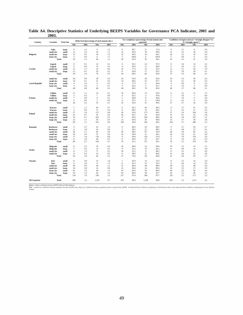
Table A4. Descriptive Statistics of Underlying BEEPS Variables for Governance PCA Indicator, 2001 and 2003.

Obs 2001 Obs 2003 Obs 2001 Obs 2003 Obs 2001 Obs 2003

Sofia large 9 1.3 6 1.2 9 86.7 8 75.6 9 3.1 8 2.9small city small 12 2.5 16 1.1 12 90.4 18 89.4 13 3.2 18 2.9small city large 15 0.5 18 1.2 15 96.0 18 94.2 18 3.2 19 3.0large city large 3 0.0 6 1.7 3 100.0 6 100.0 3 4.0 6 3.0

39 1.3 46 1.2 39 92.4 50 90.2 43 3.2 51 3.0

Zagreb small 8 0.1 14 0.1 8 93.1 14 97.9 8 3.6 14 4.1Zagreb large 5 0.0 13 0.2 4 95.0 11 88.6 5 3.0 13 4.2

small city small 13 2.7 25 0.6 10 77.5 22 93.2 12 3.1 24 3.9small city large 12 0.1 18 0.1 8 93.8 17 93.2 12 3.9 18 4.1

38 1.0 70 0.3 30 88.3 64 93.4 37 3.5 69 4.1

small city small 26 0.9 38 0.4 23 93.0 39 83.6 19 3.4 39 3.0small city large 16 0.1 21 0.2 14 90.6 22 87.7 13 4.1 20 3.3large city small 4 1.0 6 0.2 4 77.5 6 90.8 4 4.0 6 3.3large city large 3 3.4 3 0.1 3 83.3 3 92.7 4 3.5 3 4.0

49 0.8 68 0.3 44 90.2 70 85.9 40 3.7 68 3.1

Tallinn small 11 1.1 14 0.1 10 89.4 12 95.8 9 3.2 11 3.7Tallinn large 3 0.3 7 0.0 4 92.5 5 95.8 5 3.6 7 4.0

small city small 7 0.0 9 0.1 5 96.8 8 96.8 7 3.9 9 4.0small city large 5 0.0 3 0.0 4 97.5 6 100.0 6 4.2 6 3.8

26 0.5 33 0.1 23 93.0 31 96.9 27 3.7 33 3.9

Warsaw small 7 1.1 46 0.7 9 92.2 46 89.3 9 3.7 41 3.5Warsaw large 3 0.0 11 0.4 6 98.3 12 89.2 5 3.2 11 3.2

small city small 27 1.6 172 0.8 26 91.9 173 90.5 27 3.4 164 3.4small city large 33 0.7 55 0.4 30 95.7 55 94.9 33 4.1 53 3.8large city small 16 0.7 203 0.5 17 85.9 204 88.6 16 3.8 191 3.1large city large 13 1.7 36 0.3 12 94.6 36 96.8 14 3.7 36 3.8

99 1.1 523 0.6 100 92.8 526 90.5 104 3.7 496 3.3

Romania Bucharest small 9 4.7 25 1.5 9 88.3 30 89.5 9 3.7 29 3.7Bucharest large 4 1.8 16 0.6 3 98.3 22 98.2 4 4.0 22 4.1small city small 30 2.7 83 0.6 29 88.6 87 93.9 28 3.8 85 3.2small city large 20 2.0 51 0.4 16 94.4 51 94.1 20 3.9 51 3.8large city small 9 3.4 116 0.8 9 94.4 126 91.9 9 2.9 129 3.6large city large 8 1.8 48 0.5 8 90.0 55 93.7 8 3.6 54 3.9

80 2.7 339 0.7 74 91.1 371 93.1 78 3.7 370 3.6

Belgrade small 8 2.5 10 0.4 10 80.0 14 90.0 10 3.2 14 3.1Belgrade large 7 0.5 13 0.3 8 81.3 14 83.2 8 4.0 14 3.8small city small 8 1.3 9 0.1 10 63.5 9 88.3 11 4.1 9 4.0small city large 11 0.2 14 0.5 9 90.0 21 86.6 12 4.6 22 3.8

34 1.0 46 0.3 37 78.2 58 86.9 41 4.0 59 3.7

Ukraine Kiev small 8 4.9 14 1.8 7 92.9 14 74.3 8 2.5 14 3.0Kiev large 9 3.0 11 1.5 8 81.3 12 92.5 9 4.0 14 3.5

small city small 30 0.9 40 1.2 27 86.6 48 88.0 28 3.2 48 3.6small city large 16 0.8 14 0.9 14 96.4 16 89.4 16 3.5 17 3.9large city small 41 2.5 44 1.5 41 85.6 50 86.0 44 3.2 50 3.4large city large 30 1.4 26 2.2 30 86.6 28 93.7 30 3.1 28 3.2

134 1.9 149 1.5 127 87.4 168 87.7 135 3.2 171 3.5

All Countries 499 1.5 1,274 0.7 474 89.4 1,338 90.8 505 3.5 1,317 3.5

LocationCountry

Note : A small city is defined as having a population less than 250,000, and a large city is defined as having a population equal to or greater than 250,000. A small-sized firm is defined as employing 2 to 49 full-time workers, and a large-sized firm is defined as employing 50 or more full-timeworkers.

Confidence in legal system (1=“strongly disagree” to 6=“strongly agree”)

Source : Authors' calculations based on BEEPS 2002 and 2005 databases.

Total

Serbia

Czech Republic

Estonia

Poland

Total

Tax compliance (percentage of total annual sales reported)

Bribe level (percentage of total annual sales )

Total

Total

Total

Croatia

Firm Size

Total

Bulgaria

Total

Total

Total

49

Table A5. Descriptive Statistics of Underlying BEEPS Variables for Labor Market Flexibility PCA Indicator, 2001 and 2003.

Obs 2001 Obs 2003 Obs 2001 Obs 2003 Obs 2001 Obs 2003

Sofia large 9 33.3 8 50.0 9 -1.9 8 -1.5 9 2.4 8 2.3small city small 13 30.8 18 33.3 13 15.6 18 -1.9 13 3.1 18 2.9small city large 18 16.7 19 5.3 18 -0.5 17 -1.5 18 3.4 19 3.1large city large 3 0.0 6 0.0 3 -4.3 6 0.5 3 4.0 6 3.3

43 23.3 51 21.6 43 3.8 49 -1.4 43 3.1 51 2.9

Zagreb small 8 50.0 14 57.1 8 12.3 14 0.8 8 3.6 14 3.5Zagreb large 4 25.0 13 30.8 3 5.1 13 -1.4 5 2.8 13 3.5

small city small 10 50.0 22 27.3 11 84.5 22 -1.2 13 3.6 25 3.8small city large 11 36.4 17 29.4 10 2.2 18 -5.4 12 3.2 18 3.2

33 42.4 66 34.8 32 33.3 67 -2.0 38 3.4 70 3.5

small city small 25 12.0 39 41.0 27 0.9 37 0.4 24 3.1 40 2.5small city large 13 0.0 22 13.6 15 -0.8 22 2.6 16 2.9 22 2.0large city small 4 0.0 6 16.7 4 5.3 6 0.0 4 3.0 6 2.8large city large 4 25.0 3 0.0 4 2.5 3 0.2 3 3.0 3 3.0

46 8.7 70 28.6 50 0.9 68 1.1 47 3.0 71 2.4

Tallinn small 10 30.0 14 14.3 10 6.2 14 -0.7 11 3.2 14 2.4Tallinn large 4 0.0 7 0.0 5 -1.3 7 0.7 5 3.0 7 2.1

small city small 6 16.7 10 20.0 5 2.5 11 0.4 7 3.4 10 2.3small city large 5 20.0 8 12.5 3 5.5 8 0.6 7 3.1 8 1.9

25 20.0 39 12.8 23 3.7 40 0.1 30 3.2 39 2.2

Warsaw small 8 25.0 46 52.2 10 19.5 46 -11.5 10 2.5 44 2.8Warsaw large 7 14.3 12 8.3 7 -0.3 10 -2.8 7 2.4 12 2.6

small city small 27 18.5 173 39.3 28 -0.2 173 -0.4 28 2.4 172 2.6small city large 31 19.4 55 14.5 35 1.2 54 0.6 35 2.3 55 2.6large city small 16 25.0 205 35.6 18 22.0 204 3.4 18 2.3 202 2.5large city large 15 40.0 36 11.1 14 -3.6 35 -0.3 15 2.0 36 2.2

104 23.1 527 33.8 112 5.1 522 0.2 113 2.3 521 2.5

Romania Bucharest small 9 55.6 30 33.3 9 -2.0 30 1.0 9 3.1 30 2.9Bucharest large 3 33.3 22 13.6 4 -8.2 22 -1.9 4 3.5 22 2.7small city small 30 43.3 93 29.0 30 -2.0 90 2.4 29 2.9 90 2.9small city large 19 31.6 53 24.5 19 -2.8 53 -1.2 19 3.6 52 2.7large city small 9 22.2 131 38.2 9 -11.6 128 -1.4 9 3.0 128 2.5large city large 8 25.0 55 21.8 8 -0.9 52 -3.1 8 3.0 54 2.5

78 37.2 384 29.9 79 -3.5 375 -0.5 78 3.1 376 2.7

Belgrade small 12 16.7 13 38.5 12 11.3 14 -14.4 12 3.1 13 2.8Belgrade large 8 12.5 14 28.6 9 -1.0 12 -0.2 9 2.7 14 3.0small city small 13 61.5 8 37.5 10 -86.6 9 0.4 11 3.1 8 2.5small city large 12 16.7 23 34.8 11 -1.3 20 -1.0 12 2.8 23 2.3

45 28.9 58 34.5 42 -17.9 55 -4.0 44 2.9 58 2.6

Ukraine Kiev small 8 12.5 14 71.4 8 9.7 13 -0.5 7 3.4 13 3.6Kiev large 9 11.1 15 33.3 9 2.1 14 0.8 9 3.6 15 3.5

small city small 31 32.3 48 41.7 31 -13.6 41 10.7 29 3.1 48 3.1small city large 16 12.5 17 23.5 15 4.5 16 -31.6 16 3.1 17 3.2large city small 44 50.0 52 28.8 44 12.7 46 -2.9 43 3.0 51 3.5large city large 30 10.0 31 16.1 31 -3.0 27 0.5 31 3.1 31 2.9

138 28.3 177 33.3 138 1.5 157 -1.2 135 3.1 175 3.2

All Countries 512 27.0 1,372 31.4 519 2.1 1,333 -0.5 528 2.9 1,361 2.7

LocationCountry

Total

Bulgaria

Total

Total

Total

Change in temporary workers/permanent workers over last 3 years

Underemployment/overemployment (percentage of firms)

Total

Total

Total

Croatia

Firm Size

Note : A small city is defined as having a population less than 250,000, and a large city is defined as having a population equal to or greater than 250,000. A small-sized firm is defined as employing 2 to 49 full-time workers, and a large-sized firm is defined as employing 50 or more full-timeworkers.

Labor regulations as a constraint (1=“major obstacle” to 4=“no obstacle”)

Source : Authors' calculations based on BEEPS 2002 and 2005 databases.

Total

Serbia

Czech Republic

Estonia

Poland

Total

50

Table A6. Descriptive Statistics of Underlying BEEPS Variables for Labor Quality PCA Indicator, 2001 and 2003.

Obs 2001 Obs 2003 Obs 2001 Obs 2003 Obs 2001 Obs 2003

Sofia large 9 83.3 8 81.0 6 4.2 7 5.8 9 3.0 8 3.0small city small 13 76.3 18 83.2 8 2.0 12 2.1 13 3.1 18 2.8small city large 18 73.6 19 71.6 15 2.7 16 2.6 18 3.4 19 2.7large city large 3 62.7 6 75.0 3 2.3 6 3.4 3 4.0 6 2.8

43 75.7 51 77.5 32 2.8 41 3.1 43 3.3 51 2.8

Zagreb small 8 81.9 14 78.5 6 4.9 6 4.4 8 3.0 14 3.5Zagreb large 5 74.4 13 63.6 2 4.2 9 4.2 5 2.8 13 3.2

small city small 13 93.5 25 88.4 6 3.1 14 9.9 12 3.3 25 3.1small city large 12 74.8 18 71.0 11 6.9 16 4.9 12 2.8 18 2.9

38 82.6 70 77.3 25 5.3 45 6.3 37 3.0 70 3.2

small city small 28 86.1 26 81.5 15 5.1 15 3.6 26 3.1 38 2.7small city large 14 74.9 17 74.8 11 5.3 15 4.5 16 2.4 21 2.6large city small 4 80.0 6 75.8 3 9.3 5 1.8 4 3.3 6 3.5large city large 4 81.5 3 57.7 4 5.8 3 3.4 4 3.0 3 2.3

50 82.1 52 77.3 33 5.7 38 3.7 50 2.9 68 2.7

Tallinn small 11 90.3 14 81.2 10 5.7 5 2.8 11 2.5 14 3.4Tallinn large 5 72.0 7 64.1 5 6.1 6 5.9 4 2.5 7 3.3

small city small 7 72.4 11 75.9 4 5.0 8 7.8 7 2.1 11 3.0small city large 7 68.3 7 81.1 6 4.4 7 3.8 7 1.6 8 2.9

30 77.9 39 76.6 25 5.4 26 5.3 29 2.2 40 3.2

Warsaw small 10 84.9 46 92.2 2 3.5 31 3.2 10 3.0 46 2.9Warsaw large 7 86.4 12 78.6 5 6.1 10 2.8 7 3.3 12 2.9

small city small 27 86.7 173 90.2 14 2.4 75 3.2 28 2.5 172 2.8small city large 35 85.2 54 77.6 23 5.6 36 3.2 35 2.7 55 2.9large city small 18 92.1 205 90.9 9 3.1 118 3.5 18 2.6 204 2.6large city large 15 81.0 36 85.6 7 3.0 29 3.6 15 2.7 36 2.6

112 86.2 526 88.8 60 4.1 299 3.4 113 2.7 525 2.7

Romania Bucharest small 9 86.0 30 81.6 7 3.7 24 3.1 9 3.6 30 2.6Bucharest large 4 84.5 22 78.7 4 4.8 20 3.2 4 3.3 22 2.6small city small 29 74.1 92 76.4 21 3.0 62 2.1 30 3.0 93 3.0small city large 20 79.9 53 77.4 12 9.8 41 2.5 19 3.1 51 2.9large city small 9 91.2 131 85.9 6 5.2 97 2.4 9 3.0 128 2.6large city large 8 87.9 55 81.8 6 3.0 44 2.6 8 3.1 54 2.5

79 80.8 383 81.1 56 4.9 288 2.5 79 3.1 378 2.7

Belgrade small 12 85.3 14 90.1 2 4.0 6 5.0 12 3.3 13 3.6Belgrade large 10 80.9 13 73.6 7 2.5 9 5.3 10 3.6 14 3.2small city small 13 82.5 9 63.9 6 2.3 6 4.3 11 2.7 9 3.0small city large 12 59.2 22 75.3 5 2.4 13 4.7 11 2.9 23 2.8

47 76.9 58 76.7 20 2.6 34 4.8 44 3.1 59 3.1

Ukraine Kiev small 8 88.0 14 71.3 6 6.6 12 3.6 8 3.4 13 2.2Kiev large 9 71.6 15 82.1 8 5.3 15 8.6 9 2.8 15 3.1

small city small 31 88.5 48 81.5 21 5.6 28 3.9 31 2.8 48 2.8small city large 16 75.0 17 82.8 15 9.1 15 4.4 16 2.8 17 2.5large city small 42 90.4 53 83.6 34 4.8 42 5.9 44 2.7 53 2.7large city large 30 85.7 31 76.6 26 8.3 27 5.3 31 2.5 31 2.5

136 85.7 178 80.7 110 6.5 139 5.3 139 2.7 177 2.7

All Countries 535 82.5 1,357 83.3 361 5.1 910 3.6 534 2.9 1,368 2.8

LocationCountry

Note : A small city is defined as having a population less than 250,000, and a large city is defined as having a population equal to or greater than 250,000. A small-sized firm is defined as employing 2 to 49 full-time workers, and a large-sized firm is defined as employing 50 or more full-timeworkers.

Labor quality\ as a constraint (1=“major obstacle” to 4=“no obstacle”)

Table A6. Descriptive Statistics of Underlying BEEPS Variables for Labor Quality PCA Indicator, 2001 and 2003.

Source : Authors' calculations based on BEEPS 2002 and 2005 databases.

Total

Serbia

Czech Republic

Estonia

Poland

Total

Time to fill vacancy for skilled worker (weeks)Skilled workers/total employees (percentage)

Total

Total

Total

Croatia

Firm Size

Total

Bulgaria

Total

Total

Total

51