1

WHAT DRIVES PRICE DISPERSION AND MARKET

FRAGMENTATION ACROSS U.S. STOCK EXCHANGES?*

YONG CHAO

CHEN YAO

MAO YE

We propose a theoretical model to explain two salient features of the U.S. stock

exchange industry: (i) the proliferation of stock exchanges offering identical transaction

services; and (ii) sizable dispersion and frequent changes in stock exchange fees, highlighting

the role of discrete pricing. Exchange operators in the United States compete for order flow by

setting “make” fees for limit orders (“makers”) and “take” fees for market orders (“takers”).

When traders can quote continuous prices, the manner in which operators divide the total fee

between makers and takers is inconsequential because traders can choose prices that perfectly

counteract any fee division. If such is the case, order flow consolidates on the exchange with

the lowest total fee. The one-cent minimum tick size imposed by the U.S. Securities and

Exchange Commission’s Rule 612(c) of Regulation National Market Systems for traders

prevents perfect neutralization and eliminates mutually agreeable trades at price levels within

a tick. These frictions (i) create both scope and incentive for an operator to establish multiple

exchanges that differ in fee structure in order to engage in second-degree price discrimination;

and (ii) lead to mixed-strategy equilibria with positive profits for competing operators, rather

than to zero-fee, zero-profit Bertrand equilibrium. Policy proposals that require exchanges to

charge one side only or to divide the total fee equally between the two sides would lead to zero

make and take fees, but the welfare effects of these two proposals are mixed under tick size

constraints.

JEL Codes: G10 G20

* We thank Jim Angel, Robert Battalio, Dan Bernhardt, Eric Budish, John Campbell, Rohan Christie-David, Laura Cardella, Adam Clark-Joseph, Jean Colliard, Shane Corwin, Thierry Foucault, Amit Goyal, Andrei Hagiu, Larry Harris, Terry Hendershott, Chong Huang, Ohad Kadan, Charles Kahn, Hong Liu, Guillermo Marshall, Nolan Miller, Artem Neklyudov, Shawn O’Donoghue, Andreas Park, Ioanid Rosu, Alvin Roth, Richard Schmalensee, Chester Spatt, Alexei Tchistyi, Glen Weyl, Julian Wright, Bart Yueshen Zhou, Jidong Zhou, Haoxiang Zhu, and seminar participants at the Harvard Economics Department/Harvard Business School, Baruch College, the University of Notre Dame, the University of Warwick, the University of Illinois at Urbana Champaign, Washington University at St. Louis, HEC Lausanne, and École Polytechnique Fédérale de Lausanne for their suggestions. This research is supported by National Science Foundation grant 1352936. We also thank Xin Wang, Bei Yang, Fan Yang, and Sida Li for their excellent research assistance. Corresponding author, Mao Ye: Finance Department, 1206 South Sixth Street, University of Illinois at Urbana-Champaign, Champaign IL 61820; Telephone: (217) 244-0474; Fax: (217)-244-3102; Email: maoye@illinois.edu

2

I. INTRODUCTION

Currently, stock prices are determined in stock exchanges through interactions between

buyers and sellers. All stock exchanges in the U.S. are for-profit institutions that charge fees

for transactions. In most finance models, however, stock exchanges either have no explicit role

or make no economic profits in equilibrium. How do stock exchanges set their service fees?

How does fee competition among stock exchanges shape the organization of the industry? In

this paper, we propose a theoretical model to examine the role of discrete pricing in creating

two salient features of the U.S. stock exchange industry. Violation of the “law of one price.” Figure I shows the fee structures in ten major U.S.

stock exchanges in May 2015. Fees differ across competing exchanges as well as across

exchanges owned by the same holding company (hereafter “operator”). Frequent fee changes

add to the complexity, as “the pressure to establish novel and competitive pricing often leads

exchanges to modify their pricing frequently, typically on a calendar-month basis” (U.S.

Security and Exchanges Commission (SEC) 2015, p. 21). Such spatial and temporal dispersion

of prices can hardly be justified by physical product differentiation, as these exchanges are so

similar that the SEC even refers to some of them as “cloned markets” (SEC 2015, p. 22). All

stock exchanges in the United States are organized as electronic limit-order markets and a stock

can be traded on any of them.1 A trader can act as a liquidity maker by posting a limit order

with a specified price and quantity. A trade occurs once another trader (a liquidity taker) accepts

the terms of a previously posted limit order through a market order. Upon execution, the

exchanges charge a “make” fee and a “take” fee per share to each side of the transaction, the

sum of which, the so-called “total” fee, is a major source of exchanges’ revenues.2

[Insert Figure I about here]

Market fragmentation. Another puzzle is the proliferation of stock exchanges that

offer almost identical services. Figure I demonstrates the market fragments along two

dimensions: (i) multiple operators co-exist; and (ii) each operator offers multiple stock

exchanges. The principle of tax-neutrality asserts that, at a given tax level, it does not matter

who—buyer or seller—is liable for the tax. Therefore, all traders would choose the exchange

with the lowest total fee. This prediction raises the question why an operator establishes

1 Unlisted trading privileges in the U.S. allow stocks to be traded outside the listing venue. 2 For example, BATS reported in its filing for an IPO in 2015 that about 70% of its revenues come from transaction fees (p. F4 on BATS S1 registration statement). O’Donoghue (2015) estimates that 34.7% of the NASDAQ’s net income is from the fees.

3

multiple exchanges to trade the same assets. Furthermore, competition over the total fee among

operators should lead to Bertrand equilibrium, resulting in a zero total fee and zero profit, and

leaving no room for market entry with any fixed cost to establish an exchange. Yet new entries

are commonly observed. For example, on October 22, 2010, BATS created a new stock

exchange, BATS Y, in addition to its existing BATS X exchange.

These puzzles have drawn attention from regulators, and a plan to ban the maker/taker

pricing model is under discussion (SEC 2015). Yet relevant studies have provided limited

theoretical understanding about what drives complex fee structures and the proliferation of

exchanges that adopt them.

We show that one driving force behind price dispersion and market fragmentation is

the discrete tick size. 3 In this paper, we consider a game among exchange operator(s), a

continuum of liquidity makers and liquidity takers with heterogeneous valuations. When

liquidity makers can quote continuous prices, they are able to neutralize the make/take fee

allocations by adjusting their quotes. Then they always choose the exchange with the lowest

total fee. As a result, no operator has incentives to offer multiple exchanges, and the

competition over the total fee between operators leads to Bertrand equilibrium. Although these

predictions are consistent with canonical economic principles, they are inconsistent with the

stylized facts.

We next consider the case in which liquidity makers can propose only discrete trading

prices. This setup is motivated by SEC Rule 612(c) of Regulation National Market Systems

(NMS), which restricts the pricing increment to a minimum of $0.01 if the security is priced

equal to or greater than $1.00 per share.4 Although liquidity makers cannot quote sub-penny

prices, the make/take fees are not subject to the tick size constraints. Stock exchanges can use

make/take fees to effectively propose sub-penny transaction prices that cannot be neutralized

by liquidity makers. As a result, the discrete tick size changes the nature of price competition

between exchanges from one-sided (over the total fee) to two-sided (over the make fee and the

take fee).

Non-neutrality creates product differentiation for otherwise identical exchanges. All

else being equal, a liquidity maker prefers the exchange with a lower take fee because it

3 We are aware of other drivers for market fragmentation. Historically, the tick size used to be larger than one-cent. However, before stock exchanges moved to electronic platforms, the high fixed cost to establish a physical exchange was a barrier to entry. Also, high monitoring costs can outweigh the small fraction of a tick profit margin per trade for human traders. Computer-based trading reduced these monitoring cost. There are trading algorithms which profit from fees by specializing in market making, and algorithms which seek to minimize transaction costs. 4 We discuss the exemptions from this rule in Section IX.

4

increases the probability that a liquidity taker will accept her offer. Therefore, exchanges with

lower take fees are of higher “quality” to liquidity makers. From the point of the view of a

liquidity maker, an operator’s choice between make and take fees is equivalent to simultaneous

choices about the price of the execution service (the make fee) and the quality of the execution

service (the take fee).

This product differentiation then facilitates second-degree price discrimination.

Discrete price can force liquidity makers with heterogeneous valuations to propose the same

limit-order price. The operator then can open multiple exchanges with differentiated make/take

fees to screen liquidity makers. Liquidity makers with larger (smaller) gains from execution

select the exchanges with higher (lower) prices and higher (lower) execution probabilities. We

show that such second-degree price discrimination increases not only the operator’s profit but

also the welfare of both liquidity makers and liquidity takers, because new exchanges create

more effective transaction prices.

Choosing price and quality simultaneously destroys Bertrand equilibrium as well as any

pure-strategy equilibrium. Consider a simple case of duopoly operators, each opening one

exchange. No pure-strategy equilibrium exists when any operator charges a positive total fee,

because competing operators have incentives to undercut each other toward zero total fees.

Surprisingly, no pure-strategy equilibrium exists even when both operators charge zero total

fees. If one operator charges a zero total fee, the other operator has two types of profitable

deviation. One type increases the charge to liquidity makers by 𝜀𝜀 while decreasing the charge

to liquidity takers by 𝜇𝜇 ∙ 𝜀𝜀 (0 < 𝜇𝜇 < 1). This deviation reduces gains from execution but

increases execution probability, which attracts liquidity makers with high gains from execution.

The other type of deviation decreases the charge to liquidity makers while increasing the charge

to liquidity takers, which appeals to liquidity makers with low gains from execution. We also

show the non-existence of pure-strategy equilibrium when we allow operators to choose the

number of exchanges, because operators can implement the fee structure mentioned above by

establishing new exchanges.

We then prove the existence of symmetrical mixed-strategy equilibrium, and we show

that any mixed-strategy equilibrium entails positive profits. As in Varian (1980), the fact that

only mixed-strategy equilibrium exists rationalizes the spatial price dispersion (exchanges have

different fees at the same time) and the temporal price dispersion (exchanges vary their fees

over time). The driver of the mixed-strategy equilibrium in our paper, however, differs from

that of the mixed strategy equilibrium in the one-dimensional price competition. When firms

compete over one price, the violation of the law of one price is driven either by the cost to

5

consumers to obtain the prices (Rosenthal 1980; Varian 1980; Burdett and Judd 1983) or by

the cost to firms to advertise their prices (Butters 1977; Baye and Morgan 2001). Our model

does not include market frictions to react or transmit prices. The driver of the mixed-strategy

equilibrium is the inability to rank prices uniquely in a two-dimensional space.

To the best of our knowledge, we are the first to rationalize exchange fee dispersion

and frequent fee changes, as documented by O’Donoghue (2015) and Cardella, Hao, and

Kalcheva (2015). Colliard and Foucault (2012) predict that competition between exchanges

leads to zero total fees. Two other extant interpretations shed light on the existence of rebates

(negative fees), but they cannot explain why trading does not consolidate on the market with

the maximum rebate. The first interpretation is that rebates to liquidity makers encourage

liquidity provision (Malinova and Park 2015; Cardella, Hao, and Kalcheva 2015), which in

turn attracts liquidity takers. Yet this interpretation cannot explain why new entries to the

exchange industry, such as Direct Edge A and BATS Y, charge positive fees to liquidity makers.

The second interpretation maintains that retail brokers have incentives to route customer orders

to markets with the highest rebates, as brokers do not need to pass the rebates on to their

customers (Angel, Harris, and Spatt 2010, 2013; Battalio, Corwin, and Jennings 2015). But this

interpretation does not explain why exchanges do not simply copy the highest rebate set by

their competitors.

Our paper also contributes to the literature on market fragmentation. The fragmentation

of stocks trading has recently become a focus of research interest, because market

fragmentation affects liquidity and price discovery (O’Hara and Ye 2011), leads to mechanical

arbitrage opportunities for high frequency traders (Budish, Cramton, and Shim 2015; Foucault,

Kozhan, and Tham 2015), and can serve as a driver of systemic risk, such as the “Flash Crash”

of 2010 (Madhavan 2012). However, it is not clear why markets fragment in the first place, as

the literature generally predicts consolidation of trading due to network externality or

economies of scale (e.g., Stigler 1964; Pagano 1989; Chowdhry and Nanda 1991; Biais,

Glosten, and Spatt 2005). The tick size channel in our paper explains market fragmentation

both within the same operator and across operators. To our knowledge, no existing theoretical

model explains why an operator has economic incentive to establish multiple stock exchanges.

Foucault (2012) conjectures that the co-existence of various make/take fees on exchanges

operated by the same operator should serve to screen investors by type. However, Foucault

also mentions that “it is not clear however how the differentiation of make/take fees suffices to

screen different types of investors since, in contrast to payments for order flow, liquidity

rebates are usually not contingent on investors’ characteristics (e.g., whether the investor is a

6

retail investor or an institution)” (Foucault 2012, p. 20).5 We address this puzzle: when end

users cannot neutralize the breakdown of the total fee, the operators can screen liquidity makers

based on the terms of trade offered to liquidity takers. Discrete tick size also provides a new

interpretation of market fragmentation across operators. Researchers examining the co-

existence of operators either assume exogenous operators, or rely on differentiated services or

switching costs.6 We contribute to the literature by showing that exchanges can endogenously

co-exist in the absence of physical product differentiation or switching costs.

Our modeling choice is inspired by the characteristics of stock markets, but its

economic forces also shed light on other types of competition. Because SEC Rule 612(c)

applies to displayed quotes, it is possible to create sub-penny pricing by designing either hidden

order types or alternative trading systems (ATS), commonly referred to as “dark pools.” In this

sense, the existence of a tick size sheds light on the proliferation of new order types and dark

pools. We also contribute to the burgeoning literature on two-sided markets. Rochet and Tirole

(2006, p. 646) define two-sided markets as those in which “the volume of transactions between

end-users depends on the structure and not only on the overall level of the fees charged by the

platform.” A fundamental question is whether the two-sided markets that Rochet and Tirole

(2006) define can generate qualitatively different predictions from one-sided markets with

identical setups.7 We fill in this gap in the literature by showing that non-neutrality creates

product differentiation among intrinsically homogeneous exchanges, which, in turn, creates

price dispersion and leads to market fragmentation. Finally, Shaked and Sutton (1982) and

Tirole (1988) predict the occurrence of non-Bertrand pure-strategy equilibrium when quality

is chosen before price in a game. In our model, the “qualities” of the exchanges for liquidity

makers are determined by the take fees, which can be adjusted as easily as the make fees. Such

simultaneous choices of price and quality can lead to mixed-strategy equilibrium.

Besides rationalizing existing stylized facts pertaining to fee competition, our paper

predicts the market outcomes of two alternative fee structures if policymakers were to ban the

maker/taker pricing model: (i) charging fees only to one side; and (ii) distributing fees equally

between two sides. We show that both proposals would reduce price competition to one

dimension, which could drive the make fee, the take fee, and the exchange’s profit toward zero.

5 Since 2012, more exchanges have begun offering higher rebates to retail order flow, which can be another source of price discrimination. 6 For models based on exogenous exchanges, see Glosten (1994), Parlour and Seppi (2003) and Foucault and Menkveld (2008). For product differentiation, see Pagnotta and Philippon (2015), Santos and Scheinkman (2001), Foucault and Parlour (2004), and Baldauf and Mollner (2015). For switching costs, see Cantillon and Yin (2008). 7 For alternative definitions of two-sided markets, see Rysman (2009), Hagiu and Wright (2015), and Weyl (2010).

7

Operators for traditional exchanges can survive short-run zero profit from make/take fees using

other revenue sources, such as stock listings, but operators for the new exchanges do not have

the same buffer. This provides one economic interpretation of why NYSE asks the regulator to

ban the maker/taker pricing model, 8 but BATS aggressively opposes such a proposal. 9

Interestingly, we find that there are mixed welfare effects of banning the maker/taker pricing

model. It could reduce welfare if liquidity makers’ and liquidity takers’ valuations were within

the same tick, but increase welfare if their valuations were separated by price grids.

On April 5, 2012, Congress passed the Jumpstart Our Business Startups (JOBS) Act.

Section 106 (b) of the act requires the SEC to examine the effect of tick size on initial public

offerings (IPOs). A pilot program to increase tick size to five cents for small- and mid-cap

stocks is to be implemented on May 15, 2016. Proponents of the proposal argue that a large

tick size might increase market-making profit and support sell-side equity research and,

eventually, increase the number of IPOs (Weild, Kim, and Newport 2012). We doubt the

existence of such an economic channel. Even if it were to exist, we believe that a more direct

consequence of increased nominal tick size would be more aggressive fee competition between

exchanges to create effective price levels within the tick.

This article is organized as follows. In Section II, we describe the model. In Section III,

we present the benchmark model in which the tick size is zero. In Section IV, we demonstrate

the non-neutrality of the fee structure when there are tick size constraints. In Section V, we

show product differentiation and liquidity makers’ segmentation into multiple exchanges. In

Section VI, we show price discrimination under monopoly. In Section VII, we derive the non-

existence of pure-strategy equilibrium under competing operators. In Section VIII, we discuss

the robustness of our model predictions. In Section IX, we discuss the policy implications of

our model. We conclude in Section X and discuss the broader economic implications of our

model. All proofs are presented in the Appendix.

8 See Jeffrey Sprecher, Chairman and Chief Executive Officer of Intercontinental Exchange, and owner of New York Stock Exchange, Statement to the U.S. Senate Banking, Housing and Urban Affairs Committee, Hearing on “The Role of Regulation in Shaping Equity Market Structure and Electronic Trading,” on July 8, 2014, available at:http://www.banking.senate.gov/public/index.cfm?FuseAction=Hearings.Hearing&Hearing_ID=2e98337f-d5c5-490f-80e7-6c1c81af7243. 9 See Joe Ratterman, Chief Executive Officer, and Chris Concannon, President, of BATS, “Open Letter to U.S. Securities Industry Participants Re: Market Structure Reform Discussion,” on January 6, 2015, available at http://cdn.batstrading.com/resources/newsletters/OpenLetter010615.pdf.

8

II. MODEL

We consider a three-period game between three types of risk-neutral players: exchange

operator(s), a continuum of liquidity makers with valuation of a stock 𝑣𝑣𝑏𝑏 uniformly distributed

on [12

, 1] and liquidity takers with valuation of the stock 𝑣𝑣𝑠𝑠 uniformly distributed on �0, 12�. 𝑣𝑣𝑏𝑏

and 𝑣𝑣𝑠𝑠 , respectively, are the liquidity makers’ and liquidity takers’ private information.

Because liquidity makers have higher valuations than liquidity takers, the former intend to buy

from the latter.10

We consider both a monopoly operator and competition between operators. Figure II

demonstrates the actions available to players arriving in each period. At Date 0, operators

simultaneously choose the number of exchanges to establish and set the make fee 𝑓𝑓𝑚𝑚𝑖𝑖 and the

take fee 𝑓𝑓𝑡𝑡𝑖𝑖 on each exchange 𝑖𝑖 to maximize their expected profits. Fees are charged upon order

execution, and a negative fee means a rebate for the trader. At Date 1, nature randomly draws

one liquidity maker from the uniform distribution[12

, 1] . The liquidity maker makes two

decisions after observing the fee structures: (i) submitting a limit order of one share to exchange

𝑖𝑖 or to no exchange at all; and (ii) proposing the limit order at price 𝑃𝑃𝑖𝑖 if she chooses exchange 𝑖𝑖.

The liquidity maker aims to maximize her expected surplus:

𝐵𝐵𝐵𝐵𝑖𝑖�𝑃𝑃𝑖𝑖; 𝑣𝑣𝑏𝑏� ≡ �𝑣𝑣𝑏𝑏 − 𝑃𝑃𝑖𝑖 − 𝑓𝑓𝑚𝑚𝑖𝑖 � ∙ Pr�𝑣𝑣𝑠𝑠 ≤ 𝑃𝑃𝑖𝑖 − 𝑓𝑓𝑡𝑡𝑖𝑖�.

The first term of the expected surplus is the liquidity maker’s gains from execution, and the

second term reflects the probability of the liquidity taker accepting the limit order. We make a

technical assumption that the liquidity maker cannot submit “stub-quotes,” that is, a limit-order

price so low that no liquidity taker accepts it. 11 The liquidity maker submits no limit order if

her maximal expected surplus is negative for any limit-order price in any exchange. At Date 2,

nature randomly draws one liquidity taker from the uniform distribution �0, 12�. The liquidity

taker chooses to accept or decline the limit order at the exchange chosen by the liquidity

maker.12 She accepts the limit order if her surplus is non-negative after paying the limit order

10 When the liquidity maker intends to sell to the liquidity taker, our model predictions do not change, given that traders’ valuations are symmetric and uniformly distributed. 11 Stub quotes lead mechanically to zero expected surplus. The SEC, however, prohibits market maker stub quotes. See https://www.sec.gov/news/press/2010/2010-216.htm. 12 In practice, an exchange charges a fee to route a market order to another exchange. This routing fee imposes a barrier to submitting an order to a low take-fee exchange aiming to interact with a limit order in a high take-fee exchange for the purpose of reducing the trading cost. For an example of a routing fee, see: https://www.batstrading.com/support/fee_schedule/edga/.

9

price and the take fee. The exchange where the trade occurs profits from the total fee, the sum

of the make fee and the take fee.

We determine the subgame-perfect equilibrium of the sequential-move game by

backward induction. First, we look for the probability that a liquidity taker accepts the limit

orders at price 𝑃𝑃𝑖𝑖 given the take fee 𝑓𝑓𝑡𝑡𝑖𝑖 , Pr�𝑣𝑣𝑠𝑠 ≤ 𝑃𝑃𝑖𝑖 − 𝑓𝑓𝑡𝑡𝑖𝑖� . Then, we study the liquidity

maker’s exchange choice and the optimal limit-order price 𝑃𝑃𝑖𝑖∗ to maximize her expected

surplus, given 𝑓𝑓𝑡𝑡𝑖𝑖 and 𝑓𝑓𝑚𝑚𝑖𝑖 and the liquidity taker’s best response at Date 2. The liquidity maker

chooses not to participate if her expected surplus is negative. Finally, given the probability of

participation based on the above subgames, a monopoly operator chooses the number of

exchanges and the associated fee structures to maximize its expected profit, while competing

operators choose the number of exchanges to establish and the associated fee structures

simultaneously such that those strategies form a Nash equilibrium.

[Insert Figure II about here]

Our main purpose is to model exchange competition, so our model is parsimonious with

respect to traders’ choices between limit and market orders: traders do not choose the order

type, and the limit-order book is empty when the liquidity maker arrives. 13 These two

assumptions follow from Menkveld (2010) and Foucault, Kadan, and Kandel (2013).14 Such

simplification of the limit-order book allows us to gain economic insights that extend beyond

the stock exchange industry; we discuss these implications in the Conclusion.

By proposing a nominal trading price 𝑃𝑃𝑖𝑖 to exchange 𝑖𝑖, the liquidity maker essentially

chooses the cum fee buy and sell prices to be 𝑝𝑝𝑏𝑏𝑖𝑖 ≡ 𝑃𝑃𝑖𝑖 + 𝑓𝑓𝑚𝑚𝑖𝑖 and 𝑝𝑝𝑠𝑠𝑖𝑖 ≡ 𝑃𝑃𝑖𝑖 − 𝑓𝑓𝑡𝑡𝑖𝑖. Under zero tick

size, 𝑃𝑃𝑖𝑖 can be any real number. Under a discrete tick size, 𝑃𝑃𝑖𝑖 can only be on price grids with

the minimum distance as tick size; we call such restrictions tick size constraints. Our baseline

model considers a tick size of 1, that is,

(1) 𝑃𝑃𝑖𝑖 ∈ {𝑛𝑛}, where n is an integer.

13 Theoretical studies on order-placing strategy generally provide a richer structure of order selection by assuming exogenous exchanges (Parlour and Seppi 2003; Foucault and Menkveld 2008; Rosu 2009). For example, Foucault and Menkveld (2008) find that two exogenous exchanges can co-exist because of queuing behavior. Our model, however, demonstrates the co-existence of endogenous trading exchanges. 14 In practice, the decision between making and taking liquidity is not so rigid. Yet it is evident that traders specialize in trading activities, creating differentiation. For example, high-frequency traders account for a large fraction of liquidity supply in electronic markets (Menkveld 2010; Foucault, Kadan, and Kandel 2013). Our model captures this feature.

10

Under this assumption, the valuations of the liquidity maker and the liquidity taker fall within

the same tick.

In Section VIII, we relax this assumption by allowing price to be any rational numbers

with equal space, that is,

(1′) �𝑃𝑃𝑖𝑖 ∈ 𝑛𝑛𝑁𝑁�, where n is an integer and N is a natural number.

The tick size under (1′) is 1𝑁𝑁

. When 𝑁𝑁 > 1, the support of traders’ valuation goes

beyond one tick.

Our main analysis focuses on 𝑁𝑁 = 1, or tick size constraints (1). In Section VIII, we

consider tick size constraints (1′) and demonstrate that our main results still hold for N>1.

III. BENCHMARK: NO TICK SIZE CONSTRAINTS

In this section, we analyze market outcomes when 𝑃𝑃𝑖𝑖 can be any real number. The

results in this section serve as the benchmark for future discussions when we incorporate tick

size constraints.

We solve the model through backward induction. At Date 2, a liquidity taker accepts a

limit order if 𝑣𝑣𝑠𝑠 ≤ 𝑃𝑃𝑖𝑖 − 𝑓𝑓𝑡𝑡𝑖𝑖, and the probability for the liquidity taker to accept the limit order

is Pr (𝑣𝑣𝑠𝑠 ≤ 𝑃𝑃𝑖𝑖 − 𝑓𝑓𝑡𝑡𝑖𝑖). At Date 1, a liquidity maker proposes a limit-order price to maximize her

expected surplus 𝐵𝐵𝐵𝐵𝑖𝑖�𝑃𝑃𝑖𝑖;𝑣𝑣𝑏𝑏�.

max𝑃𝑃𝑖𝑖

𝐵𝐵𝐵𝐵𝑖𝑖�𝑃𝑃𝑖𝑖;𝑣𝑣𝑏𝑏� = max𝑃𝑃𝑖𝑖

��𝑣𝑣𝑏𝑏 − 𝑃𝑃𝑖𝑖 − 𝑓𝑓𝑚𝑚𝑖𝑖 � ∙ max�0, min { 2 ∙ �𝑃𝑃𝑖𝑖 − 𝑓𝑓𝑡𝑡𝑖𝑖�, 1}��

We denote the total fee on exchange i as 𝑇𝑇𝑖𝑖 ≡ 𝑓𝑓𝑚𝑚𝑖𝑖 + 𝑓𝑓𝑡𝑡𝑖𝑖. The solution for the optimal

limit-order price is

(2) 𝑃𝑃𝑖𝑖∗(𝑣𝑣𝑏𝑏) =𝑣𝑣𝑏𝑏 + 𝑇𝑇𝑖𝑖

2− 𝑓𝑓𝑚𝑚𝑖𝑖 , if 𝑣𝑣𝑏𝑏 ≥ 𝑇𝑇𝑖𝑖 .

Equation (2) shows that the nominal limit-order price strictly increases in the liquidity

maker’s valuation when 𝑣𝑣𝑏𝑏 ≥ 𝑇𝑇𝑖𝑖 . The cum fee buy price and the cum fee sell price are

𝑝𝑝𝑏𝑏𝑖𝑖 (𝑣𝑣𝑏𝑏) = 𝑃𝑃𝑖𝑖 + 𝑓𝑓𝑚𝑚𝑖𝑖 = 𝑣𝑣𝑏𝑏+𝑇𝑇𝑖𝑖

2 and 𝑝𝑝𝑠𝑠𝑖𝑖(𝑣𝑣𝑏𝑏) = 𝑃𝑃𝑖𝑖 − 𝑓𝑓𝑡𝑡𝑖𝑖 = 𝑣𝑣𝑏𝑏−𝑇𝑇𝑖𝑖

2, respectively. Therefore, the

economic outcome is affected by the total fee 𝑇𝑇𝑖𝑖, and not by its breakdown into 𝑓𝑓𝑚𝑚𝑖𝑖 and 𝑓𝑓𝑡𝑡𝑖𝑖

under a zero tick size.

The neutrality of fee structures implies that all traders would rush to the exchange with

the lowest total fee. As a result, the monopoly operator cannot benefit from opening more than

11

one exchange. Also, competition among operators leads to Bertrand equilibrium. In Proposition

1, we posit the market outcomes without tick size constraints.

PROPOSITION 1 (market outcome under zero tick size). Under continuous pricing:

(i) only the total fee, not its breakdown, has effect on the market outcome for the three types

of players;

(ii) a monopoly operator has no incentive to open more than one exchange. The standing

exchange charges a total fee of 38 and earns a profit of 9

64;

(iii) competing operators set total fees at zero and earn zero profits.

Proposition 1 implies that we should not observe any price dispersion of total fees if

the tick size is zero. We should also expect consolidation with one operator on one exchange,

as long as establishing an exchange involves non-zero costs. Nevertheless, these predictions

are not consistent with the stylized facts. Next, we demonstrate that tick size constraints can

generate results that are dramatically different yet consistent with reality.

IV. NON-NEUTRALITY OF FEE STRUCTURES UNDER TICK SIZE

CONSTRAINTS

In this section, we show that the fee structure becomes non-neutral in the presence of

tick size constraints (1). In Section IV.A. we establish the results for one exchange. In Section

IV.B. we advance the non-neutrality intuition by showing that, with the same total fee but

inverting make and take fees, one exchange can dominate the other.

IV.A. Fee Structure under Tick Size Constraints: One Exchange

For a given limit-order price 𝑃𝑃, a trade occurs if and only if:

(3) � 0 ≤ 𝑣𝑣𝑠𝑠 ≤ 𝑝𝑝𝑠𝑠 = 𝑃𝑃 − 𝑓𝑓𝑡𝑡𝑝𝑝𝑏𝑏 = 𝑃𝑃 + 𝑓𝑓𝑚𝑚 ≤ 𝑣𝑣𝑏𝑏 ≤ 1

A necessary condition for the exchange to survive is a budget-balanced total fee,

𝑇𝑇 = 𝑓𝑓𝑚𝑚 + 𝑓𝑓𝑡𝑡 ≥ 0, which is equivalent to:

(4) 𝑃𝑃 − 𝑓𝑓𝑡𝑡 ≤ 𝑃𝑃 + 𝑓𝑓𝑚𝑚.

Thus, in order for a trade to occur, (3) and (4) together require:

(5) 0 ≤ 𝑣𝑣𝑠𝑠 ≤ 𝑃𝑃 − 𝑓𝑓𝑡𝑡 ≤ 𝑃𝑃 + 𝑓𝑓𝑚𝑚 ≤ 𝑣𝑣𝑏𝑏 ≤ 1.

For a trade to occur, the total fee set by the operator must be less than 1. Here we restrict

12

our attention to |𝑓𝑓𝑖𝑖| ≤ 1 (i=m,t) , because U.S. regulations prohibit any exchange from

charging fees greater than one tick.15 Lemma 1 establishes the result that the fee structure

matters in the presence of tick size constraints.

LEMMA 1 (fee structure and trading price under tick size constraints). Under tick size

constraints (1) and |𝑓𝑓𝑖𝑖| ≤ 1 (i=m,t)

(i) In order for a trade to happen and the exchange to survive, the exchange must charge

one side while subsidizing the other. Moreover, the total fee cannot exceed the tick size.

That is,

(6) 𝑓𝑓𝑚𝑚 ∙ 𝑓𝑓𝑡𝑡 < 0 and 0 ≤ 𝑓𝑓𝑚𝑚 + 𝑓𝑓𝑡𝑡 < 1.

(ii) The liquidity maker proposes a trading price:

(7) 𝑃𝑃 = �0 when 𝑓𝑓𝑚𝑚 > 0 (so that 𝑓𝑓𝑡𝑡 < 0)1 when 𝑓𝑓𝑚𝑚 < 0 (so that 𝑓𝑓𝑡𝑡 > 0).

(iii) The cum fee buy and sell prices are:

(8)

𝑝𝑝𝑏𝑏 ≡ 𝑃𝑃 + 𝑓𝑓𝑚𝑚 = � 𝑓𝑓𝑚𝑚 when 𝑓𝑓𝑚𝑚 > 01 + 𝑓𝑓𝑚𝑚 when 𝑓𝑓𝑚𝑚 < 0

𝑝𝑝𝑠𝑠 ≡ 𝑃𝑃 − 𝑓𝑓𝑡𝑡 = � −𝑓𝑓𝑡𝑡 when 𝑓𝑓𝑚𝑚 > 01 − 𝑓𝑓𝑡𝑡 when 𝑓𝑓𝑚𝑚 < 0

When 𝑓𝑓𝑚𝑚 = 𝑓𝑓𝑡𝑡 = 0, Equation (5) cannot hold if 𝑃𝑃 must be an integer, except for the

knife-edge cases of 𝑣𝑣𝑏𝑏 = 1 or 𝑣𝑣𝑠𝑠 = 0. It is also easy to see that Equation (5) cannot hold when

both 𝑓𝑓𝑚𝑚 > 0 and 𝑓𝑓𝑡𝑡 > 0. Part (i) of Lemma 1 is thus established. Other parts of Lemma 1 follow

directly from Equation (5).

Equation (6) shows that the make and take fees must carry opposite signs. This result

is driven by the simplifying assumption that the liquidity maker’s and liquidity taker’s

valuations are within the same tick.16 Yet the prediction is consistent with the stylized facts. In

reality, it is rare for a major exchange to charge both liquidity makers and liquidity takers

positive fees. Among 108 fee structure changes documented by Cardella, Hao, and Kalcheva

(2015), exchanges differ on which side they subsidize, but no exchange ever charges both sides

positive fees. 17 Lemma 1 provides the first plausible explanation of this puzzle. Fees of

15 Allowing fees with absolute values greater than 1 does not change our results; we show in Proposition 5 that the liquidity maker can neutralize fees breakdowns that are multiples of a tick. 16 In Section VIII, we show that the make and take fees can both be positive when the liquidity maker’s and liquidity taker’s valuations range beyond one tick. 17 We thank Laura Cardella for helping us confirm this claim. IEX, an Alternative Trading System currently applying for registration to become a national securities exchange, charges positive fees to both sides based on the market fairness argument. IEX is very far from achieving significant trading volume. It would be interesting

13

opposite sign are able to create sub-tick cum fee buy and sell prices when the liquidity maker’s

and liquidity taker’s valuations fall within the same tick.

The non-neutrality of the fee structure can be seen from Equation (8): cum fee buy and

sell prices are now functions of (𝑓𝑓𝑚𝑚,𝑓𝑓𝑡𝑡). In Section VIII, we show that such non-neutrality

holds as long as the tick size is greater than zero. We start with a tick size of 1 to simplify the

model, as it restricts the quotes proposed by a liquidity maker to either zero or 1, so that

exchanges can mandate cum fee buy price 𝑝𝑝𝑏𝑏 and cum fee sell price 𝑝𝑝𝑠𝑠. When we reduce the

tick size to less than 1 in Section VIII, exchanges can no longer mandate the cum fee buy and

sell prices, because a liquidity maker has more price levels at which to post limit orders. Yet a

tick size of 1 conveys the model’s economic mechanism in the simplest way, and we show in

Section VIII that similar intuitions hold for any discrete tick size with much greater

mathematical complexity. In addition, most studies of two-sided platforms assume that they

can mandate the prices of both sides (Weyl 2010). Assuming a large tick size of 1 makes our

pricing structure similar to other two-sided market models.

IV.B. The Maker/Taker Market vs. the Taker/Maker Market

In this subsection, we consider competition between an exchange that subsidizes the

liquidity maker while charging the liquidity taker (a maker/taker exchange) and an exchange

that subsidizes the liquidity taker while charging the liquidity maker (a taker/maker exchange,

also called an inverted fee exchange). In our game, the liquidity taker seems to play a passive

role: she always follows the liquidity maker’s exchange choice because the unselected

exchange has an empty limit-order book. It thus seems that the priority of an exchange is to

attract the liquidity maker, and that a natural way to attract the liquidity maker is to subsidize

her, as the maker/taker market does. The literature is silent as to why the taker/maker market

can attract the liquidity maker from a market that subsidizes her, particularly when the current

U.S. regulation provides other advantages to subsidize the liquidity maker.18, 19 We fill this gap

by identifying two costs of a subsidy to a liquidity maker. Lemma 2 shows that the costs of

to see whether IEX will change its fee structure if it ever becomes a national exchange subject to the same regulation as other exchanges are. 18 Foucault, Kadan, and Kandel (2013) demonstrate that a monopoly exchange may choose to subsidize liquidity takers to maximize the trading rate of the exchange. 19 The Reg NMS no trade-through rule requires orders to be routed to the exchange with the best nominal limit-order price. Colliard and Foucault (2012) show that liquidity makers are able to display better nominal prices when they obtain rebates, which encourages exchanges to give them such rebates. Battalio, Corwin, and Jennings (2015) find that retail brokers have incentives to route customer limit orders to exchanges with maximum rebates, because the regulation does not require them to pass rebates on to customers.

14

such a subsidy can be so high that any liquidity maker prefers an exchange that charges her to

an exchange that subsidizes her when the total fees in the two exchanges are the same.

LEMMA 2. Under tick size constraints (1), suppose exchange 1 adopts fee structure 𝐹𝐹1 =

(𝛼𝛼,𝛽𝛽), and exchange 2 adopts fee structure 𝐹𝐹2 = (𝛽𝛽,𝛼𝛼), where 1 > 𝛼𝛼 > −𝛽𝛽 > 0. The liquidity

maker is indifferent to the two exchanges when |𝛼𝛼| + |𝛽𝛽| = 1. She prefers exchange 1 when

|𝛼𝛼| + |𝛽𝛽| < 1, and exchange 2 when |𝛼𝛼| + |𝛽𝛽| > 1.

Lemma 2 demonstrates that the liquidity maker prefers a market that charges her and

subsidizes the liquidity taker when the tick size is large relative to the level of the make/take

fees. Such a result is driven by two costs of a subsidy. First, a subsidy for a liquidity maker

forces the liquidity maker to quote a more aggressive price: she proposes a limit order at 𝑃𝑃 = 0

when charged, and a limit order at 𝑃𝑃 = 1 when subsidized (Part (ii) of Lemma 1). Second, the

subsidy of a liquidity maker comes from the charge to a liquidity taker. A higher take fee can

reduce the probability that the liquidity taker accepts the limit order and thus the liquidity

maker’s probability to realize the gains from execution. Lemma 2 shows that the costs of a

subsidy are higher when the tick size is larger relative to the sum of the absolute values of the

make and take fees. Therefore, an increase in the tick size while holding the fee fixed would

lead the liquidity maker to choose an exchange that charges her instead of subsidizing her.

V. VERTICAL PRODUCT DIFFERENTIATION AND LIQUIDITY

MAKERS’ SEGMENTATION

Hereafter, we consider each exchange’s decision variables as cum fee buy and sell

prices to avoid a tedious discussion of fee structures that achieve the same equilibrium outcome.

In this section, we consider the liquidity maker and the liquidity taker’s choice given cum fee

buy and sell prices. The purpose is to show that the non-neutrality of the fee structure, led by

the tick size constraints, allows operators to create product differentiations for otherwise

identical exchanges.

V.A. Product Differentiation

Given the cum fee sell price, the marginal liquidity taker’s valuation on exchange i is:

(9) 𝑣𝑣�𝑠𝑠𝑖𝑖 ≡ 𝑚𝑚𝑖𝑖𝑛𝑛 �𝑝𝑝𝑠𝑠𝑖𝑖 ,12�.

It follows that the probability that a liquidity taker accepts the buy limit order is:

15

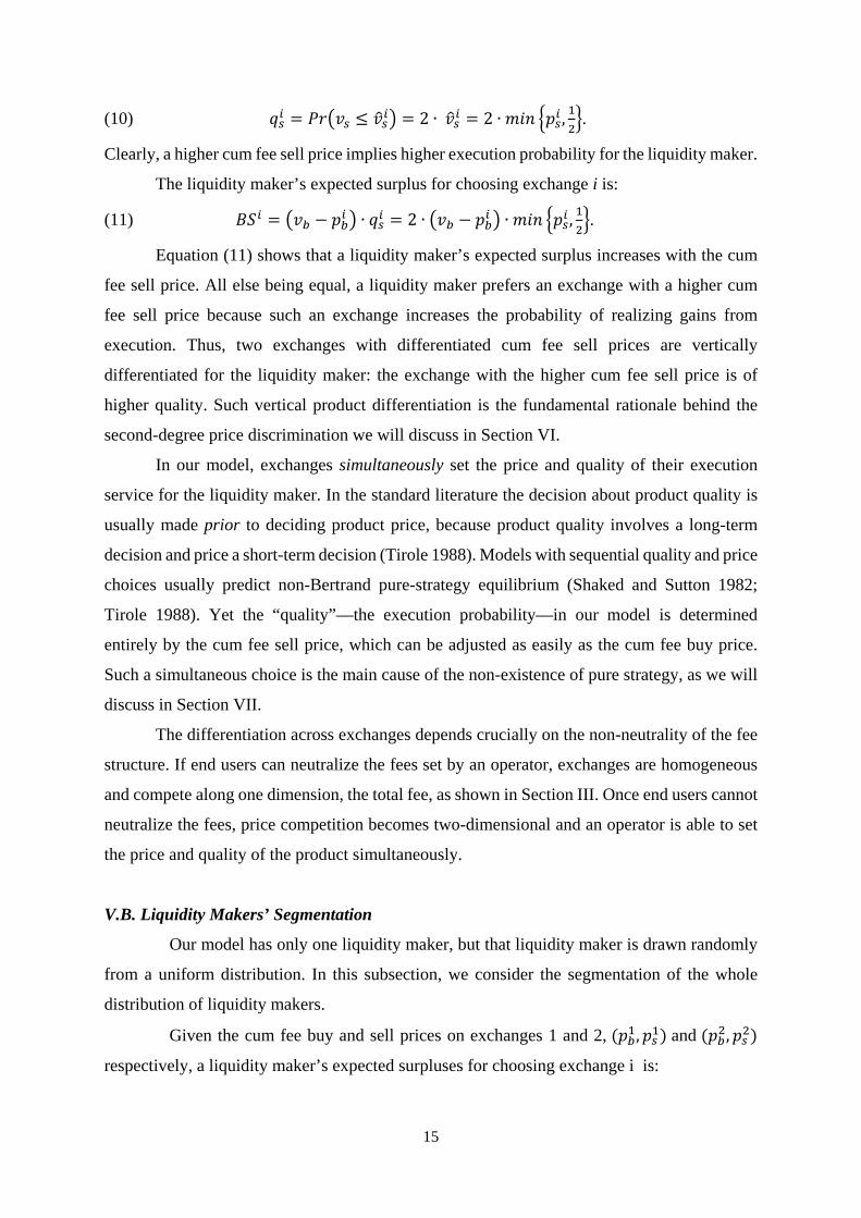
(10) 𝑞𝑞𝑠𝑠𝑖𝑖 = 𝑃𝑃𝑃𝑃�𝑣𝑣𝑠𝑠 ≤ 𝑣𝑣�𝑠𝑠𝑖𝑖� = 2 ∙ 𝑣𝑣�𝑠𝑠𝑖𝑖 = 2 ∙ 𝑚𝑚𝑖𝑖𝑛𝑛 �𝑝𝑝𝑠𝑠𝑖𝑖 ,12�.

Clearly, a higher cum fee sell price implies higher execution probability for the liquidity maker.

The liquidity maker’s expected surplus for choosing exchange i is:

(11) 𝐵𝐵𝐵𝐵𝑖𝑖 = �𝑣𝑣𝑏𝑏 − 𝑝𝑝𝑏𝑏𝑖𝑖 � ∙ 𝑞𝑞𝑠𝑠𝑖𝑖 = 2 ∙ �𝑣𝑣𝑏𝑏 − 𝑝𝑝𝑏𝑏𝑖𝑖 � ∙ 𝑚𝑚𝑖𝑖𝑛𝑛 �𝑝𝑝𝑠𝑠𝑖𝑖 ,12�.

Equation (11) shows that a liquidity maker’s expected surplus increases with the cum

fee sell price. All else being equal, a liquidity maker prefers an exchange with a higher cum

fee sell price because such an exchange increases the probability of realizing gains from

execution. Thus, two exchanges with differentiated cum fee sell prices are vertically

differentiated for the liquidity maker: the exchange with the higher cum fee sell price is of

higher quality. Such vertical product differentiation is the fundamental rationale behind the

second-degree price discrimination we will discuss in Section VI.

In our model, exchanges simultaneously set the price and quality of their execution

service for the liquidity maker. In the standard literature the decision about product quality is

usually made prior to deciding product price, because product quality involves a long-term

decision and price a short-term decision (Tirole 1988). Models with sequential quality and price

choices usually predict non-Bertrand pure-strategy equilibrium (Shaked and Sutton 1982;

Tirole 1988). Yet the “quality”—the execution probability—in our model is determined

entirely by the cum fee sell price, which can be adjusted as easily as the cum fee buy price.

Such a simultaneous choice is the main cause of the non-existence of pure strategy, as we will

discuss in Section VII.

The differentiation across exchanges depends crucially on the non-neutrality of the fee

structure. If end users can neutralize the fees set by an operator, exchanges are homogeneous

and compete along one dimension, the total fee, as shown in Section III. Once end users cannot

neutralize the fees, price competition becomes two-dimensional and an operator is able to set

the price and quality of the product simultaneously.

V.B. Liquidity Makers’ Segmentation

Our model has only one liquidity maker, but that liquidity maker is drawn randomly

from a uniform distribution. In this subsection, we consider the segmentation of the whole

distribution of liquidity makers.

Given the cum fee buy and sell prices on exchanges 1 and 2, (𝑝𝑝𝑏𝑏1,𝑝𝑝𝑠𝑠1) and (𝑝𝑝𝑏𝑏2,𝑝𝑝𝑠𝑠2)

respectively, a liquidity maker’s expected surpluses for choosing exchange i is:

16

(12) 𝐵𝐵𝐵𝐵𝑖𝑖 = �𝑣𝑣𝑏𝑏 − 𝑝𝑝𝑏𝑏𝑖𝑖 � ∙ 𝑞𝑞𝑠𝑠𝑖𝑖 = 2 ∙ �𝑣𝑣𝑏𝑏 − 𝑝𝑝𝑏𝑏i � ∙ 𝑝𝑝𝑠𝑠𝑖𝑖 , 𝑖𝑖 = 1,2

These equalities follow from 𝑣𝑣�𝑠𝑠𝑖𝑖 = 𝑝𝑝𝑠𝑠𝑖𝑖(𝑖𝑖 = 1,2), because neither exchange would set

𝑝𝑝𝑠𝑠𝑖𝑖 > 12 ): doing so would reduce its per-trade profit without increasing trading volume.

When 𝑝𝑝𝑠𝑠1 = 𝑝𝑝𝑠𝑠2, a liquidity maker’s surplus would be 𝐵𝐵𝐵𝐵1 ⋛ 𝐵𝐵𝐵𝐵2 if and only if 𝑝𝑝𝑏𝑏1 ⋚

𝑝𝑝𝑏𝑏2. Without loss of generality, suppose that 𝑝𝑝𝑠𝑠1 < 𝑝𝑝𝑠𝑠2, which implies that exchange 1 is of low

quality and exchange 2 is of high quality. The liquidity maker’s surpluses in each exchange are

shown in Figure III.

[Insert Figure III about here]

When 𝑝𝑝𝑏𝑏1 ≥ 𝑝𝑝𝑏𝑏2, as shown in Panel (a) of Figure III, 𝐵𝐵𝐵𝐵1 ≤ 𝐵𝐵𝐵𝐵2 for any 𝑣𝑣𝑏𝑏 ≥ 𝑝𝑝𝑏𝑏2. So

any liquidity maker chooses exchange 2, because exchange 2 offers higher execution

probability, along with a lower cum fee buy price.20

When 𝑝𝑝𝑏𝑏1 < 𝑝𝑝𝑏𝑏2, there is a unique intersection:

(13) 𝜑𝜑 ≡𝑝𝑝𝑏𝑏2 ∙ 𝑝𝑝𝑠𝑠2 − 𝑝𝑝𝑏𝑏1 ∙ 𝑝𝑝𝑠𝑠1

𝑝𝑝𝑠𝑠2 − 𝑝𝑝𝑠𝑠1

and 𝐵𝐵𝐵𝐵1 ⋚ 𝐵𝐵𝐵𝐵2 for any 𝑣𝑣𝑏𝑏 ⋛ 𝜑𝜑, as shown in Panel (b) of Figure III. Liquidity makers with a

valuation higher than 𝜑𝜑 choose high-quality exchange 2 and liquidity makers with a valuation

lower than 𝜑𝜑 choose low-quality exchange 1. Because we assume that 𝑣𝑣𝑏𝑏 is uniformly

distributed on [12

, 1], exchanges 1 and 2 co-exist when 12

< 𝜑𝜑 <1. All things being equal,

liquidity makers prefer the high-quality exchange. Yet liquidity makers are not uniformly

inclined to choose the higher execution probability. Those with larger gains from execution

care more about execution probability than those with smaller gains. This heterogeneity across

traders allows an exchange with higher cum fee buy and sell prices to coexist with an exchange

with lower cum fee buy and sell prices.

VI. MONOPOLY: PRICE DISCRIMINATION

In this section, we characterize a monopoly operator’s optimal choice of the number of

exchanges to offer as well as her choice of fee structure on each exchange. The purpose is to

explore the second-degree price discrimination facilitated by product differentiation.

20 In Figure I, we show that exchanges can have the same fees on one side but unequal fees on the other side. One reason for this phenomenon is that exchanges can also set their own criteria for traders to obtain a certain level of fees or rebates. Such criteria may lead to price discrimination within the same exchange, but our paper focuses on operators using multiple exchanges to conduct price discrimination.

17

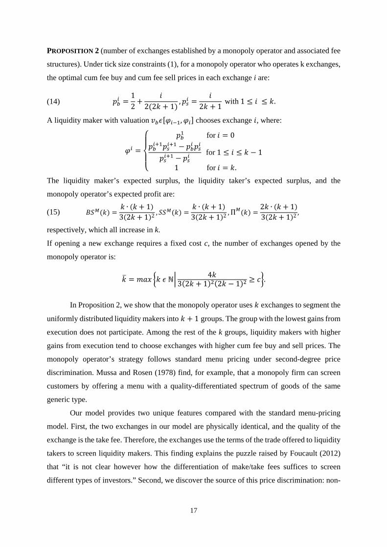
PROPOSITION 2 (number of exchanges established by a monopoly operator and associated fee

structures). Under tick size constraints (1), for a monopoly operator who operates k exchanges,

the optimal cum fee buy and cum fee sell prices in each exchange i are:

(14) 𝑝𝑝𝑏𝑏𝑖𝑖 =12

+𝑖𝑖

2(2𝑘𝑘 + 1),𝑝𝑝𝑠𝑠𝑖𝑖 =

𝑖𝑖2𝑘𝑘 + 1

with 1 ≤ 𝑖𝑖 ≤ 𝑘𝑘.

A liquidity maker with valuation 𝑣𝑣𝑏𝑏𝜖𝜖[𝜑𝜑𝑖𝑖−1,𝜑𝜑𝑖𝑖] chooses exchange 𝑖𝑖, where:

𝜑𝜑𝑖𝑖 =

⎩⎪⎨

⎪⎧ 𝑝𝑝𝑏𝑏1 for 𝑖𝑖 = 0𝑝𝑝𝑏𝑏𝑖𝑖+1𝑝𝑝𝑠𝑠𝑖𝑖+1 − 𝑝𝑝𝑏𝑏𝑖𝑖 𝑝𝑝𝑠𝑠𝑖𝑖

𝑝𝑝𝑠𝑠𝑖𝑖+1 − 𝑝𝑝𝑠𝑠𝑖𝑖 for 1 ≤ 𝑖𝑖 ≤ 𝑘𝑘 − 1

1 for 𝑖𝑖 = 𝑘𝑘.

The liquidity maker’s expected surplus, the liquidity taker’s expected surplus, and the

monopoly operator’s expected profit are:

(15) 𝐵𝐵𝐵𝐵𝑀𝑀(𝑘𝑘) =𝑘𝑘 ∙ (𝑘𝑘+ 1)3(2𝑘𝑘+ 1)2 , 𝐵𝐵𝐵𝐵𝑀𝑀(𝑘𝑘) =

𝑘𝑘 ∙ (𝑘𝑘+ 1)3(2𝑘𝑘+ 1)2 ,Π𝑀𝑀(𝑘𝑘) =

2𝑘𝑘 ∙ (𝑘𝑘+ 1)3(2𝑘𝑘+ 1)2 ,

respectively, which all increase in k.

If opening a new exchange requires a fixed cost c, the number of exchanges opened by the

monopoly operator is:

𝑘𝑘� = 𝑚𝑚𝑚𝑚𝑚𝑚 �𝑘𝑘 𝜖𝜖 ℕ� 4𝑘𝑘3(2𝑘𝑘 + 1)2(2𝑘𝑘 − 1)2 ≥ 𝑐𝑐�.

In Proposition 2, we show that the monopoly operator uses 𝑘𝑘 exchanges to segment the

uniformly distributed liquidity makers into 𝑘𝑘 + 1 groups. The group with the lowest gains from

execution does not participate. Among the rest of the k groups, liquidity makers with higher

gains from execution tend to choose exchanges with higher cum fee buy and sell prices. The

monopoly operator’s strategy follows standard menu pricing under second-degree price

discrimination. Mussa and Rosen (1978) find, for example, that a monopoly firm can screen

customers by offering a menu with a quality-differentiated spectrum of goods of the same

generic type.

Our model provides two unique features compared with the standard menu-pricing

model. First, the two exchanges in our model are physically identical, and the quality of the

exchange is the take fee. Therefore, the exchanges use the terms of the trade offered to liquidity

takers to screen liquidity makers. This finding explains the puzzle raised by Foucault (2012)

that “it is not clear however how the differentiation of make/take fees suffices to screen

different types of investors.” Second, we discover the source of this price discrimination: non-

18

neutrality led by the discrete price, because such price discrimination does not exist when

liquidity makers and liquidity takers can neutralize the fee breakdown.

We find that the monopoly operator’s profit increases with the number of exchanges,

but the marginal benefit of adding an exchange decreases with the number of existing

exchanges. Any fixed cost for establishing exchanges thus constrains the number of exchanges.

Interestingly, Equation (15) indicates that the liquidity maker’s and the liquidity taker’s

expected surpluses also increase with the number of exchanges. The welfare gain originates

from a higher participation rate: increasing the number of exchanges creates more cum fee

price levels within the tick. As 𝑘𝑘 goes to infinity, the lowest cum fee buy price across all

exchanges, 𝑘𝑘+12𝑘𝑘+1

, approaches 12, which indicates almost full participation by liquidity makers.

In our model, the creation of new cum fee price levels reduces the inefficiency created by

discrete tick size, which increases the expected trading gains for all parties.

Table I provides an example of second-degree price discrimination using make/take

fees. Column (1) shows that a monopoly that operates one exchange sets the cum fee buy price

at 𝑝𝑝𝑏𝑏𝑀𝑀 = 23 and the cum fee sell price at 𝑝𝑝𝑠𝑠𝑀𝑀 = 1

3. Liquidity makers with valuation in [2

3, 1] and

liquidity takers with valuation in [0, 13] participate in this exchange. The operator has a profit

of 427

. The second and third columns show that a monopoly can screen liquidity makers by

setting up two exchanges. The low-quality exchange sets the cum buy price at 𝑝𝑝𝑏𝑏1 = 35 and the

cum fee sell price at 𝑝𝑝𝑠𝑠1 = 15. The execution probability is 2

5 on the low-quality exchange, which

attracts liquidity makers with lower gains from execution (𝑣𝑣𝑏𝑏 ∈ [35

, 45] ). The high-quality

exchange sets the cum fee buy price at 𝑝𝑝𝑏𝑏2 = 710

and the cum fee sell price at 𝑝𝑝𝑠𝑠2 = 25. The

execution probability is 45 on the high-quality exchange, which attracts liquidity makers with

higher gains from execution (𝑣𝑣𝑏𝑏 ∈ [45

, 1]). This second-degree price discrimination increases

the monopoly’s profit from 427

to 425

. The expected surplus for both liquidity makers and

liquidity takers increases from 227

to 225

. The expected trading volume increases from 1227

to 1225

,

which provides a justification for the expected welfare gains for all parties.

[Insert Table I about here]

19

VII. COMPETITION: THE NON-EXISTENCE OF PURE-STRATEGY

EQUILIBRIUM

In this section, we consider the case of two competing operators, each of whom

establishes one exchange. In Section A, we establish the non-existence of the pure-strategy

equilibrium under tick size constraints. In Section B, we show the existence of symmetric

mixed-strategy equilibrium and that any mixed-strategy equilibrium leads to positive profit.

VII.A. No Pure-strategy Equilibrium

In Proposition 3, we show that tick size constraints destroy not only Bertrand

equilibrium but also any pure-strategy equilibrium.

PROPOSITION 3 (no pure-strategy equilibrium). Under tick size constraints (1), there exists no

pure-strategy equilibrium when two exchanges compete.

The detailed proof of this proposition is in the Appendix. Here we sketch the proof and

the corresponding intuitions. The non-existence of pure-strategy equilibrium with unequal

profits follows the intuition in the Bertrand game. The lower-profit exchange can increase its

expected profit by undercutting the higher-profit exchange’s cum fee buy price by 𝜀𝜀 and

mimicking its cum fee sell price.

Our model also does not have pure-strategy equilibrium entailing positive and equal

profits. If identical profits are led by identical price structures, one exchange can increase its

expected profit by undercutting its rival’s cum fee buy price by 𝜀𝜀 and mimicking its rival’s cum

fee sell price. The two-dimensional price competition also raises the possibility that two

exchanges have different price structures but the same total profits.21 Without loss of generality,

suppose that, initially, exchange 2 has higher quality than exchange 1 (𝑝𝑝𝑠𝑠2 > 𝑝𝑝𝑠𝑠1 = 𝛾𝛾). Figure

III shows that exchange 2 must have a higher cum fee buy price than exchange 1 (𝑝𝑝𝑏𝑏2 > 𝑝𝑝𝑏𝑏1 =

𝛿𝛿), and that liquidity makers with high valuations choose exchange 2 while liquidity makers

with low valuation choose exchange 1. A profitable deviation for exchange 2 is reducing the

cum fee sell price to 𝛾𝛾 and undercutting exchange 1’s cum fee buy price by setting its new cum

fee buy price to 𝛿𝛿 − 𝜀𝜀. This deviation allows exchange 2 to attract low-valuation liquidity

makers with infinitesimal profit concession. In addition, high-valuation liquidity makers still

choose exchange 2 because (i) they prefer (𝛿𝛿 − 𝜀𝜀, 𝛾𝛾) to (𝛿𝛿, 𝛾𝛾) and (ii) they choose to participate

21 Numerical examples of such cases are available from the author on request. For a general discussion of asymmetry networks, see Ambrus and Argenziano (2009).

20

because the cum fee buy price 𝛿𝛿 − 𝜀𝜀 is lower than their valuation. When 𝜀𝜀 is sufficiently small,

the expected profit from retaining high-valuation liquidity makers is greater than the

infinitesimal decrease in profit from low-valuation liquidity makers.22

Unlike the Bertrand game, no pure-strategy equilibrium exists here even if both

operators make zero profit. Two possible scenarios lead to the zero-profit outcome: (i) at least

one side of the market does not participate; or (ii) the cum fee buy and sell prices are equal.

Suppose that both exchanges have zero participation rates; in that case at least one of the two

operators can deviate profitably by facilitating some trades. Then we need only consider the

case in which one exchange sets the cum fee buy price equal to the cum fee sell price. Without

loss of generality, suppose that 𝑝𝑝𝑏𝑏1 = 𝑝𝑝𝑠𝑠1. The proof then involves two types of deviation.

First, we consider 𝑝𝑝𝑏𝑏1 = 𝑝𝑝𝑠𝑠1 ≥12. Then exchange 2 can have a profitable deviation by

setting 𝑝𝑝𝑏𝑏2 = 𝑝𝑝𝑏𝑏1 − 𝜇𝜇𝜀𝜀 , and 𝑝𝑝𝑠𝑠2 = 𝑝𝑝𝑠𝑠1 − 𝜀𝜀 with 𝜀𝜀 > 0 and 0 < 𝜇𝜇 < 1. When 𝑝𝑝𝑏𝑏1 = 𝑝𝑝𝑠𝑠1 > 12

,

exchange 2 reduces the cum fee sell price but not the execution probability, because any

liquidity taker accepts 𝑝𝑝𝑠𝑠2 = 12. A lower cum fee buy price then attracts liquidity makers with a

valuation above 𝑝𝑝𝑏𝑏2 to exchange 2, and exchange 2 makes a positive profit. When 𝑝𝑝𝑏𝑏1 = 𝑝𝑝𝑠𝑠1 = 12,

such a deviation reduces the execution probability, but also reduces the cum fee buy price,

which attracts liquidity makers with lower gains from execution; this is illustrated in Panel (a)

of Figure IV. Second, we consider 𝑝𝑝𝑏𝑏1 = 𝑝𝑝𝑠𝑠1 < 12. In this case the execution probability is less

than 1. Panel (b) of Figure IV shows that exchange 2 can have a profitable deviation by setting

𝑝𝑝𝑏𝑏2 = 𝑝𝑝𝑏𝑏1 + 𝜀𝜀 and 𝑝𝑝𝑠𝑠2 = 𝑝𝑝𝑠𝑠1 + 𝜇𝜇 ∙ 𝜀𝜀. Such a deviation increases the execution probability, and

also increases the cum fee buy price, which attracts liquidity makers with higher gains from

execution.

[Insert Figure IV about here]

Traditional price-quality games (Shaked and Sutton 1982; Tirole 1988) feature non-

Bertrand pure-strategy equilibrium. An important cause of the non-existence of pure-strategy

equilibrium in our model lies in the simultaneous choice of price and quality. If we allow the

operator to choose the take fee in the first stage and the make fee in the second stage, the model

generates standard non-Bertrand pure-strategy equilibrium (unreported for brevity). In most

22 Unlike the Bertrand game, the deviation to (𝛿𝛿 − 𝜀𝜀, 𝛾𝛾) does not attract all the original customers of exchanges 1 and 2. The participation probability of the liquidity taker decreases due to a drop in the cum fee sell price.

21

industries, it is natural to assume that the product quality decision is made prior to the product

price decision because price can often be adjusted faster than quality (Tirole 1988). Yet in our

model “quality,” in terms of execution probability, is determined purely by the cum fee sell

price. The cum fee sell price can be adjusted as easily as the cum fee buy price. Therefore, in

our setting, it is reasonable to consider simultaneous price and quality competition.

VII.B. Mixed-strategy Equilibrium

The non-existence of pure-strategy equilibrium further motivates us to investigate

symmetric mixed-strategy equilibria. It is a daunting task to find analytical solutions for all

possible mixed-strategy equilibria. Nevertheless, we are able to demonstrate the existence of a

symmetric mixed-strategy equilibrium and prove that it always entails positive profit.

PROPOSITION 4 (mixed-strategy equilibrium). Under tick size constraints (1):

(i) symmetric mixed-strategy equilibrium exists;

(ii) in equilibrium, both exchanges earn strictly positive profits.

The proof of Proposition 4 shows that our game satisfies conditions specified in

Theorem 6* of Dasgupta and Maskin (1986), which studies the mixed-strategy equilibrium

existence problem in a discontinuous game.

Varian (1980) states that the mixed-strategy equilibrium justifies the spatial price

dispersion (different prices at the same time) and temporal price dispersion (price change over

time). From this perspective, our paper provides the first theoretical justification for diverse

fee structures across exchanges and their frequent changes. As indicated by an SEC statement,

“these exchanges compete vigorously on price which leads to some rather complicated fee

schedule that can change from month to month, making it a near full-time job to keep track of

them all.” 23 The driver of our mixed-strategy equilibrium, however, differs significantly from

those in canonical one-dimensional mixed-strategy equilibrium. In the literature, one-

dimensional mixed-strategy equilibrium generally involves frictions that prevent customers

from finding the best price (Rosenthal 1980; Varian 1980; Burdett and Judd 1983), or cost to

firms to transmit their prices (Butters 1977; Baye and Morgan 2001). For example, Rosenthal

(1980) assumes loyal customers, while Varian (1980) assumes uninformed customers who are

not aware of better prices. The incentive to exploit loyal or uninformed customers prevents

23 See Richard Holley, SEC Trading and Division, Statement in Panel Discussion at SEC Equality Market Structure Advisory Committee Meeting on October 27, 2015, available at https://www.sec.gov/news/otherwebcasts/2015/equity-market-structure-advisory-committee-102715.shtml.

22

firms from undercutting each other toward the marginal cost. In our model, the liquidity maker

and liquidity taker fully optimize their choices, are fully aware of the fees, and exchanges do

not feature any costs to transmit make/take fees to traders. The driving force behind the mixed-

strategy equilibrium is two-dimensional price competition. When price competition is one-

dimensional, all customers prefer a lower price even if their valuations are heterogeneous. No

such consensus exists if price competition is two-dimensional. As Figure 3 demonstrates,

liquidity makers choose different fee structures based on gains from execution.

The existence of strictly positive profit in mixed-strategy equilibrium rationalizes the

entries of new exchanges and market fragmentation. This result arises from the two-sided

feature of the markets caused by tick size regulation. When the tick size is zero, as shown in

Section III, the markets are one-sided. Hence, competition between two exchanges can drive

their profits to zero (Colliard and Foucault 2012), which implies that any positive cost involved

in establishing a new stock exchange would deter entry. In reality, however, we continue to

witness “the formation of new exchanges to experiment different price structures.”24 When the

tick size is positive, the markets become two-sided. Competition between exchanges does not

lead them to earn zero profit, which encourages the entry of new exchanges. Regulators are

often concerned that the entry of new stock exchanges will generate greater market

fragmentation (O’Hara and Ye 2011), but there is only limited understanding of why the market

becomes increasingly fragmented. We show that one driving force behind fragmentation is the

existing tick size regulation.

VIII. ROBUSTNESS CHECK AND EXTENSIONS

In this section, we relax two assumptions made in Sections IV–VII. In Section VIII.A.

we allow trades to occur on more price grids by reducing the tick size while keeping traders’

valuations constant. In Section B, we relax the assumption of duopoly operators, and allow

each operator to choose the number of exchanges. These extensions produce qualitatively

similar results to those reported in Sections IV–VII.

VIII.A. Multiple Ticks

In previous sections we compare market outcomes when the tick size is equal to zero

with those that obtain when the tick size is equal to 1. All else being equal, in this subsection,

24 Holley, fn 23.

23

we consider the case in which the tick size is equal to 1𝑁𝑁

, where N is a natural number greater

than 1. As a liquidity maker has more price grids from which to choose, exchanges cannot

mandate unique cum fee buy and sell prices by setting make and take fees. Predictions under

this relaxed setting, however, are qualitatively similar to those under N = 1. As long as the tick

size is not zero, exchanges can use make and take fees to create sub-tick prices that cannot be

neutralized by end users, which facilitates second-degree price discrimination and destroys

pure-strategy equilibrium.

We start from the simplest case, in which a monopoly opens one exchange. We solve

the problem backwards by first considering the limit-order price proposed by the liquidity

maker.

PROPOSITION 5 (the limit-order price proposed by the liquidity maker). Under tick size

constraints (1′)

i) The liquidity maker submits no limit order when 𝑣𝑣𝑏𝑏 < 𝑓𝑓𝑚𝑚 + ⌈𝑁𝑁∙𝑓𝑓𝑡𝑡⌉𝑁𝑁

, and a liquidity

maker submits a limit order at price 𝑃𝑃 = 𝑛𝑛(𝑣𝑣𝑏𝑏,𝑓𝑓𝑚𝑚,𝑓𝑓𝑡𝑡)𝑁𝑁

otherwise. Here

𝑛𝑛(𝑣𝑣𝑏𝑏,𝑓𝑓𝑚𝑚, 𝑓𝑓𝑡𝑡) = �𝑁𝑁 ∙ (𝑣𝑣𝑏𝑏 − 𝑓𝑓𝑚𝑚 + 𝑓𝑓𝑡𝑡) + 1

2� ,

where ⌈𝑚𝑚⌉ and ⌊𝑚𝑚⌋ denote the ceiling and floor functions, respectively.

ii) Compared with fee structure (𝑓𝑓𝑚𝑚,𝑓𝑓𝑡𝑡), fee structure (𝑓𝑓𝑚𝑚 + 𝑘𝑘𝑁𝑁

, 𝑓𝑓𝑡𝑡 −𝑘𝑘𝑁𝑁

), 𝑘𝑘 ∈ 𝑍𝑍 shifts

the limit-order price proposed by the liquidity maker by -k ticks, but leads to the

same cum fee buy and sell prices as those that occur under fee structure (𝑓𝑓𝑚𝑚,𝑓𝑓𝑡𝑡).

Proposition 5 shows that, for a given total fee, if the exchange increases its make fee

by, say, one tick, then a liquidity maker can neutralize the effect of this increase by proposing

a limit-order price that is one tick lower, leaving the cum fee buy and sell prices unchanged.

Therefore, Part (i) of Proposition 1 is a limiting case of Proposition 5: when the tick size is

zero, a liquidity maker is able to neutralize any fee breakdowns.

Proposition 5 also demonstrates that the limit-order price is a non-decreasing step

function of the liquidity maker’s valuation: a liquidity maker with higher gains from execution

tends to propose a higher limit-order price to increase the probability of execution. Unlike

continuous pricing, the limit-order price does not strictly increase in 𝑣𝑣𝑏𝑏, as 𝑛𝑛(𝑣𝑣𝑏𝑏,𝑓𝑓𝑚𝑚,𝑓𝑓𝑡𝑡)𝑁𝑁

involves

a floor function of 𝑣𝑣𝑏𝑏 . When pricing is discrete, the unconstrained limit-order price that a

24

liquidity maker would propose might not coincide with any of the price grids, which results in

the same limit-order price proposed by liquidity makers with heterogeneous valuations.

The second-degree price discrimination under multiple ticks involves screening

liquidity makers who have heterogeneous valuations but quote the same price. Obtaining the

analytical solution for the optimal fee structure is a complex process, because the nominal price

proposed by the liquidity maker 𝑛𝑛(𝑣𝑣𝑏𝑏,𝑓𝑓𝑚𝑚, 𝑓𝑓𝑡𝑡) involves a floor function of 𝑓𝑓𝑚𝑚 and 𝑓𝑓𝑡𝑡. For the

case of a monopoly opening one exchange, we are able to obtain the optimal fee structure as a

function of N, and we present the results in Appendix B. We are not able to obtain a closed-

form solution for the optimal make and take fees as a function of N when the operator

establishes two exchanges. Therefore, we conduct a numerical search and present the results

for N = 2, 4, and 8 as examples in Table II.25

Table II shows that the N = 2 case is identical to the N = 1 case, as the tick size is still

large enough for the monopoly operator to mandate unique cum fee buy and sell prices by

setting make and take fees. The N = 4 and N = 8 cases illustrate two interesting features.

[Insert Table II about here]

First, the monopoly obtains strictly higher profits by establishing two vertically

differentiated exchanges than by establishing one exchange. For example, for N = 4, the low-

quality exchange sets the take fee at −0.0340 and the high-quality exchange sets the take fee at

−0.1595. The exchange with the lower take fee is of higher quality because a liquidity maker

always chooses the exchange with the lower take fee if both exchanges set the same make fee.26

The second-degree price discrimination involves charging a low make fee (0.4095) for the low-

quality exchange and a high make fee (0.5840) for the high-quality exchange. The operator

increases her total profit from 0.1406 to 0.1445.27

Second, liquidity makers rotate between the low-quality and the high-quality exchange

as their valuation increases. For example, under tick size 14, a liquidity maker with valuation

25 Our Internet Appendix provides C++ code for the simulations. We restrict the level of the take fee to [− 1

𝑁𝑁, 0]

in the simulation, as the equivalence of fee structures (𝑓𝑓𝑚𝑚, 𝑓𝑓𝑡𝑡) and (𝑓𝑓𝑚𝑚 + 𝑘𝑘𝑁𝑁

, 𝑓𝑓𝑡𝑡 −𝑘𝑘𝑁𝑁

), 𝑘𝑘 ∈ 𝑍𝑍 suggested by Proposition 5. 26 To see this, consider two exchanges with different take fees but charging the same make fee. Suppose that the optimal limit-order price for the liquidity maker is 𝑃𝑃∗ on the high take-fee exchange. If the liquidity maker proposes the same 𝑃𝑃∗ on the low take-fee exchange, her gain from execution remains the same but the lower take fee increases her execution probability. Therefore, she would achieve a higher expected surplus by proposing the same 𝑃𝑃∗ on the lower take-fee exchange. The optimal price for the liquidity maker on the low-fee exchange may be different from 𝑃𝑃∗on the high-take fee exchange, but a different optimal price implies that the liquidity maker can achieve even higher expected surplus than proposing 𝑃𝑃∗ in the low take-fee exchange. 27 0.1445 is the sum of the profits from the low-quality exchange and the high-quality exchange.

25

𝑣𝑣𝑏𝑏 ∈ [0.5000,0.6313] proposes a limit order at 𝑃𝑃 = 0 on the low-quality exchange. A

liquidity maker with valuation 𝑣𝑣𝑏𝑏 ∈ [0.6313, 0.7562] chooses the high-quality exchange, and

proposes the same price 𝑃𝑃 = 0 . Interestingly, a further increase in valuation to 𝑣𝑣𝑏𝑏 ∈

[0.7562, 1.000] leads a liquidity maker to switch back to the low-quality exchange with an

increased limit-order price of 𝑃𝑃 = 14. In fact, column (9) in Table II reveals that a liquidity

maker with the lowest valuation 𝑣𝑣𝑏𝑏∈[0.5000, 0.6501] chooses the high-quality exchange and

proposes a limit order at price 𝑃𝑃 = 0.

The rotation of the exchange choice seems to suggest horizontal differentiation of

exchanges. Yet exchanges in our model are only vertically differentiated: all else being equal,

all liquidity makers prefer an exchange with a lower take fee. Exchange rotation is driven by

the definitions of the high valuation and low valuation types in our model. Unlike the usual

models of vertical differentiation, the high and low types in our game are defined on each price

grid. Table II shows that, at the same proposed limit-order price, liquidity makers who choose

the high-quality exchange have higher valuation than those who choose the low-quality

exchange. For example, for N = 8, liquidity makers who propose 𝑃𝑃 = 18 on the low-quality

exchange have valuations in [0.6501, 0.7334], whereas liquidity makers who propose 𝑃𝑃 = 18 on

the high-quality exchange have valuations in [0.7334, 0.9164]. Yet a further increase in

valuation beyond 0.9164 makes a liquidity maker propose a price of 14 on the low-quality

exchange. The nature of such second-degree price discrimination is to screen liquidity makers

with relatively high and low valuations on the same price grid. Therefore, the price

discrimination with multiple ticks serves as an extension of our baseline model with only one

tick, in which all liquidity makers have to quote the same price.

VIII.B. Multiple Operators Each Choosing the Number of Exchanges

In this subsection, we allow multiple operators to participate in the game, and each

operator can choose the number of exchanges to offer. Still, no pure-strategy equilibrium exists

as long as pricing is discrete.

PROPOSITION 6. Under tick size constraints (1′), no pure-strategy equilibrium exists when the

number of operators is greater than 1.

Allowing an operator to choose the number of exchanges introduces a new type of

profitable deviation: increasing the number of exchanges. Proposition 6 holds for any discrete

26

tick size. Here we offer an intuitive explanation based on a tick size of 1. Suppose the number

of exchanges with positive profits is H. We can always find an operator who does not own all

these H exchanges. The operator can increase her profits by establishing H new exchanges,

each of which undercuts the cum fee buy prices of the existing H exchanges by 𝜀𝜀, and sets the

same cum fee sell prices. Such a deviation allows the operator to capture the entire market. In

reality, opening an additional exchange to compete with rivals is certainly more aggressive

than changing fees on an existing exchange. Yet we find evidence consistent with this strategy.

The exchange industry starts from the maker/taker model that offers rebates to liquidity makers

while charging takers. On April 1, 2009, the Boston Stock Exchange became the first exchange

to charge liquidity makers and subsidize liquidity takers. This inverted fee structure was

subsequently adopted by Direct Edge’s new exchange EDGA, and BATS soon followed by

establishing the BATS Y. 28 Among the three current major operators—NASDAQ OMX,

Intercontinental Exchange (ICE), and BATS Global Markets)—only the ICE has no exchange

with an inverted fee structure. However, in a recent panel discussion held by the SEC, the

president of the NYSE admitted that, facing pressure from competitors, the NYSE is

considering establishing an exchange with an inverted fee structure. 29

Now consider the case in which all exchanges make zero profit. An exchange has zero

profit if (i) no trader participates in that exchange or (ii) the cum fee buy price equals the cum

fee sell price. For exchanges with a positive participation rate, we can find the one with the

lowest cum fee price, 𝑝𝑝𝑚𝑚𝑖𝑖𝑛𝑛. The operator can find a profitable deviation by establishing a new

exchange using the same deviating strategy depicted in the proof of Proposition 3. If 𝑝𝑝𝑚𝑚𝑖𝑖𝑛𝑛 < 12,

the new exchange can choose 𝑝𝑝𝑏𝑏𝑛𝑛𝑛𝑛𝑛𝑛 = 𝑝𝑝𝑚𝑚𝑖𝑖𝑛𝑛 + 𝜀𝜀 and 𝑝𝑝𝑠𝑠𝑛𝑛𝑛𝑛𝑛𝑛 = 𝑝𝑝𝑚𝑚𝑖𝑖𝑛𝑛 + 𝜇𝜇𝜀𝜀 (0 < 𝜇𝜇 < 1) . This

pricing structure increases both the cum fee buy price and execution probability, thus attracting

liquidity makers with high gains from execution. If 𝑝𝑝𝑚𝑚𝑖𝑖𝑛𝑛 ≥ 12, the new exchange can choose

𝑝𝑝𝑏𝑏𝑛𝑛𝑛𝑛𝑛𝑛 = 𝑝𝑝𝑚𝑚𝑖𝑖𝑛𝑛 − 𝜇𝜇𝜀𝜀 and 𝑝𝑝𝑠𝑠𝑛𝑛𝑛𝑛𝑛𝑛 = 𝑝𝑝𝑚𝑚𝑖𝑖𝑛𝑛 − 𝜀𝜀 and attracts liquidity makers with low gains from

execution.

IX. DISCUSSION AND POLICY IMPLICATIONS

In this section, we discuss the policy implications of our results. In Section IX.A., we

28 BATS established BATS Y before its acquisition of Direct Edge. 29 See Thomas Farley, President of the NYSE, panel discussion during the Equity Market Structure Advisory Committee Meeting at SEC on October 27, 2015, available at: https://www.sec.gov/news/otherwebcasts/2015/equity-market-structure-advisory-committee-102715.shtml.

27

discuss recent policy debates on the maker/taker pricing model. In Section IX.B., we discuss

the new insights our paper provides on the proliferation of new order types and alternative

trading systems such as dark pools.

IX.A. Policy Debates on the Maker/Taker Pricing Model

Recently, the holding company of the NYSE, the ICE, proposed eliminating the

maker/taker pricing model.30 Two replacement fee structures were proposed: (i) reducing take

fees after eliminating rebates31; and (ii) distributing the total fee equally between liquidity

makers and liquidity takers32. BATS, on the other hand, aggressively opposes banning the

maker/taker pricing structure. 33 Proposition 7 predicts market outcomes under these two

proposed fee structures.

PROPOSITION 7. Under tick size constraints (1′), eliminating rebates, thereby charging only

one side, or splitting the total fee equally between a liquidity maker and a liquidity taker:

(i) leads competing operators to make zero profit;

(ii) discourages operators from opening more than one exchange.34

First, consider the policy proposal to remove rebates to liquidity makers and to charge

only liquidity takers. Any liquidity maker then chooses the exchange with the lowest take fee,

because it offers the highest quality at the same zero make fee. Our model also allows us to

evaluate the consequence of charging liquidity makers only. In this case, competing exchanges

are of the same quality and the liquidity maker chooses the exchange with the lowest price

(make fee). Charging only one side changes the two-sided price competition to one-sided price

competition, which leads competing operators to undercut each other toward zero make and

take fees. Also, no operators have incentives to establish multiple exchanges, because the

liquidity maker always chooses the exchange with the lowest fee.

The proposal to split the total fee equally between a liquidity maker and a liquidity taker

also changes two-sided price competition to one-sided price competition. When such a

restriction is imposed, a high-quality (low take fee) exchange must also charge a low price (or

30 Sprecher, fn 8. 31 Sprecher, fn 8. 32 See Matt Lyons, Senior V.P. & Global Trading Manager of the Capital Group, Panel Discussion at SEC on October 27, 2015, available at: https://www.sec.gov/news/otherwebcasts/2015/equity-market-structure-advisory-committee-102715.shtml. 33 Ratterman, fn 9. 34 When 𝑁𝑁 = 1, charging one side only or splitting the total fee equally results in no trade (Lemma 1). Thus, all exchanges make zero profit. The proposition holds trivially.

28

low make fee), which destroys the exchange’s ability to balance price and quality with respect

to the liquidity maker. The liquidity maker thus chooses the exchange with the lowest total fee,

which in turn results in competing operators undercutting each other toward a zero total fee,

and no operators having an incentive to establish multiple exchanges.

Proposition 7 provides a possible rationale for the differing stances of operators on the

policy debate over fee schedules. A major concern of traditional stock exchanges such as the

NYSE is the loss of market share to new market entrants such as BATS. Under two-sided price

competition, the proof of Proposition 3 demonstrates that no operator can prevent its rivals

from making strictly positive profits without losing money itself. One-dimensional price

competition, however, can drive profits toward zero. This provides a plausible explanation of

why BATS aggressively opposes one-dimensional price competition, as its major source of

revenue comes from make/take fees. The NYSE, however, obtains revenue from stock listings

as well as fees; this additional revenue could help it to survive short-run zero profit from

make/take fees. To be sure, the opposing positions taken by the NYSE and BATS in the policy

debate can be driven by other considerations, but the extant literature has yet to explain their

divergence of opinion.35

Surprisingly, having competition to drive exchange profit to zero may not necessarily

improve social welfare under a discrete tick size. As demonstrated in Lemma 1, suppose that

the tick size equals 1 and the liquidity maker’s valuation is 𝑣𝑣𝑏𝑏 ∈ [12

, 1] while the liquidity

taker’s valuation is 𝑣𝑣𝑠𝑠 ∈ [0, 12]. Charging one side while subsidizing the other creates a new

price level within a tick that can facilitate trades, while charging one side or equal splitting

results in no trades occurring, and consequently a loss of social welfare. By contrast, suppose

that the tick size equals 12, and the liquidity maker’s and liquidity taker’s valuations stay the

same as in the previous case but they are now separated by the price grid P = 12. In this case,

charging no fees to either side facilitates all trading on the price grid 12, which improves social

welfare. In the real world, the liquidity maker’s and liquidity taker’s valuations can either fall

within a tick or be separated by a price grid. Under a discrete tick size, the overall effect of

having zero make and take fees on social welfare is mixed.

35 For example, the NYSE argues that brokers tend to route orders to exchanges with the highest rebates, because brokers are not required to pass on the rebates to customers. Yet it is puzzling why the NYSE does not simply match the rebates offered by BATS as a competing device, and instead calls on regulators to ban the rebates. BATS argues that the NYSE’s proposal to ban the rebate is anticompetitive, but it is not clear why price competition in a one-dimensional configuration is less competitive than in a two-dimensional configuration.

29

IX.B. Implications for the Proliferation of Order Types and Dark pools

The nature of the fee game is that the operator proposes sub-tick price increments within

a given tick. Such an interpretation also sheds light on the proliferation of new order types and

dark pools. SEC Rule 612(c) imposes the tick size on displayed orders, but operators can create

sub-penny prices using hidden order types or by creating trading systems in which the quotes

are hidden. For example, midpoint peg orders have a nominal price at the midpoint, while the

midpoint dark pool matches buyers and sellers using the midpoint of the national best bid and

offer prices. The pricing of these two mechanisms is similar to a fee structure of

(𝑓𝑓𝑚𝑚 = 0.5,𝑓𝑓𝑡𝑡 = −0.5) in our model. This fee structure facilitates trading between any liquidity

maker and any liquidity taker with valuations specified in our model. In a competitive

environment, however, the fee structure (𝑓𝑓𝑚𝑚 = 0.5,𝑓𝑓𝑡𝑡 = −0.5) cannot preempt the entry of

other fee structures, other order types, or the dark pools implied by the fee structure, as is

posited in Proposition 3.

More importantly, new order types and dark pools are run by for-profit institutions that

charge service fees, so the implied fee structures are different from (𝑓𝑓𝑚𝑚 = 0.5,𝑓𝑓𝑡𝑡 = −0.5). We

are aware that new order types and dark pools can serve other purposes, such as hiding

information. Nevertheless, our model provides one explanation for the proliferation of new

order types and dark pools. This intuition is consistent with the empirical evidence reported by

Kwan, Masulis, and McInish (2015), that the market share of a dark pool increases with the

relative tick size (a one-cent tick size divided by the stock price). Also, we provide one

plausible explanation why new order types and dark pools do not drive public exchanges and

regular limit and market orders out of business, despite their ability to provide transaction costs

within the tick.

X. CONCLUSION

In this paper, we examine make/take fee competition between stock exchanges. When

traders can quote a continuous price, the breakdown of the make/take fees is neutralized and

order flow consolidates to the exchange with the lowest total fee. Under tick size constraints,

fee breakdowns are no longer neutral, and two-sided competition over make and take fees leads

to the proliferation of stock exchanges offering almost identical services but charging dispersed

fees. We first show that the two-sidedness of such a market allows operators to establish

multiple, intrinsically identical, exchanges with heterogeneous fee structures for the purpose

of second-degree price discrimination. Second, we demonstrate the non-existence of pure-

30

strategy equilibrium in the fee game under tick size constraints, which leads to fee diversity

and frequent fluctuations. Mixed-strategy equilibrium entails positive profits for all competing

operators, which encourages the entry of exchanges with new fee structures.

This understanding of the nature of make/take fee competition helps in the evaluation

of a recent proposal to ban maker/taker pricing model. There are three arguments for banning

the make/take fee pricing model: fairness, complexity, and agency issues. The fairness

argument claims that fees lead to wealth transfer from one side of the market to the other. We

show, however, that in the presence of tick size constraints the fees imposed by the exchanges

can improve welfare by creating sub-tick transaction prices. The second argument for banning

the fee cites its complexity and frequent fluctuations. Since the literature provides limited

economic rationale for this complexity, Dolgopolov (2014) and Lewis (2014) conjecture that

such complexity may serve fraudulent practices to disproportionately benefit certain market

participants (SEC 2015). However, the mixed-strategy equilibrium in the model provides an

alternative interpretation of this complexity. The final argument for banning the fee involves

agency concerns. Battalio, Corwin, and Jennings (2015) find that broker/dealers have a strong

incentive to route customers’ limit orders to the market offering the highest rebate, because

brokers/dealers are permitted to keep such rebates. This conflict of interest leads to two policy

proposals: (i) passing the rebate back to customers; and (ii) eliminating the fees (Angel, Harris,

and Spatt 2010, 2013). This paper reveals economic forces that favor the first solution. Passing

the rebate back to customers is a direct solution to the agency issue, while eliminating the fees

might hinder the would-be efficiency of trading within the tick size. Finally, our model predicts

that charging one side or splitting fees equally would drive make and take fees toward zero,

but the welfare effects of these proposals are mixed under tick size constraints.

We also show that make/take fees are responses from competing exchanges seeking to

bypass the existing tick size regulations. 36 This result questions the rationale of a recent

initiative to increase the tick size for small stocks to five cents. Encouraged by the 2012 JOBS

Act, the SEC plans to implement a pilot program to increase the tick size on May 6, 2016.37

The motivation for increasing the tick size is that it may increase market-making profits,

support sell-side equity research, and, eventually, increase the number of IPOs (Weild, Kim,

and Newport 2012). We show, however, that exchanges can use fee structures to create cum

36 For studies on the tick size, see Kandel and Marx (1997), Kalay and Anshuman (1998), Buti et al. (2014), O’Hara, Saar, and Zhong (2015), and Yao and Ye (2015), among others. 37 See SEC press release “SEC Approves Pilot to Assess Tick Size Impact for Smaller Companies” on May 6, 2015, available at http://www.sec.gov/news/pressrelease/2015-82.html.

31

fee prices that fall within the tick. An increase in the tick size will potentially create more room

for multiple exchanges to co-exist and lead to a more fragmented market.

Our model is based on the stock exchange industry, but it reveals two economic

mechanisms that can potentially be extended to other industries. First, non-neutrality in our

paper stems from the tick size regulation in the exchange industry, but we believe this economic

insight applies to other market frictions that also generate non-neutrality. For example, non-

surcharge provisions in credit card contracts discourage merchants from charging differentiated

prices for payments using different credit cards. The similarity between credit cards and

make/take fees resides in market designs that prevent the two user groups from neutralizing the

breakdown of the fees. Cards with high rebates to customers generally have lower acceptance

rates because they usually charge a high fee to merchants. Suppose that merchants can impose

surcharges on transactions to recover the fees they are charged. Credit card issuers would

compete over the sum of charges to both merchants and card-holders, which could reduce the

variety of credit cards. It would be interesting to explore whether gradual removal of non-

surcharge provision would reduce the variety of credit cards.38 Second, the non-existence of a

pure-strategy equilibrium in our model is driven by the simultaneous choice of price and quality.

In our paper, quality refers to another price (execution probability implied by the cum fee price

for the liquidity taker), but the predictability of the model should hold if quality is a product

feature that can be easily adjusted. Such a feature may be hard to find in manufacturing, but

we believe it may exist in financial or service-oriented industries. Thus, we hope that this paper

proves fruitful in generating further useful research in the competition between financial

products.

UNIVERSITY OF LOUISVILLE

UNIVERSITY OF WARWICK

UNIVERSITY OF ILLINOIS AT URBANA-CHAMPAIGN

38 Since January 27, 2013, 40 U.S. states have allowed merchants to add a surcharge to purchases paid with a Visa or MasterCard. However, the competition between credit cards is still two sided. First, this settlement does not cover all states. Second, this settlement does not cover all cards. A merchant that accepts American Express cannot surcharge Visa and MasterCard credit cards. Most importantly, merchants are not allowed to discriminate or surcharge based on the involved payment card issuer (i.e. national bank, state bank, credit union, etc.), or whether the card is a rewards card or a non-rewards card.

32

APPENDIX A: PROOFS

Proof of PROPOSITION 1

Part (i) follows from Equation (2), which implies that for any 𝑣𝑣𝑏𝑏 ≥ 𝑇𝑇𝑖𝑖, the maximal

surplus for a buyer with valuation 𝑣𝑣𝑏𝑏 to submit a limit order to exchange (hereafter, EX) i is

𝐵𝐵𝐵𝐵𝑖𝑖∗(𝑣𝑣𝑏𝑏) = �𝑣𝑣𝑏𝑏 − 𝑃𝑃𝑖𝑖∗(𝑣𝑣𝑏𝑏) − 𝑓𝑓𝑚𝑚𝑖𝑖 � ∙ Prob �𝑣𝑣𝑠𝑠 ≤ 𝑚𝑚𝑖𝑖𝑛𝑛 �𝑃𝑃𝑖𝑖∗(𝑣𝑣𝑏𝑏) − 𝑓𝑓𝑡𝑡𝑖𝑖 ,12��

= �𝑣𝑣𝑏𝑏 − 𝑇𝑇𝑖𝑖� ∙ 𝑚𝑚𝑖𝑖𝑛𝑛 �𝑣𝑣𝑏𝑏 − 𝑇𝑇𝑖𝑖

2,12�

= �𝑣𝑣𝑏𝑏−𝑇𝑇𝑖𝑖�2

2 (because 𝑣𝑣𝑏𝑏 − 𝑇𝑇𝑖𝑖 ≤ 1 for any 𝑇𝑇𝑖𝑖 ≥ 0),

which depends only on total fee 𝑇𝑇𝑖𝑖. Consequently, the liquidity maker chooses the EX with the

lowest total fee. Since the liquidity taker follows the liquidity maker’s choice of EX, she also

chooses the EX with the lowest total fee.

For any given 𝑣𝑣𝑏𝑏, the EX with the lowest total fee earns a profit

𝛱𝛱�𝑇𝑇𝑖𝑖 , 𝑣𝑣𝑏𝑏� = �𝑇𝑇𝑖𝑖 ∙ Prob �𝑣𝑣𝑠𝑠 ≤ min �𝑃𝑃𝑖𝑖∗(𝑣𝑣𝑏𝑏) − 𝑓𝑓𝑡𝑡𝑖𝑖 ,

12�� 𝑖𝑖𝑓𝑓 𝑣𝑣𝑏𝑏 ≥ 𝑇𝑇𝑖𝑖

0 𝑖𝑖𝑓𝑓 𝑣𝑣𝑏𝑏 < 𝑇𝑇𝑖𝑖.

Accordingly, its total expected profit is given by

𝛱𝛱𝑐𝑐𝑐𝑐𝑛𝑛𝑡𝑡 = � 2 ∙ 𝛱𝛱�𝑇𝑇𝑖𝑖 , 𝑣𝑣𝑏𝑏� 𝑑𝑑𝑣𝑣𝑏𝑏𝑣𝑣𝑏𝑏≥𝑇𝑇𝑖𝑖

= 2𝑇𝑇𝑖𝑖 ∙ � Prob �𝑣𝑣𝑠𝑠 ≤ min �𝑃𝑃𝑖𝑖∗(𝑣𝑣𝑏𝑏) − 𝑓𝑓𝑡𝑡𝑖𝑖 ,12�� 𝑑𝑑𝑣𝑣𝑏𝑏

1

max�𝑇𝑇𝑖𝑖, 12�

= 2𝑇𝑇𝑖𝑖 ∙ � Prob�𝑣𝑣𝑠𝑠 ≤𝑣𝑣𝑏𝑏 − 𝑇𝑇𝑖𝑖

2�𝑑𝑑𝑣𝑣𝑏𝑏

1

max�𝑇𝑇𝑖𝑖, 12�

= 2𝑇𝑇𝑖𝑖 ∙ � (𝑣𝑣𝑏𝑏 − 𝑇𝑇𝑖𝑖)𝑑𝑑𝑣𝑣𝑏𝑏1

max�𝑇𝑇𝑖𝑖, 12�

which is a function of 𝑇𝑇𝑖𝑖, and does not depend on how 𝑇𝑇𝑖𝑖 is decomposed into 𝑓𝑓𝑚𝑚𝑖𝑖 and 𝑓𝑓𝑡𝑡𝑖𝑖. EXs

whose total fees are not the lowest earn zero profits.

Thus for all three types of players, only the total fee matters.

Parts (ii) and (iii) follow directly from part (i). Since all traders go to the EX with the

lowest total fee, no operator can increase its profit by establishing multiple exchanges with

heterogeneous total fee. When multiple operators compete, they undercut each other to zero

total fee and earn zero profits.

33

To solve for optimal monopoly pricing, note that a monopoly operator does not have

any incentive to open multiple EXs, because any liquidity maker chooses the EX with the

lowest total fee. So using the formula for 𝛱𝛱𝑐𝑐𝑐𝑐𝑛𝑛𝑡𝑡 above (we suppress superscript 𝑖𝑖 here as a

monopoly does not open multiple EXs), the monopoly EX’s profit can be written as

𝛱𝛱𝑐𝑐𝑐𝑐𝑛𝑛𝑡𝑡𝑀𝑀(𝑇𝑇) = 2𝑇𝑇 ∙ � (𝑣𝑣𝑏𝑏 − 𝑇𝑇)𝑑𝑑𝑣𝑣𝑏𝑏1

max�𝑇𝑇, 12�= �

𝑇𝑇 ∙ (34− 𝑇𝑇) 𝑖𝑖𝑓𝑓

12≥ 𝑇𝑇

𝑇𝑇 ∙ (1 − 𝑇𝑇)2 𝑖𝑖𝑓𝑓 12

< 𝑇𝑇

The solutions are 𝑇𝑇𝑐𝑐𝑐𝑐𝑛𝑛𝑡𝑡𝑀𝑀∗ = 38 and 𝛱𝛱𝑐𝑐𝑐𝑐𝑛𝑛𝑡𝑡𝑀𝑀∗ = 9

64. ■

Proof of LEMMA 1

Part (i) follows from the necessary condition identified by Equation (5), for a trade to

occur. If the make fee 𝑓𝑓𝑚𝑚 > 0, the liquidity maker must propose a limit-order price at 𝑃𝑃 ≤ 0,

because otherwise 𝑃𝑃 + 𝑓𝑓𝑚𝑚 > 1. It then follows that for a trade to happen, the take fee 𝑓𝑓𝑡𝑡 < 0,

because otherwise 𝑃𝑃 − 𝑓𝑓𝑡𝑡 ≤ 0.

Similarly, if the make fee 𝑓𝑓𝑚𝑚 < 0, the liquidity maker must propose a limit-order price

at 𝑃𝑃 ≥ 1 and the take fee 𝑓𝑓𝑡𝑡 > 0. In summary, a necessary condition for a trade to occur is

charging one side and subsidizing the other.

In addition, Equation (5) implies that, for a trade to occur, we need � 0 < 𝑃𝑃 − 𝑓𝑓𝑡𝑡𝑃𝑃 + 𝑓𝑓𝑚𝑚 < 1, which

is equivalent to �𝑓𝑓𝑡𝑡 < 𝑃𝑃𝑓𝑓𝑚𝑚 < 1 − 𝑃𝑃. Thus, 𝑓𝑓𝑚𝑚 + 𝑓𝑓𝑡𝑡 < 1. For the EX to survive, we need 𝑓𝑓𝑚𝑚 + 𝑓𝑓𝑡𝑡 ≥ 0.

Part (ii) follows from part (i) and |𝑓𝑓𝑖𝑖| ≤ 1 (i=m,t). In particular, if 𝑓𝑓𝑚𝑚 > 0, from the

proof in part (i), we have 𝑃𝑃 ≤ 0 and 𝑓𝑓𝑡𝑡 < 0. Equation (5) and |𝑓𝑓𝑖𝑖| ≤ 1 (i=m,t) together yield

−1 ≤ 𝑓𝑓𝑡𝑡 < 𝑃𝑃. So 𝑃𝑃 = 0. In parallel, we can show 𝑃𝑃 = 1 if 𝑓𝑓𝑚𝑚 < 0.

Part (iii) follows directly from the definitions of the cum fee buy and sell prices. ■

Proof of LEMMA 2

Under EX 1’s fee structure (𝛼𝛼,𝛽𝛽), according to parts (ii) and (iii) of Lemma 1, the

liquidity maker proposes a buy limit order at price 𝑃𝑃 = 0, and trade with the liquidity taker

with valuation 𝑣𝑣𝑠𝑠 ≤ min {− 𝛽𝛽, 12}. So the liquidity maker’s surplus when choosing EX 1 is

𝐵𝐵𝐵𝐵1 = (𝑣𝑣𝑏𝑏 − 𝛼𝛼) ∙ Prob �𝑣𝑣𝑠𝑠 ≤ min �−𝛽𝛽,12��

34

= �(𝑣𝑣𝑏𝑏 − 𝛼𝛼) ∙ 2(−𝛽𝛽) if − 𝛽𝛽 < 1

2

𝑣𝑣𝑏𝑏 − 𝛼𝛼 if − 𝛽𝛽 ≥ 12

.

Similarly, under EX 2’s fee structure (𝛽𝛽,𝛼𝛼), the liquidity maker proposes a buy limit

order at price 𝑃𝑃 = 1, and trade with the liquidity taker with valuation 𝑣𝑣𝑠𝑠 ≤ min {1 − 𝛼𝛼, 12}. So

the liquidity maker’s surplus when choosing EX 2 is

𝐵𝐵𝐵𝐵2 = (𝑣𝑣𝑏𝑏 − 1 − 𝛽𝛽) ∙ Prob (𝑣𝑣𝑠𝑠 ≤ min {1 − 𝛼𝛼,12

})

= �(𝑣𝑣𝑏𝑏 − 1 − 𝛽𝛽) ∙ 2(1 − 𝛼𝛼) if 𝛼𝛼 > 1

2

𝑣𝑣𝑏𝑏 − 1 − 𝛽𝛽 if 𝛼𝛼 ≤ 12

.

We consider the following three possible cases:

Case (i): 𝛼𝛼 > −𝛽𝛽 ≥ 12

∆𝐵𝐵𝐵𝐵(𝑣𝑣𝑏𝑏) ≡ 𝐵𝐵𝐵𝐵1 − 𝐵𝐵𝐵𝐵2 = 𝑣𝑣𝑏𝑏 − 𝛼𝛼 − (𝑣𝑣𝑏𝑏 − 1 − 𝛽𝛽) ∙ 2(1 − 𝛼𝛼)

= 2 ∙ ��𝛼𝛼 −12�

∙ 𝑣𝑣𝑏𝑏 −12∙ 𝛼𝛼 + (1 + 𝛽𝛽) ∙ (1 − 𝛼𝛼)�.

Note that ∆𝐵𝐵𝐵𝐵(𝑣𝑣𝑏𝑏) increases with 𝑣𝑣𝑏𝑏, because 𝛼𝛼 > 12. Hence,

∆𝐵𝐵𝐵𝐵(𝑣𝑣𝑏𝑏) ≤ ∆𝐵𝐵𝐵𝐵(1)

= 2 ∙ (1 − 𝛼𝛼) ∙ (12

+ 𝛽𝛽) ≤ 0.

The liquidity maker thus prefers EX 2.

Case (ii): 𝛼𝛼 > 12

> −𝛽𝛽

∆𝐵𝐵𝐵𝐵(𝑣𝑣𝑏𝑏) = 2 ∙ (𝑣𝑣𝑏𝑏 − 𝛼𝛼) ∙ (−𝛽𝛽) − (𝑣𝑣𝑏𝑏 − 1 − 𝛽𝛽) ∙ 2(1 − 𝛼𝛼)

= 2 ∙ (𝛼𝛼 − 𝛽𝛽 − 1) ∙ (𝑣𝑣𝑏𝑏 − 1).

So

∆𝐵𝐵𝐵𝐵(𝑣𝑣𝑏𝑏) ⋛ 0 if and only if 𝛼𝛼 − 𝛽𝛽 ⋚ 1.

Case (iii): 12≥ 𝛼𝛼 > −𝛽𝛽

∆𝐵𝐵𝐵𝐵(𝑣𝑣𝑏𝑏) = 2 ∙ (𝑣𝑣𝑏𝑏 − 𝛼𝛼) ∙ (−𝛽𝛽) − 𝑣𝑣𝑏𝑏 − 1 − 𝛽𝛽

= 2 ∙ ��−𝛽𝛽 −12�

∙ 𝑣𝑣𝑏𝑏 − (−𝛽𝛽) ∙ 𝛼𝛼 + (1 + 𝛽𝛽) ∙12�.

Note that ∆𝐵𝐵𝐵𝐵(𝑣𝑣𝑏𝑏) decreases with 𝑣𝑣𝑏𝑏, because 12

> −𝛽𝛽. Hence,

∆𝐵𝐵𝐵𝐵(𝑣𝑣𝑏𝑏) ≥ ∆𝐵𝐵𝐵𝐵(1)

= 2 ∙ (−𝛽𝛽) ∙ (12− 𝛼𝛼) ≥ 0.

35

The liquidity maker thus prefers EX 1.

Combining cases (i)–(iii), Lemma 2 follows. ■

Proof of PROPOSITION 2

Suppose a monopoly operator opens 𝑘𝑘 EXs. Denote 𝑝𝑝𝑏𝑏𝑖𝑖 and 𝑝𝑝𝑠𝑠𝑖𝑖 as EX 𝑖𝑖’s cum fee buy

price and cum fee sell price, respectively, where 1 ≤ 𝑖𝑖 ≤ 𝑘𝑘. Without loss of generality, we

can assume that 𝑝𝑝𝑠𝑠1 ≤ 𝑝𝑝𝑠𝑠2 ≤ · · · ≤ 𝑝𝑝𝑠𝑠𝑘𝑘 . The analysis of product differentiation in Section V

suggests that 𝑝𝑝𝑏𝑏1 ≤ 𝑝𝑝𝑏𝑏2 ≤ · · · ≤ 𝑝𝑝𝑏𝑏𝑘𝑘. If not, suppose that EX 𝑖𝑖 has a lower cum fee buy price and

a higher cum fee sell price than EX 𝑗𝑗. Then no liquidity maker chooses EX 𝑗𝑗. Moreover, the

cum fee sell price 𝑝𝑝𝑠𝑠𝑖𝑖 ≤12 for all 𝑖𝑖, because whenever the cum fee sell price 𝑝𝑝𝑠𝑠𝑖𝑖 > 1

2, EX 𝑖𝑖 can

increase its profit by lowering 𝑝𝑝𝑠𝑠𝑖𝑖 by a small amount, so that it earns a higher per-transaction

fee 𝑝𝑝𝑏𝑏𝑖𝑖 − 𝑝𝑝𝑠𝑠𝑖𝑖 but still has the full participation of liquidity takers.

Now we analyze liquidity makers’ segmentation across these 𝑘𝑘 EXs. A liquidity maker

with valuation 𝑣𝑣𝑏𝑏 < 𝑝𝑝𝑏𝑏1 posts no limit order on any EX. A liquidity maker with valuation 𝑝𝑝𝑏𝑏1 ≤

𝑣𝑣𝑏𝑏 < 𝑝𝑝𝑏𝑏2 posts a limit order on EX 1. A liquidity maker with valuation 𝑝𝑝𝑏𝑏2 ≤ 𝑣𝑣𝑏𝑏 < 𝑝𝑝𝑏𝑏3 posts a

limit order on EX 1 only if

(A.1) 2 ∙ (𝑣𝑣𝑏𝑏 − 𝑝𝑝𝑏𝑏2) ∙ 𝑝𝑝𝑠𝑠2 ≤ 2 ∙ (𝑣𝑣𝑏𝑏 − 𝑝𝑝𝑏𝑏1) ∙ 𝑝𝑝𝑠𝑠1,

which is equivalent to 𝑣𝑣𝑏𝑏 ≤𝑝𝑝𝑏𝑏2𝑝𝑝𝑠𝑠2−𝑝𝑝𝑏𝑏

1𝑝𝑝𝑠𝑠1

𝑝𝑝𝑠𝑠2−𝑝𝑝𝑠𝑠1. Denote 𝜑𝜑𝑖𝑖 = 𝑝𝑝𝑏𝑏

2𝑝𝑝𝑠𝑠2−𝑝𝑝𝑏𝑏1𝑝𝑝𝑠𝑠1

𝑝𝑝𝑠𝑠2−𝑝𝑝𝑠𝑠1. It follows that a liquidity maker

with valuation 𝑣𝑣𝑏𝑏𝜖𝜖[𝑝𝑝𝑏𝑏1,𝜑𝜑1] posts a limit order on EX 1. Similarly, denote

𝜑𝜑𝑖𝑖 =

⎩⎪⎨

⎪⎧ 𝑝𝑝𝑏𝑏1 for 𝑖𝑖 = 0𝑝𝑝𝑏𝑏𝑖𝑖+1𝑝𝑝𝑠𝑠𝑖𝑖+1 − 𝑝𝑝𝑏𝑏𝑖𝑖 𝑝𝑝𝑠𝑠𝑖𝑖

𝑝𝑝𝑠𝑠𝑖𝑖+1 − 𝑝𝑝𝑠𝑠𝑖𝑖 for 1 ≤ 𝑖𝑖 ≤ 𝑘𝑘 − 1

1 for 𝑖𝑖 = 𝑘𝑘

A liquidity maker with valuation 𝑣𝑣𝑏𝑏𝜖𝜖�𝜑𝜑𝑖𝑖 ,𝜑𝜑𝑖𝑖−1� posts a limit order on EX 𝑖𝑖 for 1 ≤ 𝑖𝑖 ≤ 𝑘𝑘.

The monopoly operator chooses a cum fee buy price 𝑝𝑝𝑏𝑏𝑖𝑖 and cum fee sell price 𝑝𝑝𝑠𝑠𝑖𝑖 on

each EX i to maximize

𝛱𝛱𝑀𝑀(𝑘𝑘) = 4�(𝜑𝜑𝑖𝑖 − 𝜑𝜑𝑖𝑖−1) ∙ 𝑝𝑝𝑠𝑠𝑖𝑖 ∙ (𝑝𝑝𝑏𝑏𝑖𝑖 −𝑝𝑝𝑠𝑠𝑖𝑖)𝑘𝑘

𝑖𝑖=1

s.t. 𝜑𝜑0 ≤ 𝜑𝜑1 ≤ ⋯ ≤ 𝜑𝜑𝑘𝑘

36

We first maximize the profit function above without constraint 𝜑𝜑0 ≤ 𝜑𝜑1 ≤ ⋯ ≤ 𝜑𝜑𝑘𝑘,

which yields the optimal cum fee buy and sell prices for each EX 𝑖𝑖, given by Equation (14).

Under the cum fee buy and sell prices from Equation (14), we have

𝜑𝜑𝑖𝑖 = 𝑘𝑘+𝑖𝑖+12𝑘𝑘+1

, 𝑖𝑖 = 0, 1,⋯ ,𝑘𝑘

which satisfies constraint 𝜑𝜑0 ≤ 𝜑𝜑1 ≤ ⋯ ≤ 𝜑𝜑𝑘𝑘. So the cum fee buy and sell prices given by

Equation (14) are also solutions to the constrained maximization problem. By establishing 𝑘𝑘

EXs, the profit of the monopoly operator is

𝛱𝛱𝑀𝑀(𝑘𝑘) = 4��k + i + 1

2k + 1−

𝑘𝑘 + 𝑖𝑖2𝑘𝑘 + 1�

⋅𝑖𝑖

2𝑘𝑘 + 1⋅ �

12

+𝑖𝑖

2(2𝑘𝑘 + 1) −𝑖𝑖

2𝑘𝑘 + 1�𝑘𝑘

𝑖𝑖=1

=2𝑘𝑘 ∙ (𝑘𝑘 + 1)3(2𝑘𝑘 + 1)2

The liquidity maker’s expected surplus is

𝐵𝐵𝐵𝐵𝑀𝑀(𝑘𝑘) = 4�(𝜑𝜑𝑖𝑖 − 𝜑𝜑𝑖𝑖−1) ∙ 𝑝𝑝𝑠𝑠𝑖𝑖 ∙ �𝐸𝐸�𝑣𝑣𝑏𝑏�𝜑𝜑𝑖𝑖−1 ≤ 𝑣𝑣𝑏𝑏 ≤ 𝜑𝜑𝑖𝑖� − 𝑝𝑝𝑏𝑏

𝑖𝑖 � =𝑘𝑘 ∙ (𝑘𝑘+ 1)3(2𝑘𝑘+ 1)2

𝑘𝑘

𝑖𝑖=1

The liquidity taker’s surplus is

𝐵𝐵𝐵𝐵𝑀𝑀(𝑘𝑘) = 4�(𝜑𝜑𝑖𝑖 − 𝜑𝜑𝑖𝑖−1) ∙ 𝑝𝑝𝑠𝑠𝑖𝑖 ∙ (𝑝𝑝𝑠𝑠

𝑖𝑖 − 𝐸𝐸�𝑣𝑣𝑠𝑠�𝑣𝑣𝑠𝑠 ≤ 𝑝𝑝𝑠𝑠𝑖𝑖 �)

𝑘𝑘

𝑖𝑖=1=𝑘𝑘 ∙ (𝑘𝑘+ 1)3(2𝑘𝑘+ 1)2

If a fixed cost 𝑐𝑐 is involved in opening a new EX, the monopoly operator keeps

establishing the 𝑘𝑘𝑡𝑡ℎ EX as long as

𝛱𝛱𝑀𝑀(𝑘𝑘) − 𝛱𝛱𝑀𝑀(𝑘𝑘 − 1) = 4𝑘𝑘3(2𝑘𝑘+1)2(2𝑘𝑘−1)2

≥ 𝑐𝑐. ■

Proof of PROPOSITION 3

We prove this proposition through contradiction. Without loss of generality, suppose

that pure-strategy equilibrium exists and that 𝛱𝛱1 ≥ 𝛱𝛱2 in equilibrium. We prove that a

profitable deviating strategy always exists for EX 2, so the pure strategy cannot be sustained

in equilibrium. Two cases are to be considered: (i) 𝛱𝛱1 > 0; (ii) 𝛱𝛱1 = 𝛱𝛱2 = 0.

(i) There are two subcases to be considered: (i-a) 𝛱𝛱1 > 𝛱𝛱2 ≥ 0; (i-b) 𝛱𝛱1 = 𝛱𝛱2 > 0.

(i-a) EX 2 can set its fees such that

(A.2) 𝑝𝑝𝑏𝑏2 = 𝑝𝑝𝑏𝑏1 − 𝜀𝜀 and 𝑝𝑝𝑠𝑠2 = 𝑝𝑝𝑠𝑠1,

where 𝜀𝜀 > 0. Then any liquidity maker chooses EX 2, and EX 2’s profit becomes

37

𝛱𝛱�2 = (𝑝𝑝𝑏𝑏1 − 𝜀𝜀 − 𝑝𝑝𝑠𝑠1) ∙ Prob (𝑣𝑣𝑏𝑏 ≥ 𝑣𝑣�𝑏𝑏2) ∙ Prob (𝑣𝑣𝑠𝑠 ≤ 𝑣𝑣�𝑠𝑠2)

≥ (𝑝𝑝𝑏𝑏1 − 𝑝𝑝𝑠𝑠1 − 𝜀𝜀) ∙ Prob (𝑣𝑣𝑏𝑏 ≥ 𝑣𝑣�𝑏𝑏1) ∙ Prob (𝑣𝑣𝑠𝑠 ≤ 𝑣𝑣�𝑠𝑠1)

= (𝛱𝛱1 − 𝜀𝜀) ∙ Prob(𝑣𝑣𝑏𝑏 ≥ 𝑣𝑣�𝑏𝑏1) ∙ Prob(𝑣𝑣𝑠𝑠 ≤ 𝑣𝑣�𝑠𝑠1),

where the inequality follows from (A.2), 𝑣𝑣�𝑠𝑠𝑖𝑖 is given by Equation (9), and 𝑣𝑣�𝑏𝑏𝑖𝑖 ≡ max {𝑝𝑝𝑏𝑏1, 12}.

Clearly, as long as 𝛱𝛱1 > 𝛱𝛱2, EX 2 can always strictly increase its profit by using the deviating

strategy (A.2) with a sufficiently small 𝜀𝜀.

(i-b) If EX 2 and EX 1 have the same cum fee sell price, they must have the same cum fee

buy price to obtain equal profit. It is then easy to see that deviation (A.2) nearly doubles EX

2’s profit. Now consider the case that they have heterogeneous cum fee sell prices but the same

profit. Without loss of generality, suppose that EX 2 starts with higher quality than EX 1. Then

EX 2 must have higher cum fee buy price than EX 1 does. Liquidity makers with relatively

higher valuations choose EX 2 while liquidity makers with relatively lower valuation choose

EX 1.

Deviation (A.2) of EX 2 first attracts low-valuation liquidity makers with infinitesimal

profit concession. Deviation (A.2) also retains EX 2’s original liquidity makers. They choose

to participate because the new cum fee buy price is lower than 𝑝𝑝𝑏𝑏1, which is lower than EX 2’s

original cum fee buy price and (A.2) is better than (𝑝𝑝𝑏𝑏1,𝑝𝑝𝑠𝑠1). EX 2 can choose 𝜀𝜀 sufficiently

small such that the expected profit from retaining high-valuation liquidity makers is greater

than the infinitesimal decrease in profit from low-valuation liquidity makers.

Therefore, deviation (A.2) rules out the possibility that two EXs earn the same positive

profits in equilibrium.

(ii) There are two subcases that two EXs earn zero profits: (ii-a) no trading; (ii-b) trading

with 𝑝𝑝𝑏𝑏𝑖𝑖 = 𝑝𝑝𝑠𝑠𝑖𝑖 ∈ (0, 1), 𝑖𝑖 = 1,2.

(ii-a) No trading implies that 𝑝𝑝𝑏𝑏𝑖𝑖 ≥ 1 or 𝑝𝑝𝑠𝑠𝑖𝑖 ≤ 0 for 𝑖𝑖 = 1,2. Then EX 2 earns positive

profit by setting 0 < 𝑝𝑝𝑠𝑠2 < 𝑝𝑝𝑏𝑏2 < 1 such that liquidity makers with valuation 𝑣𝑣𝑏𝑏 ≥ 𝑣𝑣�𝑏𝑏2 trade

with the liquidity taker with valuation 𝑣𝑣𝑠𝑠 ≤ 𝑣𝑣�𝑠𝑠2.

(ii-b) Denote 𝑝𝑝𝑏𝑏1 = 𝑝𝑝𝑠𝑠1 = 𝛾𝛾. Two further subcases are to be considered: (ii-b-I) 0 < 𝛾𝛾 < 12;

(ii-b-II) 12≤ 𝛾𝛾 < 1.

(ii-b-I) EX 2 can set its fees such that

(A.3) 𝑝𝑝𝑏𝑏2 = 𝛾𝛾 + 𝜀𝜀 and 𝑝𝑝𝑠𝑠2 = 𝛾𝛾 + 𝜇𝜇 ∙ 𝜀𝜀,

where 𝜀𝜀 > 0 and 0 < 𝜇𝜇 < 1. For sufficiently small 𝜀𝜀, we have 𝑣𝑣�𝑠𝑠2 = 𝑝𝑝𝑠𝑠2 > 𝛾𝛾 = 𝑣𝑣�𝑠𝑠1 and 𝑝𝑝𝑏𝑏2 >

𝑝𝑝𝑏𝑏1. From Equation (13) in Section V.B., the liquidity maker’s segmentation cutoff is

38

𝜑𝜑 = 𝑝𝑝𝑏𝑏2∙𝑝𝑝𝑠𝑠2−𝑝𝑝𝑏𝑏

1∙𝑝𝑝𝑠𝑠1

𝑝𝑝𝑠𝑠2−𝑝𝑝𝑠𝑠1.

= 𝛾𝛾 �1 + 1𝜇𝜇� + 𝜀𝜀.

Note that 𝜑𝜑 decreases with 𝜇𝜇. For 𝜇𝜇 sufficiently close to 1 and 𝜀𝜀 sufficiently close to zero,

lim𝜇𝜇→1

𝜑𝜑 = 2𝛾𝛾 + 𝜀𝜀 < 1, where the inequality follows from𝛾𝛾 < 12. Based on the liquidity makers’

segmentation in Section V.B., a liquidity maker with valuation 𝑣𝑣𝑏𝑏 ∈ (𝜑𝜑, 1] chooses EX 2, and

trades with a liquidity taker with valuation 𝑣𝑣𝑠𝑠 ∈ (0, 𝛾𝛾 + 𝜇𝜇 ∙ 𝜀𝜀]. EX 2 earns a strictly positive

profit 𝑝𝑝𝑏𝑏2 − 𝑝𝑝𝑠𝑠2 = (1 − 𝜇𝜇) ∙ 𝜀𝜀 from such liquidity makers and liquidity takers.

(ii-b-II) EX 2 can set its fees such that

(A.4) 𝑝𝑝𝑏𝑏2 = 𝛾𝛾 − 𝜇𝜇 ∙ 𝜀𝜀 and 𝑝𝑝𝑠𝑠2 = 𝛾𝛾 − 𝜀𝜀,

where 𝜀𝜀 > 0 and 0 < 𝜇𝜇 < 1.

When 𝑚𝑚 > 12, for sufficiently small 𝜀𝜀, we can always have 𝑝𝑝𝑠𝑠2 = 𝛾𝛾 − 𝜀𝜀 ≥ 1

2 and 𝑝𝑝𝑏𝑏2 < 𝑝𝑝𝑏𝑏1.

This implies that any liquidity maker chooses EX 2, and EX 2 earns a strictly positive profit,

as 𝑝𝑝𝑏𝑏2 − 𝑝𝑝𝑠𝑠2 = (1 − 𝜇𝜇) ∙ 𝜀𝜀 > 0.

When 𝛾𝛾 = 12, for sufficiently small 𝜀𝜀, we have 𝑣𝑣�𝑠𝑠2 = 𝑝𝑝𝑠𝑠2 < 𝛾𝛾 = 𝑣𝑣�𝑠𝑠1 and 𝑝𝑝𝑏𝑏2 < 𝑝𝑝𝑏𝑏1. The

liquidity maker’s segmentation cutoff is

𝜑𝜑 = 𝑝𝑝𝑏𝑏2∙𝑝𝑝𝑠𝑠2−𝑝𝑝𝑏𝑏

1∙𝑝𝑝𝑠𝑠1

𝑝𝑝𝑠𝑠2−𝑝𝑝𝑠𝑠1.

= 12

+ 𝜇𝜇 ∙ �12− 𝜀𝜀�.

For sufficiently small 𝜀𝜀, 𝜑𝜑 > 12. From the liquidity makers’ segmentation analysis in Section

V.B., liquidity makers with valuation 12≤ 𝑣𝑣𝑏𝑏 ≤ 𝜑𝜑 choose EX 2. EX 2 earns a strictly positive

profit, as 𝑝𝑝𝑏𝑏2 − 𝑝𝑝𝑠𝑠2 = (1 − 𝜇𝜇) ∙ 𝜀𝜀 > 0. ■

Proof of PROPOSITION 4

Part (i): We establish the existence of symmetric mixed-strategy equilibrium by

applying Theorem 6* in Dasgupta and Maskin (1986) (hereafter, D-M).

Theorem 6* (D-M, p. 24). Let �̿�𝐴 ⊆ 𝑅𝑅𝑚𝑚 be non-empty, convex and compact, and let

[��̿�𝐴,𝑈𝑈𝑖𝑖�; 𝑖𝑖 = 1, … ,𝑁𝑁] be a symmetric game, where ∀𝑖𝑖 ,𝑈𝑈𝑖𝑖 : �̿�𝐴 × … × �̿�𝐴�������N times

→ 𝑅𝑅1 is continuous,

except on a subset 𝐴𝐴∗∗(𝑖𝑖) of 𝐴𝐴∗(𝑖𝑖), where 𝐴𝐴∗(𝑖𝑖) is defined by (A1). Suppose ∑ 𝑈𝑈𝑖𝑖(𝑚𝑚)𝑁𝑁𝑖𝑖=1 is

upper semicontinuous, and for all 𝑖𝑖,𝑈𝑈𝑖𝑖 is bounded and satisfies Property (𝛼𝛼∗).

39

Then there exists a symmetric mixed-strategy equilibrium (𝜇𝜇∗, … , 𝜇𝜇∗) with the property

that ∀𝑖𝑖 and ∀𝑚𝑚�𝑖𝑖𝜖𝜖𝐴𝐴𝑖𝑖∗∗(𝑖𝑖), 𝜇𝜇∗({𝑚𝑚�𝑖𝑖}) = 0.

Condition (A1) and Property (𝛼𝛼∗) are as follows in D-M (1986):

(A1) Let 𝑄𝑄 ⊆ {1, … ,𝑚𝑚}. For each pair of agents 𝑖𝑖, 𝑗𝑗 ∈ {1, … ,𝑁𝑁}, let 𝐷𝐷(𝑖𝑖) be a positive

integer. For each integer 𝑑𝑑, with 1 ≤ 𝑑𝑑 ≤ 𝐷𝐷(𝑖𝑖), let 𝑓𝑓𝑖𝑖𝑖𝑖𝑑𝑑:𝑅𝑅1 → 𝑅𝑅1 be a one-to-one, continuous

function with the property that 𝑓𝑓𝑖𝑖𝑖𝑖𝑑𝑑 = (𝑓𝑓𝑖𝑖𝑖𝑖𝑑𝑑)−1. Finally, ∀𝑖𝑖, define

𝐴𝐴∗(𝑖𝑖) = �(𝑚𝑚1, … , 𝑚𝑚𝑁𝑁) ∈ 𝐴𝐴�∃𝑗𝑗 ≠ 𝑖𝑖,∃𝑘𝑘 ∈ 𝑄𝑄,∃𝑑𝑑, 1 ≤ 𝑑𝑑 ≤ 𝐷𝐷(𝑖𝑖), such that 𝑚𝑚𝑖𝑖𝑘𝑘 =𝑓𝑓𝑖𝑖𝑖𝑖𝑑𝑑(𝑚𝑚𝑖𝑖𝑘𝑘)�.

Property (𝜶𝜶∗). ∀𝑚𝑚�𝑖𝑖𝜖𝜖𝐴𝐴𝑖𝑖∗∗(𝑖𝑖),∃ a non-atomic measure 𝜈𝜈 on 𝐵𝐵𝑚𝑚 such that for all 𝒂𝒂−𝒊𝒊 that

(𝑚𝑚�𝑖𝑖 ,𝒂𝒂−𝑖𝑖)𝜖𝜖𝐴𝐴 ∗∗(𝑖𝑖)

� �lim𝜃𝜃→0

inf𝑈𝑈𝑖𝑖(𝑚𝑚�𝑖𝑖 + 𝜃𝜃𝜃𝜃,𝒂𝒂−𝒊𝒊)𝑑𝑑𝜈𝜈(e)�

𝐵𝐵𝑚𝑚≥ 𝑈𝑈𝑖𝑖(𝑚𝑚�𝑖𝑖 ,𝒂𝒂−𝒊𝒊)

where the inequality is strict if

𝒂𝒂−𝒊𝒊 = 𝑚𝑚�𝑖𝑖 × … × 𝑚𝑚�𝑖𝑖�������(N-1) times

We now confirm that the game satisfies the conditions of Theorem 6* in D-M.

Our game has two EXs, and each EX sets its cum fee buy and sell price 𝑚𝑚𝑖𝑖 =

�𝑝𝑝𝑏𝑏𝑖𝑖 ,𝑝𝑝𝑠𝑠𝑖𝑖�, 𝑖𝑖 = 1,2. The feasible set of fee structures is given by �̿�𝐴 ≡ {(𝑝𝑝𝑏𝑏,𝑝𝑝𝑠𝑠)|𝑝𝑝𝑏𝑏−𝑝𝑝𝑠𝑠 ≥ 0, 0 ≤

𝑝𝑝𝑏𝑏 ≤ 1}, which is non-empty, convex, compact, and a subset of 𝑅𝑅2. Each EX’s profit function

𝑈𝑈𝑖𝑖(𝑚𝑚1,𝑚𝑚2) is continuous, except when 𝑚𝑚1 = 𝑚𝑚2 = 𝑚𝑚�. 𝐴𝐴∗∗(𝑖𝑖) = {(𝑚𝑚�,𝑚𝑚�)|𝑚𝑚� = 𝑚𝑚1 = 𝑚𝑚2, 𝑚𝑚1 ∈ �̿�𝐴}.

The 𝑓𝑓𝑖𝑖𝑖𝑖𝑑𝑑 in (A1) is the identity function. It is easy to see that 𝑈𝑈𝑖𝑖 is bounded and that the

discontinuities of 𝑈𝑈𝑖𝑖, 𝐴𝐴∗∗(𝑖𝑖), are confined to a subset of 𝐴𝐴∗(𝑖𝑖).

If the sum of EXs’ profits, 𝑈𝑈 (𝑚𝑚1,𝑚𝑚2) ≡ 𝑈𝑈1(𝑚𝑚1, 𝑚𝑚2) + 𝑈𝑈2(𝑚𝑚1,𝑚𝑚2), is continuous, it is

upper semi-continuous. Because 𝑈𝑈𝑖𝑖(𝑚𝑚1, 𝑚𝑚2) is continuous except at 𝑚𝑚1 = 𝑚𝑚2 = 𝑚𝑚�, we need to

prove the continuity only at 𝑈𝑈 (𝑚𝑚�,𝑚𝑚�), where 𝑚𝑚� = (𝑝𝑝𝑏𝑏,𝑝𝑝𝑠𝑠). Denote 𝜃𝜃(𝜂𝜂) = (cos 𝜂𝜂 , sin 𝜂𝜂) , 𝜂𝜂 ∈

[0,2𝜋𝜋). So 𝑚𝑚� + 𝜃𝜃𝜃𝜃 = (𝑝𝑝𝑏𝑏 + 𝜃𝜃cos 𝜂𝜂 , 𝑝𝑝𝑠𝑠 + 𝜃𝜃sin 𝜂𝜂) . The following three steps show that for any

ε > 0, there always exists 𝜃𝜃 such that 𝑈𝑈 (𝑚𝑚� + 𝜃𝜃𝜃𝜃,𝑚𝑚�) − 𝑈𝑈(𝑚𝑚�,𝑚𝑚�) < 𝜀𝜀 and 𝑈𝑈 (𝑚𝑚�,𝑚𝑚� + 𝜃𝜃𝜃𝜃) −

𝑈𝑈 (𝑚𝑚�, 𝑚𝑚�) < 𝜀𝜀.

(i) Liquidity makers who still choose fee structure 𝑚𝑚� do not affect the total profit.

(ii) Each liquidity maker who prefers fee structure 𝑚𝑚� + 𝜃𝜃𝜃𝜃 over 𝑚𝑚� reduces the total profit

by 2 ∙ (𝑝𝑝𝑏𝑏 − 𝑝𝑝𝑠𝑠) ∙ 𝑝𝑝𝑠𝑠 , but increases the total profit by 2 ∙ (𝑝𝑝𝑏𝑏 + 𝜃𝜃cos 𝜂𝜂 − 𝑝𝑝𝑠𝑠 −

40

𝜃𝜃sin 𝜂𝜂) ∙ (𝑝𝑝𝑠𝑠 + 𝜃𝜃sin 𝜂𝜂) = 2 ∙ (𝑝𝑝𝑏𝑏 − 𝑝𝑝𝑠𝑠) ∙ 𝑝𝑝𝑠𝑠 + 2𝜃𝜃 ∙ [𝑝𝑝𝑏𝑏 ∙ sin 𝜂𝜂 + 𝑝𝑝𝑠𝑠 ∙ (𝑐𝑐𝑐𝑐𝑠𝑠𝜂𝜂 −

2𝑠𝑠𝑖𝑖𝑛𝑛𝜂𝜂) + 𝜃𝜃 ∙ (𝑐𝑐𝑐𝑐𝑠𝑠𝜂𝜂 − 𝑠𝑠𝑖𝑖𝑛𝑛𝜂𝜂) ∙ 𝜂𝜂]. As the measure of liquidity makers is 12, the total

profit change is no more than𝜃𝜃 ∙ [𝑝𝑝𝑏𝑏 ∙ sin 𝜂𝜂 + 𝑝𝑝𝑠𝑠 ∙ (𝑐𝑐𝑐𝑐𝑠𝑠𝜂𝜂 − 2𝑠𝑠𝑖𝑖𝑛𝑛𝜂𝜂) + 𝜃𝜃 ∙ (𝑐𝑐𝑐𝑐𝑠𝑠𝜂𝜂 −

𝑠𝑠𝑖𝑖𝑛𝑛𝜂𝜂) ∙ 𝜂𝜂]. So there exists a sufficiently small 𝜃𝜃 to ensure that the total profit change

is smaller than 𝜀𝜀2.

(iii) The new fee structure 𝑚𝑚� + 𝜃𝜃𝜃𝜃 can also increase total participation. As the cum fee

buy price changes at most by 𝜃𝜃, the change in probability of total participation on

the part of liquidity makers is less than 𝜃𝜃1−0.5

= 2𝜃𝜃. This participation change affects

the total profit at most by1 ∙ 2𝜃𝜃 ∙ 1 , because both liquidity takers’ participation

probability and the total fee are no more than one. So there exists a sufficiently small

𝜃𝜃 to ensure that the total profit change is less than 𝜀𝜀2.

Combining the effects of (i)–(iii), we can always find a sufficiently small 𝜃𝜃 to ensure

that the total profit change is less than 𝜀𝜀.

We then check that Property (𝛼𝛼∗) holds in our game. Note that Property (𝛼𝛼∗) implies

that, for any sufficiently small 𝜃𝜃 > 0, one EX (without loss of generality, suppose it is EX 1)

can slightly deviate its fee structure from the discontinuous point to a non-zero measure set on

𝐵𝐵2 (a circle with radius 𝜃𝜃) and receive higher profit to the one at the discontinuity point. If, for

any sufficiently small 𝜃𝜃 > 0, we can find an arc 𝜃𝜃𝑐𝑐 ∈ 𝐵𝐵2 (a non-zero measure set) such that for

all 𝜃𝜃 ∈ 𝜃𝜃𝑐𝑐, we have

𝑈𝑈1(𝑚𝑚� + 𝜃𝜃𝜃𝜃, 𝑚𝑚�) > 𝑈𝑈1(𝑚𝑚�,𝑚𝑚�),

then we can always uniformly distribute all 𝜈𝜈(𝜃𝜃) to arc 𝜃𝜃𝑐𝑐 and ensure that the LHS of

Property(α∗) is strictly larger than the RHS of Property(α∗).

Next, we show the existences of 𝜃𝜃0 for all possible 𝑚𝑚� = (𝑝𝑝𝑏𝑏,𝑝𝑝𝑠𝑠).

Case (i): 𝑝𝑝𝑏𝑏 − 𝑝𝑝𝑠𝑠 > 0

We propose 𝜃𝜃0 = �𝜃𝜃(𝜂𝜂)� 12𝜋𝜋 < 𝜂𝜂 < 𝜋𝜋�, which implies that 𝜃𝜃cos 𝜂𝜂 < 0, and 𝜃𝜃sin 𝜂𝜂 > 0.

That is, EX 1 undercuts both the make fee and the take fee of EX 2. Hence EX 1 attracts any

liquidity maker and its profit increases when 𝜃𝜃 is sufficiently small.

Case (ii): 𝑝𝑝𝑏𝑏 − 𝑝𝑝𝑠𝑠 = 0

The cutoff valuation of the marginal liquidity maker, 𝜑𝜑, is,

(𝜑𝜑 − 𝑝𝑝𝑏𝑏 − 𝜃𝜃𝑐𝑐𝑐𝑐𝑠𝑠 𝜂𝜂) ∙ (𝑝𝑝𝑠𝑠 + 𝜃𝜃𝑠𝑠𝑖𝑖𝑛𝑛 𝜂𝜂) = (𝜑𝜑 − 𝑝𝑝𝑏𝑏) ∙ (𝑝𝑝𝑠𝑠)

∴ 𝜑𝜑 = 𝑝𝑝𝑏𝑏 ∙ (1 + cot𝜂𝜂) +𝜃𝜃cos𝜂𝜂.

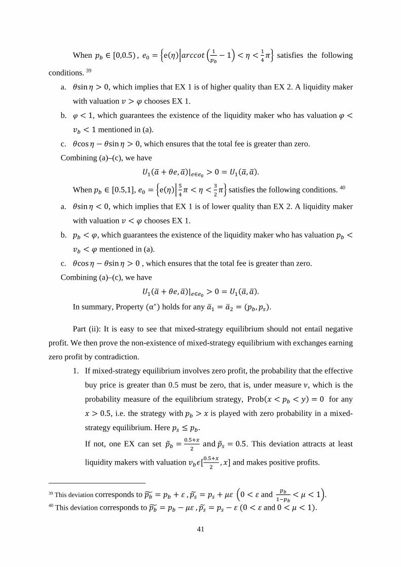
41

When 𝑝𝑝𝑏𝑏 ∈ [0,0.5) , 𝜃𝜃0 = �e(𝜂𝜂)�𝑚𝑚𝑃𝑃𝑐𝑐𝑐𝑐𝑐𝑐𝑎𝑎 � 1𝑝𝑝𝑏𝑏− 1� < 𝜂𝜂 < 1

4𝜋𝜋� satisfies the following

conditions. 39

a. 𝜃𝜃sin 𝜂𝜂 > 0, which implies that EX 1 is of higher quality than EX 2. A liquidity maker

with valuation 𝑣𝑣 > 𝜑𝜑 chooses EX 1.

b. 𝜑𝜑 < 1, which guarantees the existence of the liquidity maker who has valuation 𝜑𝜑 <

𝑣𝑣𝑏𝑏 < 1 mentioned in (a).

c. 𝜃𝜃cos 𝜂𝜂 − 𝜃𝜃sin 𝜂𝜂 > 0, which ensures that the total fee is greater than zero.

Combining (a)–(c), we have

𝑈𝑈1(𝑚𝑚� + 𝜃𝜃𝜃𝜃,𝑚𝑚�)|𝑛𝑛∈𝑛𝑛0 > 0 = 𝑈𝑈1(𝑚𝑚�,𝑚𝑚�).

When 𝑝𝑝𝑏𝑏 ∈ [0.5,1], 𝜃𝜃0 = �e(𝜂𝜂)� 54𝜋𝜋 < 𝜂𝜂 < 3

2𝜋𝜋� satisfies the following conditions. 40

a. 𝜃𝜃sin 𝜂𝜂 < 0, which implies that EX 1 is of lower quality than EX 2. A liquidity maker

with valuation 𝑣𝑣 < 𝜑𝜑 chooses EX 1.

b. 𝑝𝑝𝑏𝑏 < 𝜑𝜑, which guarantees the existence of the liquidity maker who has valuation 𝑝𝑝𝑏𝑏 <

𝑣𝑣𝑏𝑏 < 𝜑𝜑 mentioned in (a).

c. 𝜃𝜃cos 𝜂𝜂 − 𝜃𝜃sin 𝜂𝜂 > 0 , which ensures that the total fee is greater than zero.

Combining (a)–(c), we have

𝑈𝑈1(𝑚𝑚� + 𝜃𝜃𝜃𝜃,𝑚𝑚�)|𝑛𝑛∈𝑛𝑛0 > 0 = 𝑈𝑈1(𝑚𝑚�,𝑚𝑚�).

In summary, Property (α∗) holds for any 𝑚𝑚�1 = 𝑚𝑚�2 = (𝑝𝑝𝑏𝑏,𝑝𝑝𝑠𝑠).

Part (ii): It is easy to see that mixed-strategy equilibrium should not entail negative

profit. We then prove the non-existence of mixed-strategy equilibrium with exchanges earning

zero profit by contradiction.

1. If mixed-strategy equilibrium involves zero profit, the probability that the effective

buy price is greater than 0.5 must be zero, that is, under measure 𝜈𝜈, which is the

probability measure of the equilibrium strategy, Prob(𝑚𝑚 < 𝑝𝑝𝑏𝑏 < 𝑦𝑦) = 0 for any

𝑚𝑚 > 0.5, i.e. the strategy with 𝑝𝑝𝑏𝑏 > 𝑚𝑚 is played with zero probability in a mixed-

strategy equilibrium. Here 𝑝𝑝𝑠𝑠 ≤ 𝑝𝑝𝑏𝑏.

If not, one EX can set 𝑝𝑝�𝑏𝑏 = 0.5+𝑥𝑥2

and 𝑝𝑝�𝑠𝑠 = 0.5. This deviation attracts at least

liquidity makers with valuation 𝑣𝑣𝑏𝑏𝜖𝜖[0.5+𝑥𝑥2

, 𝑚𝑚] and makes positive profits.

39 This deviation corresponds to 𝑝𝑝𝑏𝑏� = 𝑝𝑝𝑏𝑏 + 𝜀𝜀 , 𝑝𝑝𝑠𝑠� = 𝑝𝑝𝑠𝑠 + 𝜇𝜇𝜀𝜀 �0 < 𝜀𝜀 and 𝑝𝑝𝑏𝑏

1−𝑝𝑝𝑏𝑏< 𝜇𝜇 < 1�.

40 This deviation corresponds to 𝑝𝑝𝑏𝑏� = 𝑝𝑝𝑏𝑏 − 𝜇𝜇𝜀𝜀 , 𝑝𝑝𝑠𝑠� = 𝑝𝑝𝑠𝑠 − 𝜀𝜀 (0 < 𝜀𝜀 and 0 < 𝜇𝜇 < 1).

42

2. If mixed-strategy equilibrium involves zero profit, the probability that the effective

buy price is smaller than 0.5 must be zero, that is, Prob(𝑚𝑚 < 𝑝𝑝𝑏𝑏 < 𝑦𝑦) = 0 for any

𝑦𝑦 < 0.5.

If not, one EX can have a profitable deviation by setting its fee structure as 𝑝𝑝�𝑏𝑏 =

0.5 ,𝑝𝑝�𝑠𝑠 = 0.5 − 𝜀𝜀 (𝜀𝜀 > 0), because (𝑝𝑝�𝑏𝑏,𝑝𝑝�𝑠𝑠) could attract some traders for any

𝑝𝑝𝑏𝑏 = 𝑝𝑝𝑠𝑠 = 𝜆𝜆 , where 𝜆𝜆 ∈ (𝑚𝑚, 𝑦𝑦) . The proof is equivalent to show that, for

sufficiently small 𝜀𝜀, we can find 𝜑𝜑 < 1 such that

(𝜑𝜑 − 0.5)(0.5 − 𝜀𝜀) = (𝜑𝜑 − 𝜆𝜆)𝜆𝜆

𝜑𝜑 =0.25 − 0.5𝜀𝜀 − 𝜆𝜆2

0.5 − 𝜀𝜀 − 𝜆𝜆

𝜑𝜑 < 1 ⇔𝜀𝜀 < 2 (0.5 − 𝜆𝜆)2

Thus we can always find 𝜀𝜀 > 0 such that 𝑝𝑝�𝑏𝑏 = 0.5 ,𝑝𝑝�𝑠𝑠 = 0.5 − 𝜀𝜀 attracts any

liquidity maker with valuation 𝑣𝑣𝑏𝑏𝜖𝜖[𝜑𝜑, 1] for any 𝑝𝑝𝑏𝑏 = 𝑝𝑝𝑠𝑠 = 𝜆𝜆 ∈ (𝑚𝑚, 𝑦𝑦). It follows

that such deviation can also outperform any 𝑝𝑝𝑏𝑏 = 𝜆𝜆 > 𝑝𝑝𝑠𝑠, because 𝑝𝑝𝑏𝑏 = 𝑝𝑝𝑠𝑠 = 𝜆𝜆

dominates any 𝑝𝑝𝑏𝑏 = 𝜆𝜆 > 𝑝𝑝𝑠𝑠 for the liquidity maker. Consequently, such a

deviation can always yield positive profit with positive probability.

3. If mixed-strategy equilibrium involves zero profit, the probability that the effective

buy price is equal to 0.5 must be zero. If not, one EX can use strategy (A.4) to

ensure itself positive profit with positive probability.

To summarize, a strategy with zero profit is strictly dominated by some other strategy,

which implies such a strategy must be played with zero probability. ■

Proof of PROPOSITION 5

i) Conditions for the Existence of Proposed Price on Grid:

Given 𝑣𝑣𝑏𝑏, when the liquidity maker can only quote on the price grids given by tick

size constraints (1′), her expected surplus is

𝐵𝐵𝐵𝐵(𝑃𝑃; 𝑣𝑣𝑏𝑏) ≡ (𝑣𝑣𝑏𝑏 − 𝑃𝑃 − 𝑓𝑓𝑚𝑚) ∙ Prob(𝑣𝑣𝑠𝑠 ≤ 𝑃𝑃 − 𝑓𝑓𝑡𝑡)

= (𝑣𝑣𝑏𝑏 − 𝑃𝑃 − 𝑓𝑓𝑚𝑚) ∙ 2 ∙ max �0, min �12

,𝑃𝑃 − 𝑓𝑓𝑡𝑡��,

where 𝑃𝑃 = 𝑛𝑛𝑁𝑁

, and 𝑛𝑛 and 𝑁𝑁 are integers.

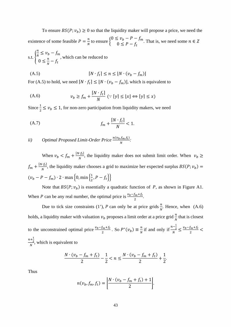
43

To ensure 𝐵𝐵𝐵𝐵(𝑃𝑃; 𝑣𝑣𝑏𝑏) ≥ 0 so that the liquidity maker will propose a price, we need the

existence of some feasible 𝑃𝑃 = 𝑛𝑛𝑁𝑁

to ensure �0 ≤ 𝑣𝑣𝑏𝑏 − 𝑃𝑃 − 𝑓𝑓𝑚𝑚0 ≤ 𝑃𝑃 − 𝑓𝑓𝑡𝑡

. That is, we need some 𝑛𝑛 ∈ 𝑍𝑍

s.t. �𝑛𝑛𝑁𝑁≤ 𝑣𝑣𝑏𝑏 − 𝑓𝑓𝑚𝑚

0 ≤ 𝑛𝑛𝑁𝑁− 𝑓𝑓𝑡𝑡

, which can be reduced to

(A.5) ⌈𝑁𝑁 ∙ 𝑓𝑓𝑡𝑡⌉ ≤ 𝑛𝑛 ≤ ⌊𝑁𝑁 ∙ (𝑣𝑣𝑏𝑏 − 𝑓𝑓𝑚𝑚)⌋

For (A.5) to hold, we need ⌈𝑁𝑁 ∙ 𝑓𝑓𝑡𝑡⌉ ≤ ⌊𝑁𝑁 ∙ (𝑣𝑣𝑏𝑏 − 𝑓𝑓𝑚𝑚)⌋, which is equivalent to

(A.6) 𝑣𝑣𝑏𝑏 ≥ 𝑓𝑓𝑚𝑚 +⌈𝑁𝑁 ∙ 𝑓𝑓𝑡𝑡⌉𝑁𝑁

(∵ ⌈𝑦𝑦⌉ ≤ ⌊𝑚𝑚⌋ ⟺ ⌈𝑦𝑦⌉ ≤ 𝑚𝑚)

Since 12≤ 𝑣𝑣𝑏𝑏 ≤ 1, for non-zero participation from liquidity makers, we need

(A.7) 𝑓𝑓𝑚𝑚 +⌈𝑁𝑁 ∙ 𝑓𝑓𝑡𝑡⌉𝑁𝑁

< 1.

ii) Optimal Proposed Limit-Order Price 𝑛𝑛(𝑣𝑣𝑏𝑏,𝑓𝑓𝑚𝑚,𝑓𝑓𝑡𝑡)𝑁𝑁

:

When 𝑣𝑣𝑏𝑏 < 𝑓𝑓𝑚𝑚 + ⌈𝑁𝑁∙𝑓𝑓𝑡𝑡⌉𝑁𝑁

, the liquidity maker does not submit limit order. When 𝑣𝑣𝑏𝑏 ≥

𝑓𝑓𝑚𝑚 + ⌈𝑁𝑁∙𝑓𝑓𝑡𝑡⌉𝑁𝑁

, the liquidity maker chooses a grid to maximize her expected surplus 𝐵𝐵𝐵𝐵(𝑃𝑃; 𝑣𝑣𝑏𝑏) =

(𝑣𝑣𝑏𝑏 − 𝑃𝑃 − 𝑓𝑓𝑚𝑚) ∙ 2 ∙ max �0, min �12

,𝑃𝑃 − 𝑓𝑓𝑡𝑡��

Note that 𝐵𝐵𝐵𝐵(𝑃𝑃; 𝑣𝑣𝑏𝑏) is essentially a quadratic function of 𝑃𝑃, as shown in Figure A1.

When 𝑃𝑃 can be any real number, the optimal price is 𝑣𝑣𝑏𝑏−𝑓𝑓𝑚𝑚+𝑓𝑓𝑡𝑡2

.

Due to tick size constraints (1’), 𝑃𝑃 can only be at price grids 𝑛𝑛𝑁𝑁

. Hence, when (A.6)

holds, a liquidity maker with valuation 𝑣𝑣𝑏𝑏 proposes a limit order at a price grid 𝑛𝑛𝑁𝑁

that is closest

to the unconstrained optimal price 𝑣𝑣𝑏𝑏−𝑓𝑓𝑚𝑚+𝑓𝑓𝑡𝑡2

. So 𝑃𝑃∗(𝑣𝑣𝑏𝑏) ≡ 𝑛𝑛𝑁𝑁

if and only if 𝑛𝑛−12𝑁𝑁≤ 𝑣𝑣𝑏𝑏−𝑓𝑓𝑚𝑚+𝑓𝑓𝑡𝑡

2<

𝑛𝑛+12𝑁𝑁

, which is equivalent to

𝑁𝑁 ∙ (𝑣𝑣𝑏𝑏 − 𝑓𝑓𝑚𝑚 + 𝑓𝑓𝑡𝑡)2

−12

< 𝑛𝑛 ≤𝑁𝑁 ∙ (𝑣𝑣𝑏𝑏 − 𝑓𝑓𝑚𝑚 + 𝑓𝑓𝑡𝑡)

2+

12

.

Thus

𝑛𝑛(𝑣𝑣𝑏𝑏,𝑓𝑓𝑚𝑚,𝑓𝑓𝑡𝑡) = �𝑁𝑁 ∙ (𝑣𝑣𝑏𝑏 − 𝑓𝑓𝑚𝑚 + 𝑓𝑓𝑡𝑡) + 1

2�.

44

FIGURE A.1

Optimal Limit-Order Price under Multiple Ticks

Notes: This figure illustrates the decision of the liquidity maker with valuation 𝑣𝑣𝑏𝑏 . The horizontal axis represents the price level and the vertical axis represents the liquidity maker’s expected surplus. Each red dot on the parabola represents a price level in the grid that gives the liquidity maker a positive expected surplus. The optimal price in the grid is the one closest to 𝑣𝑣𝑏𝑏−𝑓𝑓𝑚𝑚+𝑓𝑓𝑡𝑡

2 , which is the

liquidity maker’s optimal price without tick size constraints.

iii) Equivalence of fee structure (𝑓𝑓𝑚𝑚, 𝑓𝑓𝑡𝑡) and fee structure (𝑓𝑓𝑚𝑚, 𝑓𝑓𝑡𝑡):

For any given (𝑓𝑓𝑚𝑚,𝑓𝑓𝑡𝑡), we have 𝑛𝑛(𝑣𝑣𝑏𝑏,𝑓𝑓𝑚𝑚,𝑓𝑓𝑡𝑡) = �𝑁𝑁∙(𝑣𝑣−𝑓𝑓𝑚𝑚+𝑓𝑓𝑡𝑡)+12

�, and thus the cum fee

buy and sell prices are 𝑝𝑝𝑏𝑏 = 𝑛𝑛(𝑣𝑣𝑏𝑏,𝑓𝑓𝑚𝑚,𝑓𝑓𝑡𝑡)𝑁𝑁

+ 𝑓𝑓𝑚𝑚, and 𝑝𝑝𝑠𝑠 = 𝑛𝑛(𝑣𝑣𝑏𝑏,𝑓𝑓𝑚𝑚,𝑓𝑓𝑡𝑡)𝑁𝑁

− 𝑓𝑓𝑡𝑡.

Now consider (𝑓𝑓𝑚𝑚,𝑓𝑓𝑡𝑡), where �𝑓𝑓𝑚𝑚 = 𝑓𝑓𝑚𝑚 + 𝑘𝑘

𝑁𝑁

𝑓𝑓𝑡𝑡 = 𝑓𝑓𝑡𝑡 −𝑘𝑘𝑁𝑁

, 𝑘𝑘 ∈ 𝑍𝑍. Under (𝑓𝑓𝑚𝑚, 𝑓𝑓𝑡𝑡), 𝑛𝑛�𝑣𝑣𝑏𝑏,𝑓𝑓𝑚𝑚,𝑓𝑓𝑡𝑡� =

�𝑁𝑁∙�𝑣𝑣−�̃�𝑓𝑚𝑚+�̃�𝑓𝑡𝑡�+12

� = �𝑁𝑁∙(𝑣𝑣−𝑓𝑓𝑚𝑚+𝑓𝑓𝑡𝑡)+12

− 𝑘𝑘� = 𝑛𝑛(𝑣𝑣𝑏𝑏,𝑓𝑓𝑚𝑚, 𝑓𝑓𝑡𝑡) − 𝑘𝑘 . It follows that 𝑝𝑝�𝑏𝑏 = 𝑛𝑛�𝑣𝑣𝑏𝑏,�̃�𝑓𝑚𝑚,�̃�𝑓𝑡𝑡�𝑁𝑁

+

𝑓𝑓𝑚𝑚 = 𝑛𝑛(𝑣𝑣𝑏𝑏,𝑓𝑓𝑚𝑚,𝑓𝑓𝑡𝑡)𝑁𝑁

− 𝑘𝑘𝑁𝑁

+ 𝑓𝑓𝑚𝑚 + 𝑘𝑘𝑁𝑁

= 𝑝𝑝𝑏𝑏, and 𝑝𝑝�𝑠𝑠 = 𝑛𝑛�𝑣𝑣𝑏𝑏,�̃�𝑓𝑚𝑚,�̃�𝑓𝑡𝑡�𝑁𝑁

− 𝑓𝑓𝑡𝑡 = 𝑛𝑛(𝑣𝑣𝑏𝑏,𝑓𝑓𝑚𝑚,𝑓𝑓𝑡𝑡)𝑁𝑁

− 𝑘𝑘𝑁𝑁− 𝑓𝑓𝑡𝑡 + 𝑘𝑘

𝑁𝑁= 𝑝𝑝𝑠𝑠 .

Since, for any given 𝑣𝑣𝑏𝑏, the cum fee buy and sell prices are the same under the fee structure

(𝑓𝑓𝑚𝑚,𝑓𝑓𝑡𝑡) and the fee structure (𝑓𝑓𝑚𝑚,𝑓𝑓𝑡𝑡), these fee structures are equivalent for the liquidity maker,

the liquidity taker and EXs.

45

Proof of PROPOSITION 6

We prove this proposition through contradiction. It is easy to see that no exchange

should take a negative profit in pure-strategy equilibrium, because the operator can simply shut

down the exchange. The proof is then divided into two steps.

Step 1: No exchange should take a positive profit in pure-strategy equilibrium.

Suppose not: denote the total number of EXs that take positive profits as 𝐻𝐻. As we

have more than one operator, we can always find an operator 𝑗𝑗 who does not own all 𝐻𝐻

exchanges, that is, her profit is lower than the combined profits of these 𝐻𝐻 exchanges.

Operator 𝑗𝑗 can increase her profits by establishing 𝐻𝐻 additional EXs to undercut each

of the existing profitable EXs with the following fee structure:

𝑓𝑓𝑚𝑚𝑖𝑖ℎ = 𝑓𝑓𝑚𝑚ℎ − 𝜀𝜀 and 𝑓𝑓𝑡𝑡

𝑖𝑖ℎ = 𝑓𝑓𝑡𝑡ℎ, for ℎ = 1,2,3,⋯ ,𝐻𝐻.

Such a deviation allows operator j to capture the entire market. Therefore, step 1

requires all exchanges to take a zero profit in pure-strategy equilibrium.

Step 2: It is impossible for all exchanges to have zero profit in pure-strategy equilibrium.

Suppose that all operators have zero profit. We can rank the feasible cum fee sell prices

in equilibrium as 𝑝𝑝𝑠𝑠1 < 𝑝𝑝𝑠𝑠2 < ⋯ < 𝑝𝑝𝑠𝑠𝑄𝑄, where Q is the number of feasible cum fee sell prices in

all exchanges.

Similar to case (ii-b) in Proposition 3, two subcases are to be considered: (I) 𝑝𝑝𝑏𝑏1 = 𝑝𝑝𝑠𝑠1 =

𝛾𝛾 < 12; (II) 𝑝𝑝𝑏𝑏1 = 𝑝𝑝𝑠𝑠1 = 𝛾𝛾 ≥ 1

2. 41 In (I), operator 𝑗𝑗 can open a new EX using strategy (A.3) to

ensure herself positive profits at positive probability. In (II), operator 𝑗𝑗 can open a new EX

using strategy (A.4) to ensure herself positive profits at positive probability.

Combining Steps 1–2, the proposition follows. ■

Proof of PROPOSITION 7

We prove the proposition using the example of two exchanges, and the results for

multiple exchanges follow directly.

Charging One Side Only:

41 Under multiple tick sizes, there are multiple cum fee sell prices that are determined by both the take fees and the liquidity maker’s limit-order price. Such multiplicity does not affect the proof, because we need only a profitable deviation from the EX with the lowest cum fee sell price.

46

Here we consider the case in which only the liquidity taker is charged fees, and the

liquidity maker is not charged, that is,

𝑓𝑓𝑚𝑚𝑖𝑖 = 0 and 𝑓𝑓𝑡𝑡𝑖𝑖 ≥ 0.

The case in which 𝑓𝑓𝑚𝑚𝑖𝑖 ≥ 0, and 𝑓𝑓𝑡𝑡𝑖𝑖 = 0 can be proved similarly.

Recall that �𝑝𝑝𝑏𝑏𝑖𝑖 = 𝑃𝑃𝑖𝑖 + 𝑓𝑓𝑚𝑚𝑖𝑖

𝑝𝑝𝑠𝑠𝑖𝑖 = 𝑃𝑃𝑖𝑖 − 𝑓𝑓𝑡𝑡𝑖𝑖. When the rebate to the liquidity maker is banned, the

liquidity maker’s maximal surplus under (0,𝑓𝑓𝑡𝑡𝑖𝑖) becomes

𝐵𝐵𝐵𝐵𝑖𝑖∗�𝑣𝑣𝑏𝑏;𝑓𝑓𝑡𝑡𝑖𝑖� = max𝑃𝑃𝑖𝑖

��𝑣𝑣𝑏𝑏 − 𝑃𝑃𝑖𝑖� ∙ min {1,2�𝑃𝑃𝑖𝑖 − 𝑓𝑓𝑡𝑡𝑖𝑖�}�𝑣𝑣𝑏𝑏 − 𝑃𝑃𝑖𝑖 ≥ 0 and 𝑃𝑃𝑖𝑖 − 𝑓𝑓𝑡𝑡𝑖𝑖 ≥ 0�.

For any 𝑓𝑓𝑡𝑡1 ≥ 𝑓𝑓𝑡𝑡2 ≥ 0, we must have

(A.8) 𝐵𝐵𝐵𝐵𝑖𝑖∗(𝑣𝑣𝑏𝑏; 𝑓𝑓𝑡𝑡1) ≤ 𝐵𝐵𝐵𝐵𝑖𝑖∗(𝑣𝑣𝑏𝑏;𝑓𝑓𝑡𝑡2) for any 𝑣𝑣𝑏𝑏.

Thus, any liquidity maker chooses the EX with the lowest take fee, if she chooses to trade.

Then exchanges compete to undercut each other in take fee, which yields a Bertrand outcome.

Equal Splitting the Total Fee:

Now we consider the case in which the total fee is equally split between a liquidity

maker and a liquidity taker, that is,

𝑓𝑓𝑚𝑚𝑖𝑖 = 𝑓𝑓𝑡𝑡𝑖𝑖 =𝑇𝑇𝑖𝑖

2≥ 0.

The liquidity maker’s maximal surplus under (𝑇𝑇𝑖𝑖

2, 𝑇𝑇

𝑖𝑖

2) is

𝐵𝐵𝐵𝐵𝑖𝑖∗�𝑣𝑣𝑏𝑏;𝑇𝑇𝑖𝑖�

= max𝑃𝑃𝑖𝑖

��𝑣𝑣𝑏𝑏 − 𝑃𝑃𝑖𝑖 − 𝑇𝑇𝑖𝑖2 � ∙ min {1,2 �𝑃𝑃𝑖𝑖 − 𝑇𝑇𝑖𝑖

2 �}�𝑣𝑣𝑏𝑏 − 𝑃𝑃𝑖𝑖 − 𝑇𝑇𝑖𝑖2 ≥ 0 and 𝑃𝑃𝑖𝑖 − 𝑇𝑇𝑖𝑖

2 ≥ 0� .

For any 𝑇𝑇1 ≥ 𝑇𝑇2 ≥ 0, we must have

𝐵𝐵𝐵𝐵𝑖𝑖∗(𝑣𝑣𝑏𝑏;𝑇𝑇1) ≤ 𝐵𝐵𝐵𝐵𝑖𝑖∗(𝑣𝑣𝑏𝑏;𝑇𝑇2) for any 𝑣𝑣𝑏𝑏.

Thus, any liquidity maker chooses the EX with the lowest 𝑇𝑇𝑖𝑖, if she chooses to trade. Then

the competition between exchanges yields a Bertrand outcome. ■

47

APPENDIX B: FEE STRUCTURE UNDER MULTIPLE TICKS

Here we present the optimal fee structure and profit as a function of 𝑁𝑁 when 𝑁𝑁 > 8.

When the value of N is between 2 and 8, the optimal solutions are discussed on a case-by-case

basis, the results of which are available upon request.

PROPOSITION B1 (monopoly fee structure under multiple ticks). Under tick size constraints

(1′), for 𝑁𝑁 > 8, the following fee structure maximizes the profit:

𝑓𝑓𝑚𝑚∗ = −𝑛𝑛𝑁𝑁

+7𝑁𝑁2 + 8𝑁𝑁 + 𝑃𝑃 ∙ (4 − 𝑃𝑃)

16𝑁𝑁2

𝑓𝑓𝑡𝑡∗ =𝑛𝑛𝑁𝑁−𝑁𝑁2 + 8𝑁𝑁 − 𝑃𝑃 ∙ (4 − 𝑃𝑃)

16𝑁𝑁2

where 𝑛𝑛𝑁𝑁

is the proposed limit-order price at 𝑣𝑣𝑏𝑏 = 12

, i.e., 𝑛𝑛 ≡ �𝑁𝑁�12−𝑓𝑓𝑚𝑚+𝑓𝑓𝑡𝑡�+1

2� , and 𝑃𝑃 ∈

{0,1,2,3} is the remainder of 𝑁𝑁 divided by 4.

The maximum profit of the monopoly exchange is:

𝛱𝛱∗(𝑓𝑓𝑚𝑚∗ ,𝑓𝑓𝑡𝑡∗) = �38

+ 𝑟𝑟∙(4−𝑟𝑟)8𝑁𝑁2

�2,

and 𝑙𝑙𝑖𝑖𝑚𝑚𝑁𝑁→∞

𝛱𝛱∗(𝑓𝑓𝑚𝑚∗ ,𝑓𝑓𝑡𝑡∗) = 964

.

We prove this proposition in three steps.

Step 1: Notations and Preliminary Analysis

Denote the sum and difference between the make and take fees, respectively, as

𝑇𝑇 ≡ 𝑓𝑓𝑚𝑚 + 𝑓𝑓𝑡𝑡 , and 𝐷𝐷 ≡ 𝑓𝑓𝑚𝑚 − 𝑓𝑓𝑡𝑡 .

Note that the optimal make and take fees (𝑓𝑓𝑚𝑚,𝑓𝑓𝑡𝑡) follow directly from 𝑇𝑇 and 𝐷𝐷.

A liquidity maker with valuation within [𝜑𝜑𝑛𝑛,𝜑𝜑𝑛𝑛+1] proposes a limit order at price 𝑃𝑃 =𝑛𝑛𝑁𝑁

. To find the threshold 𝜑𝜑𝑛𝑛, we need

�𝜑𝜑𝑛𝑛 − 𝑓𝑓𝑚𝑚 −𝑛𝑛 − 1𝑁𝑁 ��−𝑓𝑓𝑡𝑡 +

𝑛𝑛 − 1𝑁𝑁 � = �𝜑𝜑𝑛𝑛 − 𝑓𝑓𝑚𝑚 −

𝑛𝑛𝑁𝑁� �−𝑓𝑓𝑡𝑡 +

𝑛𝑛𝑁𝑁�.

Thus

𝜑𝜑𝑛𝑛 = 𝑓𝑓𝑚𝑚 − 𝑓𝑓𝑡𝑡 +2𝑛𝑛 − 1𝑁𝑁

= 𝐷𝐷 +2𝑛𝑛 − 1𝑁𝑁

.

It follows that

48

𝜑𝜑𝑛𝑛+1 − 𝜑𝜑𝑛𝑛 =2𝑁𝑁

.

Therefore, the length of a complete interval [𝜑𝜑𝑛𝑛,𝜑𝜑𝑛𝑛+1] for liquidity makers who propose the

same limit-order price is 2𝑁𝑁

.

For now, we assume that any liquidity maker with valuation 𝑣𝑣𝑏𝑏 ∈ [12

, 1] participates in

trading. We verify that such a condition is satisfied when 𝑁𝑁 > 8. Full participation implies that

the number of complete intervals contained in [12

, 1] is�1−122𝑁𝑁� = �𝑁𝑁

4� = �𝑧𝑧 + 𝑟𝑟

4� = 𝑧𝑧, where 𝑁𝑁 =

4𝑧𝑧 + 𝑃𝑃, 𝑧𝑧 is a non-negative integer, and 𝑃𝑃 ∈ {0,1,2,3} is the remainder of 𝑁𝑁 divided by 4.

We denote the number of thresholds (𝜑𝜑𝑛𝑛) contained in [12

, 1] as 𝑚𝑚 , noting that the

thresholds closest to two ends of [12

, 1] may be from incomplete intervals. Then 𝑚𝑚 can only be

𝑧𝑧 or 𝑧𝑧 + 1, as illustrated in Figure B1, where 𝑛𝑛𝑁𝑁

is the proposed price for 𝑣𝑣𝑏𝑏 = 12, i.e., 𝑛𝑛 ≡

�𝑁𝑁�12−𝑓𝑓𝑚𝑚+𝑓𝑓𝑡𝑡�+1

2�.

Step 2: Optimal Fee Breakdown D for Given 𝑻𝑻

For any given 𝑇𝑇, suppose 𝐷𝐷∗ ≡ argmax𝐷𝐷

Π(𝐷𝐷;𝑇𝑇). Then any disturbance ∆ on 𝐷𝐷∗ such

that 𝐷𝐷� = 𝐷𝐷∗ + 2∆ (i.e., 𝑓𝑓𝑚𝑚 = 𝑓𝑓𝑚𝑚∗ + ∆ and 𝑓𝑓𝑡𝑡 = 𝑓𝑓𝑡𝑡∗ − ∆) should not improve profits. Under the

new fee structure �𝑇𝑇,𝐷𝐷�� (or equivalently, 𝑓𝑓𝑚𝑚 = 𝑓𝑓𝑚𝑚∗ + ∆ and 𝑓𝑓𝑡𝑡 = 𝑓𝑓𝑡𝑡∗ − ∆), all thresholds have

been shifted by 2∆, that is,

𝜑𝜑�𝑛𝑛 = 𝜑𝜑𝑛𝑛∗ + 2∆.

There are two cases to be considered:

(i) 𝑃𝑃 ≠ 0

If ∆> 0, all thresholds 𝜑𝜑�𝑛𝑛 shift toward the right, compared with 𝜑𝜑𝑛𝑛∗ . For each original

interval [𝜑𝜑𝑛𝑛∗ , 𝜑𝜑𝑛𝑛+1∗ ], 2∆ liquidity makers reduce their quotes by one tick (1𝑁𝑁

). As a result, the

EX’s execution probability for these liquidity makers decreases by 2𝑁𝑁

. Since there are 𝑚𝑚

thresholds, the aggregate profit loss for the EX is 𝑇𝑇 ∙ 𝑥𝑥∙2∆1−12

∙ 2𝑁𝑁

= 2∆𝑇𝑇 ∙ 4𝑥𝑥𝑁𝑁

.

At the same time, for the whole interval [12

, 1] , a decrease in 𝑓𝑓𝑡𝑡 �recall that

𝑓𝑓𝑡𝑡 = 𝑓𝑓𝑡𝑡∗ − ∆� increases the execution probability by 2∆. It yields a profit gain for the EX of 𝑇𝑇 ∙

1−121−12

∙ 2∆= 2∆𝑇𝑇.

49

In panels (b) and (c) of Figure B1, there are 𝑧𝑧 effective thresholds when all thresholds

𝜑𝜑�𝑛𝑛 shift toward the right (∆> 0). Since 4𝑥𝑥𝑁𝑁

= 4𝑧𝑧𝑁𝑁

< 1 , a deviation of ∆> 0 increases the EX’s

total profit. So the cases presented in panels (b) and (c) cannot be optimal.

FIGURE B1

Disturbance on Fee Breakdown

Similarly, the cases presented in panels (a) and (b) cannot be optimal, because ∆< 0

leads to higher profit when 𝑚𝑚 = 𝑧𝑧 + 1. As a result, only the case in panel (d) can be optimal.

So at optimal, we have 𝜑𝜑𝑛𝑛 = 12.

(ii) 𝑃𝑃 = 0

50

We have 𝑚𝑚 = 𝑧𝑧 and thus 2∆𝑇𝑇 ∙ 4𝑥𝑥𝑁𝑁

= 2∆𝑇𝑇 ∙ 4𝑧𝑧𝑁𝑁

= 2∆𝑇𝑇, because 𝑁𝑁 = 4𝑧𝑧. Thus, a small

disturbance ∆ has no effect on the EX’s profit. Therefore, fee breakdown happens to be neutral

for a monopoly EX when 𝑃𝑃 = 0. Without loss of generality, we assume 𝜑𝜑𝑛𝑛 = 12, so that we can

use the same formula for any 𝑁𝑁 > 8.42

Combining (i) and (ii) above, at optimum, we must have 𝑛𝑛 = �𝑁𝑁�12−𝑓𝑓𝑚𝑚+𝑓𝑓𝑡𝑡�+1

2� such

that 𝜑𝜑𝑛𝑛 = 𝐷𝐷 + 2𝑛𝑛−1𝑁𝑁

= 12. This condition implies that 𝐷𝐷 = 1

2− 2𝑛𝑛−1

𝑁𝑁. It follows that

𝑓𝑓𝑚𝑚 =𝑇𝑇 + 𝐷𝐷

2=𝑇𝑇 −

2𝑛𝑛 − 1𝑁𝑁 + 1

22

, 𝑓𝑓𝑡𝑡 =𝑇𝑇 − 𝐷𝐷

2=𝑇𝑇 +

2𝑛𝑛 − 1𝑁𝑁 − 1

22

.

Step 3: Determination of Optimal 𝑻𝑻

When any liquidity maker with valuation 𝑣𝑣𝑏𝑏 ∈ [12

, 1] submits a limit order, the EX’s

expected profit depends on the total fee and the limit order’s execution probability.

𝛱𝛱(𝑓𝑓𝑚𝑚,𝑓𝑓𝑡𝑡) = total fee × � (execution probability × interval width)all price levels

= 𝑇𝑇 ∙ 2 ∙ � � �−𝑓𝑓𝑡𝑡 +𝑖𝑖𝑁𝑁�

𝑧𝑧+𝑛𝑛−1

𝑖𝑖=𝑛𝑛

∙2𝑁𝑁

1 − 12

+ �−𝑓𝑓𝑡𝑡 +𝑧𝑧 + 𝑛𝑛𝑁𝑁 � ∙

𝑃𝑃2𝑁𝑁

1 − 12�

= 𝑇𝑇 ∙ �34

+𝑃𝑃 ∙ (4 − 𝑃𝑃)

4𝑁𝑁2 − 𝑇𝑇�

Thus,

𝑇𝑇∗ =38

+𝑃𝑃 ∙ (4 − 𝑃𝑃)

8𝑁𝑁2 , and 𝛱𝛱∗ = �38

+𝑃𝑃 ∙ (4 − 𝑃𝑃)

8𝑁𝑁2 �2

.

The optimal fees follow directly as

𝑓𝑓𝑚𝑚∗ =𝑇𝑇∗ + 𝐷𝐷∗

2= −

𝑛𝑛𝑁𝑁

+7𝑁𝑁2 + 8𝑁𝑁 + 𝑃𝑃 ∙ (4 − 𝑃𝑃)

16𝑁𝑁2

𝑓𝑓𝑡𝑡∗ =𝑇𝑇∗ − 𝐷𝐷∗

2=𝑛𝑛𝑁𝑁−𝑁𝑁2 + 8𝑁𝑁 − 𝑃𝑃 ∙ (4 − 𝑃𝑃)

16𝑁𝑁2 .

This proof requires the full participation of liquidity makers even after we increase the

make fee by an amount ∆> 0 . This full participation requires the liquidity maker with

42 Yet we are aware that, for 𝑃𝑃 = 0, Proposition B1 only presents one set of fees that maximize the profit. When N is the multiple of 4, the fee breakdown happens to be neutral and the optimal fee and profit coincides with the case of zero tick size under one (monopoly) exchange. Yet Table II shows that fee breakdown is no longer neutral when the monopoly operator establishes two exchanges, and Proposition 6 shows that no pure strategy exists for any tick size N.

51

valuation 𝑣𝑣𝑏𝑏 = 12 to quote a limit-order price such that the cum fee sell price is larger than 1

𝑁𝑁. If

not, an increase in make fee leads the liquidity maker with 𝑣𝑣𝑏𝑏 = 12 to quote a price one tick

lower because she is at the threshold, which leads to a cum fee sell price no larger than

zero. Because no liquidity taker accepts a negative cum fee sell price, the full participation

condition is violated. Therefore, we need

𝑝𝑝𝑠𝑠∗ = −𝑓𝑓𝑎𝑎

∗ + 𝑛𝑛𝑁𝑁

=𝑁𝑁2 + 8𝑁𝑁 − 𝑃𝑃 ∙ (4 − 𝑃𝑃)

16𝑁𝑁2 > 1𝑁𝑁

,

which reduces to 𝑁𝑁 > 8. ■

52

REFERENCES

Ambrus, Attila, and Rossella Argenziano, “Asymmetric Networks in Two-Sided Markets,” American Economic Journal: Microeconomics, 1 (2009), 1752.

Angel, James, Lawrence Harris, and Chester Spatt, “Equity Trading in the 21st Century,” Working paper, Marshall School of Business, 2010.

–––––––, Lawrence Harris, and Chester Spatt, “Equity Trading in the 21st Century: An Update,” Working paper, Marshall School of Business, 2013.

Anshuman, V. Ravi, and Avner Kalay. "Market making with discrete prices," Review of Financial Studies, 11 (1998), 81-109.

Baldauf, Markus, and Joshua Mollner, “High-Frequency Trading and Market Performance,” Working paper, University of British Columbia and Microsoft Corporation, 2015.

Battalio, Robert H., Shane A. Corwin, and Robert H. Jennings, “Can Brokers Have It All? On the Relation between Make Take Fees & Limit Order Execution Quality,” Working paper, University of Notre Dame and Indiana University Bloomington, 2015.

Baye, Michael R., John Morgan, “Information Gatekeepers on the Internet and the Competitiveness of Homogeneous Product Markets,” American Economic Reviews, 91 (2001), 454–474.

Biais, Bruno, Larry Glosten, and Chester Spatt, “Market Microstructure: A Survey of Microfoundations, Empirical Results, and Policy Implications,” Journal of Financial Markets, 8 (2005), 217–264.

Budish, Eric, Peter Cramton and John Shim, “The High-Frequency Trading Arms Race: Frequent Batch Auctions as a Market Design Response,” The Quarterly Journal of Economics, 130, (2015), 1547–1621.

Buti, Sabrina, Francesco Consonni, Barbara Rindi, Yuanji Wen, and Ingrid M. Werner, “Tick Size: Theory and Evidence,” Working paper, University of Toronto, 2014.

Burdett, Kenneth, Kenneth Judd, “Equilibrium Price Dispersion,” Econometrica, 51 (1983), 955969

Butters, Gerard R., “Equilibrium Distributions of Sales and Advertising Prices,” The Review of Economic Studies, 3 (1977), 465–491.

Cantillon, Estelle, and Pai-Ling Yin, “Competition between Exchanges: Lessons from the Battle of the Bund,” Working paper, MIT, 2008.

Cardella, Laura, Jia Hao, and Ivalina Kalcheva, “Make and Take Fees in the U.S. Equity Market,” Working paper, Texas Tech University, 2015.

Chowdhry, Bhagwan, and Vikram Nanda, “Multimarket Trading and Market Liquidity,” Review of Financial Studies, 4 (1991), 483511.

Colliard, Jean-Edouard, and Thierry Foucault, “Trading Fees and Efficiency in Limit Order Markets,” Review of Financial Studies, 25 (2012), 3389–3421.

53

Dasgupta, Partha, and Eric Maskin, “The Existence of Equilibrium in Discontinuous Economic Games, II: Applications,” The Review of Economic Studies, 53 (1986), 27–41.

Dolgopolov, Stanislav, “The Maker-Taker Pricing Model and Its Impact on the Securities Market Structure: A Can of Worms for Securities Fraud?” Virginia Law & Business Review, 8 (2014), 231–272.

Foucault, Thierry, “Pricing Liquidity in Electronic Markets,” United Kingdom Government Office of Science, Foresight Projects, 2012.

–––––––, and Albert Menkveld, “Competition for Order Flow and Smart Order Routing Systems,” Journal of Finance, 63 (2008), 119–158.

–––––––, and Christine A. Parlour, “Competition for Listings,” The RAND Journal of Economics, 35 (2004), 329–355.

–––––––, Ohad Kadan, and Eugene Kandel, “Liquidity Cycles and Make/Take Fees in Electronic Markets,” Journal of Finance, 68 (2013), 299–341.

–––––––, Roman Kozhan, and Wing Wah Tham, “Toxic Arbitrage,” Working paper, HEC Pairs, University of Warwick and Erasmus School of Economics, 2015.

Glosten, Lawrence, “Is the Electronic Open Limit Order Book Inevitable?,” Journal of Finance, 49 (1994), 1127–1161.

Hagiu, Andrei, Julian Wright, “Multisided Platforms,” International Journal of Industrial Organization, 43 (2015), 162-174.

Kandel, Eugene, and Leslie M. Marx. "Nasdaq market structure and spread patterns." Journal of Financial Economics 45 (1997): 61-89.

Kwan, Amy, Ronald Masulis, and Thomas H. Mclnish, “Trading Rules, Competition for Order Flow and Market Fragmentation,” Journal of Financial Economics, 115 (2015), 330–348.

Lewis, Michael, Flash Boys: A Wall Street Revolt, New York, London, W. W. Norton & Company, 2014.

Madhavan, Ananth, “Exchange-Traded Funds, Market Structure and the Flash Crash,” Financial Analysts Journal, 68 (2012), 20–35.

Malinova, Katya, and Andreas Park. “Subsidizing liquidity: The impact of make/take fees on market quality.” Journal of Finance, 70 (2015), 509-536.

Menkveld, Albert J., “High Frequency Trading and The New-Market Makers,” Working Paper, VU University Amsterdam, 2010.

Mussa, Michael, and Sherwin Rose, “Monopoly and Product Quality,” Journal of Economic Theory, 18 (1978), 301–317.

O’Donoghue, Shawn M., “The Effect of Maker-Taker Fees on Investor Order Choice and Execution Quality in U.S. Stock Markets,” Working paper, Indiana University, 2015.

54

O’Hara, Maureen, and Mao Ye, “Is Market Fragmentation Harming Market Quality?,” Journal of Finance Economics, 100 (2011), 459–474.

–––––––, G. Saar, and Z. Zhong, “Relative Tick Size and the Trading Environment,” unpublished Working paper, Cornell University, 2015.

Pagano, Marco, “Trading Volume and Asset Liquidity,” The Quarterly Journal of Economics, 104 (1989), 255–274.

Pagnotta, Emiliano S., and Thomas Philippon, “Competing on Speed,” Working paper, New York University, 2015.

Parlour, Christine, and Duane Seppi, “Liquidity-Based Competition for Order Flow,” Review of Financial Studies, 16 (2003), 301–343.

Rochet, Jean-Charles, Jean Tirole, “Two-Sided Markets: A Progress Report,” The RAND Journal of Economics, 37 (2006), 645-667.

Rosenthal, Robert W., “A Model in which an Increase in the Number of Sellers Leads to a Higher Price,” Econometrica, 48 (1980), 1575–1579.

Rosu, Ioanid, “A Dynamic Model of the Limit Order Book,” Review of Financial Studies, 22 (2009), 4601–4641.

Rysman, Marc, “The Economics of Two-Sided Markets,” Journal of Economic Perspective, 25 (2009), 125–143.

Santos, Tano, and José A. Scheinkman, “Competition among Exchanges,” Quarterly Journal of Economics, 116 (2001), 1027–1061.

Securities and Exchange Commission (SEC) Division of Trading and Markets Memorandum to SEC Market Structure Advisory Committee (“Committee”), Washington, DC, October 20, 2015.

Shaked, Avner, and John Sutton, “Relaxing Price Competition through Product Differentiation,” Review of Economic Studies, 49 (1982), 3–13.

Stigler, George J., “Public Regulation of Securities Markets,” Journal of Business, 37 (1964), 117–142.

Tirole, Jean, “The Theory of Industrial Organization,” The MIT Press, 1988.

Weild, David, Edward Kim, and Lisa Newport, “The Trouble with Small Tick Sizes,” Working paper, Grant Thornton, 2012.

Weyl, E Glen, “A Price Theory of Multi-sided Platforms,” American Economic Review, 100 (2010): 1642–1672.

Varian, Hal R., “A Model of Sales,” American Economic Review, 70 (1980), 651–659.

Yao, Chen, and Mao Ye, “Why Trading Speed Matters: A Tale of Queue Rationing under Price Controls,” Working paper, University of Warwick and University of Illinois at Urbana-Champaign, 2015.

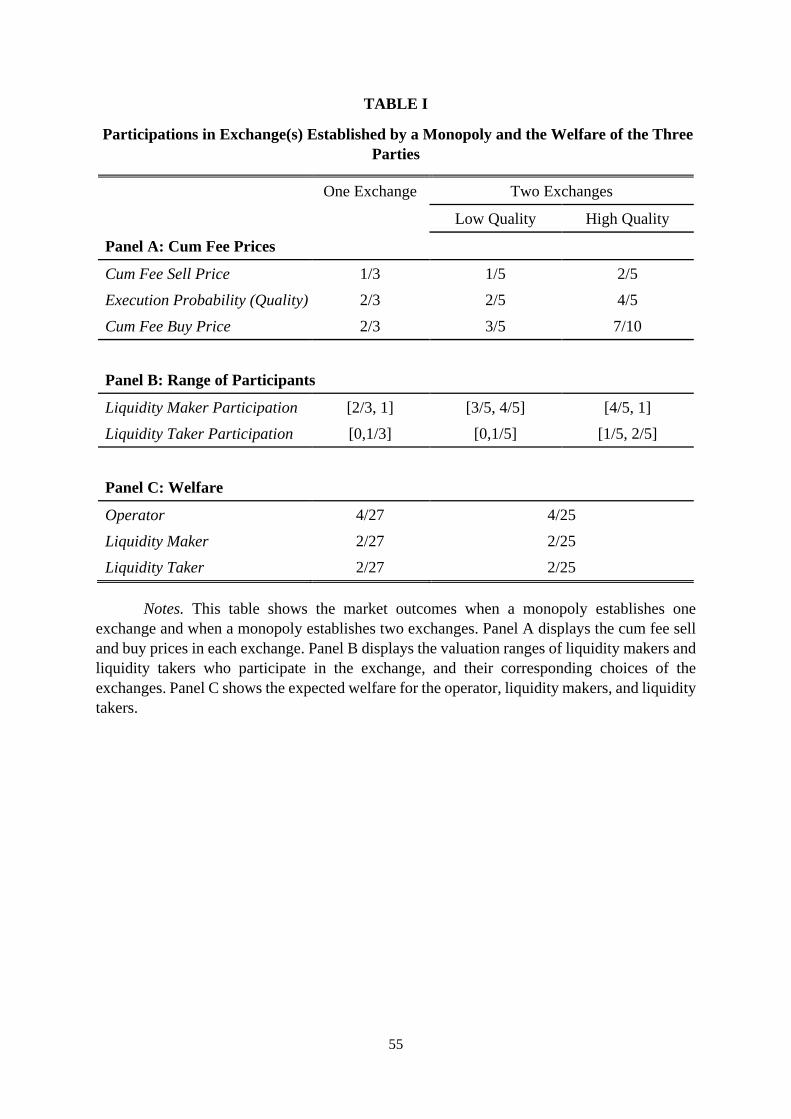
55

TABLE I

Participations in Exchange(s) Established by a Monopoly and the Welfare of the Three Parties

One Exchange Two Exchanges

Low Quality High Quality

Panel A: Cum Fee Prices

Cum Fee Sell Price 1/3 1/5 2/5 Execution Probability (Quality) 2/3 2/5 4/5 Cum Fee Buy Price 2/3 3/5 7/10

Panel B: Range of Participants

Liquidity Maker Participation [2/3, 1] [3/5, 4/5] [4/5, 1] Liquidity Taker Participation [0,1/3] [0,1/5] [1/5, 2/5]

Panel C: Welfare

Operator 4/27 4/25 Liquidity Maker 2/27 2/25 Liquidity Taker 2/27 2/25

Notes. This table shows the market outcomes when a monopoly establishes one exchange and when a monopoly establishes two exchanges. Panel A displays the cum fee sell and buy prices in each exchange. Panel B displays the valuation ranges of liquidity makers and liquidity takers who participate in the exchange, and their corresponding choices of the exchanges. Panel C shows the expected welfare for the operator, liquidity makers, and liquidity takers.

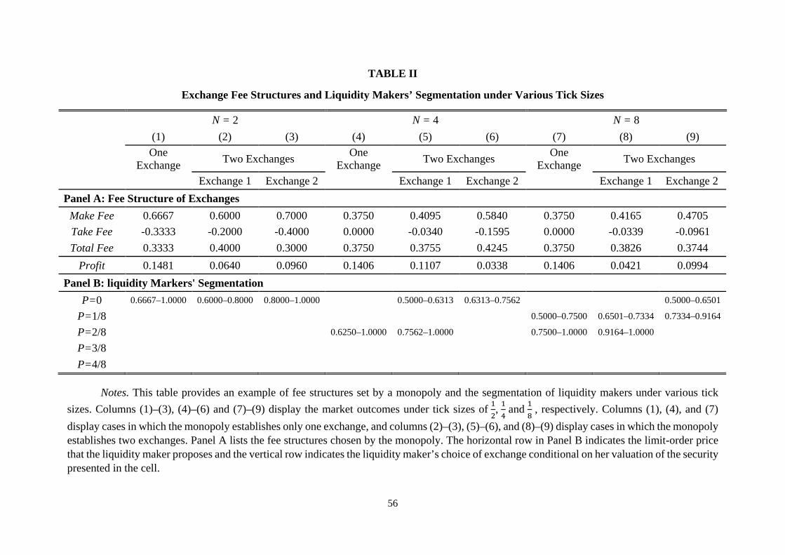
56

TABLE II

Exchange Fee Structures and Liquidity Makers’ Segmentation under Various Tick Sizes

N = 2 N = 4 N = 8 (1) (2) (3) (4) (5) (6) (7) (8) (9)

One Exchange Two Exchanges One

Exchange Two Exchanges One Exchange Two Exchanges

Exchange 1 Exchange 2 Exchange 1 Exchange 2 Exchange 1 Exchange 2 Panel A: Fee Structure of Exchanges

Make Fee 0.6667 0.6000 0.7000 0.3750 0.4095 0.5840 0.3750 0.4165 0.4705 Take Fee -0.3333 -0.2000 -0.4000 0.0000 -0.0340 -0.1595 0.0000 -0.0339 -0.0961 Total Fee 0.3333 0.4000 0.3000 0.3750 0.3755 0.4245 0.3750 0.3826 0.3744

Profit 0.1481 0.0640 0.0960 0.1406 0.1107 0.0338 0.1406 0.0421 0.0994 Panel B: liquidity Markers' Segmentation

P=0 0.6667–1.0000 0.6000–0.8000 0.8000–1.0000 0.5000–0.6313 0.6313–0.7562 0.5000–0.6501

P=1/8 0.5000–0.7500 0.6501–0.7334 0.7334–0.9164

P=2/8 0.6250–1.0000 0.7562–1.0000 0.7500–1.0000 0.9164–1.0000

P=3/8

P=4/8

Notes. This table provides an example of fee structures set by a monopoly and the segmentation of liquidity makers under various tick sizes. Columns (1)–(3), (4)–(6) and (7)–(9) display the market outcomes under tick sizes of 1

2, 14 and 1

8 , respectively. Columns (1), (4), and (7)

display cases in which the monopoly establishes only one exchange, and columns (2)–(3), (5)–(6), and (8)–(9) display cases in which the monopoly establishes two exchanges. Panel A lists the fee structures chosen by the monopoly. The horizontal row in Panel B indicates the limit-order price that the liquidity maker proposes and the vertical row indicates the liquidity maker’s choice of exchange conditional on her valuation of the security presented in the cell.

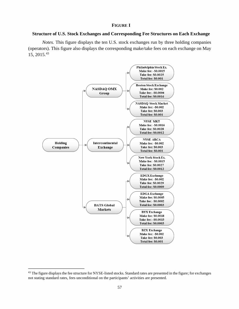
57

FIGURE I

Structure of U.S. Stock Exchanges and Corresponding Fee Structures on Each Exchange

Notes. This figure displays the ten U.S. stock exchanges run by three holding companies (operators). This figure also displays the corresponding make/take fees on each exchange on May 15, 2015.43

43 The figure displays the fee structure for NYSE-listed stocks. Standard rates are presented in the figure; for exchanges not stating standard rates, fees unconditional on the participants’ activities are presented.

58

FIGURE II

Timeline of the Model

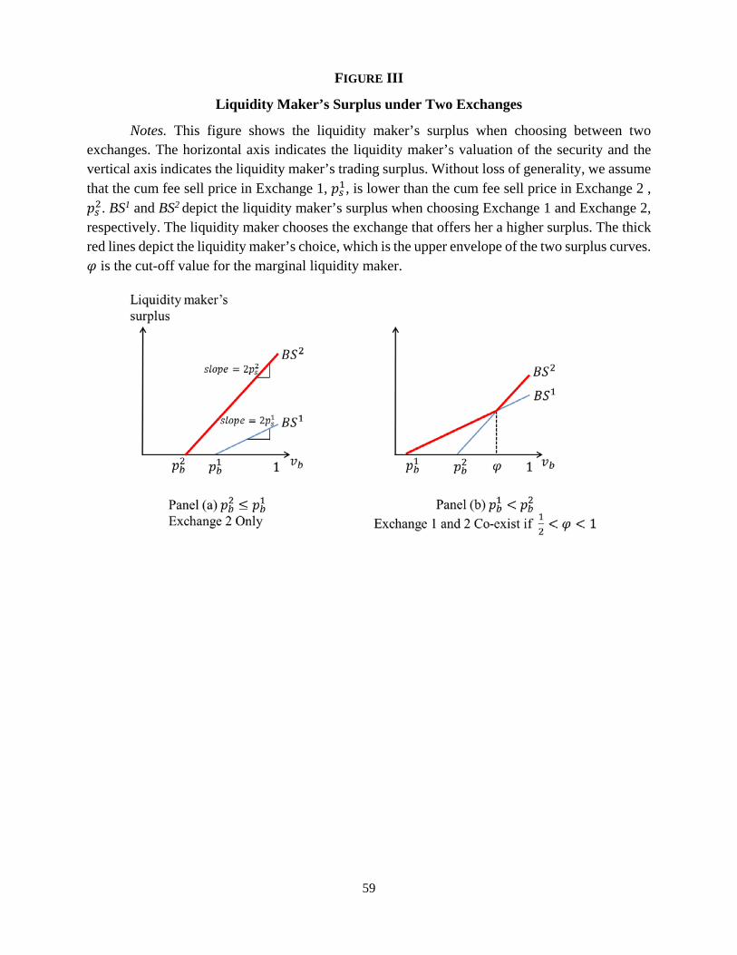
59

FIGURE III

Liquidity Maker’s Surplus under Two Exchanges

Notes. This figure shows the liquidity maker’s surplus when choosing between two exchanges. The horizontal axis indicates the liquidity maker’s valuation of the security and the vertical axis indicates the liquidity maker’s trading surplus. Without loss of generality, we assume that the cum fee sell price in Exchange 1, 𝑝𝑝𝑠𝑠1, is lower than the cum fee sell price in Exchange 2 , 𝑝𝑝𝑠𝑠2. BS1 and BS2 depict the liquidity maker’s surplus when choosing Exchange 1 and Exchange 2, respectively. The liquidity maker chooses the exchange that offers her a higher surplus. The thick red lines depict the liquidity maker’s choice, which is the upper envelope of the two surplus curves. 𝜑𝜑 is the cut-off value for the marginal liquidity maker.

60

FIGURE IV

Two Types of Deviation from Bertrand Equilibrium

Notes. This figure shows two types of profitable deviation for Exchange 2 when Exchange 1 and Exchange 2 start by setting the total fee at zero. The horizontal axis indicates the liquidity maker’s valuation of the security and the vertical axis indicates the liquidity maker’s trading surplus. BS1 and BS2 depict the liquidity maker’s surplus when choosing Exchange 1 and Exchange 2, respectively. In Panel (a), exchange 1 and exchange 2 start by setting 𝑝𝑝𝑏𝑏1 = 𝑝𝑝𝑠𝑠1 = 1

2. Exchange 2

can profitably deviate by decreasing the cum fee buy price to 𝑝𝑝𝑏𝑏2 = 12− 𝜇𝜇𝜀𝜀 and the cum fee sell

price to 𝑝𝑝𝑠𝑠2 = 12− 𝜀𝜀 . In Panel (b), Exchange 1 and Exchange 2 start by setting 𝑝𝑝𝑏𝑏1 = 𝑝𝑝𝑠𝑠1 < 1

2.

Exchange 2 can profitably deviate by increasing the cum fee buy price to 𝑝𝑝𝑏𝑏2 = 𝑝𝑝𝑏𝑏1 + 𝜀𝜀 and the cum fee sell price to 𝑝𝑝𝑠𝑠2 = 𝑝𝑝𝑠𝑠1 + 𝜇𝜇 ∙ 𝜀𝜀. 𝜀𝜀 > 0 and 0 < 𝜇𝜇 < 1 in both panels. The liquidity maker chooses the exchange that offers her a higher surplus. The thick red lines depict the segment of liquidity makers who are drawn to Exchange 2. 𝜑𝜑 is the cut-off value for the marginal liquidity maker.