what does bitcoin look like?down.aefweb.net/aefarticles/aef160211bouoiyour.pdfannals of economics...

ANNALS OF ECONOMICS AND FINANCE 16-2, 449–492 (2015)

What Does Bitcoin Look Like?

Jamal Bouoiyour

CATT, University of Pau, FranceE-mail: [email protected]

and

Refk Selmi*

ESC, University of Manouba, TunisiaE-mail: [email protected]

The paper seeks to address what Bitcoin looks like. Specifically, we at-tempt to identify the main determinants of Bitcoin price by means of rigorousevaluation through ARDL Bounds Testing method. Our findings reveal theextremely speculative behavior of Bitcoin, its partial usefulness in trade trans-actions without overlooking its dependence to the Shangai stock market andthe hash rate. There is no sign of Bitcoin being a safe haven. Taking a stepfurther, we re-investigate the focal link by accounting for the Chinese trad-ing bankruptcy. The results appear fairly robust. Bitcoin is still perceived asspeculative foolery and thus far from being a long-term promise.

Key Words: Bitcoin; Speculation; Trade transactions; Safe haven; Shangai stock

market; Hash rate; ARDL Bounds Testing approach.

JEL Classification Numbers: E5, F39, F65.

1. INTRODUCTION

In 2009, a pseudonymous hacker calling himself Satoshi Nakamoto cre-ated “Bitcoin”, the world’s first completely virtual and decentralized cur-rency. Since its creation, particular attention has been given to this emerg-ing money. In the wake of growing interest in Bitcoin, researchers begandealing with this nascent currency by revolving around multiple questions:Is it a speculative bubble? Is it a short-term hedge? Is it a safe haven?Is it a long-run promise? Is it a future currency? The fact that these

* Corresponding author.

449

1529-7373/2015

All rights of reproduction in any form reserved.

450 JAMAL BOUOIYOUR AND REFK SELMI

questions get frequently asked deeply highlights the “complexity” of thisphenomenon.

Unlike traditional fiat currencies (dollar, euro and yen), whose value isdetermined by law, Bitcoin is not convertible and not formally backed bya government or legal entity. Bitcoin operates like a free market system,since it does not rely on a central bank to issue it or a commercial bank tostore it. Instead, investors perform their business transactions themselveswithout any intermediary. The peer-to-peer network eliminates the tradebarriers and makes business easier. Every passing day, the increase in thenumber of companies which accept Bitcoin is making its perceived valuereal. Nevertheless, security concerns, the inelastic money supply coded viamathematic formula and unsustainable volatility have profoundly plaguedthis digital money.

Despite having a passionate following, this phenomenon is still difficultto be definitely tackled. Some studies suggest that Bitcoin is likely to be aspeculative trap than a future currency since there is no guarantee of repay-ment at any time (Kristoufek 2013; Yermack 2014; Bouoiyour et al. 2015).It is not yet heavily accepted as a payment system across wide marketsand does not have an underlying value derived neither from consumptionnor production process such as the precious metals including gold (Ciainet al. 2014; Glaster et al. 2014). Being a digital currency, Bitcoin is highlysensitive to cyber-attacks that may play a destabilizing role in the Bitcoinsystem (Bouoiyour et al. 2015). All these studies have attempted to answerseparately the aforementioned questions. There is only one study, to ourbest knowledge, that has tried to analyze more completely this phenomenonby assessing whether Bitcoin seems more driven by technical, financial orspeculative factors. Kristoufek (2014) has employed a wavelet coherencyapproach to gauge the interconnection between Bitcoin and its drivers oneby one (bivariate analysis) without considering additional variables thatmay have “pulling” role in explaining the Bitcoin price dynamic (multi-variate analysis). Studying the bivariate relationship may not be robustwhen some relevant explanatory variables are not included. On the onehand, these methods may lead to confusing outcomes since the occurrenceof noise cannot be heavily neglected, disrupting then the relationship in-vestigated (Aguiar-Conraria and Soares, 2011; Ng and Chan, 2012). Onthe other hand, wavelet decomposition is generally applied to assess thesignals and the periodicity that happen over time. Strictly speaking, whenwe consider only two variables, we generally fall on the problem of sim-ple regression without control variable which is unable to capture properresults with regard to the focal linkage.

To reach new insights and to find better paths on what the focal newdigital money looks like, we need further investigation while incorporatingseveral fundamentals recorded in the existing literature. Accurately, via

WHAT DOES BITCOIN LOOK LIKE? 451

an ARDL Bounds Testing approach, innovation accounting method andVEC Granger causality test, we examine the short-run and the long-runlinks between Bitcoin price and its potential drivers including investors’ at-tractiveness, exchange-trade volume, monetary Bitcoin velocity, estimatedoutput volume, hash rate, gold price and Shangai stock market. By doingso, we draw interesting findings: In the short-run, the investors attrac-tiveness, the exchange-trade ratio, the estimated output volume and theShangai index affect positively and significantly the Bitcoin price, whilethe monetary velocity, the hash rate and the gold price have no influence.In the long-run, the substantial impacts speculation, output volume andChinese stock market index observed in the short term become statisticallyinsignificant. The effect of exchange-trade ratio becomes less strong, whilethe effects of the monetary velocity and the gold price still insignificant.The hash rate explains significantly the dynamic of this new virtual cur-rency. These results appear fairly robust, since they change slightly whenincorporating the dummy variable relative to the bankruptcy of Chinesetrading company. The inclusion of oil price, Dow Jones index and a dummyvariable denoting the closing of Road Silk by FBI has led to unstable es-timates. Beyond the nuances of short-run and long-run relationships, thisresearch confirms the heavy speculative nature of Bitcoin and its partialusefulness in economic reasons without forgetting the important role thatplay the Chinese stock market and the processing power of Bitcoin networkin explaining this phenomenon. Moreover, this new digital money seemsfar from being a safe haven and a long-term promise.

The remainder of the article proceeds as follows: Section 2 presentsa brief literature survey. Section 3 describes our data and presents ourmethodological framework. Section 4 reports our main results and discussesthem. Section 5 focuses on robustness check. Section 6 concludes and offerssome policy implications that may be meaningful and fruitful for investorsand market regulators in the future.

2. BRIEF LITERATURE SURVEY

Bitcoin has engaged the attention of media and researchers, acknowledg-ing its complexity. Economists share different views regarding this nascentvirtual crypto-currency. The majority of researches on this phenomenonconsidered Bitcoin as speculative foolery rather than currency or paymentsystem due to its swelling volatility (Buchholz et al. 2012; Kristoufek 2013;Ciaian et al. 2014; Bouoiyour et al. 2015). Some others called it “evil”since it is not controlled nor by central banks nor by governments. Con-sistently, Glouderman (2014) argue that “economists scoffed at Bitcoin asmore of a financial experiment than a legitimate payment system. Someeconomists denounced it as evil, because its value is not backed by any gov-


ernment nor can it be used to make pretty things as can gold. Others showthat with no intrinsic value, Bitcoin’s rising price constituted a speculativebubble”. As we aim at rigorously analyzing what does Bitcoin look like, wegive a first insight by looking at main literature findings, evidencing howinteracts Bitcoin price with its potential determinants.

The study of Kristoufek (2014) attempts to determine whether Bitcoinis likely to be a safe haven, a speculative bubble or a business incomeby analyzing the potential sources of Bitcoin price fluctuations includingsupply-demand fundamentals, speculative and technical drivers. Waveletcoherency has been carried out to assess the linkage between the consideredvariables at distinct frequencies involved. The obtained results reveal thatthe fundamentals such as exchange-trade ratio play substantial role in lowerfrequencies. The Chinese market index seems a main driver of Bitcoinprice, while the contribution of gold price appears minor and sometimesunclear. He finds also that users’ interest or the speculative behaviors ofbusinesses play a powerful role on the dynamic of this new digital money.The interdependence between speculation and Bitcoin appears dominantat lower frequency bands. Specifically, the investors’ attractiveness drivesthe price of Bitcoin up during the explosive prices period, while it drives itdown under rapid decline period.

Gloser et al. (2014) try to address what intentions are businesses andinvestors following when moving their currency’s usage from domestic onesinto a crypto-currency like Bitcoin. By applying an Autoregressive Con-ditional Heteroskedasticity model, they show that the intention to gatheradditional information about the Bitcoin development has a deeper effecton its exchange volume. Nevertheless, the nexus between digital moneyand users’ interest seems insignificant when considering the volume withinthe Bitcoin system. These outcomes may be mainly attributed to the factthat users prefer usually to keep their Bitcoins in their exchange wallet toavoid speculation and possible cyber-attacks without any intention to usethem in economic reasons (trade transactions, for example).

More recently, Bouoiyour et al. (2015) examine whether Bitcoin is atrade transaction tool or risky investment. They analyze the causal rela-tionships between Bitcoin price and exchange-trade ratio on the one hand,and Bitcoin price and investors’ attractiveness on the other hand uncon-ditionally and conditioning upon relevant control variables including theChinese market index and the hash rate. To this end, they use an improvedfrequency domain approach-based on unconditional and conditional dataanalysis. Some differences with respect to the frequencies involved werefound, highlighting the difficulty to obtain clearer insights into this newcrypto-currency. This study confirms the speculative behavior of Bitcoinwithout overlooking its usefulness in economic reasons as trade transac-tions. They deduce that because its higher sensitivity to media and its


heavy association with speculation, Bitcoin remains an uncertain virtualasset. Therefore, if traders appreciate risky investments, serious disap-pointments may await the unwary users.

3. DATA AND METHODOLOGY

3.1. Data

The existing literature on Bitcoin price suggests potential factors thatmay affect significantly the dynamic of this virtual currency including in-vestors’ attractiveness, economic, macroeconomic and financial indicatorsand the technical drivers. For Bitcoin economy, we use two proxies whichare the exchange-trade ratio and the monetary velocity determined respec-tively through the Bitcoin days destroyed for given transactions and theestimated output volume. The global macroeconomic and financial indica-tors that may impact the evolution of Bitcoin price include the gold priceand the Shangai stock market index. Bitcoin technical drivers have beenmeasured via the hash rate. Before beginning our analysis, it seems ofutmost importance to give some details about the variables investigated:

- The Bitcoin price (BPI): The Bitcoin is new digital money that hasrecently attracted media and a wide range of people. It is an alternativecurrency to the fiat currencies including dollar, euro and yen, with severaladvantages like lower transactions fees and transparent information abouttransactions. It has also some drawbacks including the lack of legal security,the extra volatility and the great speculation (Kristoufek 2014; Bouoiyouret al. 2015).

- The investors’ attractiveness (TTR): As a proxy of investors’ attrac-tiveness to Bitcoin, we use daily Bitcoin views from Google as it able toproperly depict the speculative character of users (Kristoufek 2013). Thisindicator is determined via the frequency of the online Google search queriesrelated to the new digital money generally and Bitcoin particularly. Ar-guably, Piskorec et al. (2014) highlight the effectiveness of this proxy toaccurately describe the behavior of investors.

- The exchange-trade ratio (ETR): The trade and exchange transactionsexpand the utility of holding the currency, leading to an increase in Bitcoinprice. The exchange-trade ratio is measured as a ratio between volumes onthe currency exchange market and trade (Bouoiyour et al. 2015).

- The monetary velocity (MBV): By definition, the velocity of money isthe frequency at which one unit of each currency is used to purchase trad-able or non-tradable products for a given period. Because of the large dailyfluctuations of Bitcoin, the velocity of the economy of this new currencyhas stayed relatively stable (Kristoufek 2014).


- The estimated output volume (EOV): It is similar to the total outputvolume with the addition of an algorithm which tries to remove changefrom the total value. This may reflect more accurately the true transactionvolume. Basically, there is a negative relationship between the estimatedoutput volume and Bitcoin price. Accordingly, Kristoufek (2014) showsthat an increase in the estimated output volume leads to a drop in Bitcoinprice in the long-run.

- The Hash rate (HASH): The emergence of Bitcoin has provided newapproaches concerning payments. Hence, some new words have emergedsuch as the “hash rate”. It represents an indicator of the processing powerof the Bitcoin network. For security goal, the latter must make intensivemathematical operations, prompting an increase in the hash rate. This mayaffect widely Bitcoin purchasers and increases substantially the demand ofthis new currency and in turn their prices. Generally speaking, the hashrate is associated positively to Bitcoin price (Kristoufek 2014).

- The gold price (GP): Bitcoin does not have an underlying value derivedfrom consumption or production process such as gold. In that context,Ciaian et al. (2014) and Yermack (2014) provide evidence that there is anysign of Bitcoin being a safe haven.

- The Shangai market index (SI): The Shangai market is considered asthe biggest player in Bitcoin economy and as a result may be perceivedas a potential source of Bitcoin price volatility. Arguably, the announce-ment that Baidu (potential determinant of the Chinese online shopping)is accepting Bitcoin has affected considerably the price of the focal virtualcurrency. Recently, Bouoiyour et al. (2015), using an improved frequencydomain approach-based on unconditional vs. conditional data analysis, findthat Bitcoin is likely to be a speculative trap rather than business income,conditioning upon the performance of the Shangai market.

For empirical purpose, this study disentangles the existence of long-runcointegration between the aforementioned variables during the period span-ning between 05/12/2010 and 14/06/2014 (equation 1). Taking a step fur-ther, we re-examine the link between this nascent money and its relevantdeterminants by accounting for the Chinese trading bankruptcy. We in-clude a dummy variable that amounts 1 from 02/2013 and 0 otherwise(equation 2). All these data are extracted from Blockchain1 and quandl2.To improve the precision power of results, we carry out a log-linear speci-fication that incorporates TTR, ETR, MBV, EOV, HASH, GP and SI.

LBPIt = α0 + α1LTTRt + α2LETR+ α3LMBVt + α4LEOVt

+ α5LHASHt + α6LGPt + α7LSIt + εt (1)

1https://blockchain.info/2http://www.quandl.com/


LBPIt = β0 + β1LTTRt + β2LETR+ β3LMBVt + β4LEOVt

+ β5LHASHt + β6LGPt + β7LSIt + β8DV + ξt (2)

where ε, ξ are the error terms with normal distribution, zero mean andfinite variance. The letter L preceding the variable names indicates Log.Kristoufek (2013, 2014) and Bouoiyour et al. (2015) assume that an in-creased users’ interest searching for information about Bitcoin leads to anincrease in Bitcoin prices. Then, we expect α1, β1 > 0. The exchange-traderatio denotes the ratio between volumes on the currency exchange marketand trade. Generally, the price of the currency is positively associated tothe use of transactions as it expands the utility of holding the currency.So, it is expected that α2, β2 > 0. The monetary velocity of this money ismeasured through the number of Bitcoin in a transaction multiplied by thenumber of days where coins are already spent. Greater is Bitcoin velocity,greater will be Bitcoin prices (Ciaian et al. 2014). We expect α3, β3 > 0.An increase in the estimated output volume affects negatively Bitcoin pricein the long term (Kristoufek, 2014). We expect therefore α4, β4 < 0. Thehash rate is associated positively to Bitcoin price. An increase in Bit-coin price generates the intention of market participants to invest and tomine. We expect that α5, β5 > 0. Some studies indicate that that Bitcoincannot be perceived as safe haven since they found that there is no signifi-cant correlation between it and gold price (Kristoufek 2014). In contrast,Palombizio and Morris (2012) show that gold price may be considered asthe main source of demand and cost pressures and then seems a meaningfulcontributor of Bitcoin price dynamic. We expect α6, β6 > 0. The Shangaimarket is one of the most substantial players on digital currencies (in par-ticular, Bitcoin). We expect thus that α7, β7 > 0. The Chinese tradingbankruptcy may affect intensely Bitcoin price. Unsurprisingly, the Chinesemarket seems the Biggest Bitcoin market. So, we expect that β8 < 0.

3.2. The ARDL Bounds Testing Method

To empirically investigate the long-run relationships and dynamic in-teractions among economic variables, we can use the bounds testing (orautoregressive distributed lag: ARDL) cointegration procedure introducedby Pesaran and Shin (1999). This procedure is pursued for at least fourreasons. First, it allows us to estimate the cointegration relationship viaOLS once the lag order of the model is well identified. Second, it enables toassess simultaneously the short-run and the long-run coefficients associatedto the variables studied. Third, the bounds testing procedure does not re-quire the pre-testing of the variables included in the model for unit rootsunlike the Johansen cointegration for instance. It obviates the need to clas-


sify the time series into I(0) or I(1). Lastly, the test seems parsimonious insmall sample data as is the case in the present research. Nevertheless, theprocedure will crash in the presence of I(2) series.

The current study employs this method while attempting to rigorouslyaddress how Bitcoin looks like by examining the connection between Bitcoinprice and the aforementioned relevant variables (Equation 1). To ensurethe robustness of our results, we incorporate a dummy variable that denotesthe bankruptcy of Chinese trading company equals to 1 from 02/2013 and0 otherwise(Equation 2). The ARDL representation of equations (1) and(2) are formulated as follows:

DLBPIt = a0 +

n∑i=1

a1iDLBPIt−1 +

m∑i=0

a2iDLTTRt−1 +

l∑i=0

a3iDLETRt−1 +

h∑i=0

a4iDLMBVt−1

+

v∑i=0

a5iDLEOVt−1 +

r∑t=0

a6iDLHASHt−1 +

s∑t=0

a7iDLGPt−1 +

z∑i=0

a8iDLSIt−1

+ b1LBPIt−1 + b2LTTRt−1 + b3LETRt−1 + b4LMBVt−1 + b5LEOVt−1

+ b6LHASHt−1 + b7LGPt−1 + b8LSIt−1 + ε′t (3)

DLBPIt = c0 +

n∑i=1

c1iDLBPIt−1 +

m∑i=0

c2iDLTTRt−1 +

l∑i=0

c3iDLETRt−1 +

h∑i=0

c4iDLMBVt−1

+v∑

i=0

c5iDLEOVt−1 +

r∑t=0

c6iDLHASHt−1 +

s∑t=0

c7iDLGPt−1 +

z∑i=0

c8iDLSIt−1

+ d1LBPIt−1 + d2LTTRt−1 + d3LETRt−1 + d4LMBVt−1 + d5LEOVt−1

+ d6LHASHt−1 + d7LGPt−1 + d8LSIt−1 + d9DV + ξ′t (4)

where D denotes the first difference operator; ε′, ξ′ are the usual whitenoise residuals. To evaluate whether there is a cointegration or not de-pends upon the critical bounds tabulated by Pesaran et al. (2001, pp.300).There is a cointegration among variables if calculated F-statistic is morethan upper critical bound. If the lower bound is superior to the computedF-statistic, we accept the null hypothesis of no cointegration. Moreover, ifthe F-statistic is between lower and upper critical bounds, the cointegrationoutcomes are inconclusive. The stability of ARDL approach is assessed bycarrying out various diagnostic tests and stability analysis. The diagnos-tic tests include the adjustment R-squared, the standard error regression,Breush-Godfrey-serial correlation and Ramsey Reset test. The stabilityof short-run and long-run estimates is checked by applying the cumula-tive sum of recursive residuals, the cumulative sum of squares of recursiveresiduals and the recursive coefficients.

3.3. The innovative accounting approach and VEC Grangercausality

The majority of empirical studies use the standard Granger causality testaugmented with a lagged error correction term to analyze the causal links


between economic variables. However, this method may be ineffective sinceit is unable to properly detect the possible shocks. Given this limitation andwhile trying to avoid pitfalls, we explore an innovative accounting approachby simulating variance decomposition and impulse response function. Todo so, we decompose forecast error variance for Bitcoin price following aone standard deviation shock to investors’ attractiveness, exchange-tradevolume, monetary Bitcoin velocity, estimated output volume, hash rate,gold price and Shangai market index. Specifically, this technique enablesto effectively depict how long independent variable reacts to its own shocksand shocks stemming in the dependent variables. Moreover and in an effortto identify whether there is a short-run causality between the variablesinvestigated , the Granger causality/Block Exogeneity Wald tests basedupon VEC model may be useful. It determines if the lags of any timeseries does not Granger cause any other variable in the system using anLM test. The null hypothesis is accepted or rejected based on Wald chi-square test.

4. RESULTS AND DISCUSSION

4.1. ARDL results

To determine the most potential driver of Bitcoin price dynamic, westart by reporting the descriptive statistics (TABLE 1). We clearly showa substantial data variability, highlighting the need to use robust models.The coefficient of kurtosis appears inferior to 3 for all variables (exceptLTTR, LETR, LMBV and LEOV), indicating that the distribution is lessflattened than normal distribution. The Skewness coefficient is positive forall time series (except LETR and LGP), providing that the asymmetricaldistribution is plausible. The Jarque-Bera test revealed high and significantvalues, leading to reject the assumption of normality for all the consideredvariables.

Before proceeding ARDL estimation, we determine the degree of inte-gration of variables through Augmented Dickey-Fuller (ADF) and Phillips-Perron (PP) tests. The results are reported in TABLE 2. We clearly noticethat the variables are integrated either at level or at first difference. Thisimplies that the ARDL procedure can be followed to test the cointegrationhypothesis among the focal series.

As the lag order of the variables is an important step for the modelspecification within ARDL bounds testing framework, ., we determine thelag optimization based on lag-order selection among various informationcriteria including Akaike Information Criterion (AIC), Schwarz informationcriterion (SC) and Hannan-Quinn criterion (HQ). Since AIC has superiorpower properties for sample data compared to any lag length criterion, weshow that the optimum lag is 3 (TABLE 3).


TABLE 1.

Summary of statistics

LBPI LTTR LETR LMBV LEOV LHASH LGP LSI

Mean 3.05291 1.574058 13.41844 15.01983 13.69757 10.83858 7.319273 7.744138

Median 2.50797 1.565531 13.32571 14.95729 13.68825 9.846016 7.357317 7.717494

Maximum 7.04838 4.804185 18.09288 18.97052 17.10051 18.45453 7.547765 8.022789

Minimum −1.48069 −1.033161 4.057230 11.58991 10.64887 4.528026 7.084017 7.568131

Std. Dev. 2.07871 0.918618 2.235922 1.019057 1.033003 3.263868 0.120834 0.114295

Skewness 0.20358 0.201630 −0.668879 0.116808 0.009475 0.687444 −0.243169 0.761047

Kurtosis 2.28016 3.326236 4.017153 3.887130 3.684876 2.922190 1.703855 2.590701

Jarque-Bera 21.2311 8.362903 87.78542 26.12393 14.57141 58.86658 59.57174 77.22019

Probability 0.00002 0.015276 0.000000 0.000002 0.000685 0.000000 0.000000 0.000000

TABLE 2.

Results of ADF and PP Unit Tests

Variables ADF test PP test

Level First difference Level First difference

LBPI - −15.8916∗∗∗ - −32.5107∗∗∗

LTTR −5.8908∗∗ - −15.5010∗∗∗ -

LETR −2.9074∗∗ - −31.0877∗∗∗ -

LMBV −5.5649∗∗∗ - −25.8706∗∗∗ -

LEOV −3.7443∗∗ - - −72.5447∗∗∗

LHASH - −29.0159∗∗∗ - −13.7236∗∗∗

LGP - −26.9126∗∗∗ - −23.3523∗∗∗

LSI - −28.5842∗∗∗ - −18.5978∗∗∗

Notes: ∗∗∗, ∗∗ and ∗ imply significance at the 1%, 5% and 10% level, respectively ; Thenumbers within parentheses for the ADF and PP statistics represents the lag length ofthe dependent variable used to obtain white noise residuals ; The lag lengths for theADF and PP tests were selected using Akaike Information Criterion (AIC).

The main results obtained through ARDL Bounds testing approach arereported in TABLE 4. We worthy show that: the investors’ attractivenessplays a significant role in explaining Bitcoin price formation. Notably, anincrease by 10% in TTR expands the BTP by about 2.01%. The exchange-trade ratio affects positively and significantly the price of Bitcoin. Anincrease by 10% of ETR leads to an increase by 0.32% of BPI. Bitcoinvelocity, estimated output volume and gold price have no significant impacton Bitcoin price, while the influence of technical driver (HASH) seemspositive and significant but minor. We notice that an increase by 10% ofHASH prompts an increase by 0.03% in the prices of Bitcoin. Interestingly,


TABLE 3.

Lag-order selection

Lag LogL LR FPE AIC SC HQ

0 795.3703 NA 0.006820 −2.149987 −2.048775 −2.110926

1 799.7037 8.463462 0.006758 −2.159183 −2.051645∗ −2.117680

2 802.3041 5.071735∗ 0.006728 −2.163598 −2.049734 −2.119654∗

3 803.4872 2.304132 0.00672∗ −2.164103∗ −2.043913 −2.117718

4 803.6028 0.224915 0.006741 −2.161663 −2.035148 −2.112837

5 803.6350 0.062545 0.006759 −2.158993 −2.026152 −2.107726

6 803.9671 0.643943 0.006772 −2.157151 −2.017984 −2.103442

7 804.0653 0.190309 0.006789 −2.154663 −2.009171 −2.098513

8 804.9309 1.673839 0.006791 −2.154292 −2.002474 −2.095701

Notes: ∗ indicates lag order selected by the criterion; LR: sequential modified LR teststatistic (each test at 5% level); FPE: Final prediction error; AIC: Akaike criterion; SC:Schwarz information criterion; HQ: Hannan-Quinn information criterion.

Shangai market index contributes positively and significantly to BPI (i.e.,an increase by 10% of SI leads to an increase by 1.18% in Bitcoin price).

In addition, we depict from TABLE 5 that the value of F-statistic ex-ceeds the upper bound at the 10% significance level, implying that there isevidence of a long-run relationship among variables at this level of signifi-cance. These results seem insufficient to capture accurately the evidence oflong-term linkage because ARDL bounds test is unable to detect structuralbreaks stemming in the considered time series.

Given its inability to account for possible shocks, discontinuities andsudden disturbances, we believe that it is important to apply the methodof Gregory and Hansen (1996) to re-explore the interactions between thevariables studied while accounting for nonlinearity. This technique is basedon an unknown structural break stemming in the focal variables with re-spect to Engle-Granger residual. This test reinforces the fact that there isa long-run cointegration between Bitcoin price and its drivers even if weconsider regime shifts or structural breaks (TABLE 6).

The diagnostic tests show that there is no evidence of serial correlation.The Ramsey reset test statistic reveals the performance of the short-runmodel (TABLE 4). The CUSUM and the CUSUM Squares test show theadequacy of the considered models at 5% level of significance (FIG. 1) andthe stability of ARDL parameters (FIG. 2).

From our results reported in TABLE 7, it is well shown that Bitcoin priceinteracts differently with its determinants depending to time periods (shortor long terms). In the short-run, the users’ interest, the exchange-traderatio, the estimated output volume and the Shangai index affect positivelyand significantly the BPI. However, the monetary velocity, the hash rate


TABLE 4.

The ARDL Bounds Testing Analysis

Dependent variable: DLBPIt

C 0.6078 (1.0537)

DLBPIt−1 0.11687∗∗ (2.96916)

DLBPIt−2 0.11154∗∗ (2.95493)

DLBPIt−3 −0.0618 (−1.6440)

DLTTRt−1 0.20127∗∗∗ (9.12259)

DLETRt−1 0.0329∗ (1.6778)

DLMBVt−1 0.00134 (0.2775)

DLEOVt−1 0.0030 (0.37838)

DLHASHt−1 0.01192 (0.4814)

DLGPt−1 0.17445 (0.6631)

DLSIt−1 0.1182∗ (1.9049)

LBPIt−1 −0.01014 (−1.0310)

LTTRt−1 0.0038 (0.4752)

LETRt−1 0.0096∗ (1.8057)

LMBVt−1 0.0038 (0.6587)

LEOVt−1 0.0034 (0.5983)

LHASHt−1 0.0035∗ (1.7380)

LGPt−1 −0.1189 (−1.3637)

LSIt−1 0.02128 (0.4324)

Diagnostic tests

R-squared 0.4586

SE regression 0.8859

Breush-Godfrey serial correlation 0.0955 [0.9089]

Ramsey Reset test 0.03503 [0.8516]

Notes: ∗∗∗, ∗∗ and ∗ imply significance at the 1%, 5% and 10%level, respectively; [.]: p-value.

and the gold price have no influence on this digital money. These outcomeschange remarkably in the long-run. The TTR, the EOV and the SI whichplay the major role in the short term, have any effect on BPI in the long-run.The impact of ETR on BPI stills positive and significant, but becomes muchless important. The impacts of MBV and GP on BPI remain insignificant,while the hash rate appears as significant player. Furthermore, the valueof ECT is negative and statistically significant at 5 percent level, which istheoretically correct. Notably, the deviation in the short-run is correctedby 0.0007% towards the long-run equilibrium path. The R-squared valueindicates that 44% of Bitcoin price dynamic is explained by the explanatoryvariables.


TABLE 5.


Estimated model Optimal lag length F-statistic Prob.

FBPI (LBPI/LTTR, 3, 3,4, 1, 0, 0 4.702941∗ 0.0106

LETR, LMBV, LEOV,

LHASH, LGP, LSI)

Significance level Critical values: T = 21

Lower bounds I(0) Upper bounds I(1)

1% 6.84 7.84

5% 4.94 5.73

10% 4.04 4.78

Notes: ∗∗∗, ∗∗ and ∗ imply significance at the 1%, 5% and 10% levels,respectively; Critical values were obtained from Pesaran et al. (2001).

TABLE 6.

Gregory-Hansen Structural Break Cointegration Test

Estimated model FBPI (LBPI/LTTR, LETR, LMBV, LEOV, LHASH, LGP, LSI)

Structural break 27/10/2013

year

ADF-test −4.9861∗∗

Prob.values 0.0029

Significance level Critical values of the ADF test

1% −5.8652

5% −4.9271

10% −4.8135

Notes: ∗∗∗, ∗∗ and ∗ imply significance at the 1%, 5% and 10% level, respectively.

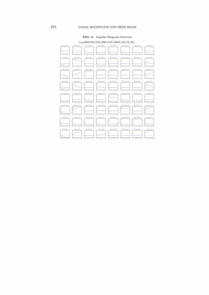
4.2. Innovative accounting approach results

The results of the variance decomposition are reported in TABLE 8. Wefind that 69.17% percent of Bitcoin price is explained by its own innovativeshocks. The investors’ attractiveness (TTR) seems the major driver ofBitcoin price (20.34%). The contribution of ETR appears minor (0.16%).Likewise, the monetary velocity, the estimated output volume and the hashrate do not have great effect on this new crypto-currency, with respectivepercentages equal to 0.035%, 0.037% and 0.003%. Gold price explainsslightly BPI (0.095%), but we should not forget that the link between GPand BPI is insignificant in the aforementioned results. Additionally, thecontribution of Chinese market index (SI) affects deeply the dynamic ofBPI (10.14%).

To be more effective in our analysis, we add the results of the impulseresponse function. It traces the time path of the impacts of shocks ofindependent variable on the dependent variables in a VAR system. By


FIG. 1. Plots of cumulative sum of recursive and of squares of recursive residuals


The diagnostic tests show that there is no evidence of serial

correlation. The Ramsey reset test statistic reveals the performance of

the short-run model (TABLE 4). The CUSUM and the CUSUM

Squares test show the adequacy of the considered models at 5% level of

significance (FIG. 2) and the stability of ARDL parameters (FIG. 3).

FIG.1.

Plots of cumulative sum of recursive and of squares of recursive residuals

-80

-60

-40

-20

0

20

40

60

80

I II III IV I II III IV

2011 2012

CUSUM 5% Significance

-0.2

0.0

0.2

0.4

0.6

0.8

1.0

1.2

IV I II III IV I II III IV

2011 2012

CUSUM of Squares 5% Significance

Notes: The straight lines represent the critical bounds at 5% significance level.


applying this technique, we can see the strength of the response of Bitcoinprice to its own shock on the one hand and those of investors’ attractiveness,exchange-trade volume, monetary velocity, estimated output volume, hashrate, gold price and Shangai market index on the other hand. FIG. 3worthy indicates that the responses in Bitcoin price owing to forecast errorstemming in TTR and SI seem positive over time, while the contributionsof ETR, MBV, EOV, HASH and GP to Bitcoin price appear negligible.

Furthermore, we evaluate whether there is a causal relationship betweenthe Bitcoin price dynamic and its aforementioned fundamentals. Beforetesting the non-causality hypothesis, we start by examining the residu-als using the LM test for serial independence against the alternative ofAR(k)/MA(k), for k = 1, . . . , 12. From the findings reported in TABLE 9,the serial correlation may be removed at the maximum lag length which is3.


FIG. 2. Plots of cumulative sum of recursive coefficients


FIG. 3.

Plots of cumulative sum of recursive coefficients

-400

-300

-200

-100

0

100

200


2011 2012

Recursive C(1) Estimates

± 2 S.E.

-2

0

2

4

6

8


2011 2012


± 2 S.E.

-3

-2

-1

0

1

2

3


2011 2012


± 2 S.E.

-3

-2

-1

0

1

2


2011 2012


± 2 S.E.

-3

-2

-1

0

1


2011 2012


± 2 S.E.

-3

-2

-1

0

1


2011 2012


± 2 S.E.

-.4

-.2

.0

.2

.4

.6


2011 2012


± 2 S.E.

-0.5

0.0

0.5

1.0

1.5

2.0


2011 2012


± 2 S.E.

-6

-4

-2

0

2

4


2011 2012


± 2 S.E.

-20

-10

0

10

20


2011 2012


± 2 S.E.

-30

-20

-10

0

10


2011 2012


± 2 S.E.

-8

-6

-4

-2

0

2


2011 2012


± 2 S.E.

-2

0

2

4

6


2011 2012


± 2 S.E.

-2

0

2

4

6


2011 2012


± 2 S.E.

-.8

-.6

-.4

-.2

.0

.2

.4


2011 2012


± 2 S.E.

-4

-3

-2

-1

0

1


2011 2012


± 2 S.E.

-2

0

2

4

6


2011 2012


± 2 S.E.

-30

-20

-10

0

10

20


2011 2012


± 2 S.E.

-20

0

20

40

60


2011 2012


± 2 S.E.


From our results reported in TABLE 7, it is well shown that Bitcoin price

interacts differently with its determinants depending to time periods (short or

long terms). In the short-run, the users’ interest, the exchange-trade ratio, the

estimated output volume and the Shangai index affect positively and

significantly the BPI. However, the monetary velocity, the hash rate and the

gold price have no influence on this digital money. These outcomes change

remarkably in the long-run. The TTR, the EOV and the SI which play the

major role in the short term, have any effect on BPI in the long-run. The

impact of ETR on BPI stills positive and significant, but becomes much less

important. The impacts of MBV and GP on BPI remain insignificant, while the


The non-causality test findings are reported in TABLE 10. It is wellnoticeable that we can reject the null hypothesis of no causality for therelationships running from DLTTR to DLBPI, DLETR to DLBPI andDLSI to DLBPI, while the reverse link is not supported for any case. Thisconfirms the above outcomes obtained through the ARDL Bounds Testingmethod and the innovation accounting approach. For the rest of variables,


FIG. 3. Impulse Response Function


FIG.4.

Impulse Response Function

-0.5

0.0

0.5

1.0

1.5

2 4 6 8 10

Response of BPI to BPI

-0.5

0.0

0.5

1.0

1.5

2 4 6 8 10

Response of BPI to TTR

-0.5

0.0

0.5

1.0

1.5

2 4 6 8 10

Response of BPI to ETR

-0.5

0.0

0.5

1.0

1.5

2 4 6 8 10

Response of BPI to MBV

-0.5

0.0

0.5

1.0

1.5

2 4 6 8 10

Response of BPI to EOV

-0.5

0.0

0.5

1.0

1.5

2 4 6 8 10

Response of BPI to HASH

-0.5

0.0

0.5

1.0

1.5

2 4 6 8 10

Response of BPI to GP

-0.5

0.0

0.5

1.0

1.5

2 4 6 8 10

Response of BPI to SI

0.0

0.5

1.0

2 4 6 8 10

Response of TTR to BPI

0.0

0.5

1.0

2 4 6 8 10

Response of TTR to TTR

0.0

0.5

1.0

2 4 6 8 10

Response of TTR to ETR

0.0

0.5

1.0

2 4 6 8 10

Response of TTR to MBV

0.0

0.5

1.0

2 4 6 8 10

Response of TTR to EOV

0.0

0.5

1.0

2 4 6 8 10

Response of TTR to HASH

0.0

0.5

1.0

2 4 6 8 10

Response of TTR to GP

0.0

0.5

1.0

2 4 6 8 10

Response of TTR to SI

-2

0

2

4

2 4 6 8 10

Response of ETR to BPI

-2

0

2

4

2 4 6 8 10

Response of ETR to TTR

-2

0

2

4

2 4 6 8 10

Response of ETR to ETR

-2

0

2

4

2 4 6 8 10

Response of ETR to MBV

-2

0

2

4

2 4 6 8 10

Response of ETR to EOV

-2

0

2

4

2 4 6 8 10

Response of ETR to HASH

-2

0

2

4

2 4 6 8 10

Response of ETR to GP

-2

0

2

4

2 4 6 8 10

Response of ETR to SI

-4

-2

0

2

2 4 6 8 10

Response of MBV to BPI

-4

-2

0

2

2 4 6 8 10

Response of MBV to TTR

-4

-2

0

2

2 4 6 8 10

Response of MBV to ETR

-4

-2

0

2

2 4 6 8 10

Response of MBV to MBV

-4

-2

0

2

2 4 6 8 10

Response of MBV to EOV

-4

-2

0

2

2 4 6 8 10

Response of MBV to HASH

-4

-2

0

2

2 4 6 8 10

Response of MBV to GP

-4

-2

0

2

2 4 6 8 10

Response of MBV to SI

-4

-2

0

2

2 4 6 8 10

Response of EOV to BPI

-4

-2

0

2

2 4 6 8 10

Response of EOV to TTR

-4

-2

0

2

2 4 6 8 10

Response of EOV to ETR

-4

-2

0

2

2 4 6 8 10

Response of EOV to MBV

-4

-2

0

2

2 4 6 8 10

Response of EOV to EOV

-4

-2

0

2

2 4 6 8 10

Response of EOV to HASH

-4

-2

0

2

2 4 6 8 10

Response of EOV to GP

-4

-2

0

2

2 4 6 8 10

Response of EOV to SI

0.0

0.5

1.0

2 4 6 8 10

Response of HASH to BPI

0.0

0.5

1.0

2 4 6 8 10

Response of HASH to TTR

0.0

0.5

1.0

2 4 6 8 10

Response of HASH to ETR

0.0

0.5

1.0

2 4 6 8 10

Response of HASH to MBV

0.0

0.5

1.0

2 4 6 8 10

Response of HASH to EOV

0.0

0.5

1.0

2 4 6 8 10

Response of HASH to HASH

0.0

0.5

1.0

2 4 6 8 10

Response of HASH to GP

0.0

0.5

1.0

2 4 6 8 10

Response of HASH to SI

-4

-2

0

2

2 4 6 8 10

Response of GP to BPI

-4

-2

0

2

2 4 6 8 10

Response of GP to TTR

-4

-2

0

2

2 4 6 8 10

Response of GP to ETR

-4

-2

0

2

2 4 6 8 10

Response of GP to MBV

-4

-2

0

2

2 4 6 8 10

Response of GP to EOV

-4

-2

0

2

2 4 6 8 10

Response of GP to HASH

-4

-2

0

2

2 4 6 8 10

Response of GP to GP

-4

-2

0

2

2 4 6 8 10

Response of GP to SI

0.0

0.5

1.0

2 4 6 8 10

Response of SI to BPI

0.0

0.5

1.0

2 4 6 8 10

Response of SI to TTR

0.0

0.5

1.0

2 4 6 8 10

Response of SI to ETR

0.0

0.5

1.0

2 4 6 8 10

Response of SI to MBV

0.0

0.5

1.0

2 4 6 8 10

Response of SI to EOV

0.0

0.5

1.0

2 4 6 8 10

Response of SI to HASH

0.0

0.5

1.0

2 4 6 8 10

Response of SI to GP

0.0

0.5

1.0

2 4 6 8 10

Response of SI to SI

Response to Nonfactorized One Unit Innovations


TABLE 7.

Short-run and long-run Analysis

Dependent variable: LBPIt

Short-run

DLBPIt 0.1252∗∗∗ (3.1873)

DLTTRt 0.5269∗∗ (2.8944)

DLETRt 0.1287∗∗∗ (7.0988)

DLMBVt 2.7411 (0.2189)

DLEOVt 0.0798∗∗∗ (3.6287)

DLHASHt 0.0594 (0.5379)

DLGPt −0.2415 (−0.9103)

DLSIt 0.3802∗ (1.6444)

ECTt −7.97E-06∗∗ (−2.5130)

Long-run

LBPIt 0.1328∗∗∗ (3.3635)

LTTRt 0.1434 (0.5414)

LETRt 0.0180∗ (1.7073)

LMBVt 0.0043 (0.8892)

LEOVt 0.0073 (0.8993)

LHASHt 0.0072∗ (1.8478)

LGPt −0.0015 (−0.1556)

LSIt 0.2157 (0.1062)

Diagnostic tests

R-squared 0.44




Notes : ∗∗∗, ∗∗ and ∗ imply significance at the 1%, 5% and10% levels, respectively Diagnostic tests results are based on F-statistic ; [.] : p-values.

we accept the null hypothesis of non-causality (except for the linkage thatruns from DLBPI to DLHASH and from DLBPI to DLMBV ). Theseresults may be very useful for investors and market regulators.

5. ROBUSTNESS

The above findings clearly indicate that although of TTR, EOV and SIcontribute greatly to the dynamic of BPI in the short-run; they appearwithout statistically significant effect in the long-run. While the monetaryvelocity, the hash rate and the gold price have no influence in the short


TABLE 8.

Variance Decomposition of Bitcoin price

Period S.E. LBPI LTTR LETR LMBV LEOV LHASH LGP LSI

1 0.089209 100.0000 0.000000 0.000000 0.000000 0.000000 0.000000 0.000000 0.000000

2 0.133356 69.62125 20.02477 0.099387 0.021195 0.048033 0.000927 0.002721 10.18171

3 0.173881 69.36913 20.14811 0.154151 0.041684 0.040414 0.008345 0.074429 10.16373

4 0.207915 69.31502 20.21095 0.143917 0.034885 0.040420 0.005948 0.079367 10.16948

5 0.237979 69.26216 20.26038 0.154534 0.037175 0.038559 0.004840 0.083554 10.15879

6 0.264822 69.22643 20.29075 0.160299 0.037687 0.038561 0.004506 0.087948 10.15380

7 0.289336 69.20724 20.31188 0.161535 0.037241 0.038131 0.003989 0.091187 10.14878

8 0.311935 69.19196 20.32765 0.163871 0.036489 0.037956 0.003689 0.093026 10.14535

9 0.333019 69.18027 20.33966 0.165645 0.035905 0.037888 0.003476 0.094519 10.14264

10 0.352847 69.17171 20.34903 0.166578 0.035233 0.037921 0.003293 0.095698 10.14054

TABLE 9.

VEC Residual Serial Correlation LM Tests

Null Hypothesis: no serial correlation at lag order h

Lags LM-Stat Prob

1 165.7815 0.0000

2 162.7223 0.0000

3 172.6073 0.0000

4 74.87208 0.1661

5 108.8017 0.0004

6 52.65505 0.8435

7 86.67175 0.0312

8 59.58174 0.6333

9 73.80962 0.1882

10 67.46570 0.3595

11 69.17378 0.3071

12 88.51908 0.0229

term. The impacts of MBV and GP on BPI seem insignificant eitherin the short or in the long-run, while the effect of the hash rate on BPIseems positive and significant in the long term. To check ensure the ro-bustness of these results, we re-estimate the relationship between Bitcoinprice and its determinants even if we incorporate a dummy variable relativeto the bankruptcy of Chinese trading company while respecting the samesteps. The accurate outcomes are reported in TABLE A-1, TABLE A-2,TABLE A-3, TABLE A-4, TABLE A-5, TABLE A-6, FIG A-1, FIG A-2and FIG A-3 (APPENDIX). Comparing these results with the previous


TABLE 10.

VEC Granger Causality/Block Exogeneity Wald Tests

Dependent variable: DLBPI

Excluded Chi-sq df Prob

DLTTR 6= DLBPI 4.4897 2 0.0474

DLBPI 6= DLTTR 0.7034 2 0.7035

DLETR 6= DLBPI 2.9722 2 0.0226

DLBPI 6= DLETR 4.2470 2 0.1196

DLMBV 6= DLBPI 0.9299 2 0.6281

DLBPI 6= DLMBV 13.698 2 0.0011

DLEOV 6= DLBPI 1.1004 2 0.5768

DLBPI 6= DLEOV 1.9394 2 0.3792

DLHASH 6= DLBPI 0.3544 2 0.8376

DLBPI 6= DLHASH 6.2336 2 0.0443

DLGP 6= DLBPI 1.0579 2 0.3574

DLBPI 6= DLGP 1.0588 2 0.3572

DLSI 6= DLBPI 3.5051 2 0.0733

DLBPI 6= DLSI 1.4394 2 0.4869

ones (i.e., without dummy variable), we put in evidence that the effects ofTTR, ETR, MBV , EOV , HASH, GP and SI are solid and unambiguous,especially with respect to time-horizons (short-and long-run). Beyond thenuances of short and long terms, the present study confirms the speculativenature of Bitcoin without overlooking its “partial” usefulness in economicreasons (trade transactions) and its great dependence to the Chinese stockmarket and the processing power of Bitcoin network. Bitcoin is thereforeperceived as speculative bubble, risky investment, short-term hedge andpartially as business income. This new crypto-currency appears far frombeing a safe haven or a long-term promise.

Further explanatory variables have been added to reach conclusive out-comes (for example, oil price3, Dow Jones index4 and a dummy variable de-

3Palombizio and Morris (2012) find that oil price (OP ) is a potential factor that mayaffect intensely inflation. If the price of oil experienced excessive ups and downs (i.e.,sizeable volatility), the Bitcoin will depreciate.

4The relationship between Bitcoin price and the Dow Jones index (DJI) appearscomplex, since the two variables seem sometimes correlated but not usually. For instance,after the announcement of American satellite TV provider that it would start acceptingBitcoin as payment tool, the prices of this digital money increased approximately by$40 touching the level of $600, while the Dow Jones Index was down by 300 points.This seems a perfect example of how the Bitcoin and the American markets have beeninitially unrelated. Nevertheless, the offshoots of Al-Qaeda over different cities in Iraqand the Obama’s declaration that America will not send the military to fight off theterrorist organizations have affected simultaneously Bitcoin and Dow Jones index. Due


noting the closing of road silk by FBI5 (DV ′) equals to one from 23/10/2013and 0 otherwise). Nevertheless, the obtained findings reveal that the effectsof the additional time series are in the majority of cases insignificant andthe estimates become clearly unstable (see FIG A-4, particularly). Moredetails about these results are summarized in TABLE A-7, TABLE A-8,TABLE A-9, TABLE A-9, TABLE A-11, TABLE A-12, FIG A-5 and FIGA-6 (APPENDIX).

6. CONCLUSIONS AND SOME POLICY IMPLICATIONS

The present research attempts to reach clearer knowledge and betterpaths into a complex phenomenon: Bitcoin price. By attempting to ad-dress what does Bitcoin looks like, several extended questions emerge: Isit a speculative bubble? Is it a short-term hedge? Is it a safe haven? Isit a long-term promise? Is it a future currency? To effectively answerthese questions, we have regressed Bitcoin price on investors’ attractive-ness, exchange-trade volume, monetary velocity, estimated output volume,hash rate, gold price and Shangai market index using an ARDL BoundsTesting method, an innovation accounting approach and VEC Grangercausality test for daily data covering the period from December 2010 toJune 2014. By doing so, we clearly show the unpleasant speculative be-havior of Bitcoin. We also provide insightful evidence that Bitcoin may beserved partially for trade transactions. However, there is any sign of beinga safe haven. By accounting for the Chinese trading bankruptcy, the con-tribution of speculation and the Shangai stock market remain dominant,while the role of Bitcoin as business income dissipates in the long-run,highlighting the robustness of our results.

So, is Bitcoin a long-term promise? Given our obtained findings, it isdifficult to reach clearer, solid and unambiguous evidence into Bitcoin phe-nomenon, since it is uncertain. This nascent digital money can remain as itcan disappear, especially when considering that Bitcoin faces a structuraleconomic problem regarding its limited amount recording 21 million unitsin 2140, implying that the money supply cannot continue to rise after thisdate. There are, up to now, 12 million Bitcoin in circulation. If this famouscrypto-currency successfully displace fiat currencies (euro, dollar and yen),it will exert sizable deflationary pressures. Without definitely tackling the

to the great connection between the turmoil and Bitcoin’s value, the price of Bitcoinstarted dropping and as response the Dow Jones index started falling by 200 points.This implies that there is some relation between both variables. For details, you canrefer to the following link: http://coinbrief.net/bitcoin-price-news-analysis/

5The Road Silk is a roating-platform of drug on which transactions were throughBitcoin. Thus, its closing by FBI in 23/10/2013 has affected substantially the dynamicof Bitcoin price.


causes, the virtual currency seems highly correlated to the speculative be-haviors of investors or people who hold it. This digital money is not issuedby banking system and even less by any government, but by a computingalgorithm. Unfortunately, the majority of users have not acknowledgedabout mathematical programs, and it is therefore unknown for them howfar it can go. In sum, no one can predict the precise value and the spe-cific form crypto-urrency will take since the technological development isheavily unpredictable. As technology becomes increasingly integrated intoour everyday lives, crypto-currencies will obviously continue to grow andBitcoin may probably be displaced by better digital currencies.

Intuitively, the sizeable volatility of Bitcoin and the difficulty of process-ing power network are likely to discourage investors. Additionally, the greatattention to this crypto-currency in the Chinese media has drawn a hugenumber of Bitcoin believers in Chinese market. However, the ambiguousattitude of regulators towards Bitcoin in China, coupled with the typicalChinese investor’s lack of experience will prompt an intensive speculation(Mei et al. 2009). This reinforces the evidence that this new virtual cur-rency is likely to be short-term hedge and risky investment rather thanlong-term promise. There is a greater chance that Bitcoin collapses anddisappears tomorrow rather than suddenly become internationally recog-nized.

REFERENCES

Aguiar-Conraria, Luis and Maria-Joana Soares, 2011. The continuous wavelet trans-form: A primer. NIPE working paper no.16, University of Minho.

Bouoiyour, Jamal, Refk Selmi, and Aviral-Kumar Tiwari, 2015. Is Bitcoin business in-come or speculative foolery? New ideas through an improved frequency domain anal-ysis. Annals of Financial Economics 10(1), 1-23. DOI: 10.1142/S2010495215500025

Breitung, Jorg and Bertrand Candelon, 2006. Testing for short and long-run causality:a frequency domain approach. Journal of Econometrics 132, 363-378.

Buchholz, Martis, Jess Delaney, Joseph Warren, and Jeff Parker, 2012. Bits and Bets,Information, Price Volatility, and Demand for Bitcoin. Economics 312.

Ciaian, Pavel, Miroslava Rajcaniova, and d’Artis Kancs, 2014. The Economics ofBitCoin Price Formation. http://arxiv.org/ftp/arxiv/papers/1405/1405.4498.pdf

Glaster, Florian, Zimmermann Kai, Martin Haferkorn, and Mortiz Weber, 2014.Bitcoin-asset or currency? Revealing users’ hidden intentions, Twenty Second Eu-ropean Conference on Information Systems.

Glouderman, Laren, 2014. Bitcoin’s Uncertain Future in China. USCC EconomicIssue Brief 4, May 12.

Gregory, Allan and Bruce Hansen, 1996. Residual based Tests for Co-integration inModels with Regime Shifts. Journal of Econometrics 70, 99-126.

Kristoufek, Ladislav, 2013. BitCoin meets Google Trends and Wikipedia: Quantifyingthe relationship between phenomena of the Internet era. Scientific Reports 3 (3415),1-7.


Kristoufek, Ladislav, 2014. What are the main drivers of the Bitcoin price? Evidencefrom wavelet coherence analysis. http://arxiv.org/pdf/1406.0268.pdf

Mei, Jianping, Jose A. Scheinkman, and Wei Xiong, 2009. Speculative Trading andStock Prices: Evidence from Chinese A-B Share Premia. Annals of Economics andFinance 10(2), 225-255.

Ng, Eric and Johnny Chan, 2012. Geophysical Applications of Partial WaveletCoherence and Multiple Wavelet Coherence. American Meteological Society. DOI:10.1175/JTECH-D-12-00056.1

Palombizio, Ennio and Ian Morris, 2012. Forecasting Exchange Rates using LeadingEconomic Indicators. Open Access Scientific Reports 1(8), 1-6.

Pesaran, M. and Y. Shin, 1999. An Autoregressive Distributed Lag Modeling Ap-proach to Cointegration Analysis. S. Strom, (ed) Econometrics and Economic Theoryin the 20th Century, Cambridge University.

Pesaran, Hashem, Yongcheol Shin, and Richard Smith, 2001. Bounds testing ap-proaches to the analysis of level relationships. Journal of Applied Econometrics 16,289-326.

Piskorec, Matija, Antulov-Fantulin Nino, Novak Petra, Mozetic Igor, Gricar Miha,Vodenska Irena, and Smuc Tomislav, 2014. News Cohesiveness: an Indicator of Sys-temic Risk in Financial Markets. http://arxiv.org/pdf/1402.3483v1.pdf

Yermack, David, 2013. Is Bitcoin a Real Currency? An economic appraisal. NBER-WP no. 19747. http://www.nber.org/papers/w19747


APPENDIX A

TABLE 1.

Lag-order selection


FBPI (LBPI/LTTR, LETR, LMBV, LEOV, LHASH, LGP, LSI, DV)

0 781.6729 NA 0.007309 −2.080742 −1.974351∗ −2.039709∗

1 782.5517 1.714736 0.007312 −2.080413 −1.967763 −2.036966

2 782.9059 0.690066 0.007325 −2.078656 −1.959747 −2.032795

3 785.3696 4.793244∗ 0.007295∗ −2.082638∗ −1.957472 −2.034364

4 785.3825 0.025151 0.007315 −2.079952 −1.948528 −2.029264

5 785.4114 0.056055 0.007334 −2.077310 −1.939627 −2.024208

6 785.4309 0.037764 0.007354 −2.074642 −1.930700 −2.019126

7 785.4515 0.039790 0.007374 −2.071977 −1.921777 −2.014047

8 785.6675 0.417417 0.007390 −2.069844 −1.913385 −2.009500

Notes: ∗ indicates lag order selected by the criterion; LR: sequential modified LR test statistic(each test at 5% level); FPE: Final prediction error; AIC: Akaike information criterion; SC:Schwarz information criterion; HQ: Hannan-Quinn information criterion; DV: denotes thebankruptcy of Chinese trading company equals to 1 from 02/2013 and 0 otherwise.


TABLE 2.


Dependent variable: DLBPIt

C 3.4815 (1.1373)

DLBPIt−1 0.5641∗∗ (3.0184)

DLBPIt−2 0.1557∗∗∗ (3.8357)

DLTTRt−1 0.4846∗ (1.8352)

DLETRt−1 0.0825∗ (1.6934)

DLMBVt−1 0.0049 (0.2057)

DLEOVt−1 0.0428 (1.9022)

DLHASHt−1 0.0075 (0.4132)

DLGPt−1 0.3248 (0.1847)

DLSIt−1 0.3516∗ (2.2567)

LBPIt−1 0.1602∗∗∗ (3.2488)

LTTRt−1 0.0336 (1.1308)

LETRt−1 0.0314 (0.8947)

LMBVt−1 0.0344 (1.2216)

LEOVt−1 0.0137 (0.4755)

LHASHt−1 0.0092∗ (1.8607)

LGPt−1 −0.0555 (−1.1431)

LSIt−1 −1.0622 (−0.8250)

DV −0.0957 (−1.8796)

R-squared 0.48




Notes: ∗∗∗, ∗∗ and ∗ imply significance at the 1%, 5% and10% level, respectively; DV : denotes the bankruptcy of Chi-nese trading company equals to 1 from 02/2013 and 0 oth-erwise; [.]: p-value.


TABLE 3.



FBPI (LBPI/LTTR, LETR, 3, 3,4, 1, 0, 0 4.2852∗ 0.0381

LMBV, LEOV, LHASH, LGP,

LSI, DV)

Significance level Critical values


1% 6.84 7.84

5% 4.94 5.73

10% 4.04 4.78

Notes: ∗∗∗, ∗∗ and ∗ imply significance at the 1%, 5% and 10% levels, respec-tively; Critical values were obtained from Pesaran et al. (2001); DV: denotes thebankruptcy of Chinese trading company equals to 1 from 02/2013 and 0 otherwise.

TABLE 4.

Gregory-Hansen Structural Break Cointegration Test

Estimated model FBPI (LBPI/LTTR, LETR, LMBV, LEOV, LHASH, LGP, LSI, DV)

Structural break year 18/12/2013

ADF-test −4.8743∗∗∗

Prob. values 0.0000


1% −5.8652

5% −4.9271

10% −4.8135

Notes: ∗∗∗, ∗∗ and ∗ imply significance at the 1%, 5% and 10% level, respectively; DV: denotes thebankruptcy of Chinese trading company equals to 1 from 02/2013 and 0 otherwise.


FIG. 1. Plots of cumulative sum of recursive and of squares of recursive residuals


FIG. A-1.

Plots of cumulative sum of recursive and of squares of recursive residuals


-80

-60

-40

-20

0

20

40

60

80


2012 2013


-0.2

0.0

0.2

0.4

0.6

0.8

1.0

1.2


2012 2013


Notes: The straight lines represent the critical bounds at 5% significance level; DV: denotes the

bankruptcy of Chinese trading company equals to 1 from 02/2013 and 0 otherwise.

Notes: The straight lines represent the critical bounds at 5% significance level;

DV : denotes the bankruptcy of Chinese trading company equals to 1 from

02/2013 and 0 otherwise.


FIG. 2. Plots of cumulative sum of recursive coefficients


FIG. A-2.

Plots of cumulative sum of recursive coefficients

FBPI (LBPI/LTTR, LETR, LMBV, LEOV, LHASH, LGP, LGP, LSI, DV)

-5

0

5

10

15

20

M4 M5 M6 M7 M8 M9 M10 M11 M12

2013


± 2 S.E.

-1.2

-0.8

-0.4

0.0

0.4

M4 M5 M6 M7 M8 M9 M10 M11 M12

2013


± 2 S.E.

-.25

-.20

-.15

-.10

-.05

.00

.05

M4 M5 M6 M7 M8 M9 M10 M11 M12

2013


± 2 S.E.

-.12

-.08

-.04

.00

.04

.08

M4 M5 M6 M7 M8 M9 M10 M11 M12

2013


± 2 S.E.

-4

-2

0

2

4

M4 M5 M6 M7 M8 M9 M10 M11 M12

2013


± 2 S.E.

-.4

-.2

.0

.2

.4

.6

.8

M4 M5 M6 M7 M8 M9 M10 M11 M12

2013


± 2 S.E.

-.05

.00

.05

.10

M4 M5 M6 M7 M8 M9 M10 M11 M12

2013


± 2 S.E.

-.05

.00

.05

.10

.15

.20

M4 M5 M6 M7 M8 M9 M10 M11 M12

2013


± 2 S.E.

-.2

.0

.2

.4

.6

.8

M4 M5 M6 M7 M8 M9 M10 M11 M12

2013


± 2 S.E.

-0.4

0.0

0.4

0.8

1.2

M4 M5 M6 M7 M8 M9 M10 M11 M12

2013


± 2 S.E.

-6

-4

-2

0

2

4

M4 M5 M6 M7 M8 M9 M10 M11 M12

2013


± 2 S.E.

-.3

-.2

-.1

.0

.1

M4 M5 M6 M7 M8 M9 M10 M11 M12

2013


± 2 S.E.

-3

-2

-1

0

1

M4 M5 M6 M7 M8 M9 M10 M11 M12

2013


± 2 S.E.

-.3

-.2

-.1

.0

.1

M4 M5 M6 M7 M8 M9 M10 M11 M12

2013


± 2 S.E.

-.10

-.05

.00

.05

.10

.15

M4 M5 M6 M7 M8 M9 M10 M11 M12

2013


± 2 S.E.

-.10

-.05

.00

.05

.10

M4 M5 M6 M7 M8 M9 M10 M11 M12

2013


± 2 S.E.

-.1

.0

.1

.2

.3

.4

M4 M5 M6 M7 M8 M9 M10 M11 M12

2013


± 2 S.E.

-.3

-.2

-.1

.0

.1

M4 M5 M6 M7 M8 M9 M10 M11 M12

2013


± 2 S.E.

-1.2

-0.8

-0.4

0.0

0.4

0.8

M4 M5 M6 M7 M8 M9 M10 M11 M12

2013


± 2 S.E.

-.3

-.2

-.1

.0

.1

.2

.3

M4 M5 M6 M7 M8 M9 M10 M11 M12

2013


± 2 S.E. Notes: The straight lines represent the critical bounds at 5% significance level; DV: denotes the bankruptcy of

Chinese trading company equals to 1 from 02/2013 and 0 otherwise.


DV: denotes the bankruptcy of Chinese trading company equals to 1 from 02/2013

and 0 otherwise.


TABLE 5.

Short-run and long-run Analysis


Short-run

DLBPIt 0.3722∗∗∗ (7.6306)

DLTTRt 0.3107∗∗ (3.2019)

DLETRt 0.0954∗∗∗ (5.4125)

DLMBVt −5.1072 (−1.3082)

DLEOVt 0.1583∗∗∗ (3.7943)

DLHASHt 0.3040 (0.1569)

DLGPt −0.0238 (−0.9867)

DLSIt 0.2272∗∗ (2.9769)

ECTt −3.20E-06∗ (−1.7186)

Long-run

LBPIt 0.2309∗∗∗ (4.7347)

LTTRt 0.0279 (1.2933)

LETRt 0.0222∗ (1.9182)

LMBVt 0.0287 (0.9623)

LEOVt −0.0030 (−0.0778)

LHASHt 0.0076∗ (1.9784)

LGPt 0.2140 (0.8852)

LSIt 0.3295 (0.2478)

DV −0.0812∗ (−1.7697)

R-squared 0.36




Notes : ∗∗∗, ∗∗ and ∗ imply significance at the 1%, 5% and10% levels, respectively Diagnostic tests results are based onF-statistic ; DV : denotes the bankruptcy of Chinese tradingcompany equals to 1 from 02/2013 and 0 otherwise; [.] : p-values.


TABLE 6.



1 0.437211 100.0000 0.000000 0.000000 0.000000 0.000000 0.000000 0.000000 0.000000

2 0.531016 69.16401 20.07857 0.046293 0.192572 0.172621 0.216206 7.05E-05 10.12964

3 0.587408 68.89641 20.06423 0.074224 0.207786 0.157107 0.180322 0.175893 10.24402

4 0.653719 68.88240 20.05204 0.094030 0.169006 0.140286 0.155463 0.211353 10.29542

5 0.713412 68.85767 20.04848 0.091867 0.142428 0.156410 0.158901 0.212927 10.33130

6 0.765985 68.85128 20.04238 0.094067 0.123555 0.162226 0.144646 0.224575 10.35726

7 0.815668 68.84969 20.03788 0.097420 0.109980 0.162901 0.135923 0.233969 10.37223

8 0.862787 68.84846 20.03494 0.099140 0.098834 0.165991 0.130940 0.239833 10.38186

9 0.907295 68.84839 20.03210 0.100438 0.090140 0.169011 0.125686 0.244983 10.38925

10 0.949679 68.84880 20.02980 0.101707 0.083155 0.170850 0.121426 0.249415 10.39483


FIG. 3. Impulse Response Function


TABLE A-6.



1 0.437211 100.0000 0.000000 0.000000 0.000000 0.000000 0.000000 0.000000 0.000000

2 0.531016 69.16401 20.07857 0.046293 0.192572 0.172621 0.216206 7.05E-05 10.12964

3 0.587408 68.89641 20.06423 0.074224 0.207786 0.157107 0.180322 0.175893 10.24402

4 0.653719 68.88240 20.05204 0.094030 0.169006 0.140286 0.155463 0.211353 10.29542

5 0.713412 68.85767 20.04848 0.091867 0.142428 0.156410 0.158901 0.212927 10.33130

6 0.765985 68.85128 20.04238 0.094067 0.123555 0.162226 0.144646 0.224575 10.35726

7 0.815668 68.84969 20.03788 0.097420 0.109980 0.162901 0.135923 0.233969 10.37223

8 0.862787 68.84846 20.03494 0.099140 0.098834 0.165991 0.130940 0.239833 10.38186

9 0.907295 68.84839 20.03210 0.100438 0.090140 0.169011 0.125686 0.244983 10.38925

10 0.949679 68.84880 20.02980 0.101707 0.083155 0.170850 0.121426 0.249415 10.39483

FIG. A-3.

Impulse Response Function


-.2

.0

.2

.4

.6

2 4 6 8 10


-.2

.0

.2

.4

.6

2 4 6 8 10


-.2

.0

.2

.4

.6

2 4 6 8 10


-.2

.0

.2

.4

.6

2 4 6 8 10


-.2

.0

.2

.4

.6

2 4 6 8 10


-.2

.0

.2

.4

.6

2 4 6 8 10


-.2

.0

.2

.4

.6

2 4 6 8 10


-.2

.0

.2

.4

.6

2 4 6 8 10


-.4

.0

.4

.8

2 4 6 8 10


-.4

.0

.4

.8

2 4 6 8 10


-.4

.0

.4

.8

2 4 6 8 10


-.4

.0

.4

.8

2 4 6 8 10


-.4

.0

.4

.8

2 4 6 8 10


-.4

.0

.4

.8

2 4 6 8 10


-.4

.0

.4

.8

2 4 6 8 10


-.4

.0

.4

.8

2 4 6 8 10


-.01

.00

.01

2 4 6 8 10


-.01

.00

.01

2 4 6 8 10


-.01

.00

.01

2 4 6 8 10


-.01

.00

.01

2 4 6 8 10


-.01

.00

.01

2 4 6 8 10


-.01

.00

.01

2 4 6 8 10


-.01

.00

.01

2 4 6 8 10


-.01

.00

.01

2 4 6 8 10


-0.5

0.0

0.5

1.0

2 4 6 8 10


-0.5

0.0

0.5

1.0

2 4 6 8 10


-0.5

0.0

0.5

1.0

2 4 6 8 10


-0.5

0.0

0.5

1.0

2 4 6 8 10


-0.5

0.0

0.5

1.0

2 4 6 8 10


-0.5

0.0

0.5

1.0

2 4 6 8 10


-0.5

0.0

0.5

1.0

2 4 6 8 10


-0.5

0.0

0.5

1.0

2 4 6 8 10


-.2

.0

.2

.4

.6

2 4 6 8 10


-.2

.0

.2

.4

.6

2 4 6 8 10


-.2

.0

.2

.4

.6

2 4 6 8 10


-.2

.0

.2

.4

.6

2 4 6 8 10


-.2

.0

.2

.4

.6

2 4 6 8 10


-.2

.0

.2

.4

.6

2 4 6 8 10


-.2

.0

.2

.4

.6

2 4 6 8 10


-.2

.0

.2

.4

.6

2 4 6 8 10


-.08

-.04

.00

.04

.08

.12

2 4 6 8 10


-.08

-.04

.00

.04

.08

.12

2 4 6 8 10


-.08

-.04

.00

.04

.08

.12

2 4 6 8 10


-.08

-.04

.00

.04

.08

.12

2 4 6 8 10


-.08

-.04

.00

.04

.08

.12

2 4 6 8 10


-.08

-.04

.00

.04

.08

.12

2 4 6 8 10


-.08

-.04

.00

.04

.08

.12

2 4 6 8 10


-.08

-.04

.00

.04

.08

.12

2 4 6 8 10


-.005

.000

.005

.010

.015

2 4 6 8 10


-.005

.000

.005

.010

.015

2 4 6 8 10


-.005

.000

.005

.010

.015

2 4 6 8 10


-.005

.000

.005

.010

.015

2 4 6 8 10


-.005

.000

.005

.010

.015

2 4 6 8 10


-.005

.000

.005

.010

.015

2 4 6 8 10


-.005

.000

.005

.010

.015

2 4 6 8 10


-.005

.000

.005

.010

.015

2 4 6 8 10


-0.5

0.0

0.5

1.0

2 4 6 8 10


-0.5

0.0

0.5

1.0

2 4 6 8 10


-0.5

0.0

0.5

1.0

2 4 6 8 10


-0.5

0.0

0.5

1.0

2 4 6 8 10


-0.5

0.0

0.5

1.0

2 4 6 8 10


-0.5

0.0

0.5

1.0

2 4 6 8 10


-0.5

0.0

0.5

1.0

2 4 6 8 10


-0.5

0.0

0.5

1.0

2 4 6 8 10


Response to Nonfactorized One S.D. Innovations


TABLE 7.

Lag-order selection (Equations with additional variables)


(1) : FBPI (LBPI/LTTR, LETR, LMBV, LEOV, LHASH, LGP, LOP, LDJI, LSI)

0 3678.627 NA∗ 2.36e-06∗ −10.11759∗ −10.04801∗ −10.09074∗

1 3678.644 0.032814 2.37e-06 −10.11488 −10.03897 −10.08558

2 3678.673 0.057395 2.38e-06 −10.11220 −10.02997 −10.08046

3 3678.675 0.003638 2.38e-06 −10.10945 −10.02089 −10.07527

(2) : FBPI (LBPI/LTTR, LETR, LMBV, LEOV, LHASH, LGP, LOP, LDJI, LSI, DV)

0 782.4109 NA 0.006972 −2.128030 −2.058447 −2.101176

1 788.0603 11.11191 0.006883 −2.140856 −2.064947∗ −2.111560∗

2 791.0228 5.818642 0.006846 −2.146270∗ −2.064035 −2.114533

3 792.0847 2.082820 0.006844∗ −2.146441 −2.05738 −2.112262

(3) : FBPI (LBPI/LTTR, LETR, LMBV, LEOV, LHASH, LGP, LOP, LDJI, LSI, DV ′)

0 163.4746 NA 0.004414 −2.585117 −2.544254 −2.569759

1 164.5226 20.77749 0.004348 −2.600201∗ −2.555252∗ −2.583308

2 164.5759 1.055509 0.004351 −2.599458 −2.550422 −2.581029∗

3 164.6161 0.795628 0.004355∗ −2.598506 −2.545384 −2.578541

Notes: ∗ indicates lag order selected by the criterion; LR: sequential modified LR test statis-tic (each test at 5% level); FPE: Final prediction error; AIC: Akaike information criterion;SC: Schwarz information criterion; HQ: Hannan-Quinn information criterion. DV: denotes thebankruptcy of Chinese trading company equals to 1 from 02/2013 and 0 otherwise; DV’: corre-sponds to the closing of the Road Silk by FBI, which amounts 1 from 23/10/2013 and 0 otherwise.


TABLE 8.

The ARDL Bounds Testing Analysis (Equations with additional variables)

Dependent variable: ∆LBPIt

(1) (2) (3)

C −2.4325∗ −1.7262∗ −1.4941∗

(−1.7278) (−2.5645) (−2.1939)

∆LBPIt−1 0.1185∗∗ 0.0376∗ 0.0288∗

(3.0231) (2.0056) (1.6232)

∆LBPIt−2 - 0.0394∗ -

(2.2019)

∆LTTRt−1 0.1222∗∗ 0.2062∗ 0.0068∗

(3.1537) (1.7683) (1.7044)

∆LETRt−1 0.1153∗∗ 0.0093∗ 0.0087∗

(3.0589) (1.8553) (1.7147)

∆LMBVt−1 −0.1222 0.0010 0.0011

(−0.2482) (0.4548) (0.6971)

∆LEOVt−1 0.0030 0.0016 0.0021

(0.3763) (0.4187) (0.5425)

∆LHASHt−1 −0.0141 −0.0079 −0.0060

(−0.5719) (−0.6775) (−0.5051)

∆LGPt−1 0.1559 −0.0614 −0.1064

(0.5900) (−0.4894) (−0.8379)

∆LOPt−1 −0.1043 0.1004 0.0086

(−0.5383) (1.0901) (0.9297)

∆LDJIt−1 −0.1268 −0.1267 −0.0971

(−0.3857) (−0.8120) (−0.6185)

∆LSIt−1 0.1468∗ 0.1235∗ 0.1104∗

(2.000) (1.9516) (1.8452)

LBPIt−1 0.0186∗ 0.0141∗∗ −0.0079

(1.6551) (2.6353) (−1.3922)

LTTRt−1 −0.0162 0.0043 −0.0064

(−1.5979) (1.0714) (−1.3244)

LETRt−1 0.0158∗ 0.0039∗ 0.0059∗

(2.2800) (1.9519) (1.8516)

LMBVt−1 0.0032 −0.0027 −0.0037

(0.5693) (−0.9879) (−1.3088)


TABLE 8—Continued


(1) (2) (3)

LEOVt−1 0.0026 0.0051∗ 0.0039

(0.4453) (1.7506) (1.3735)

LHASHt−1 0.0056∗ −0.0010 0.0081∗∗

(1.8862) (−0.5489) (2.6473)

LGPt−1 −0.0534 −0.0011 −0.0143

(−0.9023) (−0.0405) (−0.4907)

LOPt−1 −0.0161 −0.0653 −0.0310

(−0.2627) (−0.2364) (−0.9948)

LDJIt−1 0.0355∗ 0.1008∗∗∗ 0.1002∗∗∗

(2.2728) (3.8895) (4.0147)

LSIt−1 0.0762 0.0104 −0.0186

(1.3060) (0.3766) (−0.5807)

DV - −0.0163∗ -

(−1.7604)

DV ′ - - −0.0278∗

(−2.4188)

R-squared 0.54 0.44 0.42

SE regression 0.8881 0.7923 0.7795

Breush-Godfrey 0.6231 [0.4097] 0.0069 [0.9338] 0.0081 [0.4276]

serial correlation

Ramsey Reset test 0.2664 [0.6058] 0.0316 [0.9689] 0.0049 [0.6618]

Notes: ∗∗∗, ∗∗ and ∗ imply significance at the 1%, 5% and 10% level, respec-tively; [.]: p-value; DV : denotes the bankruptcy of Chinese trading companyequals to 1 from 02/2013 and 0 otherwise; DV ′: corresponds to the closing ofthe Road Silk by FBI, which amounts 1 from 23/10/2013 and 0 otherwise.


TABLE 9.

The ARDL Bounds Testing Analysis (Equations with additional variables)


(1): FBPI (LBPI/LTTR, LETR, LMBV, LEOV, 3, 3,4, 1, 0, 0, 0, 0 4.5711∗ 0.0659

LHASH, LGP, LOP, LDJI, LSI)


LHASH, LGP, LOP, LDJI, LSI, DV)


LHASH, LGP, LOP, LDJI, LSI, DV ′)

Significance level Critical values


1% 6.84 7.84

5% 4.94 5.73

10% 4.04 4.78

Notes: ∗∗∗, ∗∗ and ∗ imply significance at the 1%, 5% and 10% levels, respectively; Critical valueswere obtained from Pesaran et al. (2001); DV : denotes the bankruptcy of Chinese trading companyequals to 1 from 02/2013 and 0 otherwise; DV ′: corresponds to the closing of the Road Silk by FBI,which amounts 1 from 23/10/2013 and 0 otherwise.

TABLE 10.

Gregory-Hansen Structural Break Cointegration Test (Equations withadditional variables)

Estimated model (1): FBPI (LBPI/LTTR, (2): FBPI (LBPI/LTTR, (3): FBPI (LBPI/LTTR,

LETR, LMBV, LEOV, LETR, LMBV, LEOV, LETR, LMBV, LEOV,

LHASH, LGP, LOP, LHASH, LGP, LOP, LHASH, LGP, LOP,

LDJI, LSI) LDJI, LSI, DV) LDJI, LSI, DV)

Structural break year 23/10/2013 26/2/2013 23/10/2013

ADF-test −5.9234∗∗∗ −4.9782∗∗ −5.2139∗∗∗

Prob.values 0.0015 0.0015 0.0004


1% −5.8652

5% −4.9271

10% −4.8135

Notes: ∗∗∗, ∗∗ and ∗ imply significance at the 1%, 5% and 10% level, respectively; DV : denotes the bankruptcy ofChinese trading company equals to 1 from 02/2013 and 0 otherwise; DV ′: corresponds to the closing of the RoadSilk by FBI, which amounts 1 from 23/10/2013 and 0 otherwise.


FIG. 4. Plots of cumulative sum of recursive and of squares of recursive residuals(Equations with additional variables)

(1):FBPI(LBPI/LTTR,LETR,LMBV,LEOV,LHASH,LGP,LOP,LDJI, LSI)


FIG A-4.

Plots of cumulative sum of recursive and of squares of recursive residuals (Equations

with additional variables)

(1): FBPI (LBPI/LTTR, LETR, LMBV, LEOV, LHASH, LGP, LOP, LDJI, LSI)

-80

-60

-40

-20

0

20

40

60

80

100 200 300 400 500 600 700


-0.2

0.0

0.2

0.4

0.6

0.8

1.0

1.2

100 200 300 400 500 600 700


(2): FBPI (LBPI/LTTR, LETR, LMBV, LEOV, LHASH, LGP, LOP, LDJI, LSI, DV)

-80

-60

-40

-20

0

20

40

60

80

100 200 300 400 500 600 700


(3): FBPI (LBPI/LTTR, LETR, LMBV, LEOV, LHASH, LGP, LOP, LDJI, LSI, DV’)


bankruptcy of Chinese trading company equals to 1 from 02/2013 and 0 otherwise; DV’:

corresponds to the closing of the Road Silk by FBI, which amounts 1 from 23/10/2013 and 0

otherwise.

-0.2

0.0

0.2

0.4

0.6

0.8

1.0

1.2

475 500 525 550 575 600 625 650 675 700 725


-40

-30

-20

-10

0

10

20

30

40

625 650 675 700 725


-0.2

0.0

0.2

0.4

0.6

0.8

1.0

1.2

625 650 675 700 725


(2):FBPI(LBPI/LTTR,LETR,LMBV,LEOV,LHASH,LGP,LOP,LDJI, LSI,DV )


FIG A-4.




-80

-60

-40

-20

0

20

40

60

80

100 200 300 400 500 600 700


-0.2

0.0

0.2

0.4

0.6

0.8

1.0

1.2

100 200 300 400 500 600 700



-80

-60

-40

-20

0

20

40

60

80

100 200 300 400 500 600 700






otherwise.

-0.2

0.0

0.2

0.4

0.6

0.8

1.0

1.2

475 500 525 550 575 600 625 650 675 700 725


-40

-30

-20

-10

0

10

20

30

40

625 650 675 700 725


-0.2

0.0

0.2

0.4

0.6

0.8

1.0

1.2

625 650 675 700 725


(3):FBPI(LBPI/LTTR,LETR,LMBV,LEOV,LHASH,LGP,LOP,LDJI, LSI,DV ′)


FIG A-4.




-80

-60

-40

-20

0

20

40

60

80

100 200 300 400 500 600 700


-0.2

0.0

0.2

0.4

0.6

0.8

1.0

1.2

100 200 300 400 500 600 700



-80

-60

-40

-20

0

20

40

60

80

100 200 300 400 500 600 700






otherwise.

-0.2

0.0

0.2

0.4

0.6

0.8

1.0

1.2

475 500 525 550 575 600 625 650 675 700 725


-40

-30

-20

-10

0

10

20

30

40

625 650 675 700 725


-0.2

0.0

0.2

0.4

0.6

0.8

1.0

1.2

625 650 675 700 725



DV : denotes the bankruptcy of Chinese trading company equals to 1 from

02/2013 and 0 otherwise; DV ′: corresponds to the closing of the Road Silk

by FBI, which amounts 1 from 23/10/2013 and 0 otherwise.


FIG. 5. Plots of cumulative sum of recursive coefficients (Equations with additionalvariables)



FIG. A-5.

Plots of cumulative sum of recursive coefficients (Equations with additional variables)


-500

0

500

1,000

1,500

100 200 300 400 500 600 700


± 2 S.E.

-3

-2

-1

0

1

2

3

100 200 300 400 500 600 700


± 2 S.E.

-3

-2

-1

0

1

2

3

100 200 300 400 500 600 700


± 2 S.E.

-4

-2

0

2

4

100 200 300 400 500 600 700


± 2 S.E.

-.2

.0

.2

.4

.6

100 200 300 400 500 600 700


± 2 S.E.

-.4

-.2

.0

.2

.4

.6

.8

100 200 300 400 500 600 700


± 2 S.E.

-6

-4

-2

0

2

100 200 300 400 500 600 700


± 2 S.E.

-10

-5

0

5

10

15

20

100 200 300 400 500 600 700


± 2 S.E.

-20

-10

0

10

20

30

40

100 200 300 400 500 600 700


± 2 S.E.

-40

-20

0

20

40

60

80

100 200 300 400 500 600 700


± 2 S.E.

-8

-4

0

4

8

12

100 200 300 400 500 600 700


± 2 S.E.

-4

-2

0

2

4

100 200 300 400 500 600 700


± 2 S.E.

-4

-2

0

2

4

100 200 300 400 500 600 700


± 2 S.E.

-2

0

2

4

6

100 200 300 400 500 600 700


± 2 S.E.

-.6

-.4

-.2

.0

.2

.4

.6

100 200 300 400 500 600 700


± 2 S.E.

-1.5

-1.0

-0.5

0.0

0.5

100 200 300 400 500 600 700


± 2 S.E.

-1

0

1

2

3

4

100 200 300 400 500 600 700


± 2 S.E.

-20

-10

0

10

100 200 300 400 500 600 700


± 2 S.E.

-80

-60

-40

-20

0

20

40

100 200 300 400 500 600 700


± 2 S.E.

-120

-80

-40

0

40

100 200 300 400 500 600 700


± 2 S.E.

-60

-40

-20

0

20

40

100 200 300 400 500 600 700


± 2 S.E.





-8

-4

0

4

8

500 550 600 650 700


± 2 S.E.

-.2

-.1

.0

.1

.2

.3

500 550 600 650 700


± 2 S.E.

.00

.05

.10

.15

.20

.25

.30

500 550 600 650 700


± 2 S.E.

-.3

-.2

-.1

.0

.1

500 550 600 650 700


± 2 S.E.

-.04

-.02

.00

.02

.04

500 550 600 650 700


± 2 S.E.

-.04

-.02

.00

.02

.04

.06

500 550 600 650 700


± 2 S.E.

-.02

-.01

.00

.01

.02

500 550 600 650 700


± 2 S.E.

-.03

-.02

-.01

.00

.01

.02

.03

500 550 600 650 700


± 2 S.E.

-.12

-.08

-.04

.00

.04

.08

500 550 600 650 700


± 2 S.E.

-1.0

-0.5

0.0

0.5

1.0

500 550 600 650 700


± 2 S.E.

-.8

-.4

.0

.4

.8

500 550 600 650 700


± 2 S.E.

-1.0

-0.5

0.0

0.5

1.0

1.5

500 550 600 650 700


± 2 S.E.

-0.5

0.0

0.5

1.0

1.5

500 550 600 650 700


± 2 S.E.

-.06

-.04

-.02

.00

.02

.04

.06

500 550 600 650 700


± 2 S.E.

-.02

-.01

.00

.01

.02

.03

500 550 600 650 700


± 2 S.E.

-.04

-.02

.00

.02

.04

500 550 600 650 700


± 2 S.E.

-.03

-.02

-.01

.00

.01

.02

500 550 600 650 700


± 2 S.E.

-.02

-.01

.00

.01

.02

500 550 600 650 700


± 2 S.E.

-.06

-.04

-.02

.00

.02

.04

500 550 600 650 700


± 2 S.E.

-.4

-.2

.0

.2

.4

500 550 600 650 700


± 2 S.E.

-.2

-.1

.0

.1

.2

.3

.4

500 550 600 650 700


± 2 S.E.

-.4

-.2

.0

.2

.4

.6

500 550 600 650 700


± 2 S.E.

-.4

-.2

.0

.2

.4

500 550 600 650 700


± 2 S.E.

-.04

.00

.04

.08

.12

500 550 600 650 700


± 2 S.E.





Notes: The straight lines represent the critical bounds at 5% significance level; DV’: The

closing of the Road Silk by FBI, which amounts 1 from 23/10/2013 and 0 otherwise.

-6

-4

-2

0

2

650 675 700 725


± 2 S.E.

.00

.05

.10

.15

.20

.25

650 675 700 725


± 2 S.E.

-.02

-.01

.00

.01

.02

.03

650 675 700 725


± 2 S.E.

-.03

-.02

-.01

.00

.01

.02

.03

650 675 700 725


± 2 S.E.

-.015

-.010

-.005

.000

.005

.010

.015

650 675 700 725


± 2 S.E.

-.02

-.01

.00

.01

.02

.03

650 675 700 725


± 2 S.E.

-.08

-.04

.00

.04

.08

650 675 700 725


± 2 S.E.

-.8

-.4

.0

.4

.8

650 675 700 725


± 2 S.E.

-.6

-.4

-.2

.0

.2

.4

650 675 700 725


± 2 S.E.

-1.2

-0.8

-0.4

0.0

0.4

0.8

650 675 700 725


± 2 S.E.

-0.4

0.0

0.4

0.8

1.2

1.6

650 675 700 725


± 2 S.E.

-.04

-.02

.00

.02

.04

650 675 700 725


± 2 S.E.

-.02

-.01

.00

.01

.02

.03

650 675 700 725


± 2 S.E.

-.02

-.01

.00

.01

.02

.03

650 675 700 725


± 2 S.E.

-.02

-.01

.00

.01

.02

650 675 700 725


± 2 S.E.

-.02

-.01

.00

.01

.02

650 675 700 725


± 2 S.E.

-.03

-.02

-.01

.00

.01

.02

650 675 700 725


± 2 S.E.

-.2

-.1

.0

.1

.2

650 675 700 725


± 2 S.E.

-.2

-.1

.0

.1

.2

650 675 700 725


± 2 S.E.

-.1

.0

.1

.2

.3

.4

.5

650 675 700 725


± 2 S.E.

-.2

-.1

.0

.1

.2

650 675 700 725


± 2 S.E.

-.04

.00

.04

.08

.12

.16

650 675 700 725


± 2 S.E.


DV’: The closing of the Road Silk by FBI, which amounts 1 from 23/10/2013

and 0 otherwise.


TABLE 11.

Short-run and long-run Analysis (Equations with additional variables)


(1) (2) (3)

Short-run

∆LBPIt 0.1270∗∗∗ 0.0281∗ 0.0269∗∗

(3.2270) (2.1537) (2.5852)

∆LTTRt 0.4305∗ 0.5702∗ 0.4787∗∗∗

(2.0214) (2.1522) (4.1026)

∆LETRt 0.2157∗∗∗ 0.0192∗∗∗ 0.0172∗∗

(8.4441) (7.3397) (2.6367)

∆LMBVt −2.2467 0.7897 0.4398∗

(−0.1721) (0.2109) (1.7485)

∆LEOVt 0.4158∗ −0.4434 0.0172

(2.5803) (−0.2068) (0.3859)

∆LHASHt −0.0283 −0.0915 −0.0057

(−0.3214) (−0.7780) (−0.3802)

∆LGPt −3.4273 −0.0054 −0.0928

(−1.5320) (−0.3213) (−0.6674)

∆LOPt −2.4806 −0.7780 0.7488

(−1.5448) (−1.4343) (1.4354)

∆LDJIt 2.0697 0.8341 −0.0259

(0.5522) (0.6264) (−1.3648)

∆LSIt 0.3256∗ 0.4786∗∗ 0.4784∗∗∗

(1.6625) (2.6372) (4.6666)

ECTt −0.0023∗∗ −0.0020∗ −0.0026∗∗

(−2.8790) (−1.6791) (−2.5190)

Long-run

LBPIt 0.1340∗∗∗ 0.1265∗∗∗ 0.1275∗∗

(3.3768) (3.2112) (3.2394)

LTTRt −0.0131 0.0016 −0.0529

(−1.3168) (0.1611) (−0.2708)

LETRt 0.0088∗ 0.0010∗ 0.0029∗

(1.8163) (1.7842) (1.8604)

LMBVt 0.0001∗∗∗ 0.0921 −0.0012

(8.8192) (0.9284) (−0.2067)


TABLE 11—Continued


(1) (2) (3)

LEOVt 0.0043 0.0655 −0.0070

(0.5435) (1.0307) (−0.8598)

LHASHt 0.0077∗ 0.0029∗ 0.0053∗

(1.9745) (1.8148) (1.8371)

LGPt 0.1518 0.1534 −0.1684

(0.5697) (0.5752) (−0.6232)

LOPt −0.0518 −0.0515 0.0019

(−0.2658) (−0.2642) (0.1915)

LDJIt 0.1420∗∗∗ 0.1852∗ 0.2417∗∗∗

(4.2680) (2.4937) (3.8358)

LSIt 0.4400 0.4406 0.4457

(1.5950) (1.5948) (1.5960)

DV - −0.0569∗ -

(−1.8245)

DV ′ - - −0.0782∗∗

(−2.2516)

R-squared 0.48 0.49 0.46

SE regression 0.8561 0.8934 0.8357

Breush-Godfrey 0.4597 [0.1386] 0.0437 [0.6795] 0.0398 [0.5012]

serial correlation

Ramsey Reset test 0.2392 [0.5674] 0.0087 [0.9015] 0.0127 [0.8564]

Notes : ∗∗∗, ∗∗ and ∗ imply significance at the 1%, 5% and 10% levels, re-spectively Diagnostic tests results are based on F-statistic ; [.] : p-values; DV :denotes the bankruptcy of Chinese trading company equals to 1 from 02/2013and 0 otherwise; DV ′: The closing of the Road Silk by FBI, which amounts 1from 23/10/2013 and 0 otherwise.


TABLE 12.

Variance Decomposition of Bitcoin price (Equations with additional variables)

Period S.E. BPI TTR ETR MBV EOV HASH GP OP DJI SI

(1): FBPI(LBPI/LTTR,LETR,LMBV,LEOV,LHASH,LGP,LOP,LDJI, LSI)

1 0.089236 100.0000 0.000000 0.00000 0.00000 0.00000 0.00000 0.000000 0.00000 0.00000 0.000000

2 0.13351 69.6429 20.1029 0.0126 0.01414 0.04282 0.00242 0.00791 0.00015 0.02165 10.1522

3 0.17424 69.3178 20.0936 0.08429 0.06908 0.08224 0.00857 0.00469 0.08981 0.13229 10.11750

4 0.20822 69.2186 20.0780 0.08772 0.06310 0.09189 0.00613 0.00385 0.13053 0.19427 10.12585

5 0.2382 69.1321 20.0764 0.09382 0.06899 0.09809 0.00475 0.00446 0.15369 0.24247 10.12509

6 0.26511 69.0742 20.0754 0.09889 0.06991 0.10429 0.00426 0.00488 0.17124 0.27213 10.12463

7 0.28958 69.0401 20.0728 0.10204 0.07004 0.10790 0.00369 0.00522 0.18245 0.2922 10.1233

8 0.31214 69.0143 20.0715 0.10456 0.06969 0.11054 0.00331 0.00547 0.19044 0.30723 10.12275

9 0.33319 68.9942 20.07075 0.10661 0.06934 0.11262 0.00304 0.00565 0.19688 0.31870 10.12211

10 0.35298 68.9790 20.06981 0.10810 0.06882 0.11434 0.00282 0.00578 0.20197 0.32762 10.12165

(2): FBPI(LBPI/LTTR,LETR,LMBV,LEOV,LHASH,LGP,LOP,LDJI, LSI,DV )

1 0.088898 100.0000 0.000000 0.000000 0.000000 0.000000 0.000000 0.000000 0.000000 0.000000 0.000000

2 0.133945 72.56927 20.13121 0.041758 8.8E-05 0.098224 0.02756 0.001589 0.000687 0.002292 17.127313

3 0.17576 72.0822 20.13425 0.14806 0.03469 0.24463 0.01796 0.08172 0.12257 0.03177 17.10206

4 0.20805 71.7392 20.10767 0.28919 0.03440 0.38193 0.02936 0.12379 0.14477 0.07531 17.07429

5 0.23777 71.1985 20.21750 0.32258 0.03296 0.64717 0.02293 0.12715 0.13963 0.21534 17.07614

6 0.26395 70.9037 20.29078 0.33606 0.04648 0.70942 0.01902 0.136528 0.17212 0.31687 17.06890

7 0.28824 70.7084 20.36059 0.33356 0.07918 0.73016 0.01595 0.137717 0.184304 0.375281 17.07481

8 0.31087 70.5771 20.40122 0.33026 0.12008 0.72251 0.01399 0.144631 0.194569 0.419226 17.07634

9 0.33261 70.4270 20.44057 0.34394 0.16216 0.72334 0.01347 0.146085 0.200372 0.461578 17.08140

10 0.35326 70.2972 20.48197 0.35034 0.20136 0.72406 0.01223 0.149376 0.210477 0.488857 17.08410

(3): FBPI(LBPI/LTTR,LETR,LMBV,LEOV,LHASH,LGP,LOP,LDJI, LSI,DV ′)

1 0.087395 100.0000 0.000000 0.000000 0.000000 0.000000 0.000000 0.000000 0.000000 0.000000 0.000000

2 0.130853 74.35845 25.00083 0.169084 0.063336 0.249291 0.056673 5.73E-05 0.015324 0.003965 10.08298

3 0.170888 74.07583 25.08213 0.210320 0.151004 0.260412 0.067889 0.071403 0.009058 0.013847 10.05810

4 0.200639 73.91041 25.06713 0.208223 0.140833 0.232576 0.149281 0.114483 0.080100 0.046427 10.05053

5 0.228146 73.36040 25.05225 0.334346 0.171296 0.384731 0.198527 0.116988 0.070455 0.209062 10.10193

6 0.251440 72.85983 25.05138 0.483718 0.211823 0.461448 0.248267 0.096316 0.075465 0.401673 10.11008

7 0.272403 72.41273 25.07048 0.585694 0.414078 0.473728 0.263102 0.097604 0.065593 0.506023 10.11096

8 0.292613 71.84532 25.11079 0.536605 0.866225 0.467039 0.267483 0.109727 0.058930 0.607852 10.13001

9 0.312471 71.23209 25.16030 0.483560 1.349822 0.463842 0.254317 0.124232 0.055452 0.733107 10.14327

10 0.332569 70.60522 25.19070 0.429863 1.850939 0.469308 0.239178 0.156563 0.053518 0.849822 10.15488

Notes: DV : denotes the bankruptcy of Chinese trading company equals to 1 from 02/2013 and 0 otherwise; DV ′:The closing of the Road Silk by FBI, which amounts 1 from 23/10/2013 and 0 otherwise.


FIG. 6. Impulse Response Functions



FIG. A-6.

Impulse Response Functions


-0 .5

0 .0

0 .5

1 .0

1 .5

2 4 6 8 10


-0 .5

0 .0

0 .5

1 .0

1 .5

2 4 6 8 10


-0 .5

0 .0

0 .5

1 .0

1 .5

2 4 6 8 10


-0 .5

0 .0

0 .5

1 .0

1 .5

2 4 6 8 10


-0 .5

0 .0

0 .5

1 .0

1 .5

2 4 6 8 10


-0 .5

0 .0

0 .5

1 .0

1 .5

2 4 6 8 10


-0 .5

0 .0

0 .5

1 .0

1 .5

2 4 6 8 10


-0 .5

0 .0

0 .5

1 .0

1 .5

2 4 6 8 10

Response of BPI to OP

-0 .5

0 .0

0 .5

1 .0

1 .5

2 4 6 8 10

Response of BPI to DJI

-0 .5

0 .0

0 .5

1 .0

1 .5

2 4 6 8 10


0 .0

0 .5

1 .0

2 4 6 8 10


0 .0

0 .5

1 .0

2 4 6 8 10


0 .0

0 .5

1 .0

2 4 6 8 10


0 .0

0 .5

1 .0

2 4 6 8 10


0 .0

0 .5

1 .0

2 4 6 8 10


0 .0

0 .5

1 .0

2 4 6 8 10


0 .0

0 .5

1 .0

2 4 6 8 10


0 .0

0 .5

1 .0

2 4 6 8 10

Response of TTR to OP

0 .0

0 .5

1 .0

2 4 6 8 10

Response of TTR to DJI

0 .0

0 .5

1 .0

2 4 6 8 10


-2

0

2

4

2 4 6 8 10


-2

0

2

4

2 4 6 8 10


-2

0

2

4

2 4 6 8 10


-2

0

2

4

2 4 6 8 10


-2

0

2

4

2 4 6 8 10


-2

0

2

4

2 4 6 8 10


-2

0

2

4

2 4 6 8 10


-2

0

2

4

2 4 6 8 10

Response of ETR to OP

-2

0

2

4

2 4 6 8 10

Response of ETR to DJI

-2

0

2

4

2 4 6 8 10


-4

-2

0

2

4

2 4 6 8 10


-4

-2

0

2

4

2 4 6 8 10


-4

-2

0

2

4

2 4 6 8 10


-4

-2

0

2

4

2 4 6 8 10


-4

-2

0

2

4

2 4 6 8 10


-4

-2

0

2

4

2 4 6 8 10


-4

-2

0

2

4

2 4 6 8 10


-4

-2

0

2

4

2 4 6 8 10

Response of MBV to OP

-4

-2

0

2

4

2 4 6 8 10

Response of MBV to DJI

-4

-2

0

2

4

2 4 6 8 10


-4

-2

0

2

4

2 4 6 8 10


-4

-2

0

2

4

2 4 6 8 10


-4

-2

0

2

4

2 4 6 8 10


-4

-2

0

2

4

2 4 6 8 10


-4

-2

0

2

4

2 4 6 8 10


-4

-2

0

2

4

2 4 6 8 10


-4

-2

0

2

4

2 4 6 8 10


-4

-2

0

2

4

2 4 6 8 10

Response of EOV to OP

-4

-2

0

2

4

2 4 6 8 10

Response of EOV to DJI

-4

-2

0

2

4

2 4 6 8 10


0 .0

0 .5

1 .0

2 4 6 8 10


0 .0

0 .5

1 .0

2 4 6 8 10


0 .0

0 .5

1 .0

2 4 6 8 10


0 .0

0 .5

1 .0

2 4 6 8 10


0 .0

0 .5

1 .0

2 4 6 8 10


0 .0

0 .5

1 .0

2 4 6 8 10


0 .0

0 .5

1 .0

2 4 6 8 10


0 .0

0 .5

1 .0

2 4 6 8 10

Response of HASH to OP

0 .0

0 .5

1 .0

2 4 6 8 10

Response of HASH to DJI

0 .0

0 .5

1 .0

2 4 6 8 10


-6

-4

-2

0

2

2 4 6 8 10


-6

-4

-2

0

2

2 4 6 8 10


-6

-4

-2

0

2

2 4 6 8 10


-6

-4

-2

0

2

2 4 6 8 10


-6

-4

-2

0

2

2 4 6 8 10


-6

-4

-2

0

2

2 4 6 8 10


-6

-4

-2

0

2

2 4 6 8 10


-6

-4

-2

0

2

2 4 6 8 10

Response of GP to OP

-6

-4

-2

0

2

2 4 6 8 10

Response of GP to DJI

-6

-4

-2

0

2

2 4 6 8 10


-0 .5

0 .0

0 .5

1 .0

1 .5

2 4 6 8 10

Response of OP to BPI

-0 .5

0 .0

0 .5

1 .0

1 .5

2 4 6 8 10

Response of OP to TTR

-0 .5

0 .0

0 .5

1 .0

1 .5

2 4 6 8 10

Response of OP to ETR

-0 .5

0 .0

0 .5

1 .0

1 .5

2 4 6 8 10

Response of OP to MBV

-0 .5

0 .0

0 .5

1 .0

1 .5

2 4 6 8 10

Response of OP to EOV

-0 .5

0 .0

0 .5

1 .0

1 .5

2 4 6 8 10

Response of OP to HASH

-0 .5

0 .0

0 .5

1 .0

1 .5

2 4 6 8 10

Response of OP to GP

-0 .5

0 .0

0 .5

1 .0

1 .5

2 4 6 8 10

Response of OP to OP

-0 .5

0 .0

0 .5

1 .0

1 .5

2 4 6 8 10

Response of OP to DJI

-0 .5

0 .0

0 .5

1 .0

1 .5

2 4 6 8 10

Response of OP to SI

0 .0

0 .5

1 .0

2 4 6 8 10

Response of DJI to BPI

0 .0

0 .5

1 .0

2 4 6 8 10

Response of DJI to TTR

0 .0

0 .5

1 .0

2 4 6 8 10

Response of DJI to ETR

0 .0

0 .5

1 .0

2 4 6 8 10

Response of DJI to MBV

0 .0

0 .5

1 .0

2 4 6 8 10

Response of DJI to EOV

0 .0

0 .5

1 .0

2 4 6 8 10

Response of DJ I to HASH

0 .0

0 .5

1 .0

2 4 6 8 10

Response of DJI to GP

0 .0

0 .5

1 .0

2 4 6 8 10

Response of DJI to OP

0 .0

0 .5

1 .0

2 4 6 8 10

Response of DJI to DJI

0 .0

0 .5

1 .0

2 4 6 8 10

Response of DJI to SI

0 .0

0 .5

1 .0

2 4 6 8 10


0 .0

0 .5

1 .0

2 4 6 8 10


0 .0

0 .5

1 .0

2 4 6 8 10


0 .0

0 .5

1 .0

2 4 6 8 10


0 .0

0 .5

1 .0

2 4 6 8 10


0 .0

0 .5

1 .0

2 4 6 8 10


0 .0

0 .5

1 .0

2 4 6 8 10


0 .0

0 .5

1 .0

2 4 6 8 10

Response of SI to OP

0 .0

0 .5

1 .0

2 4 6 8 10

Response of SI to DJI

0 .0

0 .5

1 .0

2 4 6 8 10







-0 .5

0 .0

0 .5

1 .0

1 .5

2 4 6 8 10


-0 .5

0 .0

0 .5

1 .0

1 .5

2 4 6 8 10


-0 .5

0 .0

0 .5

1 .0

1 .5

2 4 6 8 10


-0 .5

0 .0

0 .5

1 .0

1 .5

2 4 6 8 10


-0 .5

0 .0

0 .5

1 .0

1 .5

2 4 6 8 10


-0 .5

0 .0

0 .5

1 .0

1 .5

2 4 6 8 10


-0 .5

0 .0

0 .5

1 .0

1 .5

2 4 6 8 10


-0 .5

0 .0

0 .5

1 .0

1 .5

2 4 6 8 10


-0 .5

0 .0

0 .5

1 .0

1 .5

2 4 6 8 10


-0 .5

0 .0

0 .5

1 .0

1 .5

2 4 6 8 10


-0 .5

0 .0

0 .5

1 .0

1 .5

2 4 6 8 10


-0 .5

0 .0

0 .5

1 .0

1 .5

2 4 6 8 10


-0 .5

0 .0

0 .5

1 .0

1 .5

2 4 6 8 10


-0 .5

0 .0

0 .5

1 .0

1 .5

2 4 6 8 10


-0 .5

0 .0

0 .5

1 .0

1 .5

2 4 6 8 10


-0 .5

0 .0

0 .5

1 .0

1 .5

2 4 6 8 10


-0 .5

0 .0

0 .5

1 .0

1 .5

2 4 6 8 10


-0 .5

0 .0

0 .5

1 .0

1 .5

2 4 6 8 10


-0 .5

0 .0

0 .5

1 .0

1 .5

2 4 6 8 10


-0 .5

0 .0

0 .5

1 .0

1 .5

2 4 6 8 10


-2

0

2

4

6

2 4 6 8 10


-2

0

2

4

6

2 4 6 8 10


-2

0

2

4

6

2 4 6 8 10


-2

0

2

4

6

2 4 6 8 10


-2

0

2

4

6

2 4 6 8 10


-2

0

2

4

6

2 4 6 8 10


-2

0

2

4

6

2 4 6 8 10


-2

0

2

4

6

2 4 6 8 10


-2

0

2

4

6

2 4 6 8 10


-2

0

2

4

6

2 4 6 8 10


-4

0

4

2 4 6 8 10


-4

0

4

2 4 6 8 10


-4

0

4

2 4 6 8 10


-4

0

4

2 4 6 8 10


-4

0

4

2 4 6 8 10


-4

0

4

2 4 6 8 10


-4

0

4

2 4 6 8 10


-4

0

4

2 4 6 8 10


-4

0

4

2 4 6 8 10


-4

0

4

2 4 6 8 10


-4

-2

0

2

2 4 6 8 10


-4

-2

0

2

2 4 6 8 10


-4

-2

0

2

2 4 6 8 10


-4

-2

0

2

2 4 6 8 10


-4

-2

0

2

2 4 6 8 10


-4

-2

0

2

2 4 6 8 10


-4

-2

0

2

2 4 6 8 10


-4

-2

0

2

2 4 6 8 10


-4

-2

0

2

2 4 6 8 10


-4

-2

0

2

2 4 6 8 10


-0 .5

0 .0

0 .5

1 .0

2 4 6 8 10


-0 .5

0 .0

0 .5

1 .0

2 4 6 8 10


-0 .5

0 .0

0 .5

1 .0

2 4 6 8 10


-0 .5

0 .0

0 .5

1 .0

2 4 6 8 10


-0 .5

0 .0

0 .5

1 .0

2 4 6 8 10


-0 .5

0 .0

0 .5

1 .0

2 4 6 8 10

Res pons e of HASH to HASH

-0 .5

0 .0

0 .5

1 .0

2 4 6 8 10


-0 .5

0 .0

0 .5

1 .0

2 4 6 8 10


-0 .5

0 .0

0 .5

1 .0

2 4 6 8 10


-0 .5

0 .0

0 .5

1 .0

2 4 6 8 10


-0 .5

0 .0

0 .5

1 .0

1 .5

2 4 6 8 10


-0 .5

0 .0

0 .5

1 .0

1 .5

2 4 6 8 10


-0 .5

0 .0

0 .5

1 .0

1 .5

2 4 6 8 10


-0 .5

0 .0

0 .5

1 .0

1 .5

2 4 6 8 10


-0 .5

0 .0

0 .5

1 .0

1 .5

2 4 6 8 10


-0 .5

0 .0

0 .5

1 .0

1 .5

2 4 6 8 10


-0 .5

0 .0

0 .5

1 .0

1 .5

2 4 6 8 10


-0 .5

0 .0

0 .5

1 .0

1 .5

2 4 6 8 10


-0 .5

0 .0

0 .5

1 .0

1 .5

2 4 6 8 10


-0 .5

0 .0

0 .5

1 .0

1 .5

2 4 6 8 10


-8

-4

0

4

2 4 6 8 10


-8

-4

0

4

2 4 6 8 10


-8

-4

0

4

2 4 6 8 10


-8

-4

0

4

2 4 6 8 10


-8

-4

0

4

2 4 6 8 10


-8

-4

0

4

2 4 6 8 10


-8

-4

0

4

2 4 6 8 10


-8

-4

0

4

2 4 6 8 10


-8

-4

0

4

2 4 6 8 10


-8

-4

0

4

2 4 6 8 10


0 .0

0 .5

1 .0

2 4 6 8 10


0 .0

0 .5

1 .0

2 4 6 8 10


0 .0

0 .5

1 .0

2 4 6 8 10


0 .0

0 .5

1 .0

2 4 6 8 10


0 .0

0 .5

1 .0

2 4 6 8 10


0 .0

0 .5

1 .0

2 4 6 8 10

Response of DJI to HASH

0 .0

0 .5

1 .0

2 4 6 8 10


0 .0

0 .5

1 .0

2 4 6 8 10


0 .0

0 .5

1 .0

2 4 6 8 10


0 .0

0 .5

1 .0

2 4 6 8 10


0 .0

0 .5

1 .0

2 4 6 8 10


0 .0

0 .5

1 .0

2 4 6 8 10


0 .0

0 .5

1 .0

2 4 6 8 10


0 .0

0 .5

1 .0

2 4 6 8 10


0 .0

0 .5

1 .0

2 4 6 8 10


0 .0

0 .5

1 .0

2 4 6 8 10


0 .0

0 .5

1 .0

2 4 6 8 10


0 .0

0 .5

1 .0

2 4 6 8 10


0 .0

0 .5

1 .0

2 4 6 8 10


0 .0

0 .5

1 .0

2 4 6 8 10







-1

0

1

2

2 4 6 8 10


-1

0

1

2

2 4 6 8 10


-1

0

1

2

2 4 6 8 10


-1

0

1

2

2 4 6 8 10


-1

0

1

2

2 4 6 8 10


-1

0

1

2

2 4 6 8 10


-1

0

1

2

2 4 6 8 10


-1

0

1

2

2 4 6 8 10


-1

0

1

2

2 4 6 8 10


-1

0

1

2

2 4 6 8 10


-1

0

1

2

2 4 6 8 10

Response of BPI to DV2

-0 .5

0 .0

0 .5

1 .0

1 .5

2 4 6 8 10


-0 .5

0 .0

0 .5

1 .0

1 .5

2 4 6 8 10


-0 .5

0 .0

0 .5

1 .0

1 .5

2 4 6 8 10


-0 .5

0 .0

0 .5

1 .0

1 .5

2 4 6 8 10


-0 .5

0 .0

0 .5

1 .0

1 .5

2 4 6 8 10


-0 .5

0 .0

0 .5

1 .0

1 .5

2 4 6 8 10


-0 .5

0 .0

0 .5

1 .0

1 .5

2 4 6 8 10


-0 .5

0 .0

0 .5

1 .0

1 .5

2 4 6 8 10


-0 .5

0 .0

0 .5

1 .0

1 .5

2 4 6 8 10


-0 .5

0 .0

0 .5

1 .0

1 .5

2 4 6 8 10


-0 .5

0 .0

0 .5

1 .0

1 .5

2 4 6 8 10

Response of TTR to DV2

-4

0

4

8

2 4 6 8 10


-4

0

4

8

2 4 6 8 10


-4

0

4

8

2 4 6 8 10


-4

0

4

8

2 4 6 8 10


-4

0

4

8

2 4 6 8 10


-4

0

4

8

2 4 6 8 10


-4

0

4

8

2 4 6 8 10


-4

0

4

8

2 4 6 8 10


-4

0

4

8

2 4 6 8 10


-4

0

4

8

2 4 6 8 10


-4

0

4

8

2 4 6 8 10

Response of ETR to DV2

-1 0

-5

0

5

2 4 6 8 10


-1 0

-5

0

5

2 4 6 8 10


-1 0

-5

0

5

2 4 6 8 10


-1 0

-5

0

5

2 4 6 8 10


-1 0

-5

0

5

2 4 6 8 10


-1 0

-5

0

5

2 4 6 8 10


-1 0

-5

0

5

2 4 6 8 10


-1 0

-5

0

5

2 4 6 8 10


-1 0

-5

0

5

2 4 6 8 10


-1 0

-5

0

5

2 4 6 8 10


-1 0

-5

0

5

2 4 6 8 10

Response of MBV to DV2

-6

-4

-2

0

2

2 4 6 8 10


-6

-4

-2

0

2

2 4 6 8 10


-6

-4

-2

0

2

2 4 6 8 10


-6

-4

-2

0

2

2 4 6 8 10


-6

-4

-2

0

2

2 4 6 8 10


-6

-4

-2

0

2

2 4 6 8 10


-6

-4

-2

0

2

2 4 6 8 10


-6

-4

-2

0

2

2 4 6 8 10


-6

-4

-2

0

2

2 4 6 8 10


-6

-4

-2

0

2

2 4 6 8 10


-6

-4

-2

0

2

2 4 6 8 10

Response of EOV to DV2

-0 .5

0 .0

0 .5

1 .0

2 4 6 8 10


-0 .5

0 .0

0 .5

1 .0

2 4 6 8 10


-0 .5

0 .0

0 .5

1 .0

2 4 6 8 10


-0 .5

0 .0

0 .5

1 .0

2 4 6 8 10


-0 .5

0 .0

0 .5

1 .0

2 4 6 8 10


-0 .5

0 .0

0 .5

1 .0

2 4 6 8 10


-0 .5

0 .0

0 .5

1 .0

2 4 6 8 10


-0 .5

0 .0

0 .5

1 .0

2 4 6 8 10


-0 .5

0 .0

0 .5

1 .0

2 4 6 8 10


-0 .5

0 .0

0 .5

1 .0

2 4 6 8 10


-0 .5

0 .0

0 .5

1 .0

2 4 6 8 10

Response of HASH to DV2

-0 .5

0 .0

0 .5

1 .0

1 .5

2 4 6 8 10


-0 .5

0 .0

0 .5

1 .0

1 .5

2 4 6 8 10


-0 .5

0 .0

0 .5

1 .0

1 .5

2 4 6 8 10


-0 .5

0 .0

0 .5

1 .0

1 .5

2 4 6 8 10


-0 .5

0 .0

0 .5

1 .0

1 .5

2 4 6 8 10


-0 .5

0 .0

0 .5

1 .0

1 .5

2 4 6 8 10


-0 .5

0 .0

0 .5

1 .0

1 .5

2 4 6 8 10


-0 .5

0 .0

0 .5

1 .0

1 .5

2 4 6 8 10


-0 .5

0 .0

0 .5

1 .0

1 .5

2 4 6 8 10


-0 .5

0 .0

0 .5

1 .0

1 .5

2 4 6 8 10


-0 .5

0 .0

0 .5

1 .0

1 .5

2 4 6 8 10

Response of GP to DV2

-8

-4

0

4

2 4 6 8 10


-8

-4

0

4

2 4 6 8 10


-8

-4

0

4

2 4 6 8 10


-8

-4

0

4

2 4 6 8 10


-8

-4

0

4

2 4 6 8 10


-8

-4

0

4

2 4 6 8 10


-8

-4

0

4

2 4 6 8 10


-8

-4

0

4

2 4 6 8 10


-8

-4

0

4

2 4 6 8 10


-8

-4

0

4

2 4 6 8 10


-8

-4

0

4

2 4 6 8 10

Response of OP to DV2

0 .0

0 .5

1 .0

2 4 6 8 10


0 .0

0 .5

1 .0

2 4 6 8 10


0 .0

0 .5

1 .0

2 4 6 8 10


0 .0

0 .5

1 .0

2 4 6 8 10


0 .0

0 .5

1 .0

2 4 6 8 10


0 .0

0 .5

1 .0

2 4 6 8 10

Response of DJI to HASH

0 .0

0 .5

1 .0

2 4 6 8 10


0 .0

0 .5

1 .0

2 4 6 8 10


0 .0

0 .5

1 .0

2 4 6 8 10


0 .0

0 .5

1 .0

2 4 6 8 10


0 .0

0 .5

1 .0

2 4 6 8 10

Response of DJI to DV2

0 .0

0 .5

1 .0

2 4 6 8 10


0 .0

0 .5

1 .0

2 4 6 8 10


0 .0

0 .5

1 .0

2 4 6 8 10


0 .0

0 .5

1 .0

2 4 6 8 10


0 .0

0 .5

1 .0

2 4 6 8 10


0 .0

0 .5

1 .0

2 4 6 8 10


0 .0

0 .5

1 .0

2 4 6 8 10


0 .0

0 .5

1 .0

2 4 6 8 10


0 .0

0 .5

1 .0

2 4 6 8 10


0 .0

0 .5

1 .0

2 4 6 8 10


0 .0

0 .5

1 .0

2 4 6 8 10

Response of SI to DV2

-0 .5

0 .0

0 .5

1 .0

1 .5

2 4 6 8 10

Response of DV2 to BPI

-0 .5

0 .0

0 .5

1 .0

1 .5

2 4 6 8 10

Response of DV2 to TTR

-0 .5

0 .0

0 .5

1 .0

1 .5

2 4 6 8 10

Response of DV2 to ETR

-0 .5

0 .0

0 .5

1 .0

1 .5

2 4 6 8 10

Response of DV2 to MBV

-0 .5

0 .0

0 .5

1 .0

1 .5

2 4 6 8 10

Response of DV2 to EOV

-0 .5

0 .0

0 .5

1 .0

1 .5

2 4 6 8 10

Response of DV2 to HASH

-0 .5

0 .0

0 .5

1 .0

1 .5

2 4 6 8 10

Response of DV2 to GP

-0 .5

0 .0

0 .5

1 .0

1 .5

2 4 6 8 10

Response of DV2 to OP

-0 .5

0 .0

0 .5

1 .0

1 .5

2 4 6 8 10

Response of DV2 to DJI

-0 .5

0 .0

0 .5

1 .0

1 .5

2 4 6 8 10

Response of DV2 to SI

-0 .5

0 .0

0 .5

1 .0

1 .5

2 4 6 8 10

Response of DV2 to DV2


Notes: DV: denotes the bankruptcy of Chinese trading company equals to 1 from 02/2013 and 0

otherwise; DV’: The closing of the Road Silk by FBI, which amounts 1 from 23/10/2013 and 0

otherwise. Notes: DV : denotes the bankruptcy of Chinese trading company equals to 1

from 02/2013 and 0 otherwise; DV ′: The closing of the Road Silk by FBI, which

amounts 1 from 23/10/2013 and 0 otherwise.

what does bitcoin look like?down.aefweb.net/aefarticles/aef160211bouoiyour.pdfannals of economics...

Documents