what controls the transition from fluvial regime to a

1

What controls the transition from fluvial regime to a debris-flow regime?

Odin MARCCNRS/GET

ETHZ

© 2020, Odin MARC, All rights reserved.

Collaborators:S. Willett, H. Alqattan, ETHZL. McGuire, U. ArizonaS. McCoy, U. Nevada, Reno

2

Fluvial scaling seems limited upstreamThe widely used stream-power incision model state : E=K Am (dz/dx)n

Leading at steady-state to a slope area scaling:dz/dx = (U/K)1/n A-q

Or, in its integral form a proportionality between z and c

z- z0 = (U/K)1/n c with

Wang et al., Esurf, 2017

With,A=Drainage areaK=Fluvial ErodibilityU=Uplift rateq=m/n=concavity

χ=∫0

x( A oA (x ' ))

θ

dx '

However, many upstream segments have constant slope. They are considered colluvial channel (DiBiase et al.,2012, Wang et al., 2017) or debris-flow channels (Stock and Dietrich 2003, Penserini et al., 2017)

3

An empirical hybrid model for channel erosion

To describe the slope-area data going to a constant slope upstream, Stock and Dietrich, 2003 prposed a simple mathematical model, that can be rewritten as:

dzdx

=Sdf

1+(A / Ac)θ S

dfIncreasing A

c

What are typical values of S

df and A

c ?

How do they depend on erosion rates and hillslope processes ?Penserini et al., 2017 suggested that A

c increase

with erosion rates but not S

df...

We analyzed the morphometry of >60 catchments with LIDAR DEM and average denudation constrained by 10Be.

4

Consistency of the hybrid model and SPIM: implications

dzdx

=Sdf

1+(A / Ac)θ =

S df A cθ

A cθ+Aθ

dzdx

=(UK )1 /n 1Aθ

Classic SPIM Hybrid model

For consistency the model should match for A>Ac . For a small

catchment, where the maximum value is At (with A

t>~A

c) we get:

And where A>>Ac (i.e., Aq+Ac

q ~Aq) , we obtain: (UK )1 /n

≈Sdf Acθ

(UK )1 /n

=Sdf A cθ( At

θ

A tθ+A c

θ )

χ df=∫0

x( A oθ

A(x ' )θ+A cθ )dx 'z−z0=Sdf

Acθ

A0θ χ df≈( UKA0m)

1 /n

χ df With:

Then note that the integral of the hybrid model yields a modified Chi definition (Equivalent to Eq. 15 of Hergarten et al., 2016):

5

Extracting morphometry from LIDAR DEM: Ex 1

E= 0.66 mm/yr

We use a D8 flow routing from the first pixel. Pixels with Strahler order <3 are considered preliminary “hilllsopes”, and the others “channels” (below in red).

Xhs: Diffusive lengthscale (S grows with A)

In scatter plot we always compute the 16, 50 and 84 percentile of the gradient within log-bins of Area.

6


Sdf

E= 0.66 mm/yrWe fit the slope-areamedian with the hybrid model and obtain A

c,

Sdf and q.

We compute the fluvial steepness k

s as the

slope of a Chi-Z plot.

Red: Chi for trunk channel

Yellow: idem but where A>0.66A

t , A

t the max of A.

Blue: Chi_df (slide 4) for trunk and tributaries.

ks and k

sdf is extracted from

yellow and blue curves, respectively. Note their similar values.

Strahler <3 (for reference)

Strahler >3, with statistics and fit of the Hybrid model.

7


E= 0.15 mm/yr

We use a D8 flow routing from the first pixel. Pixels with Strahler order <3 are considered preliminary “hilllsopes”, and the others “channels” (below in red).

Xhs: Diffusive lengthscale (S grows with A)

In scatter plot we always compute the 16, 50 and 84 percentile of the gradient within log-bins of Area.

8


Sdf

E= 0.15 mm/yrWe fit the slope-areamedian with the hybrid model and obtain A

c,

Sdf and q.

We compute the fluvial steepness k

s as the

slope of a Chi-Z plot.

Red: Chi for trunk channel

Yellow: idem but where A>0.66A

t , A

t the max of A.

Blue: Chi_df (slide 4) for trunk and tributaries.

ks and k

sdf is extracted from

yellow and blue curves, respectively. Note their similar values.

9

Summary of debris-flows (DF) parameters vs erosion:

1) Sdf seems to increase with E with saturation near 0.8-1... 2) Sdf can be pretty

low ~0.2 (10°)But not inconsistent with DF angle of arrest.

3) Unclear for Ac.

→ However we saw (slide 4) that S

dfA

c

scales with U/K. What about variability in K ?

10

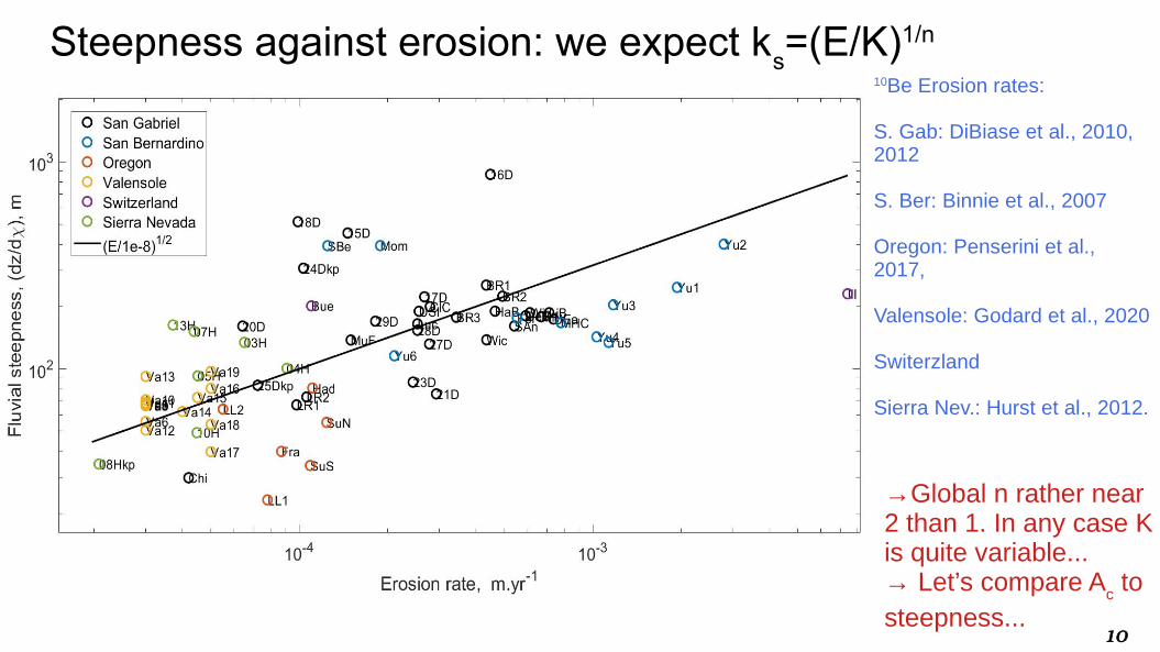
Steepness against erosion: we expect ks=(E/K)1/n

10Be Erosion rates:

S. Gab: DiBiase et al., 2010, 2012

S. Ber: Binnie et al., 2007

Oregon: Penserini et al., 2017,

Valensole: Godard et al., 2020

Switerzland

Sierra Nev.: Hurst et al., 2012.

→Global n rather near 2 than 1. In any case K is quite variable... → Let’s compare A

c to

steepness...

11

Debris-flow steepness match fluvial steepness

So knowing ks and S

df we can find A

c ! But what controls S

df ?

12

Debris-flow mechanics from granular model (courtesy S. McCoy/ L. McGuire)

(e.g. Sklar and Dietrich, 2004)Debris flow Erosion rate

Impact intensity

McCoy et al. (2012) McCoy et al. (2012)

Impact frequency

Volume eroded by impact

13

Implications of granular model scaling:

Edf∝H df( dzdx )ndf

, with ndf

~5-6, and Hdf the DF flow height, proportional to initial volume, V

i.

Further the long term erosion will depend on DF frequency, yielding: Edf∝F df V i( dzdx )ndf

At steady-state U=Edf and the F

dfV

i should be proportional to the sediment flux equal to UA

hs.

Assuming Ahs

= wcX

hs2 we obtain:

And therefore:

U=Edf∝U Xhs2 ( dzdx )

ndf

Sdf∝Xhs−2 /ndf

Can we validate this scaling ? What control Xhs

? If we assume a simple diffusive hillslope that ends when its gradient is reaching S

df, (i.e., S

df=UX

hs / D) we obtain :

Sdf∝(UD )2

(ndf+2) X hs∝(DU )ndf

(n df+2) → We also need to constrain D! For example by extracting hilltop curvature.

14

Estimation of Hilltop curvature and diffusivity

We implement a method similar to the one proposed by Hurst et al., 2012.

However CHT seems to increase sublinearly with E.

And thus D to increase with E.

15

Hillslope length and maximum slope:Diffusion theory : S

hs = U/D X ; U/D = C

HT. Is max(S

hs)=S

df ? → matches better E/0.01 than C

ht

Is the apparent increase in diffusion an artifact ?

Or U/D is different of C

HT , ?

because of soil depth variations ?

Anyway we next assume D=0.01 to try to predict X

hs, S

df

and Ac.

16

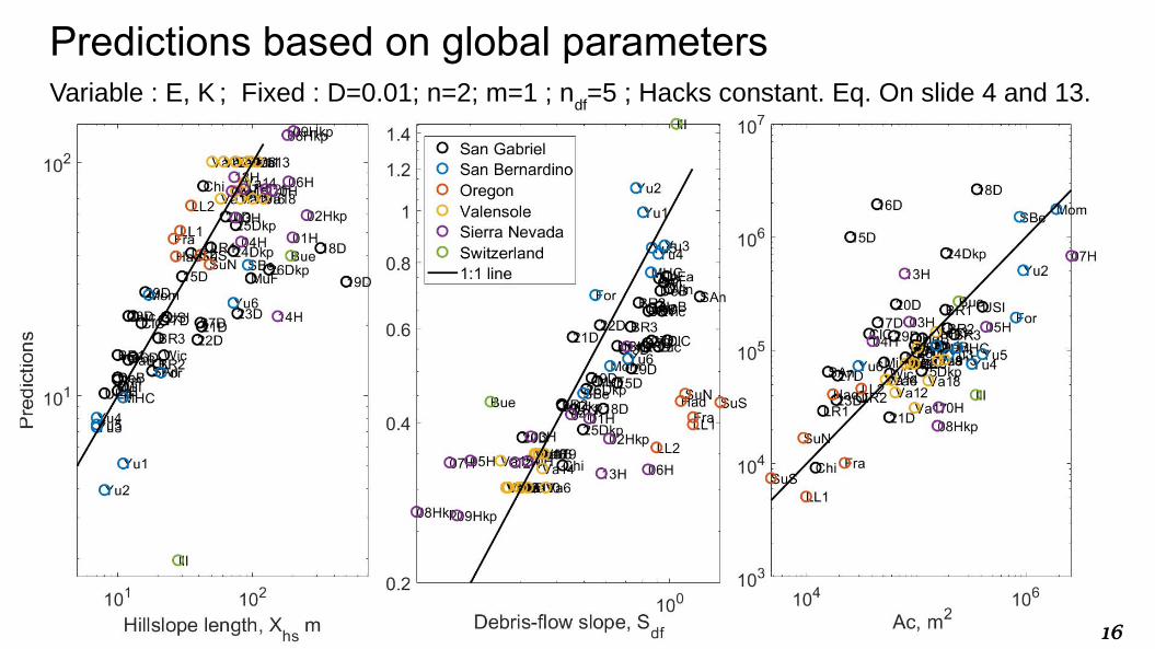
Predictions based on global parametersVariable : E, K

; Fixed : D=0.01; n=2; m=1 ; n

df=5 ; Hacks constant. Eq. On slide 4 and 13.

17

Conclusions:With LIDAR and 10Be data we constrained relations between erosion rate E, fluvial erodibility K, hillslope diffusivity D and debris flow parameters A

c and S

df. Our major findings are:

→ Fluvial network systematically overprinted by DF upstream of 0.5-5 km2. The upstream limit of SPIM can be found based on A

c, when knowing S

df and the steepness.

As a result a DF-corrected version of c is proposed and validated (as in Hergarten et al., 2016).

→ We found Sdf between 0.2 and 0.9, varying with E but also with the length of diffusive hillslopes, X

hs.

Although it does not match perfectly with our estimate of D based on curvature, the assumption that hillslopes are diffusive and end where their gradient reach S

df is fair.

→ The (bidirectional) coupling of Xhs and Sdf means that, knowing U, D and DF mechanics constant allow to predict X

hs and S

df. Then knowing fluvial steepness, A

c can be found and a profile from divide to

the fluvial domain can be fully predicted.

Future work : → Include variable m/n (in this presentation we fixed m/n=0.5, often but not always matching the best-fit to the data…)

→ Better understand the relations between E, D and Cht .

→ Implement the predictions into the numerical model DAC (Divide And Capture).

what controls the transition from fluvial regime to a

Documents