what constitutes a field experiment in economics?
TRANSCRIPT
What Constitutes a Field Experiment in Economics?
by
Glenn W. Harrison and John A. List †
June 2003
ABSTRACT
Experimental economists are leaving the reservation. They are recruiting subjects inthe field rather than in the classroom, using field goods rather than inducedvaluations, and using field context rather than abstract terminology in instructions.We argue that there is something methodologically fundamental behind this trend.Field experiments differ from laboratory experiments in many ways. Although it istempting to view field experiments as simply less controlled variants of laboratoryexperiments, we argue that to do so would be to seriously mischaracterize them.What passes for “control” in laboratory experiments might in fact be precisely theopposite if it is artificial to the subject or context of the task. We propose six factorsthat can be used to determine the field context of an experiment: the nature of thesubject pool, the nature of the information that the subjects bring to the task, thenature of the commodity, the nature of the task or trading rules applied, the natureof the stakes, and the environment that subjects operate in.
† Department of Economics, College of Business Administration, University of Central Florida, andDepartment of Agricultural and Resource Economics, University of Maryland, respectively. E-mail contacts: [email protected] and [email protected]. We are grateful toR. Mark Isaac and Charles Plott for comments.

Table of Contents
1. Defining Field Experiments . . . . . . . . . . . . . . . . . . . . . . . . . . . . . . . . . . . . . . . . . . . . . . . . . . . . . . -3-A. Criteria that Define Field Experiments . . . . . . . . . . . . . . . . . . . . . . . . . . . . . . . . . . . . . . -4-B. A Proposed Taxonomy . . . . . . . . . . . . . . . . . . . . . . . . . . . . . . . . . . . . . . . . . . . . . . . . . . -7-
2. The Nature of the Subject Pool . . . . . . . . . . . . . . . . . . . . . . . . . . . . . . . . . . . . . . . . . . . . . . . . . . . -8-A. Sample Selection in the Field . . . . . . . . . . . . . . . . . . . . . . . . . . . . . . . . . . . . . . . . . . . . . . -9-B. Are Students Different? . . . . . . . . . . . . . . . . . . . . . . . . . . . . . . . . . . . . . . . . . . . . . . . . . . -11-C. Precursors . . . . . . . . . . . . . . . . . . . . . . . . . . . . . . . . . . . . . . . . . . . . . . . . . . . . . . . . . . . . -16-
3. The Nature of the Information Subjects Already Have . . . . . . . . . . . . . . . . . . . . . . . . . . . . . . . -19-
4. The Nature of the Commodity . . . . . . . . . . . . . . . . . . . . . . . . . . . . . . . . . . . . . . . . . . . . . . . . . . . -20-A. Abstraction Requires Abstracting . . . . . . . . . . . . . . . . . . . . . . . . . . . . . . . . . . . . . . . . . -21-B. Field Goods Have Field Substitutes . . . . . . . . . . . . . . . . . . . . . . . . . . . . . . . . . . . . . . . -23-
The Natural Context of Substitutes . . . . . . . . . . . . . . . . . . . . . . . . . . . . . . . . . . . . -23-The Artificial Context of Substitutes . . . . . . . . . . . . . . . . . . . . . . . . . . . . . . . . . . . -23-
5. The Nature of the Task . . . . . . . . . . . . . . . . . . . . . . . . . . . . . . . . . . . . . . . . . . . . . . . . . . . . . . . . . -26-A. Who Cares If Hamburger Flippers Violate EUT? . . . . . . . . . . . . . . . . . . . . . . . . . . . . . -26-B. “Context” Is Not a Dirty Word . . . . . . . . . . . . . . . . . . . . . . . . . . . . . . . . . . . . . . . . . . . -30-
6. The Nature of the Stakes . . . . . . . . . . . . . . . . . . . . . . . . . . . . . . . . . . . . . . . . . . . . . . . . . . . . . . . -31-A. Taking the Stakes to Subjects Who Are Relatively Poor . . . . . . . . . . . . . . . . . . . . . . . -32-B. Taking the Task to the Subjects Who Care About It . . . . . . . . . . . . . . . . . . . . . . . . . . -34-
7. The Nature of the Environment . . . . . . . . . . . . . . . . . . . . . . . . . . . . . . . . . . . . . . . . . . . . . . . . . -37-A. Experimental Site . . . . . . . . . . . . . . . . . . . . . . . . . . . . . . . . . . . . . . . . . . . . . . . . . . . . . . -38-B. Experimental Proclamation . . . . . . . . . . . . . . . . . . . . . . . . . . . . . . . . . . . . . . . . . . . . . . . -39-C. Three Examples of Minimally Invasive Experiments . . . . . . . . . . . . . . . . . . . . . . . . . . -40-
Committees in the Field . . . . . . . . . . . . . . . . . . . . . . . . . . . . . . . . . . . . . . . . . . . . . -40-Betting in the Field . . . . . . . . . . . . . . . . . . . . . . . . . . . . . . . . . . . . . . . . . . . . . . . . . -41-Begging in the Field . . . . . . . . . . . . . . . . . . . . . . . . . . . . . . . . . . . . . . . . . . . . . . . . . -42-
8. “Natural Experiments,” An Oxymoron . . . . . . . . . . . . . . . . . . . . . . . . . . . . . . . . . . . . . . . . . . . -44-A. General Issues . . . . . . . . . . . . . . . . . . . . . . . . . . . . . . . . . . . . . . . . . . . . . . . . . . . . . . . . . -44-B. Inferring Discount Rates by Heroic Extrapolation . . . . . . . . . . . . . . . . . . . . . . . . . . . . -44-
Replication and Recalculation . . . . . . . . . . . . . . . . . . . . . . . . . . . . . . . . . . . . . . . . . -46-An Extension to Consider Uncertainty . . . . . . . . . . . . . . . . . . . . . . . . . . . . . . . . . -51-
9. Social Experiments . . . . . . . . . . . . . . . . . . . . . . . . . . . . . . . . . . . . . . . . . . . . . . . . . . . . . . . . . . . . -55-A. What Constitutes a Social Experiment in Economics? . . . . . . . . . . . . . . . . . . . . . . . . . -55-B. Methodological Lessons . . . . . . . . . . . . . . . . . . . . . . . . . . . . . . . . . . . . . . . . . . . . . . . . . -57-
Recruitment and the Evaluation Problem . . . . . . . . . . . . . . . . . . . . . . . . . . . . . . . -57-Substitution and the Evaluation Problem . . . . . . . . . . . . . . . . . . . . . . . . . . . . . . . -59-Experimenter Effects . . . . . . . . . . . . . . . . . . . . . . . . . . . . . . . . . . . . . . . . . . . . . . . -59-
10. Conclusion . . . . . . . . . . . . . . . . . . . . . . . . . . . . . . . . . . . . . . . . . . . . . . . . . . . . . . . . . . . . . . . . . . -62-
References . . . . . . . . . . . . . . . . . . . . . . . . . . . . . . . . . . . . . . . . . . . . . . . . . . . . . . . . . . . . . . . . . . . . . -63-

1 Imagine a classroom setting in which the class breaks up into smaller tutorial groups. In some groups a videocovering certain material is presented, in another group a free discussion is allowed, and in another group there is a moretraditional lecture. Then the grades of the students in each group are examined after they have taken a common exam.Assuming that all of the other features of the experiment are controlled, such as which student gets assigned to whichgroup, this experiment would not seem unnatural to the subjects. They are all students doing what comes naturally tostudents, and these three teaching alternatives are each standardly employed. Along similar lines in economics, albeitwith simpler technology and less control than one might like, see Duddy [1924].
-1-
Experimental economists are leaving the reservation. They are recruiting subjects in the field
rather than in the classroom, using field goods rather than induced valuations, and using field
context rather than abstract terminology in instructions. We argue that there is something
methodologically fundamental behind this trend. Field experiments differ from laboratory
experiments in many ways. Although it is tempting to view field experiments as simply less
controlled variants of laboratory experiments, we argue that to do so would be to seriously
mischaracterize them. What passes for “control” in laboratory experiments might in fact be precisely
the opposite if it is artificial to the subject or context of the task. In the end, we see field experiments
as being methodologically complementary to traditional laboratory experiments.
Our primary point is that the notion of a field experiment defines what might be better
called an ideal experiment, in the sense that one is able to observe a subject in a controlled setting
but where the subject does not perceive any of the controls as being unnatural and there is no
deception being practiced. At first blush the idea that one can observe subjects in a natural setting
and yet have controls might seem contradictory, but we will argue that it is not.1
Our second point is that many of the characteristics of field experiments can be found in
varying degrees in lab experiments. Thus, many of the characteristics that people identify with field
experiments are not only found in field experiments, and should not be used to differentiate them
from lab experiments.
Our third point, related to the first two, is that there is much to learn from field experiments
-2-
when one goes back into the lab. The unexpected things that happen when one loosens control in
the field are often indicators of key features of the economic transaction that have been neglected in
the lab. Thus field experiments can help one design better lab experiments, and have a
methodological role quite apart from their complementarity at a substantive level.
In section 1 we offer a typology of field experiments in the literature, identifying the key
characteristics defining the species. We suggest some terminology to better identify different types of
field experiments, or more accurately to identify different characteristics of field experiments. We do
not propose a bright line to define some experiments as field experiments and others as something
else, but a set of criteria that one would expect to see in varying degrees in a field experiment. We
propose six factors that can be used to determine the field context of an experiment: the nature of
the subject pool, the nature of the information that the subjects bring to the task, the nature of the
commodity, the nature of the task or trading rules applied, the nature of the stakes, and the
environment the subjects operate in. In sections 2 through 7 we examine each of these factors in
turn.
In sections 8 and 9 we review two types of experiments that may be contrasted with ideal
field experiments. One might be called a “natural experiment,” even though that expression is an
oxymoron in the same sense that “self-insurance” is. The idea is to recognize that some event that
naturally occurs in the field happens to have some of the characteristics of a field experiment. These
can be attractive sources of data on large-scale economic transactions, but usually at some cost due
to the lack of control.
The other type of experiment is a social experiment, in the sense that it is a deliberate part of
social policy by the government. Social experiments involve deliberate, randomized changes in the
manner in which some government program is implemented. They have become popular in certain

-3-
areas, such as employment schemes and the detection of discrimination. Their disadvantages have
been well documented, given their political popularity, and there are several important
methodological lessons from those debates for the design of field experiments.
1. Defining Field Experiments
There are several ways to define words. One is to ascertain the formal definition by looking
it up in the dictionary. Another is to identify what it is that you want the word-label to differentiate.
The Oxford English Dictionary (Second Edition) defines the word “field” in the following
manner: “Used attributively to denote an investigation, study, etc., carried out in the natural
environment of a given material, language, animal, etc., and not in the laboratory, study, or office.”
This orients us to think of the natural environment of the different components of an experiment.
It is important to identify what factors make up a field experiment so that we can
functionally identify what factors drive results in different experiments. To give a direct example of
the type of problem that motivated us, when List [2001] gets results in a field experiment that differ
from the counterpart lab experiments of Cummings, Harrison and Osborne [1995] and Cummings
and Taylor [1999], what explains the difference? Is it the use of data from a particular market whose
participants have selected into the market instead of student subjects, the use of subjects with
experience in related tasks, the use of private sports-cards as the underlying commodity instead of an
environmental public good, the use of streamlined instructions, the less-intrusive experimental
methods, or is it some combination of these and similar differences? We believe field experiments
have matured to the point that some framework for addressing such differences in a systematic
manner is necessary.
-4-
A. Criteria that Define Field Experiments
We propose six factors that can be used to determine the field context of an experiment:
! the nature of the subject pool,
! the nature of the information that the subjects bring to the task,
! the nature of the commodity,
! the nature of the task or trading rules applied,
! the nature of the stakes, and
! the nature of the environment that the subject operates in.
The taxonomy that results will be important, we believe, as comparisons between lab and field
experimental results become more common.
Student subjects can be viewed as the standard subject pool used by experimenters, simply
because they are a convenience sample for academics. Thus when one goes “outdoors” and uses
field subjects, they should be viewed as non-standard in this sense. But we argue that the use of non-
standard subjects should not automatically qualify the experiment as a field experiment. The
experiments of Cummings, Harrison and Rutström [1995], for example, used individuals recruited
from churches in order to obtain a wider range of demographic characteristics than one would
obtain in the standard college setting. The importance of a non-standard subject pool varies from
experiment to experiment: in this case it simply provided a less concentrated set of socio-
demographic characteristics with respect to age and education level, which turned out to be
important when developing statistical models to adjust for hypothetical bias (Blackburn, Harrison
and Rutström [1994]). Alternatively, the subject pool can be designed to represent the national
population, so that one can make better inferences about the general population (Harrison, Lau and
Williams [2002]).

2 It is worth noting that Smith [1962] did not use real payoffs to motivate subjects in his experiments, althoughhe does explain how that could be done and reports one experiment (fn 9., p.121) in which monetary payoffs wereemployed.
-5-
In addition, non-standard subject pools might bring experience with the commodity or the
task to the experiment, quite apart from their wider array of demographic characteristics. In the
field, subjects bring certain information to their trading activities in addition to their knowledge of
the trading institution. In abstract settings the importance of this information is diminished, by
design, and that can lead to changes in the way that individuals behave. For example, absent such
information, risk aversion can lead to subjects requiring a risk premium when bidding for objects
with uncertain characteristics.
The commodity itself can be an important part of the field. Recent years have seen a growth
of experiments concerned with eliciting valuations over actual goods, rather than using induced
valuations over virtual goods. The distinction here is between physical goods or actual services and
abstractly defined goods. The latter have been the staple of experimental economics since Smith
[1962], but imposes an artificiality that could be a factor influencing behavior.2 Such influences are
actually of great interest, or should be. If the nature of the commodity itself affects behavior, in a
way that is not accounted for by the theory being applied, then the theory has at best a limited
domain of applicability that we should know about, and at worse is simply false. In either case, one
can know the limitations of the generality of theory only if one tests for it, by considering physical
goods and services.
Again, however, just having one field characteristic, in this case a physical good, does not
constitute a field experiment in any fundamental sense. Rutström [1998] sold lots and lots of
chocolate truffles in a laboratory study of different auction institutions designed to elicit values
truthfully, but hers was very much a lab experiment despite the tastiness of the commodity.

3 We would exclude experiments in which the commodity was a gamble, since very few of those gambles takethe form of naturally occurring lotteries.
-6-
Similarly, Bateman et al. [1997] elicited valuations over pizza and dessert vouchers for a local
restaurant. While these commodities were not actual pizza or dessert themselves, but vouchers
entitling the subject to obtain them, they are not abstract. There are many other examples in the
experimental literature of designs involving physical commodities.3
The nature of the task that the subject is being asked to undertake is an important
component of a field experiment, since one would expect that field experience could play a major
role in helping individuals develop heuristics for specific tasks. The lab experiments of Kagel and
Levin [1999] illustrate this point, with “super-experienced” subjects behaving differently than
inexperienced subjects in terms of their propensity to fall prey to the winners’ curse. An important
question is whether the successful heuristics that evolve in certain field settings “travel” to other field
and lab settings (Harrison and List [2003]). Another aspect of the task is the specific
parameterization that is adopted in the experiment. One can conduct a lab experiment with
parameter values estimated from field data, so as to study lab behavior in a “field-relevant” domain.
Since theory is often domain-specific, and behavior can always be, this is an important component
of the interplay between lab and field. Early illustrations of the value of this approach include
Grether, Isaac and Plott [1981][1989], Grether and Plott [1984] and Hong and Plott [1982].
The nature of the stakes can also affect field responses. Stakes in the laboratory might be
very different than those encountered in the field, and hence have an effect on behavior. If
valuations are taken seriously when they are in the tens of dollars, or in the hundreds, but are made
indifferently when the price when it is less than $1, laboratory experiments with stakes below $1
could easily engender imprecise bids. Of course, people buy inexpensive goods in the field as well,

4 The fact that the rules are imposed does not imply that the subjects would reject them, individually or socially,if allowed to.
5 To offer an early and a recent example, consider the risk aversion experiments conducted by Binswanger[1980][1981] in India, and Harrison, Lau and Williams [2002], who took the lab experimental design of Coller andWilliams [1999] into the field with a representative sample of the Danish population.
-7-
but the valuation process they use might be keyed to different stake levels. Alternatively, field
experiments in relatively poor countries offer the opportunity to evaluate the effects of substantial
stakes within a given budget.
The environment of the experiment can also influence behavior. The environment can
provide context to suggest strategies and heuristics that a lab setting might not. Lab experimenters
have always worried that the use of classrooms might engender role-playing behavior, and indeed
this is one of the reasons that experimental economists are generally suspicious of experiments
without salient monetary rewards. Even with salient rewards, however, environmental effects could
remain. Rather than view them a uncontrolled effects, we see them as worthy of controlled study.
B. A Proposed Taxonomy
Any taxonomy of field experiments runs the risk of missing important combinations of the
factors that differentiate field experiments from conventional lab experiments. However, there is
some value in having broad terms to differentiate what we see as the key differences. We propose
the following terminology:
! a conventional lab experiment is one that employs a standard subject pool of students, an abstract
framing, and an imposed4 set of rules;
! a synthetic field experiment is the same as a conventional lab experiment but with a non-standard
subject pool;5
! a framed field experiment is the same as a synthetic field experiment but with field context in

6 For example, the experiments of Bohm [1984b] to elicit valuations for public goods that occurred naturally inthe environment of subjects, albeit with unconventional valuation methods; or the Vickrey auctions and “cheap talk”scripts that List [2001] conducted with sport card collectors, using sports cards as the commodity and at a show wherethey trade such commodities.
7 For example, the manipulation of betting markets by Camerer [1998], or the solicitation of charitablecontributions by List and Lucking-Reiley [2002].
8 For example, Harrison and List [2003] conduct synthetic field experiments and framed field experiments withthe same subject pool, precisely to identify how well the heuristics that might apply naturally in the latter setting “travel”to less context-ridden environments found in the former setting.
-8-
either the commodity, task, or information set that the subjects can use;6
! a natural field experiment is the same as a framed field experiment but where the environment is
one where the subjects naturally undertake these tasks and where the subjects do not know
that they are in an experiment.7
We recognize that any such taxonomy leaves some gaps. Moreover, it is often appropriate to
conduct several types of experiments in order to identify the issue of interest.8
2. The Nature of the Subject Pool
A common criticism of the relevance of inferences drawn from laboratory experiments is
that one needs to undertake an experiment with “real” people, not students. This criticism is often
deflected by experimenters with the following imperative: if you think that the experiment will
generate different results with “real” people, then go ahead and run the experiment with real people.
A variant of this response is to challenge the critics’ assertion that students are not representative. As
we will see, this variant is more subtle and constructive than the first response.
The first response, to suggest that the critic go and run the experiment with real people, is
often adequate to get rid of unwanted referees at academic journals. In practice, however, few
experimenters ever go out in the field in a serious and large-sample way. It is relatively easy to say
that the experiment could be applied to real people, but to actually do so entails some serious and

-9-
often unattractive logistical problems.
A more substantial response to this criticism is to consider what it is about students that is
viewed, a priori, as being non-representative of the target population. There are at least two issues
here. The first is whether endogenous sample selection or attrition has occurred due to incomplete
control over recruitment and retention, so that the observed sample is unreliable in some statistical
sense (e.g., generating inconsistent estimates of treatment effects). The second is whether the
observed sample can be informative on the behavior of the population, assuming away sample
selection issues.
A. Sample Selection in the Field
Conventional lab experiments typically use students who are recruited after being told only
general statements about the experiment. By and large, recruitment procedures avoid mentioning
the nature of the task, or the expected earnings. Most lab experiments are also one-shot, in the
sense that they do not involve repeated observations of a sample subject to attrition. Of course,
neither of these features is essential. If one wanted to recruit subjects with specific interest in a task,
it would be easy to do (e.g., Bohm and Lind [1993]). And if one wanted to recruit subjects for
several sessions, to generate “super-experienced” subjects or to conduct pre-tests of such things as
risk aversion, that could be built into the design as well (e.g., Kagel and Levin [1986][1999][2002] or
Harrison, Johnson, McInnes, and Rutström [2003]).
One concern with lab experiments conducted with convenience samples of students is that
students might be self-selected in some way, so that they are a sample that excludes certain
individuals with characteristics that are important determinants of underlying population behavior.
Although this problem is a severe one, its potential importance in practice should not be
-10-
overemphasized. It is always possible to simply inspect the sample to see if certain strata of the
population are not represented, at least under the tentative assumption that it is only observables
that matter. In this case it would behoove the researcher to augment the initial convenience sample
with a quota sample, in which the missing strata were surveyed. Thus one tends not to see many
convicted mass murderers or brain surgeons in student samples, but we certainly know where to go
if we feel the need to include them in our sample.
Another consideration, of increasing importance for experimenters, is the possibility of
recruitment biases in our procedures. One aspect of this issue is studied by Rutström [1998]. She
examines the role of recruitment fees in biasing the samples of subjects that are obtained. The
context for her experiment is particularly relevant here since it entails the elicitation of values for a
private commodity. She finds that there are some significant biases in the strata of the population
recruited as one varies the recruitment fee from zero dollars to two dollars, and then up to ten
dollars. However, an important finding is that most of those biases can be corrected simply by
incorporating the relevant characteristics in a statistical model of the behavior of subjects and
thereby controlling for them. In other words, it does not matter if one group of subjects in one
treatment has 60% females and the other sample of subjects in another treatment has only 40%
females, providing one controls for the difference in gender when pooling the data and examining
the key treatment. This is a situation in which gender might influence the response or the effect of
the treatment, but controlling for gender allows one to remove this recruitment bias from the
resulting inference.
However, field experiments face a more serious problem of sample selection that depends
on the nature of the task. Once the experiment has begun it is not as easy as it is in the lab to
control information flow about the nature of the task. This is obviously a matter of degree, but can

9 If not to treatment, then randomization often occurs over choices to determine payoff.10 The contingent valuation method refers to the use of hypothetical field surveys to value the environment, by
posing a scenario that asks the subject to place a value on an environmental change contingent on a market for itexisting. See Cummings and Harrison [1994] for a critical review of the role of experimental economics in this field.
-11-
lead to endogenous subject attrition from the experiment. Such attrition is actually informative
about subject preferences, since the subject’s exit from the experiment indicates that the subject had
made a negative evaluation of it (Philipson and Hedges [1998]).
The classic problem of sample selection refers to possible recruitment biases, such that the
observed sample is generated by a process that depends on the nature of the experiment. This
problem can be serious for any experiment, since a hallmark of virtually every experiment is the use
of some randomization, typically to treatment.9 If the population from which volunteers are being
recruited has divers risk attitudes, and plausibly expects the experiment to have some element of
randomization, then the observed sample will tend to look less risk averse than the population. It is
easy to imagine how this could then affect behavior differentially in some treatments. Heckman and
Smith [1995] discuss this issue in the context of social experiments, but the concern applies equally
to field and lab experiments.
B. Are Students Different?
This question is addressed by Harrison and Lesley [1996] (HL). They approach this question
in a simple statistical framework. Indeed they do not consider the issue in terms of the relevance of
experimental methods, but rather in terms of the relevance of convenience samples for the
contingent valuation method.10 However, it is easy to see that their methods apply much more
generally.
The HL approach may be explained in terms of their attempt to mimic the results of a large-

11 The exact form of that statistical model is not important for illustrative purposes, although the developmentof an adequate statistical model is important to the reliability of this method.
-12-
scale national survey conducted for the Exxon Valdez oil spill litigation. A major national survey was
undertaken in this case by Carson et al. [1992][1994] for the Attorney General of the State of Alaska.
This survey used then-state-of-the-art survey methods but, more importantly for present purposes,
used a full probability sample of the nation. HL ask if one can obtain essentially the same results
using a convenience sample of students from the University of South Carolina. Using students as a
convenience sample is largely a matter of methodological bravado. One could readily obtain
convenience samples in other ways, but using students provides a tough test of their approach.
They proceeded by developing a simpler survey instrument than the one used in the original
study. The purpose of this is purely to facilitate completion of the survey and is not essential to the
use of the method. This survey was then administered to a relatively large sample of students. An
important part of the survey, as in any field survey that aims to control for subject attributes, is the
collection of a range of standard socio-economic characteristics of the individual (e.g., sex, age,
income, parental income, number of people in the household, and marital status). Once these data
are collated a statistical model is developed in order to explain the key responses in the survey. In
this case the key response is a simple “yes” or “no” to a single dichotomous choice valuation
question. In other words, the subject was asked whether he or she would be willing to pay $X
towards a public good, where $X was randomly selected to be $10, $30, $60 or $120. A subject
would respond to this question with a “yes”, a “no”, or a “not sure.” A simple statistical model is
developed to explain behavior as a function of the observable socio-economic characteristics.11
Assuming that a statistical model has been developed, HL then proceed to the key stage of
their method. This is to assume that the coefficient estimates from the statistical model based on the
12 For example, assume a population of 50% men and 50% women, but where a sample drawn at randomhappens to have 60% men. If responses differ according to sex, predicting the population is simply a matter of re-weighting the survey responses. We offer a counter-example in section 8.
-13-
student sample apply to the population at large. If this is the case, or if this assumption is simply
maintained, then the statistical model may be used to predict the behavior of the target population if
one can obtain information about the socioeconomic characteristics of the target population.
The essential idea of the HL method is simple and more generally applicable than this
example suggests. If students are representative in the sense of allowing the researcher to develop a
“good” statistical model of the behavior under study, then one can often use publicly available
information on the characteristics of the target population to predict the behavior of that
population. Their fundamental point is that the “problem with students” is the lack of variability in
their socio-demographic characteristics, not necessarily the unrepresentativeness of their behavioral
responses conditional on their socio-demographic characteristics.
To the extent that student samples exhibit limited variability in some key characteristics, such
as age, then one might be wary of the veracity of the maintained assumption involved here.
However, the sample does not have to look like the population in order for the statistical model to be
an adequate one for predicting the population response.12 All that is needed is for the behavioral
responses of students to be the same as the behavioral responses of non-students. This can either
be assumed a priori or, better yet, tested by sampling non-students as well as students.
Of course, it is always better to be forecasting on the basis of an interpolation rather than an
extrapolation, and that is the most important problem one has with student samples. This issue is
discussed in some detail by Blackburn, Harrison, and Rutström [1994]. They estimated a statistical
model of subject response using a sample of college students and also estimated a statistical model
of subject response using field subjects drawn from a wide range of churches in the same urban area.

13 On the other hand, reporting large variances may be the most accurate reflection of the wide range ofvaluations held by this sample. We should not always assume that distributions with smaller variances provide moreaccurate reflections of the underlying population just because they have little dispersion; for this to be true many auxiliaryassumptions about randomness of the sampling process must be assumed, not to mention issues about the stationarity ofthe underlying population process. This stationarity is often assumed away in contingent valuation research (e.g., theproposal to use double-bounded dichotomous choice formats without allowing for possible correlation between the twoquestions).
-14-
Each were convenience samples. The only difference is that the church sample exhibited a much
wider variability in their socio-demographic characteristics. In the church sample ages ranged from
21 to 79; in the student sample ages ranged from 19 to 27. When predicting behavior of students
based on the church-estimated behavioral model, interpolation was used and the predictions were
extremely accurate. However, in the reverse direction, when predicting church behavior from the
student-estimated behavioral model, the predictions were disastrous in the sense of having extremely
wide forecast variances.13 The reason is simple to understand. It is much easier to predict the
behavior of a 26-year-old when one has a model that is based on the behavior of people whose ages
range from 21 up to 79 than it is to estimate the behavior of a 69-year-old based on the behavioral
model from a sample whose ages range from 19 to 27.
What is the relevance of these methods for the original criticism of experimental procedures?
Think of the experimental subjects as the convenience sample in the HL approach. The lessons that
are learned from this student sample could be embodied in a statistical model of their behavior and
implications drawn for a larger target population. Although this approach rests on an assumption
that is as yet untested, concerning the representativeness of student behavioral responses conditional
on their characteristics, it does provide a simple basis for evaluating the extent to which conclusions
about students apply to a broader population.
How could this method ever lead to interesting results? The answer depends on the context.
Consider a situation in which the behavioral model showed that age was an important determinant

-15-
of behavior. Consider further a situation in which the sample used to estimate the model had an
average age that was not representative of the population as a whole. In this case it is perfectly
possible that the responses of the student sample could be quite different than the predicted
responses of the population. Although no such instances have appeared in the applications of this
method thus far, they should not be ruled out.
We conclude, therefore, that many of the concerns raised by this criticism, while valid, are
able to be addressed by simple extensions of the methods that experimenters currently use.
Moreover, these extensions would increase the general relevance of experimental methods obtained
with student convenience samples.
Further problems arise if one allows unobserved individual effects to play a role. In some
statistical settings it is possible to allow for those effects by means of “fixed effect” or “random
effects” analyses. But these standard devices, now quite common in the tool-kit of experimental
economists, do not address a deeper problem. The internal validity of a randomized design is
maximized when one knows that the samples in each treatment are identical. This happy extreme
leads many to infer that matching subjects on a finite set of characteristics must be better in terms of
internal validity than not matching them on any characteristics.
But partial matching can be worse than no matching. The most important example of this is
due to Heckman and Siegelman [1993] and Heckman [1998], who critique paired-audit tests of
discrimination. In these experiments two applicants for a job are matched in terms of certain
observables, such as age, sex, and education, and differ in only one protected characteristic, such as
race. However, unless some extremely strong assumptions about how characteristics map into
wages are made, there will be a pre-determined bias in outcomes. The direction of the bias
“depends,” and one cannot say much more. A metaphor from Heckman [1998; p.110] illustrates.

-16-
Boys and girls of the same age are in a high jump competition, and jump the same height on average.
But boys have a higher variance in their jumping technique, for any number of reasons. If the bar is
set very low relative to the mean, then the girls will look like better jumpers; if the bar is set very
high then the boys will look like better jumpers. The implications for numerous (lab and field)
experimental studies of the effect of gender, that do not control for other characteristics, should be
apparent.
C. Precursors
Several experimenters have deliberately sought out subjects in the “wild,” or brought
subjects from the “wild” in to labs. It is notable that this effort has occurred from the earliest days
of experimental economics, and that it has only recently become common.
Lichtenstein and Slovic [1973] replicated their earlier experiments on “preference reversals”
in “... a nonlaboratory real-play setting unique to the experimental literature on decision processes –
a casino in downtown Las Vegas” (p. 17). The experimenter was a professional dealer, and the
subjects were drawn from the floor of the casino. Although the experimental equipment may have
been relatively forbidding (it included a PDP-7 computer, a DEC-339 CRT, and a keyboard), the
goal was to identify gamblers in their natural habitat. The subject pool of 44 did include 7 known
dealers that worked in Las Vegas, and the “... dealer’s impression was that the game attracted a
higher proportion of professional and educated persona than the usual casino clientele” (p. 18).
Kagel, Battalio and Walker [1979] provide a remarkable, early examination of many of the
issues we raise. They were concerned with “volunteer artifacts” in lab experiments, ranging from

14 They also have a discussion of the role that these possible biases play in social psychology experiments, andhow they have been addressed there.
15 And either inexperienced, once experienced, or twice experienced in asset market trading.
-17-
the characteristics that volunteers have to the issue of sample selection bias.14 They conducted a
field experiment in the homes of the volunteer subjects, examining electricity demand in response to
changes in prices, weekly feedback on usage, and energy conservation information. They also
examined a comparison sample drawn from the same population, to check for any biases in the
volunteer sample.
Binswanger [1980][1981] conducted experiments eliciting measures of risk aversion from
farmers in rural India. Apart from the policy interest of studying agents in developing countries, one
stated goal of using field experiments was to assess risk attitudes for choices in which the income
from the experimental task was a substantial fraction of the wealth or annual income of the subject.
The method he developed has been used recently in conventional laboratory settings with student
subjects by Holt and Laury [2002].
Burns [1985] conducted induced value market experiments with floor traders from wool
markets, to compare with the behavior of student subjects in such settings. The goal was to see if the
heuristics and decision rules these traders evolved in their natural field setting affected their
behavior. She did find that their natural field rivalry had a powerful motivating effect on their
behavior.
Smith, Suchanek and Williams [1988] conducted a large series of experiments with student
subjects in an “asset bubble” experiment. In the 22 experiments they report, 9 to 12 traders with
experience in the double-auction institution15 traded a number of 15 or 30 period assets with the
same common value distribution of dividends. If all subjects are risk neutral, and have common
16 There are only two reasons why players may want to trade in this market. First, if players differ in their riskattitudes then we might see the asset trading below expected dividend value (since more risk averse players will pay lessrisk averse players a premium over expected dividend value to take their assets). Second, if subjects have diverse priceexpectations we can expect trade to occur because of expected capital gains. This second reason for trading (diverse priceexpectations) can actually lead to contract prices above expected dividend value as long as some subject believes thatthere are other subjects who believe the price will go even higher.
17 Harrison [1992b] reviews the detailed experimental evidence on bubbles, and shows that very few significantbubbles occur with subjects that are experienced in asset market experiments in which there is a short-lived asset, such asthose under study. A bubble is significant only if there is some non-trivial volume associated with it.
-18-
price expectations, then there would be no reason for trade in this environment.16 The major
empirical result is the large number of observed price bubbles: 14 of the 22 experiments can be said
to have had some price bubble.
In an effort to address the criticism that bubbles were just a manifestation of using student
subjects, Smith, Suchanek and Williams [1988] recruited non-student subjects for one experiment.
As they put it, one experiment “... is noteworthy because of its use of professional and business
people from the Tucson community, as subjects. This market belies any notion that our results are
an artifact of student subjects, and that businessmen who ‘run the real world’ would quickly learn to
have rational expectations. This is the only experiment we conducted that closed on a mean price
higher than in all previous trading periods” (p. 1130-1). The reference at the end is to the
observation that the price bubble did not burst as the finite horizon of the experiment was
approaching. Another notable feature of this price bubble is that it was accompanied by heavy
volume, unlike the price bubbles observed with experienced subjects.17 Although these subjects were
not students, they were inexperienced in the use of the double auction experiments. Moreover, there
is no presumption that their field experience was relevant for this type of asset market.

-19-
3. The Nature of the Information Subjects Already Have
Auction theory provides a rich set of predictions concerning bidders’ behavior. One
particularly salient finding in a plethora of laboratory experiments that is not predicted in first price
common value auction theory is that bidders commonly fall prey to the winner’s curse. Only “super-
experienced” subjects, who are in fact recruited on the basis of not having lost money in previous
experiments, avoid it regularly. This would seem to suggest that experience is a sufficient condition
for an individual bidder to avoid the winner’s curse. Harrison and List [2003] show that this
implication is supported when one considers a natural setting in which it is relatively easy to identify
traders that are more or less experienced at the task. In their experiments the experience of subjects
is either tied to the commodity, the valuation task, and the use of auctions (in the field experiments
with sportscards), or simply to the use of auctions (in the laboratory experiments with induced
values). In all tasks, experience is generated in the field and not the lab. These results provide
support for the notion that context-specific experience does appear to carry over to comparable
settings, at least with respect to these types of auctions.
This experimental design emphasizes the identification of a naturally occurring setting in
which one can control for experience in the way that it is accumulated in the field. Experienced
traders gain experience over time by observing and surviving a relatively wide range of trading
circumstances. In some settings this might be proxied by the manner in which experienced or super-
experienced subjects are defined in the lab, but we doubt if the standard lab settings will reliably
capture the full extent of the field counterpart of experience. This is not a criticism of lab
experiments, just their domain of applicability.
The methodological lesson we draw is that one should be careful not to generalize from the
evidence of a winner’s curse by student subjects that have no experience at all with the field context.

18 See Harrison, Harstad and Rutström [2003] for a general treatment.
-20-
These results do not imply that every field context has experienced subjects, such as professional
sportscard dealers, that avoid the winner’s curse. Instead, they point to a more fundamental need to
consider the field context of experiments before drawing general conclusions. It is not the case that
abstract, context-free experiments provide more general findings if the context itself is relevant to the performance of
subjects. In fact, one would generally expect such context-free experiments to be unusually tough
tests of economic theory, since there is no control for the context that subjects might themselves impose on the
abstract experimental task.
The main result is that if one wants to draw conclusions about the validity of theory in the
field, then one must pay attention to the myriad ways in which field context can affect behavior. We
believe that conventional lab experiments, in which roles are exogenously assigned and defined in an
abstract manner, cannot ubiquitously provide reliable insights into field behavior. One might be able
to modify the lab experimental design to mimic those field contexts more reliably, and that would
make for a more robust application of the experimental method in general.
4. The Nature of the Commodity
Many field experiments involve real, physical commodities and the values that subjects place
on them in their daily life. This is distinct from the traditional focus in experimental economics on
experimenter-induced valuations on an abstract commodity, often referred to as “tickets” just to
emphasize the lack of any field referent that might suggest a valuation. The use of real commodities,
rather than abstract commodities, is not unique to the field, nor does one have to eschew
experimenter-induced valuations in the field. But the use of real goods does have consequences that
apply to both lab and field experiments.18

-21-
A. Abstraction Requires Abstracting
One simple example is the Tower of Hanoi game which has been extensively studied by
cognitive psychologists (e.g., Hayes and Simon [1974]) and more recently by economists (McDaniel
and Rutström [2001]) in some fascinating
experiments. The physical form of the game, as
found in all serious Montessori classrooms and
Pearl [1984; p.28], is shown below.
The top picture shows the initial state, in
which n disks are on peg 1. The goal is to move
all of the disks to peg 3, as shown in the goal state
in the bottom picture. The constraints are that
only one disk may be moved at a time, and no disk may ever lie under a bigger disk. The objective is
to reach the goal state in the least number of moves. The “trick” to solving the Tower of Hanoi is to
use backwards induction: visualize the final, goal state and use the constraints to figure out what the
penultimate state must have looked like (viz., the tiny disk on the top of peg 3 in the goal state
would have to be on peg 1 or peg 2 by itself). Then work back from that penultimate state, again
respecting the constraints (viz., the second smallest disk on peg 3 in the goal state would have to be
on whichever of peg 1 or peg 2 the smallest disk is not on). One more step in reverse and the
essential logic should be clear (viz., in order for the third largest disk on peg 3 to be off peg 3, one of
peg 1 or peg 2 will have to be cleared, so the smallest disk should be on top of the second smallest
disk).
Observation of students in Montessori classrooms makes it clear how they (eventually) solve
the puzzle, when confronted with the initial state. They shockingly violate the constraints and move
-22-
all the disks to the goal state en masse, and then physically work backwards along the lines of the
above thought experiment in backwards induction. The critical point here is that they temporarily
violate the constraints of the problem in order to solve it “properly.”
Contrast this behavior with the laboratory subjects in McDaniel and Rutström [2001]. They
were given a computerized version of the game, and told to try to solve it. However, the
computerized version did not allow them to violate the constraints. Hence the laboratory subjects
were unable to use the classroom Montessori method, by which the student learns the idea of
backwards induction by exploring it with physical referents. This is not a design flaw of the
McDaniel and Rutström [2001] lab experiments, but simply one factor to keep in mind when
evaluating the behavior of their subjects. Without the physical analogue of the final goal state being
allowed in the experiment, the subject was forced to visualize that state conceptually, and to likewise
imagine conceptually the penultimate states. Although that may encourage more fundamental
conceptual understanding of the idea of backwards induction, if attained, it is quite possible that it
posed an insurmountable cognitive burden for some of the experimental subjects.
It might be tempting to think of this as just two separate tasks, instead of a real commodity
and its abstract analogue. But we believe that this example does identify an important characteristic
of commodities in ideal field experiments: the fact that they allow subjects to adopt the
representation of the commodity and task that best suits their objective. In other words, the
representation of the commodity by the subject is an integral part of how the subject solves the task.
One simply cannot untangle them, at least not easily and naturally.
This example also illustrates that off-equilibrium states, in which one is not optimizing in
terms of the original constrained optimization task, may indeed be critical to the attainment of the

19 This is quite distinct from the valid point made by Smith [1982; p.934, fn.17], that it is appropriate to designthe experimental institution so as to make the task as simple and transparent as possible providing one holds constantthese design features as one compares experimental treatments. Such designs may make the results of less interest forthose wanting to make field inferences, but that is a tradeoff that every theorist and experimenter faces to varyingdegrees.
-23-
equilibrium state.19 Thus we should be mindful of possible field devices which allow subjects to
explore off-equilibrium states, even if those states are ruled out in our null hypothesis.
B. Field Goods Have Field Substitutes
There are two respects in which “field substitutes” play a role whenever one is conducting an
experiment with naturally occurring, or field, goods. We can refer to the former as the natural context
of substitutes, and to the latter as an artificial context of substitutes. The former needs to be captured
if reliable valuations are to be elicited; the latter needs to be minimized or controlled for.
The Natural Context of Substitutes
The first way in which substitutes play a role in an experiment is the traditional sense of
demand theory: to some individuals, a bottle of scotch may substitute for a Bible when seeking
Peace of Mind. The degree of substitutability here is the stuff of individual demand elasticities, and
can reasonably be expected to vary from subject to subject. The upshot of this consideration is, yet
again, that one should always collect information on observable individual characteristics and control
for them.
The Artificial Context of Substitutes
The second way in which substitutes play a role in an experiment is the more subtle issue of
affiliation which arises in lab or field settings that involve preferences over a field good. To see this

20 The theoretical and experimental literature makes this point clearly by comparing real-time English auctionswith sealed-bid Vickrey auctions: see Milgrom and Weber [1982] and Kagel, Harstad and Levin [1987]. The same logicthat applies for the one-shot English auction applies for a repeated Vickrey auction, even if the specific biddingopponents were randomly drawn from the population in each round.
21 The term “bidding behavior” is used to allow for information about bids as well as non-bids. In therepeated Vickrey auction it is the former that is provided (for winners in previous periods). In the one-shot Englishauction it is the latter (for those who have not yet caved in at the prevailing price). Although the inferential steps in usingthese two types of information differ, they are each informative in the same sense. Hence any remarks about the dangersof using repeated Vickrey auctions apply equally to the use of English auctions.
22 To see this point, assume that a one-shot Vickrey auction was being used in one experiment and a one-shotEnglish auction in another experiment. Large samples of subjects are randomly assigned to each institution, and thecommodity differs. Let the commodity be something whose quality is uncertain; an example used by Cummings,Harrison and Rutström [1995] and Rutström [1998] might be a box of gourmet chocolate truffles. Amongstundergraduate students in South Carolina, these boxes present something of a taste challenge. The box is not large inrelation to those found in more common chocolate products, and many of the students have not developed a taste forgourmet chocolates. A subject that is endowed with a diverse pallet is faced with an uncertain lottery. If these are justordinary chocolates dressed up in a small box, then the true value to the subject is small (say, $2). If they are indeedgourmet chocolates then the true value to the subject is much higher (say, $10). Assuming an equal chance of either stateof chocolate, the risk-neutral subject would bid their true expected value (in this example, $6). In the Vickrey auction thissubject will have an incentive to write down her reservation price for this lottery as described above. In the Englishauction, however, this subject is able to see a number of other subjects indicate that they are willing to pay reasonablyhigh sums for the commodity. Some have not dropped out of the auction as the price has gone above $2, and it isclosing on $6. What should the subject do? The answer depends critically on how knowledgeable he thinks the otherbidders are as to the quality of the chocolates. If those that have dropped out are the more knowledgeable ones, then thecorrect inference is that the lottery is more heavily weighted towards these being common chocolates. If those remainingin the auction are the more knowledgeable ones, however, then the opposite inference is appropriate. In the former casethe real-time observation should lead the subject to bid lower than in the Vickrey auction, and in the latter case the real-
-24-
point, consider the use of repeated Vickrey auctions in which subjects learn about prevailing prices.
This results in a loss of control, since we are dealing with the elicitation of homegrown values rather
than experimenter-induced private values. To the extent that homegrown values are affiliated across
subjects, we can expect an effect on elicited values from using repeated Vickrey auctions rather than
a one-shot Vickrey auction.20 There are, in turn, two reasons why homegrown values might be
affiliated in such experiments.
The first is that the good being auctioned might have some uncertain attributes, and fellow
bidders might have more or less information about those attributes. Depending on how one
perceives the knowledge of other bidders, observation of their bidding behavior21 can affect a given
bidder’s estimate of the true subjective value to the extent that they change the bidder’s estimate of
the lottery of attributes being auctioned off.22 Note that what is being affected here by this

time observation should lead the subject to bid higher than in the Vickrey auction.23 Harrison [1992a] makes this point in relation to some previous experimental studies attempting to elicit
homegrown values for goods with readily accessible outside markets.24 It is also possible that information about likely outside market prices could also affect the individual’s
estimate of true subjective value. Informal personal experience, albeit over a panel data set, is that higher-priced giftsseem to elicit warmer glows from spouses and spousal-equivalents.
25 An excellent example is List and Shogren [1999].
-25-
knowledge is the subject’s best estimate of the subjective value of the good. The auction is still
eliciting a truthful revelation of this subjective value, it is just that the subjective value itself can
change with information on the bidding behavior of others.
The second reason that bids might be affiliated is that the good might have some extra-
experimental market price. Assuming transactions costs of entering the “outside” market to be zero
for a moment, information gleaned from the bidding behavior of others can help the bidder infer
what that market price might be. To the extent that it is less than the subjective value of the good,
this information might result in the bidder deliberately bidding low in the experiment.23 The reason
is that the expected utility to bidding below the true value is clearly positive: if lower bidding results
in somebody else winning the object at a price below the true value, then the bidder can (costlessly)
enter the outside market anyway. If lower bidding results in the bidder winning the object, then
consumer surplus is greater than if the object had been bought in the outside market. Note that this
argument suggests that subjects might have an incentive to strategically misrepresent their true
subjective value.24
The upshot of these concerns is that unless one assumes that homegrown values for the
good are certain and not affiliated across bidders, or can provide evidence that they are not affiliated
in specific settings,25 one should avoid the use of institutions that can have uncontrolled influences
on estimates of true subjective value and/or the incentive to truthfully reveal that value. Specifically,

26 If there existed some way of untangling the true subjective value from the observed bid, then theseproblems would not be severe. However, the current state of theory does not encourage one to rely on any particularmodel of these influences.
-26-
repeated Vickrey auctions are not recommended as a general matter.26
5. The Nature of the Task
A. Who Cares If Hamburger Flippers Violate EUT?
Who cares if a hamburger flipper violates the independence axiom of expected utility theory
in an abstract task? His job description, job evaluation, and job satisfaction do not hinge on it. He
may have left some money on the table in the abstract task, but is there any sense in which his failure
suggests that he might be poor at flipping hamburgers?
Another way to phrase this point is to actively recruit subjects that have experience in the
field with the task being studied. Trading houses do not allow neophyte pit-traders to deviate from
proscribed limits, in terms of the exposure they are allowed. A survival metric is commonly applied
in the field, such that the subjects who engage in certain tasks of interest have specific types of
training.
Consider, as an example, the effect of “insiders” on the market phenomenon known as the
“winner’s curse.” For now we define an insider as anyone who has better information than other
market participants. Winner’s curse refers to a situation in which the winner of an auction regrets
having won the auction. The winner’s curse arises because individuals fail to process the information
about the auction setting correctly. Specifically, they do not take into account the fact that if they win
it may be because they over-estimated the value of the object, and thus fail to correct their behavior
to allow for that fact.
If insiders are present in a market, then one might expect that the prevailing prices in the
-27-
market will reflect their better information. This leads to two general questions about market
performance. First, do insiders fall prey to the Winner’s curse? Second, does the presence of insiders
mitigate the Winner’s curse for the market as a whole?
The approach adopted by Harrison and List [2003] is to undertake experiments in naturally
occurring settings in which the factors that are at the heart of the theory are identifiable and arise endogenously, and
then to impose the remaining controls needed to implement a clean experiment. In other words, rather than
impose all controls exogenously on a convenience sample of college students, they find a population
in the field in which one of the factors of interest arises naturally, where it can be identified easily,
and then add the necessary controls. To test their methodological hypotheses, they also implement a
fully controlled laboratory experiment with subjects drawn from the same field population.
The relevance of field subjects and field environments for tests of the winner’s curse is
evident from Dyer and Kagel [1996; p.1464], who review how executives in the commercial
construction industry avoid the winner’s curse in the field:
Two broad conclusions are reached. One is that the executives have learned a set ofsituation-specific rules of thumb which help them to avoid the winner’s curse in thefield, but which could not be applied in the laboratory markets. The second is thatthe bidding environment created in the laboratory and the theory underlying it arenot fully representative of the field environment. Rather, the latter has developedescape mechanisms for avoiding the winner’s curse that are mutually beneficial toboth buyers and sellers and which have not been incorporated into the standard one-shot auction theory literature.
These general insights motivated the design of the field experiments of Harrison and List [2003].
They study the behavior of insiders in their field context, while controlling the “rules of the game”
to make their bidding behavior fall into the domain of existing auction theory. In this instance, the
term “field context” means the commodity for which the insiders are familiar, as well as the type of
bidders they normally encounter.
This design allows one to tease apart the two hypotheses implicit in the conclusions of Dyer
27 This inference follows if one assumes that a dealer’s survival in the industry provides sufficient evidence thathe does not make persistent losses.
-28-
and Kagel [1996]. If these insiders fall prey to the winner’s curse in the field experiment, then it must
be27 that they avoid it by using market mechanisms other than those under study. The evidence is
consistent with the notion that dealers in the field do not fall prey to the winner’s curse in the field experiment,
providing tentative support for the hypothesis that naturally occurring markets are efficient because certain traders use
heuristics to avoid the inferential black hole that underlies the winner’s curse.
This support is only tentative, however, because it could be that these dealers have
developed heuristics that protect them from the winner’s curse only in their specialized corner of the
economy. That would still be valuable to know, but it would mean that the type of heuristics they
learn in their corner are not general, and do not transfer to other settings. Hence, the complete
design also included laboratory experiments in the field, using induced valuations as in the laboratory
experiments of Kagel and Levin [1999], to see if the heuristic of insiders transfers. We find that it
does when they are acting in familiar roles, adding further support to the claim that these insiders have
indeed developed a heuristic that “travels” from problem domain to problem domain. Yet when dealers are
exogenously provided with less information than their bidding counterparts, a role that is rarely
played by dealers, they frequently fall prey to the winner’s curse. We conclude that the theory
predicts field behavior well when one is able to identify naturally occurring field counterparts to the
key theoretical conditions.
At a more general level, consider the argument that subjects who behave irrationally could be
subjected to a “money pump” by some Arbitrager From Hell. When we explain transitivity of
preferences to undergraduates, the common pedagogy includes stories of intransitive subjects
mindlessly cycling forever in a series of low-cost trades. If these cycles continue, the subject is

28 Slightly more complex heuristics work against Arbitragers from Meta-Hell who understand that this simpleheuristic might be employed.
-29-
pumped of money until bankrupt. In fact, the absence of such phenomena is often taken as evidence
that contracts or markets must be efficient.
There are several reasons why this may not be true. First, it is only when certain consistency
conditions are imposed that successful money-pumps provide a general indicia of irrationality,
defeating their use as a sole indicia (Cubitt and Sugden [2001]).
Second, and germane to our concern with the field, subjects might have developed simple
heuristics to avoid such money pumps: for example, never re-trade the same objects with the same
person.28 As Conlisk [1996; p.684] notes, “Rules of thumb are typically exploitable by ‘tricksters,’
who can in principle ‘money pump’ a person using such rules. [...] Although tricksters abound – at
the door, on the phone, and elsewhere – people can easily protect themselves, with their pumpable
rules intact, by such simple devices as slamming the door and hanging up the phone. The issue is
again a matter of circumstance and degree.” The last point is important for our argument – only
when the circumstance is natural might one reasonably expect the subject to be able to call upon
survival heuristics that protect against such irrationality. To be sure, some heuristics might “travel,”
and that was precisely the research question examined by Harrison and List [2003] with respect to
the dreaded winner’s curse. But they might not: hence we might have sightings of odd behavior in
the lab that would simply not arise in the wild.
Third, subjects might behave in a non-separable manner with respect to sequential decisions
over time, and hence avoid the pitfalls of sequential money pumps (Machina [1989] and McClennan
[1990]). Again, the use of such sophisticated characterizations of choices over time might be
conditional on the individual having familiarity with the task and the consequences of simpler
-30-
characterizations, such as those employing intertemporal additivity. It is an open question if the
richer characterization that may have evolved for familiar field settings travels to other settings in
which the individual has less experience.
Our point is that one should not assume that heuristics or sophisticated characterizations
that have evolved for familiar field settings do travel to the unfamiliar lab. If they do exist in the
field, and do not travel, then evidence from the lab would be misleading.
B. “Context” Is Not a Dirty Word
One tradition in experimental economics is to use scripts that abstract from any field
counterpart of the task. The reasoning seems to be that this might contaminate behavior, and that
any observed behavior could not then be used to test general theories. There is a logic here, but we
believe that it may have gone too far. Field referents can often help subjects overcome confusion
about the task. Confusion may be present even in settings that experimenters think are logically or
strategically transparent. If the subject does not understand what the task is all about, in the sense of
knowing what actions are feasible and what the consequences of different actions might be, then
control has been lost at a basic level. In cases where the subject understands all the relevant aspects
of the abstract game, problems may arise due to the triggering of different methods for solving the
decision problem. The use of field referents could trigger the use of specific heuristics from the field
to solve the specific problem in the lab, which otherwise may have been solved less efficiently from
first principles (e.g., see Gigerenzer et al. [2000]). For either of these reasons – a lack of
understanding of the task or a failure to apply a relevant field heuristic – behavior may differ
between the lab and the field. The implication for experimental design is to just “do it both ways,” as
argued by Harrison and Rutström [2001]. Experimental economists should be willing to consider the
29 This problem is often confused with another issue: the validity and relevance of hypothetical responses in thelab. Some argue that hypothetical responses are the only way that one can mimic the stakes found in the field. Conlisk[1989] runs an experiment to test the Allais Paradox with small, real stakes and finds that virtually no subjects violatedthe predictions of expected utility theory. Subjects drawn from the same population did violate the “original recipe”version of the Allais Paradox with large, hypothetical stakes. Conlisk [1989; p.401ff.] argues that inferences from thisevidence confound hypothetical rewards with the reward scale, which is true. Of course, one could run an experiment
-31-
effect in their experiments of scripts that are less abstract, but in controlled comparisons with scripts
that are abstract in the traditional sense. Nevertheless, it must also be recognized that inappropriate
choice of field referents may trigger uncontrolled psychological motivations. Ultimately, the choice
between an abstract script and one with field referents must be guided by the research question.
This simple point can be made more forcefully, by arguing that the passion for abstract
scripts may in fact result in less control than context-ridden scripts. It is not the case that abstract,
context-free experiments provide more general findings if the context itself is relevant to the performance of
subjects. In fact, one would generally expect such context-free experiments to be unusually tough
tests of economic theory, since there is no control for the context that subjects might themselves impose on the
abstract experimental task. This is just one part of a general plea for experimental economists to take
the psychological process of “task representation” seriously.
At a more homely level, the “simple” choice of parameters can add field context to lab
experiments. The idea, illustrated by Grether, Isaac and Plott [1981][1989], Grether and Plott
[1984], and Hong and Plott [1982], is to estimate parameters that are relevant to field applications
and take these into the lab.
6. The Nature of the Stakes
One often hears the criticism that lab experiments involve trivial stakes, and that they do not
provide information about the way that people would behave in the field if they faced serious
stakes.29 The immediate response to this point is perhaps obvious: increase the stakes in the lab and
with small, hypothetical stakes and see which factor is driving this result. Fan [2002] did this, using Conlisk’s design, andfound that subjects given low, hypothetical stakes tended to avoid the Allais Paradox, just as his subjects with low, realstakes avoided it. Many of the experiments that find violations of the Allais Paradox in small, real stake settings embedthese choices in a large number of tasks, which could behaviorally affect outcomes.
30 List and Cherry [2000] also note that one should use panel estimators in this type of experiment.
-32-
see if it makes a difference (e.g., Hoffman, McCabe and Smith [1996]). Or seek out lab subjects in
developing countries for whom a given budget is a more substantial fraction of their income (e.g.,
Kachelmeier and Shehata [1992], Cameron [1994] and Slonim and Roth [1998]).
A. Taking the Stakes to Subjects Who Are Relatively Poor
One of the reasons for running field experiments in poor countries is that it is easier to find
subjects who are relatively poor. Such subjects are presumably more motivated by financial stakes
of a given level than subjects in richer countries.
Slonim and Roth [1998] conducted bargaining experiments in the Slovak Republic to test for
the effect of “high stakes” on behavior. The bargaining game they studied entails one person making
an offer to another person, who then decides whether to accept it. They conclude that there was no
effect on initial offer behavior in the first round, but that the higher stakes did have an effect on
offers as the subjects gained experience with subsequent rounds. They also conclude that
acceptances were greater in all rounds with higher payoffs, but that they did not change over time.
Their findings are particularly significant because they varied the stakes by a factor of 25 and used
procedures that have been widely employed in comparable experiments.
Harrison and Rutström [2001] re-examine their data using appropriate panel estimators30 and
come to different conclusions. They uncover very different effects when examining the two higher
stake levels. In their medium stake treatment, they find that initial offers did not change much
compared to the low stake level, but that they did significantly adapt over time and get lower. On the

-33-
other hand, in the highest stake condition there was a significant reduction in offers at the outset,
and then virtually no adaptation over time. There is some evidence that initial acceptance rates,
conditional on offer levels, increased in each of the higher stake conditions. However, no change in
acceptance rates was observed over time in the higher stake conditions. Thus they reject the findings
of Slonim and Roth [1998] with respect to the initial effect of stakes on acceptance behavior,
confirm their findings of no adaptation in acceptance behavior over time, and uncover a much
richer pattern of effects of stakes on offers.
Harrison and Rutström [2001] also use unpublished data from the Slonim and Roth [1998]
experiment to test whether individual subject characteristics affect bargaining behavior. Although
not used in the original analysis, their experiment was one of the first to collect individual responses
to a core series of demographic questions. This allows an assessment of the extent to which
behavior is influenced by individual characteristics that are directly measurable. These results have
implications for two lines of inquiry: (i) the issue of whether one needs to add controls for individual
demographics when comparing bargaining behavior across countries, cultures, and campuses (see
Botelho et al. [2002]), and (ii) the specification of simple simulation models to track learning
behavior in experiments of this kind (see Harrison and Rutström [2001]).
These conclusions with respect to the effects of stake size on initial behavior can also be
checked using experimental data collected in Indonesia by Cameron [1999]. She implemented similar
bargaining experiments over two rounds. In the second round the stakes were varied by a factor of 8
and 40 compared to the control. Since there was only one round with the higher stakes, one cannot
examine learning behavior over many rounds, as with the Slonim and Roth [1998] design. But one
can examine initial behavior as stakes change, given that the subjects did not know that there would
31 We do not believe that behavior from the first round of games that are known by the subjects to have morerounds should be casually compared to the behavior from the first round of games that are known by the subjects tohave only one round. It is quite possible that this knowledge leads to different learning behavior, as hypothesized byHarrison and Rutström [2001]).
32 Again, we stress that these statements are conditional on the levels of offers received. So it is not the case thatwe are observing a greater propensity to accept offers in the higher stakes conditions simply because the offers are better.
-34-
be only two rounds.31
The overall picture that emerges from this analysis is that the proposers in the high stakes
condition appeared to have thought more about the underlying strategic nature of the game at the
outset. Their offers are lower in the initial round, but do not decline significantly over bargaining
rounds. The proposers in the medium stakes condition, on the other hand, simply seemed to be
more ready to adapt than the subjects in the low stakes condition. These dynamic effects of different
stake levels are quite different, and suggest interesting ways in which the stake treatments affected
learning behavior. In one case the stakes apparently encouraged “thinking from first principles,” and
in the other case the stakes apparently encouraged “thinking by doing.”
Responders seemed to adapt to the effect of higher stakes in the first round, with subjects in
the two higher stake conditions being more likely to accept offers at the outset.32 Responders do not
appear to adapt over time in any of the stake conditions.
B. Taking the Task to the Subjects Who Care About It
In a long series of experiments, Bohm [1972][1979][1984a][1984b][1994] has repeatedly
stressed the importance of recruiting subjects who have some field experience with the task or who
have an interest in the particular task. His experiments have generally involved imposing institutions on
the subjects who are not familiar with the institution, since the objective of the early experiments
was to study new ways of overcoming free-rider bias. But his choice of commodity has usually been
driven by a desire to confront subjects with stakes and consequences that are natural to them. In
33 In Procedure I the subject pays according to his stated WTP. In Procedure II the subject pays some fractionof stated WTP, with the fraction determined equally for all in the group such that total costs are just covered (and thefraction is not greater than one). In Procedure III the payment scheme is unknown to subjects at the time of their bid. InProcedure IV each subject pays a fixed amount. In Procedure V the subject pays nothing. For comparison, a quitedifferent Procedure VI was introduced in two stages. The first stage, denoted VI:1, approximates a CVM, since nothingis said to the subject as to what considerations would lead to the good being produced or what it would cost him if it wasproduced. The second stage, VI:2, involves subjects bidding against what they think is a group of 100 for the right to seethe program. This auction is conducted as a discriminative auction, with the 10 highest bidders actually paying their bidand being able to see the program.
34 Procedure I is deemed the most likely to generate strategic under-bidding (p.113), and procedure V the mostlikely to generate strategic over-bidding. The other procedures, with the exception of VI, are thought to lie somewhere inbetween these two extremes. Explicit admonitions against strategic bidding were given to subjects in procedures I, II, IVand V (see p.119, 127/129). Although no theory is provided for VI:2, it can be recognized as a multiple-unit auction inwhich subjects have independent and private values. It is well known that optimal bids for risk-neutral agents can be wellbelow the true valuation of the agent in a Nash Equilibrium, and will never exceed the true valuation. Unfortunately thereis insufficient information to be able to say how far below true valuations these optimal bids will be, since we do notknow the conjectured range of valuations for subjects.
-35-
other words, his experiments illustrate how one can seek out subject pools for whom certain stakes
are meaningful.
Bohm [1972] is a landmark study that had a great impact on many researchers in the areas of
field public good valuation and experimentation on the extent of free-riding. The commodity was a
closed-circuit broadcast of a new Swedish TV program. Six elicitation procedures were used. In each
case except one the good was produced, and the group was able to see the program, if aggregate
WTP equaled or exceeded a known total cost. Every subject received SEK50 upon arrival at the
experiment, broken down into standard denominations.
Bohm [1972] employed five basic procedures for valuing his commodity.33 No formal theory
is provided to generate free-riding hypotheses for these procedures.34 The major result from Bohm’s
study was that bids were virtually identical for all institutions, averaging between SEK 7.29 and SEK
10.33.
Bohm [1984a] uses two procedures that elicit a real economic commitment, albeit under
different (asserted) incentives for free-riding. He implemented this experiment in the field with local
government bureaucrats bidding on the provision of a new statistical service from the Central

35 In addition, he conducted some comparable experiments in a more traditional laboratory setting, albeit for anon-hypothetical good (the viewing of a pilot of a TV show).
-36-
Bureau of Statistics.35 The two procedures are used to extract a lower and an upper bound,
respectively, to the true average WTP for an actual good. Each agent in group 1 was to state his
individual WTP, and his actual cost would be a percentage of that stated WTP such that costs for
producing the good would be covered exactly. This percentage could not exceed 100%. Subjects in
group 2 were asked to state their WTP. If the interval estimated for total stated WTP equaled or
exceeded the (known) total cost, the good was to be provided and subjects in group 2 would pay
only SEK500. Subjects bidding zero in group 1 or below SEK500 in group 2 would be excluded
from enjoying the good.
In group 1 a subject has an incentive to understate only if he conjectures that the sum of the
contributions of others in his group is greater than or equal to total cost minus his true valuation.
Total cost was known to be SEK 200,000, but the contributions of (many) others must be
conjectured. It is not possible to say what the extent of free-riding is in this case without further
information as to expectations that were not observed. In group 2 only those subjects who actually
stated a WTP greater than or equal to SEK500 might have had an incentive to free-ride. Forty-nine
subjects reported exactly SEK500 in group 2, whereas 93 reported a WTP of SEK500 or higher.
Thus the extent of free-riding in group 2 could be anywhere from 0% (if those reporting SEK500
indeed had a true WTP of exactly that amount) to 53% (49 free-riders out of 93 possible free-riders).
The main result reported by Bohm [1984a] is that the average WTP interval between the two
groups was quite small. Group 1 had an average WTP of SEK827 and group 2 an average WTP of
SEK889, for an interval that is only 7.5% of the smaller average WTP of group 1. Thus the
conclusion in this case must be that if free-riding incentives were present in this experiment, they did
36 Of course, the stressor could be an interaction of two treatments.
-37-
not make much of a difference to the outcome.
One can question, however, the extent to which these results generalize. The subjects were
representatives of local governments, and it was announced that all reported WTP values would be
published. This is not a feature of most surveys used to study public programs, which often go to
great lengths to ensure subject confidentiality.
7. The Nature of the Environment
Most of the stimuli a subject encounters in a lab experiment are controlled. The laboratory,
in essence, is a pristine environment in which the only thing varied is the stressor in which one is
interested.36 Indeed, some laboratory researchers have attempted to expunge all familiar contextual
cues as a matter of control. This approach is similar to mid-twentieth-century psychologists who
attempted to conduct experiments in “context-free” environments: egg-shaped enclosures where
temperatures and sound were properly regulated. This approach omits the context in which the
stressor is normally considered by the subject. In the “real world” the individual is paying attention
not only to the stressor, but also to the environment around him and various other influences. In
this sense, individuals have natural tools to help cope with several influences, whereas these natural
tools are not available to individuals in the lab, and thus the full effect of the stressor is not being
observed. At best, the lab provides us with an isolated snapshot of behavior; at worst, it provides us
with a misleading indicator of behavior in field settings to which we hope to apply it.
An ideal field experiment not only increases external validity, but does so in a manner in
which little internal validity is foregone. We consider here two potentially important parts of the
experimental environment: the physical place of the actual experiment, and whether subjects are

-38-
informed that they are taking part in an experiment.
A. Experimental Site
The relationship between behavior and the environmental context in which it occurs refers
to one’s physical surroundings (viz., noise level, extreme temperatures, and architectural design) as
well as the nature of the human intervention (viz., interaction with the experimental monitor). For
simplicity and concreteness, we view the environment as a whole rather than as a bundle of stimuli.
For example, a researcher interested in the labels attached to colors may expose subjects to color
stimuli under sterile laboratory conditions (e.g., Berlin and Kay [1969]). A field experimenter (and
any artist) would argue that responses to color stimuli could very well be different from those in the
real world, where colors occur in their natural context (e.g., Wierzbicka [1996; ch.10]). We argue
that, to fully examine such a situation, the laboratory should not be abandoned but supplemented
with field research. Since it is often difficult to maintain proper experimental procedures in the field,
laboratory work is often needed to eliminate alternatives and to refine concepts.
Of course, the emphasis on the interrelatedness of environment and behavior should not be
oversold: the environment clearly constrains behavior, providing varying options in some instances,
and influences behavior more subtly at other times. However, people also cope by changing their
environments. A particular arrangement of space, or the number of windows in an office, may
affect employee social interaction. One means of changing interaction is to change the furniture
arrangement or window cardinality, which of course changes the environment’s effect on the
employees. Environment-behavior relationships are more or less in flux continuously.

37 From P.G. Benson, The Corsini Encyclopedia of Psychology and Behavioral Science, 3rd Ed., Vol. 2 (p. 668). TheHawthorne Effect was first demonstrated in an industrial/organizational psychological study by Professor Elton Mayo ofthe Harvard Business School at the Hawthorne Plant of the Western Electric Company in Cicero, Illinois, from 1927 to1932. Researchers were confounded by the fact that productivity increased each time a change was made to the lightingno matter if it was an increase or a decrease. What brought the Hawthorne Effect to prominence in behavioral researchwas the publication of a major book in 1939 describing Mayo’s research by his associates F.J. Roethlisberger and WilliamJ. Dickson.
-39-
B. Experimental Proclamation
Whether subjects are informed that they are taking part in an experiment is also an important
factor. In physics the Heisenberg Uncertainty Principle reminds us that the act of measurement and
observation alters that which is being measured and observed. In the study of human subjects a
related, though distinct, concept is the Hawthorne Effect. It suggests “... that any workplace change,
such as a research study, makes people feel important and thereby improves their performance.”37
The notion that agents may alter their behavior when observed by others, especially when
they know what the observer is looking for, is not novel to the Hawthorne Effect. Other
terminology includes “interpersonal self-fulfilling prophecies” and the “Pygmalion Effect.”
Studies that claim to demonstrate the existence of the Hawthorne Effect include Gimotty
[2002], who used a treatment that reminded physicians to refer women for free mammograms. In
this treatment she observed declining referral rates from the beginning of the 12-month study to the
end. This result led her to argue that the results were “consistent with the Hawthorne Effect where
a temporary increase in referrals is observed in response to the initiation of the breast cancer control
program.” Many other studies, ranging from asthma incidence to education to criminal justice, have
attributed empirical evidence to support the concept of the Hawthorne Effect. For example, in an
experiment in education research in the 1960s where some children were labeled as high performers
and others low performers, when they had actually performed identically on achievement tests
(Rosenthal and Jacobsen [1968]), teachers’ expectations based on the labeling led to differences in
38 We are grateful to Charles Plott for the following account of the events “behind the scenes.”
-40-
student performance.
Project Star studied class sizes in Tennessee schools. Teachers in the schools with smaller
classes were informed that if their students performed well, class sizes would be reduced statewide.
If not, they would return to their earlier levels. In other words, Project Star’s teachers had a
powerful incentive to improve student performance that would not exist under ordinary
circumstances. Recent empirical results had shown that students performed better in smaller
classrooms. Hoxby [2000] conducted a natural experiment using data from a large sample of
Connecticut schools which was free from the bias of the experiment participants knowing about the
study’s goal. She found no effect of smaller class sizes.
C. Three Examples of Minimally Invasive Experiments
Committees in the Field
Levine and Plott [1977] report on a field experiment they conducted on members of a flying
club that Levine was a member of.38 The club was to decide on a particular configuration of planes
for the members, and Levine wanted help designing a fair agenda to deal with this problem. Plott
suggested to Levine that there were many fair agendas, each of which would lead to a different
outcome, and suggested choosing the one that got the outcome Levine wanted. Levine agreed, and
the agenda was designed using principles that Plott understood from committee experiments (but
not agenda experiments, which had never been attempted at that stage). The parameters assumed
about the field were from Levine’s impressions and his chatting among members. The selected
agenda was implemented and Levine got what he wanted: the group even complemented him on his
work.

-41-
A controversy at the flying club followed during the process of implementing the group
decision. The club president, who did not like the choice, reported to certain decision makers that
the decision was something other than the actual vote. This resulted in another polling of the group,
using a questionnaire that Plott was allowed to design. He designed it to get the most complete and
accurate picture possible of member preferences. Computation and laboratory experiments, using
induced values with the reported preferences, demonstrated that in the lab the outcomes were
essentially as predicted.
Levine and Plott [1977] counts as a “minimally invasive” field experiment, at least in the ex
ante sense, since there is evidence that the members did not know that the specific agenda was
designed to generate the preferred outcome to Levine.
Plott and Levine [1978] took this field result back into the lab, as well as to the theory
chalkboard. This process illustrates the complementarity we urge in all areas of research with lab
and field experiments.
Betting in the Field
Camerer [1998] is a wonderful example of a field experiment that allowed the controls
necessary for an experiment, but otherwise studied naturally occurring behavior. He recognized that
computerized betting systems allowed bets to be placed and cancelled before the race was run. Thus
he could try to manipulate the market by placing bets in certain ways to move the market odds, and
then cancelling them. The cancellation keeps his net budget at zero, and in fact is one of the main
treatments – to see if such a temporary bet affects prices appreciably. He found that it did not, but
the methodological cleanliness of the test is remarkable. It is also of interest to see that the
possibility of manipulating betting markets in this way was motivated in part by observations of such

-42-
efforts in laboratory counterparts (p. 461).
The only issue is how general such opportunities are. This is not a criticism of their use:
serendipity has always been a handmaiden of science. One cannot expect that all problems of
interest can be addressed in a natural setting in such a minimally invasive manner.
Begging in the Field
List and Lucking-Reiley [2002] designed charitable solicitations to experimentally compare
outcomes between different seed-money amounts and different refund rules by using three different
seed proportion levels: 10%, 33%, or 67% of the $3,000 required to purchase a computer. These
proportions were chosen to be as realistic as possible for an actual fundraising campaign while also
satisfying the budget constraints they were given for this particular fundraiser.
They also experimented with the use of a refund, which guarantees the individual her money
back if the goal is not reached by the group. Thus, potential donors were assigned to one of six
treatments, each funding a different computer. They refer to their six treatments as 10, 10R, 33,
33R, 67, and 67R, with the numbers denoting the seed-money proportion, and R denoting the
presence of a refund policy.
In carrying out their field experiments, they wished to solicit donors in a way that matched,
as closely as possible, the current state of the art in fundraising. With advice from fundraising
companies Donnelley Marketing in Englewood, Colorado, and Caldwell in Atlanta, Georgia, they
followed generally accepted rules believed to maximize overall contributions. First, they purchased
the names and addresses of households in the Central Florida area that met two important criteria:
1) annual household income above $70,000, and 2) household was known to have previously given
to a charity. They purchased the names and home addresses of 3,000 Central Floridians who met

-43-
both criteria, assigning 500 to each of the six treatments. Second, they designed an attractive
brochure describing the new center and its purpose. Third, they wrote a letter of solicitation with
three main goals in mind: making the letter engaging and easy to read, promoting the benefits of a
proposed Center for Environmental Policy Analysis (CEPA), and clearly stating the key points of
the experimental protocol. In the personalized letter, they noted CEPA’s role within the Central
Florida community, the total funds required to purchase the computer, the amount of seed money
available, the number of solicitations sent out, and the refund rule (if any). They also explained that
contributions in excess of the amount required for the computer would be used for other purposes
at CEPA, noted the tax deductibility of the contribution, and closed the letter with contact
information in case the donors had questions.
The text of the solicitation letter was completely identical across treatments, except for the
variables that changed from one treatment to another. In treatment 10NR, for example, the first of
two crucial sentences read as follows: “We have already obtained funds to cover 10% of the cost for
this computer, so we are soliciting donations to cover the remaining $2,700.” In treatments where
the seed proportion differed from 10%, the 10% and $2,700 numbers were changed appropriately.
The second crucial sentence stated: “If we fail to raise the $2,700 from this group of 500 individuals,
we will not be able to purchase the computer, but we will use the received funds to cover other
operating expenditures of CEPA.” The $2,700 number varied with the seed proportion, and in
refund treatments this sentence was replaced with: “If we fail to raise the $2,700 from this group of
500 individuals, we will not be able to purchase the computer, so we will refund your donation to
you.” All other sentences were identical across the six treatments.
In this experiment the responses from agents were from their typical environments, and the
subjects were not aware that they were participating in an experiment.

39 Warner and Pleeter [2001] recognize that one problem of interpretation might arise if the very existence ofthe scheme signaled to individuals that they would be forced to retire anyway. As it happens, the military alsosignificantly tightened up the rules governing “progression through the ranks,” so that the probability of beinginvoluntarily separated from the military increased at the same time as the options for voluntary separation were offered. This background factor could be significant, since it could have led to many individuals thinking that they were going tobe separated from the military anyway, and hence deciding to participate in the voluntary scheme even if they would nothave done so otherwise. Of course, this background feature could work in any direction, to increase or decrease thepropensity of a given individual to take one or the other option. In any event, WP allow for the possibility that the
-44-
8. “Natural Experiments,” An Oxymoron
A. General Issues
Prominent examples of natural experiments in economics include Frech [1976], Roth [1991],
Behrman, Rosenzweig and Taubman [1994], Bronars and Grogger [1994], Deacon and Sonstelie
[1985], Metrick [1995], Meyer, Viscusi and Durbin [1995], Warner and Pleeter [2001], and Kunce,
Gerking and Morgan [2002].
MORE TO BE WRITTEN
B. Inferring Discount Rates by Heroic Extrapolation
In 1992 the United States Department of Defense started offering substantial early
retirement options to nearly 300,000 individuals in the military. This voluntary separation policy was
instituted as part of a general policy of reducing the size of the military as part of the “Cold War
dividend.” Warner and Pleeter [2001] (WP) recognize how the options offered to military personnel
could be viewed as a natural experiment with which one could estimate individual discount rates. In
general terms, one option was a lump-sum amount and the other option was an annuity. The
individual was told what the cut-off discount rate was for the two to be actuarially equal, and this
concept was explained in various ways. If an individual is observed to take the lump-sum, one could
infer that his discount rate was greater than the threshold rate. Similarly, for those individuals that
elected to take the annuity, one could infer that his discount rate was less than the threshold.39

decision to join the voluntary separation process itself might lead to sample selection issues. They estimate a bivariateprobit model, in which one decision is to join the separation process and the other decision is to take the annuity ratherthan the lump-sum.
40 See Coller and Williams [1999] and Frederick, Loewenstein and O’Donoghue [2002] for recent reviews ofthose experiments.
41 92% of the enlisted personnel accepted the lump-sum, and 51% of the officers. However, these acceptancerates varied with the interest rates offered, particularly for enlisted personnel.
-45-
This design is essentially the same as one used in a long series of laboratory experiments
studying the behavior of college students.40 Comparable designs have been taken into the field, such
as the study of the Danish population by Harrison, Lau and Williams [2002]. The only difference is
that the field experiment evaluated by WP offered each individual only one discount rate: Harrison,
Lau and Williams [2002] offered each subject 20 different discount rates, ranging between 2.5% and
50%.
Five features of this natural experiment make it particularly compelling for the purpose of
estimating individual discount rates. First, the stakes were real. Second, the stakes were substantial,
and dwarf anything that has been used in laboratory experiments with salient payoffs in the United
States. The average lump-sum amounts were around $50,000 and $25,000 for officers and enlisted
personnel, respectively.41 Third, the military went to some lengths to explain to everyone the
financial implications of choosing one option over the other, making the comparison of personal
and threshold discount rate relatively transparent. Fourth, the options were offered to a wide range
of officers and enlisted personnel, such that there are substantial variations in key demographic
variables such as income, age, race and education. Fifth, the time horizon for the annuity differed in
direct proportion to the years of military service of the individual, so that there are annuities between
14 and 30 years in length. This facilitates evaluation of the hypothesis that discount rates are
stationary over different time horizons.
WP conclude that the average individual discount rates implied by the observed separation

42 The single probit regression results reported by WP were implemented using SAS, and the bivariate probitresults implemented using LIMDEP. It turns out that the specific bivariate probit model they implemented is a probitmodel with sample selection modeled as a probit equation as well (Greene [1995; p.466/7]), as their discussion suggests.We replicated all of their findings in version 7 of Stata, using the PROBIT and HECKPROB routines to implement their twotypes of models. All data and code for our analysis is available from HTTP://DMSWEB.BADM.SC.EDU/GLENN/IDR/USA/.We are grateful to John Warner for answering several questions of detail and providing unpublished computer runs.
43 In their Table 3, WP calculate the mean predicted discount rate from a single-equation probit model, usingonly the discount rate as an explanatory variables, employing a shortcut formula which correctly evaluates the meandiscount rate. Specifically, the predicted mean is equal to the estimated intercept divided by the coefficient on thediscount rate offered.
-46-
choices were high relative to a priori expectations for enlisted personnel. In one model in which the
after-tax interest rate offered to the individual appears in linear form, they predict average rates of
10.4% and 35.4% for officers and enlisted personnel, respectively. However, this model implicitly
allows estimated discount rates to be negative, and indeed allows them to be arbitrarily negative. In
an alternative model in which the interest rate term appears in logarithmic form, and one implicitly
imposes the a priori constraint that elicited individual discount rate be positive, they estimate average
rates of 18.7% and 53.6%, respectively. Although we prefer the estimates that impose this prior
belief, we follow WP in discussing both.
We extend their analysis by taking into account the statistical uncertainty of the calculation
used to infer individual discount rates from the observed responses. We show that many of the
conclusions about discount rates are simply not robust to the sampling and predictive uncertainty of
having to use an estimated model to infer discount rates.
Replication and Recalculation
We obtained the raw data from John Warner, and were able to replicate the main results with
a reasonable tolerance using alternative statistical software.42
We use the same method as WP [2001; Table 6, p.48] to calculate estimated discount rates.43
After each probit equation is estimated it is used to predict the probability that each individual would
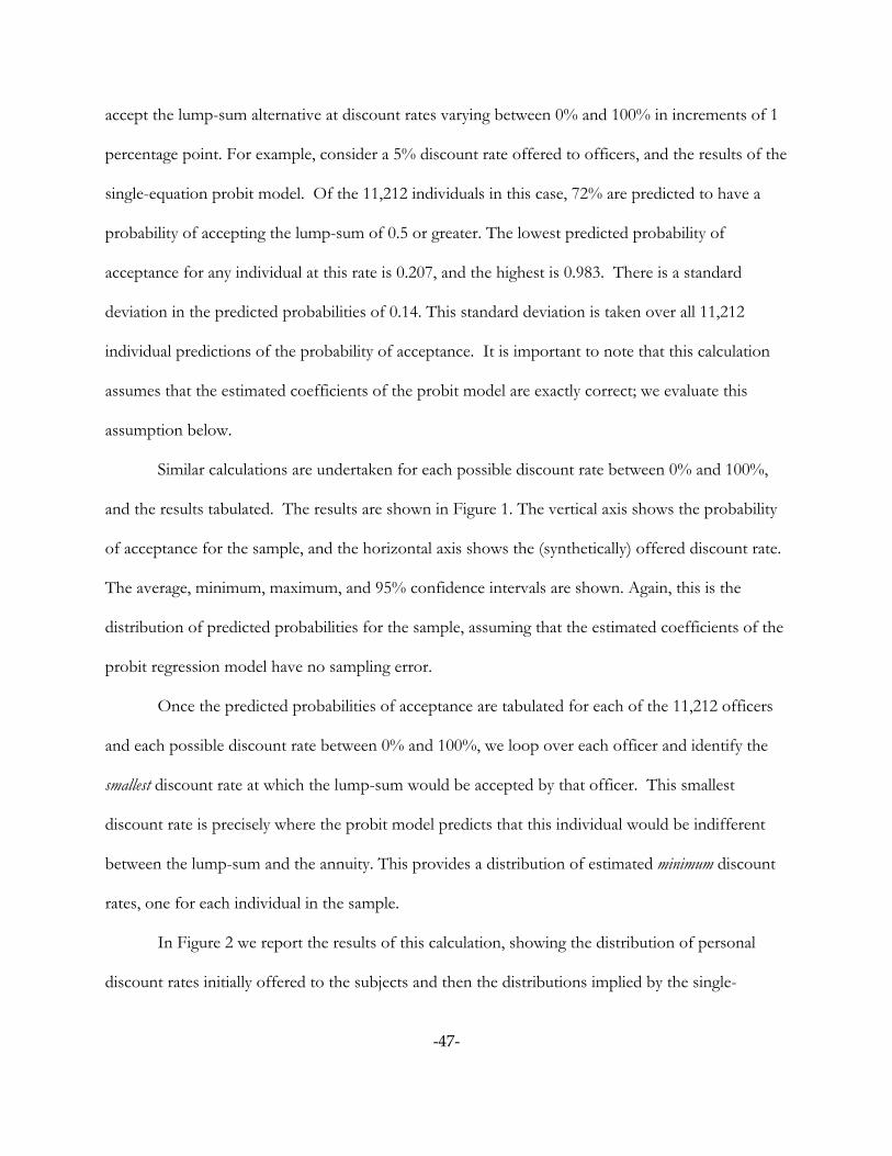
-47-
accept the lump-sum alternative at discount rates varying between 0% and 100% in increments of 1
percentage point. For example, consider a 5% discount rate offered to officers, and the results of the
single-equation probit model. Of the 11,212 individuals in this case, 72% are predicted to have a
probability of accepting the lump-sum of 0.5 or greater. The lowest predicted probability of
acceptance for any individual at this rate is 0.207, and the highest is 0.983. There is a standard
deviation in the predicted probabilities of 0.14. This standard deviation is taken over all 11,212
individual predictions of the probability of acceptance. It is important to note that this calculation
assumes that the estimated coefficients of the probit model are exactly correct; we evaluate this
assumption below.
Similar calculations are undertaken for each possible discount rate between 0% and 100%,
and the results tabulated. The results are shown in Figure 1. The vertical axis shows the probability
of acceptance for the sample, and the horizontal axis shows the (synthetically) offered discount rate.
The average, minimum, maximum, and 95% confidence intervals are shown. Again, this is the
distribution of predicted probabilities for the sample, assuming that the estimated coefficients of the
probit regression model have no sampling error.
Once the predicted probabilities of acceptance are tabulated for each of the 11,212 officers
and each possible discount rate between 0% and 100%, we loop over each officer and identify the
smallest discount rate at which the lump-sum would be accepted by that officer. This smallest
discount rate is precisely where the probit model predicts that this individual would be indifferent
between the lump-sum and the annuity. This provides a distribution of estimated minimum discount
rates, one for each individual in the sample.
In Figure 2 we report the results of this calculation, showing the distribution of personal
discount rates initially offered to the subjects and then the distributions implied by the single-

44 Virtually identical results are obtained with the model that corrects for possible sample-selection effects.
-48-
equation probit model used by WP.44 The left-hand side column of panels shows the results for all
separating personnel, the middle column of panels shows the results for separating officers, and the
right-hand side panels show the results for separating enlisted personnel. The top row of panels of
Figure 2 shows simply the after-tax discount rates that were offered, the middle row of panels shows
the discount rates inferred from the estimated “linear” model that allows discount rates to be
negative, and the bottom row of panels shows the discount rates inferred from the estimated “log-
linear” model that constrains discount rates to be positive. The horizontal axes in all charts are
identical, to allow simple visual comparisons.
The main result is that the distribution of estimated discount rates is much wider than the
distribution of offered rates. Indeed, for enlisted personnel the distribution of estimated rates is
almost entirely out-of-sample in comparison to the offered rates above it. There is nothing “wrong”
with these differences, although they will be critical when we calculate standard errors on these
estimated discount rates. Again, the estimated rates in the bottom charts of Figure 2 are based on the
logic of Figure 1: no prediction error is assumed from the estimated statistical model when it is
applied at the level of the individual to predict the threshold rate at which the lump-sum would be
accepted.
The second point to see from Figure 2 is that the distribution of estimated rates for officers
is generally much lower than the distribution for enlisted personnel, and has a much smaller variance.

-49-
Prob
abilit
y U
sing
Sin
gle
Equa
tion
Prob
it M
odel
Figu
re 1
: Pro
babi
lity
of A
ccep
tanc
e if
No
Pred
ictio
n Er
ror
Perc
enta
ge D
isco
unt R
ate
for O
ffice
rs0
1020
3040
5060
7080
9010
0
0
.25.5.751

-50-
Figu
re 2
: Offe
red
and
Estim
ated
Dis
coun
t Rat
es
Prob
abilit
y
Af
ter-T
ax D
isco
unt R
ate
Offe
red
025
5075
100
0.2.4.6
Prob
abilit
y
Afte
r-Tax
Dis
coun
t Rat
e O
ffere
d to
Sep
arat
ing
Offi
cers
0
2550
7510
0
0.2.4.6
Prob
abilit
y
Afte
r-Tax
Dis
coun
t Rat
e O
ffere
d to
Sep
arat
ing
Enlis
ted
Pers
onne
l
025
5075
100
0.2.4.6
Prob
abilit
yAl
low
ing
Neg
ativ
e D
isco
unt R
ates
Estim
ated
Indi
vidu
al D
isco
unt R
ate
for A
ll Se
para
ting
0
2550
7510
0
0.1.2.3.4
Prob
abilit
yAl
low
ing
Neg
ativ
e D
isco
unt R
ates
Estim
ated
Indi
vidu
al D
isco
unt R
ate
for S
epar
atin
g O
ffice
rs
025
5075
100
0.1.2.3
Prob
abilit
yAl
low
ing
Neg
ativ
e D
isco
unt R
ates
Es
timat
ed In
divi
dual
Dis
coun
t Rat
e fo
r Sep
arat
ing
Enlis
ted
Pers
onne
l
025
5075
100
0.2.4
Prob
abilit
yO
nly
Posi
tive
Dis
coun
t Rat
es
Estim
ated
Indi
vidu
al D
isco
unt R
ate
for A
ll Se
para
ting
0
2550
7510
0
0
.05.1.15.2
Prob
abilit
yO
nly
Posi
tive
Dis
coun
t Rat
es
Estim
ated
Indi
vidu
al D
isco
unt R
ate
for S
epar
atin
g O
ffice
rs
025
5075
100
0.1.2.3.4
Prob
abilit
yO
nly
Posi
tive
Dis
coun
t Rat
es
Es
timat
ed In
divi
dual
Dis
coun
t Rat
e fo
r Sep
arat
ing
Enlis
ted
Pers
onne
l
025
5075
100
0
.05.1.15.2

-51-
The third point to see from Figure 2 is that the distribution of estimated discount rates for
the model that imposes the constraint that discount rates be positive is generally much further to the
right than the unconstrained distribution. This qualitative effect is what one would expect from such
a constraint, of course, but the important point is how quantitatively important it is. The effect for
enlisted personnel is particularly substantial, reflecting the general uncertainty of the estimates for
those individuals.
An Extension to Consider Uncertainty
The main conclusion of WP is contained in their Table 6, which lists estimates of the average
discount rates for various groups of their subjects. Using the model that imposes the a priori
restriction that discount rates be positive, they report that the average discount rate for officers was
18.7% and that it was 53.6% for enlisted personnel. What are the standard errors on these means?
There is reason to expect that they could be quite large, due to constraints on the scope of the
natural experiment.
Individuals were offered a choice between a lump-sum and an annuity. The before-tax
discount rate that just equated the present value of the two instruments ranged between 17.5% and
19.8%, which is a very narrow range of discount rates. The after-tax equivalent rates ranged from a
low of 14.5% up to 23.5% for those offered the separation option, but over 99% of the after-tax
rates were between 17.6% and 20.4%, as shown in Figure 3. Thus the above inferences about
average discount rates for enlisted personnel are “out of sample,” in the sense that they do not
reflect direct observation of responses at those rates of 53.6%, or indeed at any rates outside the

45 Relaxing the functional form also allows some additional uncertainty into the estimation of individualdiscount rates.
-52-
Fraction of Sample (N=293,388)
Figure 3: Percent After-Tax Discount Rates Offered
17 18 19 20 21 22 23 24
0
.05
.1
interval [14.5%, 23.5%]. Figure 2
illustrates this point as well. The
average for enlisted personnel
therefore reflects, and relies on, the
predictive power of the parametric
functional forms fitted to the observed
data. The same general point is true for
officers, but the problem is far less severe, as the relatively narrow range of the distribution for
officers in Figure 2 demonstrates.
Even if one accepted the parametric functional forms (probit), the standard errors of
predictions outside of the sample range of break-even discount rates will be much larger than those
within the sample range.45 The standard errors of the predicted response can be calculated directly
from the estimated model. Note that this is not the same as the distributions shown in Figures 1 and
2, which are distributions over the sample of individuals at each simulated discount rate that assume
that the model provides a perfect prediction for each individual. In other words, the predictions underlying
Figures 1 and 2 just use the average prediction for each individual as the truth, so the sampling error
reflected in the distributions only reflects sampling over the individuals. One can generate standard
errors that also capture the uncertainty in the probit model coefficients as well.
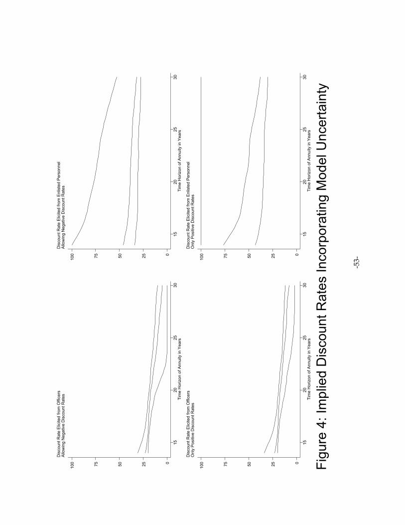
-53-
Figu
re 4
: Im
plie
d D
isco
unt R
ates
Inco
rpor
atin
g M
odel
Unc
erta
inty
Dis
coun
t Rat
e El
icite
d fro
m O
ffice
rsAl
low
ing
Neg
ativ
e D
isco
unt R
ates Tim
e H
oriz
on o
f Ann
uity
in Y
ears
1520
2530
0255075100
Dis
coun
t Rat
e El
icite
d fro
m E
nlis
ted
Pers
onne
lAl
low
ing
Neg
ativ
e D
isco
unt R
ates Tim
e H
oriz
on o
f Ann
uity
in Y
ears
1520
2530
0255075100
Dis
coun
t Rat
e El
icite
d fro
m O
ffice
rsO
nly
Posi
tive
Dis
coun
t Rat
es
Tim
e H
oriz
on o
f Ann
uity
in Y
ears
1520
2530
0255075100
Dis
coun
t Rat
e El
icite
d fro
m E
nlis
ted
Pers
onne
lO
nly
Posi
tive
Dis
coun
t Rat
es
Tim
e H
oriz
on o
f Ann
uity
in Y
ears
1520
2530
0255075100

46 The time horizon of the annuity offered to individuals in the field varied directly with the years of militaryservice completed. For each year of service the horizon on the annuity was 2 years longer. As a result, the annuitiesbeing considered by individuals were between 14 and 30 years in length. With roughly 10% of the sample at eachhorizon, the average annuity horizon was around 22 years.
47 In fact, we calculate rates only up to 100%, so the upper confidence intervals for the log-linear model(bottom right panel in Figure 4) is constrained to equal 100% for that reason. It would be a simple matter to allow thecalculation to consider higher rates, but little inferential value in doing so.
48 It is a standard result from elementary econometrics that the forecast interval widens as one uses theregression model to predict for values of the exogenous variables that are further and further away from their average(e.g., Greene [1993; p.164-166]). Figure 5 provides a textbook illustration of that result.
-54-
Figure 4 displays the results of taking into account the uncertainty about the coefficients of
the estimated model used by WP. Since it is an important dimension to consider, we show the time
horizon for the elicited discount rates on the horizontal axis.46 The middle line shows a cubic spline
through the predicted average discount rate. The top (bottom) line shows a cubic spline through the
upper (lower) bound of the 95% confidence interval, allowing for uncertainty in the individual
predictions due to reliance on an estimated statistical model to infer discount rates.47 Thus, in Figure
4 we see that there is considerable uncertainty about the discount rates for enlisted personnel, and
that it is asymmetric. On balance, the model implies a considerable skewness in the distribution of
rates for enlisted personnel, with some individuals having extremely high implied discount rates.
Turning to the results for officers, we find much less of an effect from model uncertainty. In this
case the rates are relatively precisely inferred, particularly around the range of rates spanning the
effective rates offered, as one would expect.48
We conclude that the results for enlisted personnel are too imprecisely estimated for them to be used to draw
reliable inferences about the discount rates. However, the results for officers are relatively tightly estimated, and can be
used to draw more reliable inferences. The reason for the lack of precision in the estimates for enlisted
personnel is transparent from Figure 2: the estimates rely on out-of-sample predictions, and the
standard errors embodied in Figure 4 properly reflect the uncertainty of such an inference.
49 See Ferber and Hirsch [1978][1982] and Hausman and Wise [1985] for wonderful reviews.
-55-
9. Social Experiments
A. What Constitutes a Social Experiment in Economics?
Ferber and Hirsch [1982; p.7] define social experiments in economics as “.... a publicly
funded study that incorporates a rigorous statistical design and whose experimental aspects are
applied over a period of time to one or more segments of a human population, with the aim of
evaluating the aggregate economic and social effects of the experimental treatments.” In many
respects this definition includes field experiments and even lab experiments. The point of departure
for social experiments seems to be that they are a part of a government agency’s attempt to evaluate
programs by deliberate variations in agency policies. Thus they typically involve variations in the
way that the agency does its normal business, rather than de novo programs. This characterization fits
well with the tradition of large-scale social experiments in the 1960s and 1970s, dealing with negative
income taxes, employment programs, health insurance, electricity pricing, and housing allowances.49
In recent years the lines have been blurred. Government agencies have been using
experiments to examine issues or policies that have no close counterpart, so that their use cannot be
viewed as variations on a bureaucratic theme. Perhaps the most notable social experiments in recent
years have been paired-audit experiments to identify and measure discrimination. These involve the
use of “matched pairs” of individuals, who are made to look as much alike as possible apart from
the protected characteristics (e.g., race). These pairs then confront the target subjects, which are
employers, landlords, mortgage loan officers, or car salesmen. The majority of audit studies
conducted to date have been in the fields of employment discrimination and housing discrimination
(see Riach and Rich [2002] for a review).
The lines have also been blurred by open lobbying efforts by private companies to influence

50 For example, the Department of Housing and Urban Development has funded three national paired-auditstudies of discrimination in urban housing markets, the 1977 Housing Market Practices Study, the 1989 HousingDiscrimination Study, and the 2000 Housing Discrimination Study. The data from the first study appear to be lost, andthe data for the latter studies is projected to be available for the public in mid-2003, well after the immediate policyimpact of the studies. Most of the studies collected in Sunstein et al. [2002] have been previously published in academiclaw journals, and thank the U.S. National Science Foundation (p. ix) for support; the authors of the various studiesdecline to make their data available.
-56-
social policy change by means of experiments. Exxon funded a series of experiments and surveys,
collected by Hausman [1993], to ridicule the use of the contingent valuation method in
environmental damage assessment. This effort was in response to the role that such surveys
potentially played in the criminal action brought by government trustees after the Exxon Valdez oil
spill. Similarly, ExxonMobil funded a series of experiments and focus groups, collected in Sunstein,
Hastie, Payne, Schkade and Viscusi [2002], to ridicule the way in which juries determine punitive
damages. This effort was in response to the role that juries played in determining punitive damages
in the civil lawsuits generated by the Exxon Valdez oil spill. It is also playing a major role in ongoing
efforts by some corporations to effect “tort reform” with respect to limiting appeal bonds for
punitive awards and even caps on punitive awards.
One feature of the use of experiments to measure discrimination, and the use of experiments
to influence policy and legal rulings, is that the data underlying the experiments is almost never made
available for review by potential critics. This is true despite the use of government funds to
undertake the research,50 and despite the research being published in peer-reviewed academic
journals of note. Heckman and Smith [1995; p.94] draw the implication for the scientific process:
A final argument offered in favor of experiments is that they produce “one number”rather than the bewildering array of nonexperimental estimates often found in theliterature on program evaluation. In assessing the argument, it is important todistinguish the consensus produced by monopoly from the consensus that emergesfrom scholarship. Many organizations producing experimental analyses have beenunwilling to share their data with the academic research community. The appearanceof a consensus view is a consequence of only one interpretation of the data beinggiven.
-57-
This point is obviously of more general relevance for experimental research in the lab and field.
B. Methodological Lessons
The literature on social experiments has been the subject of sustained methodological
criticism, all of which appears to have been ignored by proponents of the method. Unfortunately,
this neglect has created a false tension between the use of experiments and the use of econometrics
applied to field data. We believe that virtually all of the criticisms of social experiments potentially
apply in some form to field experiments unless they are run in an ideal manner, so we briefly review
the important ones. Indeed, many of them also apply to conventional lab experiments.
Recruitment and the Evaluation Problem
Heckman and Smith [1995; p.87] go to the heart of the role of experiments in a social policy
setting, when they note that “The strongest argument in favor of experiments is that under certain
conditions they solve the fundamental evaluation problem that arises from the impossibility of
observing what would happen to a given person in both the state where he or she receives a
treatment (or participates in a program) and the state where he or she does not. If a person could be
observed in both states, the impact of the treatment on that person could be calculated by
comparing his or her outcomes in the two states, and the evaluation problem would be solved.”
Randomization to treatment is the means by which social experiments solve this problem if one
assumes that the act of randomizing subjects to treatment does not lead to a classic sample selection
effect, which is to say that it does not “alter the pool of participants of their behavior” (p.88).
Unfortunately, randomization could plausibly lead to either of these outcomes, which are not
fatal but do necessitate the use of “econometric(k)s.” We have discussed already the possibility that
-58-
the use of randomization could attract subjects to experiments that are less risk averse than the
population, if the subjects rationally anticipate the use of randomization. It is well known in the
field of clinical drug trials that persuading patients to participate in randomized studies is much
harder than persuading them to participate in non-randomized studies (e..g., Kramer and Shapiro
[1984]). The same problem applies to social experiments, as evidenced by the difficulties that can be
encountered when recruiting decentralized bureaucracies to administer the random treatment (e.g.,
Hotz [1992]). Heckman and Robb [1985] note that the refusal rate in one randomized job training
program was over 90%, with many of the refusals citing ethical concerns with administering a
random treatment.
What relevance does this have for field or lab experiments? The answer is simple: we do not
know, since it has not been systematically studied. On the other hand, field experiments have one
major advantage if they involve the use of subjects in their natural environment, undertaking tasks
that they are familiar with, since no sample selection is involved at the first level of the experiment.
In conventional lab experiments there is sample selection at two stages: the decision to attend
college, and then the decision to be in the experiment. In synthetic field experiments, as we defined
the term in section 1, the subject selects to be in the naturally occurring market and then in the
decision to be in the experiment. So the synthetic field experiment shares this two-stage selection
process with conventional lab experiments. However, the natural field experiment has only one
source of possible selection bias: the decision to be in the naturally occurring market. Hence the
bookies that accepted the contrived bets of Camerer [1998] had no idea that he was conducting an
experiment, and did not select “for” the transaction with the experimenter. Of course, they were
bookies, and hence had selected for that occupation.
A variant on the recruitment problem occurs in settings where subjects are observed over a

-59-
period of time, and attrition is a possibility. Statistical methods can be developed to use differential
attrition rates as valuable information on how subjects value outcomes (e.g., see Philipson and
Hedges [1998]).
Substitution and the Evaluation Problem
The second assumption underlying the validity of social experiments is that “close
substitutes for the experimental treatment are not readily available” (Heckman and Smith [1995;
p.88]). If they are, then subjects who are placed in the control group could opt for the substitutes
available outside the experimental setting. The result is that outcomes in the control no longer show
the effect of “no treatment,” but instead the effect of “possible access to an uncontrolled
treatment.” Again, this is not a fatal problem, but one that has to be addressed explicitly. In fact, it
has arisen already in the elicitation of preferences over field commodities, as discussed in section 4.
Experimenter Effects
In social experiments, given the open nature of the political process, it is almost impossible
to hide the experimental objective from the person implementing the experiment or the subject.
The paired-audit experiments are perhaps the most obvious targets of this, since the “treatments”
themselves have any number of ways to bring about the conclusion that is favored by the research
team conducting the experiment. In this instance, the Urban Institute makes no bones about its
view that discrimination is a widespread problem and that paired-audit experiments are a critical way
to address it (e.g., a casual perusal of Fix and Struyk [1993]). There is nothing wrong with this at all,
apart from the fact that it is hard to imagine how volunteer auditors would not see things similarly.
Indeed, Heckman [1998; p.104] notes that “auditors are sometimes instructed on the ‘problem of

-60-
discrimination in American Society’ prior to sampling firms, so they may have been coached to find
what audit agencies wanted them to find.” The opportunity for unobservables to influence the
outcome are rampant here.
Of course, simple controls could be designed to address this issue. One could have different
test-pairs visit multiple locations, to help identify the effect of a given pair on the overall measure of
discrimination. The variability of measured discrimination across audit pairs is marked, and raises
statistical issues as well as issues of interpretation (e.g., see Heckman and Siegelman [1993]).
Another control could be to have an artificial location for the audit pair to visit, where their
“unobservables” could be “observed” and controlled for in later statistical analyses. This procedure
is used in a standard manner in private business concerned with measuring the quality of customer
relations in the field.
One stunning example of experimenter effects from Bohm [1984b] illustrates what can
happen when the subjects see a meta-game beyond the experiment itself. In 1980 he undertook a
field experiment for a local government in Stockholm that was considering expanding a bus route to
a major hospital and a factory. The experiment was to elicit valuations from people who were
naturally affected by this route, to see if their aggregate contributions would make it worthwhile to
provide the service. A key feature of the experiment was that the subjects would have to be willing
to pay for the public good if it was to be provided for a trial period of 6 months. Everyone who was
likely to contribute was given information on the experiment, but when it came time for the
experiment virtually nobody turned up! The reason was that the local trade unions had decided to
boycott the experiment, since it represented a threat to the current way in which such services were
provided. The union leaders expressed their concerns, summarized by Bohm [1984b; p.136] as
follows:

51 It is a pity that Bohm [1984b] himself firmly categorized this experiment as a failure, although one canunderstand that perspective.
52 See Philipson and Hedges [1998] for a general statistical perspective on this problem.
-61-
They reported that they had held meetings of their own and had decided (1) that theydid not accept the local government’s decision not to provide them with regular busservice on regular terms; (2) that they did not accept the idea of having to pay in away that differs from the way that “everybody else” pays (bus service is subsidized inthe area) – the implication being that they would rather go without this bus service,even if their members felt it would be worth the costs; (3) that they would not like tohelp in realizing an arrangement that might reduce the level of public servicesprovided free or at low costs. It was argued that such an arrangement, if acceptedhere, could spread to other parts of the public sector; and (4) on these grounds, theyadvised their union members to abstain from participating in the project.
This fascinating outcome is actually more relevant for experimental economics in general than it
might seem.51
When certain institutions are imposed on subjects, and certain outcomes tabulated, it does
not follow that the outcomes of interest for the experimenter are the ones that are of interest to the
subject.52 For example, Isaac and Smith [1985] observe virtually no instances of predatory pricing in
a partial equilibrium market in which the prey had no alternative market to escape to at the first taste
of blood. In a comparable multi-market setting in which subjects could choose to exit markets for
other markets, Harrison [1988] observed many instances of predatory pricing.

-62-
10. Conclusion
We have avoided drawing a single, bright line between field experiments and lab
experiments. One reason is that there are several dimensions to that line, and inevitably there will be
some trade-offs between those. The extent of those trade-offs will depend on where researchers fall
in terms of their agreement with the argument and issues we raise.
Another reason is that we disagree where the line would be drawn. One of us (Harrison),
bred in the barren test-tube setting of classroom labs sans ferns, sees virtually any effort to get out of
the classroom as constituting a field experiment to some useful degree. The other (List), raised in the
wilds amidst naturally occurring sportscard geeks, would include only those experiments that used
free-range subjects. Despite this disagreement on the boundaries between one category of
experiments and another category, however, we agree on the characteristics that make a field
experiment differ from a lab experiment.
The main conclusion we draw is that experimenters should be wary of the conventional
wisdom that abstract, imposed treatments allow general inferences. In an attempt to ensure
generality and control by gutting all instructions and procedures of field referents, the traditional lab
experimenter has arguably lost control to the extent that subjects seek to provide their own field
referents. The obvious solution is to conduct experiments both ways: with and without naturally
occurring field referents and context. If there is a difference, then it should be studied. If there is no
difference, one can conditionally conclude that the field behavior in that context travels to the lab
environment.

-63-
References
Bateman, Ian; Munro, Alistair; Rhodes, Bruce; Starmer, Chris, and Sugden, Robert, “Does Part-Whole Bias Exist? An Experimental Investigation,” Economic Journal, 107, March 1997, 322-332.
Behrman, Jere R.; Rosenzweig, Mark R.,, and Taubman, Paul, “Endowments and the Allocation ofSchooling in the Family and in the Marriage Market: The Twins Experiment,” Journal ofPolitical Economy, 102(6), December 1994, 1131-1174.
Berlin, Brent, and Kay, Paul, Basic Color Terms: Their Universality and Evolution (Berkeley: University ofCalifornia Press, 1969).
Binswanger, Hans P., “Attitudes Toward Risk: Experimental Measurement in Rural India,” AmericanJournal of Agricultural Economics, 62, August 1980, 395-407.
Binswanger, Hans P., “Attitudes Toward Risk: Theoretical Implications of an Experiment in RuralIndia,” Economic Journal, 91, December 1981, 867-890.
Blackburn, McKinley; Harrison, Glenn W., and Rutström, E. Elisabet, “Statistical Bias Functionsand Informative Hypothetical Surveys,” American Journal of Agricultural Economics, 76(5),December 1994, 1084-1088.
Bohm, Peter, “Estimating the Demand for Public Goods: An Experiment,” European EconomicReview, 3, June 1972, 111-130.
Bohm, Peter, “Estimating Willingness to Pay: Why and How?,” Scandinavian Journal of Economics,LXXXI, 1979, 142-153.
Bohm, Peter, “Revealing Demand for an Actual Public Good,” Journal of Public Economics, 24, 1984a,135-151.
Bohm, Peter, “Are There Practicable Demand-Revealing Mechanisms?” in H. Hanusch (ed.), PublicFinance and the Quest for Efficiency (Detroit: Wayne State University Press, 1984b).
Bohm, Peter, “Behavior Under Uncertainty Without Preference Reversal: A Field Experiment,” in J.Hey (ed.), Experimental Economics (Heidelberg: Physica-Verlag, 1994).
Bohm, Peter, and Lind, Hans, “Preference Reversal, Real-World Lotteries, and Lottery-InterestedSubjects,” Journal of Economic Behavior and Organization, 22, 1993, 327-348.
Botelho, Anabela; Harrison, Glenn W.; Hirsch, Marc A., and Rutström, Elisabet E., “BargainingBehavior, Demographics and Nationality: What Can the Experimental Evidence Show?”Economics Working Paper, Moore School of Business, University of South Carolina, 2002; http://dmsweb.moore.sc.edu/glenn/wp/.

-64-
Bronars, Stephen G., and Grogger, Jeff, “The Economic Consequences of Unwed Motherhood:Using Twin Births as a Natural Experiment,” American Economic Review, 84(5), December1994, 1141-1156.
Burns, Penny, “Experience and Decision Making: A Comparison of Students and Businessmen in aSimulated Progressive Auction,” in V.L. Smith (ed.), Research in Experimental Economics(Greenwich, CT: JAI Press, 1985, volume 3).
Camerer, Colin F., “Can Asset Markets Be Manipulated? A Field Experiment with RacetrackBetting,” Journal of Political Economy, 106(3), 1998, 457-482.
Cameron, Lisa A., “Raising The Stakes in the Ultimatum Game: Experimental Evidence fromIndonesia,” Economic Inquiry, 37(1), January 1999, 47-59.
Carson, Richard T.; Mitchell, Robert C.; Hanemann, W. Michael; Kopp, Raymond J.; Presser,Stanley; and Ruud, Paul A., A Contingent Valuation Study of Lost Passive Use Values ResultingFrom the Exxon Valdez Oil Spill (Anchorage: Attorney General of the State of Alaska,November 1992).
Carson, Richard T.; Mitchell, Robert C.; Hanemann, W. Michael; Kopp, Raymond J.; Presser,Stanley; and Ruud, Paul A., “Contingent Valuation and Lost Passive Use: Damages from theExxon Valdez”, Discussion Paper 94-18, Resources for the Future, Washington, DC, March1994.
Coller, Maribeth, and Williams, Melonie B., “Eliciting Individual Discount Rates,” ExperimentalEconomics, 2, 1999, 107-127.
Conlisk, John, “Three Variants on the Allais Example,” American Economic Review, 79(3), June 1989,392-407.
Conlisk, John, “Why Bounded Rationality?” Journal of Economic Literature, 34, June 1996, 669-700.
Cubitt, Robin P., and Sugden, Robert, “On Money Pumps,” Games and Economic Behavior, 37, 2001,121-160.
Cummings, Ronald G., and Harrison, Glenn W., “Was the Ohio Court Well Informed in TheirAssessment of the Accuracy of the Contingent Valuation Method?,” Natural Resources Journal,34(1), Winter 1994, 1-36.
Cummings, Ronald G.; Harrison, Glenn W., and Osborne, Laura L., “Can the Bias of ContingentValuation Be Reduced? Evidence from the Laboratory,” Economics Working Paper B-95-03,Division of Research, College of Business Administration, University of South Carolina,1995; http://dmsweb.moore.sc.edu/glenn/wp/.
Cummings, Ronald G.; Harrison, Glenn W., and Rutström, E. Elisabet, “Homegrown Values andHypothetical Surveys: Is the Dichotomous Choice Approach Incentive Compatible?”

-65-
American Economic Review, 85(1), March 1995, 260-266.
Cummings, Ronald G. and Taylor, Laura O., “Unbiased Value Estimates for Environmental Goods:A Cheap Talk Design for the Contingent Valuation Method,” American Economic Review,89(3), June 1999, 649-665.
Davis, Douglas D., and Holt, Charles A., Experimental Economics (Princeton, NJ: Princeton UniversityPress, 1993).
Deacon, Robert T., and Sonstelie, Jon, “Rationing by Waiting and the Value of Time: Results from aNatural Experiment,” Journal of Political Economy, 93(4), August 1985, 627-647.
Duddy, Edward A., “Report on an Experiment in Teaching Method,” Journal of Political Economy,32(5), October 1924, 582-603.
Dyer, Douglas, and Kagel, John H., “Bidding in Common Value Auctions: How the CommercialConstruction Industry Corrects for the Winner’s Curse,” Management Science, 42(10), October1996, 1463-1475.
Dyer, Douglas; Kagel, John H., and Levin, Dan, “A Comparison of Naive and Experienced Biddersin Common Value Offer Auctions: A Laboratory Analysis,” Economic Journal, 99, 1989, 108-115.
Fan, Chinn-Ping, “Allais Paradox In the Small,” Journal of Economic Behavior and Organization, 49(3),November 2002, 411-421.
Ferber, Robert, and Hirsch, Werner Z., “Social Experimentation and Economic Policy: A Survey,” Journal of Economic Literature, 16(4), December 1978, 1379-1414.
Ferber, Robert, and Hirsch, Werner Z., Social Experimentation and Economic Policy (New York:Cambridge University Press, 1982).
Fix, Michael, and Struyk, Raymond J. (eds.), Clear and Convincing Evidence: Measurement of Discriminationin America (Washington, DC: The Urban Institute Press, 1993).
Forsythe, Robert; Nelson, Forrest; Neumann, George R., and Wright, Jack, “Anatomy of anExperimental Political Stock Market,” American Economic Review, 82, December 1992, 1142-1161.
Frech, H.E., “The Property Rights Theory of the Firm: Empirical Results from a NaturalExperiment,” Journal of Political Economy, 84(1), February 1976, 143-152.
Frederick, Shane; Loewenstein, George; and O’Donoghue, Ted, “Time Discounting and TimePreference: A Critical Review,” Journal of Economic Literature, XL, June 2002, 351-401.
Gigerenzer, Gerd; Todd, Peter M., and the ABC Research Group, Simple Heuristics That Make Us

-66-
Smart (New York: Oxford University Press, 2000).
Gimotty, Phyllis A., “Delivery of preventive health services for breast cancer control: A longitudinalview of a randomized controlled trial,” Health Services Research, 37(1), February 2002.
Greene, William H., Econometric Analysis (New York: Macmillan, Second Edition, 1993).
Greene, William H., LIMDEP Version 7.0 User’s Manual (Bellport, NY: Econometric Software, Inc.,1995).
Grether, David M.; Isaac, R. Mark, and Plott, Charles R., “The Allocation of Landing Rights byUnanimity among Competitors,” American Economic Review (Papers & Proceedings), 71, May1981, 166-171.
Grether, David M.; Isaac, R. Mark, and Plott, Charles R., The Allocation of Scarce Resources:Experimental Economics and the Problem of Allocating Airport Slots (Boulder: Westview Press,1989).
Grether David M., and Plott, Charles R., “The Effects of Market Practices in Oligopolistic Markets:An Experimental Examination of the Ethyl Case,” Economic Inquiry, 22, October 1984,479-507.
Harrison, Glenn W., “Predatory Pricing in A Multiple Market Experiment,” Journal of EconomicBehavior and Organization, 9, 1988, 405-417.
Harrison, Glenn W., “Theory and Misbehavior of First-Price Auctions: Reply,” American EconomicReview, 82, December 1992a, 1426-1443.
Harrison, Glenn W., “Market Dynamics, Programmed Traders, and Futures Markets: Beginning theLaboratory Search for a Smoking Gun,” Economic Record, 68, 1992b (Special Issue on FuturesMarkets), 46-62.
Harrison, Glenn W., Harstad, Ronald M., and Rutström, E. Elisabet, “Experimental Methods andElicitation of Values,” Unpublished Manuscript, Department of Economics, Moore School ofBusiness, University of South Carolina, 2003; http://dmsweb.moore.sc.edu/glenn/wp/.
Harrison, Glenn W.; Johnson, Eric; McInnes, Melayne M.; and Rutström, E. Elisabet, “IndividualChoice in the Laboratory: Paradox Reloaded,” Unpublished Manuscript, Department ofEconomics, Moore School of Business, University of South Carolina, 2003;http://dmsweb.moore.sc.edu/glenn/wp/.
Harrison, Glenn W.; Lau, Morten Igel, and Williams, Melonie B., “Estimating Individual DiscountRates for Denmark: A Field Experiment,” American Economic Review, 92(5), December 2002,1606-1617
Harrison, Glenn W., and Lesley, James C., “Must Contingent Valuation Surveys Cost So Much?”

-67-
Journal of Environmental Economics and Management, 31, June 1996, 79-95.
Harrison, Glenn W., and List, John A., “Naturally Occurring Markets and Exogenous LaboratoryExperiments: A Case Study of the Winner’s Curse,” Unpublished Manuscript, Department ofEconomics, Moore School of Business, University of South Carolina, 2003;http://dmsweb.moore.sc.edu/glenn/wp/.
Harrison, Glenn W., and Rutström, Elisabet, “Doing It Both Ways -- Experimental Practice andHeuristic Context,” Behavioral and Brain Sciences, 24(3), June 2001, 413-414.
Harrison, Glenn W., and Rutström, Elisabet, “Do Higher Stakes Change Behavior in UltimatumGames?” Unpublished Manuscript, Department of Economics, Moore School of Business,University of South Carolina, January 2002.
Hausman, Jerry A., Contingent Valuation (New York: North-Holland, 1993).
Hausman, Jerry A., and Wise, David A., Social Experimentation (Chicago: University of Chicago Press,1985).
Hayes, J.R., and Simon, H.A., “Understanding Written Problem Instructions,” in L.W. Gregg (ed.),Knowledge and Cognition (Hillsdale, NJ: Erlbaum, 1974).
Heckman, James J., “Detecting Discrimination,” Journal of Economic Perspectives, 12(2), Spring 1998,101-116.
Heckman, James J., and Robb, Richard, “Alternative Methods for Evaluating the Impact ofInterventions,” in J. Heckman and B. Singer (eds.), Longitudinal Analysis of Labor Market Data(New York: Cambridge University Press, 1985).
Heckman, James J., and Siegelman, Peter, “The Urban Institute Audit Studies: Their Methods andFindings,” in M. Fix and R.J. Struyk, (eds), Clear and Convincing Evidence: Measurement ofDiscrimination in America (Washington, DC: The Urban Institute Press, 1993).
Heckman, James J., and Smith, Jeffrey A., “Assessing the Case for Social Experiments,” Journal ofEconomic Perspectives, 9(2), Spring 1995, 85-110.
Henrich, Joseph, and McElreath, Richard, “Are Peasants Risk-Averse Decision Makers?” CurrentAnthropology, 43(1), February 2002, 172-181.
Hoffman, Elizabeth; McCabe, Kevin A., and Smith, Vernon L., “On Expectations and the MonetaryStakes in Ultimatum Games,” International Journal of Game Theory, 25(3), 1996, 289-301.
Holt, Charles A., and Laury, Susan K., “Risk Aversion and Incentive Effects,” American EconomicReview, 92(5), December 2002, 1644-1655.
Hong, James T., and Plott, Charles R., “Rate Filing Policies for Inland Water Transportation: An

-68-
Experimental Approach,” Bell Journal of Economics, 13, Spring 1982, 1-19.
Hotz, V. Joseph, “Designing an Evaluation of JTPA,”, in C. Manski and I. Garfinkel (eds.),Evaluating Welfare and Training Programs (Cambridge: Harvard University Press, 1992).
Hoxby, Caroline M., “The Effects of Class Size on Student Achievement: New Evidence FromPopulation Variation,” Quarterly Journal of Economics, November 2000, 1239-1285.
Isaac, R. Mark, and Smith, Vernon L., “In Search of Predatory Pricing,” Journal of Political Economy,93, April 1985, 320-345.
Kachelmeier, Steven J., and Shehata, Mohamed, “Examining Risk Preferences Under HighMonetary Incentives: Experimental Evidence from the People’s Republic of China,”American Economic Review, 82(5), December 1992, 1120-1141.
Kagel, John H.; Battalio, Raymond C., and Walker, James M., “Volunteer Artifacts in Experimentsin Economics: Specification of the Problem and Some Initial Data from a Small-Scale FieldExperiment,” in V.L. Smith (ed.), Research in Experimental Economics (Greenwich, CT: JAIPress, 1979, volume 1).
Kagel, John H.; Harstad, Ronald M., and Levin, Dan, “Information Impact and Allocation Rules inAuctions with Affiliated Private Values: A Laboratory Study,” Econometrica, 55, November1987, 1275-1304.
Kagel, John H., and Levin, Dan, “The Winner’s Curse and Public Information in Common ValueAuctions,” American Economic Review, 76, December 1986, 894-920.
Kagel, John H., and Levin, Dan, “Common Value Auctions With Insider Information,” Econometrica,67(5), September 1999, 1219-1238.
Kagel, John H., and Levin, Dan, Common Value Auctions and the Winner’s Curse (Princeton: PrincetonUniversity Press, 2002).
Kramer, Michael, and Shapiro, Stanley, “Scientific Challenges in the Application of RandomizedTrials,” Journal of the American Statistical Association, 252, November 16, 1984, 2739-2745.
Kunce, Mitch; Gerking, Shelby, and Morgan, William, “Effects of Environmental and Land UseRegulation in the Oil and Gas Industry Using the Wyoming Checkerboard as anExperimental Design,” American Economic Review, 92(5), December 2002, 1588-1593.
Levine, Michael E., and Plott, Charles R., “Agenda Influence and Its Implications,” Virginia LawReview, 63, May 1977, 561-604.
Lichtenstein, Sarah, and Slovic, Paul, “Response-Induced Reversals of Gambling: An ExtendedReplication in Las Vegas,” Journal of Experimental Psychology, 101, 1973, 16-20.

-69-
List, John A., “Do Explicit Warnings Eliminate the Hypothetical Bias in Elicitation Procedures?Evidence from Field Auctions for Sportscards,” American Economic Review, 91(4), December2001, 1498-1507.
List, John, and Cherry, Todd, “Learning to Accept in Ultimatum Games: Evidence from anExperimental Design that Generates Low Offers,” Experimental Economics, 3(1), 2000, 11-29.
List, John A., and Lucking-Reiley, David, “The Effects of Seed Money and Refunds on CharitableGiving: Experimental Evidence from a University Capital Campaign,” Journal of PoliticalEconomy, 110(1), 2002, 215-233.
List, John, and Shogren, Jason, “Price Signals and Bidding Behavior in Second-Price Auctions withRepeated Trials,” American Journal of Agricultural Economics, 81, November 1999, 942-929..
Machina, Mark J., “Dynamic Consistency and Non-Expected Utility Models of Choice UnderUncertainty,” Journal of Economic Literature, XXVII, December 1989, 1622-1668.
McClennan, Edward F., Rationality and Dynamic Choice (New York: Cambridge University Press,1990).
McDaniel, Tanga M., and E. Elisabet Rutström, “Decision Making Costs and Problem SolvingPerformance,” Experimental Economics, 4(2), October 2001, 145-161.
Metrick, Andrew, “A Natural Experiment in ‘Jeopardy!’, “ American Economic Review, 85(1), March1995, 240-253.
Meyer, Bruce D.; Viscusi, W. Kip, and Durbin, David L., “Workers’ Compensation and InjuryDuration: Evidence from a Natural Experiment,” American Economic Review, 85(3), June 1995,322-340.
Milgrom, Paul R. and Robert J. Weber, “A Theory of Auctions and Competitive Bidding,”Econometrica, 50(5), September 1982, 1089-1122.
Mitchell, Robert C., and Carson, Richard T., Using Surveys to Value Public Goods: The ContingentValuation Method (Baltimore: Johns Hopkins Press, 1989).
Pearl, Judea, Heuristics: Intelligent Search Strategies for Computer Problem Solving (Reading, MA: Addison-Wesley, 1984).
Philipson, Tomas, and Hedges, Larry V., “Subject Evaluation in Social Experiments,” Econometrica,66(2), March 1998, 381-408.
Plott, Charles R., and Levine, Michael E., “A Model of Agenda Influence on Committee Decisions,”American Economic Review, 68(1), March 1978, 146-160.
Riach, P.A. and J. Rich, “Field Experiments of Discrimination in the Market Place,” Economic Journal,

-70-
112, November, 2002, F480-F518.
Rosenthal, R., and Jacobson, L., Pygmalion in the Classroom (New York: Holt, Rhinehart & Winston,1968).
Roth, Alvin E., “A Natural Experiment in the Organization of Entry-Level Labor Markets: RegionalMarkets for New Physicians and Surgeons in the United Kingdom,” American EconomicReview, 81(3), June 1991, 415-440.
Rutström, E. Elisabet, “Home-Grown Values and the Design of Incentive Compatible Auctions,”International Journal of Game Theory, 27(3), 1998, 427-441.
Slonim, Robert, and Roth, Alvin E., “Learning in High Stakes Ultimatum Games: An Experiment inthe Slovak Republic,” Econometrica, 66(3), May 1998, 569-596.
Smith, Vernon L., “An Experimental Study of Competitive Market Behavior,” Journal of PoliticalEconomy, 70, 1962, 111-137.
Smith, Vernon L., “Microeconomic Systems As An Experimental Science,” American Economic Review,72(5), December 1982, 923-955.
Smith, Vernon L., “Rational Choice: The Contrast Between Economics and Psychology,” Journal ofPolitical Economy, 99, August 1991, 877-897.
Smith, Vernon L.; Suchanek, G.L., and Williams, Arlington W., “Bubbles, Crashes, and EndogenousExpectations in Experimental Spot Asset Markets,” Econometrica, 56, 1988, 1119-1152.
Sunstein, Cass R.,; Hastie, Reid; Payne, John W.; Schkade, David A., and Viscusi, W. Kip, PunitiveDamages: How Juries Decide (Chicago: University of Chicago Press, 2002).
Warner, John T., and Pleeter, Saul, “The Personal Discount Rate: Evidence from MilitaryDownsizing Programs,” American Economic Review, 91(1), March 2001, 33-53.
Wierzbicka, Anna, Semantics: Primes and Universals (New York: Oxford University Press, 1996).