What Characterizes a Shadow Boundary under the Sun and Sky?

Xiang Huang�∗, Gang Hua�, Jack Tumblin�, Lance Williams�

�EECS Dept. �Computer Science Dept. �Multimedia LabNorthwestern University Stevens Institute of Technology Nokia Research Center

{xhuang, jet}@cs.northwestern.edu ganghua@gmail.com lance.williams@nokia.com

Abstract

Despite decades of study, robust shadow detection re-mains difficult, especially within a single color image. Wedescribe a new approach to detect shadow boundaries inimages of outdoor scenes lit only by the sun and sky. Themethod first extracts visual features of candidate edges thatare motivated by physical models of illumination and oc-cluders. We feed these features into a Support Vector Ma-chine (SVM) that was trained to discriminate between most-likely shadow-edge candidates and less-likely ones. Fi-nally, we connect edges to help reject non-shadow edgecandidates, and to encourage closed, connected shadowboundaries. On benchmark shadow-edge data sets fromLalonde et al. and Zhu et al., our method showed substan-tial improvements when compared to other recent shadow-detection methods based on statistical learning.

1. Introduction

In our visual world, shadows are ubiquitous, induced

by directional lighting and occlusions that block its arrival

at some of the scene’s surfaces. Shadows offer important

visual cues for human perception of shape, displacement,

depth, and subtleties of contact between stacked objects, but

the process of deriving these cues remains elusive.

Shadow detection has a wide variety of real-world ap-

plications including image relighting [16, 5], seamlessly

combining existing photos and computer graphics [15], or

detecting deceptive combinations of photos and graphics

by image forensics and forgery detection [6], and video

surveillance, where shadows that change with weather

and time-of-day interfere with robust background subtrac-

tion [19]. Despite significant progress in shadow modeling

in recent years [20, 12, 24], shadow detection within a sin-

gle image is inherently ill-posed, difficult, and worthy of ex-

ploration. Mimicking human-like methods may eventually

∗Part of this work was carried out when XH was an intern at Nokia

Research supervised by GH and LW.

provide human-like accuracy in this challenging task [13].

Due to the heterogenous lighting sources commonly

found in real-world images, building a single shadow model

that works perfectly for every individual photo is certainly

difficult, and may be impossible. Instead, this paper ad-

dresses shadow boundaries in outdoor scenes with shad-

ows caused by blocked sunlight. Since many consumer

photographs capture travel and outdoor scenes, we believe

studying outdoor sun-sky shadow detection has wide appli-

cations, e.g., vehicle and traffic sign recognition.

We begin with a careful examination of the shadows cre-

ated outdoors by this two-source sun-and-sky model. From

the physical model, we derive and design a set of discrim-

inative and principled visual features to characterize out-

door shadow boundaries in photos. For example, the umbra

(the inner, darker part of the shadow) receives only sky il-

lumination, and tends to be darker and more bluish than the

same surface strongly lit by the sun. We also mathemati-

cally model both the penumbra size (soft-shadow transition

size) and the penumbra illumination intensity as part of our

list of visual features.

We concatenate those physically modeled visual features

to form a feature vector for each shadow boundary candi-

date. Next, we feed the feature vectors from a set of la-

beled training pixels of both shadow and non-shadow types

into a Support Vector Machine (SVM) [3] to build an op-

timal discriminative model to differentiate shadow bound-

aries from non-shadow ones. As the visual features we

chose offer high discriminative power, we believe that other

machine learning algorithms might also work well for this

shadow characterization, such as the AdaBoost [4] classifier

we tested in the paper.

Next, we leverage our designed shadow boundary fea-

tures and trained SVM model for shadow boundary detec-

tion. To build an efficient and effective shadow bound-

ary detection for outdoor scenes, we employ both a pre-

filtering step and a post-linking step. Since shadow bound-

aries form visually apparent edges between differently illu-

minated image regions, our method begins by performing

Canny edge detection [2] to filter out non-edge points that

could never qualify as shadow boundaries. Next, it extracts

from these edge points all visual features we inferred from

physical models of shadow boundaries, and assembles them

into feature vectors. Our previously-trained SVM model

then scores each of these feature vectors to select candidate

shadow boundary pixels.

Finally, the method applies both a high- and a low-

confidence threshold to the candidate boundary pixels to

form maps of both the strong shadow edges and the weakshadow edges. The method then links together map ele-

ments to form continuous boundaries in a manner similar to

the edge linking process of the Canny edge detector.

Our key contributions are:

• Careful models of outdoor illumination and geome-

try to produce reliably discriminative visual features

to characterize shadow boundaries,

• Shadow detection with statistical learning methods

based on these features, and

• Favorable results when compared to previously-

published machine-learning approaches on two bench-

mark shadow-edge data sets from Zhu et al. [26] and

Lalonde et al. [14].

Our proposed shadow boundary detection algorithm is a

novel approach to combine statistical learning methods with

visual features derived directly from physical models.

2. Related WorkDetection of moving shadows from multiple images at-

tracted a substantial body of previous work. Notable papers

include Weiss et al. [23], who proposed a method to remove

shadow from multiple images with illumination changes by

applying a median filter to the gradients of log-intensity im-

age sequence. Sunkavalli et al. [21] gathered time-lapse

video for days or weeks from a fixed outdoor camera, and

then used PCA on the entire data set to separate reflectance

values, shadows, and illumination over time for each pixel.

Prati et al. [19] performed a survey and a good comparative

study on different methods for shadow detection in videos

for traffic flow analysis. Huerta et al. [11] devised a method

for moving umbra shadow detection and removal by lever-

aging invariant color and gradient models, as well as tem-

poral consistency of textures and gradients.

Yet shadow detection from a single image remains a

very challenging problem. Most previous works com-

pute ‘shadow-free’ images from color images, by find-

ing 1D or 2D illumination-invariant images. For exam-

ple, Finlayson et al. [7, 9, 8] proposed a method to com-

pute ‘shadow-free’ images from an illumination-invariant

grayscale image. But their assumptions of Planckian

light sources and narrow-band camera sensors may not

(a) Direct Sunlight: 96,000 lux (b) Within Shadow 14,400 lux

Figure 1. Illumination under sun and shadow at mid-day

be easily satisfiable for broader classes of single-image

tasks. Maxwell et al. [18] described a bi-illuminant dichro-

matic reflection model to project an RGB image to an

illumination-invariant image, but only with 2D color chan-

nels. Tian et al. [22] preprocessed an input RGB image to

illumination-invariant grayscale image, then segmented the

grayscale image to sub-regions, and detected shadows by

tricolor attenuation modeled by spectral power of sunlight

and skylight. However, the initial illumination-invariant im-

age may not be reliable, and the tricolor attenuation model

may be inaccurate in sunrise and sunset when spectral dif-

ferences grow.

Other researchers also leveraged statistical machine

learning for natural image boundary detection, such as work

by Martin et al. [17], and also attempted shadow detection

from single images, either for aerial photographs [25], color

images [14] or monochromatic images [26]. Although each

demonstrated promising performance, the visual features

they adopted for training the classifiers relied on design in-

tuitions rather than the physics of light transport through the

scene. It remains a question how to design discriminative

features for shadow detection based on real-world physical

models.

3. Physical model of outdoor shadowsIn this section, we examine the physical properties of

outdoor shadows under the sun and sky. Perhaps the most

obvious difference between the sun and sky illumination is

the intensity change. For example, the Sinometer LX1330B

light meter shown in Fig. 1 measured incident illumination

of 96, 000 lux in direct sunlight outdoors at mid-day, but

when placed in the outdoor shadow of a large building, illu-

mination fell to just 14, 400 lux.

We also measure illumination changes between outdoor

sunlight and shadowed regions using a Canon EOS Rebel

T1i DSLR camera, as shown in Fig. 2(a). This outdoor

photo captures a large-building shadow cast on a flat piece

of white letter size paper, arranged nearly perpendicular to

the camera to ensure that image intensity changes could be

attributed solely to the illumination change from sunlight to

shadow.

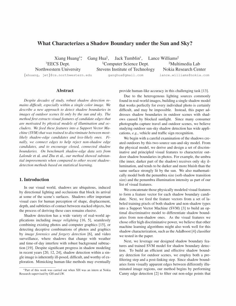
Examining the progressive change of radiance values

along the scan line x perpendicular to the shadow bound-

(a) Shadow cast on a piece of white paper by building roof

(b) Crop a rectangular region that includes the shadow boundary

0 50 100 150 200 2500

1

2

3x 104

position (x)

illum

inat

ion

illumination changes accross the shadow boundary

Red ChannelGreen ChannelBlue Channel

tw

(c) Shadow-to-sunlight illumination changes measured along the scan-line

0 50 100 150 200 250

0.6

0.8

1

1.2

position (x)

illum

inat

ion

red/

blue

illuminaton ratio red/blue changes accross the shadow boundary

(d) Scan-line red/blue ratio: 0.65 in sunlight, 1.1 in shadow

Figure 2. Illumination change across the shadow boundary

ary in Fig. 2(b) reveals important color differences between

sunlight and shadow. We took this photo in raw format with

the T1i camera, and then convert it to a ‘linearized’ 16-bit

TIFF image whose pixel values are linearly proportional to

the scene radiance. We further calibrate the color of the

paper by comparing the average pixel value of a patch of

paper with that of a gray card under the same illumination.

We scale each color channel of the image according to the

paper color to obtain an illumination-only image, and thus

ensure that pixel RGB values in Fig. 2(c) are directly pro-

portional to illumination at each point on the paper.

Careful examination of RGB scanline values plotted

in Fig. 2(c) confirms shadow illumination has a blue

cast, matching the sky’s blue color caused by Rayleigh

scattering[10, 1]. By comparison, the sun-and-sky lit por-

tion shows increased strength in red/yellow components,

greatly increasing the ratio of red/blue at each pixel, plotted

in Fig.2(d). For the mid-range color balance we chose, the

red/blue ratio grows from approximately 0.65 in the shad-

owed region lit only by sky upwards to approximately 1.1

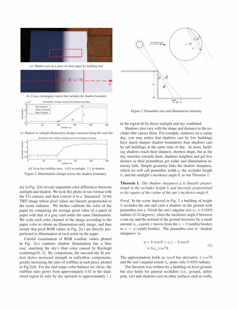
� s�

�

�

Figure 3. Penumbra size and illumination intensity

in the region lit by direct sunlight and sky combined.

Shadows also vary with the shape and distance to the oc-

cluder that causes them. For example, outdoors on a sunny

day, you may notice that shadows cast by low buildings

have much sharper shadow boundaries than shadows cast

by tall buildings at the same time of day. At noon, build-

ing shadows reach their sharpest, shortest shape, but as the

day stretches towards dusk, shadows lengthen and get less

distinct as their penumbrae get wider and illumination in-

tensity falls. Simple geometry links the shadow sharpness,

which we will call penumbra width p, the occluder height

h, and the sunlight’s incidence angle θ, in our Theorem 1:

Theorem 1. The shadow sharpness p is linearly propor-tional to the occluder height h and inversely proportionalto the square of the cosine of the sun’s incidence angle θ.

Proof. In the scene depicted in Fig. 3 a building of height

h occludes the sun and casts a shadow on the ground with

penumbra size p. Given the sun’s angular size φs ≈ 0.0093radians (0.53 degrees), when the incidence angle θ between

a sun ray and the normal of the ground increases by a small

amount φs, a point x moves from the x = 0 (umbra border)

to x = p (sunlit border). The penumbra size or ‘shadow

sharpness’ is:

p = h tan(θ + φs)− h tan θ

≈ hφs/cos2θ.

(1)

The approximation holds as tan θ has derivative 1/cos2θand the sun’s angular extent φs spans only 0.0093 radians.

The theorem was written for a building on level ground,

but also holds for general occluders (i.e., ground, utility

pole, car) and shadows cast on other surfaces such as walls,

by defining h as the distance between the occluder and shad-

owed surface, and θ as the incidence angle between the sun

ray and the surface normal of the shadowed surface.

Together, Theorem 1 and Equation (1) explain why lower

buildings have sharper shadows than tall ones, as shadow

sharpness p is directly proportional to building height h.

We could also infer from Theorem 1 that the shadow

sharpness p is constant for a building with same height,

or vary smoothly along the shadow boundary, because any

physically realizable occluder such as a building must have

a continuous height h. Consequently, the shadow transition

width w (in pixels) in an image is smooth at locally flat sur-

faces in the scene, such as wall and floor. Furthermore, the

average change rate of the pixel values on a scanline cross-

ing this shadow boundary, shown as t/w in the scanline plot

of Fig. 2(c), must be continuous, and must be inversely pro-

portional to shadow sharpness w because t is constant ev-

erywhere in the scene (we assume all shadows receive the

same sky-only illumination).

Later, these two continuous properties simplify the

edge linking process, and will resolve any ambiguities

at T-junctions between shadow boundaries and reflectance

edges, as demonstrated in our experiments in Section 6.

Fig. 2(c) shows a slightly curved and symmetric intensity

profile for the penumbra, with maximal slope at the middle

of the penumbra. Theorem 2 below describes the intensity

change rate in the penumbra.

Theorem 2. Within any image of a scene lit only by thesun and sky, if we choose any straight line perpendicular toa shadow boundary, then the illumination intensity change(or radiance) has a rate proportional to sqrt(1 − (2x/p −1)2) along that line through the penumbra , where x is thedistance to the umbra, and p is the penumbra size.

Proof. As shown in Fig. 3, when the position x along the

scan line (orthogonal to the shadow boundary) changes

from 0 to p, the visible portion of the sun’s surface that

an observer can see from point x will change as well. At

x = 0, we cannot see the sun at all. At x = p, we see

half of the sun’s surface with area 2πr2 for sun radius r. At

0 < x < p within the penumbra, we can see only a portion

of the sun’s surface: a half-spherical cap with height d as

shown in Fig. 3. According to the triangle similarity, we

have d/(2r) = φ/φs = x/p, thus the visible half spherical

cap has area πrd = 2πr2x/p for 0 < x < p.

When we move from x to x+Δx for a small amount Δx,

we will see an increased sun area of 2πr2Δx/p, the surface

area of which has angle (π/2 − α) to the incident sun ray.

The increased visible surface will add an illumination inten-

sity amount that is proportional to (2πr2Δx/p)∗cos(π/2−α). From Fig. 3, we can see cosα = 1 − d/r = 1 − 2x/p,

thus the illumination intensity change rate with respect to x

is proportional to cos(π/2− α) = sqrt(1− (2x/p− 1)2).Note the illumination intensity within the penumbra has its

largest slope at the penumbra’s centerline x = p/2.

Theorem 2 demonstrates that the illumination measured

across the penumbrae for any shadow has the same fixed

shape, which may be another clue to distinguish shadow

boundaries from reflectance boundaries, without regard to

the orientation, shape, or placement of either kind of edge.

Of course, the shape of the shadow boundary may be

smoothed by blur from a poorly focussed camera, and its

intensity profile may get distorted by camera vignetting or

camera sensors with nonlinear responses to radiance, but

underneath these distortions, shadows on flat surfaces will

still exhibit the characteristic features described by Theo-

rem 2.

These physical properties of outdoor shadows motivated

and led us to design a set of discriminative visual features

to characterize shadow boundaries in forms suitable for use

with machine-learning methods.

4. Discriminative Shadow Boundary Features

Very few pixels in an image describe an edge or a bound-

ary of any kind. Our method begins by applying the Canny

edge detection algorithm to identify all the pixels that might

be part of an edge, without regard to the cause of those

edges. In this section we exploit our observations about

shadows from the last section to define several visual fea-

tures. Each one offers indicators about the pixel’s suitability

as a shadow-edge, and we will use sets of these features to

train our chosen machine learning method (SVM) to distin-

guish between edge-candidate pixels that are likely or un-

likely to be part of a shadow edge.

The first visual feature for candidate-edge pixels mea-

sure the illumination ratio of the sun and sky, which dif-

fer substantially across a shadow boundary. We com-

pute the Gaussian weighted average of pixels on both

sides of the edge: the bright, sunlit side has weighted

average Hr, Hg, Hb for red, green and blue channels re-

spectively, and the dark, shadowed side has weighted av-

erage Lr, Lg, Lb. We then compute the intensity ratio

(tr, tg, tb) = (Lr/Hr, Lg/Hg, Lb/Hb). Assuming the re-

flectance is locally uniform near the shadow boundary, the

intensity ratio will match the illumination ratio of the sun

and sky when measured across the shadow boundary. Thus

we can reasonably expect tr > tg > tb at shadow bound-

aries, as the shadow, lit only by the sky, is more bluish than

the sunlit side. Finally, we compute the feature vector as

(t, trb, tgb) = ((tr + tg + tb)/3, tr/tb, tg/tb). This feature

vector encodes the sun and sky illumination difference and

hence offers a more easily-discriminated cue than simply

using (tr, tg, tb) directly.

r�

g�

b�

r�

g�

b� r�

g�b�

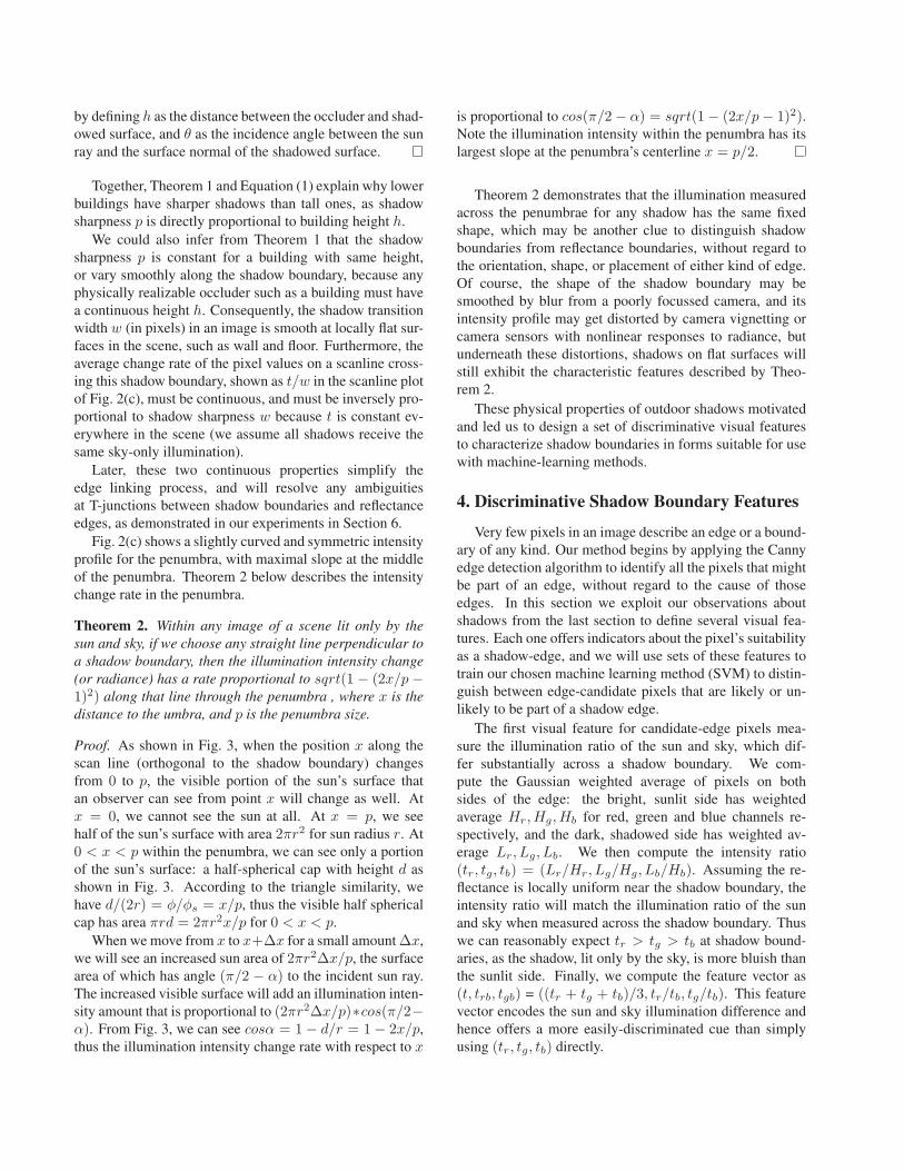
( )a ( )b ( )c

Figure 4. Image gradients computed separately for each RGB color

channel. (a)Shadow edge: same direction. (b)Possible other

edges: opposite but collinear direction (e.g., gradient in green

channel is opposite to gradient in blue channel at the boundary

between pure green material and pure red material). (c)Possible

other edges: more general cases with non-collinear directions.

The second visual feature compares the gradient of il-

lumination of the sun to help identify shadow boundaries.

First, we compute the color gradient magnitude (sr, sg, sb)at each candidate edge pixel. As shown in Fig. 2(c),

(sr, sg, sb) corresponds to the gradient of the sun’s illu-

mination in the penumbra, but includes scaling by the lo-

cal reflectance values. We defined this feature vector as

(δr, δg, δb) = (sr/Hr, sg/Hg, sb/Hb) to cancel the re-

flectance, and to leave behind only the gradient of illumi-

nation.

We construct our third set of features from the color gra-

dient direction (γr, γg, γb). For any candidate edge pixel

at a shadow boundary where reflectance is locally con-

stant, the image gradient should have the same direction in

all color channels, as the RGB illumination gradients are

all perpendicular to the shadow boundary. Other kinds of

edges may lack this property, as demonstrated in Fig. 4.

The third feature vector exploits this distinction by mea-

suring the gradient’s directional difference for each color as

(γrg, γgb, γbr), where γrg = min(|γr−γg|, 2π−|γr−γg|).We found that feeding the SVM with these angular differ-

ences (γrg, γgb, γbr) gave better results than supplying the

original angles (γr, γg, γb) alone, as the the former are ro-

tationally invariant. In our experiment, the variance of gra-

dient direction in different color channels for non-shadow

edges is on average around 15 times larger than that of

shadow edges.

We derive the fourth visual feature vector from the edge

width values in each color channel (wr, wg, wb). As shown

in Fig. 2(c), a shadow boundary should have the same width

for all color channels. We compute this fourth feature vector

as (w,wrg, wrb), where w = (wr + wg + wb)/3, wrg =|wr/wg|, wrb = |wr/wb|. Note Theorem 1 also indicates

that shadow width is a continuous parameter thus we could

also use the edge parameter for shadow edge linking.

In summary, we build a visual feature vector

(t, trb, tgb, δr, δg, δb, γrg, γgb, γbr, w, wrg, wrb) at three

scales at each edge pixel. If we choose an edge pixel actu-

ally located at a shadow boundary, then its 36D (12D times

three scales) visual-feature vector will contain shadow-

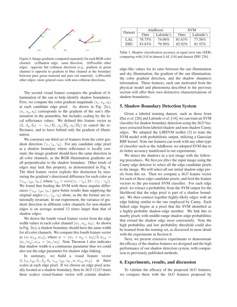
DatasetAdaBoost SVM

Ours Lalonde’s Ours Lalonde’s

LAL 78.75% 74.06% 81.63% 77.56%

ZHU 83.83% 79.50% 85.92% 81.52%

Table 1. Shadow classification accuracy at equal error rate (EER)

comparing with [14] in dataset LAL [14] and dataset ZHU [26].

edge-like values for its ratio between the sun illumination

and sky illumination, the gradient of the sun illumination,

the color gradient direction, and the shadow sharpness

information. These features, each one motivated from the

physical model and phenomena described in the previous

section will offer their own distinctive characterizations of

shadow boundaries.

5. Shadow Boundary Detection SystemGiven a labeled training dataset, such as those from

Zhu et al. [26] and Lalonde et al. [14], we can train an SVM

classifier for shadow boundary detection using the 36D fea-

tures extracted from labeled shadow and non-shadow Canny

edges. We adopted the LIBSVM toolkit [3] to train the

SVM model with probabilistic output, utilizing a Gaussian

RBF kernel. Note our features can work with any other type

of classifier such as the AdaBoost; we adopted SVM due to

its better accuracy manifested in our experiments.

We detect the shadows in a test image with the follow-

ing procedures. We first pre-filter the input image using the

Canny edge detector to select all the edge-candidate pixels

in the image. We will select all our initial shadow-edge pix-

els from this set. Then we compute a 36D feature vector

for each of these edge-candidate pixels, and feed the feature

vectors to the pre-trained SVM classifier. For each edge

pixel, we extract a probability from the SVM output for the

likelihood that the edge pixel is part of a shadow bound-

ary. We then connect together highly-likely edges with an

edge linking similar to the one employed by Canny. Each

linked edge begins at a pixel that the SVM identified as

a highly-probable shadow-edge member. We link this to

nearby pixels with middle-range shadow-edge probabilities

that extend the shadow edge most consistently. Note the

high probability and low probability threshold could also

be learned from the training set, as discussed in more detail

with the experiments in Section 6.

Next, we present extensive experiments to demonstrate

the efficacy of the shadow features we designed and the high

performance of our shadow detection system, with compar-

ison to previously published methods.

6. Experiments, results, and discussionTo validate the efficacy of the proposed 36D features,

we compare them with the 48D features proposed by

0 0.1 0.2 0.3 0.4 0.5 0.6 0.7 0.8 0.9 10

0.1

0.2

0.3

0.4

0.5

0.6

0.7

0.8

0.9

1Comparision of ROC curve and accuracy (EER) for Imag Set Lalonde

False Positive Rate

True

Pos

itive

Rat

e

Ours: SVM: accuracy=81.63%, AUC=0.890Ours: Adaboost: accuracy=78.75%, AUC=0.868Lalonde: SVM: accuracy=77.56%, AUC=0.817Lalonde: Adaboost: accuracy=74.06%, AUC=0.816

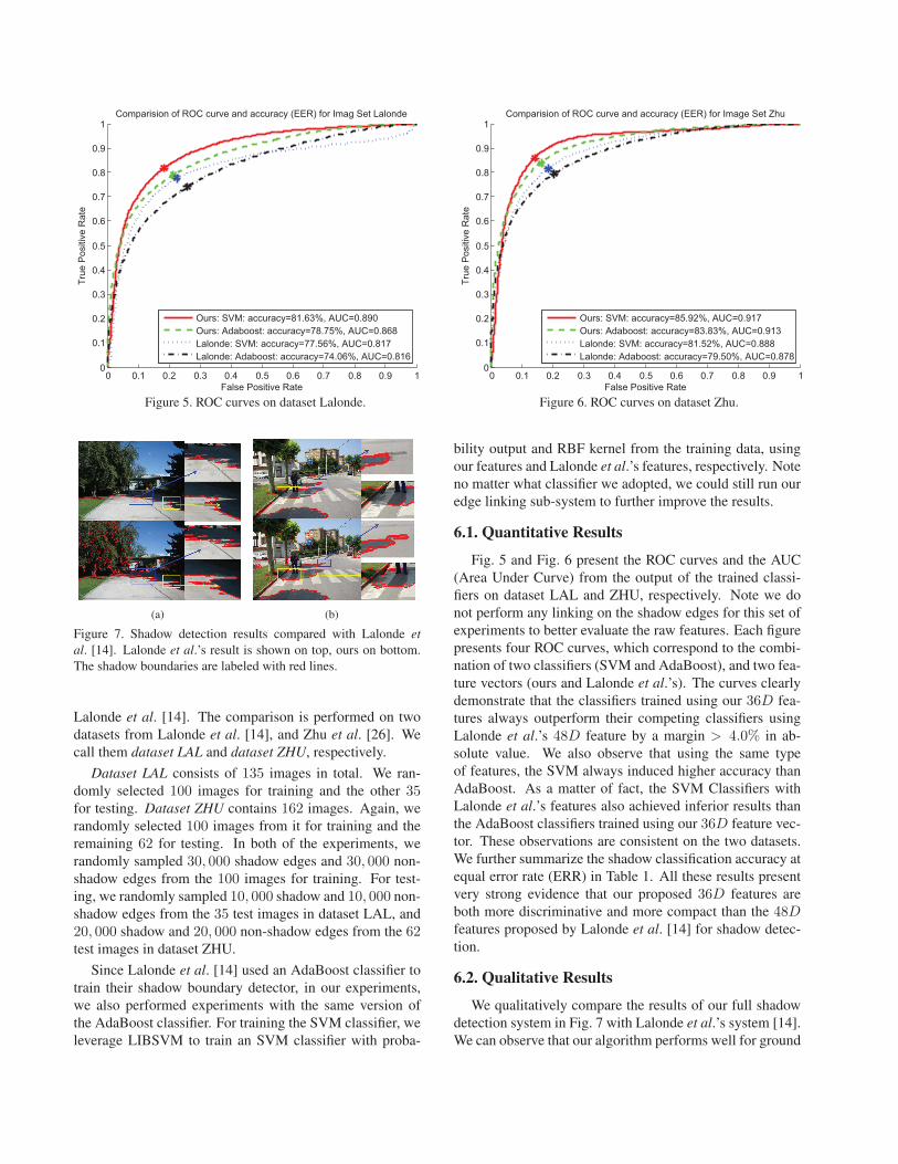
Figure 5. ROC curves on dataset Lalonde.

0 0.1 0.2 0.3 0.4 0.5 0.6 0.7 0.8 0.9 10

0.1

0.2

0.3

0.4

0.5

0.6

0.7

0.8

0.9

1Comparision of ROC curve and accuracy (EER) for Image Set Zhu

False Positive Rate

True

Pos

itive

Rat

e

Ours: SVM: accuracy=85.92%, AUC=0.917Ours: Adaboost: accuracy=83.83%, AUC=0.913Lalonde: SVM: accuracy=81.52%, AUC=0.888Lalonde: Adaboost: accuracy=79.50%, AUC=0.878

Figure 6. ROC curves on dataset Zhu.

(a) (b)

Figure 7. Shadow detection results compared with Lalonde etal. [14]. Lalonde et al.’s result is shown on top, ours on bottom.

The shadow boundaries are labeled with red lines.

Lalonde et al. [14]. The comparison is performed on two

datasets from Lalonde et al. [14], and Zhu et al. [26]. We

call them dataset LAL and dataset ZHU, respectively.

Dataset LAL consists of 135 images in total. We ran-

domly selected 100 images for training and the other 35for testing. Dataset ZHU contains 162 images. Again, we

randomly selected 100 images from it for training and the

remaining 62 for testing. In both of the experiments, we

randomly sampled 30, 000 shadow edges and 30, 000 non-

shadow edges from the 100 images for training. For test-

ing, we randomly sampled 10, 000 shadow and 10, 000 non-

shadow edges from the 35 test images in dataset LAL, and

20, 000 shadow and 20, 000 non-shadow edges from the 62test images in dataset ZHU.

Since Lalonde et al. [14] used an AdaBoost classifier to

train their shadow boundary detector, in our experiments,

we also performed experiments with the same version of

the AdaBoost classifier. For training the SVM classifier, we

leverage LIBSVM to train an SVM classifier with proba-

bility output and RBF kernel from the training data, using

our features and Lalonde et al.’s features, respectively. Note

no matter what classifier we adopted, we could still run our

edge linking sub-system to further improve the results.

6.1. Quantitative Results

Fig. 5 and Fig. 6 present the ROC curves and the AUC

(Area Under Curve) from the output of the trained classi-

fiers on dataset LAL and ZHU, respectively. Note we do

not perform any linking on the shadow edges for this set of

experiments to better evaluate the raw features. Each figure

presents four ROC curves, which correspond to the combi-

nation of two classifiers (SVM and AdaBoost), and two fea-

ture vectors (ours and Lalonde et al.’s). The curves clearly

demonstrate that the classifiers trained using our 36D fea-

tures always outperform their competing classifiers using

Lalonde et al.’s 48D feature by a margin > 4.0% in ab-

solute value. We also observe that using the same type

of features, the SVM always induced higher accuracy than

AdaBoost. As a matter of fact, the SVM Classifiers with

Lalonde et al.’s features also achieved inferior results than

the AdaBoost classifiers trained using our 36D feature vec-

tor. These observations are consistent on the two datasets.

We further summarize the shadow classification accuracy at

equal error rate (ERR) in Table 1. All these results present

very strong evidence that our proposed 36D features are

both more discriminative and more compact than the 48Dfeatures proposed by Lalonde et al. [14] for shadow detec-

tion.

6.2. Qualitative Results

We qualitatively compare the results of our full shadow

detection system in Fig. 7 with Lalonde et al.’s system [14].

We can observe that our algorithm performs well for ground

shadows and yet detects non-ground shadows well when

compared to Lalonde et al. Notice that our shadow detec-

tion is more accurate in terms of localization, especially in

those blue rectangular regions. We can also observe that we

missed fewer shadow boundaries.

We also attack a challenging case pointed out by Zhu etal. [26], where the shadows are cast on water, as shown in

Fig. 8. While Zhu et al.’s features do not capture the prop-

erties of shadows in the water, our feature vector captures

it well, since the shadow is still more bluish than the sun-

lit area. We further show in Fig. 9 our shadow detection

works well for many challenging cases. Our approach suc-

cessfully detects shadows in different contexts, including

foliage shadows on concrete and tarmac, in close-ups and

aerial photos. This shows our features are robust in a wide

variety of outdoor environments.

6.3. Discussions

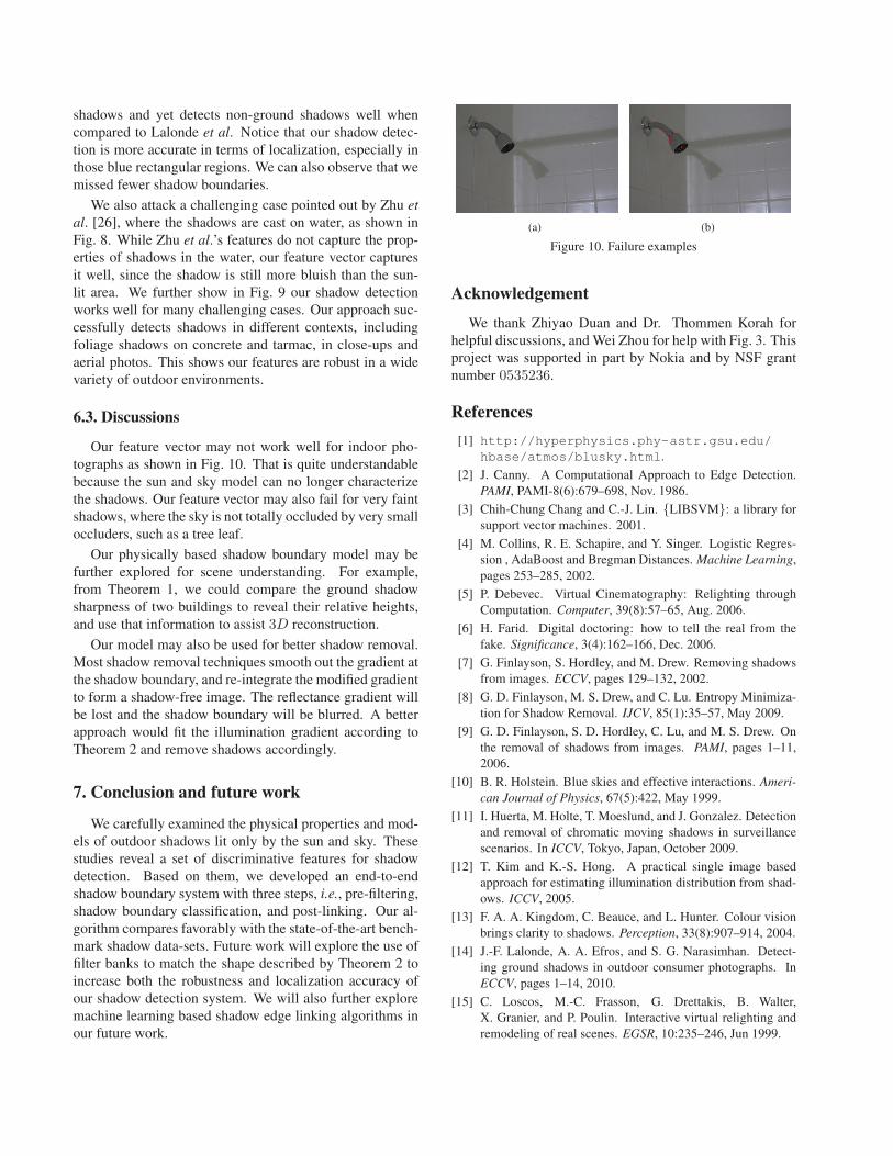
Our feature vector may not work well for indoor pho-

tographs as shown in Fig. 10. That is quite understandable

because the sun and sky model can no longer characterize

the shadows. Our feature vector may also fail for very faint

shadows, where the sky is not totally occluded by very small

occluders, such as a tree leaf.

Our physically based shadow boundary model may be

further explored for scene understanding. For example,

from Theorem 1, we could compare the ground shadow

sharpness of two buildings to reveal their relative heights,

and use that information to assist 3D reconstruction.

Our model may also be used for better shadow removal.

Most shadow removal techniques smooth out the gradient at

the shadow boundary, and re-integrate the modified gradient

to form a shadow-free image. The reflectance gradient will

be lost and the shadow boundary will be blurred. A better

approach would fit the illumination gradient according to

Theorem 2 and remove shadows accordingly.

7. Conclusion and future work

We carefully examined the physical properties and mod-

els of outdoor shadows lit only by the sun and sky. These

studies reveal a set of discriminative features for shadow

detection. Based on them, we developed an end-to-end

shadow boundary system with three steps, i.e., pre-filtering,

shadow boundary classification, and post-linking. Our al-

gorithm compares favorably with the state-of-the-art bench-

mark shadow data-sets. Future work will explore the use of

filter banks to match the shape described by Theorem 2 to

increase both the robustness and localization accuracy of

our shadow detection system. We will also further explore

machine learning based shadow edge linking algorithms in

our future work.

(a) (b)

Figure 10. Failure examples

Acknowledgement

We thank Zhiyao Duan and Dr. Thommen Korah for

helpful discussions, and Wei Zhou for help with Fig. 3. This

project was supported in part by Nokia and by NSF grant

number 0535236.

References[1] http://hyperphysics.phy-astr.gsu.edu/

hbase/atmos/blusky.html.

[2] J. Canny. A Computational Approach to Edge Detection.

PAMI, PAMI-8(6):679–698, Nov. 1986.

[3] Chih-Chung Chang and C.-J. Lin. {LIBSVM}: a library for

support vector machines. 2001.

[4] M. Collins, R. E. Schapire, and Y. Singer. Logistic Regres-

sion , AdaBoost and Bregman Distances. Machine Learning,

pages 253–285, 2002.

[5] P. Debevec. Virtual Cinematography: Relighting through

Computation. Computer, 39(8):57–65, Aug. 2006.

[6] H. Farid. Digital doctoring: how to tell the real from the

fake. Significance, 3(4):162–166, Dec. 2006.

[7] G. Finlayson, S. Hordley, and M. Drew. Removing shadows

from images. ECCV, pages 129–132, 2002.

[8] G. D. Finlayson, M. S. Drew, and C. Lu. Entropy Minimiza-

tion for Shadow Removal. IJCV, 85(1):35–57, May 2009.

[9] G. D. Finlayson, S. D. Hordley, C. Lu, and M. S. Drew. On

the removal of shadows from images. PAMI, pages 1–11,

2006.

[10] B. R. Holstein. Blue skies and effective interactions. Ameri-can Journal of Physics, 67(5):422, May 1999.

[11] I. Huerta, M. Holte, T. Moeslund, and J. Gonzalez. Detection

and removal of chromatic moving shadows in surveillance

scenarios. In ICCV, Tokyo, Japan, October 2009.

[12] T. Kim and K.-S. Hong. A practical single image based

approach for estimating illumination distribution from shad-

ows. ICCV, 2005.

[13] F. A. A. Kingdom, C. Beauce, and L. Hunter. Colour vision

brings clarity to shadows. Perception, 33(8):907–914, 2004.

[14] J.-F. Lalonde, A. A. Efros, and S. G. Narasimhan. Detect-

ing ground shadows in outdoor consumer photographs. In

ECCV, pages 1–14, 2010.

[15] C. Loscos, M.-C. Frasson, G. Drettakis, B. Walter,

X. Granier, and P. Poulin. Interactive virtual relighting and

remodeling of real scenes. EGSR, 10:235–246, Jun 1999.

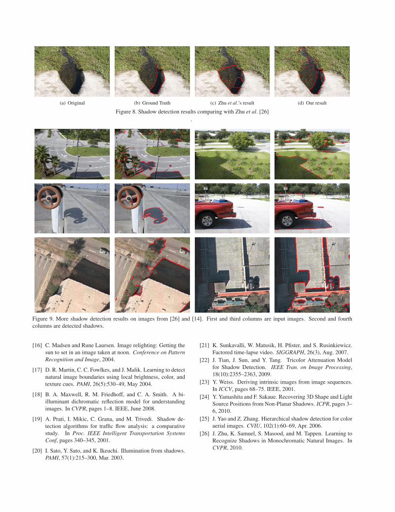
(a) Original (b) Ground Truth (c) Zhu et al.’s result (d) Our result

Figure 8. Shadow detection results comparing with Zhu et al. [26]

.

Figure 9. More shadow detection results on images from [26] and [14]. First and third columns are input images. Second and fourth

columns are detected shadows.

[16] C. Madsen and Rune Laursen. Image relighting: Getting the

sun to set in an image taken at noon. Conference on PatternRecognition and Image, 2004.

[17] D. R. Martin, C. C. Fowlkes, and J. Malik. Learning to detect

natural image boundaries using local brightness, color, and

texture cues. PAMI, 26(5):530–49, May 2004.

[18] B. A. Maxwell, R. M. Friedhoff, and C. A. Smith. A bi-

illuminant dichromatic reflection model for understanding

images. In CVPR, pages 1–8. IEEE, June 2008.

[19] A. Prati, I. Mikic, C. Grana, and M. Trivedi. Shadow de-

tection algorithms for traffic flow analysis: a comparative

study. In Proc. IEEE Intelligent Transportation SystemsConf, pages 340–345, 2001.

[20] I. Sato, Y. Sato, and K. Ikeuchi. Illumination from shadows.

PAMI, 57(1):215–300, Mar. 2003.

[21] K. Sunkavalli, W. Matusik, H. Pfister, and S. Rusinkiewicz.

Factored time-lapse video. SIGGRAPH, 26(3), Aug. 2007.

[22] J. Tian, J. Sun, and Y. Tang. Tricolor Attenuation Model

for Shadow Detection. IEEE Tran. on Image Processing,

18(10):2355–2363, 2009.

[23] Y. Weiss. Deriving intrinsic images from image sequences.

In ICCV, pages 68–75. IEEE, 2001.

[24] Y. Yamashita and F. Sakaue. Recovering 3D Shape and Light

Source Positions from Non-Planar Shadows. ICPR, pages 3–

6, 2010.

[25] J. Yao and Z. Zhang. Hierarchical shadow detection for color

aerial images. CVIU, 102(1):60–69, Apr. 2006.

[26] J. Zhu, K. Samuel, S. Masood, and M. Tappen. Learning to

Recognize Shadows in Monochromatic Natural Images. In

CVPR, 2010.