What Causes Business Cycles?

Analysis of the Japanese Industrial Production Data

Hiroshi Iyetomi, Yasuhiro Nakayama

Department of Physics, Niigata University, Niigata 950-2181, Japan

Hiroshi Yoshikawa

Faculty of Economics, University of Tokyo, Tokyo 113-0033, Japan

Hideaki Aoyama

Department of Physics, Kyoto University, Kyoto 606-8501, Japan

Yoshi Fujiwara

ATR Laboratories, Kyoto 619-0288, Japan

Yuichi Ikeda

Hitachi Ltd, Hitachi Research Laboratory, Ibaraki 319-1221, Japan

Wataru Souma

College of Science and Technology, Nihon University, Chiba 274-8501, Japan

Abstract

We explore what causes business cycles by analyzing the Japanese indus-trial production data. The methods are spectral analysis and factor analysis.Using the random matrix theory, we show that two largest eigenvalues aresignificant. Taking advantage of the information revealed by disaggregateddata, we identify the first dominant factor as the aggregate demand, andthe second factor as inventory adjustment. They cannot be reasonably in-terpreted as technological shocks. We also demonstrate that in terms of twodominant factors, shipments lead production by four months. Furthermore,out-of-sample test demonstrates that the model holds up even under the2008-09 recession. Because a fall of output during 2008-09 was caused by anexogenous drop in exports, it provides another justification for identifying

Preprint submitted to Journal of Japanese and International Economy October 24, 2018

arX

iv:0

912.

0857

v2 [

q-fi

n.G

N]

22

Nov

201

0

the first dominant factor as the aggregate demand. All the findings suggestthat the major cause of business cycles is real demand shocks.

Keywords:JEL No: E23,, E32,

1. Introduction

What causes business cycles? A glance at Haberler (1964) reveals thatall kinds of theories had already been advanced by the end of the 1950’s. Inrecent years, macroeconomists had been so confident of their skillful policymanagement as to hail the “Great Moderation”. Lucas (2003) in his Presi-dential Address to the meeting of the American Economic Association madethe following declaration:

Macroeconomics was born as a distinct field in the 1940’s, as apart of the intellectual response to the Great Depression. Theterm then referred to the body of knowledge and expertise thatwe hoped would prevent the recurrence of that economic disaster.My thesis in this lecture is that macroeconomics in this originalsense has succeeded: Its central problem of depression preventionhas been solved, for all practical purposes, and has in fact beensolved for many decades (Lucas, 2003, p.1).

Ironically, when Lucas delivered this address, the American economy hadbeen on the steady road to the post-war worst recession, perhaps even de-pression. Business cycles are still with us, and await further investigation.

The real business cycle (RBC) theory pioneered by Kydland and Prescott(1982), arguably the most dominant school today, regards changes of totalfactor productivity as the primary cause of business cycles. This theory isbasically the neoclassical equilibrium theory, and minimizes the role of thegovernment’s stabilization policy. The Keynesian theory, in contrast, at-tributes business cycles to fluctuations of real aggregate demand (Summers,1986; Mankiw, 1989; Tobin, 1993), and assigns the government and the cen-tral bank the substantial role of stabilization. The fundamental problem,namely what causes business cycles, remains unresolved.

The standard approach to study this problem is to explore the relative im-portance of technology shocks on one hand and demand shocks on the other

2

as the sources of business cycles by making various identifying restrictions onmacro time-series models: See Shapiro and Watson (1988), Blanchard andQuah (1989), Francis and Ramey (2005) and works cited therein. Thoughvariables used and methods differ in details, they all share the same key iden-tifying restriction. Namely, the level of output (or real GDP) is determinedin the long-run only by supply shocks such as technology shocks. Conversely,the long-run effect of demand shocks on output is assumed to be nil. On thisassumption, not directly observable disturbances are sorted into technologyshocks and demand shocks.1

A majority of works routinely make this assumption without question-ing its validity. However, we maintain that the assumption is not actuallyso tenable as is commonly believed. The problem is that in the study ofbusiness cycles, technology shocks are usually taken exogenous as typified byreal business cycle theory (Kydland and Prescott, 1982). Here, we must ob-serve that modern micro-founded macroeconomics is curiously inconsistentin that while new growth theory puts so much emphasis on the endogeneityof technical progress, business cycle theory is naively content with taking ad-vances in technology as exogenous. New technology or technical progress iscertainly not a free lunch! First of all, it must be generated by R&D invest-ment. Once new technology is found out, it can augment production only byway of investment which embodies such new technology. Now, investmentincluding R&D investment, is, of course, much affected by cyclical fluctua-tions. Monetary factors as well as real factors affect investment. Thus, to theextent that new technology is embodied in investment, demand shocks arebound to affect the pace of technical progress. Therefore, we can not naivelyaccept the standard identifying restriction that demand shocks do not leavethe permanent effects on the level of output.

One way to proceed without this questionable assumption is to take ad-vantage of disaggregated data. The representative works on business cyclescited earlier all use the macro variables. However, business cycles as theconspicuous macro phenomena are characterized by the fact that outputmovements across broadly defined sectors and types of goods move together(Mitchell, 1951). In Mitchell’s terminology, they exhibit high conformity. Itis then most natural to seek possibly unobserved common factors underliningsectoral comovements as the basic factors causing business cycles. Moreover,the separate effects of such unobserved factors on production, shipments andinventory are expected to provide us with valuable information on the causesof business cycles.

3

Factor models precisely fit out purpose (Sargent and Sims (1977), Stockand Watson (1998, 2002)). Stock and Watson (1998, 2002) based on thismethod develop the Diffusion Index to be used for improving forecasting thecyclical fluctuations. In this paper, we take the same approach for a differentpurpose. By examining the relationship between production, shipments, andinventory of twenty-one types of goods, we explore what causes businesscycles. We also show that the model estimated based on the pre-Lehmancrisis (September 15th, 2008) can reasonably explain the post-Lehman (2008-09) recession of the Japanese economy. Our findings are in favor of the oldKeynesian view (Tobin, 1993).

2. Indices of Industrial Production

We use the monthly data of the Indices of Industrial Production (IIP)compiled by the Ministry of Economy, Trade and Industry (METI) of Japan.They are indices of industrial production, producer’s shipments, and pro-ducer’s inventory of finished goods. Details of IIP are in the web site ofMETI, Japan (2008). Here, we simply note that the indices are compiledbased on nearly 500 items (496 for production and shipment indices; 358for inventory). We use the data for the 240 months from January 1988 toDecember 2007. (The data itself is available starting on January 1977, butsome items are missing before January 1988.) We use IIP classified by typesof goods, which is listed in Table 1.

We denote the IIP by Sα,g(tj), where α = 1, 2, and 3 denotes production(value added), shipments, and inventory, respectively. Also, g = 1, 2, . . . , 21denotes 21 categories of goods shown in Table 1, and tj = j∆t with ∆t = 1month, and j = 1, 2, . . . , N for N (= 240) months starting in 1/1988 andending in 12/2007. A typical Sα,1(tj) is shown in Figure 1.

The logarithmic growth-rate rα,g(tj) is defined by the following:

rα,g(tj) := log10

[Sα,g(tj+1)

Sα,g(tj)

], (1)

where j runs from 1 to N − 1 = 239 (:= N ′). The time-series rα,1(tj) isplotted in the bottom panel of Figure 1.

The normalized growth rate wα,g is then defined by

wα,g(tj) :=rα,g(tj)− 〈rα,g〉t

σα,g(2)

4

where 〈·〉t denotes average over time t1, . . . , tN ′ and σα,g is the standard de-viation of rα,g over time. Thus the set {wα,g(t1), wα,g(t2), . . . , wα,g(tN ′)} hasthe average equal to zero, and the standard deviation equal to one. Thenormalization is done because the normalized data are to be used in the sub-sequent analysis of random matrix theory. We also note that the informationrevealed by correlation rather than covariance is sufficient for our study oflead-lag relationships among production, shipments and inventories. In thenext section, we will examine the cyclical behavior of the normalized growthrate (2).

3. The Power Spectrum

There are two basic problems in the study of business cycles. First is toidentify the periodicity. Secondly, we must identify common factors causingsectoral comovements.

In this section, we identify the periodicity. Some economists are skepticalof the stable periodicity of business cycles (Diebold and Rudebusch, 1990). Itis certainly true that when we examine the sample path property of stochasticprocess, we face difficulties in finding or even clearly defining the periodicity.However, it does not necessarily mean that we cannot usefully explore theperiodicity of business cycles. We resort to the standard spectral analysis(see Granger (1966), for example).

The Fourier decomposition is done as follows:

wα,g(tj) =1√N ′

N ′−1∑k=0

wα,g(ωk)e−iωktj , (3)

where the Fourier frequency ωk := 2πk/(N ′∆t), so that ωktj = 2πkj/N ′.Because wα,g(tj) are real-valued, we have2,

w∗α,g(ωk) = wα,g(ωN ′−k). (4)

The normality of wα,g(tj) implies that

wα,g(0) = 0,N ′−1∑k=0

|wα,g(ωk)|2 = N ′. (5)

We define the averaged power spectrum p(ωk) as follows:

p(ωk) =1

M

3∑α=1

21∑g=1

|wα,g(ωk)|2 , (6)

5

where M = 63, the total number of the time series. Recall that we have 21categories of goods each for which there are three different variables, namelyproduction, shipments, and inventory. We note that the following relation issatisfied:

N ′−1∑k=0

p(ωk) = N ′, (7)

due to Eq. (5).Figure 2 shows the behavior of p(ω) of the seasonally-adjusted data3

and the non-adjusted original data as a function of the period T := 2π/ω[months]. Hereafter, we will use units of months for T unless otherwise noted.Since the Fourier components of j = 1, ..., (N ′ − 1)/2 are actually identicalto the components of j = N ′ − 1, ..., (N ′ + 1)/2 because of Eq. (4), we plotonly the former half. Therefore, the lower limit of the data in this plot is2∗N ′/(N ′−1) ≈ 2.008. Also, the non-adjusted data is multiplied by a factor7 in this plot so that the comparison becomes easier.

The original data has high peaks4 at T = 1 year, 6 months, and 3 monthsshowing the presence of significant seasonal fluctuations. We observe thatthey are well-eliminated in the adjusted data.5 We will use the seasonally-adjusted data for the following analysis.

We observe the significant power at low frequencies, T = 60 months (5years) and T = 40 months (3 years and 6 months). One might be temptedto argue that strengths of the cycles T = 120 and T = 239 are comparable tothem. However, for the 239 months our data covers, the T = 120 oscillationoccurs only twice, and the T = 239 only once. Therefore, we disregard themas “one-time” events. Also, one might argue that T = 24 appears to bea possible cycle. But so are many peaks for T < 24. In general, peaks forshorter periods tend to be the results of noise, and one needs to discard them.The criteria for selection of significant periods will be discussed in relationto dominant eigenmodes in Section 5.

We can demonstrate the robustness of the T = 60 and T = 40 cycles.These two cycles have the wavenumber (number of periods in the whole regionof 239 months) k = 4 and k = 6 respectively, so that more accurate valuesof the periods are N ′/k ≈ 59.75 and N ′/k ≈ 39.83. Therefore, if the numberof observations, N ′ is different from the present value, there is actually noFourier-coefficient at these periods. Because of this, one may cast a doubton the robustness of the two cycles. In what follows, we will examine thispoint to demonstrate that the two cycles are quite robust.

6

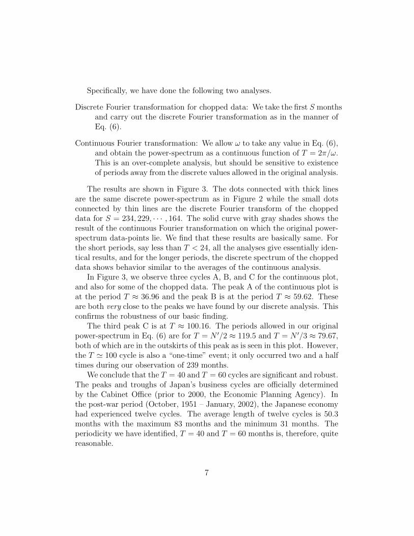
Specifically, we have done the following two analyses.

Discrete Fourier transformation for chopped data: We take the first S monthsand carry out the discrete Fourier transformation as in the manner ofEq. (6).

Continuous Fourier transformation: We allow ω to take any value in Eq. (6),and obtain the power-spectrum as a continuous function of T = 2π/ω.This is an over-complete analysis, but should be sensitive to existenceof periods away from the discrete values allowed in the original analysis.

The results are shown in Figure 3. The dots connected with thick linesare the same discrete power-spectrum as in Figure 2 while the small dotsconnected by thin lines are the discrete Fourier transform of the choppeddata for S = 234, 229, · · · , 164. The solid curve with gray shades shows theresult of the continuous Fourier transformation on which the original power-spectrum data-points lie. We find that these results are basically same. Forthe short periods, say less than T < 24, all the analyses give essentially iden-tical results, and for the longer periods, the discrete spectrum of the choppeddata shows behavior similar to the averages of the continuous analysis.

In Figure 3, we observe three cycles A, B, and C for the continuous plot,and also for some of the chopped data. The peak A of the continuous plot isat the period T ≈ 36.96 and the peak B is at the period T ≈ 59.62. Theseare both very close to the peaks we have found by our discrete analysis. Thisconfirms the robustness of our basic finding.

The third peak C is at T ≈ 100.16. The periods allowed in our originalpower-spectrum in Eq. (6) are for T = N ′/2 ≈ 119.5 and T = N ′/3 ≈ 79.67,both of which are in the outskirts of this peak as is seen in this plot. However,the T ' 100 cycle is also a “one-time” event; it only occurred two and a halftimes during our observation of 239 months.

We conclude that the T = 40 and T = 60 cycles are significant and robust.The peaks and troughs of Japan’s business cycles are officially determinedby the Cabinet Office (prior to 2000, the Economic Planning Agency). Inthe post-war period (October, 1951 – January, 2002), the Japanese economyhad experienced twelve cycles. The average length of twelve cycles is 50.3months with the maximum 83 months and the minimum 31 months. Theperiodicity we have identified, T = 40 and T = 60 months is, therefore, quitereasonable.

7

4. The Dominant Factors Identified by the Random Matrix Theory

Next, we must identify the significant common factors underlying sectoralcomovements. By the common factors, we mean a small number of factorsthat explain the correlation of the original data as much as possible. Weresort to the principal component analysis.

First, we obtain the correlation matrix C as follows;

Cα,g;β,` := 〈wα,gwβ,`〉t (8)

whose diagonal elements are 1 by definition of the normalized growth ratewα,g. Because α and β run from 1 to 3 and g and ` run from 1 to 21, thematrix C has M ×M (M = 63) components.

To uncover the unobservable common factors, we examine the eigenvaluesλ(n) and the corresponding eigenvectors V (n) of the matrix C;

C V (n) = λ(n)V (n). (9)

The eigenvalues λ(n) satisfy the trace-constraint;

M∑n=1

λ(n) = M. (10)

The correlation matrix C is written in terms of the eigenvalues and eigen-vectors as follows:

C =M∑n=1

λ(n)V (n)V (n)T (11)

The distribution of the eigenvalues λ(n) is plotted in Figure 4. We see thatthere are a few isolated large eigenvalues, and that the rest concentrates in thesmaller region. The large eigenvalues and associated eigenvectors correspondto the dominant factors which explain comovements of the fluctuations ofdifferent goods.

The eigenvector corresponding to the largest eigenvalue (which we call“the first eigenvector” hereafter) is the first principal component (PC) thataccounts for as much of the correlation as possible in the M -dimensionalspace. The eigenvector for the second largest eigenvalue (“the second eigen-vector”) is the second principal component that accounts for as much of thecorrelation as possible in the subspace orthogonal to the first eigenvector,and so on.

8

In the principal component analysis (PCA), it remains an unresolvedproblem how to choose significant factors. To solve this problem, manyprocedures and guidelines have been proposed (Jackson, 1991; Jolliffe, 2002;Peres-Neto et al., 2005). For example, the Kaiser-Guttman rule (Guttman,1954; Kaiser, 1960) which is very popular in practice suggests that onlyfactors having eigenvalues greater than one are to be retained. The screegraph named by Cattell (1966) is also widely used. The scree graph is a kindof rank size plot of the eigenvalues of a correlation matrix. In this graph, theabscissa is the rank and the ordinate is the eigenvalue. The typical shape ofthe scree graph is a downward-sloping curve, and the slope changes from the“steep” section to the “shallow” section. Accordingly, we can obtain PCs bylooking for the point that separates the “steep” and the “shallow”. Althoughthe scree graph is used mainly in PCA, Cattell proposes the same methodfor the factor analysis as well.

The problem of testing the significance of a few dominant factors is alsoa challenge to exploratory factor analysis (FA), or the so-called approximatedynamic factor model such as Stock and Watson (1998, 2002). Determin-ing the number of unknown dominant factors has been, in fact, studied inthe rapidly growing literature. Bai and Ng (2002), for example, propose acriteria for the selection of dominant factors in large dimensions of N andT . They basically use the information criteria in a framework of model se-lection. Their analyses are, however, done on the asymptotic assumption oflarge dimensional panels.

Random Matrix Theory

Though how to determine the number of significant components is stillan open issue in PCA and FA, the parallel analysis (PA) proposed by Horn(1965) is considered very likely to be the best procedure (Zwick and Velicer,1986). In PA, the scree graph derived from the actual correlation matrixis compared with that from the random matrix that parallels the originaldata set.6 Because the multivariate time-series of IIP contain uncorrelatedshocks and “measurement” errors, the empirical correlation matrix is to someextent random. It is, therefore, reasonable to compare the properties of theempirical correlation matrix C to a null hypothesis on purely random matrixwhich one would obtain with time-series of totally uncorrelated fluctuations.This is the basic idea of the PA.

We apply the method of random matrix theory (RMT) to the problem ofcomparing the properties of the empirical correlation matrix C with the null

9

hypothesis based on the purely random matrix. The RMT has made greatsuccess in physical sciences, and has quickly found applications to variousdisciplines. We note that the RMT has been applied to finance for a decade(see the textbook by Bouchaud and Potters (2000) and references therein)and macroeconomics (Ormerod, 2008).

PA is widely applied to various disciplines, but it requires the Monte-Carlosimulation to obtain the scree graph for the random matrix. The drawbackof the Monte-Carlo simulation is cost of computation time. Several methodshave been proposed to overcome this problem. For example, the tables ofsimulated eigenvalues of the random matrix with different sample size andnumber of variables are provided by Buja and Eyuboglu (1992). However,if we can obtain the theoretical formula for the probability density function(PDF) for the eigenvalue of the random matrix with different sample sizeand number of variables, we can overcome this drawback of the Monte-Carlosimulation and PA. That is what we will do in what follows.

Let us consider an ensemble of random matrices in which all the elementsof a square matrix A of size M ×M are iid (independent and identically-distributed) random variables with the constraint that Aij = Aji. As aconsequence of the central limit theorem, in the limit of large matrices, thedistribution of eigenvalues has universal properties, which are mostly inde-pendent of the distribution of the elements Aij. In particular, it can beshown that if the Aij’s are iid random variables of zero mean and variance〈A2

ij〉 = σ2/M , the probability density function (PDF) of eigenvalues of A isgiven by the so-called “semi-circle law” (Wigner, 1955):

ρ(λA) =1

2πσ2

√4σ2 − λ2A, (12)

for |λA| ≤ 2σ and zero elsewhere (see Bouchaud and Potters (2000)).Its relevance to our study of correlation is obvious when sample correla-

tion matrix is written as C = ATA where A is a rectangular matrix of sizeM × N (M and N respectively the number and length of time-series), andAT is the transpose of A. If M = N , the eigenvalue λ of C can be obtainedfrom the obvious relation λ = λ2A. If it is assumed that the elements of A areiid random variables, the PDF of eigenvalues of C can be easily calculatedfrom the semi-circle law (12) by using the relation ρ(λ)dλ = 2ρ(λA)dλA (forλA > 0) as

ρ(λ) =1

2πσ2

√4σ2 − λ

λ, (13)

10

for 0 ≤ λ ≤ 4σ2 and zero elsewhere.IfM 6= N , one can derive a similar PDF (Marcenko and Pastur (1967); see

Bouchaud and Potters (2000) for a simple derivation). Using our notations inthis paper of M and N ′, the PDF for the eigenvalue of the M×M correlationmatrix C for M stochastic variable of length N ′ with standard deviation σis given by

ρ(λ) =

Q

2πσ2

√(λ+ − λ)(λ− λ−)

λfor λ− < λ < λ+,

0 otherwise,

(14)

in the limit ofM →∞, N ′ →∞ (15)

with Q := N ′/M fixed. The bounds λ± for λ are defined as follows:

λ± := σ2 (1±√Q)2

Q. (16)

Note that (14) is reduced to (13) when M = N ′.Though the above results (Eqs.(14)–(16)) hold exactly true only asymp-

totically in the limit (15), we emphasize that the RMT is actually robustwith respect to sample size; it holds up not only asymptotically but also forfinite sample with nontrivial autocorrelation. We demonstrate it in AppendixA with the help of a Monte-Carlo analysis of randomized data. Given thisresult, in what follows, we perform significance test of eigenvalues based onthe RMT advanced in physics.

The dashed line in Figure 4 shows the prediction of RMT, Eq. (14) and(16), where in the present case,

σ = 1, Q =239

63≈ 3.79, λ+ ≈ 2.29, λ− ≈ 0.24. (17)

We find that two largest eigenvalues

λ(1) ≈ 9.95, λ(2) ≈ 3.82, (18)

are significant in comparison with the RMT prediction. That is, they are sig-nificantly above the upper bound λ+ and, therefore, reflect the non-randomstructure of the data.

11

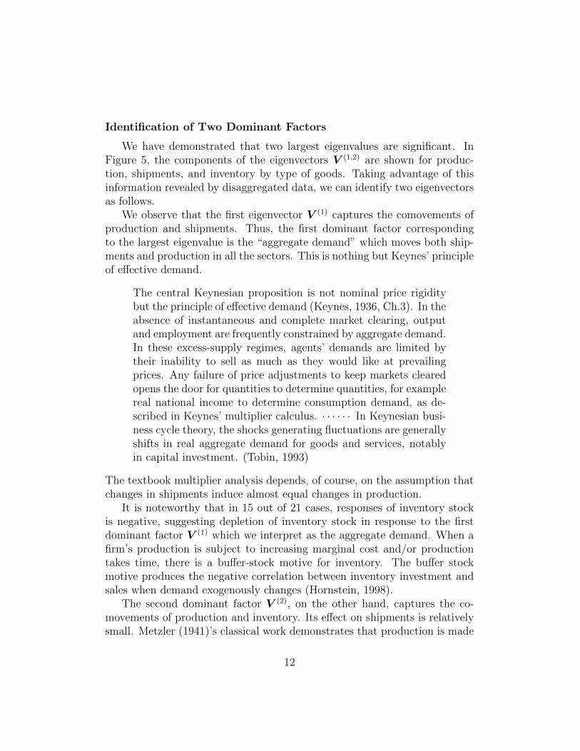
Identification of Two Dominant Factors

We have demonstrated that two largest eigenvalues are significant. InFigure 5, the components of the eigenvectors V (1,2) are shown for produc-tion, shipments, and inventory by type of goods. Taking advantage of thisinformation revealed by disaggregated data, we can identify two eigenvectorsas follows.

We observe that the first eigenvector V (1) captures the comovements ofproduction and shipments. Thus, the first dominant factor correspondingto the largest eigenvalue is the “aggregate demand” which moves both ship-ments and production in all the sectors. This is nothing but Keynes’ principleof effective demand.

The central Keynesian proposition is not nominal price rigiditybut the principle of effective demand (Keynes, 1936, Ch.3). In theabsence of instantaneous and complete market clearing, outputand employment are frequently constrained by aggregate demand.In these excess-supply regimes, agents’ demands are limited bytheir inability to sell as much as they would like at prevailingprices. Any failure of price adjustments to keep markets clearedopens the door for quantities to determine quantities, for examplereal national income to determine consumption demand, as de-scribed in Keynes’ multiplier calculus. · · · · · · In Keynesian busi-ness cycle theory, the shocks generating fluctuations are generallyshifts in real aggregate demand for goods and services, notablyin capital investment. (Tobin, 1993)

The textbook multiplier analysis depends, of course, on the assumption thatchanges in shipments induce almost equal changes in production.

It is noteworthy that in 15 out of 21 cases, responses of inventory stockis negative, suggesting depletion of inventory stock in response to the firstdominant factor V (1) which we interpret as the aggregate demand. When afirm’s production is subject to increasing marginal cost and/or productiontakes time, there is a buffer-stock motive for inventory. The buffer stockmotive produces the negative correlation between inventory investment andsales when demand exogenously changes (Hornstein, 1998).

The second dominant factor V (2), on the other hand, captures the co-movements of production and inventory. Its effect on shipments is relativelysmall. Metzler (1941)’s classical work demonstrates that production is made

12

not only for the purpose of meeting the current sales or shipments but alsofor maintaining the firm’s desired level of inventory stocks. The firm’s desiredlevel of inventory stocks depends on anticipations of future demand or sales.That is, inventory investment becomes, in part, “speculative”. In fact, basedon a robust stylized fact that the variance of production is greater than thatof shipments, Blinder and Maccini (1991) and others have demonstrated thatthe role of inventory stock is not confined to production smoothing. Rather,they show that inventories apparently destabilize output at the macro level.Whether originated from the Metzlerian inventory accelerator (the idea thatdesired inventory stocks rise with sales) or from the (S, s) inventory strategyat the micro level, inventory and production tend to move together. Our sec-ond dominant factor V (2) appears to capture this channel. For convenience,we call it “inventory adjustments”.

Whether direct or indirect, V (1) and V (2) are basically demand factors. Itis difficult to interpret V (1) and V (2) as “productivity shocks” for the follow-ing reason. Changes in total factor productivity (TFP) emphasized by RealBusiness Cycle theory such as Kydland and Prescott (1982) bring changes inmarginal cost in production. In order to minimize costs, the firm increases(decreases) production and accumulates (reduces) inventories during timeswhen marginal cost is low (high). Thus, not only final demand (consumption/ investment) usually analyzed by RBC but inventory investment also movestogether with production when productivity changes (Hornstein, 1998). Inother words, productivity shocks, temporary shocks in particular, must moveall the variables, namely production, shipments, and inventory in tandem.Figure 5 clearly shows that V (1) captures the comovements of production andshipments while V (2) the comovements of production and inventory, leavingthe third variable relatively unaffected in both cases. The two dominantfactors, therefore, do not represent productivity shocks.

5. Dominant Eigenmodes and the Business Cycles

So far, we have found that (1) the T = 60 (months) and the T = 40fluctuations are significant, and also that (2) two largest eigenvalues, λ(1,2)

of the correlation matrix, are significant based on the RMT.These two findings suggest that the contribution of two largest eigen-

value components at T = 60 and T = 40 periods are properly defined as the“business cycles”. In this section, we measure the contribution of this “busi-ness cycle” factor in economic fluctuations. Toward this goal, we express the

13

normalized growth rate in Fourier modes of the eigenvectors.First, we decompose the normalized growth rate wα,g(tj) on the basis of

the eigenvectors V (n);

wα,g(tj) =M∑n=1

an(tj)V(n)α,g . (19)

By substituting this into Eq. (8) and comparing it with Eq. (11), we findthat

〈anan′〉t = δnn′λ(n). (20)

The Fourier decomposition of the coefficients an(tj) is

an(tj) =1√N ′

N ′−1∑k=0

an(ωk) e−iωktj , (21)

similar to Eq. (3). This leads to

λ(n) =1

N ′

N ′−1∑k=0

λ(n)(ωk), λ(n)(ωk) := |an(ωk)|2 . (22)

From Eq. (3) and Eq. (22), we obtain

wα,g(ωk) =M∑n=1

an(ωk)V(n)α,g . (23)

Substituting this into Eq. (6), we obtain that the following decomposition ofthe power spectrum

p(ωk) =1

M

M∑n=1

λ(n)(ωk). (24)

By summing the both-hand sides over k, we recover Eq. (10):

1 =1

N ′

N ′−1∑k=1

p(ωk) =1

M

M∑n=1

λ(n). (25)

This shows that the eigenvectors corresponding to the larger eigenvalues havelarger contribution to the power spectrum on average: For example, the

14

relative contribution of the first eigenvector is 16% as λ(1)/M ≈ 0.16 (M =63). If the contributions of all the eigenvectors were the same, it would beonly 1.6% (1/M ≈ 0.016). The sum of the relative contribution of the firstand the second eigenvector components amounts to 21%. Dominance of twolarge eigenvalues is clear.

So far, we have discussed the average contribution. The important ques-tion is in what part of the power spectrum the large eigenvalues have sig-nificant contributions. Figures 6 and 7 answer this question. In Figure 6,the dark gray spectrum at the bottom is the contribution of the first eigen-vector, λ(1)(ωk)/M , whereas the spectrum with lighter shading is that of thesecond eigenvector, λ(2)(ωk)/M . The solid black line is the whole spectrum,p(ωk), which is the same as the spectrum with gray shading in Figure 2. Weobserve that the eigenmodes of the larger eigenvalues tends to have greatercontributions as T gets larger.

This is better illustrated in Figure 7 which shows the relative contributionin each bin of period with the same notations as used in Figure 6. We observehere that the relative contribution of the first eigenmode is about 20% forT & 40 whereas it is only 10% or less for T . 40. The same is true forthe second eigenmode. The sum of the relative contribution of the first andsecond eigenmodes is about 40% for T & 38 but is only 20% for T . 38.(The boundary T ≈ 38 is denoted by the vertical dashed line and the mark“A” on the horizontal axis.) This is another reason why we rejected smallerperiods like T = 24 as insignificant in Section 3; The relative contributionsof the dominant two eigenmodes for T . 38 are much smaller than those forT = 40 and T = 60. It suggests that fluctuations in shorter periods T < 38are basically due to noises, and do not reflect of any systematic comovements.

We have identified the two dominant factors V (1) and V (2) as demandfactors, not productivity shocks. It is important to recognize that the factthat the relative contribution of V (1) and V (2) is roughly 40% does not meanthat the residual 60% is to be explained by other systematic factors such as“productivity shocks” emphasized by RBC. The residual 60% is to be ex-plained by V (j) (j = 3, 4, . . .), but the significance of V (j) (j = 3, 4, . . .) isrejected by the RMT (Section 4). The residual 60% is, therefore, not reallya part of systematic “business cycles”, but rather caused by various uniden-tified random factors. In fact, Slutzky (1937) suggested that the summationof pure random shocks might generate apparently “cyclical” fluctuations; Ineffect, he rejected the existence of systematic “business cycles”. Contrary tohis assertion, our findings confirm the presence of business “cycles” which

15

systematically account for 40% of economic fluctuations. Such “business cy-cles” defined based on V (1) and V (2) at T = 40 and 60 are basically caused bydemand factors. In the next section, we will investigate the cyclical behaviorof production, shipments and inventory in greater detail.

6. Production and Shipments

In the previous sections, we have shown the presence of the two eigen-modes of the correlation matrix for the T = 40 and 60 Fourier modes. Letus now recover the behavior of production and shipments in these dominantmodes. In order to do so, we first express the decomposition of the IIP datato each Fourier and eigenmode by combining Eqs. (19) and (21):

wα,g(tj) =1√N ′

M∑n=1

N ′−1∑k=0

an(ωk) e−iωktjV (n)

α,g (26)

=2√N ′

M∑n=1

(N ′−1)/2∑k=1

<(an(ωk)e

−iωktj)V (n)α,g . (27)

Here we used the facts that an(0) = 0 due to wα,g(0) = 0, an(ωk) = a∗n(ωN ′−k)due to an(tj) being real, and that N ′ − 1 = 238 is even. The “businesscycle component” is obtained by limiting the above sum to over only k = 4(T = 60) and k = 6 (T = 40) and n = 1, 2.

Figure 8 shows the cyclical movements of production, shipments, andinventory. As explained in the previous section, they are defined as cyclesproduced by two dominant factors at T = 40 and T = 60. The cycles shownin Figure 8 are the average values over the goods, wα(tj) :=

∑21g=1wα,g(tj)/21

for T = 60 (the left panel) and for T = 40 (the right panel). The top rowin each panel is for the first dominant factor, the middle row for the seconddominant factor, and the bottom row for their sum.

In the first eigenmode (the top row), production (the solid line) andshipments (the dashed line) move together with equal amplitude. In contrast,in the second eigenmode (middle) the movements of shipments are almostflat. This is consistent with the results in Figure 5.

Recall that we identify the first eigenmode with the aggregate demandwhile the second eigenmode with inventory adjustments. It is notable thatalthough in each eigenmode, production and shipments move with the same(or opposite) phase as is guaranteed by our expansion, they are shifted in

16

time once the sum over two dominant eigenmodes is done. This is becauseof the difference in their amplitudes.

For the T = 60 oscillations, production is delayed by the second eigen-mode as shown by two black arrows in Figure 8. In contrast, shipmentsreceive almost no contribution from the second eigenvector. As a result, pro-duction is delayed a little after shipments. We can exactly derive this delay-time. From decomposition (26), we see that the average of the normalizedgrowth rates wα,g over the goods (g = 1, . . . 21), wα(tj) :=

∑21g=1wα,g(tj)/21,

contains the following T = 60 (k = 4) part:

wα(tj) =1√N ′

[a1(ω4)V

(1)α + a2(ω4)V

(2)α

]e−iω4tj + · · · . (28)

where V(n)α :=

∑21g=1 V

(n)α,g /21. Therefore, denoting the absolute value and the

phase of the coefficients as,

a1(ω4)V(1)α + a2(ω4)V

(2)α := Aαe

iφα , (29)

where Aα > 0, we find that production (α = 1) and shipment (α = 2) obeythe following relations:

w1(tj) = A1e−i(ω4tj−φ1) + · · · , (30)

w2(tj) = A2e−i(ω4tj−φ2) + · · · . (31)

This means that the delay-time of production behind shipments for the periodT = 60, ∆

(SP)60 , is given by (φ1 − φ2)/ω4. Because ωj = 2πj/N ′ [1/month]

with N ′ = 239, we obtain the delay-time ∆(SP)60 in units of months as follows:

∆(SP)60 :=

239

4

1

2πArg

[a1(ω4)V

(1)1 + a2(ω4)V

(2)1

a1(ω4)V(1)2 + a2(ω4)V

(2)2

]≈ 4.28. (32)

It is clear in this expression that the lead-lag between shipments andproduction is caused by the combination of two eigenmodes. For inventory,the shift occurs in the opposite direction, and as a result, it lags by

∆(PI)60 ≈ 10.95, (33)

behind production.

17

The basically same story holds for the T = 40 oscillations (Figure 8). Wethus obtain7

∆(SP)40 ≈ 1.93, ∆

(PI)40 ≈ 13.62. (34)

We can formally test whether the time-delays ∆(SP)60 and ∆

(SP)40 are sta-

tistically significant or not. Toward this goal, we randomize the rest of theeigenmodes and evaluate those values. The simulation is done in followingsteps:

1. Subtract the eigenmodes of the first two eigenvalues from the actualdata to define:

w′α,g(tj) := wα,g(tj)−2∑

n=1

an(tj)V(n)α,g . (35)

(see Eq. (19)).

2. Randomly reorder the time-series w′α,g(tj) separately, i.e., with ran-domization different for each α and g.

3. Combine the reshuffled part with the first two eigenmodes to create asimulated data.

4. Calculate the eigenvalue distribution and see whether the largest twoeigenvalues still remain. If they are, we proceed to the next step. (Notethat the above randomization process changes the eigenvalues.)

5. Calculate ∆(SP)60 and ∆

(SP)40 for the resulting simulated data.

In this manner, the noise part (the eigenmodes except for the first and secondeigenmodes) are reshuffled. We then check whether the values we obtain

for the time-delays, ∆(SP)60,40 and ∆

(PI)60,40, stand out against the noises. We

carried out this simulation 105 times. The result obtained is that the firsttwo eigenvalues always exist as seen in Figure 9. The distribution of thetime-delays are shown in Figure 10 with the summary statistics of simulationresults in Table 2. We observe that the delay-time obtained in Eqs. (32) and(34) are statistically significant.

In Appendix B, we perform cross-spectrum analysis and estimate thephase in the spectrum to obtain the lead-lag relationships among produc-tion, shipments and inventory. For the series of the sum of the first andsecond eigenmodes, the results obtained by the cross-spectrum analysis areconsistent with, and thereby confirm from a different angle, those presentedin this section. In addition, by comparing them with the cross-spectrum for

18

the original data, we can say that the extraction of the two dominant eigen-modes or our definition of “business cycles” is essential for understanding thelead-lag relationship between shipments and production.

The sum of the components of the first and the second eigenvectors atthe T = 40 and T = 60 periods is compared with the original data forproduction, shipments and inventory in Figure 11. To make comparisoneasier, we applied a simple moving average operation to the original dataover one-year period. For the original data so smoothed out, we can hardlydetect any lead-lag relation between production and shipments. In contrast,in the extracted “business cycles”, shipments clearly precede production withthe average lead time of four months.

In Figure 11, we observe a close one-to-one correspondence between theoriginal data and the extracted business cycles. The peaks and troughs oftwo cycles coincide very well although their amplitudes slightly differ duepossibly to economic fluctuations with longer cycles (T > 60) and exter-nal shocks. A linear combination of two sinusoidal functions oscillating atdifferent periods gives rise to an extended cyclic motion with the period ofT = 120. Figure 11 thus spans two cycles of the endogenous business fluctu-ations. The characteristic behavior of the original data shown in the bottompanel is well captured by the “business cycles” defined here.

Japan had experienced a long stagnation beginning 1990 through 2002.One might consider a possible “structural break” during the “lost decade”.However, the finding of such steady cycles shown in Figure 11 suggests thatthe Japanese economy has had actually a fairly stable structure over the lasttwo decades. Besides, our sample period (January, 1988–December, 2007)basically covers the whole period of the long stagnation. Thus, rather thanchopping our data into sub-sample periods, we resort to the out-of-sampleexamination of the 2008-09 economic crisis in the next section.

We have found that production lags behind shipments over the extracted“business cycles”. It does so inventory adjustments tend to lag behind theinitial changes in shipments. Suppose that shipments or final demand in-creased in the economy as a whole. It induces a contemporaneous increaseof production, and at the same time, depletion of inventory stock in manysectors and also for many types of goods; This is well captured by the firsteigenmode which we interpret the “aggregate demand” (the top panel of Fig-ure 8). Now, an increase of final demand and depletion of inventory stockmake firms revise their expectations on future demand, and accordingly thelevel of desired inventory stock. If demand does not increase further, firms

19

produce more for the purpose of inventory accumulation. This is captured bythe second eigenmode which we interpret the “inventory adjustments” (themiddle row of Figure 8). As Metzler (1941) shows, inventory adjustmentstake time. This makes production lag behind shipments. Our analysis showsthat the average lag is about 4 months. In the case of inventory stock, anincrease of shipments initially causes depletion of inventory, and, therefore,the lag becomes even longer than in the case of production. We find thatthe average lag of inventory behind shipments is about 11 months. In thisway, we can easily understand that shipments lead production and inventorywithin the framework in which changes in real demand or shipments are themajor shocks. Note that productivity shocks emphasized by RBC, by defi-nition, instantaneously change production. There is no room for productionto lag behind shipments in such framework.

7. The 2008-09 Economic Crisis

The 2008-09 financial crisis triggered by the bursting of the housing bub-bles in the U.S. immediately spread all over the world, and caused greatdamage on the global economy, reminiscent of the Great Depression. Basedon the analyses in the previous sections, we update the IIP data to coverthe period from January 2008 (j = 241) through June 2009 (j = 258), andperform an out-of-sample test.

The extended data shown in Figure 12 demonstrates a dramatic drop ofproduction in Japan. Panel (a) of Figure 13 shows the volatility P (t) of theIIP defined by

P (t) :=3∑

α=1

21∑g=1

|wα,g(t)|2. (36)

We observe the exceptionally large amplification of P (t) during the 2008-09economic crisis.

This situation, therefore, provides us with a perfect opportunity for out-of-sample test for validity of the dominant eigenmodes that we have identifiedusing the random matrix theory. To this end, we decompose the extendedIIP data based on the exactly same eigenvectors as in Eq. (19). Then P (t)is expressed in terms of the mode amplitude coefficients an(t) as follows:

P (t) =63∑n=1

|an(t)|2. (37)

20

Panels (b) and (c) of Figure 13 show the partial contributions of the largestand the second largest modes to P (t), respectively. Plainly, an unprecedentedrise of volatility of the first dominant factor, namely |a1(t)|2 accounts largelyfor a rise of P (t) during the 2008-09 crisis. The contribution of the seconddominant factor is not so great as that of the first dominant factor.

The relative contributions of the first and second eigenmodes defined by

πn(t) :=|an(t)|2

P (t). (38)

are shown in Figure 14. The total sum of πn(t) with respect to n is normalizedto unity. The first dominant eigenmode accounts for almost a half of the totalpower of fluctuations during the 2008-09 recession. Note that the relativecontribution of the first eigenmode, namely about one half, is comparable tothat for the in-sample period. This result demonstrates that our factor modelholds up over the 2008-09 crisis despite of the fact that a fall of industrialproduction during the period as shown in Figure 12 was truly unprecedented.

We have seen that the first eigenmode basically explains a fall of indus-trial production during 2008-09. Now, Figure 15 shows IIP and the indexof exports during the period under investigation. Plainly, production fell inresponse to a sudden decline in exports. We emphasize that a fall of exportswas caused by a sudden shrinkage of the world trade due to the financialcrisis accompanied by the global recession, and that it was basically exoge-nous to the Japanese economy . In Section 4, by analyzing the componentsof eigenvectors (Figure 5), we identified the first dominant factor as the ag-gregate demand. To the extent that we identify a sudden fall of exports, anexogenous negative aggregate demand shock, as the basic cause of the 2008-09 recession, the dominance of the first eigenmode provides us with anotherjustification for our interpreting it as the aggregate demand factor. Thisconfirms once again the validity of the Old Keynesian View (Tobin, 1993).

8. Concluding Remarks

In his comments on Shapiro and Watson (1988) entitled “Sources of Busi-ness Cycle Fluctuations,” Hall (1988) made the following remark:

All told, I find the results of this paper harmonious with theemerging middle ground of macroeconomic thinking. There are

21

major unobserved determinants of output and employment oper-ating at business-cycle and lower frequencies. Some are techno-logical, some are financial, some are monetary (Hall, 1988, p.151).

For finding out such unobserved determinants of business cycles, the stan-dard identifying restriction is that only technology shocks affect output per-manently. As discussed in Introduction, we maintain that this assumptionis untenable. Using production, shipments, and inventory data, we analyzethe causes of business cycles more straightforwardly than in the standardapproach.

We have identified (i) two periods T = 60 and 40 months for the Japanesebusiness cycles, and also (ii) the two significant factors causing comovementsof IIP across 21 goods. Taking advantage of the information revealed by dis-aggregated data, we can reasonably interpret the first factor as the aggregatedemand, and the second factor as intentional inventory adjustments. It is dif-ficult to interpret the two dominant factors as productivity shocks. Withinthe framework of the standard RBC, productivity shocks are expected toaffect production, shipments, and inventory together. The two dominantfactors we have identified do not fulfill this condition (Figure 5).

We have also found that, for the part of shipments and production ex-plained by two factors, shipments lead production by a few months. Thislead-lag relationship between shipments and production caused by inventoryadjustment is not clearly seen in the original data. However, inventory ad-justments which generate this lead-lag relationship between shipments andproduction are an important part of “business cycles” defined by two domi-nant factors.

Furthermore, out-of-sample analysis of the 2008–09 recession demon-strates that the first dominant factor largely explains this major episode. Weknow that it was basically caused by a sudden fall of exports beginning thefourth quarter of the year 2008 (Figure 15). Therefore, to the extent that ex-ports can be reasonably regarded as exogenous real aggregate demand shocksto the Japanese economy, we can identify the first dominant factor as thereal aggregate demand. All these findings suggest that the major cause ofbusiness cycles is real demand shocks accompanied by significant inventoryadjustments.

It is important to recognize that this conclusion of ours does not necessar-ily mean that technology shocks are unimportant. On the contrary, it is veryplausible that a major driving force of fixed investment is technology shocks.

22

Furthermore, one might argue that technology shocks is also a driving forceof consumption by way of introduction of new products (Aoki and Yoshikawa,2002). The point is that technology shocks affect the macroeconomy by wayof changes in aggregate demand, notably investment, in the short-run. Forthe purpose of studying business cycles, it is wrong to consider technologyshocks as direct shifts of production function.

The conclusion we drew from our analyses of the Japanese industrialproduction data is clear. To study whether the same results hold up forother economies is obviously an important research agenda. We believe thatthe methods we employed in the present paper can be usefully applied to thestudy of business cycles in other economies.

Finally, we have identified 40 to 60 months “cycles” of aggregate demand.The theory of such “cycles” of aggregate demand is beyond the scope ofthe present paper. After all, the multiplier-accelerator model of Samuelson(1939) and Hicks (1950) may be an answer. The problem awaits furtherinvestigation.

Acknowledgments

We gratefully acknowledge detailed comments made by two anonymousreferees and the editor’s kind suggestions. This work was supported in partby the Program for Promoting Methodological Innovation in Humanities andSocial Sciences by Cross-Disciplinary Fusing of the Japan Society for thePromotion of Science.

23

Appendix A. Significance of Dominant Factors in Finite Sample

We have found that two large eigenvalues exist outside the range of theRMT prediction for the covariance matrix C of IIP. This result, however,holds exactly true only asymptotically in the limit (15), while we have onlyfinite sample, N ′ = 239 and M = 63. Also the RMT applies theoreticallyto iid data as noted in Section 4. In this appendix, we will first show thatnontrivial autocorrelation exists for the growth rate, and then present a sim-ulation result which shows that in spite of the “finite-size” effect and thenontrivial autocorrelation, the dominant factors we have found are still sig-nificant.

The autocorrelation R(t) of the normalized growth rate wα,g is definedby the following:

Rα,g(tm) :=1

N ′ −m

N ′−m∑j=1

wα,g(tj)wα,g(tj+m). (A.1)

By definition, Rα,g(0) = 1, and if there are no autocorrelations, Rα,g(tm) = 0for m ≥ 1. Figure 16 shows the autocorrelation averaged over the goods;

Rα(tm) :=1

21

21∑g=1

Rα,g(tm). (A.2)

We observe that for both production (α = 1) and shipments (α = 2), theautocorrelations have nontrivial values for t = 1 month: R1(1) ≈ −0.31 andR2(1) ≈ −0.39, while we have R3(1) ≈ 0.007 for inventory.

Since this nontrivial autocorrelation, in addition to the finiteness of thedata size, may bring corrections to the RMT results, we have done a simu-lation in the following steps:

(1) Random “rotation” of each time-series,

wα,g(tj)→ wα,g(tMod(j−τ,N ′)) (A.3)

where τ ∈ [0, N ′− 1] is a (pseudo-)random integer, different for each αand g.

(2) Then we have calculated the eigenvalues λ(n) for the resulting set of therandomized data.

24

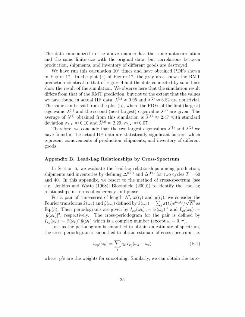
The data randomized in the above manner has the same autocorrelationand the same finite-size with the original data, but correlations betweenproduction, shipments, and inventory of different goods are destroyed.

We have run this calculation 105 times and have obtained PDFs shownin Figure 17. In the plot (a) of Figure 17, the gray area shows the RMTprediction identical to that of Figure 4 and the dots connected by solid linesshow the result of the simulation. We observe here that the simulation resultdiffers from that of the RMT prediction, but not to the extent that the valueswe have found in actual IIP data, λ(1) ≈ 9.95 and λ(2) ≈ 3.82 are nontrivial.The same can be said from the plot (b), where the PDFs of the first (largest)eigenvalue λ(1) and the second (next-largest) eigenvalue λ(2) are given. Theaverage of λ(1) obtained from this simulation is λ(1) ≈ 2.47 with standarddeviation σλ(1) ≈ 0.10 and λ(2) ≈ 2.29, σλ(2) ≈ 0.07.

Therefore, we conclude that the two largest eigenvalues λ(1) and λ(2) wehave found in the actual IIP data are statistically significant factors, whichrepresent comovements of production, shipments, and inventory of differentgoods.

Appendix B. Lead-Lag Relationships by Cross-Spectrum

In Section 6, we evaluate the lead-lag relationships among production,shipments and inventories by defining ∆(SP) and ∆(PI) for two cycles T = 60and 40. In this appendix, we resort to the method of cross-spectrum (seee.g. Jenkins and Watts (1968); Bloomfield (2000)) to identify the lead-lagrelationships in terms of coherency and phase.

For a pair of time-series of length N ′, x(tj) and y(tj), we consider theFourier transforms x(ωk) and y(ωk) defined by x(ωk) =

∑j x(tj)e

iωktj/√N ′ as

Eq.(3). Their periodograms are given by Ixx(ωk) := |x(ωk)|2 and Iyy(ωk) :=|y(ωk)|2, respectively. The cross-periodogram for the pair is defined byIxy(ωk) := x(ωk)

∗ y(ωk) which is a complex number (except ω = 0, π).Just as the periodogram is smoothed to obtain an estimate of spectrum,

the cross-periodogram is smoothed to obtain estimate of cross-spectrum, i.e.

sxy(ωk) =∑`

γ` Ixy(ωk − ω`) (B.1)

where γ`’s are the weights for smoothing. Similarly, we can obtain the auto-

25

spectra, sxx and syy. Then, the ratio defined as

κ2xy(ωk) =|sxy(ωk)|2

sxx(ωk) syy(ωk)(B.2)

is the estimate of squared coherency. It satisfies the following inequality:

0 ≤ κ2xy(ωk) ≤ 1, (B.3)

with 0 corresponding to no linear dependence and 1 corresponding to exactlinear dependence of the two time-series at frequency ωk.

The cross-spectrum can be expressed in terms of its amplitude and phaseas follows:

sxy(ωk) = |sxy(ωk)| e2πiφxy(ωk). (B.4)

The phase φxy(ωk) estimates the lead-lag relationship between the series.Note that the estimate of the phase becomes meaningless when the cross-spectrum is small in its amplitude.

In the following estimation, we consider the multiple time-series consistingof the first two components, namely wα,g(tj) =

∑2n=1 an(tj)V

(n)α,g , averaged

over the index g of goods for α = 1, 2, 3. We take two pairs of shipmentsand production (α = (2, 1)), and production and inventory (α = (1, 3))for x(tj) and y(tj). For the smoothing of the cross-periodograms, we useda modified Daniell kernel for the weight γ` of length 11 (corresponding tothe bandwidth ∆ω/2π = 0.01226 cycles per month) with no tapering. Thestandard formulae of significance levels and confidence intervals are used inthe calculation (Bloomfield, 2000).

Figure 18 shows the estimates of κ2xy(ω) and φxy(ω) for the pair (SP) ofshipments and production (panel (a)) and for the pair (PI) of productionand inventory (panel (b)). For κ2xy(ω), the confidence levels (90% and 99%)are depicted by dotted horizontal lines, which are calculated under the nullhypothesis of zero coherency at each frequency. The estimate of κ2xy and its95% confidence interval are shown by a curve and the shaded region aroundit. One can then see that κ2xy is significant at all frequencies for the pair(SP), while it is significant only at low frequencies corresponding to T & 20months for the pair (PI).

In the frequency regions where the squared coherency κ2xy(ω) is signifi-cant, one can evaluate the phase and its confidence interval in each plot ofφxy(ω). We examine the sign and magnitude of the phase to evaluate the

26

lead-lag relationship and its magnitude. For the pair of (SP), at the twofrequencies ωk=6, ωk=4 corresponding to T = 40, 60 months, respectively, thephase is significantly positive meaning that shipments lead production atthese frequencies. Its magnitude can be evaluated in months by calculatingφxy(ω)/ω and its confidence intervals. The results are

∆(SP)40 = 2.26 [1.43, 3.09], ∆

(SP)60 = 2.74 [0.973, 4.49], (B.5)

where the square brackets represent 95% confidence intervals. For the sakeof comparison, in Figure 18, the results presented in Section 6 are depictedas two points with error bars at T = 40, 60 in the plot of φxy(ω).

For the pair of (PI), the technique of alignment (Jenkins and Watts, 1968)was used to weaken the biasing effect due to rapidly changing phase in thepresence of large lead-lag. The two series of production and inventory arealigned by translating one series a distance of 8 months so that the peak inthe cross-correlation function of the aligned series is close to zero lag. Thenthe results are

∆(PI)40 = 9.04 [7.86, 10.2], ∆

(PI)60 = 9.32 [7.56, 11.1]. (B.6)

Just at in panel (a) of Figure 18, in panel (b) for the pair of (PI), theresults presented in Section 6 are depicted as two points with error bars in theplot of φxy(ω). The confidence intervals do not overlap with the error bars,presumably due to the alignment problem, but we found no large differencesfrom the results.

It is interesting to compare the above results based on two extracted eigen-modes, namely our “business cycles”, with the cross-spectrum for the originaldata, that is, by retaining all the eigenmodes. Figure 19 shows the estimatesof the cross-spectrum for the original data: (a) for the pair of (SP) and (b)for that of (PI). One can make the following observations for T = 40, 60.

• The squared coherency κ2xy(ω) is significant for both pairs. However,

the phase φxy(ω) is significant for the pair (PI) with a similar magnitudeof phase, whereas for the pair (SP), it is not significantly different fromzero at those periods T .

This observation demonstrates that our extraction of two dominant eigen-modes by the method of RMT is essential to reveal the lead-lag relationshipbetween shipments and production which is not clearly present in the original

27

data. We also note that the extraction does not deform the other results ofsignificant coherency and the lead-lag relationship between production andinventory.

We conclude that the method of cross-spectrum and that used in Section 6are consistent in the evaluation of lead-lag relationships among production,shipments and inventory, and also that the extraction of two dominant eigen-modes or our definition of “business cycles” is essential for understanding thelead-lag relationship between shipments and production.

28

Figure 1: A sample of the IIP data for g = 1 (Manufacturing Equipment).Note: The upper panel shows the indices Sα,1(t) while the lower panel shows the cor-responding growth-rates rα,1(tj) defined by Eq.(1). As explained in the legend, α = 1(Production) is shown by open circles connected by solid lines, α = 2 (Shipment) is shownby open squares connected by dashed lines, and α = 3 (Inventory) is shown by rectanglesconnected by dotted lines. The horizontal axis shows the months beginning January 1988through December 2007.

29

Figure 2: The average power spectrum p(ω) of the normalized growth rate.Note: The horizontal axes is chosen to be the period, T := 2π/ω, which is shown in unitsof months at the bottom and in units of years at the top. The points connected by solidlines (with darker shading) are the spectrum for the seasonally-adjusted data, while thepoints connected with dashed lines (with lighter shading) are for the non-adjusted originaldata.

30

Figure 3: Demonstration of robustness of the T = 60 and T = 40 cycles.Note: The big circles connected with solid lines (denoted as “Original FT” on the topline of the legend) are the spectrum for the seasonally-adjusted data, the same as inFigure 2. The small circles connected with dashed lines (denoted as “Chopped FT” onthe second line of the legend) are the results of the discrete Fourier transformation of thefirst S months as in the manner of Eq. (6). The dark shaded area shows the result of thecontinuous Fourier transform allowing ω to take any value in Eq. (6).

31

Figure 4: PDF of the eigenvalues (bars) and the RMT prediction ρ(λ) (dashed curve).

32

Figure 5: The components of the two dominant eigenvectors, V (1,2).Note: The horizontal axis shows the 21 goods (g = 1, 2, . . . , 21). The gray bars are theproduction (α = 1), the white bars the shipments (α = 2), and the black bars the inventory(α = 3).

33

Figure 6: Power spectrum for the total and the two largest eigenmodes.Note: The solid lines at the top show the power spectrum, which is the same as the solidlines with darker shading in Figure A.2. (Note that the vertical axis is in linear scale inthis plot.) The darker shading show the power spectrum of the first eigenmode, while thelighter shading show that of the second eigenmode.

34

Figure 7: The relative contribution of the two largest eigenmodes to the power spectrum.Note: The relative contributions are the values averaged for each bin. The shading is thesame as in Figure 6. The point A on the horizontal is at T ≈ 38 months.

35

Figure 8: The T = 60 (left) and T = 40 (right) oscillations due to the first eigenvector(top), the second eigenvector (middle), and their sum (bottom).Note: The solid line shows the production averaged over 21 goods, the dashed line theaverage shipments, and the dotted line the average inventory.

36

Figure 9: PDF of the three largest eigenvalues obtained by the simulation.Note: The three vertical lines show the RMT boundary, the value of the true λ(2), andthe value of the true λ(1) in the ascending order.

37

Figure 10: PDF of the time delays obtained by the simulation of 105 times.

Note: (a) ∆(SP)60 (solid lines) and ∆

(SP)40 (dashed lines with gray shading). (b) ∆

(PI)60 (solid

lines) and ∆(PI)40 (dashed lines with gray shading). The vertical line in each plot shows the

observed values. The fact that the simulation results are distributed around the observedvalues is an evidence that the observed values are independent from the noise part andare statistically significant. The statistical measures obtained in this simulation are givenin Table 2.

38

Figure 11: Comparison between the extracted business cycles and the original data.Note: (a) Sum of the T = 60, 40 components of the first and the second eigenvectorsfor production, shipments and inventory, each of which is averaged over 21 goods. (b)The original data shown in the bottom panel are smoothed out by taking one-year simplemoving average. We observe that the systematic “business cycles” are well extracted fromthe original data. (Since the Fourier components of T = 120 and 240 are NOT included inthe plot (a), that part of the the behavior of the real data shown in (b) is not reproducedin the plot (a).)

39

Figure 12: The 2008–09 recession.Note: The IIP data for g = 1 (Manufacturing Equipment) shown in Figure 1 is extendedto encompass the 2008–09 economic crisis. The gray shaded zone depicts the in-sampleperiod used in the analyses in Sections 3–6. Production and shipments almost overlapwith each other and are hard to distinguish.

40

Figure 13: Decomposition of volatility of the extended IIP data.Note: (a) The total volatility. (b) The partial contribution of the first eigenmode to thetotal volatility. (c) The partial contribution of the second eigenmode. The gray shadedzone depicts the in-sample period used for determining the dominant modes.

41

Figure 14: Relative contributions of (a) the largest mode and (b) the second largest mode.Note: Panels (a) and (b) correspond to panels (b) and (c) in Figure 13, respectively.

42

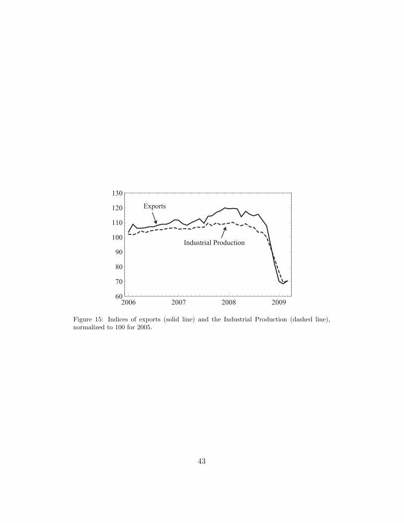
Figure 15: Indices of exports (solid line) and the Industrial Production (dashed line),normalized to 100 for 2005.

43

Figure 16: Autocorrelation of the IIP growth rate, Rα, defined by Eqs.(A.1) and (A.2).

44

Figure 17: Results of the random-ordering simulation.Note: Because of the fact that the IIP data is of finite size and have nontrivial autocor-relation, the distribution of eigenvalues could differ from that of RMT prediction, even ifthe IIP data lacks any comovements. The plot (a) shows that the PDF of the eigenvaluesλ, where the gray-shaded area is the RMT result and the dots connected by lines showthe result of the simulation. The plot (b) shows the PDF of the first eigenvalue λ(1) andthe second eigenvalue λ(2) obtained by simulation. From these, we conclude that λ(1) andλ(2) found in the actual data are in fact principal factors that correspond to comovements.

45

(a)

(b)

Figure 18: Cross-spectrum for the sum of two dominant eigenmodes; (a) for productionand shipments and (b) for production and inventory.

Note: In each plot, κ2xy(ω) is the squared coherency, and φxy(ω) is the phase of the cross-spectrum. In both panels, the dotted lines are 90% and 95% confidence levels for κ2xy(ω)obtained by the null hypothesis of κ2xy(ω) = 0. The gray areas represent 95% confidenceintervals in each plot.

46

(a)

(b)

Figure 19: Cross-spectrum for the original time-series; (a) for production and shipmentsand (b) for production and inventory.

Note: φxy for the production and shipments is not significantly different from zero atT = 40, 60 in the plot of of upper panel. On the other hand, in the lower panel, productionleads inventory by a significant difference in the phase.

47

Table 1: Classifications of 21 goods in IIP.

Final Demand Goods

Investment Goods

Capital Goods 1 Manufacturing Equipment

2 Electricity

3 Communication and Broadcasting

4 Agriculture

5 Construction

6 Transport

7 Offices

8 Other Capital Goods

Construction Goods 9 Construction

10 Engineering

Consumer Goods

Durable Consumer 11 House Work

Goods 12 Heating/Cooling Equipment

13 Furniture & Furnishings

14 Education & Amusement

15 Motor Vehicles

Non-durable 16 House Work

Consumer Goods 17 Education & Amusement

18 Clothing & Footwear

19 Food & Beverage

Producer Goods

20 Mining & Manufacturing

21 Others

Note: The center column is the identification number, g.

48

Table 2: Simulation results on the time delays in comparison with estimates based on theoriginal data.Note: σ is the standard deviation, and “95% CI” is the Confidence Interval at the 95% ofthe distribution of the simulation results shown in Figure 10.

Original data Average σ 95% CI

∆(SP)60 4.28 4.16 1.22 [ 2.17, 6.91 ]

∆(SP)40 1.93 1.87 0.77 [ 0.57, 3.57 ]

∆(PI)60 10.95 11.07 2.25 [ 6.92, 15.77 ]

∆(PI)40 13.62 13.67 2.00 [ 9.94, 17.78 ]

49

Footnotes

1. Shapiro and Watson (1988) consider labor supply shocks as well astechnology shocks, and obtain the “surprising” result that the laborsupply shocks account for at least 40 percent of output variation atall horizons. However, Hall (1988) shows that this finding is neithersurprising nor plausible. Specifically, as Hall criticizes, Shapiro andWatson (1988) make the implausible identifying assumption that allthe contemporaneous comovements of output and work hours be at-tributed to shifts in labor supply, and rule out the alternative assump-tion, perhaps more plausible to many, that the moving force operatesfrom output to hours in the short-run. This paper indeed demonstratesthat output is basically determined by real demand in business cycles.

2. This reduces the number of independent real components in the com-plex Fourier coefficients w’s from 2N ′ − 1 down to N ′, guaranteeingthat the Fourier coefficients w’s are the faithful representation of theoriginal series w.

3. The seasonal adjustment is done by the U.S. Census Bureau’s X-12ARIMA method. The details are given in the resources available fromMETI, Japan (2008).

4. Note that the vertical scale in Figure 2 is logarithmic.

5. There are, in fact, slight dips at those frequencies, which means thatthe seasonal adjustments are somewhat excessively done. However, wehave also looked at the auto-correlation of the data and have foundthat the adjusted data is much better than that of the non-adjusteddata. The relevant results are available from authors upon request.

6. These variables must be normally distributed and uncorrelated.

7. We note that our extraction of the first two dominant eigenmodes isessential for obtaining the lead-lag relationship between shipments andproduction. In fact, if we use all the eigenvectors, which is equivalentto the usual Fourier decomposition, we obtain −0.10 months insteadof 4.28 months in Eq.(32) and 0.34 months instead of 1.93 months inEq.(34). They are much smaller than our time-increment of 1 month,and therefore, are too small to be taken as being significantly differentfrom zero.

50

References

Aoki, M., Yoshikawa, H., 2002. Demand saturation-creation and economicgrowth. Journal of Economic Behavior & Organization 48, 127–154.

Bai, J., Ng, S., 2002. Determining the number of factors in approximatefactor models. Econometrica 70, 191–221.

Blanchard, O., Quah, D., 1989. The dynamic effects of aggregate demandand supply disturbances. American Economic Review 79, 655–673.

Blinder, A., Maccini, L., 1991. Taking stock: a critical assessment of recentresearch on inventories. Journal of Economic Perspectives 5, 73–96.

Bloomfield, P., 2000. Fourier Analysis of Time Series: An Introduction. JohnWiley & Sons. second edition.

Bouchaud, J., Potters, M., 2000. Theory of financial risks: from statisticalphysics to risk management. Cambridge University Press.

Buja, A., Eyuboglu, N., 1992. Remarks on parallel analysis. MultivariateBehavioral Research 27, 509–540.

Cattell, R., 1966. The scree test for the number of factors. Multivariatebehavioral research 1, 245–276.

Diebold, F., Rudebusch, G., 1990. A nonparametric investigation of durationdependence in the American business cycle. Journal of Political Economy98, 596–616.

Francis, N., Ramey, V., 2005. Is the technology-driven real business cyclehypothesis dead? Shocks and aggregate fluctuations revisited. Journal ofMonetary Economics 52, 1379–1399.

Granger, C., 1966. The typical spectral shape of an economic variable. Econo-metrica 34, 150–161.

Guttman, L., 1954. Some necessary conditions for common-factor analysis.Psychometrika 19, 149–161.

Haberler, G., 1964. Prosperity and Depression. New edition. First publishedby the League of Nations. Cambridge, Mass. Harvard University Press[1937] 408, 167–87.

51

Hall, R., 1988. Comment on Shapiro and Watson. NBER MacroeconomicsAnnual 3, 148–151.

Hicks, J., 1950. A Contribution to the Theory of Trade Cycle. OxfordUniversity Press.

Horn, J., 1965. A rationale and test for the number of factors in factoranalysis. Psychometrika 30, 179–185.

Hornstein, A., 1998. Inventory Investment and the Business Cycle. FederalReserve Bank of Richmond Economic Quarterly 84, 49–71.

Jackson, J., 1991. A user’s guide to principal components. Wiley-Interscience.

Jenkins, G., Watts, D., 1968. Spectral Analysis and its Applications. Hoden-Day, San Francisco.

Jolliffe, I., 2002. Principal component analysis. Springer verlag.

Kaiser, H., 1960. The application of electronic computers to factor analysis.Educational and psychological measurement 20, 141.

Kydland, F., Prescott, E., 1982. Time to build and aggregate fluctuations.Econometrica 50, 1345–1370.

Lucas, J.R., 2003. Macroeconomic priorities. American Economic Review93, 1–14.

Mankiw, N., 1989. Real business cycles: A new Keynesian perspective. Jour-nal of Economic Perspectives , 79–90.

Marcenko, V., Pastur, L., 1967. Distribution of eigenvalues for some sets ofrandom matrices. Mathematics of the USSR-Sbornik 1, 457.

METI, Japan, 2008. Indices of Industrial Production, Producer’s Shipments,Producer’s Inventory of Finished Goods and Producer’s Inventory Ratioof Finished. http://www.meti.go.jp/english/statistics/tyo/iip/index.html.

Metzler, L., 1941. The nature and stability of inventory cycles. The Reviewof Economics and Statistics 23, 113–129.

Mitchell, W., 1951. What happens during Business Cycles: A Progress Re-port. National Bureau of Economic Research.

52

Ormerod, P., 2008. Random Matrix Theory and the Evolution of Busi-ness Cycle Synchronisation, 1886–2006. Economics: The Open-Access,Open-Assessment E-Journal 2. http://www.economics-ejournal.org/

economics/discussionpapers/2008-11.

Peres-Neto, P., Jackson, D., Somers, K., 2005. How many principal com-ponents? Stopping rules for determining the number of non-trivial axesrevisited. Computational Statistics and Data Analysis 49, 974–997.

Samuelson, P., 1939. Interaction between the multiplier analysis and theprinciple of acceleration. The Review of Economics and Statistics 21, 75–78.

Sargent, T., Sims, C., 1977. Business Cycle Modeling without pretending tohave too much a priori Economic Theory. New Methods in Business CycleResearch 1, 145–168.

Shapiro, M., Watson, M., 1988. Sources of business cycle fluctuations. NBERMacroeconomics annual 3, 111–148.

Slutzky, E., 1937. The summation of random causes as the source of cyclicprocesses. Econometrica 5, 105–146.

Stock, J., Watson, M., 1998. Diffusion indices. NBER working paper 6702.

Stock, J., Watson, M., 2002. Forecasting using principal components from alarge number of predictors. Journal of the American Statistical Association97, 1167–1179.

Summers, L., 1986. Some skeptical observations on RBC theory. FederalReserve Bank of Minneapolis Quarterly Review 10, 23–27.

Tobin, J., 1993. Price flexibility and output stability: an old Keynesian view.Journal of Economic Perspectives 7, 45–65.

Wigner, E., 1955. Characteristic vectors of bordered matrices with infinitedimensions. Annals of Mathematics 62, 548–564.

Zwick, W., Velicer, W., 1986. Comparison of five rules for determining thenumber of components to retain. Psychological Bulletin 99, 432–442.

53