4. WGS 84 ELLIPSOIDAL GRAVITY FORMULA

4.1 General

In Section 3.1, the WGS 84 Ellipsoid is identified as being a

geocentric equipotential ellipsoid of revolution. An equipotential

ellipsoid is simply an ellipsoid defined to be an equipotential surface,

i.e., a surface on which all values of the gravity potential are equal.

Given an ellipsoid of revolution, it can be made an equipotential surface

of a certain potential function, the theoretical (normal) gravity

potential (U). This theoretical gravity potential can be uniquely

determined, independent of the density distribution within the ellipsoid,

by using any system of four independent constants as the defining

parameters of the ellipsoid. As noted earlier for the WGS 84 Ellipsoid

(Chapter 31, these are the semimajor axis (a), the normalized second

degree zonal gravitational coefficient ( , the earth's angular 2,o

velocity ( w ), and the earth's gravitational constant (GM).

To determine the theoretical gravity potential without resorting

to the use of a mass distribution model for the ellipsoid, U can be

expanded into a series of zonal ellipsoidal harmonics of linear 1/2

eccentricity in (a2 - b2) . The coefficients in the series are

determined by using the condition that the ellipsoid (Chapter 3) is an

equipotential surface

U = Uo = Constant . (4-1)

Since all the zonal ellipsoidal harmonic coefficients vanish, except the

two of degree zero and two, a closed finite expression is obtained for U

C4.1; pp 64-66].

Theoretical gravity ( y ) , the gradient of U, is given on (at) the surface of the ellipsoid by the closed formula of Somigliana [4.1; p 701:

2 2 2 2 'I2 (4-2) y = (a ye cos 4 + b Y sin $)/(a cos 4 + b sin m) P

where

a, b = semimajor and semiminor axes of the ellipsoid, respectively

y y = theoretical gravity at the equator and poles, e' P

respectively

$J = geodetic latitude.

Thus, the equipotential ellipsoid serves not only as the reference surface

or geometric figure of the earth, but leads to a closed formula for

theoretical gravity at the ellipsoidal surface.

4.2 Analytical and Numerical Forms

4.2.1 Formulas

The closed gravity formula of Somigliana in the form C4.21

2 2 2 1/2 'f = ye (1 + k sin ) ) / ( I - e sin $J)

has been selected as the official WGS 84 Ellipsoidal Gravity Formula. In

Equation (4-3):

ez = square of the first eccentricity of the ellipsoid.

Equation (4-3) was selected for use with WGS 84 in preference to Equation

(4 -2 ) since it cs more convenient for ~~jrn~rical -wputatj$ns

explicitly contains ye as the first factor in the equation.

The WGS 84 Ellipsoidal Gravity Formula, expressed

numer i ca 1 ly, is

where

ye= 9.7803267714 rn s - ~

ye= 978.03267714 cm s-2 (Gals)

= 978032.67714 milligals.

In the preceding:

1 Gal = an acceleration due to gravity of 1 centirneter/second

squared

1 milligal = an acceleration due to gravity of 1 x

centimeters/second squared.

4.2.2 Derivation

Several geometric and physical constants derived from the

defining parameters of the WGS 84 Ellipsoid are needed in transforming the

analytical expression for the WGS 84 Ellipsoidal Gravity Formula, Equation

(4-3), to numerical form, Equation (4-5). The fundamental derived

geometric constant is e2, which is related to the four defining parameters

o f t h e WGS 84 E l l i p s o i d v i a Equat ion (3-24). Equat ion (3-24), repeated

here f o r convenience,

i s so l ved i t e r a t i v e l y f o r e2, t a k i n g i n t o account

and t h e f o l l o w i n g express ion f o r t h e second

Wi th t h e d e r i v e d geometr ic cons tan t e2 a v a i

e '

e c c e n t r i c i t y ( e l 1:

(4-8)

lab le , another needed geometr ic

constant , t h e semiminor a x i s o f t h e e l l i p s o i d ( b ) , can be d e r i v e d us i ng

t h e express ion C4.21:

By v i s u a l l y i n s p e c t i n g Equat ions (4-3) and (4-41, it i s

apparent t h a t t h e d e r i v e d p h y s i c a l cons tan ts needed t o complete t h e numer-

i c a l development o f t h e WGS 84 E l l i p s o i d a l G r a v i t y Formula a re y e and

Y ~ ' t h e va lues o f t h e o r e t i c a l g r a v i t y on ( a t ) t h e su r f ace o f t h e e l l i p s o i d

a t t h e equator and t h e poles, r e s p e c t i v e l y . Knowing t h e d e f i n i n g param-

e t e r s o f t h e WGS 84 E l l i p s o i d , and w i t h t h e d e r i v e d geometr ic cons tan ts

e2, e and b a v a i l a b l e , Equat ions (3-65), (3-66), and t h e f o l l o w i n g

Equat ion (4-10) can be used t o compute q:, qo, and m, r e s p e c t i v e l y :

These r e s u l t s a re then used i n

numer ica l va lues f o r y e and y . P

The ana l y t i c a 1

(4-10)

Equat ions (3-63) and (3-64) t o o b t a i n

and numer ica l forms of t h e WGS 84

E l l i p s o i d a l G r a v i t y Formula a re p rov i ded i n Table 4.1. The WGS 84

4 - 4

Ellipsoidal Gravity Formula, numerical form, and the WGS 84 Ellipsoid-

related defining and derived parameters used in its determination are

provided in Table 4.2. For user convenience, values of theoretical

gravity on the surface of the WGS 84 Ellipsoid are provided in Table 4.3 at lo intervals of geodetic latitude. These values, in milligal (mgal)

units, were computed using Equation (4-5).

4.3 Average Value of Theoretical Gravity ( 7 )

4.3.1 Average Value (WGS 84 Ellipsoid)

A number of formulas used in gravimetric geodesy

applications require an average value of theoretical gravity. The average

value of theoretical gravity for the WGS 84 Ellipsoid is

- Y = 979764.46561 milligals. (4-11)

(Although many texts represent the average value of theoretical gravity by

G, that symbol is not used here since it is already used to denote the

universal gravitational constant and also appears in GM.

4.3.2 Derivation of 7 (WGS 84 Ellipsoid)

The general equation for calculating the average value of

theoretical gravity for the earth is

y = Ivds / I I d s S S

where

y = value of theoretical gravity

S = surface of the earth

ds = surface element.

For a rotational el 1 ipsoid, Equation (4-12) becomes

= I J Y RMRN COS( d+ dA / J RMRN COS+ d+ dA (4-13) A 4 A +

where

RM = radius of curvature in the meridian

RN = radius of curvature in the prime vertical

a = semimajor axis

e = first eccentricity.

Upon inserting the expressions for RM and RN into Equation

(4-131, considering that neither they nor theoretical gravity ( y ) are a

function of longitude, and considering the symmetry of these functions -

with respect to the equator, the expression for Y becomes C4.21:

In order to evaluate this equation, both y and (1 - e2sin2+)-2 are

expanded in a series and the resultant equation integrated term by term.

Inspecting the denominator of Equation (4-161,

"I2 cos+ d+ .rr/ 2 I 2 2 -2 = I (1 - e sin +) cos+ d+ , (4-17) o (I - eZsin2+)2 o

it is noted that a series expansion is needed for the expression 2 2 -2 (1 - e sin +) . In series form:

2 2 -2 2 2 4 4 6 6 8 8 ( 1 - e s i n 4) = 1 + 2e s i n @ + 3e s i n @ + 4e s i n 4 + 5e s i n 4 + ...

(4- 18 1

I n s e r t i n g Equat ion (4-18) i n t o (4-17) and pe r f o rm ing t h e i n t e g r a t i o n :

.rr/ 2 2 2 i ( 1 - e s i n cosm ci+ = 1 + l e 2 + - Z e 4 + 4 e6 + ? e8 + ...

Since t h i s r e s u l t rep resen ts t h e denominator o f t h e equa t ion f o r t h e mean

va lue o f t h e o r e t i c a l g r a v i t y , Equat ion (4-161, i t s r e c i p r o c a l must be

determined. The r e c i p r o c a l i s

To eva lua te

i t i s necessary t o have a 2 2 -2 ( y ) a n d ( 1 - e s i n 4 1 .

t h e o r e t i c a l g r a v i t y [4.21,

t h e numerator o f Equat ion (4-161,

7r/2 2 2 -2 = Y ( 1 - e s i n 4) cosm d+ , 0

s e r i e s expansion f o r bo th t h e o r e t i c a l g r a v i t y

Using t h e t r u n c a t e d s e r i e s expansion f o r

2 4 6 8 Y = y e l l + a2 s i n 4 + a s i n 4 + a s i n I$ + a8 s i n q~) 4 6

and Equat ion (4-181, leads t o

d 2 1 Y (1 - e2sin2m)-* cosm dm

2 2 4 4 6 6 8 8 . ( 1 + 2e s i n 4 + 3e s i n q~ + 4e s i n $ + 5e s i n +) cosm d @ .

Th i s express ion can be w r i t t e n as:

n/ 2 2 2 / ~ ( 1 - e s i n cosm dm 0

a/ 2 5 2 2 35 e4 = Ye J [l + I- e + k ) s i n + + (- 4

+ 5 e2k) s i n $ 0 8 8 2

105 ,6 35 4 + (-

6 + - e k ) s i n (p + (- 105 6 8 e8 + - e k ) s i n $1 cosm d$ 16 8 128 16

Combining t h e express ions f o r t h e numerator and

denominator, Equat ions (4-21) and (4-20), r e s p e c t i v e l y , t h e equa t ion f o r

c a l c u l a t i n g t h e mean va lue o f t h e o r e t i c a l g r a v i t y over a r o t a t i o n a l

e l l i p s o i d i s

where y , e2, and k a re de f i ned as before. e

2 Using Equation (4-22) and values for ye, e , and k from

Table 4.1, the average value of theoretical gravity for the WGS 84

Ellipsoid was computed. This value was provided earlier as Equation

(4-11).

4.4 Atmospheric Effects

4.4.1 Theoretical Considerations

In the discussion on the equipotential ellipsoid

(Section 3.21, it was stated that the reference ellipsoid "is defined to

enclose the whole mass of the Earth, including the atmosphere". This, of

course, results from the adoption of a GM value which includes the mass of

the atmosphere. As a result, the theoretical gravity formula derived for

WGS 84 is for an ellipsoid that includes the mass of the atmosphere. This

permits the theoretical gravity field to be computed at the ellipsoid

surface and in space without having to consider the variation in atmospheric density.

Use of a GM value, in the development of the theoretical gravity formula, that includes the mass of the atmosphere is a deviation

from what was done in the development of previous world geodetic system

ellipsoidal gravity formulas. Therefore, caution must be exercised when

using the WGS 84 Ellipsoidal Gravity Formula to ensure that it is

implemented correctly. For those situations which require that

atmospheric effects be considered, this is done by applying corrections to

the measured values. Therefore, the burden of taking atmospheric effects

into account is transferred from the reference system to the gravity data

measurement/reduction process.

4.4.2. Atmos~heric Correction to Measured Gravitv

In the IAG publication on Geodetic Reference System 1967

[4.31, a detailed derivation is given of the correction to measured

gravity for the effect of the earth's atmosphere. The publication also

c o n t a i n s a t a b l e of atmospher ic c o r r e c t i o n values, 6gA, which a re t o be

added t o measured g r a v i t y , when g r a v i t y anomal ies a re be ing formed. Three

s e t s o f BgA va lues a r e g i ven i n t h e t a b l e :

- Values c a l c u l a t e d t o 1 x m s - ~ o r 0.001 mgal),

us i ng t h e Committee f o r Space Research (COSPAR) I n t e r n a t i o n a l Reference

Atmosphere (CIRA 1961).

- Values c a l c u l a t e d t o 1 x m ( o r 0.001 mgal),

u s i n g t h e Un i t ed S ta tes Standard Atmosphere.

- The average o f t h e r e s u l t s ob ta i ned us i ng t h e two above

atmospher ic models, rounded t o 1 x m ( o r 0.01 mgal) .

The s e t o f average atmospher ic c o r r e c t i o n s was recommended

by t h e I A G f o r use w i t h bo th GRS 67 and GRS 80 . For cons is tency, t h i s

s e t i s a l s o recommended f o r use when forming WGS 84 g r a v i t y anomalies.

For ease o f re fe rence , t h i s s e t o f atmospher ic c o r r e c t i o n s i s p rov i ded i n

Table 4.4 f o r e l e v a t i o n s up t o 34 k i l ome te r s , a t 0.5 k i l o m e t e r e l e v a t i o n

increments up t o 10 k i l o m e t e r s and a t l a r g e r increments a t h i ghe r

e l e v a t i o n s . These c o r r e c t i o n s a re a l s o d e p i c t e d g r a p h i c a l l y i n

F i g u r e 4.1.

For t hose a p p l i c a t i o n s where use o f Table 4.4 i s

i nconven ien t o r perhaps cumbersome f o r e s t i m a t i n g needed atmospher ic

c o r r e c t i o n values, t h e f o l l o w i n g e m p i r i c a l l y d e r i v e d equa t ion may be used

i n i t s p l ace [4.41:

-0.116 h 1.047 6gA = 0.87 e mgal.

I n Equat ion (4-23), which reproduces Table 4.4 t o an RMS accuracy o f

20.0094 mgal, h i s t h e h e i g h t o f t h e g r a v i t y s t a t i o n above mean sea l e v e l

i n k i l o m e t e r s . Atmospheric c o r r e c t i o n va lues determined f rom Equat ion

(4-23) d i f f e r f r om Table 4.4 va lues by l ess than 0.01 mgal f o r e l e v a t i o n s

up to 10 kilometers, with a maximum difference of 0.0224 mgal, which

occurs when h = 15 kilometers.

As stated above, the atmospheric correction values are to

be added to measured gravity values when the latter are used along with

theoretical gravity (WGS 84 El 1 ipsoidal Gravity Formula) values to obtain

WGS 84 gravity anomalies. The relevant formula is

'gS4 = + &gA- Yg4 + gravity reduction terms (4-24)

where

~g~~ = gravity anomaly referenced to the WGS 84 Ellipsoid,

and of type corresponding to the gravity reduction

terms applied

g = value of gravity measured on the earth's physical

surface (and referenced to the Internat iona 1

Gravity Standardization Net 1971) C4.51

SgA = atmospheric correction to measured gravity (at the

elevation above mean sea level of the gravity

station)

y84 = value of theoretical gravity calculated using the

WGS 84 Ellipsoidal Gravity Formula

and "gravity reduction terms" pertain to the type of gravity reduction

applied (e.g., free-air, Bouguer, etc.).

4.5 Gravity Anomaly Conversion

4.5.1. Recommended Approach

When implementing WGS 84, gravity anomalies referenced to

the WGS 72 Ellipsoidal Gravity Formula, or other in-use ellipsoidal

gravity formulas (International 1930, GRS 67, GRS 80, etc. ), will need to

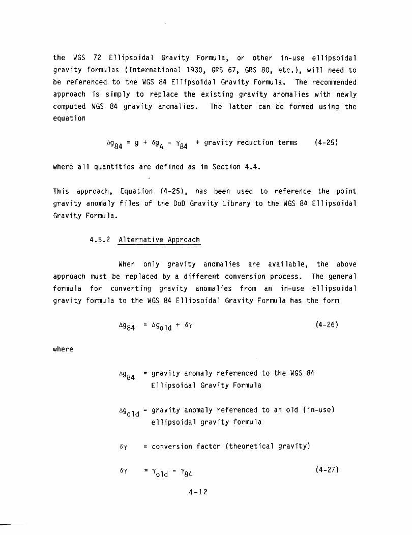
be referenced to the WGS 84 Ellipsoidal Gravity Formula. The recommended

approach is simply to replace the existing gravity anomalies with newly

computed WGS 84 grav equation

ity anomalies. The latter can be formed using the

+ "SA - Ys4 + gravity reduction terms (4-25)

where all quantities are defined as in Section 4.4.

This approach, Equation (4-251, has been used to reference the point

gravity anomaly files of the DoD Gravity Library to the WGS 84 Ellipsoidal

Gravity Formula.

4.5.2 Alternative Approach

When only gravity anomalies are available, the above

approach must be replaced by a different conversion process. The general

formula for converting gravity anomalies from an in-use ellipsoidal

gravity formula to the WGS 84 Ellipsoidal Gravity Formula has the form

where

~g~~ = gravity anomaly referenced to the WGS 84

Ellipsoidal Gravity Formula

= gravity anomaly referenced to an old (in-use)

ellipsoidal gravity formula

6y = conversion factor (theoretical gravity)

Yold = theoretical gravity computed using an old

(in-use) ellipsoidal gravity formula

Y84 = theoretical gravity computed using the WGS 84

Ellipsoidal Gravity Formula.

In Equation (4-26), it is assumed that the measured values of gravity used in forming ngold have been corrected for atmospheric effects (Section 4.4, above). Also, it is apparent from Equation (4-26) that an existing file

of gravity anomalies can be referenced to WGS 84, provided an appropriate

expression is available for 6y .

The WGS 72 Ellipsoidal Gravity Formula, when expressed in International System (SI) units, has the form C4.61:

This formula was developed using a truncated Chebychev polynomial

expansion. Therefore, it is necessary to develop the 6y conversion from

'7 2 to yg4, using the WGS 84 Ellipsoidal Gravity Formula expressed in the form of a truncated series C4.41. Operating with this truncated

series and Equation (4-281, the following equation was developed for use

in Equation (4-26) to convert WGS 72 gravity anomalies to WGS 84 gravity

anomalies:

2 6~ = (0.5929 - 0.0432 sin @ + 0.1851 sin4@ (4-29)

6 8 - 0.1234 sin @ - 0.0007 sin $1 x 10% .

Additional details are available in C4.41 on the development of Equation

(4-29).

Equation (4-29) is listed in Table 4.5 along with

analogous expressions for converting gravity anomalies related to the

GRS 67, GRS 80, and International 1930 Gravity Formulas to the WGS 84

E l l i p s o i d a l G r a v i t y Formula. Unless t h e measured g r a v i t y va lues used i n

fo rm ing t h e o r i g i n a l g r a v i t y anomalies had t h e atmospher ic c o r r e c t i o n

SgA app l ied , t h i s c o r r e c t i o n must now be a p p l i e d as p a r t o f t h e

conversion-to-WGS 84 process. The r e l e v a n t equa t ion i s :

When u s i n g Equa t ion (4-301, i t ' s impor tan t t o r e c a l l t h a t 6gA, Equat ion

(4-23), i s a f u n c t i o n of g r a v i t y s t a t i o n (measurement) e l e v a t i o n above

mean sea l e v e l .

4.6 Comments

As i n d i c a t e d i n Sec t ion 4.5.1, t h e p o i n t g r a v i t y anomaly f i l e s o f

t h e DoD G r a v i t y L i b r a r y have been re fe renced t o t h e WGS 84 E l l i p s o i d a l

G r a v i t y Formula and w i l l be o f f i c i a l l y ma in ta ined on t h a t formula. The

e l l i p s o i d a l g r a v i t y formula convers ion was accompl ished by us i ng t h e p o i n t

g r a v i t y obse rva t i ons ( g ) i n t h e DoD G r a v i t y L i b r a r y F i l e s i n t h e manner

p r e s c r i b e d by Equa t ion (4-25). These newly formed WGS 84 p o i n t g r a v i t y

anomal ies a re be ing used t o generate WGS 84 mean g r a v i t y anomalies f o r t h e

DoD G r a v i t y L i b r a r y f i l e s . Al though t h e f i l e s o f t h e DoD G r a v i t y L i b r a r y

w i l l be r e fe renced t o t h e WGS 84 E l l i p s o i d a l G r a v i t y Formula, DMA w i l l

m a i n t a i n t h e c a p a b i l i t y t o p rov i de reques te rs w i t h p o i n t and mean g r a v i t y

anomal ies r e f e r r e d t o any o f t h e E l l i p s o i d a l G r a v i t y Formulas i d e n t i f i e d

i n Table 4.5.

KEFERENCES

4.1 Heiskanen, W. A. and H. M o r i t z ; P h y s i c a l Geodesy; W. H. Freeman and

Company; San F r a n c i s c o , C a l i f o r n i a ; 1967.

4.2 M o r i t z , H. ; "Geode t i c Reference System 1980" ; Bu l l e t i n Geodesique;

Vol . 54, No. 3; P a r i s , France; 1980.

4.3 Geode t i c Reference System 1967; S p e c i a l P u b l i c a t i o n No. 3;

I n t e r n a t i o n a l A s s o c i a t i o n o f Geodesy; P a r i s , France; 1971.

4.4 D i m i t r i j e v i c h , I.J.; WGS 84 E l l i p s o i d a l G r a v i t y Formula and G r a v i t y

Anomaly Convers ion Equat ions ; Pamphlet; Department o f Defense G r a v i t y

S e r v i c e s Branch; Defense Mapping Agency Aerospace Center ; S t . Lou is ,

M i s s o u r i ; 1 August 1987.

4.5 M o r e l l i , C.; The I n t e r n a t i o n a l G r a v i t y S t a n d a r d i z a t i o n Net 1971

(IGSN 71) ; S p e c i a l P u b l i c a t i o n No. 4; C e n t r a l Bureau, I n t e r n a t i o n a l

A s s o c i a t i o n o f Geodesy; P a r i s , France; 1971.

4.6 Seppe l i n , T.O.; The Department o f Defense World Geodet ic System 1972;

T e c h n i c a l Paper; Headquar ters , Defense Mapping Agency; Washington,

DC; May 1974.

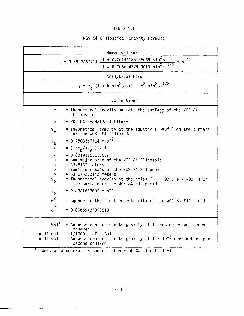
Table 4.1

WGS 84 Ellipsoidal Gravity Formula

Numerical Form

Y = 9.7803267714 1 + 0.00193185138639 sin2+ s-2

(1 - 0.00669437999013 sinZ$) 'lE

Analytical Form

2 2 2 1/2 Y = re (1 + k sin +)/(l - e sin 4)

Definitions

= Theoretical gravity on (at) the surface of the WGS 84 El lipsoid

= WGS 84 geodetic latitude

= Theoretical gravity at the equator ( $=oO ) on the surface of the WGS 84 Ellipsoid

= ( bvp/aue - 1 = 0.00193185138639 = Semimajor axis of the WGS 84 Ellipsoid = 6378137 meters = Semiminor axis of the WGS 84 Ellipsoid = 6356752.3142 meters = Theoretical gravity at the poles ( @ = goU, $ = -goU ) on

the surface of the WGS 84 Ellipsoid

= Square of the first eccentricity of the WGS 84 El lipsoid

Gal* = An acceleration due to gravity of 1 centimeter per second squared

milligal = 1/1000th of a Gal milligal = An acceleration due to gravity of 1 x centimeters per

second squared

* Unit of acceleration named in honor of Galileo Galilei

Table 4.2

The WGS 84 Ellipsoidal Gravity Formula and the Defining and Derived Parameters Used in its Derivation

WGS 84 Ellipsoidal Gravity Formula

y = 9.7803267714 1 + 0.00193185138639 sin2$ m s-* (1 - 0.00669437999013 sin2@)

Parameters Symbo 1 s I Numerical Values

Defining Parameters (WGS 84 El 1 ipsoid)

Semimajor axis

Normalized second degree zonal gravitational coefficient

Earth's angular velocity

Earth's gravitational constant (mass of earth's atmosphere included)

7292115 x 10-l1 rad s'l

3986005 x lo8 m3 s-'

Derived Geometric Constants

Semiminor axis I b First eccentricity squared I e2 Second eccentricity squared 1 el2

2q0 = (1 + 3/e12) (arctan e') - 3/e1 90

' = 3(1 + l/e'2).[1 - (l/el) I 'lo' 90

arctan ell - 1 Derived Physical Constants

m = u 2 a 2 b / ~ ~

Theoretical gravity at the equator

Theoretical gravity at the poles

k = (byp/aue) - 1

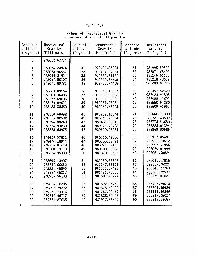
Table 4.3

Values of Theoretical Gravity - Surface of WGS 8 4 Ellipsoid -

;eodet ic -at itude (Degrees)

Theoretical Gravity

(Mi lligals)

Seodet ic Latitude (Degrees)

Theoretical Gravity

(Mi 1 1 igals) 1 Geodetic Latitude (Degrees)

Theoretical Gravity

(Milligals)

Table 4.4

Atmospheric Corrections for Measured Gravity (When Forming WGS 84 Gravity Anomalies)

Elevation Above Mean Sea Level (km)

Correction 6gA(mga 1 )

Elevation Above Mean Sea Level (km)

Correction 6gA(mgal

* Based on the height of the earth's topography, 6gA values for

elevations greater than approximately 9 kilometers (km) above mean sea

level are primarily of academic interest. However, some of the higher

elevation tkjA values may be of practical value in the future if

advances in at-altitude gravity measurement technology continue.

Table 4.5

Equat ions f o r Conver t ing G r a v i t y Anomalies t o t h e WGS 84 E l l i p s o i d a l G r a v i t y Formula

Wor l d Geodet ic System 1972

From

2 4 6y = (0.5929 - 0.0432 s i n + + 0.1851 s i n @

6 8 - 0.1234 s i n 9 - 0.0007 s i n + ) x 1 0 ' ~ m

Conversion Equat ions (Sy) *

Geodet ic Reference System 1980

I n t e r n a t i o n a l 1930

6y = ~0.0000100 + 0.0000196 s i n 2 @ + 0.0000098 s i n 4 +

- 0.0000196 s i n 6 @ - 0.0000293 s i n 8 @ ) x m

Geodet ic Reference System 1967

2 dy = (16.3229 - 13.8426 s i n @ + 0.3214 s i n 4 +

6 8 - 0.1234 s i n + - 0.0007 s i n @ ) x m

2 4 6y = (-0.8271 - 0.1475 s i n + + 0.1860 s i n +

6 8 - 0.1234 s i n + - 0.0007 s i n + ) x m s - ~

Maximum D i f f e r e n c e

0.6138 mgal ( a t + = 68")

0.000018 mgal ** ( a t + = 45")

- 0.9127 mgal ( a t + = 90")

16.3229 mgal ( a t @ = 0")

* These convers ion equa t ions do n o t i n c l u d e a tmospher ic e f f e c t s . (See Sec t ion 4.5.2. )

** Due t o t h e smal lness o f t h e d i f f e r e n c e , t h i s g r a v i t y anomaly convers ion i s unnecessary.

Elevation Above Mean Sea Level (in Kilometers)

Figure 4.1. Atmospheric Correction for Measured Gravity (When Forming WGS 84 Gravity Anomalies)

This page is intentionally blank.