wetlands: methane emissions and spectral...
TRANSCRIPT

•
•
METHANE EMISSIONS FROM THE EASTERN TEMPEPA,TE WETLAND REGION
AND SPECTRAL CHARACTERISTICS OF SUBARCTIC Ff:NS
A thesis submitted to the Faculty of Graduate Studies and I~esearch in partial fulfillment of the requirements for the degre,~ of
Master of Science by
James Windsor
Department of Geography McGill University
Montreal. Quebec April 1993

1
1·
1
WETLANDS: METHANE EMISSIONS AND SPECTRAL CHARACTERISTICS

•
•
Abstract
Resume
Acknowledgments
List of tables and figures
TABLE OF CONTENTS
Chapter 1: Foreword and introductIon
IV
Chapter 2: Methane emissions trom the Eastern Temperate Wetland Region 13
Chapter 3: Spectral characteristics of subarctic fens 45
Summary and Conclusions 67
Literature Cited
Appendix A: Percent reflectance of subarctic fen sites
Appendix B. Mean daily methane flux for Eastern Temperate wetland sItes

•
•
ABSTRACT
Emissions of methane were measured by a static chamber technique at 9 sites
on 5 weflands in the Eastern Temperate Wetland Region, north of Montreal. Mean
daily methane fluxes measured from May to Octobe!" ranged from 0.18 to 1071
mg/m2/d, and estimated an nuai flux ranged from 0.02 to 186 g/m2/y. Laboratory
incubations of peat samples showed potenfial anaerobic methane production rates
which ranged trom 0.00 to 9.12 IJg/g/d, and potential aerobic consumption rates from
0.55 to 3.75 J,Jg/g/d. Seasonal methane emission pattems are related to water table
level and CH4 production and consumption potentials in the peat profile. Episodic
fluxes were found to be important at several sites, contributing a significant portion of
the fotal emissions
Analysis of spectral reflecfance data from 20 sites on 2 subarctic fens was
carned ouI to address the issue of scaling up CH4 emissions using satellite imagery.
Hummocks, lawns and pools were found to be spectrally distinct enough to be
differenfiafed by band 5 of Landsat MSS and band 3 of Landsat TM sensors. The
averaging of spectral information in mixed pixels proved unlikely to be able to
distlnguish between wet lawn and string and pool communities. Such weaknesses can
be overcome with the use of higher resolution data .

• •
•
\1
Le~ dégagements de méthane ont été measures au moyen d'une technique
en enceinte statique aux 9 sites sur 5 marécages dans la Region des Terre:. Humides
Temperées de l'Est au nord de Montréal. Quebec. La moyenne quotidienne des
émissions de méthane qUI ont été measurées entre Mai et Octobre allOient de 0,18 a
1071 mg/m2/j, et les estimations des émissions annuelles allaient de 0,02 à 186 g/m·'/a.
Les incubations des échantillons de tourbe ont révelé des débits de production
anaerobique potentielle ce méthane qui allaient de O,QO à 9,12 \-Ig/g/j. et des de bits
de consommation aerobique potentielle de méthane qui allaient de 0.55 à 3.75
\Jg/g/j. Les phases saisonnières de dégagements de méthane sont reliées au niveau
de la nappe phréatique et des potentielles de production et de consommation de
méthane dans la tourbe. Les dégagements épisodiques etaient Importants a plusieurs
sites et ont contribué considérablement aux émissions totales.
L'analyse des données de reflexion spectrale de 20 sites sur 2 tourbl~res basses
subarctiques a été faite pour addresser la question des estimations des degagements
de méthane régionales en employant les images de satellite. Les buttes, pelouses et
mares sont assez distinctes par charactère spectrale pour être differenciees par la
bande 5 de MSS Landsat et la bande 3 de TM Landsat. Comme l'information
spectrale est fait en moyenne aux pixels des images, il est peu probable que Landsat
puisse faire la distinction entre pelouse mouillée et les tourbières basses stucturees.
Ces limitations du système peuvent être surmontées en utilisant des données de haute
résolution .

•
•
ABSTRACT
Emissions of methane were measured by a static chamber technlqup. at 9 sites
on 5 weflands in the Emtern Temperate Wetland Region, in the Laurentian faothill
region north of Montreal. Mean daily methane fluxes measured from May to October
ranged from 0.18 to 1071 mg/m2/d, and estimated annual flux ranged trom 0.02 to 186
g/m'l/y. Laboratory incubations of peat samples showed potential anaerobic
methane production rates which ranged from 0.00 to 9.12 J,Jg/g/d, and potential
aerobic consumption rates trom 0.55 to 3.75 I-Ig/g/d. Seasonal methane emission
patterns are related to water fable level and CH4 production and consumption
potentials in the peat profile. Episodic fluxes were found to be important at several
sites, contributing a significant portion of the total emissions.
Analysis of spectral 1 eflectance data from 20 sites on 2 subarctic fens was
carried out to address the issue of scaling up CH4 emissions using satellite imagery.
Hummocks, lawns and pools were found to be spectrally distinct enough to be
differentiated by band 5 of Landsat MSS and band 3 of Landsat TM sensors. The
averaging of spectral information in mixed pixels proved unlikely to be able to
distinguish between wet lawn and string and pool communities. Such weaknesses can
be overcome with the use of higher resolution data .

•
•
Il
RESUME
Les dégagements de méthane ont eté mes'Jrés au moyen d'une tec.hnique en
enceinte statique aux 9 site$ sur 5 marecages dans la Region des Terre,> Humldt: s
Temperées de l'Est ou nord de Montréal. Quebec. La moyenne quotidienne de"
émissions de méthane qui ont été measurées entre Mal et Octobre aliOient de 0.18 à
1071 mg/m2/J, et les estimations des emisslom annuelles aliOlenl de 0.02 à 186 g/rw la
Les incubations des échantillons de tourbe ont révelé des deblts de production
anaerobique potentiel de méthane qui allaient de 0,00 à <.J, 12 I-Ig/g/j, et des deblts de
consommation aerobique potentiel de méthane qui allaient de 0,55 à 3.75 I-Ig/g/). 1 es
phases saisonnières de dégagements de méthane sont reliées au niveau de la nappe
phréatique et des potentiels de production et de consommation de méthane dans la
tourbe. Les dégagements épisodiques étaient importants à plusieurs sites et ont
contribué considérablement aux émissions totales.
L'analyse des données de reflexion spectrale de 20 sites sur deux tourbieres
basses subarctiques a été faite pour ad dresser la question des estimations de!>
dégagements de méthane régionales en employant les Images de satellite. Les
buttes. pelouses et mares sont assez distinctes par caractère spectrale pour être
differenciées par la bande 5 de MSS Landsat et la bande 3 de TM Landsat. Comme
l'information spectrale est fait en moyenne aux pixels des images, II est peu probable
que Landsat puisse faire la distinction entre pelouse mOUillée et les tourbières bm!.es
stucturées. Ces limitations du système pelJVent être surmontées en utilisant de,>
données de haute résolutio!l .

• •
•
III
Acn JOWLEDGMFr~TS
For the assistance of Shann0n Glenn, Jill Bubler, Mike Dalva, Monica Bienefeld.
Doug Barr. Andrew Heyes, Anne Bergman, Andrew Castello, Paula Kestelman, Lilian
Lee, Larry Houston and Hardy Granberg in the field and laboratory, 1 wish ta extend
my sincerest gratitude, without the help of these people this project would not exist 1
am 0150 grateful for the staH and facilitles of the University of Montreal Biologlcal
Research Station ln St Hippolyte, Quebec, the McGill Subarctic Research Station ln
SchefferVille, Quebec and the cooperation of Mirabel Alrport for support and oc cess
to study sites. The encouragement and support of the Department of Geography at
MeGIII University IS greatly appreclated, especlally sa the guidance given to me by
Professor Tlm Moore, and the advice and ideas offered by Professors John Lewis and
Michel Lapolnte .

• •
•
1\
LIST OF TABLES AND FIGURES
Figure 1 1 Sources of atmosphenc methane. after Cicerone 5 and Oremland (1988)
Table 1 1 Summary of mean dail methane flux estlmates for 6 wetlands slrrillar to those used ln thls study
Table 2 1. Sites used for methane flux sampling between 14 May and October. thefr type. mean semonal water table position. dominant vegetation. mean semonal methane flux and annual methane flu), estlmate from welghted means.
Figure 2 1 Mean seasonal water table position at Site 1 20
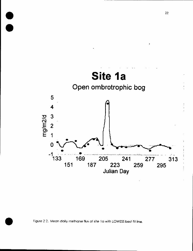
Figure 22 Mean daily methane flux at site 1 a with LOWESS 2~ best fit line
Figure 2.3 Mean dally methane flux at site 1 b wlth a LOWESS ::'3 best fit hne
figure 2.4 Mean dOily methane flux at site 1 c wlth a LOWESS :)4 best fit Ilne.
Figure 2 5. Mean daily methane flux at site 1 d wlth a LOWESS 2S best fit line.
Figure 2 6 Mean daily methane flux at site 2 with a LOWESS 26 best fit line.
Figure 2.7 Mean daily methane flux at site 3 wdh a LOWESS 2/ best fit line
Figure 2 8 Mean daily methane flux at site 4 wlth a LOWESS 28 besf fit line.
Figure 2.9. Mean daily methane flux at site Sa wlth a LOWESS 29 best fit line.
Figure 2.10. Mean dally methane flux at sl<e Sb wlth a 30 LOWES$ best fit line.
figure 2 11 Peat temperature at 20cm for sites 1 0- 1 d 33
Figure 2.12. Methane production potentials from anaeroblc 37 laboratory Incubations

R
• •
•
Figure 2 13 Methane consumption potentials fram aerobic laboratory Incubations.
38
Table 2.2 Summary of CHA production and consumption 39 potentlals. with degree of decomposition for each sample.
Table 3 1. Sites used for spectral reflectance measurement. 48 the heighf at which they were measured and a brief description.
Table 3.2 Percent cover of bryophytes for sites at which 49 reflectance was measured.
Table 3.3. Percent COVE r of vascular species for sites al 50 which reflectance was measured (sites 1-10).
Table 3.4. Percent cover of vascular species for sites at 51 whlch reflectance was measured (sites 11-20).
Figure 3 1 Comparison of reflectance from pool. string and 56 a combination of both sites.
Figure 3.2. Comparison of reflectance from hummock and 58 pool sites.
Figure 3.3. Comparison of reflectance from lawn and pool 59 sites
Figure 3.4. Comparison of reflectance trom various pool 60 sites.
Figure 3 5. Percent reflectance in the range of Landsat TM 63 band 3 and 4 for plots measured trom one metre.
Figure 3.6. Percent reflectance in the range or Landsat MSS 64 band 5 and 6 for plots flleasured from one metre.
FIgure 3.7. Percent reflectance in the range of Landsat MSS 65 band 5 and 7 for plots measured from one metre .
,
•
•
CHAPTER 1
It is broadly befievad that global warming is ta king place. and Ihol
atmospheric gases such as carbon dioxide and rnethane die Imgely
responsible for iL Of 011 the sources of methane on the planet. notural
wetlands are considered to be one of the mosl important (e.g. Matlhews and
Fung 1987, Cicerone and Oremland 1988). Currently, rhere are several
questions dealing with the role of wetlands as a source of atmospheric
methane, and these are pertinent to climate modeling. For example, how
much methane do different wetlands emit~ What faclors control the
magnitude of these emissions? How con we scale this information up to obtain
regional estimates of methane emissions? With reference to sorne specifie
welland communities, if is intended that this thesis will provide sorne answers to
these questions.
Specifie Objectives
The research in this thesis will address a number of iS'iues. As weil as
providing a regional survey of methane flux measurements from wellands
located near Montreal, Quebec, the focus will be on spatial and temporal
variations of methane flux and the contribution of these wetlands to regional
methane emission5. In addition, the control of environmental variables on
magnitude and pattern of methane flux and production will be investigated.
Incubation of peat samples (both aerobic and anaerobic) will be analyzed 10
determine the role of edaphic controls on methane emissions.
Scaling up values of methane emissions to the regional level could be
done if satellite imagery could be used to quantify the areal extent of

• •
•
2
ecologically distinct wetland communities which have different characteristic
values of methane flux. To determine whether such an undertaking is feasible,
one needs to take a closer look ~t the spectral characteristics of these
communities as weil as the strengths and weaknesses of present satellite borne
sensors. Spectral refledance data collected from wetlands in Subarctic
Quebec will be analyzed to address these issues.
These are problems that, once addressed, will help to broaden the data
base of methane flux emissions trom North American wetlands, increase
understanding of the processes and factors controlling methane flux patterns
and magnitude, help to assess the best method of scaling up methane
emission measurements, and increase our understanding of wetland
classification using satellite imagery.
Introduction
A great deal of attention has been paid recently +0 the study of
atmospheric trace gases, due mainly to concern over the so-called
greenhouse effect. Under the greenhouse theory of global warming, it is
hypothesized that increased concentrations of certain gases (such as C02,
CH4 and CFC's) will result in a raising of the earth's temperature by trapping
long wave radiation which would otherwise have escaped to space. As a
result, there is an increase in the energy available to drive the climate sy:;tem,
and as this energy will not be evenly distributed around the globe, changes in
atmospheric and oceanic circulation are likely to occur (Ramanathan 1988).
Of the most important greenhouse gases, C02 has received the most
attention, as it is assumed to have the most impact on global warming at
present (Ramanathan et al. 1985). The result of adding larger quantities of a

• •
•
trace gas to the atmosphere is largely dependent on the CUITent
concentration of the gas; as relatively large concentrations of C02 already
exist in the atmosphere. the effect of adding a given quantity will be less than if
prevailing concentrations were lower. The greater ability of the other trace
gases to absorb radiation cou pied with their presently low atmospheric
concentrations would make increases in their emissions more of a threat to
global warming than that of C02 (Rodhe 1990).
Although the relative contribution of CH4 at cUITent atmospheric
concentrations is less than that of C02. it is about 15 times as efficient at
trapping radiation. If one considers that CH4 concentratiom have nearly
doubled in the last 350 years and continue to increase at approximately 1 %
per year. its importance in the context of climate change becomes obvious
(Ramanathan 1988). A more recent study by Steele F:!t al. (1992) indicates that
there has been a major deceleration in the accumulation of atmospheric
met ha ne between 1983 and 1990. suggesting that the increasing trend may
have come to an end.
A major sink for atmospheric CH4 is oxidation by hydroxyl (OH) radicals in
the troposphere. so increases in concentrations of atmospheric methane mav
bE~ partially due to decreases in tropospheric concentrations of hydroxyl
radicals; it is more likely. however. that rising CHA concentrations are the result
of biological pro cesses (Wang et al. 1986).
Estimates of total global emissions ot methane to the atmosphere range
from 300 to 1490 Tg per year (Moore 1988); most studies agree that 400-600 Tg
per year is more likely (Cicerone and Oremland 1988. Moore 1988. Khalil and
Rasmussen 1990). while others. such as Fung et al. (1991) maintain that this
overestimates actual global emissions. Cicerone and Oremland (1988)
provide a summary of the various sources of global methane emissions and

• •
•
thelr relative Importance (Figure 1.1). They estima te that naturally occurring
wetlands account for over 21 % of global methane emissions, ma king them the
largest single source. Mafthews and Fung (1987) conclude that the global
area covered by naturally occurring wetlands is about 5.3 x 10¹² m2 (it must be
noted that thls estlmate was achieved by integrating digitally collecfed
information averaged over 1 ° cells), and that 60% of the total methane
emissions from wetlands may be aftributed to peat-rich bogs concentrated
between 500 N and 700 N latitude. This concurs with the facf that a sharp
increase in the concentration of tropospheric methane above 500 N (Steele et
al. 1987) coincides with a maximum of wetland distribution between 500 N and
700 N (Aselmann and Crutzen 1989).
There are many problems associated with quantifying the global
methane budget, and attempting to establish the contribution of wetlands
within a reasonable margin ùf error is one of them. Inevitably, there are errors
involved with determining how much of the earth is covered by wetlands, and
considerable difficulty breaking this down into usable units of wetland types.
This is complicated by ambiguity in definitions of wetlands and wetland
boundaries, as weil as a general lack of wetland inventories in many regions of
the world. Assuming this inventory could be completed, one would then need
a database of annual methane emissions from ail types of wetlands which
occur in significant amounts around the globe. To date, many studies of
methane emissions have been do ne in many wetland environments around
the globe. Summarized in table 1.1 are examples of emission estimates
obtained from research carried out in wetlands pertinent to those used for this
study.
Difficulties with obtaining a precise estimate of methane flux from
wetlands result from the great spatial and temporal variability associated with

• •
•
Sources of Atmospheric Methane
Methane hydrate destabilizatlon (0.9%) 1
Freshwaters (0.9%) Oceans (1.9%) \ : i
Coa/ minlng (6.5%) l '1
Landfl/ls (7.4%)
Termites (7 4%)
Gas drU/mg (8 3%)
Blomass burning (10 2%)
Wetlands (21 3%)
Rlce paddles (204%)
Figure 1.1. Sources of atmospheric methane. after Cicerone and Oremfand (1988).

• •
•
6
j'uthor Region study Perlod Wetland Type Mean C H4 Flux (mg m-2 dol)
BLJbler et al. Northern Ontario, May - October Open Bog 5 (In I1re.,~) Canada Treed Bog 5
BeaverPond 392 Conifer Swamp 2 Thicket Swamp 56
Weyhenmeyer 199:2 Central Ontario, June - Odober BeaverPond 37 Canada
Roulel el al. 199'2 Central Ontario, May - Oetober Open Bog 21 Canada Treeo Bog 6
Conifer Swamp 2 BeaverPond 56
Nalman et al. 1991 Minnesota, U.S.A. May - Odober BeaverPond 71
Moore and Southern Quebee. May - November Domed Bog Knowles 1990 Canada
ford and NOiman Quebee. Canada May - Oetober BeaverPond 27 1988
Sebac hel et al. Alaska. U.S.A. August Tundra Bog 3 1986
HailISs el al. 1985 Minnesota. U.S.A. August Perched Bog 132
Svensson and Stordalen. Sweden June - September Open Bog 7 Rosswall 1984
Table 1.1. Summary of mean dail methane flux estimates for wetlands similor to those used in this study .

• •
•
7
methane flux measurement!"i (Moore et al. 1990). insufficlent unders_tandlng of
the environ mental factors controlling methane flux and a lack of data on
different wetland types and their annual methane emissions fBubier et al..
submitted).
Further confusion in determining seasonal emissions may arise" fmm
estimating the relative contribution of episodic fluxes. Such fluxes were found
to occur in subarctic fens during the thawing of upper layers of the peat in
spring, or in the middle of the frost~free season in conjunction with lowering ..)f
the water table (Windsor et al. 1992). As they are of high magnitude and short
duration, there is a reasonable probability of missing such an event dunng the
sampling season; in subarctic fens, this r-esulted in underestimation of semonal
emissions by 7 ~22%.
Dunfield et al. (in press) found that methane production and
consumption in laboratory incubations ot peat samples was sensitive to
changes in pH, with mo~,t samples exhibiting maximum activity up to elbout 2
units above the native pH; the deviation trom native to optimum pH was more
sfrongly pronounced in the more acidic samples. The authors suggest that this
is some indication of adaptation to acidity for the methanogens in the peat
samples used in their study. Williams and Crawford (1985) note that
methanogens, which occupy a very narrow ecological niche dependent on
strict anaerobism. metabolize best in the neutrel pH range of 6.7 to 8.0 when
cultured under laboratory conditions. Having isolated methanogem. trom
ombrotrophic bog water samples, they concluded that such acid-tolerant
methanogens could continue to produce methane at pH values trom 3-4, but
that no growth was detected in this range. Methane production was
consisfently lower at lower pH values for ail cultures studied .

• •
•
Severe! recent studles have investigated the potential for substrate
samples to produce and consume methane under laboratory conditions. often
ln IIght of its importance to methane flux dynamics in wetlands. Svensson and
Rosswall (1984) found that a subarctic peat profile had a CH4 production
maximum at aro~nd 10 cm depth. and little or no production above or below
thls. These results may be misleading. as the head space in the vessel WClS not
sample'd untll a full month after the beginning of the experiment. Soil samples
taken from different depths at an Alaskan tundra meadow were colleded for
loboratory studies on their potential to consume methane (Whalen and
Reeburgh 1990). The authors concluded that methane consumption at depth
was sufficient to decrease net methone fluxes in these soils. and that tundra
moy act as a sink for atmospheric methane. provided the water table is low
enough.
Moore and Knowles (1990) performed laboratory analyses on peat
samples from wetlands in Quebec to determine methane production rates
under anaerobic conditions and consumption rates under aerobic conditions.
They found that methane production was highest in the surface layers (0-25
cm). and that minerotrophic peatlands (such as fens) were Iikely to produce
more methane than ombrotrophic peatlands (such as bogs). Similar work by
Dunfield E~t al. (submitted) showed that methane production in laboratory
Incubations was largely dependent on temperature. whereas methane
consumption was not. In a recent study of soil respiration in peat samples from
peatlands. In North Carolina by Bridgham and Richardson (1992). poor
substrate quality is cited as a limiting fador to methane production.
Although some types of wetlands (such as subarctic fens) change in
slze very little over time. are a 1 coverage of ecologically distinct wetland
communities is far from being static; beaver ponds appear and disappear on a

• •
•
yearly basis, the drainage of wetlands and the floodlng of dry land are not
uncommon. In order to efflciently classify and take inventory of wE.'tlands ln a
given region, remote sensing using satellite Imagery has proven to be a
valuable, accurate and time-saving tool. Singhroy and Bruce (1979)
performed a "reconnaissance level" classification and invenfory of wetlands in
northern Manitoba, using simple visual interpretatlon of enhanced Landsat
imagery. This was intended as a cast-effective way to help resource managers
map wetland coverage over large areas, and the authors note that such an
approach demands more field knowledge than remote senslng expertise.
Using a colour composite of Landsat MSS bands 5,6 and 7 (respectlvely
assigned red, green and blue colours) they performed a visual analysis on the
scene. The conclusions of their study may be summorized as follows:
• Wetlands must be larger than 1-1.5 km2 to be mapped using MSS data
(ground resolution=79 m x 79 ml.
• Interpretation of the images requires that the analyst has an appreciation of
the wetland environments belng studled, as weil as other features which
may be confused with wetlands in the scene (I.e. ground truthing and field
experience are essential).
• Wetlands con be mapped with greater thon 85% occuracy.
Similor results have been obtoined elsewhere. A jOint proJect befween
the Federal Ministry of the Environment and the Canadian Centre for Remote
Sensir.g wc:; undertaken in 1980 to classify major marsh communities and
estimate the total wetland area in a 100 km2 tract on the Fraser River Estuary ln
British Columbia (Tomlins and Thomson 1981). In thls study, any pixel in the
satellite image (both TM and MSS were used) which Indicafed the presence of
water. sand or any other non-vegetative cover was removed from the training

• •
•
)()
sets for each predetermined class. Thematic maps of marsh communities
produced from the classification were compared with maps drawn from air
photographs and fiel') estima tes. Accuracy in classification of 4 major marsh
communities was 86% wlth the MSS data, and for 10 major communities was
90% wlth TM data. The estima tes of wetland area proved to be 90% and 97.5%
for MSS and TM respectively.
Problems of mlsclassification arose when the classification was
aftempted wlth data from the fall rather than the spring, to the extent that it
was concluded by the authors that data acquired in the fall would be
unusable for an operational monitoring program. Vogelmann and Moss (1992)
found that when analyzing Landsat Thematic Mapper imagery, Sphagnum
dominated peat lands were easily distinguished from the surrounding
vegetation communities, such as deciduous or conifer forests, and they agree
wlth the notion that spectral differentiation of wetlands is accomplished more
easily in spnng, before herbaceous and deciduous plants begin to leaf out. A
publication on the use of remote sensing to make an inventory of peatlands in
Northern Quebec (Government of Quebec 1989) claims that the ideal time for
image recording is between July 15 and August 15. This discrepancy over
what time of year produces the most suitable images suggests that it depends
on the wetlands involved, the latitude at which the study is taking place (local
climate affects the seasonal vegetation changes) and the method used for
classification.
The use of satellite images, such as those created trom Landsat, is likely
to be limited to differentiating various wetland types trom the surrounding
landscape, as the resolution of these sensors is not fine enough to distinguish
between ecologically ditferent wetland communities at a scale relevant to
scaling up methane flux data. It any sensor resolution desired cou Id be

•
•
Il
obtained, pixel sizes on the order of 1-5 m would probably sufflce for detailed
communlty CH4 flux data, while 10 m resolution would be enough for more
general data sets. At present. no commerclally available satellite data is
available in a format lower thon 10 m resolulion; airborne sensors have Ihis
capadty, but would only be suitable for reglonal work.
Such high resolution data is likely 10 be available from satellile-mounled
platforms in the relatively near future. In order to determine the utllity of Ihls
data in the context of scaling up methane emissions from wetlands, we must
tirst establish an understanding of ~he spectral characteristics of wellands and
wetland communities. Much work has been done on the spectral properties of
plants in general (Woolley 1971. Gausman 1985, Grant 1987, Walter-Shea .. ::md
Biehl 1990), but few studies deal directly with wetlands.
Generally speaking, reflectance of healthy vegetation is low (between
10% and 20%) in the visible portion of the spectrum (between 350 and 700 nm).
as most of this radiation is absorbed by chlorophyll and other pigments in the
plants. The reflectance peak in this range will depend on the pigmentation in
the plant, and it should be noted that natural changes in pigmentation Impose
a seasonal or health dependent constraint on defining spectral character for a
given plant. In contrast, leaves absorb very little radiation (reflectance
between 40% and 50%) in the near infra-red (NIR) portion of the spectrum (750
nm to 1350 nm). and thus exhibit high reflectance in this region. Differences in
NIR reflectance may be caused by changes in internai leaf structure and leaf
water content (Walter-Shea and Biehl 1990).
Vogelmann and Moss (1992) used a spectroradiometer to examine the
spectral differences between various species of Sphagnum from wetlands in
New Hampshire. Their findings show that the species they studied under
controlled laboratory conditions had very distinctive spectral properties.

• •
•
12
f-unhermore. they conclude that both broad-band and high resolution spectral
sensors are likely to be successful in b mapping Sphagnum dominated
communlties. as thelr spectral characteristics differ significantly from that of
surrounding communities such as soil and forest.
ln order to resolve the difficulties involved with estimating the
contnbution of wetlands to the global methane budget. it is essential that we
continue to study the factors controlling methane emissions from wetlands. as
weil as increasmg the data base on wetland coverage and methane emissions
trom ecologk:ally distinct wetland communities. With a more complete
understanding of seasonal flux patterns and a more accurate estimate of the
areal extent of the major communities. a more exact assessment of the
potentlal contribution of these communities to the global carbon cycle can be
establlshed.

• •
•
l '
CHAPTER 2
The present data base of methane flux emlsslons from Canadlan
wetlands covers several regions and a variety of wetland types. but there shll
eXlst many sites representative of areas with substantial wetland coverage for
which we have little or no data. The Eastern Temperate Welland Region
(which includes parts of Quebec. Ontano and New Brunswick) IS one of these
areas (Zoltai and PolieH 1983). Wetlands used ln this study were located ln parI
of this welland region north of Montreal. Sites were selecled for
representativeness and accesslbility. as weil as likellness of remOlnlng
undisturbed for the duration of the study.
Site Descriptions
A brief descnption of each site. ifs dominant vegetation. average water
table depth during the growing season and methane flux charactenstlcs are
given in Table 2.1. Sites 1 a to 1 d are situated near Mirabel Airport ln the St.
Lawrence Lowlands. and sites 2 to Sb are on the property of the University ot
Montreal's Biologicol Research Station near St. Hippolyte. Quebec. In the
Laurentian Foothills. Unfortunately, not much work has been done ln term~ of
wetland inventory or methane emissions on wetlands of this reglon.
Nine sites in ail were used. including an ombrotrophic bog. two shore
bogs, a cedar basin swamp ~nd a beaver pond (National Wetlands Worklng
Group 1988). The ombrotrophic bog was of the domed vanety, with a large
open area grading into a forested section. Sites sampled Included the open
dry dome centre (Site 1 a), forested bog margln (Site 1 b), forested bog (S,te 1 cl.

Site Type Avg WT (cm)
-or -1a Open Ombrotrophlc -34
Bcg
1b Treed Bcg MarQln -58
1c Treed Bog -44
1d Treed BJ)Q, -25 (Very wei dlsturbedl
2 Cedar BaSin 5wamp -2
3 Shore B-"9 -9
4 FloatlnQ mat -5
5a Beaver Pond Edge Oto 10
-5b Beaver Pond Inlerlor 30to 100
._----
••
Vegetatlon(Mosses domlnate ail sites exceot at the Beaver Pond)
Carex tflsperma, Chamaedaohne ca/vcu/ata EnolJhorum so/ssum Ka/m/a angust/follum, Ka/m/a /)OlIfolla. Ledum groenlamllcum, Po/vtnchum stnctum SlJhaanum caPl/llfollum SlJhaanum fuscum Vacclnlum angustlfollum Vacclnlum myrfllloujes
Andromeda g/aucophylla. Betu/a papynfera, C tnsperma, C ca/ycu/ala, E sp/ssum Gau/thena sp K angustlfollum Lame /anclna L groen/and/cum P stnctum S cBDI/flfollum S fuscum V anaustlfollum V. mvrtlllo/des
B IJBPynfera C tnsperma, C ca/ycu/ata E sp/ssum, G SIJ, L /ancma. L groen/and/cum P,cea manana PlnUS strobus, P stnctum. Rhynehos/)Ora A/ba S CaDi/llfollum S fuscum, SlJhagnum recurvum V angust/folJum V myrtll/o/des
B papynfera C tnsperma, C ca/yeu/ata E splssum, K angustlfollum L /anclna L Groen/and/cum, P manana P strobus P stnctum, R a/ba S cam/llfollum S fuscum S recurvum
Carex SOI) ,L /anclna P manana SlJhaanum SOO, Tsuaa canadens/s
Carex sop • C tnsperma, C ca/ycu/ata, K angust/follum. K po//folla, SlJhaanum soo
Carex soo C ca/vcu/ata, K anaustlfollum K /)OlIfolla, SlJhagnum soo
No vegetation Information avallable Methane data for 1991
No vegetation Information avallable Methane data for 1991
Methane Flux ln mQ/ml\21d anthmebc/geometnc mean
{annualme~aneflux(wmA2)}
0181010 {002}
34126 {05}
0821063 fO 12}
70153 {10l
50/41 {B}
99191 {171
1071/993 {186}
396/320 {7B}
6941532 {130l
aI_ 0..0 è § CIl ,= (; C Cl) Cl) 0 L: '" Cl) -:e:E Cl)0-u .0 Cl) Cl) .2E~ U '0> o § 'ij) '0+=3 cEE o Cl) 0 >-0> ... OQ)
-0:::: > Cl) ...::::_-e: e: 0 (]) a E (])e::;:: ~'E 1G Cl) 0 x .0'0:::> 0> ,;: C e: (]) .- 0 e: Q.:E 0 E "'L: 0_ o 0.. Cl) VI Q) E ~:n- a 0
- :::> (]) - e: C ... e: a.! 0 L:(1) Qi 3 C
E 0 a ... C x o 0 :J ~V\ï;:
'0 a Q) Q) Cl) C ." VI a :>c.c ""0_ Q) Q) Cl) ~EE
('J (J)
15 o
1-
•

• •
•
l~
and a wet area in the forested section (Site 1 d) which was most likely
disturbed.
The cedar basin swamp (Site 2) was a small. forested wetlond ln a low
Iying area of mixed forest. The first shore bog (Site 3) was a floafing Sphagnum
mat situated on the edge of Lac Geai. which was a small. shallow lake. The
second "shore bog" was actually an island of floating sphagnum sltuated at
the end of Lac Cromwell (Site 4). This shore bog island may have been
isolated due to a rise in water levels caused by beaver actlvity. These were
relatively small sites, but air photographs of the area indlcafe that such
communities are common in shallow lakes.
Finally, the beaver pond used in thi5 study (Site 5) was an area of forest
which. trom examination of a series of air photographs trom the mid 1970'5 to
present. appears to have been flooded to different degrees for more thon a
decade. This site wos sampled ot both the water's edge (Site 50) and with
floating chambers at 3m from shore (Site Sb).
Methods
Meosurements were taken between early Moy and lote October 1991
at ail sites, and between early Moy and lofe August 1992 ot sites Sa ond Sb.
Ail sampling was do ne during the day, which may overestimate methane flux
at sites where methane flux peaks during the day. Moore and Roulet (1991)
explore several methods of sampling in a comparison between static and
dynamic chambers. They conclude that although static chambers may
underesfimote methone flux by about 20% in subarctic fens (compared to
dynamic chambers), their simplicity allows for low maintenance and extensive
replication of measurements within and between sites. Continuous
• •
•
16
measurement over uniform or patchy terrain can be made by sampling
ambient air trom a tower above the surface ISchmid and Oke 1990).
Wlth the static chamber method, samples are taken after a
predetermined time period and may be analyzed away from the site. The light "
weight, low maintenance, low cost, and high replication of measurements are
reasons to suggest the static chambers are more practical when trying to
determine seasonal patterns over a variefy of site types.
The static chambers used in this study were 18 1 polycarbonate bottles
(diameter 26 cm, heighf 40 cm) which covered an area of 530 cm2 and
weighed approximately 1 kg. The base of the bottle was removed, and the
neck was sealed with a # 10 size one hole rubber stopper fitted with a 10 cm
glass tube and a rubber serum tip. The open base of the cham ber was gently
pu shed S cm into the peat, or in the case of flooded or pool sites, allowed to
rest on the peat surface in about 10 cm of water. In sites where disturbance of
the surface was problematic, PVC collars were installed over permanent
sampling sites. Chambers were mounted on Styrofoam platforms and floated
on the water surface at the beaver pond site. Eight static chambers were used
at each site, except in the case of the floating chambers at Site Sb, of which
there were six.
Flux of CH4 was calculated as the difference between initial and final
chamber concentrations corrected for the volume of air in the chamber and
length of exposure, which was generally one hour. In the event that a
negative flux was calculated, any measurement lower than -2 mg/m2/d was
rejeded and not included in calculation of daily or seasonal mean values . . Negative fluxes greater than this are usually the result of high initial CH4
concentrations in the cham ber which are not representative of ambient
methane concentrations. Samples were analyzed on a Shimadzu Mini gas

• •
•
17
chromatograph with a H2 flame ionizatlon detector and Liquid Air 9as
standards of 2 and 1000 ppm. This allowed for accuracy withln 0.1 ppm in the
low range of measurement (below 10 ppm), and within about 10 ppm at the ~
upper level of measurement (around 1000 ppm), resulting in errors of 1% or less.
Concentrations of methane in pore water were measured using a hand
operated pump to draw water through thin mefal tubes perforated at the .
base. For each sample, 30 ml of pore water were drown out of the pump
(ofter the woter had c1eared of suspended material) through a serum tip, info
o 60 ml syringe. After this, 30 ml of ambient air were drawn into the syringe,
which was then shaken vigorously for 2 minutes. Concentrations in the heod
space of the syringe were th,c;n determined as described for the chamber flux
measurements, and were converted to concentration in the pore water. The
pore water pH was determined using a Cole-Parmer pH meter. Peat
temperature profiles were taken with a thermistor and multimeter at depths to
50 cm in 10 cm incrernents, affer being allowed to acclimatize for 3 to 5
minutes at each -:iepth. Water table was measured using perforated PVC
tubes inserted into the peat.
The role of edaphic con trois on methane production and consumption
in these wetlonds was investigated by incubating substrate samples from
profiles taken at each site, with the sampling increment depending on
substrate type and water table position. Both aerobic and anaerobic
incubations were performed for 011 samples over a 4 to 5 day period. Samples
from each profile depth were homogenized by hand, and a 5 9 sample was
mixed with 5 ml of distilled water to form a slurry in 0 50 ml Erlenmeyer flosk.
The flask was then sealed with a Suba-Seal and prepared for analysis.
ln the case of aerobic incubations, approximately 50 !JI of pure
methane was added to each flask. A 2 ml sam pie wos drawn trom each flosk

• •
•
IR
withln 2 minutes of this, and was analyzed to determine the initial
concentration of methane. Flasks were sampled within 12 hours, then
resampled at least every 24 hours in the 4 days that followed to determine the
amount of methane being consumed. Flasks were backfilled with 2 ml of air
immediately after each sampling, and were rotated at approximately 200 rpm
when not being sampled, in order to avoid pockets of anaerobism.
For anaerobic incubations, each flask was evacuated for 20 minutes,
backfilled with nitrogen, and evacuated for another 20 minutes, resulting in
oxygen levels below 5% of ambient concentrations. Flasks were th en sampled
daily for 4 days to determine the amount of methane being produced.
Methane production and consumption were calculated as the change in
concentration over the sampling period.
Dry weight of the incubation samples was obtained later by leaving the
samples in a drying oven (900 C) for a period of 3 days, then reweighing. The
pH of the samples was determined by adding 20 ml of distilled water to 5 9 of
peat (al field moisture). allowing the mixture to stand for 1/2 hour, and using a
Fisher Scientific pH meter to analyze the top water in the flask.
Degree of decomposition of peat samples was determined using the
Troels-Smith (1955) scale, as modified by Aaby and Berglund (1986); a brief
expia nation of the terms used in this study is presented here. 'Tb" denotes a
sam pie made of mosses and perhaps sorne humus substance, 'TI" indicates
that the sample contains parts of ligneous plants (stumps, roots, branches, etc.)
with humus substance (and sorne leaves in this case, as there is no category
with both). while "A" represents a sample comprised primarily of clay and si/t.
The charader which diredly follows the letters represents the relative amounts
of each type (0=0%, +=0-25%, 1=25%, 2=50%, 3=75% and 4=100%). and the

• •
•
19
superscript shows the approximate extent of humification, where 0 IS nOI1-
humified and 4 is completely humified.
Results and Discussion
Values of seasonal arithmetic mean CH4 flux in this study ranged from
0.18 to 1071 mg/m2/d (Table 2.1). With fluxes spanning 0.18 to 3.4 mg/m~\/d,
sites l a,b and chad the lowest seasonal methane emissions. Water table was
also low at theses sites; mean seasonal water table position at sites, 1 a, 1 c and
1 b was 34, 44 and 58 cm, respedively (Fig. 2.1). Mean seasonal soil
temperature at 10 cm was 14.2, 15.7 and 15.9°C at sites 1 a, band c,
respectively. Site 1 d stood apart from these other three sites. having a meon
seasonal CH4 flux of 70 mg/m2/d, mean seasonal water table al 25 cm below
the surface, and a mean seasonal soil temperature at 10 cm of 16.2°C.
Mean seasonal methane flux at site 2 was 50 mg/mL/do The soil hE~re
(and at site 5) was too rocky to take temperature profile measurements or
insert a tube for measurement of the water table. The surface at site 2 'Illas
always saturated, and in some areas there was standing water. These
conditions persisted throughout the growing season. Site 3 had a mean
seasonal methane flux of 99 mg/m2/d, a mean seasonal water table position
of 9 cm and a mean seasonal 10 cm soil temperature of 17°C.
The site with the greatest seasonal melhane emission was site 4, having
a mean seasonal CH4 flux of 1071 mg/m2/d. Water table at this site never
dropped below 5 cm and remained quite constant over the season, as Ihis site
was tloating on a lake surface. Mean seasonal 10 cm soi! temperature at site 4
was 19°C. The sites with the second highest seasonal methane emisslons were
5a and Sb, with mean seasonal CH4 fluxes of 396 and 694 mg/m2/d

• •
E ()
Water Table Position Mirabel Bog
0
-20
-40
-60
-80
-100
'·1 • ... .1 • '.. .. - - ~ --~ -" .-®@ ... ,.-.-. ...... ..... .......
.--..,
- .. - - - • - -. - - -.--- - ...... .... - ...-- - _J. __ _ .. _ _ l
20
120 140 160 180 200 220 240 260 280
Julian Day
-...
...:...,Site 1 a * Site 1 b ... Site 1 c -. 'Site 1 d 1
• Figure 2.1. Mean seasonal water table position at Site 1.
300

• •
•
respectively. Both sites had standing water at ail times during the growing
season. Roulet et al. (1992) found that beaver pond temperatures ln southern
Ontario were 60 to Boe warmer (measured 10 cm below the sediment-water
interface) than other wetlands in the region. One would expect that the same
would be true for beaver ponds in Southern Quebec, so mean seasonal
sediment temperatures at site 5 are likely to be above 200 C.
As with most studies of methane flux, there is great spatial and temporal
variability of flux magnitude, both within and between sites. Within sites. spatial
variability results in daily mean flux values having high standard deviations. ThiS
variability is perhaps best expressed as the coefficient of variation (C.V.). the
standard deviation divided by the mean. The range of C.V.'s for this study was
from 0040 to 8.89, with a mean value of 1.01 and 2.37 at the St.Hippolyte and
Mirabel sites, respectively. These values are similor to those obtained in
studies of other wetlands (e.g. Moore and Knowles 1990, Bubier et al. in press).
Methane flux measurements are more variable spatially in dry sites (Mirabel
Bog) than in sites which are saturated for mest of the year (St. Hippolyte). This
can be at least parfially explained by the increased penetration of oxygen in
drier sites. which results in spatially variable consumption of methane, and that
the analytical errer is greater for sites with low CH4 flux, as the difference
between initial and final chamber concentrations is quite small. As most of the
St.Hippolyte sites had high CH4 flux and water table position relative to the sites
at Mirabel, the coefficients of variation were lower at St. Hippolyte.
The seasonal pattern of methane flux is represented graphically in
figures 2.2 to 2.10. A best fit line was drawn through scatter plots of individual
measurements, using the LOWESS smoothing algorithm (Wilkinson 1990). This
smoothing option is statistically robust and makes no assumptiens about the
shape of the best-fit line, using a distance weighted algerithm to plot a hne
• •
5
4
3? 3 N E 2 ' -... C)
E 1
22
Site 1a Open ombrotrophic bog
• • • 1
-1 il,...... ... 1 ,,, . ..• .., ..... ' ""'uh •• ~ ..... --+"'+""'H"~'·." ~""~'~"""~H"-... +1 ~ .H .. t.lHH+tp ..................... ~ ................... ,.. "... _.'.H
133 169 205 241 277 313 151 187 223 259 295
Julian Day
• Figure 2 2. Mean daily methane flux at site 1 a with LOWESS best fit line.

• •
"'C
40
30
N 20 E -.. C) 10 E
o
Site 1b Treed bog margin
• • •
-1 0 .. ,j, .... , '1 ' • ,.01". t .... , .. 1" ......... " ,,0101 , ",1 ... , ,01 ... ".,.",. """P.,,,· , ", , j'il "j'HI:,I· .' ", ,,, .. "' '"
133 169 205 241 277 313 151 187 223 259 295
Julian Day
• Figure 2.3. Mean daily methane flux at site 1 b wlth a LOWESS best fit "ne.

• •
50
40
-c 30 -.... C'\I
.ê 20 C)
E 10
o
2-l
Site 1c Treed bog
•
-- -.- ---__e -----. ---.- -
-1 0 ,., .. 1. I.~ •• ,., " , ••• u.H... ., ••••• ~ t'; ............ H' ~ ..... " ...... ,. ... + t·+fO-f ........... ~tttj.H ... t.,1h ... ~1 ..... ' .... "'1.1 t ....... .j. .. ~~ • .-+ ••• H._t++t ......
133 169 205 241 277 313 1
151 187 223 259 295 Julian Day
• Figure 2.4. Mean daily methane flux at site 1 c with a LOWESS best fit line.

• •
•
Site 1d Treed bog (wettest area)
300 250
"'C 200 .
....... N 150 • E • C, 100 E 50
o -50" , ,,""" ".", ",. ,., .. "" ,,,,,.,,.,," .,,,,".',,,,,,,,,.,, .".,,'H"" '" """,
133 169 205 241 277 313 295 151 187 223 259
Julian Day
Figure 2.5. Meon doily methone flux ot site 1 d with 0 LOWESS best fit hne

300
250
:e 200 N .É 150 C>
E 100
50
O·· . 133
151
26
Site 2 Cedar basin swamp
•
• •
169 205 241 277 313 187 223 259 295
Julian Day
• Figure :2 b. Mean dOlly methane flux at site 2 with a LOWESS best fit line.

• •
500
400 'lJ N 300 E ........ • 0>200 E
100
0133
Site 3 Shore bog
•
•
.. -, • 169 205 241 277
151 187 223 259 Julian Day
• Figure 2 7, Mean daily methone flux ot site 3 with 0 LOWESS best fit hne
• 313
295

• •
3000
2500
:E 2000 N
.ê 1500 • C)
E 1000
500
2K
Site 4 Floating mat
..
• •
• • •
• • •
• • • o ""'." ~ ", ., ... , t·· 1 •• tt •••• ~Ht.H.1!t ..... ~tJh-.. !.._··-H .. I91'_t4.UH# ... ~ ..... w.J.U •• ~ ........ it...!-ttt*-t1++t+rtH+"t ..... f+4.+ ........ 'M .......... -.~.
133 169 205 241 277 313 151 187 223 259 295
Julian Day
• Figure 28. Mean dally methane flux at site 4 with a LOWESS best fit line.

• •
•
700 600
"0 500 -.. N 400 E è» 300 E 200
100
2')
Site 5a Beaver pond edge
• •
• • • o ·14-~·.· ~1.~ .. .J...l ... .--' .......... ,._ .. " .............. , ... ' .... '.1 ............... , .111 .. 1 ...... ' .. ,,,,, ...... ,, .... 1 .. ', .. """11 ... .,"'" ............... ..
133 169 205 241 277 313 151 187 223 259 295
Julian Day
• 1991 . 19921
Figure 2.9 Mean daily methane flux at site 50 with a lOWESS best fit IIne .

• •
Site Sb Beaver pond interior
1400 1200
'0 1000 --. E 800 C, 600 E 400
200 , , ,
• • •
•
,0
•
o \'.,. 1...1 ....... _1 ...... i ............ I ........... _.~ .... --. ___ ........... ,...........1 1 1 _-......4+...... __ • ___ ___
133 169 205 241 277 313 151 187 223 259 295
Julian Day
• 1-991 -~---199-2-1
• Figure 2.10. Mean daily methane flux at site Sb with a LOWESS best fit line.

•
•
through the individual chamber measurements for each date. Such a method
ensures that one very large or very small value will not have as great an effect
on the best-fit line as it would have on the arithmetic mean of the cham ber
measurements for that date. Where the LOWESS line does not seem to agree
with daily mean CH4 flux values is usually on dates where the distribution of
cham ber values is greatly skewed by one or two extreme measurements.
Explanation of the seasonal pattern of methane flux in terms of
environmental variables is difficult: this is due to the hlgh spatial and temporal
variability of measured flux values the complex relationships which control
methane flux (e.g. the interrelationship befween environmental variables such
as temperature and moisture levaI. the dynamics of subsurface methane
production and consumption, and water table position). and in sorne cases
the lack of any apparent seasonal pattern. Sites which do exhibit a strong
seasonal pattern will most likely be correlated with environmental variables,
although these relafionships are often weak.
Two scenarios seem likely when considering the interplay between
environ mental controls on methane emissions. The first would operate in sites
which start the year with the water table close to the surface, but dry out as the
summer progresses. In such cases, one might expect methane emissions to be
related to temperature while the upper layers of the peat are saturated, and
at some point emissions will begin to decrease because the water table has
dropped enough that consumption begins to play a major role. The second
scenario, which would be pertinent to sites which remain saturated or
inundated for the bulk of the sampling season. At these sites, saturation of the
substrate is constant, so one would expect CH 4 emissions to be related to
temperature for most of the season. A third scenario cou Id be that there is no
relationship whatsoever.

• •
•
32
Sites 1 a, 1 band 1 c do not exhibit a strong seasonal pattern of methane
flux, and peat temperature appears to have little direct effect on emissions at
these sites (r2 values between peat temperature and methane emissions were
0.05 or less for these sites), probably due to their low water table. Site 1 d is
characterized by the first scenario as outlined above; methane emissions
increase with 20 cm depth peat temperature until about Julian day 203
(r?=0.52), then drop off rather quickly (Fig. 2.5), although peat temperature
continues to increase until about Julian dey 232 (Fig. 2.11). This coin cid es with
the point in time where the water table position has dropped below 35 cm.
Sites 2, 3 and 4 do not show a strong relationst1ip with temperature during the
sampling period (r2=0.14, 0.09 and 0.04, respectively), even though their water
table positions W8re relatively high and changed little over the summer. Sites
.50 and 5b do not show a strong relationship with air temperature over the
entire season (r2=0.1O and 0.07, respectively). A stronger negative relationship
between air temperature and methane flux exists for site 50 after Julian day
218 (when emissions rates started to decline in 1991), with an r2 value of 0.46.
As previously mentioned, the occurrence of episodic fluxes of CH4 in
wetlands may account for a significant portion of the seasonal methane flux.
Qualitative examination of the seasonal pattern at several sites indicates that in
certain instances, methane emissions from wetlands in Southern Quebec may
meet the criteria set by Windsor et al. (1992) for episodic fluxes. Sites 1 a, 1 b, 1 c,
and 2 ail exhibit abnormally high CH4 flux at the same time (Julian day 210 at
site 1 and Julian day 211 at site 2). Ali of these fluxes are above the upper limit
of the 95% confidence interval for the three sampling dates before and after
the assumed episodic flux, and t-statistic probabilities ranged from 0.000 to
0.002, indicating that the fluxes measured on these dates were indeed

• • , , , ,
Peat Temperature at 20cm Mirabel 809
22 20 .. 18 • J
"Â- .• , ~ ,,-
~ ..
16 -.: '. ~:
: 1 .. • 1 ~ • t • • , ..... - • • \
ü 14 ... • • .... ... • ~ 12 • \ • 10 \
\.. 8 .. 6 161
, t ,
175 189 203 217 232 258 Julian Day
• Site 1 a ' . Site 1 b .. Site 1 c ( , Site 1 d 1
• Figure 2 11. Peot temperoture ot 20cm for sites 1 a-1 d.

• •
•
34
episodic. Omission of these measurements from calculation of seasonal
methane emlssions reduces estimates by 26% to 160%.
A recent study by Moore and Roulet (In press, Geophysical Research
Letters) suggests that the log of seasonal mean methane flux is related to
seasonal mean water table position for peatlands. The regression line for this
relationship appears to vary in terms of y-intercept but not in slope for different
regions, meaning that the proporfional effect of higher water table is the same,
but the magnitude of flux is different for ail sites considered. If we look only at
the peatlands (Sites 1 and 2) in this study, we get a regression line between log
mean seasonal methane flux and mean seasonal water table position with a
regression coefficient of 0.039 (standard error=0.029), a regression constant of
2.04 (standard error=1.08) and an r2 value of 0.37 (significant at p=0.26). These
values agree with the range of values obtained by Moore and Roulet
(regression coefficients were from 0.022 to 0.037, regression constants trom 0.47
to 1.89, and r2 values from 0.08 to 0.74). but have high standard errors,
probably due to the low number of sampling sites.
Seasonal mean values of methane flux determined in this study are
similar to results trom other studies focusing on the same types of wetlands
(Table 1.1). Emissions from other bogs range from 1-21 mg/m2/d, except in one
study by Harriss et al. (1985), where mean CH4 flux from ombrotrophic bog sites
ln Northern Minnesota was measured at 132 mg/m2/d. The authors note that
emissions from bogs are generally much lower, and suggest higher soil
temperature as a cause for higher fluxes. They do not mention water table
position for these sites, but as in the case of site 1 d (seasonal mean flux=70
mg/m2/d), higher water table is likely to result in greater CH 4 flux values.
On August 19 1991, mean methane flux at site 1 a was -0.17 mg/m2/d,
and the water table was 38 cm below the peat surface. On August 17, three

• •
•
other ombrotrophic bog sites near Montreal were sampled to check how
representative Site 1 was of bogs in the region. The values obtained on this
date were -0.7 mg/m2/d and 0.4 mg/m2/d at two sites with the water table 70
cm below the surface, and 34 mg/m2/d at another bog with the water table
only 20 cm below the surface. Two points can be made of these data: first, site
1 is most likely typical of other ombrotrophic bogs in the region, and the
presence of a relatively high water table in a bog may greatly increase
potential methane emissions.
Site 2 (mean seasonal flux=50 mg/m2/d) falls wlthin the range of other
observed Boreal swamp emissions (2-56 mg/m2/d), which is moderate for
wetlands in this region. Several studies have been done on CH4 emissions from
beaver ponds: in this part of the world methane flux from these sites has been
found to range from 27 mg/m2/d to 392 mg/m2/d. These numbers are high by
most standards, but compared to site 5 (which has a range of CH4 flux from
396-694 mg/m2/d) they are on the low side.
Sites 3 and 4 are difficult to compare to other studies in the reglon, as
no-one else seems to have assessed this wetland type in terms of are a 1
coverage or CH 4 emissions. Site 3 has relatively high seasonal emissions
(seasonal mean flux of 99 mg/m2/d). while Site 4 has the highest seasonal
mean flux measured in this region, at 1071 mg/m2/d. Given the magnitude of
CH4 flux from these last two sites, it would be worlhwhile establishing their areal
extent, as they could contribute greatly to regional methane emissions.
Incubation of Soli Samples
As environmental variables often prove to be of limited utillty ln
predicting methane flux values, we need to examine edaphic characteristics

• •
•
36
which play a role in determining methane flux magnitude. Methane flux is the
result of dynamic interaction between two processes: first, the ability of the
anaerobic section of the soil to produce methane, and second, the ability of
the aerobic section to consume methane.
Generally speaking, it is might be assumed that a wetland community
with complete saturation or inundation (such as a beaver pond) would have a
larger methane flux thon a community with the water table Sem below the
surface, as methane consumption potential should increase with the thickness
of the aerobic zone. This is not always the case, so it is useful to examine the
production and consumption potential through the profile for some of the
Mirabel and St. Hippolyte sites. This may allow us to say that one site has a
higher methane flux than another because its substrate has a higher
production/consumption ratio, but the reasons why a substrate produces more
than a similor substrate are yet to be completely understood.
The fact that laboratory conditions for incubation experiments are quite
dlfferent from those encountered in the field should be taken into account, but
the idea behind the substrate incubations is to show the potential for methane
consumption or production under conditions suited to that process. That is to
say that the extent to which a substrate is microbially able to produce or
consume methane is likely to be mueh greater under the extreme
aerobism/anaerobism in the laboratory than under field conditions. The
processes which control flux dynamics are quite complex, but focusing on the
main components and considering field conditions should allow a simplified
expia nation of the patterns observed in figures 2.12 and 2.13. A summary of
production and consumption potentials for each sample along with the
degree of decompostition is given in table 2.2.

• •
•
Methane Production Site 1a
0-10 • ,
~'0-20 ••••••
120.30 ..
30-40
o 005 Methane Production (ug/g/d)
I
Methane Production Site 3
0·'0
i'0-20 ~ .
20-30 _
01
o 02 04 06
~
Methane Production (ug/g/d)
Methane Production Beaver Pond Bank (Dry Soil)
0-2
t 2-10
~ 10·20 •
o 001 002 Methane Production (ug/g/d)
Methane Production Site 2
0-5 1 - 1
~ 5-10 •
i ~10-20
20-30
o 246 8 Methane Producbon (ug/g/d)
Methane Production Site 4
, 0-5C:::. 15-10
i ~10-20 ,
1
10
: 1
1
t
.... 1 20-30
a 02 04 06 08 , '2 14 Methane Production (ug/gfd)
Methane Production Beaver Pond Edge (15 cm water)
0.2 •••••••
12-10 •
i ~10-20 ~ 20-30 1
o 05 1 15 Methane Production (ug/gfd)
2
------------------------------~---- --Methane Production
Beaver Pond (60 cm water)
0-2 ....... .
~ 2·10 i t ~10.20
20-30
a 2 3 4 5 Methane Production (ug/g/d)
: 1
1
6 '
Figure 2.12. Methane production potentials from anaerobic laboratory incubations .

• •
•
Methane Consumption Site la
0-10 •••
E ~10·20
!20.3O ••••••• 30.40 ••••••••
, 1 •• 1 .... 1
o 05 1 15 2 25 3 Methane Consumpbon (uglgld)
Methane Consumption Site 2
o.s ••••
Isolo ••••••••••
glO.20 1 1
20-30 __ •.• _ •• ~._ •••• _ .... __ •.• -<_ ••• _ ••.•• _ +- _ •. J o 05 1 15 2 25 3 35 1
Methane Consumpbon (ug/g/d)
---------------.---------t---------------Methane Consumption
Site 3
o 05 1 15 2 25 3 Methane Consumpbon (ug/gld)
Methane Consumption Site 4
o.s ••••
ISolo ••••••••
glO.20 ••
20-30 •••••
o 123 Methane Consumpbon (ug/d)
1 1
1
, 1
1 1
4
~--.- .. - --------------1------------------'
l
Methane Consumption Beaver Pond Bank (Dry Soli)
0·2
i 2·10
~ 10·20
Methane Consumption Beaver Pond Edge (15 cm water)
0-2 •••••••
I2.10= Iii 1 ~10.20
20-30 j __ ~_~ __ . __ ~ _____ . _ __
l '
1 1
o 02 04 06 08 Methane Consumptlon (ug/gld)
o 05 1 15 2'
Methane Consumption Beaver Pond (60 cm water)
0·2
Ê ~ 2·10
i ~ 10·20
20·30 l 1
o 05 1 15 2 25 Mothane Consumpbon (ug/g/d)
Methane Consumptlon (ug/gld)
Figure 2 13. Methane consumption potentials trom aerobic laboratory incubations.

• •
•
Sample Production Consumptlon Degree of Deeompositon
ug/g/d ug/g/d SITE 1 a (0-10em) 0.01 0.91 Tb4O- 1 TI+I SITE 1 a (1 0-20em) 0.05 2.55 Tb4 2 TI+I SITE 1 a (20-3Dem) 0.02 2.59 Tb43 T1+~ SITE 1 a (30-4Dem) 0.08 2.96 Tb43 TI+2
SITE 2 (0-5em) 0.02 1.71 1 D3°- 1 Til 0- 1
SITE 2 (5-10em) 0.74 3.24 Tb32 TI12 SITE 2 (1O-20cm) 9.05 2.86 Tb32 TI12 SITE 2 (20-30cm) 9.12 2.94 Tb33 Tl13
SITE 3 (0-1 Dem) 0.41 2.23 Tb4°-! TI+I SITE 3 (1 0-20cm) 0.58 2.93 Tb42 TI+I SITE 3 (20-30cm) 0.15 2.62 Tb4 J TI+2
SITE 4 (0-5em) 0.05 1.87 Tb4° SITE 4 (5- 1 Oem) 0.49 2.66 Tb4 1
SITE 4 (1 0-20em) 0.60 3.75 Tb42 SITE 4 (20-30cm) 1.24 3.20 Tb4 2
SITE SA (0-2em) 1.71 1.79 TW SITE SA (2-10em) 0.07 0.90 TI+2A4 SITE SA (1O-20em) 0.06 0.83 TI+2A4 SITE SA (20-30em) 0.02 0.52 TI+2A4
SITE SB (0-2em) 5.48 2.36 TI4I SITE SB (2-10cm) 0.04 1.09 TI+3 A4 SITE SB (10-20em) 0.01 0.67 TI+2 A4 SITE SB (20-30em) 0.00 1.10 TI+2 A4
FOREST (0-2cm) 0.02 0.97 TW FOREST (2-10em) 001 0.57 TI22 A2 FOREST (1 0-20em) 0.00 0.55 TI+2A4
Table 2.2. Summary of CH4 production and eonsumption potentials. with degree of deeomposltion for eaeh sample
'lI)

• •
•
40
Site 1 a is one cf the slmpler cases; both methane flux and pH are
consistently low. and samples from this profile produced the least amount of
methane in the laboratory. The water table at site 1 is lower than at other sites
(mean water table position ranges from 25 cm to 58 cm below the surface. as
compared to less than 10 cm for other sites). which means any methane
produced at depth would take longer to reach the surface. and wou Id have
to travel up through an aerobic peat profile capable of consumption.
Consumption at this site is lowest in the top 10 cm. but this layer is probably only
exposed to near ambient concentrations of CH4• whereas lower layers would
experience much higher concentrations. It is possible that low consumption
potentlal in the profile occurs where there is low production; as the water table
at Site 1 a is below 10 cm year round. the generally aerobic nature of this layer
IS unlikely to produce much methane, and is therefore unlikely to support as
large a population of methanotrophs as a productive layer could. The
maximum in production and consumption occurs between 30-40 cm, which is
the only sample taken from below the water table. and thus the only sampled
section of the profile which would have consistently anaerobic conditions.
It is not as easy to explain the pattern at Site 2. because although it has
the second lowest mean annual methane flux of the sites used in the
incubations. samples from its profile produced the most methane in the lab.
The water table at this site is quite close to the surface (about 5cm below) and
quite consistent over the season. Methane produced at depth does not have
a thick aerobic layer to pass through before reaching the surface, the peat has
the highest methane production rate of ail substrates in this study. and the
consumption potential is no higher here than at sites with higher methane
emission rates. From that information it seems odd that methane emissions are
not higher here. but there are some other things to consider. First of ail, the

• •
•
.JI
maximum for methane production is at 20-30 cm, and production at 10-20 cm
is essentially the sa me. The consumptlon maximum occurs at 5-10 cm (near
the water table). just above the reglon of highest production, and potentlal
consumptlon below 10 cm is also quite high. Diffusion of methane from the
lower part of the profile to the surface may encounter small aeroblc pockels
which have high potential consumptlon, both in the lower layers and Just
below the water table, where potential consumption is highest. This factor may
be important enough to eliminate the bulk of the methane diffuslng upward
through the profile.
Methane emlssions and methane production in the laboratory for Site 3
are in the middle range of sites in this study. The water table here is qUlte
consistent (as it is associared with the level of Lac Geai) and rests around 10
cm. It is interesting to note that the pattern of potential methane production
for Ihis site is dissimilar from the other peatlands in thls study; Sites 1 a, 2 and 4
ail have their potential production maximum at the deepest part of the profile,
usually decreasing as we move toward the surface. The maximum for
potential methane production for Site 3 is found between 10-20 cm, and the
top layer of the profile is also quite high by companson. The deepesl layer
sampled here has the lowest potential production, ma king for a reversai ln the
"normal" potential production gradient. Potential for consumption seems to be
greatest just below the water table. but is nearly as great far the other depths
as weil. Considering that the methane production potentlals here are an arder
of magnitude lower than at si1e 2. methane emissions are about twice as grea!.
there need to be some other factors Involved in the flux dynamlcs. The fact
that production potential is greatest in the upper loyers of the profile means
that the distance methane must diffuse to reach the surface may be less than
for some other sites.

•
•
~2
Of ail comparisons between Incubations and methane emissions, Site 4
is perhaps the most difflcult to explain with the data acquired here. The
opposite of Site 2, Site 4 exhibits the third lowest potential methane production,
yet has by far the greatest mean seasonal methane emissions. Peat samples
collected down to 30 cm were able to produce from 0.05 to 1.24 jJg/g/d,
increasing from the surface down. This is roughly 100% more methane than
produced at Site 3 and only 13% of that produced at Site 2, yet methane
emissions at Site 4 exceeded these sites by about 1000% and 2250%,
respectively. The maximum potential methane production was found to be
between 20-30 cm, with very little potential production in the top 5 cm.
Potential consumption at this site was higher overall than at other sites, with a
maximum between 10-20 cm. Thus we have a site which has the greatest
potential for methane consumption under aerobic conditions, moderate
potential methane production and very high methane emissions. When
considering any of these incubation-emission comparisons, it is useful to keep in
mind that the potential production or consumption determined in the
laboratory is valid only for strict anaerobic and aerobic conditions,
respectively. Thus a site such as Site 4 may have a high potential for methane
consumption in the profile, but if aerobism is rare, the consumption never takes
place. Sphagnum dominating this site was compact at the surface (as
opposed to Site 2, which had relatively loose Sphagnum), which may restrict
oxygen penetration. The fact that this site is a mat of vegetation floating on a
lake suggests that saturation of the peat below the water table may have
tewer aerobic pockets, thus decreasing the potential for methane
consumption and increasing methane emissions.
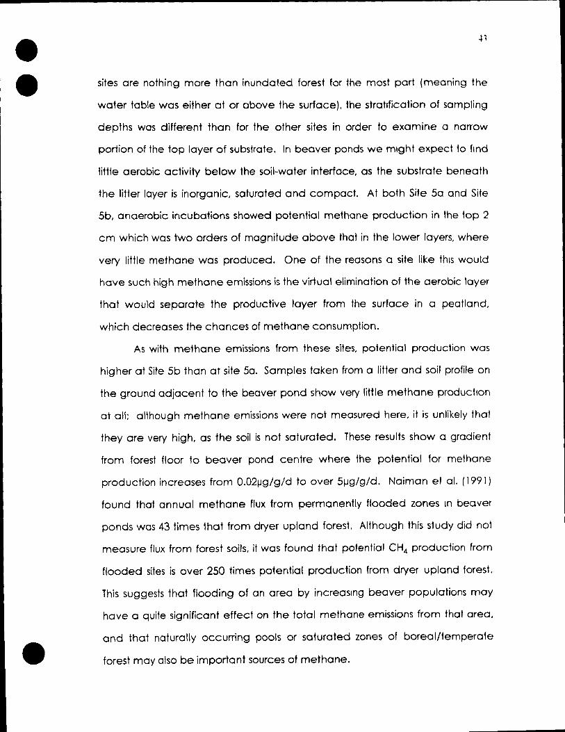
The results obtained trom incubations of profile samples at the Site 5 (the
beaver pond) show a different pattern than those of the peatlands. As these
• •
•
sites are nothing more than inundated forest for the most part (meaning the
water table was either at or above the surface), the stratification of sampling
depths was different thon for the other sites in order to examine a narrow
portion of the top layer of substrate. In beaver ponds we mlght expect 10 fmd
little aerobic activity below the soil-water interface, as the substrate beneath
the litter layer is inorganic, saturated and compact. At both Site Sa and Site
Sb, anaerobic incubations showed potential methane production in the top 2
cm which was two orders of magnitude above that in the lower layers, where
very little methane was produced. One of the reasons a site like thls would
have such high methane emissions is the virtual elimination of the aerobic layer
that would separate the productive layer from the surface in a peatland,
which decreases the chances of methane consumption.
As with methane emissions from these sites, potential production was
higher at Site Sb than at site 50. Samples taken from a lifter and soil profile on
the ground adjacent to the beaver pond show very little methane production
at ail; although methane emissions were not measured here, it is unlikely that
they are very high, as the soil is not saturated. These results show a gradient
from forest floor to beaver pond centre where the potential for methane
production increases from 0.02IJg/g/d to over 5I-Jg/g/d. Naiman el al. (1991)
found that annual methane flux from permanently flooded zones ln beaver
ponds was 43 times that from dryer upland forest. Although this study did not
measure flux trom forest soils, il was found that potential CH4 production from
flooded sites is over 250 times potential production from dryer upland forest.
This suggests that flooding of an area by increaslng beaver populations may
have a quite significant effect on the total methane emissions tram that area,
and that naturally occurring pools or saturated zones of boreal/temperate
forest may also be important sources of methane.
• •
•
It con be seen from figures 2.12 and 2.13 that methane consumption
under aerobic laboratory conditions is similor for most of the samples analyzed
(ranging from 0.52 to 3.75 I-/g/g/d), whereas methane production in anaerobic
incubations varies by nearly three orders of magnitude (ranging from 0.00 to
9.J2I-lg/g/d). Moore and Knowles (1990) found that consumption was greatest
between 0-50 cm, but that many peatland samples showed insignificant levels
of consumption under laboratory conditions. The highest rates of consumption
were found in samples from temperate swamps (170-250j.Jg/g/d), while
consumption in temperate bogs was in the range of 0-1 OOj.Jg/g/d in the top 50
cm. Bubier et al. (submitted) also found that consumption rates in peatland
inocula tended to be similar between sites and at a maximum near the water
table, but the range of values obtained in their study were quite different;
methane consumption rates ranged from 1-55I-lg/g/d, while production
spanned three orders of magnitude in the narrow range between 0-1I-lg/g/d.
Reasons for this difference in CH4 produdion/consumption potential are not
entirely cleor, but may be related to the different types of wetlands used in the
three studies .

• •
•
CHAPTER 3
This section of the thesis deals with one part of the problem of scaling
up methane emissions from wetlal1ds. The absence of a suitable inventory of
wetlands in a region makes it difficult to come up with accurate regional
estimates of CH4 emissions. It was 0150 discussed that spatial variability within
and between wetlands is great: the most accurate method of scaling up
methane emissions would take into account the typical methane emissions of
ecologically different wetland communities and their relative are a 1 coverage,
where data permitted. This chapter is concerned with the feasibility of using
remotely sensed data to classify ecologically different communities within
weflands, and will address several points:
• a comparison of the spectral changes in individual sites during the growing
season will be made.
• differences between sites will be considered in the context of how easily
these communities may be separated and classified using Landsat
imagery.
• changes in spectral reflectance as the field of view increases will be
examined to show how if hinders our ability to pick out individual species.
• comparisons of the "red edge" slope and values corresponding to bands of
Landsat imagery will be examined and compared between sites .

• •
•
46
study Area
The study was carried out on two fens in subarctic Quebec, Canada,
near the town of Schefferville (540 48'N, 660 49'W), an area charaderized by
hills and valleys running northwest to southeast, with a great deal of lakes.
Subarctic mires. such as the two considered in this study, are probably the
result of drainage interrupted by glaciation and the climatic effects of cold
winters and short moist summers. The Schefferville region is thought to coincide
with the centre of the northern Quebec/Labrador ice sheet, which retreated
about 6000 y BP. This has resulted in relatively young soils developed on a thin
layer of glacial drift which often shows similarities to the underlying bedrock.
Low nutrient content and pH are charac~eristic of soils underlain by quartzite or
shale. while those underlain by dolomitH typically have higher quantifies of
calcium and magnesium.
Wetlands in the study area are classified by the National Wetlands
Working Group (1988) as part of the low subardic peat land region. The
heterogeneous underlying geology, which comes from sediments of the
Labrador trough, results in spatially variable flora and subsurface water
chemistry (Moore et al 1990). Mineral rich fens are generally situated over
dolomite formations, whereas shales and quartzite are normally the substrates
of poor fens. These fens typically fall into one of several types, including open
fiat or patterned. minerai poor fens, surrounded by narrow margins of Larix
laricina, Picea mariana, Betula glandulosa, and other similar subarctic species.
Open fens oHen are charaderized by extensive, fiat sedge meadows, and the
centre of these fens is commonly flooded for part of the growing season, or
have small, shallow pools. The patterned fens often have a central pool and
ridge string complex. and lack any forested margin. Peat depths range trom 1-

• •
•
.. 7
2 m and although frozen for most of the year are not typically underlain by
permafrost.
The two fens studied, NASA fen and Astray fen {nomes are unofflcial).
had different charaderistics of vegetation and appearance. NASA fen was a
large open fen covered in sedges and grasses, with a flooded area, an area of
pools and strings, other small pools, moss hummocks, a foresfed margin, and a
few islands of torested margin type assemblages on raised sites. Astray fen was
large with several distinct communities, including a minerai poor area which
was very wef, a rich lawn section which sloped down to a small stream and
another rich treed area uphill trom the latter.
Concurrent with this study, research was done by others on methane
emissions trom the various plant communities in the two wetlands. Sites for
spectral analysis were chosen trom the sites used for methane emission
sampling, which were seleded on the basis of microtopography, hydrology
and vegetation (J. Bubier, pers. comm.). Over 25 small study plots were
seleded from different fen communities. These communities included string,
pool. sphagnum hummock, sphagnum lawn, sedge lawn and saturated areas
dominated by liverworts. Both poor and rich fen communities are represented,
incorporating bath wet and dry sites. A list of the sites used in this study, a brief
description of the site and the height trom which the spectral measurements
were taken are included in table 3.1. Tables 3.2 to 3.4 give the relative cover
of bryophytes and vascular plants in each study plot .

• •
•
Site Fen Height(m) Description
1 Astray 1 Pool 2 Astray 1 Hummock 3 Astray 1 Hummock/Pool 4 Astray 1 Hummock 5 Astray 1 Pool 6 Astray 1 Hummock 7 Astray 1 Hummock 8 Astray 0.15 & 1 Lawn 9 Astray 0.15 & 1 Lawn 10 Astray 0.15 & 1 Lawn 11 Astray 0.15 Hummock 12 Astray 1 PoolIHummock 13 Astray 1 Hummock 14 NASA 0.15 & 1 String 15 NASA 0.15 Hummock 16 NASA 0.15 Hummock 17 NASA 1 Pool 18 NASA 1 Lawn 19 NASA 0.15 & 1 Lawn 20 NASA 1 Pool
Table 3.1 Sites used for spectral reflectance measurement. the height at which they were measured and a brief description.

• •
•
Specles Site 1 Site 2 Sltf: 3 Site 4 SiteS Site 6 Sile 7 Sile 8 Site 9 Au/ocomlum Da/ustre 01 5 Cellleraon strammeum 01 01 01 CampvllUm stel/atum 01 01 01 1 Cmclldlum stvaum Cledopodlella (fU/tans 01 Dlcranum le/oneuron umrJnchfJa fflvo/vens LOBskvDnum badlum MY/la enomale Pelude/la sauarrosa 75 25 Plag,ommum e//IPfJcum 01 Poh/le nutans 01 POlytnchum stnctum 01 SeorDldlum seomodes 100 Sphaanum anausâfo/lum 50 5 Sphaanum annu/atum Sphaanum fuseum Sphaanum Imdbergl Sphaanum pulchrum SJlhagnum ruSSOWII 50 100 Sphaanum submtens Sphaanum tenerum Sphaanum wamstorfil 01 100 100 25 100 Tomenthvpnum mtens 100 01 01 01 Wernstorffa exennuletus 100
Specles Site 11 Site 12 Site 13 Sile 14 Site 15 Site 16 Sile 17 Site 18 Sile 19 Au/ocomlum palustre 01 01 CaUlergon stramtneum 01 CemDY/lum ste//atum 5 Cme/ldfum siYgum 01 C/edof)Odlella lJultans 100 Dlersnum /eloneuron 01 umpncht/a revo/vens 75 Loeskvtmum bedtum 20 MY/le anomale 5 1 Paludel/a sauarrose 1 1 Plagomnlum slllPt/eum Poh/la nutans Po/ytnchum stnctum ScolTJldtum scolTJlodes 25 Sphaonum anausbfollum 5 Spheonum annulelum 10 5 Spheonum fuscum 100 Spheonum hndbsrrll 80 95 Sphaonum Dulchrum 10 01 Sphaonum ruSSOWII Sphsonum submtens 20 Spheanum tenerum 100 5 Sphsanum wamstorlil 5 01 95 Tomenthypnum mtens 95 01 5 Wemstorffa s)(annulst~s 01 5
Table 3.2. Percent cover of bryophytes for sites ot which reflecfance was measured.
Site 10--
01
10
100
Site 20
100
01

• •
•
Specles 1 2 3 4 5 6 7 Andromeda gaucophylla 01 01 5 Aster radula 01 20 20 Betula riandulosa 10 2 ~,!Ia mlchauxlI Calamagrostls canadenSis 01 Carex._aqust/lls 01 Carex brunnescens 2 Carex cannescens 01
~!!!.!~X!Ji!._ Carex gynocrates 01 Carex mtenor Carex leDtalea Carex Iimosa 5 10 5 2 Carex Il v/da 20 Carex pauclflora Çarex paupercula Carex ranflora Çarex rostrata 30 Carex tenU/flora 5 Chamaedaphne cslyculata 20 ~PPtIS groenlandlca Drosera rotundlfolla 19'!!l!.etrum n/orum Emlob/Um anQust/tollum Ef]/Ioblum sp Habenana dllitata 01 Kalmla DoMolla 1 Lam<lancma 5 Ledum oroenlandlcum Lomcera villosa 2 Menyanthes tntollata 10 10 5 1 01 01 Mltella nuda Polvoanum vlVlparum 01 Potent/lla trut/coss 20 5 30 40 Pyrola asantolla Rubus acaulls 01 01 2 Sallx arctophl/a Sallx pedlcillans 01 Sa/ix vest/la SClrpus cesPifosus 5 2 Sc/fPUS hudson/anus 01 Se/af1lnella selaf1lnoldes 01 01 Smllacm.J Intol/a 2 10 SolldaQo ulll1nosa 01 10 10 Totie/dla puS/lia Tnaochm mant/ma 01 5 2 ~m/Um oxy.c0ccus 01 01
Table 3.3. Percent cover of vascular species for sites ot which reflectance was meosured (sites 1-10).
50
8 9 10
50 50 50
5
5 5 5
01
2

• •
•
51
Sp~cles 11 12 13 14 15 16 17 1I3-----r9 ---20 Andromedagaucophylla 01 2 01 As/er radula 01 8etu/a dandulosa 01 Betu/a m/chauxlI 5 5 CalamagrostJs canadensls 01 ----- -.--- .- - --~ -
Carex aQuatIJ/s 10 01 30 Carex brunnescens --r----- ------- -
Carex cannescens Carex eXIIIs 5 5 1 Carex ~nocrates 5 50
---1-----r- --- ------Carex mtenor Carex lepla/ea 5 --- f------
Carex ',mosa 1 01 20 5 10 10 20 Carex IIVlda Carex oauctffora 01 10 Carex oauoercu/a ----- r----.QJ ___ JO_ Carex fanf/ora - -- --
Carex rostrata 01 ---- --..-!Q -----~ 1 Carex tenu/trora
-.- - -- - --
Chamaedaphne ca/yculata 1 Coptls groenlandlca 5 Drosera rotundtfolla 01 01
r -- -- -- -- -
Em'petrum nl$1rum 2 01 ---- r- - -Epjob/Um arm.ustltollum ---- - ----
Eptlob/Um SI>. Habenana dllliala Kalmla oohfo/la 1 Lanxlancma 1 01 Ledum groan/andlcum 5
- -- -~- 1------
LOn/cera vII/osa 01 01 r-------Menyanthes tntollata 01 01 -20 20 5 Mltel/anuda 5 Polyganum vlvloarum ---- ----Patent/lia trot/casa Pyrola asanfol/a 01 ------------Rubus acaulls 2 10 Sal1x arctophlfa 10 5 Sai/x IJedlcll/ans Sa/ix vast/ta 10 SC/flJUS ceslJ/tosus 2 20 95 5 5 01
- -- ------SClfIJUS hudson/anus Se/aane/la selaanoldes 01 ---- ------- --Smlfacma tntolls 01 SO/Idago ullglnosa 1 1 1 01 Tofle/dla pUSIlis -- ------ --------Tnglochm mant/ma 30 Vaccmlum oxycoccus 01 01 01 .- --- -- - ---
Table 3.4. Percent cover of vascular species for sites ot which reflecfance wos measured (sites 11-20).

• •
•
52
Methods
Data was collected witl'l a Li-Cor 1800 spectroradiometer. The fi ber
optic attachment was fitted with a black PVC tube to give a field of view of
approximately 15°. Measurements of spectral reflectance were made
between 350 and 1100 nm in 1 nm increments; these were taken from heights
of 15 cm or 100 cm. depending on the field of view desired. Reference scans
were taken off a Kodak® grey cardo using the white side at a consistent
orientation and distance from the sensor; this information was used to convert
community reflectance data from mV to percent reflectance. This procedure
resulted in errors of less than 5% (for percent retlection) Nhen replicate
measurements were made on the reference panel.
Ali data collection was done under cloudless conditions between 1 Dam
and 4pm. local time. Sites were sampled in the same order on two dates. one
at the beginning of the growing season and one near the peak of the growing
season. In addition to spectral measurements. sorne plant semples were taken
to determine moisture content in the top 2 cm of the fen surface ot the time of
sompling.
Results and Discussion
Plots of percent reflectance vs wavelength for each of the 20 sites are
presented in appendix A. The sites used for this study were chosen as examples
of common vegetation communities. or in some cases to represent a single
species: for purposes of comparison and qualitative enalysis, variations
between sites and within site types will be considered. One of the problems
associated with wetland classification (and especially community

• •
•
differentiation within wetlands) is the issue of "mixed pixels". Sim ply stated, if our
sensor has a resolution of 10m, and the communities change on the order of
O.Sm, many of the 10m p:xels ma king up the scene will contain mixed spectral
information from a nurnber of communities. Such information may not be of
much use for classification, and to solve this problem we might need to use
higher resolution. To illustrate the point, measurement of the spectral properties
at some of the plots in this study was do ne at both 0.15m and 1 m. This increase
in measurement height changed the field of view trom approximately 0.015m2
to 0.3m2. Examination of the reflecfance plots for these ~ites should provide an
idea as to how changing resolution will alter the spectral response of a sample
plot.
Site 1 (Appendix A, Fig. AIl has only a minimal change in NIR (750 nm -
1100 nm) reflectance and virtually no change in visible reflectance over the
season. This is attributable to the fact that this site retains standing water over
the entire growing season, and has not enough vasculor plant coverage to
change its spectral characteristics. Sites 5, 17 and 20 (Appendix A, figs. A5, A21
and A24/ A251 are similor to site 1 in that they also maintain standing water, and
the same spectral pattern applies to each of them. Site 3 (Appendix Ar fig.
A3), which is a hummock surrounded by standing water, is also similor to site 1,
except that the difference in NIR later in the season is greater, due to the
drying of the hummock and growth of vascular plants.
" Site 2 (Appendix Ar fig. A2) is typical of hummocks in this study, as it ,Was
minimal variation in the visible portion of the spectrum, yet a significaJ1Y large
difference in NIR reflectance affer the second measurement. n~" pattern of ~
reflectance is not noticeably affected, but the reflectance itself is higher after
around 700 nm. Sites 7, 9(at lm), 11, 15 and 16 (Appendix.A, figs. A7, AIO, A14,
A 19 and A20) are other hummocks which follow the same pattern.

• •
•
54
Hummocks have similor reflectance patterns. but the magnitude of the
reflectance at any point in the spectrum may vary with dryness. moss species
and vascular plant development.
Site 4 (Appendix A. fig. A4) exhibits a tendency toward lower visible
reflectance and higher NIR reflectance later in the season. In addition to this
we con see more variation in the visible range, with a peak in the green region,
indicating the addition of new vegetation to the scene. Sites 6, 8(at 1 m) and
13 (Appendix A, figs. A6, AB and A 16) show similar patterns of reflectance
change over the sample period. Ali of these sites experience a drop in
reflectance in the red portion of the visible spectrum, perhaps due to an
increase in phofosynfhesis (thus chlorophyll) within the plants. Sites 12, 18 and
19 (Appendix A, figs. A 15, A22 and A23) are similar in pattern to these, except
they have higher reflectance in the visible and NIR range on the second
measurement.
Site 8 (Appendix A, fig. A8/A9) was a lawn site located in the rich lower
section of Astray fen, dominated by a bright green liverwort and including a
reddish green voriety of Sphagnum, with sedge growth increasing into the
growing season. The reflectance curve for measurements taken at 0.15m
shows an increase in reflectance across the specfrum over the 22 day sample
period. The plot for a sample height of 1 m is fairly different, as visible
reflectance decreases and NIR reflecfance increases over the sampling
period. Reflectance in the green and red visible range is slightly lower at 1 m,
but the temporal difference in NIR reflectance is pronounced. The effect of
the liverwort on the visible reflectance curve at 1 m is more defined in late July
thon it is at the beginning of the sampling period.
Sites 9 and 10 (Appendix A, figs. AlOI A 11 and A 12/ A 13) are both lawns
dominated by reddish green moss and include sorne carex cover. At site 9,

• •
•
the seasonal reflectance pattern at 0.15m is consistent and Increases across
the measured spectrum over the 22 day period. There is ::!ighfly more of an
increase in the red portion of the visible spedrum than in the green over time.
but it is quite minimal for both. As with site 8, NIR refledance shows a much
greater difference over time when sampled ot 1 m. At thls height. the
difference in visible refledonce ofter 22 days is negligible. Site 10 shows a
slightly different pattern. with NIR refledance decreasing and visible
refledance increasing over the period of measurement. Differences in the
reflectance peak are more pronounced from 0.15m, and NIR changes very
little when viewed trom 1 m. For 011 of these sites, the range of refledonce
values tends to be higher for measurements at 0.15m. Site 14 (Appendix A,
figs. A 17/ A 18), a string at NASA fen, exhibited very !ittle difference in
refledance across the spectrum, regardless of field of view.
When viewing a plot from O.15m, there is very little to get in the way of
refleded light and the sensor; in contrast, when we view from 1 m, vascular
plants ploya larger role in the refledance and scattering of light. Increasing
the field of view has the effed of smoothing the reflectance curve. essentially
a loss of some minor details aftributable to the spectral signature of certain
plants which may dominate the smc!ler scene. A comparison of refledance
between 630 and 690nm for sites measured at 0.15 and 1 m did not show any
relationship between the difference in reflectance at each height and percent
coyer of vascular plants. With a limited number of sites, this is most likely due to
the narrow range of differences in reflectance between the two heighfs.
Another example of loss of information is apparent in figure 3.1. This plot
shows the percent refledance of a string, a pool and string and pool both
occupying the field of view at the some time. In this case, the "mixed pixel"
exhibits the same pattern as the string, but there is an overall decrease ln
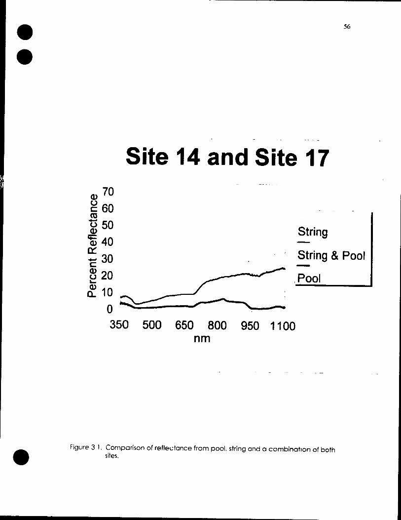
• •
•
56
Site 14 and Site 17
, String
String & Pool -,Pool
350 500 650 800 950 11 00 nm
Figure 3 1. Comparison of refledance from pool. string and a combinat.on of both sites.

• •
•
reflectance. This is especially true for the NIR portion of the spectrum, as the
increased moisture in the scene decreases reflectance in this range. Although
we would not be able to differentiate between string and pool for many pixels,
the average mixed pixel for such a community should be easily distinguished
from other communities wlTIlÎn the wetland, due to its characteristic spectral
properties.
Hummock and hollow topography is quite common in many North
American wetlands. Hummocks are raised mounds of moss. sometimes with
woody and herbaceous growth protruding trom the top. Hollows are
depressions in the wetland surface which are often found between hummocks
or in low-Iying areas of some lawn communities. Where local hydrology
permits, hollows may often resemble small pools and tend to have dork brown
or black vegetation growing at their bottom. As we can see from Fig. 3.2. the
two have very different spectral signatures. both in the visible and NIR regions
of the spectrum. At high enough resolution. it should be quite simple to obtain
relative coverage for each of these communities. which is almost imperative.
as they have quite different methane flux characteristics.
Sites 18. 19 and 20 are a series of plots which represent a graduai
change trom sedge/moss lawn to very shallow standing water. The spectral
refledance characteristics of these sites are shown in figure 3.3 for July 31. As
sites 18 and 19 have very similor vegetation. their spectral charaderistics are
very similar as weil. Site 20. on the other hand. with its standing water. shows
quite a different pattern of reflectance and is easily distinguishable trom the
other two.
It is cleor from figure 3.4 that different pools have ditferent spectral
reflectance characteristics. It seems that the distinguishing features become
more pronounced Icter in the growing season. and that the effect of the

• • 5R
Hummock and Pool 70
~ 60 c: .s 50 (.) Q)
~ 40 0:: C 30 Q)
~ 20 Q) c...
10
Hummock
Pool
o ~~--------~----~~~~-350 500 650 800 950 1100
nm
• Figure 3 2. Comparison of reflecfance from hummock and pool sites.

• •
Q) 70 g 60 co
Lawn and Pool
~ 50 Lawn (S18) 1E 40 ~ 30 Lawn (S19) c:: ~ 20 ~
~ 10 o 350 500 650 800 950 1100
nm
• Figure 3.3. Componson of reflectance from lawn and pool sites.

• • Cl> 20 o c ~ 15 Cl> ~
Cl> 10 œ: +-' c
Pools July 5
~ 5 ~ _____ a.. 0 i ~~_::.. ___ -----
","_, Site 1
Site 5
: Site 12
350 500 650 800 950 1100 nm
60
-- ------------------------
Cl> 20 0 c ~ 15 0 Q) ~
Q) 10 0:: -c
5 Cl> 0 ..... Q) a.. 0,
350
Pools July 27
~--~~-----~
Site 1
. Site 5
~ Site 12
500 650 800 950 1100 nm
• Figure 3.4. Comparison of reflectance trom various pool sites.

• •
•
presence of vascular plants is quite significant. For example, site 12, whlch has
the highest reflectance, the only visible green peak and the most variation of
the three sites also has the highest incidence of vascular plants. The
appearance of such features in this figure are quite striking, but when it is
considered that the reflectance is below 20% for the entire measured
spedrum, there can be little doubt that such communities would still be easily
distinguished from hummocks or lawns.
The common reflectonce properties of vegetation as described in
Chapter 1 proved to be shored by most of the plots sam pied in this study.
Pools and wet hollows or lawns were different, and usually had fairly low
reflectance across the spectrum of measurement, due to the low density of
green vegetation in those scenes. With only 3 exceptions (sites 10, II and 15),
NIR refledance was always greater on the sampling date later in the season,
perhaps because water levels had dropped sufficiently at most sites. resulting
in less NIR absorption.
As water content in a plant is related to the amount of NIR absorbed or
reflected, it seems Iikely that moisture content in the top 2 cm of the peat
should be related inversely to measured NIR. Such a relationship was found to
be very weak. The spectroradiometer is "seeing" vascular plants and
bryophytes, but we are only measuring moisture in the bryophytes, so the
efficiency of our relotionship is bound to be reduced. The relotionship between
percent cover of vascular species and NIR reflectance was olso weok,
indicating that the interaction of factors offecting NIR refledance is more
complex than a simple linear relationship. Qualitotively, if we compare pools,
strings, lowns and hummocks, the relationship is actually quite obvious, with the
drier sites having higher NIR reflectance .

• •
•
62
One way in which pools. lawns and hummocks may be distinguished is
by examination of the slope of percent reflectance in an area of the spectrum
known as the red edge, which spans trom 680 nm to 750 nm. This is the region
where the typically low reflectance in the visible spectrum gives way to high
reflectance in the NIR, and the communities differ in this respect. Pools in this
study have a mean slope of 2.3 and standard deviation of 0.3, lawns have a
mean slope of 4.4 and standard deviation of 0.9, and hummocks have a
mean red edge slope of 8.7 with a standard deviation of 2.0. Vogelmann and
Moss (1990) attribute steeper red edge si opes to high chlorophyll content in
Sphagnum. although in this case it probably has more to do with increased
vegetation density as we progress trom pools to hummocks.
Mean values of percent reflectance for wavelengths corresponding to
various Landsat TM and MSS bands are presented in figures 3.5 to 3.7. From
these figures one con see that the different communities (Iawn, hummock and
pool) are separated by their distinctive characteristics in some cases,
especially MSS band 5 and TM band 3. This indicates that several wavebands
of Landsat sensors are suitable for differentiating between the communities, but
it is not certain that the relatively coarse resolution would be able to separate
communities with similar spectral properties but different characteristic values
of methane flux.
If one knows the percent reflectance and mean seasonal methane flux
of individual communities, as weil as- how much area each community
occupies in a typical larger site, the percent reflectance and mean seasonal
methane flux of the larger site can also be estimated. If these compare
successfully with the remotely sensed image, then an estimate of mean
seasonal methane flux trom the wetland con be obtained, provided the
appropriate data is available for 011 communities within the wetland. Allow 2

•
•
.-.50 Q) 0
ffi 40 tS Q)
iii 30 '-
~ 0
'-'20 v
Percent Reflectance of 1 m plots
1 ~
1
p
I? p
p
h h
h h~
2 4 6 8 tm band 3 (0/0 reflectance)
Figure 3.5. Percent refledance in the range of Landsat TM band 3 and 4 for plots measured from one metre (p=pool. h=hummocl<. 1=lawn).
10
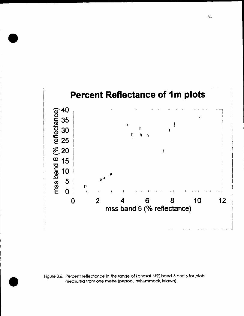
•
•
Percent Reflectance of 1 m plots
â)40 0 c 35 «J .... ~ 30 ~ 25 ~ 20 \ ---«) 15 "C
~ 10 oC en 5 en E 0 1
o
p
h h
h h h
p pP
1- - ,- - - \ - j 1- - - t
2 4 6 8 10 mss band 5 (% reflectance)
1
1
- 4 - ~--J 12
1
___________________ J
Figure 3.6. Percent reflectance in the range of landsat MSS band 5 and 6 for plots measured from one metre Ip=pool. h=hummocl<, 1=lawn).

•
•
Percent Reflectance of 1 m plots
0)50 o r c: f
~ 40 1
(1) Q::
~ 30 J '#. ........"
...... 20 't:S c: ~ 10 U) U) p E 0 +- -+
o
p
p - 1-
p
h h h h
h
2 4 6 8 10 mss band 5 (0/0 reflectance)
Figure 3.7. Percent reflectance in the range of Landsat MSS band 5 and 7 for plots measured from one metre (p=pool, h=hummock, 1=lawn).
12

• •
•
66
larger sites trom NASA fen be used as an example of where this process may
fail using coarse resolution data. A very wet site consisting of about 90%
standing water (site 20) and 10% sedge lawn (site 18) has a weighted mean
seasonal CH4 flux of 42 mg/m2/d and a weighted MSS band 5 refledance of
3.5%. A patterned site with coverage of approximately 35% strings and 65%
pools has a weighted mean seasonal CH4 flux of 19 mg/m2/d and a weighted
MSS band 5 refledance of 5%. Although the CH4 flux is more than twice as
high ot the first site, the difference in MSS band 5 reflectance is negligible.
Landsat images of NASA fen showed Httle difference in DN values for
these sites. The pixels which represent these sites in the satellite image are an
average of refledance data from several communities, which in many cases is
a simple loss of information. This point is further illustrated if we consider sites
such as 3, 12 and 19 (which represent the equivalent of mixed pixels). The
percent reflectance of these sites, wh en averaged over the previously
discussed Landsat bandwidths, places them between community groupings or
in a potentially misleading community grouping. Site 3 is a moss hummock
surrounded by water on ail sides, but mean percent reflecfance in MSS band 5
would indicate that it is a pool. Site 12 is the opposite, a small pool surrounded
by mosses and vascular plants, and fits between hummock and pool
categories in MSS band 5. Site 19 is a lawn community which is as wet as a site
cou Id be without having standing water; ifs MSS band 5 refledance is situated
between pools and hummocks .

• •
•
SUMMARY AND CONCLUSIONS
Methane flux averaged over H'e season in the Eastern lemperate Boreal
Region ranged from 0.18 to 1071 mg/m2/d at 5 sites dunng the frost-free penod
of 1991. Bog sites, as in many other studies, exhibited quite low methane flux.
ranging trom 0.18-3.40 mg/m2/d at sites 1 a to 1 c. Moderate values of
methane flux for this study were found at site 1 d. 2 and 3 (wet bog, swomp and
shore bog), which had seasonal mean flux values of 70, 50 and 99 mg/rn"/d,
respectively. The largest values of seasonal mean CH 4 flux were meosured at
sites 4 (floating mat) and 5a/5b (beaver pond edge/centre) to be 1071. 396
and 694 mg/m2/d, respectively. These values were generally in agreement
with other studies of similor wetlands, with the exception of site 5 (which
exhibited larger CH4 flux thon previously measured beaver ponds) and sites 3
and 4, of which there were no comparable studies ln the literature. ft would be
useful to establish the areal extent of wetlands such as sites 3 and 4, m the
seasonal mean flux from these wetlands is sufficiently high to make them a
significant contributor to regional methane emissions.
Sites whlch exhibited the highest flux always had a relatlvely high
seasonal water table position, and a relationship was found to exist between
log mean seasonal methane flux and mean seasonal water table position at
peatland sites (1 a-d and 2); statistics derived from the regression of thls
relationship were within the range of those determined by Moore and Roulet
(Geophysical Research Papers, in press) for many other North American
peatlands. Relationships between CH4 flux and temperature were less
common, and only in some instances did temperature signifJcantly help to
explain seasonal flux patterns. It is possible that befter flux-temperature
•
•
68
relafionships would have been evident if sail temperature measurements at the
beaver pond site had been made on a regular basis.
Episodic fluxes have been found ta make up a significant part of the
seasonal emissions for the peatlands in this study. Had measurement of these
events been missed during the sampling season, estimates of mean seasonal
emissions would have been underestimated by up ta 160%, and site 1 a would
have qualified as a net consumer of methane. Although sampling on a 10-15
day interval may give accurate estima tes of the regular seasonal flux pattern,
episodic fluxes require a smaller sampling interval, and have proven to be an
important component of seasonal emissions.
ln order to explain the patterns of seasonal methane flux, it is necessary
to look at more than just the environmental variables. Incubation of peat
samples from our study provide valuable information regarding the
expia nation of methane emission magnitude and seasonal patterns. There still
remc..'ln some cases where measurement of these variables cou pied with
simple incubations are insufficient to explain the magnitude and/or CH4 flux
magnitude at sorne sites. Methane production in the laboratory may be a
fairly good indicator of what to expect in the fi~ld, but in some cases a large
production potential does not mean large seasonal emission values, and vice
versa.
Incubation of samples trom a beaver pond showed that CH4 production
is highest in the top 2 cm of substrate. If has been shown here that there is a
gradient of increasing CH4 production potential and flux as we go from forest
tloor to beaver pond centre. This indicates that the shallow flooding of
forested land has the effect of increasing the substrate's ability to produce
methane. Increases in beaver population or forest flooding by other means
may increase regional methane emissions.

•
•
What separates wetlands from the surrounding landscape spectrally IS
their wetness. which manifests itself in NIR contrast between wetland. forest and
soil. This contrast should be greatest in spring, after the snow has gone but
before water levels drop tao far below the surface. indicating that wetland
classification using remote sensing is besl done at this time. Reflectance ln the
visible portion of the spedrum and NIR refledance in waterlogged
communities appears to change very IiHle over the growing period. NIR
refledance is generally greater and vascular plants (which may help to
spedrally charaderize a community) are likely to be developed later ln the
growing season; this would suggest that infra-wetland variabilily in comrnunity
spedral characteristics may have greater contrast as we approach Ihe fall. Il
is likely. however. that such differences are great enough even at the
beginning of the growing season to differentiate the various communities.
Methane flux measurements in this study suffered trom large spalial and
temporal variability. which hindered interpretation la sorne extenl and
diminished the usefulness of the data. In future studies, thls could be
overcome by dividing sites into sub-sites with similor microtopography and
water table charaderistics. as weil as la king more measurements on each
sampling date to decrease errors. Water table and soil tei'nperature should be
monitored more closely ta betfer undersland the relationships between these
variables and methane flux.
The next logical step in Ihis approach 10 scaling up methane ernl~sions 15
ta integrate a study of methane flux from wetlands in a given region with a
small scale remote sensing projed to complement the flux sites. A prelimlnary
study to determine the major wetland tvpes in the reglon would be useful. as
would finding representative and accessible examples of these wetlands 10 be
used in the sludy. Such a projed should include a clear definition of welland

• •
•
70
communities whlch are important in terms of methane flux at the beginning of
the pro/ect. This would allow the flux data to be easily linked with ground truth
data acqulred by means of a spectroradiometer.
It would be benefÎCIal to use a spedroradiometer with a broader
spectral range than the one used in this study, in order to simulate more
Landsat bands and to get information from thermal IR wavelengths. If possible,
airborne sensors could be set up to measure reflectance in wavebands which
are best at distinguishing between communities. This would serve the dual
purpose of provlding both valuable spectral information and increasing the
resolutlon at which the data are collected, which would help solve the
problems assoclated wlth mixed pixels encountered in this study .

•
•
lITERATURE ClTED
Aaby, B. and Berglund, B.E. 1986. Charaderization of peat and loke deposiis.
ln the Handbook of Holocene Palaeoecology and
Palaeohydrology. B.E. Berglund. ed.. John Wiley and Sons, New
York.
Aselmann, 1. and Crutzen, P.J. 1989. Global distribution of natural freshwater
wetlands and rice paddies, their net plirnary productivlly,
seasonality and possible methane emissions. Journal of
Atmospheric Chemistry 8:307-358.
Berglund, B.E. (ed.) 1986. Handbook of Holocene Palaeoecology and
Palaeohydrology, John Wiley and Sons, New York.
Bridgham, S.D. and Richardson, C.J. 1992. Mechanisms controlling soil
respiration (C02 and CH4) in southern peallands. Soil Biology and
Biochemistry 24: 1 089-1 099.
Bubier, J.l., Moore, T.R. and Roule!, N.T. Submilled. Methane emissions trom
wetlands in the boreal region of Northern Ontario, Canada.
Ecology.
Cicerone, R.J. and Oremland, R.S. 1988. Biogeochemical aspects of
otmospheric methane. Global Biogeochemical Cycles 2:299-327.
Dunfield, P., Knowles, R., Dumont. R. and Moore, T.R., ln pres!:.. Methane
production and consumption in temperate and subardic peat
soils: response to temperature and pH. Soil Biology and
Biochemistry .
Ford, T.E. and Naiman, R.J. 1988. Alteration of carbon cycling by beaver:
methane evasion rates from boreal forest streams and rivers.
Canadian Journal of Zoology 66:529-533 .

•
•
Fung, 1., John, J., Lerner, J., Matthews, E., Prather, M., Sfeele, L.P. and Fraser, P.J .
1991. Three-dimensional model synthesis of the global methane
cycle. Journal of Geophysical Research 96: 13,033-13,065.
Gausman, H.W. 1985. Plant leaf optical properties in visible and near-infrared
light. Graduate Studies (Texas Tech University) No. 29. Texas Tech
Press, Lubbock, Texas.
Government of Quebec 1989. Peatlands and remote sensing: Inventory of
peatlands in Northern Quebec. Quebec Ministry of Energy and
Resources.
Grant, L. 1987. Diffuse and specular characteristics of leaf reflectance.
Remote Sensing of Environment 22:309-322.
Harriss, R.C., Gorham, E., Sebacher, D.I., Bartlett, K.B. and Flebbe, P.A. 1985.
Methane flux from northern peatlands. Nature 315:652-654.
Khalil, M.A.K. and Rasmussen, R.A. 1990. Constraints on the global sources of
methane and an analysis of recent budgets. Tellus 42B:229-236.
Matthews, E. and Fung, 1. 1987. Methane emission from natural weflands:
global distribution, area, and environmental characteristics of
sources. Global Biogeochemical Cycles 1 :61-86.
Moore, T.R. 1988. Atmospheric methane. The Canadian Geographer 32: 178-
184.
Moore, T.R. and Knowles, R. 1990. Methane emissions from fen, bog and
swamp peatlands in Quebec. Biogeochemistry 11 :45-61.
Moore, T.R. and Roulet, N.T. 1991. A comparison of dynamic and static
chambers for methane emission measuremenfs from subarctic
fens. Afmosphere-Ocean 29:102-109 .

•
•
Moore, T.R. and Roulet, N.T. In press. Methane flux:water table relations in
northern wetlands. Geophysical Research Letters.
Moore, T.R., Roulet, N.T. and Knowles, R. 1990. Spatial and temporal variations
of methane flux from subardic/northern boreal fens. Global
Biogeochemical Cycles 4:29-46.
Naiman, R.J., Manning, T. and Johnston, C.A. 1991. Beaver population
fluctuation~ and tropospheric methane emisslon in bore a 1
wetlands. Biogeochemistry 12: 1-15.
National Wetlands Working Group 1988. Wetlands of Canada. Ecological
Land Classification Series NO.24. Sustainable Development
Branch, Environment Canada, Ottawa, and Polyscience
Publications, Montreal.
Ramanathan, V., Cicerone, R.J., Singh, H.B. and Kiehl, J.T. 1985. Trace gas
trends and their potential role in climate change. Journal of
Geophysical Research 90:5547 ~5566.
Ramanathan, V. 1988. The greenhouse theory of climate change: a test by an
inadvertent global experiment. Science 240:293-299.
Rodhe, H. 1990. A comparison of the contribution of various gases to the
greenhouse effect. Science 248:1217-1219.
Roulet, N.T., Ash, R. and Moore, T.R. 1992. Low boreal wetlands as a source of
atmospheric methane. Journal of Geophysical Research 97:3739-
3749.
Schmid, H.P. and Oke, T.R. 1990. A model to estimate the souce area
contributing to turbulent exchange in the surface layer over
patchy terrain. Quarterly Journal of the Royal Meteorological
Society 116:965-988 .

•
•
Sebacher, 0.1., Hmnss, R.C., Bartlett, K.B., Sebacher, S.B. and Grice, S.S. 1986 .
Atmospheric methane sources: Alaskan tundra bogs, an alpine
fen and a subarctic boreal marsh. Tellus 38B: 1-1 O.
Singhroy, V. and Bruce, B. 1979. Wetlands mapping in Northern Manitoba-an
application of enhanced Landsat data. Canadian Centre for
Remote Sensing paper # 1 04061 O.
steele, L.P., Fraser, P.J., Rasmussen, R.A., Khalil, M.A.K., Conway, T.J., Crawford,
A.J., Gammon, R.H., Masarie, K.A. and Thoning, K.W. 1987. The
global distribution of methane in the troposphere. Journal of
Atmospheric Chemistry 5:125-171.
Steele, L.P., Dlugokencky, E., Lang, P.M., Tans, P.P., Martin, R.C. and Masarie,
K.A. 1992. Siowing down of the global accumulation of
afmospheric methane during the 1980s. Nature 358:313-316.
Svensson, B.H. and Rosswall, T. 1984. In situ methane production from acid
peat in plant communities with different moisture regimes in a
subarctic mire. Oikos 43:341-350.
Tomlins, G.F. and Thomson, K.P.B. Toward an Operational, Satellite-Based,
Wetland Monitoring Program for the Fraser River Estuary, British
Columbia. In Proceedings of the Seventh Canadian Symposium
on Remote Sensing, Winnipeg, Manitoba.
Troels-Smith, J. 1955. Characterization of unconsolidated sediments. Danm.
Geol. Unders. IV 3: 1-73.
Vogelmann, J.E. and Moss, D.M. 1992. Spectral analyses in the genus
Sphagnum using Landsat TM and high spectral resolution
laboratory measurements. International Geoscience and Remote
Sensing Symposium paper, IEEE Catalog No. 92CH3041-1, Library of
Congress No. 91-72810 .

•
•
Walter-Shea, E.A. and Biehl, L.L. 1990. Measuring vegetation spectral
properties. Remote Sensing Reviews 5: 179-205.
Wang, W.C., Wuebles, D.J .. Washington. W.M .. Isaaes, R.G. and Molnar. G.
1986. Trace gases and other potential perturbations to global
climate. Reviews of Geophysics 24: 11 0-140.
Weyhenmeyer, C.E. 1992. Methane emissions from a boreal beaver pond.
Masters thesis, Watershed Ecosystems Graduate Program. Trent
University, Peterborough, Ontario, Canada.
Whalen, S.C. and Reeburgh, W.S. 1990. Consumption of atmospherie
methane by tundra soils. Nature 346: 160-162.
Wilkinson, L. 1990. SYGRAPH: The system for graphies. Systat, Inc., Evanston, IL.
Williams, R.T. and Crawford, R.L. 1985. Methanogenic baderia, inclucJing an
acid-tolerar,t c;train, from peatlands. Applied and Envlronmental
Microbiology 50: 1542-1544.
Windsor, J., Moore, T.R. and Roulet, N.T. 1992. Episodic fluxes of methane from
subardie fens. Canadian Journal of Soil Science 72:441-452.
Woolley, J. T. 1971. Reflectanee and transmittance of light by leaves. Plant
Physiology 47:656-662.
Zoltai, S.C. and Pollett 1983. Wetlands in Canada: their classification,
distribution and use. In: Gore, A.J.P. (Ed.), Ecosystems of the world
4B Mires: swamp, bog, fen and moor. Elsevier, Amsterdam, The
Netherlands .

• TABLE OF CONTENTS
Page
Abstract
Résumé ii
Acknowledgments iii
lis t of tables and figures iv
Chapter 1: Foreword and introduction 1 - specifie objectives 1 - introduction 2
Chapter 2: Methane emi!.sions from the Eastern Temperate Wetland Region 13 - site descriptions 13 - methods 15 - results and discussion 19 - incubation of soil samples 35
Chapter 3: Spectral characteristics of subarctic fens 45 - study area 46 - methods 52 - results and discussion 52
Summary and Conclusions 67
literature Cited
Appendix A: Percent reflectanc(~ of subarctic fen site!.
Appendix B: Mean daily methcne flux for Eastern Temperate wetland sites
•

• •
•
APPENDIX A
Percent reflectance for 011 sites on both sampling dates .

• •
cu 70 g 60 ca t5 50 cu
Site 1 (1m)
~ 40 July 5th 0:::
C 30 Jul 27th ~ 20 L...
~ 10
o 350 500 650 800 950 11 00
nm
• Figure A 1 Percent reflectance at site l, measured from lm.

• •
70
~ 60 c .s 50 o ~ 40 Q)
0:: 30 ..... c: ~ 20 '-
~ 10
o
Site 2 (1m)
July 5th
. Jul 27th
350 500 650 800 950 11 00 nm
• Figure A2 Percent reflectance ot site 2, measured trom 1 m,

• •
Q) 70 g 60 ro (350 Q)
~40 c::: "E 30 ~ 20 .... ~ 10
o
Site 3 (1m)
July 5th
'Jul 27th
350 500 650 800 950 11 00 nm
• Figure A3 Percent reflectonce ot site 3. measured trom 1 m.

• 1.
Cl) 70 g 60 co ~ 50 ~ 40 a::: -+-' 30 c: ~ 20 L.-
~ 10 o
Site 4 (1m)
350 500 650 800 950 1100 nm
• Figure A4 Percent reflectance at site 4. measured from 1 m
July 5th
Jul 27th

• •
Q) 70 g 60 ro U 50 Q)
~ 40 c:: ...., 30 c: ~ 20 '-
~ 10 o
Site 5 (1m)
~-----------------~----.# 350 500 650 800 950 11 00
nm
• Figure A5 Percent reflectance ot site 5, meosured from lm.
July 5th
Jul 27th

• •
Q) 70 g 60 ca ~ 50 '$ 40 0::: ..... 30 c: ~ 20 '-
~ 10 o
Site 6 (1m)
350 500 650 800 950 11 00 nm
• Figure A6 Percent reflectance at site 6. measured trom 1 m
July 5th
Jul 27th

• •
ID 70 g 60 ro ~ 50 ~ 40 0:: ..... 30 c: ~ 20 '-
~ 10 a
Site 7 (1m)
350 500 650 800 950 1100 nm
• Figure A7 Percent reflectonce ot site 7. measured fram 1 m
July 5th
Jul 27th

• •
70 ID g 60 cu t5 50 ID
~40 0::: C 30 ~ 20 ~
~ 10
o
Site 8 (1m)
350 500 650 800 950 1100 nm
• Figure A8 Percent reflectance at site 8. measured from 1 m.
July 5th
Jul 27th

• •
70 Cl)
g 60 ctS t5 50 Cl)
ID 40 0::: E 30 820 ~
~ 10
o
Site 8 (O.15m)
350 500 650 800 950 1100 nm
• Figure A9 Percent reflecfance at site 8. rneasured fram 0 15 rn.
July 5th
Jul 27th
i
_J

-~-----------------
• •
Site 9 (1m)
70 Q)
g 60 co t5 50 Q)
~ 40 ~ C 30 ~ 20 '-
~ 10
o 350 500 650 800
nm 950 1100
• FI~lurt:' Al 0 Percent refleclance al site 9. measured from lm
July 5th
Jul 27th

• •
70 Q)
g 60 ro
1:5 50 ID
'ID 40 0:: -- 30 c: ~ 20 L..
~ 10
0 350
Site 9 (O.15m)
500 650 800 950 nm
• Figure A 11 Percent reflectance ot site 9. measured tram 015 m
....
July 5th
Jul 27th
1100
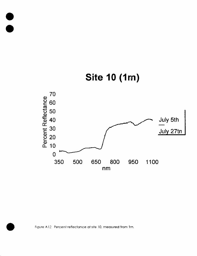
-----------------------
• •
70 Q)
g 60 co U 50 Q)
1fi 40 ~ "E 30 ~ 20 L-
~ 10
o
Site 10 (1nn)
.r-'" July 5th
Jul 27tn
350 500 650 800 950 1100 nm
• Figure A l ~ Percent reflecfonce ot site 10. meosured from 1 m.

• •
70 (l)
g 60 co
1:5 50 (l)
(ü 40 c::: C 30 ~ 20 '-
~ 10
o
Site 10 (O.15m)
350 500 650 800 950 1100 nm
• Figure A 13. Percent reflectance at site 10. measured fram 0 15 m
July 5th
Jul 27th

• •
(J) 70 g 60 cu t5 50 (J)
Site 11 (O.15m)
iD 40 0::
, July 5th
C 30 ~ 20
Jul 27th .... ~ 10
o 350 500 650 800 950 1100
nm
• Figure A 14 Percent reflectonce ot site 11, measured fram 0.15 m.

• •
Q) 70 g 60 co t) 50 Q)
~ 40 0::: C 30 ~ 20 ~
~ 10 o
Site 12 (1m)
350 500 650 800 950 1100 nm
• Figure A 15 Percent reflectance ot site 12, measured fram 1 m
July 5th
Jul 27th

• •
ru 70 g 60 cu t5 50 ru 't 40 a:: C 30 ~ 20 '-
~ 10 o
Site 13 (1m)
350 500 650 800 950 1100 nm
• Figure Al b Percent reflectance at site 13. measured tram 1 m.
July 5th
Jul 27th

• •
ID 70 g 60 co t5 50 ID
1i3 40 cr: C 30 ~ 20 '-
~ 10 o
Site 14 (1m)
350 500 650 800 950 1100 nm
• Figure A 1 7 Percent reflectonce ot site 14, measured trom 1 m
July 4
Jul 31

• •
ID 70 g 60 co t5 50 ID
ID 40 a: C 30 ~ 20 '-
~ 10 o
Site 14 (O.15m)
350 500 650 800 950 1100 nm
• FI~urt::) A 18 Percent reflectonce at site 14, measured From 0 15 m
July 4
Jul 31

• •
ID 70 g 60 co U 50 ID
1G 40 0:: C 30 ~ 20 ~
8: 10 o 350
Site 15 (O.15m)
500 650 800 950 1100 nm
• Figure A 19 Percent reflec tancE:' ot site 15 rnE:'murf~d frürn 0 l'sm
July 4
Jul 31

• •
Q) 70 g 60 co t5 50 Q)
~ 40 ~ 'E 30 ~ 20 ~
~ 10 o
Site ~16 (O.15m)
350 500 650 800 950 11 00 nm
• Floure A~O Percent refleclonce of sile 16. meosured from 0 15 m.
July 4
Jul 31

• •
Q) 70 g 60 ca ts 50 Q)
~ 40 0:: ~ 30 c: ~ 20 ~
~ 10 o
Site 17 (1m)
--~-------~------~/ ,--------.., 350 500 650 800 950 1100
nm
• Figure A21. Percent reflectance ot site 17. measured from 1 m
July 4
Jul 31

• •
Q) 70 g 60 co ts 50 Q)
15 40 0:: C 30 ~ 20 .... ~ 10
o 350
Site 18 (1m)
500 650 800 nm
,July 4
Jul 31 ----"'_ ....
950 1100
• Figure A~2 Percent reflecfance ot site 18, measured from 1 m.

• •
cu 70 g 60 ca ....., u 50 cu ~40 ~ E 30 ~ 20 ~
~ 10
a
Site 19 (1m)
3EiO 500 650 800 950 1100 nm
• Figure A23. Percent reflectance at site 19. measuied from lm
July 4
Jul 31

• •
Q) 70 g 60 co t5 50 Q)
1E 40 ~ E 30 ~ 20 ~ 10
o
Site 20 (1m)
350 500 650 800 950 1100 nm
• Figure A~4 Percent reflectonce ot site 20, measured from 1 m.
July4

(1) 70 g 60 ro t) 50 (1)
~ 40 c:: E 30 ~ 20 '-
~ 10 o
Site 20 (O.15m)
350 500 650 800 950 1100 nm
• Figure A25. Percent reflectonce ot site 20. measured trom 0 15 m
July4

• •
•
APPENDIX B
Mean daily methane flux for 011 sites over the sampling season .

• •
•
Date Julian Day Site la Site 1 b Site le Site Id
May 13 133 0.3 2.8 5.5 1.3 May 20 140 -0.6 3.7 4.9 4.2 May 27 147 0.5 -0.7 1.8 7.7 June 10 161 0.4 6.1 0.6 89.9 June 17 168 -0.9 0.0 -0.9 88.9 June 24 175 -0.1 2.8 0.1 36.2 June 29 180 0.1 0.1 0.0 155.2 July 8 189 0.6 0.7 -0.2 47.1 July 13 194 0.5 1.9 0.0 232.7 July 22 203 -0.4 2.6 -1.3 259.7 July 29 210 4.4 39.9 6.4 181.9 August 5 217 0.1 -0.7 -0.3 42.7 August 12 225 -0.3 3.8 0.1 134.2 August 19 232 -0.2 -0.3 -1.0 51.7 August 26 239 -0.2 0.4 -0.5 0.1 September 1 4 258 -0.1 -0.1 -0.1 5.7 Oetober 2 276 -0.6 -0.2 -0.2 2.7 Oetober 18 292 0.1 -0.1 -0.1 0.9 November 2 307 -0.3 -0.3 -0.2 0.4
Figure B 1. Meon doily methone flux (mg/mL Id) ot sites 10 - 1 d over the ~ompling season.

• •
•
Date Julian Day Site 2 Site 3 Site 4 Site 50 Site 5b
May 14 134 2.4 119.5 643.8 22.2 May21 141 1.6 226.5 23.0 4.7 May 28 148 15.1 458.9 86.5 27.9 June 11 162 35.3 17.1 543.6 179.4 June 18 169 45.7 62.5 499.9 74.1 June 25 176 27.2 188.7 411.5 525.4 July 2 183 108.1 2890.9 172.9 444.2 July 9 190 15.9 645.3 112.9 816.4 July 14 195 16.8 76.9 1883.7 430.3 929.3 July 23 204 43.2 13.8 2080.9 427.8 815.4 July 30 211 277.0 53.2 1445.1 504.2 644.3 August 6 218 34.3 113.9 1860.7 1141.7 400.2 August 13 226 129.5 66.2 256.3 952.0 722.9 August 20 233 63.6 140.1 1489.0 761.4 1254.9 August 27 240 79.3 118.3 1359.3 583.2 547.0 September 8 252 10.4 18.7 641.6 948.9 679.0 September 20 264 46.3 7.7 2927.0 495.2 516.9 Ocfober 6 280 6.5 13.2 642.5 11 1.2 1013.0 October 20 294 1.5 1.9 25.8 85.0 239.1 nov 9 314 377.1
Figure B~. Mean daily methane flux (mg/m2/d) af sites 2 - 5b over the sampling season