westfälische wilhelms-universität münster volkswirtschaftliche diskussionsbeiträge ·...
TRANSCRIPT

Westfälische Wilhelms-Universität Münster
Volkswirtschaftliche Diskussionsbeiträge
Beitrag Nr. 324
Trond-Arne BorgersenAgder University College
Postuttak / 4604 Kristiansand / Norway
Matthias GöckeWestfälische Wilhelms-Universität Münster /
Institut für Industriewirtschaftlische Forschung
Universitätsstraße 14-16 / D-48143 Münster / Germany
www.Matthias-Goecke.de
Kristiansand and Münster, August 2001
Preliminary draft! Work in progress!Please contact authors for the latest version!
Overshooting and Hysteresis
by Trond-Arne Borgersen
and Matthias Göcke
Overshooting and Hysteresis
by Trond Arne Borgersen and Matthias Göcke
Abstract:* This paper integrates a traditional Dornbusch overshooting model with a macro-
economic model of hysteresis in foreign trade. The concept of hysteresis in the model is
represented via an aggregation approach that is equivalent to the original concept of hysteresis
in magnetics with a continuous hysteresis-loop. This combined framework shows how a
situation with sticky prices and short run exchange rate overshooting results in long run
persistence in exchange rates. Monetary shocks can lead to hysteresis in both foreign trade and
exchange rate processes, invalidating the long run neutrality of money hypothesis of the
conventional overshooting model.
JEL-Classification: E12, F31, F41
Keywords: exchange rates, Dornbusch model, hysteresis, foreign trade, PPP
1. Introduction
The seminal overshooting model of Dornbusch (1976) has been the key reference regarding
the long run neutrality of money for the last twenty-five years. Monetary shocks are assumed
to affect real variables in the short run while prices are sticky, but as prices adjust are the
shocks neutralised, and the real effects decay over time.
The economic turbulence of the 80s, with large exchange rate misalignments questioned the
validity of the long neutrality hypothesis. Several authors claimed that economic systems
could contain hysteresis, making economic processes path dependent and to some extent
invalidating the reasoning based on unique long run equilibrium (e.g. Layard et al, 1991, or
Soskice et al, 1989). The hysteresis approach at first gained strength within labour market
theories (Lindbeck, Snower, 1988, or Gottfries, Horn, 1987), but after some time it was
introduced to economics in general. The relationship between foreign trade and exchange
rates was one of the new extensions of the theory.1 Baldwin (1989), Baldwin, Krugman
(1989) and Dixit (1989, 1989a) showed how exchange rate fluctuations could produce
persistent effects on foreign trade flows.
Of course, there is an interaction between both phenomena, exchange rate fluctuations or
overshooting on the one hand and persistent hysteresis effects in foreign trade on the other
* The paper was written as Borgersen visited the Westfälische Wilhelms-Universität Münster, August 2000.
The support of the Norwegian Research Foundation is in this occasion gratefully acknowledged. The authorsthank Eric C. Meyer and Werner Smolny for helpful comments. The usual caveats apply.
1 For an overview of hysteresis in economics see Cross, Allan (1988), Cross (1993), Franz (1990) or Göcke(1999).

Borgersen / Göcke: "Overshooting and Hysteresis" 2
hand. A temporary exchange rate misalignment will induce persistent effects on the current
account (hysteresis effect � in Fig. 1) and the persistent change in the current account will
change the equilibrium level of the exchange rate (feed back effect � in Fig. 1).
Fig. 1: Interaction between exchange rate and hysteresis in foreign trade
exchange rate
(overshooting) foreign tradehysteresis
feed back
�
�
(persistent effectson current account)
Baldwin and Lyons (1994) explicitly integrated a model of hysteresis in foreign trade into an
overshooting model, and showed how hysteresis in such a case could be transferred back into
the exchange rate process itself. However, they apply a concept of hysteresis on a
macroeconomic level that is equivalent to the microeconomic hysteresis behaviour of a single
exporting firm. On a microeconomic level, hysteresis is based on a non-continuous market
entry/exit switching behaviour of individual firms. Here, path-dependence is based on
switching between multiple equilibria when extreme trigger values are passed. Thus, in the
Baldwin-Lyons model only "large" exchange rate alterations will result in persistent effects.
Nevertheless, as aggregation is non-trivial in the case of non-linear phenomena (van Garderen
et al, 1997), the application of the microeconomic pattern on a macroeconomic level may not
be adequate. However, if the persistent effect on foreign trade � is modelled inadequately via
a microeconomic kind of hysteresis, the resulting feedback effect � on the exchange rate may
be an insufficient description of the exchange rate process on a macroeconomic level.
Amable et al (1991) and Cross (1994) introduced a Mayergoyz (1986)-aggregation procedure
into economics, explicitly deriving a continuous non-linear macroeconomic hysteresis loop.
The aggregation is based on heterogeneous firms each with a microeconomic non-continuous
market entry/exit switching behaviour. In this approach, persistence comes about
continuously with every change in the direction of the input path. The passing of extreme
trigger values (i.e. a "large" exchange rate shock) is not any more necessary in order to
introduce persistent effects.2
2 For the implementation of macro hysteresis into a Branson (1977) portfolio balance model see McClausland
(2000). For an alternative type of hysteresis implemented into a Dornbusch overshooting model see Hule(2000). He applies a type of path-dependence with a pattern similar to mechanical play. Another commonway to model persistence effects is via difference (differential) equations showing unit (zero) root dynamics.See O’Shaughnessy (2000) for a recent example. The inadequacy of unit-root dynamics as an approximationto the non-linear hysteresis-dynamics is discussed in Amable et al (1993, 1994). For an overview of thevariance in interpreting the term 'hysteresis' in economics see Göcke (1999). For a detailed mathematicalanalysis of various forms of hysteresis see Krasnosel'skii, Pokrovskii (1989) and Brokate, Sprekels (1996).

Borgersen / Göcke: "Overshooting and Hysteresis" 3
This paper integrates an overshooting model with such a continuous macroeconomic
hysteresis loop in a simple way, deriving a path dependent relationship between the exchange
rate and foreign trade. The model shows how sticky prices and overshooting effects provide a
framework where persistence can occur continuously in an economy, and not only as extreme
trigger values of the exchange rate are realised. Moreover, due to the continuous nature of
macroeconomic hysteresis, a variable amount of interaction between the hysteresis effect and
exchange rate overshooting is shown to exist: The stronger the overshooting, the more severe
is the persistent effect on the new long run equilibrium exchange rate. In addition, the degree
of overshooting is reduced by the degree of persistence: The higher the persistence, the
weaker the overshooting impact effect on the exchange rate. Hence, the long run persistent
effects in foreign trade dampen the short run exchange rate fluctuations in general. Besides,
we will show that hysteretic effects introduce a violation of the long run neutrality of money,
since long run effects on the real exchange rate are induced; i.e. Purchasing Power Parity
(PPP) is violated, in contrast to the situation of the original Dornbusch (1976) overshooting
model.
The paper first gives a repetitive overview of the hysteresis concept in foreign trade on the
microeconomic level as well as of an adequate aggregation approach. In section 3 a combined
overshooting and hysteresis framework is set out, where the persistent effects of a monetary
policy are analysed. A numerical simulation is conducted in section 4. The last part
concludes.
2. Hysteresis in foreign trade
2.1 Discontinuous hysteresis effects on a microeconomic level
Hysteresis is a property of open dynamic systems where effects of past values of the
explanatory variable remain behind. In foreign trade persisting consequences of temporary
exchange rate shocks on the quantities and prices can be due to the existence of sunk market-
entry costs.3 In order to sell in the foreign market, exporters must expend market-entry
investments, e.g. in erecting distribution and service networks. The resultant "capital stock" is
usually firm-specific and cannot be recovered if the firm later decides to leave the market: the
entry costs are sunk. The market entry costs therefore make the relationship between
exchange rates and prices of tradable goods more complicated than given by the relative
version of the law of one price.4 If the domestic currency temporarily depreciates, entering the
3 For models with sunk cost hysteresis in foreign trade see Baldwin (1989, 1990), Dixit (1989, 1989a),
Giovanetti, Samiei (1996), Göcke (1994), Han (1991), Harris (1993), Ljungquist (1994), Roberts, Tybout(1997) and Sullivan (1996). For other reasons of hysteresis in foreign trade see Froot, Klemperer (1989).
4 For a thorough discussion of the theory on the relationship between exchange rates and tradable goods pricessee Goldberg, Knetterer (1997).
Borgersen / Göcke: "Overshooting and Hysteresis" 4
foreign market entry becomes profitable for some domestic firms, even under consideration of
the sunk-entry costs.5 When these firms in the past have entered the foreign market, the
exchange rate may regain its initial level, but once in the foreign market, it is still profitable to
continue to sell as long as the variable costs are covered. The market entry of some firms is
now not reversed due to sunk-entry costs. As a consequence, persisting effects on quantities
and prices in foreign trade and on the current account remain, despite of the temporary nature
of the exchange rate shock.
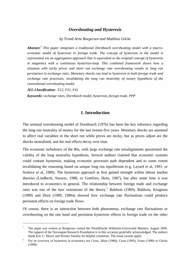
Fig. 2: Discontinuous microeconomic hysteresis loop for a single firm j
exporting
qtinactive
jαjβ
band of inaction
(exittrigger)
variableunitcosts
of firm j
(entrytrigger)
state of activity of an exporting firm j
costs costsexit entry
βExit for <tq j
αEntry for >tq j
exchange rate(price of FX)
jε
Since hysteresis effects are based on the decisions of single firms, foreign trade hysteresis is
mainly examined in a microeconomic framework. In a micro view, hysteresis implies a
difference between the exchange rates, which trigger the market entry and the exit of
potentially exporting firms. The path-dependence occurs discontinuously when "passing" the
respective rates. This pattern is illustrated in Fig. 2. Consider an exporting firm j. Let the
exchange rate q denote the home currency price of foreign exchange. Without any market
entry or exit costs a definite exchange rate εj exists where the variable unit costs are exactly
covered. Without any sunk entry and exit costs a devaluation (i.e. increase of q) passing εj
will trigger a market entry, and analogously, a revaluation below εj triggers an exit. However,
if a firm has to bear sunk market entry costs it will enter the market only if these extra costs
are covered. Consequently, the entry exchange rate trigger αj exceeds the variable cost rate εj.
5 An incomplete exchange rate pass-through is presumed, i.e. the foreign prices for exported goods do not
change in proportion to the exchange rate variation. Thus, for exchange rate alterations, the exporting firmshave to bear revenue changes in their own currency. For a model explaining this pricing to market behaviourbased on a long run optimisation see Borgersen (2001).

Borgersen / Göcke: "Overshooting and Hysteresis" 5
Analogously, an active firm will exit only if losses exceed the exit costs (e.g. resulting from
firing the staff). Thus, the exchange rate βj that triggers an exit is below εj. Summarising, the
consideration of sunk entry/exit costs produces a difference between the entry and the exit
triggers: a ’band of inaction’ with the extent (βj – αj) results.6 Inside this interval the current
exchange rate is not sufficient to determine the current state of the firm's activity. Dependent
on the past exchange rate path, two different equilibria are possible in the band between αj
and βj. A discontinuous switch between the two equilibria only occurs when the triggers are
passed. If a temporary exchange rate alteration leads to a switch, a permanent effect on
foreign trade activity remains: this after effect is technically called ’remanence’; it is the
constituting feature of hysteresis. However, the remanence effect is not irreversible (opposed
to a "ratchet effect"), since a second temporary change into the opposite direction can induce
a reversal switch leading to the initial situation.7
The microeconomic exporting behaviour of a single firm (as illustrated in Fig. 2) is
determined by a non-continuous hysteresis loop (characterised as a ’non-ideal relay’). The
qualitative characteristics of this stylised pattern remain the same if the optimisation problem
of the firm is extended to a multi-period optimisation, including a consideration of the
advantages of current activity for future costs. Even a situation with uncertainty – introducing
an option value of a 'wait-and-see strategy' – will result in the same shape of the supply
pattern. However, the option value effects will amplify the core sunk costs of entry or exit and
lead to a widening of the band-of-inaction, thus reinforcing the hysteresis property (Dixit,
1989, 1989a, and Belke, Göcke, 1999).
2.2 Aggregation and hysteresis on the macroeconomic level
In this section we apply a Mayergoyz (1986) aggregation procedure which allows an
aggregation of heterogeneous single firms, each characterised by a micro hysteresis loop,
resulting in a continuous macro loop of overall exports.8 The path dependence of the
aggregate system can be illuminated using a graphical representation of the heterogeneous
firms by their entry and exit triggers. Each potentially exporting firm is characterised by their
αj/βj-set of entry and exit trigger exchange rates. In an α/β-diagram [see Fig. 3 (a)] all α/β-
points are located in a triangle area above the 45°-line, since αj ≥ βj. The aggregation
procedure is done without any serious restriction of heterogeneity in the cost structure
between the firms. Points on the 45°-line mark the firms without any sunk costs. The distance
6 This is referred to as the “hysteresis band” by Baldwin (1988).7 See Hule (2000) for a sophisticated definition of irreversibility.8 For a more detailed description of the aggregation procedure see Amable et al (1991, 1994), Cross (1994) or
Göcke (1994).

Borgersen / Göcke: "Overshooting and Hysteresis" 6
from the origin is determined by variable unit costs εj. The extent of the sunk costs establishes
the north-west-distance of the αj/βj-set to the (α = β)-45°-line.
Assume an initial situation in point A [in Fig. 3 (a)] with a preceding time path of the
exchange rate that has created an area containing all actively exporting firms S+ (and,
correspondingly, an area of inactive firms S–). The area of S+ summarises the aggregate
exports X of the economy. As a simplifying assumption, S+ has an upper borderline towards
S– with a negative slope equal to one. Moreover – for illustration purposes – in order to imply
a one-to-one correspondence between aggregate reaction and the geometrical area, the
heterogeneous firms are assumed to be continuously and equally distributed in the α ≥ β-
triangle.9
Fig. 3: Active (heterogeneous) firms dependent on the exchange rate
(a) initial situation (b) after a 'loading-unloading cycle'
α α = β
βq0
α α = β
β
q0
S+
1
2
q0
entry trigger
exchange rateexit trigger
area ofactive firms
area ofinactive firms
S_
A
q
q q0 1q
A
C BD
F
E
G2q
S+
For an increase of the exchange rate from q0 → q1 (i.e. for a depreciation of the domestic
currency), some previously inactive firms enter the foreign market. This reaction is
represented in Fig. 3 (b) by an expansion of S+ by the triangle ABC (i.e. by an upward shift of
the horizontal S+-S–-borderline CB). A subsequent reversal of the exchange rate back to the
initial level q1 → q0 results in an exit of the firms represented by the triangle ABE (along the
vertical line AE). Although the exchange rate has regained its initial level, some firms that
have entered the foreign market during the period of depreciation, will stay: the triangle AEC
represents this persistent macroeconomic remanence effect. In order to obtain the initial level
of aggregate exports X0, a further decrease beyond the initial exchange rate is necessary. For
9 This assumption does not change the essential qualitative features of the aggregate macro-hysteresis loop.
However, the curvature of the macro loop depends upon the distribution of the firms. Under the assumptionof continuously distributed firms, a continuous macro loop can be derived.
Borgersen / Göcke: "Overshooting and Hysteresis" 7
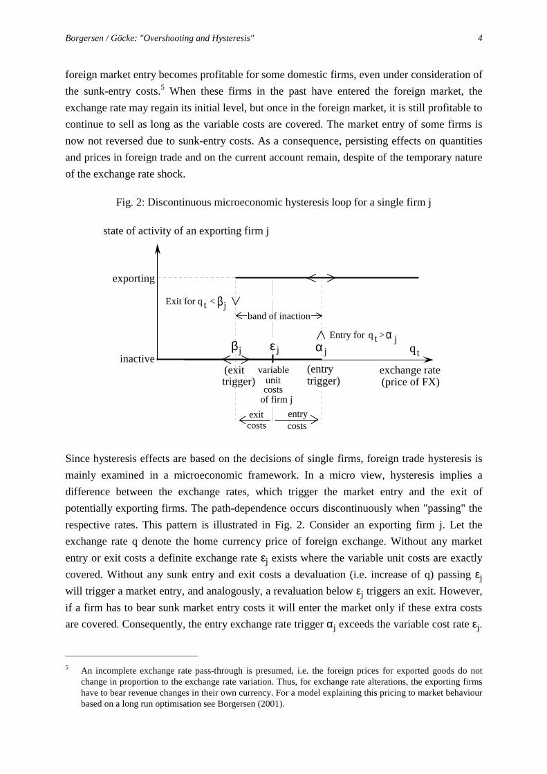
q2 the triangle AFG of initially active firms which subsequently have left the market equals
the area FDC of remanent firms that have entered during the depreciation but which have not
yet re-exited. Analogously to magnetics, we call this extra change (q2 – q0) of the forcing
variable which exceeds the reversal of the impulse the ’coercitive (force)’.
Fig. 4: Continuous macroeconomic hysteresis loop
q0 q1
X
q2 q
aggregate
exchangerate
exports
X 0
X1
X2
A’
B’
E’
H’
G’
coercitive
remanence
The effects of the exchange rate sequence q0 → q1 → q0 → q2 on aggregate exports are
depicted in Fig. 4. The initial impulse q0 → q1 leads to an increase of exports of X0 → X1. The
exchange rate reversal q1 → q0 results in a level of export of X2 > X0. I.e. a hysteretic
remanence effect (X2 – X0) occurs. In order to reach the initial export level X0 the exchange
rate has to attain q2 < q0, with the difference (q2 – q0) being the coercitive force.10 The
coercitive shows the opposite sign compared to the initial exchange rate impulse. An initial
overshooting depreciation (appreciation) is thus followed by a long run equilibrium
appreciation (depreciation).
The differences between the micro loop in Fig. 2 and the aggregate macro loop in Fig. 4 are
obvious. In the case of micro hysteresis only two states are possible. A jump between these
two non-continuously linked equilibria only occurs with the passing of certain thresholds. The
continuous macro loop results from aggregation over a high number of heterogeneous micro
elements. Due to the lack of thresholds and discontinuities, even small changes in the
exchange rate can have durable effects on the aggregate level.
Under the simplifying assumption of equally distributed firms, a geometrical interpretation of
the rectangular triangles ABC, ABE, AFG, and FDC is possible. In this case, an application of
10 A reversal of the effects of the temporary exchange rate alteration requires an even further decrease of the
exchange rate, as depicted with the path G’A’H’ in Fig. 4.

Borgersen / Göcke: "Overshooting and Hysteresis" 8
the theorem of Pythagoras results in the following relation between the initial impact (q1 – q0)
and the coercitive force c1 = (q2 – q0):11
(1) c1 = – ( 2 – 1) · (q1 – q0) = – 0.4142 · (q1 – q0)
However, under more general distribution assumptions, the factor between c1 and (q1 – q0)
would be different and generally not constant with respect to the size of (q1 – q0). In the
following we will apply a more general formulation of the coercitive effect, but remain the
linearity assumption, through a constant factor χ relating the coercitive to the initial impact:
(2) c1 = – χ · (q1 – q0) with: χ ≥ 0
So far, the logic of micro- and macro-hysteresis is explicitly outlined only for the domestic
exporters. Of course, an identical logic applies for the domestic imports, i.e. for foreign firms
considering to enter or to leave the domestic market in the presence of sunk costs. Hence, the
statements concerning the qualitative features of the macro loop apply for the aggregate
imports of a country and for the entire current account as well. Thus, of course, the impulse
and coercitive force relation in (2) can be applied to the current account as well.
By including the macro-hysteretic relationship into a macroeconomic overshooting model, the
effect of temporary fluctuations on the long run equilibrium exchange rate can be derived.
The model allows for a path dependent current account impact on demand, prices and
exchange rates, invalidating the hypothesis regarding the long run neutrality of money.
3. The overshooting model containing hysteresis in foreign trade
3.1 The money and the international capital market
Our starting point is a conventional sticky price model, along the lines of Dornbusch (1976).
We assume a small open economy, facing a given world market interest rate and perfect
capital mobility. The interest parity condition is assumed to hold. The hysteresis model
explains the foreign trade structure of the economy, i.e. the dynamic relation between real
exchange rates and the current account is characterised by a macro-hysteresis loop as
illustrated in Fig. 4. Since hysteresis is at first a goods market phenomenon, the description of
the money and capital market remains the same as in Dornbusch (1976). Hysteresis is
introduced to the model via the goods market, but shows repercussion effects on the
equilibrium of the other markets.
The money market determines the domestic interest rate and is described by a conventional
equilibrium condition, where the real money supply (M/P) equals the real money demand.
11 See the appendix for the derivation.

Borgersen / Göcke: "Overshooting and Hysteresis" 9
Demand is increasing in real income (Y) and decreasing in the interest rate (r). Small letters
represent natural logs. To keep the notification simple, an explicit time index ’t’ is suppressed.
The equilibrium condition equals:
(3) m – p = – λr + φy
In order to capture domestic price effects, the nominal spot exchange rate e (as log of the
nominal price of foreign exchange), and the log of the real exchange rate q is explicitly
distinguished. The world market price is assumed fixed (and normalised: ln(P*) = 0), so that
the real exchange rate is equal to:
(4) q = e – p
The expected rate of nominal depreciation is adaptively adjusted with reference to the steady
state equilibrium e–. Note that in the case of hysteresis, the equilibrium is not unique but path-
dependent. This is the essential difference to the original Dornbusch (1976) overshooting
model. The expected rate of exchange rate depreciation e°e is assumed proportional to the
discrepancy between the actual rate and the long run equilibrium exchange rate. The speed of
adjustment coefficient θ is (for the moment) exogenously given:
(5) e°e ≡
de
dt
e = θ · (e– – e) with: θ ∈ [0,1]
Capital mobility is characterised by an interest parity condition that implies perfect
substitutability between assets denominated in domestic and foreign currency. The interest
rate is approximated by r ≈ ln(1 + i) . The world market interest rate is given by r*, and is fixed
due to the small country assumption.
(6) r = r* + e°e = r* + θ · (e– – e)
Combining eqs. (3), (5) and (6) leads to a relationship between the nominal spot rate, the price
level and the long run equilibrium exchange rate, given the money market clearance and the
asset market equilibrium condition:
(7) m – p = φy – λ · [r* + θ · (e– – e)]
In the long run equilibrium, the expectations are correct (e = e–) and the expected rate of
depreciation is zero (r = r*). Thus, the steady state price level is:
(8) p– = m – φy – λr*
The combination of eqs. (7) and (8) results in:
(9) e = e– – 1
λθ · (p – p–)

Borgersen / Göcke: "Overshooting and Hysteresis" 10
Thus, the nominal exchange rate is determined by the price level. The price determines the
interest rate via the real money supply; and via interest parity the nominal exchange rate is
set.
3.2 The goods market containing hysteresis in foreign trade
Now we have to implement hysteresis effects into the goods market. The goods market is
characterised by a real income which is fixed by the supply side (y = const.).12 The price
pressure in the model depends upon real demand. The log demand function d = ln(D) contains
normal income and substitution effects:
(10) d = µ + δ · (q – q–) + γ · y – σ · r
The inflation rate p° is assumed to be proportional to an excessive demand factor:
(11) p° ≡ dpdt = π · ln(D/Y) = π · (d – y)
An exogenous shock which leads to a temporary deviation from an initial equilibrium level of
the real exchange rate q–0 will result in a different new equilibrium level q–1 as far as hysteretic
remanence effects on the current account occur. The difference between the old and the new
equilibrium of the real exchange rate is given with the coercitive force c1. It guarantees that
the initial (equilibrium) level of the current account will be regained in the new steady state.
The real exchange rate in the first moment after the shock (t = +0) – i.e. the overshooting
exchange rate after the impact effect – is stated as q1. Hence, the initial impulse is (q1 – q–0)
and the new equilibrium level of the real exchange rate is:
(12) q–1 = q–0 + c1 = q–0 – χ · (q1 – q–0) with the coercitive force: c1 = χ · (q1 – q–0)
The real demand after a shock is d = µ + δ · (q – q–1) + γ · y – σ · r . Thus, the change of the
price level is now given as:
(13) p° = π · {µ + δ · [e – p – q–0 + χ · (q1 – q–0)] + (γ – 1) · y – σ · r}
An actual remanence and coercitive effect as stated in eq. (12) requires a real entry and/or exit
of exporting firms into the foreign market. Thus, although the supply is assumed to be fixed,
the current account is not fixed. When q rises in the course of a real depreciation, firms will
enter the foreign market, as the real exchange rate change brings about a rise in unit revenues
converted into the home currency. At the same time, the unit revenue on the domestic market,
i.e. the price, is sticky and lags behind. Thus, the firms will first serve the international market
12 Later in the paper we will show that the equilibrium real exchange will show hysteresis effects. Of course a
shift in the terms of trade has an effect on the value added by the economy (i.e. on output y). As asimplification, these effects are neglected and the output is assumed to be constant.

Borgersen / Göcke: "Overshooting and Hysteresis" 11
and then the domestic market in a situation with excessive demand. Consequently, excessive
demand is a phenomenon on the domestic goods market, driving the sticky domestic price
level p.
In the long run, a goods market equilibrium implies p° = 0 . With r = r* the new long run
equilibrium of the nominal exchange rate after a shock ( e–1 = q–1 + p–1 ) is under consideration of
the coercitive characterised by:
(14) e–1 = p–1 + q–0 – χ · (q1 – q–0) – 1δ · [µ + (γ – 1) · y – σ · r*]
Using eq. (12), the definition of the new equilibrium of the nominal exchange rate e–1 = q–1 + p–1
can be reformulated with explicit consideration of the coercitive. In the first moment after the
shock the nominal exchange rate "jumps" to e1 while the price level is sticky and, for the
present, remains on its initial level p1 = p–0 .
(15) e–1 = e–0 – p–0 – χ · (q1 – q–0) + p–1 = e–0 – p–0 – χ · (e1 – p–0 – e–0 + p–0) + p–1
e–1 = e–0 – χ · (e1 – e–0) + p–1 – p–0
Reformulating eq. (9) yields:
(16) e1 = e–1 – 1
λθ · (p–0 – p–1) ⇒ e–1 = e1 + 1
λθ · (p–0 – p–1)
Equating eq. (15) and (16) gives the instantaneous jump of the nominal exchange rate directly
after the shock:
(17) (e1 – e–0) = 1 + 1/(λθ)
1 + χ · (p–1 – p–0)
The price dynamics can be derived based on eq. (13), by inserting e1 as implicitly given in eq.
(17), via using e–1 corresponding to eq. (14), by substituting e as stated in eq. (9), and under
application of the definition equations q1 = e1 – p1 and q–0 = e–0 – p–0 as well the sticky price
condition p1 = p–0 . The result shows that the price dynamics are described as an autonomous
first order differential equation of the form p°(p); i.e. the only endogenous variable that
determines the change of the price is the price level itself.
(18) p° = – υ · (p – p–1) where: υ ≡ π ·
δ + σθ
λθ + δ
Eq. (18) is equivalent to Dornbusch's (1976, p. 1165) eq. (10). However, the interpretation is
novel. Due to hysteresis effects, the new equilibrium level p–1 is different compared to a
situation without hysteretic coercitive effects (i.e. when χ = 0). In a situation without
hysteresis, the equilibrium level of the real exchange rate (which determines the long run

Borgersen / Göcke: "Overshooting and Hysteresis" 12
level of p and e) is unique; i.e. long run changes of the nominal variables e and p must be
proportional and no real effect will occur in the long run. Thus, monetary shocks are neutral
in the long run. However, in a situation with hysteresis in foreign trade (χ > 0), the long run
effects on p and e are not proportional, since the real exchange rate q changes. Hystereses
implies long-run non-neutrality of monetary disturbances, and – even in the long run – a
violation of Purchasing Power Parity.
The solution of eq. (18) is straightforward (under consideration of the initial condition
p(t = 0) = p–0 ):
(19) p(t) = p–1 + (p–0 – p–1) · exp(– υ · t)
Substitution of p(t) in eq. (9) e(t) = e–1 – (1/λθ) · (p(t) – p–1) (with: e1 = e–1 – (1/λθ) · (p–0 – p–1))
gives the time path of the nominal exchange rate:
(20) e(t) = e–1 – 1
λθ · (p–0 – p–1) · exp(– υ · t) = e–1 + (e1 – e–1) · exp(– υ · t) ⇒
dedt ≡ e° = – υ · (e1 – e–1) · exp(– υ · t) = υ · (e–1 – e(t))
3.3 Rational expectations
A perfect foresight path requires the actual exchange rate dynamics e° to equal the expected
rate of nominal depreciation as stated in eq. (5). Thus, the adaptive model shows rational
expectations if the following constraint applies to the adaptive expectations coefficient θ(Dornbusch (1976, p. 1167)):
(21) e°e =! dedt ⇒ θ =
! υ ≡ π ·
δ + σθ
λθ + δ ⇒
= 2
+ +π σ π δ λ + + +π2 σ2 2 π2 σ δ λ π2 δ2 λ2 4 π δ λλθ(rat.)
3.4 A monetary shock
As an example, we now discuss the effects of a monetary shock. The money supply is once
for forever increased from an initial level m0 to m1 by the increment dm ≡ m1 – m0. According
to eq. (8) the long run equilibrium price level after the monetary shock is:
(22) p–1 = m1 – φy – λr* (and: p–0 = m0 – φy – λr* )
⇒ dp–m ≡ p–1 – p–0 = dm

Borgersen / Göcke: "Overshooting and Hysteresis" 13
Inserting this long run price effect into eq. (17) gives the impact effect on the exchange rate,
i.e. the jump in the first moment after the monetary shock:13
(23) de1 = e1 – e–0 = 1 + 1/(λθ)
1 + χ · dm
Since the prices are sticky, the real exchange rate jump equals the nominal impact effect in the
first moment after the shock (dq1 = q1 – q–0 = de1). As can be seen from eq. (23), an interaction
between hysteresis effects and exchange rate overshooting exists. The higher the persistence
effects (the higher χ), the lower is the new long run equilibrium rate of the real exchange rate
q–1 and, thus, the lower is the first period jump of the exchange rate (dq1 = de1) immediately
after the shock. Hence, the overshooting of the exchange rate is reduced via long run
coercitive force effects introduced by hystereis in foreign trade.
With eqs. (15), (22) and (23) the hysteretic long run equilibrium effect on the nominal
exchange rate can be calculated:
(24) e–1 = e–0 – χ · (e1 – e–0) + p–1 – p–0 = e–0 – χ · de1 + dp–m
⇒ de–m ≡ e–1 – e–0 = λθ – χ
λθ · (1 + χ) · dm
In a situation without hysteresis (χ = 0) the long run effect on the nominal exchange rate is
de–m;χ=0 = dm = dp , thus, for χ = 0 there is no long run effect on the real exchange rate q, i.e.
due to long-term monetary neutrality the PPP holds. However, in a situation with hysteresis
effects in foreign trade (χ > 0), the monetary expansion has a long run effect on the real
exchange rate. The real depreciation in the short run ultimately results in a real appreciation in
the long run (for dm > 0 ⇒ dq1 > 0 and dq–m < 0):
(25) dq–m ≡ q–1 – q–0 = de–m – dp–m = – χ · (1 + λθ)λθ · (1 + χ)
· dm
3.5 A graphical illustration of the dynamics
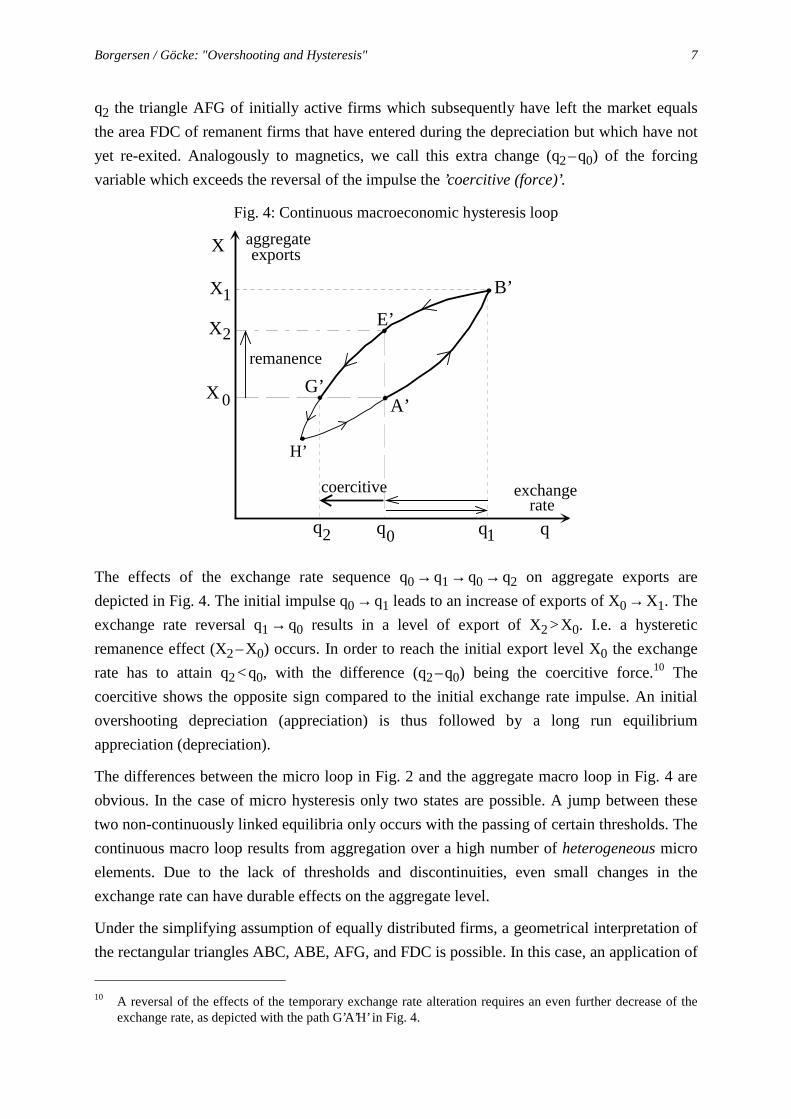
The dynamics of the hysteretic system can be illustrated by a two-dimensional (e,p)-plane
using the phase diagram technique (see Fig. 5).14 The line QQ delineates eq. (9). In the case of
rational expectations (i.e. for θ = θrat) the line QQ represents the stable saddle-ath of the
system. As an extra information the (e° = 0)-isokine as implicitly given in eq. (9) and the
(p° = 0)-isokine as derived from eq. (13) are depicted. The initial equilibrium situation is
represented by point A. As the monetary expansion has a positive long run effect on the price
13 For χ = 0, our eq. (23) reduces to Dornbusch's (1976, p. 1169) eq. (16).14 For the corresponding graph in a situation without hysteresis effects see Dornbusch (1976), p. 1169.
Borgersen / Göcke: "Overshooting and Hysteresis" 14
level and as the real exchange rate is reduced in the long run by the temporary devaluation,
the 45°-line characterising a constant real exchange rate based on its definition (q–0;1 = e – p) is
shifted to the left, due to the hysteretic coercitive force. This dampens the impact effect on the
exchange rate. The short run impact effect is depicted via the jump from A to point B in Fig.
5. The adjustment to the new long run equlibrium (from B to point C) takes place along the
new saddle-path Q1Q1.15
Fig. 5: Effects of a monetary expansion in a phase diagram
p
45°
e
p0
–
p1
–
A
C
Q
Q
0
0Q1
Q1
B
q1
– q0
–
q1
– q0
– e0– e1e1
–
coercitive
dm
(e = 0)°1
(e = 0)°0
(p = 0)°0
(p = 0)°1
D
E
4. A numerical example
A simulation of the model can illustrate the process of hysteresis, and the persistent real
exchange rates. The parameters of the model are set to: χ = 0.4, π = 0.5, δ = 3, σ = 4, µ = 1, λ = 4,
φ = 0.25, γ = 0.8. The initial situation in the economy is given as: m0 = 1, y0 = 1, r* = 0.1, e0 = 1.
The economy is assumed to be in equilibrium initially, where the money market is given as
p0 = p–0 = m0 – φy0 + λr* = 1.15 and q0 = q–0 = e0 – p0 = – 0.15. The rational expectation coefficient
θ(rat.) equals the price adjustment coefficient υ: θ(rat.) = υ = 2.17260349. Both, the level of
production and the foreign interest rate are assumed fixed – that is dy = dr* = 0.
Consider a monetary expansion equal to dm = m1 – m0 = 0.5. The new equilibrium price level
is p–1 = p(t = ∞) = 1.65. The nominal exchange rate immediately before the monetary shock (in
15 If q–0 were the unique equilibrium PPP level of the real excahnge rate in the standard case without hysteresis,
the monetary shock would result in a jump to point D in Fig. 5. Subsequently, the transitional dynamicstowards the unique q–0-equilibrium line in point E would take place on the saddle-path DE.

Borgersen / Göcke: "Overshooting and Hysteresis" 15
t = – 0) is e0 = e(t = – 0) = 1. In the first moment after the shock (t = + 0) it equals
e1 = e(t = + 0) = 1.398239034. The new long run equilibrium exchange rate is e–1 = e(t = ∞) =
1.340704387, making the first moment overshooting over its long run equilibrium level equal
to e1 – e–1 = 0.3982390337. The differential equations reflecting the speed of adjustment of the
price level and its solution can be calculated as:
(26) p° = dpdt = –2.172603940 p(t) + 3.584796501
p(t) = 1.65 – 0.5 · exp(–2.17260394 · t)
e(t) = 1.340704387 + 0.05753464665 · exp(–2.17260394 · t)
Fig. 6: Reaction of the sticky price level p and of the
overshooting nominal exchange rate e on a monetary expansion
t
21.510.50
1.6
1.5
1.4
1.3
1.2
p(t)
new steady state
p–0
p–1
t
21.510.50
1.3
1.2
1.1
e(t)
t = –0 (initial situation)
new steady state
e0–
e1–
e1
impact effect
The slow price adjustment and the excessive overshooting of the nominal exchange rate
initiated by the monetary expansion are illustrated in Fig. 6. corresponding to the stylised
representation in Fig. 5, the simulated saddle-path dynamics are depicted in a standard (e,p)-
diagram in In the new long run equilibrium p(t = ∞) = 1.65 and e(t = ∞) = 1.340704387, the total
equilibrium effect on domestic prices, the nominal exchange rate and the resulting negative
long run effect on the real exchange rate are:
(27) ≡ – = p(t = ∞) – p(t = 0) = dm = 0.5 > 0
≡ – = e(t = ∞) – e(t = – 0) = 0.340704387 > 0
= – = – 0.159295613 < 0
These results imply that with a monetary expansion the price effects are neutral in a
conventional sense. However – since there is a under-proportional nominal exchange rate
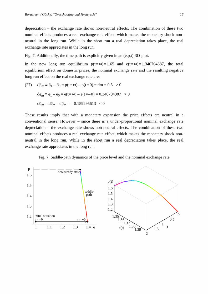
Borgersen / Göcke: "Overshooting and Hysteresis" 16
depreciation – the exchange rate shows non-neutral effects. The combination of these two
nominal effects produces a real exchange rate effect, which makes the monetary shock non-
neutral in the long run. While in the short run a real depreciation takes place, the real
exchange rate appreciates in the long run.
Fig. 7. Additionally, the time path is explicitly given in an (e,p,t)-3D-plot.
In the new long run equilibrium p(t = ∞) = 1.65 and e(t = ∞) = 1.340704387, the total
equilibrium effect on domestic prices, the nominal exchange rate and the resulting negative
long run effect on the real exchange rate are:
(27) dp–m ≡ p–1 – p–0 = p(t = ∞) – p(t = 0) = dm = 0.5 > 0
de–m ≡ e–1 – e–0 = e(t = ∞) – e(t = – 0) = 0.340704387 > 0
dq–m = de–m – dp–m = – 0.159295613 < 0
These results imply that with a monetary expansion the price effects are neutral in a
conventional sense. However – since there is a under-proportional nominal exchange rate
depreciation – the exchange rate shows non-neutral effects. The combination of these two
nominal effects produces a real exchange rate effect, which makes the monetary shock non-
neutral in the long run. While in the short run a real depreciation takes place, the real
exchange rate appreciates in the long run.
Fig. 7: Saddle-path dynamics of the price level and the nominal exchange rate
e1.41.31.21.11
p
1.6
1.5
1.4
1.3
1.2
saddle-
t = –0 t = +0initial situation
new steady state
path
1.381.39
1.371.36
1.35
21.5
10.5
0
1.6
1.5
1.4
1.3
1.2
p(t)
e(t) t
Borgersen / Göcke: "Overshooting and Hysteresis" 17
5. Conclusion
The overshooting model of Dornbusch (1976) is often used to show the consequences of short
run exchange rate fluctuations in a situation when the long run neutrality of money hypothesis
holds. The combination of sticky prices and flexible asset markets produces real effects in the
short run, but as prices adjust the effects decay over time. Here however, the situation with
sticky prices and overshooting exchange rate effects is shown to provide a framework where
long run persistent effects in exchange rates and foreign trade flows can come about. The long
run neutrality of money is invalidated, as short run fluctuations can cause long run persistence
and variability. The hysteresis approach provides a fundamental attack on the long run
neutrality hypothesis, as it describes the economic system as one where no unique long run
equilibrium exists. Via merely introducing one extra parameter χ for the hysteretic coercitive
effect on the long run equilibrium level of the real exchange rate, the model also shows in a
very simple way how – in contradiction to Baldwin and Lyon (1994) – passing of extreme
values is not necessary to produce hysteresis in a sticky price framework. But again, a
positive demand shock which leads to a temporary exchange rate depreciation is followed by
a persistent appreciation. The initial overshooting effect and the long run coercitive effect are
related. The more severe the overshooting, the more severe is the persistence on the long run
equilibrium. And, at the same time, the stronger the long run persistence effect, the weaker is
the initial exchange rate "jump". Thus, the more variable the long run solution, the less
fluctuation comes about in the short run. The degree of overshooting depends upon the size of
the initial shock, the degree of nominal price stickiness and the distribution of firms with
respect to levels of the exchange rate that triggers entry and exit. The long run persistence
depends upon the initial situation, and again the distribution of firms with respect to the entry
and exit triggers. The model also attacks the PPP hypothesis, since monetary shocks have real
effects in the long run. In our hysteresis approach the invalidity of the PPP hypothesis comes
from the functioning of the economic system itself rather than an imperfection in the system.
The continuos regime switches produce welfare costs both with respect to scrapping of sunk
costs, and to the ability to perform macroeconomic planning and stabilisation policies. With
long run variability the degree and even direction of policies might be uncertain.16
16 See Roberts, Tybout (1997) for a thorough policy discussion.

Borgersen / Göcke: "Overshooting and Hysteresis" 18
References:
Amable, B., Henry, J., Lordon, F., Topol, R. (1991): "Strong Hysteresis: An Application to ForeignTrade". OFCE Working Paper No. 9103, Observatoire Francais des ConjoncturesEconomiques, Paris.
Amable, B., Henry, J., Lordon, F., Topol, R. (1993): "Unit-Root-Hysteresis in the Wage-priceSpiral Is Not Hysteresis in Unemployment". Journal of Economic Studies 20, 123-135.
Amable, B., Henry, J., Lordon, F., Topol, R. (1994): "Strong Hysteresis versus Zero-RootDynamics". Economic Letters 44, 43-47.
Amable, B., Henry, J., Lordon, F., Topol, R. (1995): "Hysteresis revisited: A methodologicalapproach". In: Cross, R. (ed.) Unemployment, Hysteresis and The Natural Rate Hypothesis.Oxford/NewYork, 26-38.
Baldwin, R. (1988): "Hysteresis in Import Prices: The Beachhead Effect". American EconomicReview 78, 773-785
Baldwin, R. (1989): "Sunk-Cost Hysteresis". NBER Working Paper No. 2911.
Baldwin, R. (1990): "Hysteresis in Trade". In: Franz, W. (ed.), Hysteresis Effects in EconomicModels, Heidelberg, 19-34 (also published in: Empirical Economics 15 (1990), 127-142).
Baldwin, R., Krugman, P. (1989): "Persistent Trade Effects of Large Exchange Rate Shocks".Quarterly Journal of Economics 104, 635-654.
Baldwin, R., Lyons, R. (1994): "Exchange Rate Hysteresis? Large versus Small PolicyMisalignments". European Economic Review 38, 1-22.
Belke, A., Göcke, M. (1999): "A Simple Model of Hysteresis in Employment Under Exchange RateUncertainty". Scottish Journal of Political Economy 46, 260-286.
Borgersen, T. (2001): "Exchange Rate Pass Through and the Planning Horizon of Firms". AgderUniversity College, Working paper, forthcoming.
Branson, W.H. (1977): "Asset Markets and Relative Prices in Exchange Rate Determination".Sozialwissenschaftliche Annalen des Instituts für Höhere Studien 1, 69-89.
Brokate, M., Sprekels, J. (1996): "Hysteresis and Phase Transitions". In: Marsden, J.E, Sirovich, L.,John, F (eds.) Applied Mathematical Sciences 121, Springer, New York.
Cross, R. (1993): "On the Foundations of Hysteresis in Economic Systems". Economics andPhilosophy 9, 53-74.
Cross, R. (1994): "The Macroeconomic Consequences of Discontinous Adjustment: SelectiveMemory of Non-Dominated Extrema". Scottish Journal of Political Economy 41, 212-221.
Cross, R., Allan, A. (1988): "On the History of Hysteresis". In: Cross, R. (ed.), Unemployment,Hysteresis and the Natural Rate Hypothesis, Oxford/New York, 26-38.
Dixit, A. (1989): "Hysteresis, Import Penetration, and Exchange Rate Pass-Through", QuarterlyJournal of Economics 104, 205-228.
Dixit, A. (1989a): "Entry and Exit Decisions under Uncertainty". Journal of Political Economy 97,620-638.
Dornbusch, R. (1976): "Expectations and Exchange Rate Dynamics". Journal of Political Economy84, 1161-1176.
Franz, W. (1990): "Hysteresis in Economic Relationships: An Overview". In: Franz, W. (ed.),Hysteresis Effects in Economic Models, Heidelberg, 1-17 (also published in: EmpiricalEconomics 15 (1990), 109-125).

Borgersen / Göcke: "Overshooting and Hysteresis" 19
Froot, K.A., Klemperer, P.D. (1989): "Exchange Rate Pass-Through When Market Share Matters".American Economic Review 79, 637-654.
Giovannetti, G., Samiei, H. (1996): "Hysteresis in Exports". CEPR Discussion Paper No. 1352,London.
Goldberg, P.K., Knetterer, M.M. (1997): "Goods Prices and Exchange Rates: What Have WeLearned?" Journal of Economic Literature 35, 1243 -1272.
Göcke, M. (1994): "Micro- and Macro Hysteresis in Foreign Trade". Aussenwirtschaft -Schweizerische Zeitschrift für internationale Wirtschaftsbeziehungen 49, 555-578.
Göcke, M. (1999): "Types of Hysteresis applied in Economics". Universtity of Münster, DiscussionPapers in Economics No. 292.
Gottfries, N., Horn, H. (1987): "Wage Formation and the Persistence of Unemployment". EconomicJournal 97, 877-884.
Han, H-Y. (1991): "The Sunk Cost Hysteresis in International Trade". Kyongje-yon'gu – TheHanyang Journal of Economic Studies 12, 241-263.
Harris, R.G. (1993): "Exchange Rates and Hysteresis in Trade", in: The Exchange Rate and theEconomy, proceedings of a conference held at the Bank of Canada, 22-23 June 1992,Ottawa, 361-396.
Hule, R. (2000): Irreversibilität in der Ökonomik. Ph.D. Diss. (University of Innsbruck, 1996),Frankfurt.
Krasnosel’skii, M.A., Pokrovskii, A.V. (1989): Systems with Hysteresis, Springer/Berlin.
Layard, R., Nickell, S., Jackman, R. (1991): Unemployment, Macroeconomic Performance and theLabour Market. Oxford University Press.
Lindbeck, A., Snower, D. (1988): The Insider Outsider Theory of Employment and Unemployment.Cambridge Mass., MIT Press.
Ljungqvist, L. (1994): "Hysteresis in International Trade: a General Equilibrium Analysis". Journalof International Money and Finance 13, 387-399.
McClausland, W.D. (2000): "Exchange Rate Hysteresis from Trade Account Interaction". TheManchester School 68, 113-131.
Mayergoyz, I.D. (1986): "Mathematical Models of Hysteresis". IEEE Transactions on Magnetics 22,603-608.
O’Shaughnessy, T. (2000): "Hysteresis in an Open Economy Model". Scottish Journal of PoliticalEconomy 47, 156 -182.
Roberts, M., Tybout, R. ( 1997): "The Decision to Export in Colombia: An Empirical Model of Entrywith Sunk Costs". American Economic Review, Vol.87, No 4 .
Soskice, D., Carlin, W. (1989): "Medium-run Keynesianism: Hysteresis and Capital Scrapping". In:Davidson, P., Kregel, J. (ed.): Macroeconomic Problems and Policies of IncomeDistribution, Edward Elgar Press.
Sullivan, T. (1996): "Hysteresis in Trade and Export Supply: An Econometric Investigation UsingFirm-level Panel Data". Ph.D. Diss., Georgetown University.
van Garderen, Kes J., Lee, K., Pesaran, M. Hashem (1997): "Cross-Sectional Aggregation of Non-Linear Models". DAE Working Paper No. 9803, University of Cambridge – Department ofApplied Economics.

Borgersen / Göcke: "Overshooting and Hysteresis" 20
Appendix:
The relation between the first impact (q1 – q0) and the adjustment (q2 – q1) is aquivalent to the
relation between the distance AB [between the points A and B in Fig. 3 (b)] and the distance
GB on the 45°-line:
(28) GB / AB = (GA + AB) / AB = (q1 – q2) / (q1 – q0)
⇒ GA / AB = (q0 – q2) / (q1 – q0)
The space of the rectangular triangle AFG equals the space of the triangle FDC of remanent
firms, if the triangle GBD and the triangle ABC have the same space. Thus, both hypotenuses
GB and CB show equal length as well as all catheds do (AB and AC of ABC, and DG and DB
of GBD). Based on the theorem of Pythagoras, the following holds:
(29) GB2 = 2 AB2 ⇒ (GA + AB)2 = 2 AB2 ⇒ GA = ( 2 – 1) · AB
A combination of eqs. (28) and (29) yields:
(30) ( 2 – 1) = (q0 – q2) / (q1 – q0) ⇒ c1 = (q2 – q0) = – ( 2 – 1) · (q1 – q0)