well test interpretation using ... - stanford … understanding well test results. it has b een...
TRANSCRIPT

WELL TEST INTERPRETATION
USING
LAPLACE SPACE TYPE CURVES
By
Marcel Bourgeois
Elf Aquitaine
April 1992
Contents
1 Introduction 1
2 Mathematical Background 3
2.1 Considerations of Dimension : : : : : : : : : : : : : : : : : : : 3
2.2 Flowrate Deconvolution : : : : : : : : : : : : : : : : : : : : : 5
2.3 Initial And Final Value Theorem : : : : : : : : : : : : : : : : 7
2.4 Semilog Behavior : : : : : : : : : : : : : : : : : : : : : : : : : 8
3 Applications 11
3.1 Forward Laplace Transform : : : : : : : : : : : : : : : : : : : 11
3.2 Type Curves : : : : : : : : : : : : : : : : : : : : : : : : : : : : 17
3.3 Treatment Of Wellhead Flowrate Variation : : : : : : : : : : : 26
3.4 Buildup With No Measurement Prior To Shut-In : : : : : : : 30
3.5 Numerically Stable Wellbore Storage Removal : : : : : : : : : 34
3.6 Pressure Dependant Wellbore Storage : : : : : : : : : : : : : : 39
3.7 Nonlinear Regression in Laplace Space : : : : : : : : : : : : : 42
4 Conclusion 45
4.1 Nomenclature : : : : : : : : : : : : : : : : : : : : : : : : : : : 47
4.2 Subscripts and Superscripts : : : : : : : : : : : : : : : : : : : 47
5 Appendix 51
5.1 Fortran Program : : : : : : : : : : : : : : : : : : : : : : : : : 51
5.2 Field Example : : : : : : : : : : : : : : : : : : : : : : : : : : : 52
i
Acknowledgements
This work, which summarizes 18 months of research at Stanford University, is
part of the Stanford Well Testing Industrial A�liates Program (SUPRI-D).
It was conducted under the direction of Professor Roland N. Horne, and I am
deeply appreciative of his advice, guidance and encouragement throughout
our friendly but fruitful collaboration.
I would also like to express my gratitude to ELF Aquitaine that provided
me with adequate preparation and material support for this research.
ii
Abstract
This study presents the mathematical background which justi�es the use of
Laplace space in well test analysis. It enables us to perform the whole pa-
rameter identi�cation (CD; Skin; kh; ...) in Laplace space, or at least gives
us a powerful tool to treat the pressure data in order to recognize the model
to use for the parameter identi�cation in real space. It shows a manner in
which the Laplace transform can be plotted, showing exactly the same be-
haviour as the real pressure function so the plots keep their familiar shape.
The coe�cients of the dimensionless parameters remain the same, too. This
enables us to display a new set of characteristic and easily understandable
type curves in Laplace space.
The mathematical background also sheds light on the use of the Laplace
transform to achieve owrate deconvolution, using modi�cations of earlier
techniques which had been found to be extremely sensitive to noise in the
data.
The treatments displayed are numerically stable, and it is explained why
numerical instability can occur in owrate deconvolution. The e�ectiveness
of the treatments is explained whenever possible, and the e�ect of the late-
time extrapolation is discussed as well.
The Laplace space approach provides an entirely new way of examining
and understanding well test results. It has been succesfully applied to noisy,
simulated data where a conventionnal interpretation could not illuminate
ambiguities.
iii
Chapter 1
Introduction
There are many techniques available for solving the problem of transient ow
of slightly compressible uids in porous media. One of them is the use of
the Laplace transform, which has many convenient properties (van Everdin-
gen and Hurst, Ref. [1]). Since the di�usivity equation is usually simpler in
Laplace space than in real space, solutions may be determined for most well
con�gurations, which correspond to di�erent boundary conditions. Previous
investigations, particularly Ozkan and Raghavan (Ref. [2, 3]), provide exten-
sive libraries of computable solutions to a great variety of well test problems.
The analytical solutions are therefore usually better known in Laplace space
than in real space. In addition to this, evaluating the solution in Laplace
space makes it very easy to take into account the double porosity behaviour
of a �ssured reservoir.
Despite all these advantages, the Laplace transform often remains ab-
struse and somewhat \user-unfriendly", because methods of direct interpre-
tation rely on the visualization of the solution in real space, in order to
recognize the reservoir model.
This study investigates a way of presenting the Laplace transform of the
transient wellbore pressure which makes it directly interpretable. It allows us
to create characteristic type curves, and therefore to perform model recogni-
tion in Laplace space. Eventually, the whole parameter identi�cation can be
performed in Laplace space, which reduces the need for numerical inverters.
This, as discussed in the last chapter, is interesting when the data are not
1

monotonic and the time consuming algorithm developed by Crump [4] has to
be used instead of Stehfest's algorithm [5]. Working more in Laplace space
can therefore save a lot of mathematical treatment, which is all the more
pro�table when numerous iterations are to be performed, such as in non-
linear regression, also known as automated type-curve matching (Rosa and
Horne, Ref. [6]), one of the more promising modern well test identi�cation
methods.
The new understanding of the properties of the Laplace space solutions
has enabled the development of a new method for deconvolving owrate
variations with noisy data. Basically, owrate deconvolution has a very sim-
ple expression in Laplace space for perfect data, but numerical instability,
which is inherent to the process, can cause problems. Constrained methods
(Kuchuk et al., [7]) can be used to perform deconvolution despite this insta-
bility, but this study shows a simpler and quicker treatment, even in cases
when no owrate measurements are available.
This work therefore expands our ability to solve problems of transient
ow with a simple yet powerful approach.
This work has been presented at the Society of Petroleum Engineers Fall
Meeting in Dallas (Oct.7th, 1991) as paper # 22682, and the last results
have been presented at the student paper contest during the Western Re-
gional Meeting in Bakers�eld (March 30th, 1992). It has been accepted for
publication in SPE Formation and Evaluation.
2

Chapter 2
Mathematical Background
2.1 Considerations of Dimension
With fully dimensional variables, sf is de�ned as the Laplace variable (as
opposed to the dimensionless Laplace variable traditionally noted s), after
which the de�nition of the Laplace transform is:
Lfp(t)g = p(sf ) =
Z1
t=0e�sf t p(t) dt (2:1)
The dimension of p(sf ) is therefore time � pressure, which is not very
convenient. It is much more interesting to work with the new expression,
which we will call Laplace pressure:
sf Lfp(t)g = sf p(sf ) (2:2)
This expression has the dimension of a pressure, and will therefore be
expressed in psi if oil�eld units are chosen, or in bar or Pascal . It should be
emphasized that the operator, which acting on the real pressure p(t) results
in the Laplace pressure sf � p(sf ), has a very useful linear behavior, which
will enable us to perform unit conversions or multiplications: For example,
if p0 = 1, we have sfp0(sf) = 1, and thus:
sf (a + b � p) = a + b � sfp (2:3)
3

In these equations, sf has the dimension of a reciprocal time, and the
reader should always keep in mind that large values of sf correspond to
small values of t, because the contribution of the pressure to the Laplace
integral is signi�cant only at early times if sf is large. Conversely, if the
values of sf are small, the contribution to the Laplace integral will cover the
whole time range, until late time.
It is a common approach to work with dimensionless quantities, in order
to keep familiar values even if the scale or the properties of well and reservoir
are changed, or if the unit system changes. The de�nitions are, in consistent
units:
pD =2� k h
qB ��p =
�p
�p
(2.4)
tD =k t
� � ct r2w=
t
�t
(2.5)
CD =C
2� h � ct r2w=
C
�C
(2.6)
In oil�eld units, the de�nitions are:
pD =k h
141:2 qB ��p (2.7)
tD =0:000264 k t
� � ct r2w(2.8)
CD =0:8936 C
h � ct r2w(2.9)
The relation �p = �t=�C is only true in consistent units. For the oil�eld
unit system, the equivalent relation is �p = qB=24 � �t=�c , because C is
expressed in bbl/psi and not in hr/psi.
The de�nition of the dimensionless Laplace variable is:
s = sf t=td = �t sf (2:10)
The dimensionless Laplace pressure is therefore:
4

s pD(s) = s
Z1
tD=0e�stD pD(tD) dtD =
2� k h
qB �sf �p(sf) (2:11)
The proportionality coe�cient �p between dimensionless and full dimen-
sion Laplace pressure remains the same as in real space, which is very con-
venient:
s pD(s) = sf �p(sf) =�p (2:12)
For the skin S, the dimensional pressure drop across the skin is related
to the dimensionless skin factor the following way:
�pS = �p S (2:13)
2.2 Flowrate Deconvolution
The convolution of two functions in real space is equivalent to the product of
their Laplace transforms in Laplace space. The pressure drop in the wellbore
(assuming no skin) is the convolution integral of the Kernel function K with
the derivative of the sandface owrate:
pD(tD) =
ZtD
�=0K(tD � � )
@qsfD(�)
@�d� (2:14)
Thus in Laplace space:
pD(s) = K(s) � s qsfD(s) (2:15)
Here pD is the pressure drop which actually occured due to the (vari-
able) sandface owrate qsfD (=qsf=qreference), and K is the pressure drop
which would have occured had the well been opened to ow at constant rate
(qreference) at time zero. To yield the pressure drop in the well which would
have occured if the owrate had been a Heaviside step function ( = Kernel
function), the actual Laplace pressure drop is divided by the Laplace owrate
[1, 8]:
s K(s) =s pD(s)
s qsfD(s)
(2:16)
5

To compute the pressure drop in the wellbore for a constant wellbore
storage CD and skin S, the following formula can be used, which simply
adds a skin pressure drop proportional to the actual sandface owrate:
pwD(tD) =Z
tD
�=0K(tD � � )
@qsfD(�)
@�d� + qsfD(tD) S (2:17)
In Laplace space:
s pwD(s) = s K(s) � s qD(s) + s qD(s) S (2:18)
Knowing that the sandface owrate is equal to the wellhead owrate
minus the wellbore unloading, we can say:
qsfD = qwhD � CD
@pwD
@tD(2:19)
For a unit step wellhead owrate, in Laplace space:
s qsfD = 1 � CD s2 pwD(s) (2:20)
Rearranging this, pwD can be expressed as a function of K; CD and S:
s pwD(s) =sK(s) + S
1 + CD s ( sK(s) + S )(2:21)
Conversely, to remove CD and S from a measured wellbore pressure:
s K(s) =spwD(s)
1 � CD s2 pwD(s)� S (2:22)
This relation is exact, but can be numerically unstable (due to division
by zero) for wellbore storage deconvolution, if the data are noisy or if CD
is overestimated. This important practical problem is addressed later (see
Eq. 3.58).
6

2.3 Initial And Final Value Theorem
Let us start with the initial value theorem, which is more intuitive. This
theorem is true for any function that admits a Laplace transform. It is thus
applicable to the owrate and, what is of most interest for us, to the pressure,
dimensionless or not. If the indicated limit exists, then:
limt!0
f (t) = limsf!1
sff(sf ) (2:23)
In particular :
limt!0
p(t) = limsf!1
sfp(sf) (2.24)
limtD!0
pD(tD) = lims!1
spD(s) (2.25)
For a drawdown test with wellbore storage, the linear early time behavior
pD = tD=CD corresponds in Laplace space to s pD(s) = 1=(sCD), which is
linear with respect to (1/s). For a buildup test, both pD and s pD(s) tend
to the shut-in pressure when tD ! 0 and s!1 .
The �nal value theorem has a similar expression, but the limit is usually
not �nite for well test applications.
limt!1
p(t) = limsf!0
sfp(sf) (2.26)
limtD!1
pD(tD) = lims!0
spD(s) (2.27)
The exception where the limit is �nite is a buildup test, where both
expressions tend towards the initial pressure of the reservoir.
In both cases, the Laplace pressure and real pressure have a very similar
behavior, demonstrating that the real space and Laplace space pressures
range between the same values. This makes the Laplace pressure useful for
visualization, as shown in section 3.2.
7

2.4 Semilog Behavior
We have seen that a linear behavior in real time corresponds to a linear
behavior in Laplace space. This is transposable to a semilog behavior as
well, although it is necessary to take account of the Euler constant =
0:577215665::: :
If f(tD) = ln(tD); (2.28)
then s f(s) = � + ln(1=s) = ln(e� =s) (2.29)
Thus if pD(tD) = a + b lntD ; (2.30)
then s pD(s) = a � b + b ln(1=s) (2.31)
Let us take the example of a vertical well, fully completed, in a homo-
geneous, in�nite-acting reservoir. The solution to the di�usivity equation is
well known, and can be expressed by means of the modi�ed Bessel function
of second kind and order zero and one. This cylindrical source solution can
be approximated for the usual tD range by the line source solution, for which
we know the exact expression in real space, namely the exponential integral.
In dimensionless terms, the solutions are:
Cylindrical source: s K(s) =K0(rD
ps)p
s K1(ps)
(2.32)
Line source solution: s K(s) = K0(rdps) (2.33)
equivalent in real space to: K(tD) =1
2E1(
r2D
4 tD) (2.34)
The asymptotes at late time are respectively:
K(tD) =1
2( ln(tD) +
0:809z }| {2 ln2 � ) (2.35)
s K(s) =1
2( ln(
1
s) + 2 ln2 � 2 ) (2.36)
Therefore, the plots K(tD) vs. tD and s KD(s) vs.e�
shave the same
asymptote, which is the well-known semilog straight line. The plots in real
8

space and Laplace are not exactly the same, which is understable, but are mu-
tually corresponding: to a real fuction corresponds a unique Laplace trans-
form, and to a Laplace transform corresponds a unique original function.
Nonetholess, the semilog regions of the plots of K(tD) vs. tD and s K(s) vs.1swill have the same semilog slope, which will be ln(10)/2 � 1.15 per log
cycle, if the decimal logarithm is chosen. This interesting property, as well as
the expression of the Laplace transform as computed in Romboutsos' algo-
rithm (Ref. [11]), had already been found by Chaumet, Pouille and S�eguier
in 1962 (Ref. [9]).
Figure 2.1, shows a plot of the Kernel function for an in�nite acting
well and for the case of a linear boundary condition (constant pressure and
no ow). Since both the di�usivity equation and the Laplace transform are
linear with respect to the pressure ( assuming Darcy ow ), the superposition
theorem holds and can be used to take the boundaries into account.
For example, for a reservoir with a sealing fault, the pressure drop in case of
a stepwise owrate can be computed using following expressions :
Line source: s K(s) = K0(ps) + K0(2rfD
ps) (2.37)
Cyl. source: s K(s) =K0(
ps) + K0(2rfD
ps)p
s K1(ps)
(2.38)
If early time accuracy is needed, the cylindrical source expression should
be used, since it is more exact and is not di�cult to compute in Laplace
space.
9

Laplace space and Real space Solutions
0.01 0.1 1. 10 100 1000 10000 100000 1000000 1e7 1e8
Dimensionless Time td
0
2
4
6
8
10
12
14
Rea
l Ker
nel f
unct
ion
Ker
(td)
aa
aa
aa
a
a
a
a
a
a
a
a
a
a
a
a
a
a
a
a
a
a
a
a
a
a
a
a
a
a
a
a
a
a
a
a
a
a
a
a
a
a
a
a
a
a
a
a
a
a
a
a
a
a
a
a
a
a
a
a
line source, inf actingconstant pressure a rfd=500constant pressure a rfd=50sealing fault at rfd=500sealing fault at rfd=50cyl source, inf acting
0.01 0.1 1. 10 100 1000 10000 100000 1000000 1e7 1e8
Reciprocal Dimensionless Laplace Variable 1/s
0
2
4
6
8
10
12
14
Lap
lace
Ker
nel f
unct
ion
s*
Kba
r(s)
aa
aa
a
a
a
a
a
a
a
a
a
a
a
a
a
a
a
a
a
a
a
a
a
a
a
a
a
a
a
a
a
a
a
a
a
a
a
a
a
a
a
a
a
a
a
a
a
a
a
a
line source, inf actingconstant pressure a rfd=500constant pressure a rfd=50sealing fault at rfd=500sealing fault at rfd=50cyl source, inf acting
Figure 2.1: Dimensionless Kernel functions with di�erent boundary condi-
tions
10
Chapter 3
Applications
3.1 Forward Laplace Transform
To work in Laplace space, we need an algorithm to take the Laplace transform
of real data. The algorithm described here is applicable to both owrate or
pressure data, but has been designed especially for the latter. The point
is that this algorithm should be as accurate as possible, to avoid adding
any systematic noise to the measurements, since that would be equivalent
to losing information. As a matter of fact, the Laplace pressure can be seen
to be an integration of the derivative of the real pressure, although it is not
necessary to compute this derivative:
sf p(sf ) = sf
Z1
t=0e�sf t p(t) dt = p(0+) +
Z1
t=0e�sf t
@p
@tdt (3:1)
Nevertheless, the Laplace pressure has a smoother behavior than the real
pressure, but that is not always a disadvantage, since the derivative (with
respect to ln(s) for example) of this expression is very diagnostic and remains
smooth even for noisy original data, as will be shown in the examples.
One of the main problems is related to the fact that the Laplace trans-
form, by de�nition, requires the knowledge of p(t) over the whole time range,
and that even a properly designed well test can give this information only
partially. The pressure is measured only for a given time range (usually from
about a second or a couple of seconds to a couple of days), and therefore
11
a meaningful Laplace pressure will only be available for a corresponding s
range. For the time before and after the measurements, it will be necessary
to extrapolate the data.
For early time, if wellbore storage is present, the pressure can be ap-
proximated linearly , although the small variations from a linear early time
behavior represent the valuable information that can allow owrate decon-
volution. It is always good to have early time measurements, but it is not
really necessary for taking the Laplace transform.
Between the measured data, the pressure was interpolated linearly, al-
though spline �ttings can be used as well. These methods already exist in
the literature, so we will not expand upon this issue (Guillot and Horne,
Ref. [10]).
The late time problem has to be addressed more carefully, however, since
an exact Laplace transform of an interpolation of semilog behavior has often
been reported to be problematic, because the analytic expression is di�cult
to derive properly.
It seems reasonable to make an extrapolation which will follow as close
as possible the probable behavior of the data. Commonly, a semilog ex-
trapolation will be chosen, but in case of a buildup, we can choose a semilog
extrapolation with respect to Horner time. In case of a closed outer boundary,
we can use a linear extrapolation, as described in Romboutsos and Stewart
(Ref. [11]) algorithm. But even with a good extrapolation, there is a range for
which the calculated Laplace transform is nothing more than a self-ful�lling
prophecy, namely the transform of the extrapolation, while the pressure could
actually have looked di�erently if the test had lasted longer. The limit until
which the Laplace transform remains meaningful can be estimated as:
sf >1
tmax
(3:2)
The actual contribution to the Laplace transform for 0 < t < tmax,
if tmax is the last data point, can be computed with the Romboutsos and
Stewart (Ref. [11]) algorithm. The only di�cult point is the contribution for
t > tmax, which is a truncated integral of a logarithm, and not a translated
integral; this confusion was at the origin of earlier miscalculations. The
proper integration is:
I(sf ) =
Z1
t=tmax
e�sf t ln(t=tmax) dt (3.3)
12
=1
sf
Z1
tmax
e�sf t
tdt integrating by parts (3.4)
=1
sfE1(sf tmax) exponential integral (3.5)
6= e�sf tmax (� � ln(sf)
sf) (3.6)
The complete algorithm we developed and successfully used in this work
is therefore, if the notations are f(ti) = fi for i = 0 to n, with t0 = 0 (usually
f0 = 0) and tmax = tn:
f(sf ) =f0
sf+
n�1Xi=0
fi+1 � fi
ti+1 � ti� e�sf ti � e�sf ti+1
s2f
+fn � fn�1
ln(tn=tn�1)
1
sfE1(sf tn)
(3:7)
The expression for sf f(sf ) is straightforward. When working with real
�eld data, which always contain a certain amount of noise, it is necessary
to compute the last semilog slope m = fn�fn�1
ln(tn=tn�1)with an expression less
sensitive to the last measurement, and a weighted logarithmic �nite di�erence
formula was used, which computes this slope on the last 0.2 or even 0.4 log-
cycles. This is true as well for pressure as for owrate measurements.
For a late time linear interpolation, the traditional Romboutsos and Stew-
art algorithm (1988) can be used:
f(sf ) =f0
sf+
n�1Xi=0
fi+1 � fi
ti+1 � ti� e�sf ti � e�sf ti+1
s2f
+fn � fn�1
tn � tn�1� e�sf tn
s2f
(3:8)
For a buildup, we can take a semilog interpolation with respect to Horner
time:
f (sf) =f0
sf+
n�1Xi=0
fi+1 � fi
ti+1 � ti� e�sf ti � e�sf ti+1
s2f
(3.9)
+fn � fn�1
ln(tn+tptn
tn�1
tn�1+tp)� E1(sf (tn + tp)) � e�sf tpE1(sf tn)
sf(3.10)
We must be aware that the choice of the extrapolation is a crucial point of
this study. The point is that a truncation problem arises if our data (pressure
13
measurements) stop before a given trend is set: what would the data would
have looked like if the well test had lasted longer ? Would they have had a
semilog behavior, or a linear behavior, or any other time dependance ? It is
always disturbing to have to assume part of a result to get it, and following
the feedback of numerous reviewers, we investigated a way to generalize our
approach. Except for two cases, all the common models we work with in well
testing show a log-derivative (often called derivative) that either stabilizes to
a constant value (in�nite acting radial ow), or displays a log-derivative with
a constant slope on a log-log plot (1/2 for linear ow, -1/2 for spherical ow,
or 1 for pseudo-steady state). The �rst exception is, of course, the buildup
behavior, where the log-derivative continuously bends downwards. This can
be remedied as in real space by rewriting the pw vs. �t �le as a pw vs. teq�le:
teq = �ttp
tp +�t(3:11)
teq is Agarwal's equivalent time (Ref. [20]), which can be generalized to any
succession of buildups and drawdowns. The second exception is a constant
pressure boundary, where the log-derivative bends downwards again. This
case is not considered problematic either, since once the pressure does not
move anymore (very small log-derivative, disappearing from the log-log plot),
the extrapolation is not a problem any more. Before this stabilisation, the
curved log-derivative can be approximated well enough with a straight-line
on a log-log plot, and this extrapolation \sticks" to the data long enough
(for the needed half-log cycle) so that, for 1=sf < tmax, the error can be
neglected.
In all cases, this late time power extrapolation, as opposed to a linear
or semilog extrapolation, seems to be general enough to \read" the needed
information out of the data. It is necessary to get some second log-derivative
information, which is computed by �. Let us denote u = ln(t). Then the
semilog slope at each point is: f 0(u) = df
dln(t). Instead of writing f 0(u) =
f 0(un) � m, we say that:
f 0(u) = f 0(un) (t
tn)� where � =
f 00(un)
f 0(un)(3.12)
integrating f(t) = f (tn) +m
�t�n
(t� � t�n) (3.13)
This can be integrated the following way:
14

f(sf ) =Z
tn
0f(t)e�sf tdt+
m
�t�n
Z1
tn
(t� � t�n)e�sf tdt (3:14)
=f0
sf+
n�1Xi=0
fi+1 � fi
ti+1 � ti� e�sf ti � e�sf ti+1
s2f
(3.15)
+m
�(sf tn)�1
sf
Z1
sf tn
(x� � x�n)e�xdx (3.16)
This last integration yields the incomplete Gamma function �, which can
be accessed with the IMSL library for example, and which stands in our �nal
algorithm apl8, included in the Appendix:
f(sf ) =f0
sf+
n�1Xi=0
fi+1 � fi
ti+1 � ti� e�sf ti � e�sf ti+1
s2f
(3.17)
+m
�(sftn)�1
sff �(�+ 1; sftn)� (sf tn)
�e�sf tn g (3.18)
If �! 0, this numerical Laplace transform reduces to Eqn. 3.7, which is
easier to compute. We have visualized the e�ects of the di�erent assumptions
in Fig. 3.1. We performed the following test: we simulated some standard
data, discretized them, took their Laplace transform, and came back to real
space using Stehfest's algorithm (inverse Laplace transform, [5]). With per-
fect algorithms, the output should be the same as the input, for the function
as well as for its derivative. We see in the �rst plot that this is not exactly
true, if we use n=4 in Stehfest's algorithm. This means that there is a sys-
tematic error added in the process of taking the inverse Laplace transform.
The error in the truncated data is larger due to a coarse estimate of the late
time behavior of the data. On the second plot, the error is smaller due to a
better accuracy in Stehfest's algorithm (n=6) during the storage transition.
More importantly, the late time power extrapolation is much better for the
truncated data, which is good news: we are able to overcome the lack of
knowledge of the late time behavior of the pressure function to an extent
which enables us to remain accurate in the pertinent time range.
In conclusion, we found an analytical expression which is general enough
to treat all the usual late time behaviors, which is a signi�cant improvement
on what could be found in the literature until now.
15

Effect of Truncation
10-1
1
10
102
PD
(tD
)
10-1 1 10 102 103 104
tD/CD
b
b
b
b
b
b
b
b
b
b
b
b
b
b
b
b
b
b
b
b
b
b
b
b
b
b
b
b
b
b
b
b
b
bbbbbbbbbbbbbb b
b bb b
b b bb b b b b
b b b b b b bb b b b b b b
b b b b b b b bb b b b b b b b
b b b b b b b b bb
b
b
b
b
b
b
b
b
b
b
b
b
b
b
b
b
b
b
b
b
b
b
b
b
b
b
b
bbbbbbbbbb b
b b b b b bbbbbb
b
b
b
b
b
b
b
b
b
bbbbbb b b b b b b b b b b b b b b b b b b b b b b b b b b b b b b b b b b b b
c
c
c
c
c
c
c
c
c
c
c
c
c
c
c
c
c
c
c
c
c
c
c
c
c
c
c
c
c
c
c
c
c
cccccccccccccc c
c cc c
c c cc c c c c
c
c
c
c
c
c
c
c
c
c
c
c
c
c
c
c
c
c
c
c
c
c
c
c
c
c
c
cccccccccc c
c c c c c cccccc
c
c
c
c
c
c
c
c
c
c
c
d
d
d
d
d
d
d
d
d
d
d
d
d
d
d
d
d
d
d
d
d
d
d
d
d
d
d
d
d
d
d
d
d
dddddddddddddd d
d dd d
d d
d
d
d
d
d
d
d
d
d
d
d
d
d
d
d
d
d
d
d
d
d
d
d
d
d
d
d
dddddddddd d
d d d d d dddddd
d
d
d
d
d
b
c
d
input data, CD=103,S=5into Laplace and back (n=6 in Stehfest, late time power extrapol.)id on truncated data(tD/CD<50)id on truncated data(tD/CD<100)
10-1
1
10
102
PD
(tD
)
10-1 1 10 102 103 104
tD/CD
b
b
b
b
b
b
b
b
b
b
b
b
b
b
b
b
b
b
b
b
b
b
b
b
b
b
b
b
b
b
b
b
bbbbbbbbbbbbbb b
b bb b
b b bb b b b
b b b b bb b b b b b b
b b b b b b b bb b b b b b b b
b b b b b b b b bb b b b b
b
b
b
b
b
b
b
b
b
b
b
b
b
b
b
b
b
b
b
b
b
b
b
b
b
b
bbbbbbbbb b
b b b b b b bbbbbbbb
b
b
b
b
b
b
b
bbbbbbbb b b b b b b b b b b b b b b b b b b b b b b b b b b b b b b b b b b b
c
c
c
c
c
c
c
c
c
c
c
c
c
c
c
c
c
c
c
c
c
c
c
c
c
c
c
c
c
c
c
c
cccccccccccccc c
c cc c
c c cc c c c
c c
c
c
c
c
c
c
c
c
c
c
c
c
c
c
c
c
c
c
c
c
c
c
c
c
c
c
ccccccccc c
c c c c c c ccccccc
c
c
c
c
c
cccccc
d
d
d
d
d
d
d
d
d
d
d
d
d
d
d
d
d
d
d
d
d
d
d
d
d
d
d
d
d
d
d
d
dddddddddddddd d
d dd d
d dd
d
d
d
d
d
d
d
d
d
d
d
d
d
d
d
d
d
d
d
d
d
d
d
d
d
d
ddddddddd d
d d d d d ddddddddddddd
b
c
d
input data, CD=103,S=5into Laplace and back (n=4 in Stehfest, late time semilog extrapol.)id on truncated data(tD/CD<50)id on truncated data(tD/CD<100)
Figure 3.1: Veri�cation of the formulae with Stehfest's algorithm
16

3.2 Type Curves
The application of the algorithm developed in the previous section makes it
possible to take the Laplace transform of our data and to plot them in a rep-
resentative and meaningful way. The next logical step is to plot type curves,
since these have the advantage, in comparison to a traditional straight line
analysis, to display not only the ow pattern when one single e�ect over-
whelms all the rest, but also to show the transition zones between straight
lines and to use them for matching. Given this, we have exactly the same
requirements as in real space, which is highest possible resolution. Since we
have shown already the similarity of behavior of both the real pressure and
the Laplace pressure, we will be able to use the same sets of type curves. This
will allow identi�cation of the reservoir model and subsequent estimation of
the unknown reservoir parameters.
The most useful type curves are not type curves for Kernel functions, but
type curves which include wellbore storage and skin e�ects, as pointed out
by Gringarten and Ramey [14, 15, 16].
Semilog plots have the strong advantage that they have constant resolu-
tion, because the early time pressure drop, which is very quick at the begin-
ning, is plotted in a part of the curve where it is easy to see them. That
is a well known advantage of a semilog plot that can be used for Laplace
pressure as well. We can choose either log(s) or log(1=s) on the abscissa,
since the results will be symmetric over a line parallel to the ordinate axis.
For the sake of a familiar looking shape, we chose to work with the reciprocal
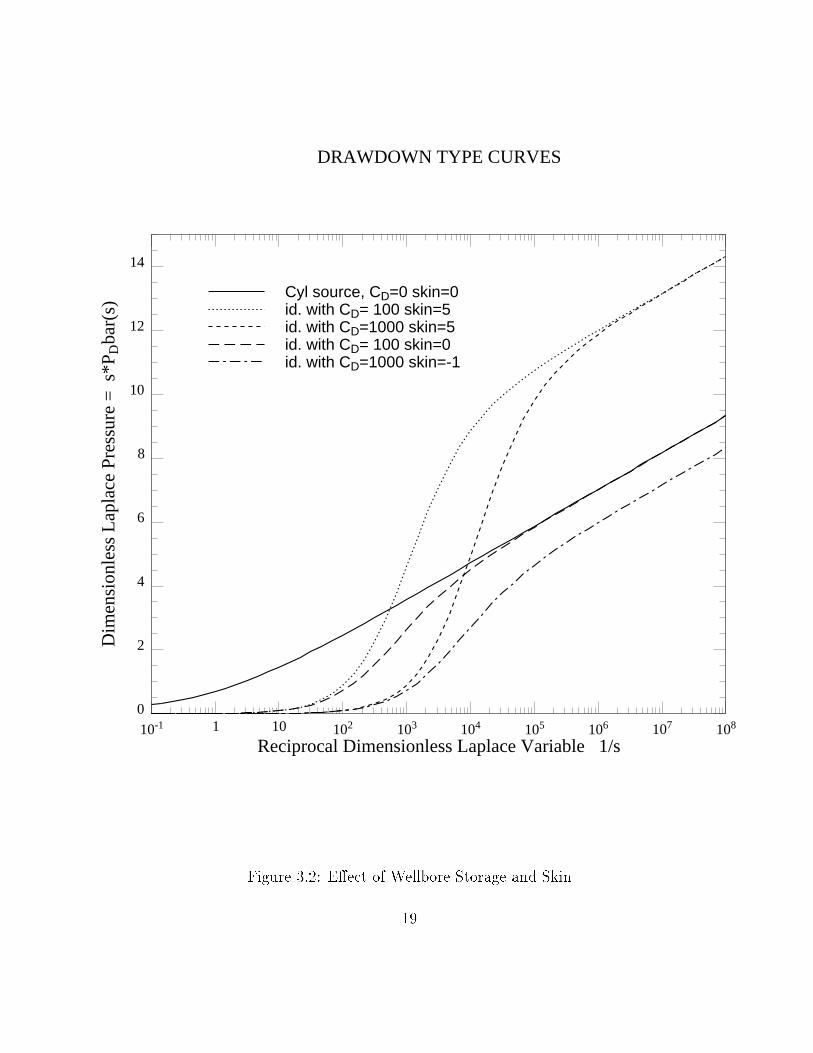
Laplace variable 1s, as is shown in Figure 3.2. It is easy to see that when
wellbore storage is present, the actual reservoir response is delayed, and that
the presence of skin adds a dimensionless pressure drop which increases with
the sandface owrate, and stabilizes at the value of the skin factor.
A log-log plot can be used to shift the data horizontally and vertically
until a good match is achieved. The Bourdet and al. [17] derivative type
curves are the most useful, because the derivative is very characteristic, since
it is located, thanks to its low value, in a part of the log-log plot where the
resolution is high. What is good for real pressure is also good for Laplace
pressure, and all we have to do is take the derivative Laplace quantities
equivalent to those in real space and to plot them in a similar way. This
17

allows us to display a set of type curves in log-log scale as well, as shown
in Figure 3.3. We plotted the Bourdet et al. type curve just below it to
emphasize the similarity in behavior. These type curves are valid only for
an in�nite acting, homogeneous reservoir (with the usual assumptions that
simplify the di�usivity equation). Since there is radial ow under these
circumstances, the two parameters CD and skin (which we will note S) can
be merged into CDe2S, which is an approximation we already know from
real space, and which is valid as soon as the Kernel Function has a semilog
behavior (with a 1/2 slope), which is the case for the time range tD > 30
. The only problem can be with very low values of CDe2S, where it becomes
necessary to index the curves with both parameters CD and S separately,
however this is quite rare in practice. This problem exists in real space as
well, as it is attribuable to the physics of the problem.
The log-derivative with respect to 1=s can be computed as follows:
d(spD(s))
dln(1=s)= �s d(spD(s))
ds(3:19)
This derivative is smoother than in real space, because the Laplace pres-
sure is still de�ned with an integral, and therefore the transitions in Laplace
space are less abrupt than in real space. In this regard, the Laplace pres-
sure derivative type curves are similar to the integral pressure type curves
described by Reynolds and Blasingame.
@2pD
@r2D
+1
rD
@pD
@rD=
@pD
@tD(3.20)
@2pD
@r2D
+1
rD
@pD
@rD= s pD(s) � pD(tD = 0+) (3.21)
The arguments in favor of the Laplace space approach are that even
when the real data are very noisy, the Laplace pressure and its derivative are
still smooth, which makes it a very e�cient diagnostic tool. Moreover, the
better knowledge of the reservoir solutions in Laplace space and the fact that
the treatment of owrate variations is simpli�ed, as shown in the following
chapters, make the method more broadly useful in practice.
18
0
2
4
6
8
10
12
14
Dim
ensi
onle
ss L
apla
ce P
ress
ure
= s
*PD
bar(
s)
10-1 1 10 102 103 104 105 106 107 108
Reciprocal Dimensionless Laplace Variable 1/s
Cyl source, CD=0 skin=0 id. with CD= 100 skin=5 id. with CD=1000 skin=5 id. with CD= 100 skin=0 id. with CD=1000 skin=-1
DRAWDOWN TYPE CURVES
Figure 3.2: E�ect of Wellbore Storage and Skin
19
One other useful advantage of Laplace space is that double porosity be-
havior can be taken into account very easily by replacing s by:
u = s f(s) = s!(1� !)s+ �
(1� !)s+ �(3:22)
in the argument of the Bessel functions (Warren and Root, Ref. [18]).
This holds for pseudosteady state interporosity ow, while for transient in-
terporosity ow, the model suggested by deSwaan-O (Ref. [19]) can be used:
s f (s) = s ( 1 +
s�0!0
3stanh(
s3!0s
�0)) (3:23)
The de�nitions of �0 and !0 are given by:
!0 =(�cth)m
(�cth)f(3:24)
and
�0 =12L2
h2m
(kh)m
(kh)f(3:25)
In Eqs. 3.24 and 3.25, hm and hf are the thickness of the individual matrix
and fracture elements, respectively. The de�nition of the dimensionless time
for this model is given by:
tD =kft
(�ct)f�L2(3:26)
Type curves for pseudo steady state interporosity ow are shown in Fig-
ure 3.4. The �rst plot, which is in semilog scale, shows the Kernel function
of the reservoir, which is the response if neither wellbore storage nor skin
were present, and if the sandface owrate had been a unit step function. For
the second plot, which is in log-log scale, the more conventional case of a
wellbore pressure including skin and wellbore storage is shown. The charac-
teristic e�ects of ! and � are the same as in real space, which is predictable
considering the poperties of the Laplace pressure.
20

Laplace Pressure Drawdown Type Curves
10-1
1
10
102
PD
(tD
)
10-1 1 10 102 103 104 105
tD / CD
CDe2S = 1030,1012,106,103, 10, 3
10-1
1
10
102
sP D
bar(
s)
10-1 1 10 102 103 104 105
1 / ( s *CD )
CDe2S = 1030,1012,106,103, 10, 3
Figure 3.3: Derivative Type Curves
21

Double Porosity Behavior during Drawdown
0.1 1 10 100 1000 10000 100000 1000000
1 / ( s * cd )
0.1
1
10
100
s*P
dbar
(s)
f
f
f
f
f
f
f
f
f
f
f
f
f
f
f
f
f
f
f
f
f
f
f
f
f
f
f
f
f
f
f
f
f
f
f
ff
ff
ff
ff
ff
ff
ff
ff
f f f f f f f f f f f f f f f f f f f f f f f f f f f f
f
f
f
f
f
f
f
f
f
f
f
f
f
f
f
f
f
f
f
f
f
f
ff f
f
f
f
f
f
f
f
f
f
f
f
f
f
f
f
f
f
f
f
f
f
f
f
ff
ff
ff
f f f f f f f f f f f f f f f f f f f f f f f f f f
f Cyl source cd=500 Skin=5, homogeneousid., double porosity w=0.1 lambda=1E-6id., double porosity w=00.1 lambda=1E-6id., double porosity w=00.1 lambda=1E-7
0.0001 0.01 1. 100 10000 1000000 1e8
Reciprocal Dimensionless Laplace Variable 1 / s
0
2
4
6
8
10
12
Lap
lace
Ker
nel F
unct
ion
= s
*Kba
r(s)
Cyl source, homogeneous reservoirid. with w=0.01 lambda=1E-6id. with w=0.1 lambda=1E-6id. with w=0.01 lambda=1E-4id. with w=0.1 lambda=1E-4
Figure 3.4: E�ect of Storativity Contrast ! and Transfer Coe�cient �
22

Figure 3.5, shows the e�ect of partial penetration on the Kernel function.
The plots do not include the e�ect of wellbore storage and skin due to damage
at the wellbore. The �rst plot is in semilog scale, therefore the additional
partial penetration skin is obvious. The values of this partial penetration
skin are the same as if conventional real space plots had been used. In the
second plot, which is log-log scale, di�erent ow regimes are visible. At
early time (that means at small 1=s), the �rst radial ow is visible, with a
Laplace pressure drop inversely proportionnal to the completion ratio. At
middle times, we expect a -1/2 slope of the log-derivative in real space,
but in Laplace space, since the transition is stretched, this spherical ow
behavior is visible only for extremely small completion ratios (hw=h < 5%).
The Kernel function has been computed for completion in the middle of the
layer (zw = h=2), for a homogeneous reservoir (u = s), using the following
expression:
sK(s) = K0(rDpu) +
4
�
h
hw
1Xn=1
(1
nK0(rD
su+
n2�2
h2D
) (3.27)
sin n�hw
2hcos n�
zw
hcos n�
z
h) (3.28)
Figure 3.6 shows the pressure drop in a well with wellbore storage and
skin in a reservoir with a closed outer boundary. The linear pressure drop
with respect to time gives a unit slope on a log-log plot, in Laplace space as
well as in real space. The Kernel fuction has been computed with:
sK =K1(reD
ps)I0(rD
ps) + I1(reD
ps)K0(rD
ps)p
s(I1(reDps)K1(
ps)� I1(
ps)K1(reD
ps))
(3:29)
If reD � 1, this can be approximated as:
sK = K0(rDps) +
K1(reDps)I0(rD
ps)
I1(reDps)
(3:30)
23

Partial Penetration At The Wellbore
0.01 0.1 1. 10 100 1000 10000 100000 1000000
1 / s
0.001
0.01
0.1
1
10
s *
Kba
r(s)
Line source, fully penetratingid., partial penetr., h/rw=200 hw/h=0.2id., partial penetr., h/rw=100 hw/h=0.2id., partial penetr., h/rw=50 hw/h=0.2id., partial penetr., h/rw=100 hw/h=0.05
0.01 0.1 1. 10 100 1000 10000 100000 1000000
1 / s
0
5
10
15
20
25
s *
Kba
r(s)
Line source, fully penetratingid., partial penetrating, h/rw=200 hw/h=0.2id., partial penetrating, h/rw=100 hw/h=0.2id., partial penetrating, h/rw=50 hw/h=0.2id., partial penetrating, h/rw=100 hw/h=0.5
Figure 3.5: E�ect Of Completion Ratio hw=h On The Kernel Function
24

Closed Outer Boundary For Homogeneous Reservoir
0.1 1 10 100 1000 10000 100000 1000000 1e7
1 / ( s * cd )
0.1
1
10
100
1000
s*P
dbar
(s)
and
- s
* d(
s*Pd
bar(
s))
/ ds
Cyl source with cd=500 skin=5 red=1000Derivativeidem , infinite acting wellDerivative
1 10 100 1000 10000 100000 1000000 1e7 1e8
1 / s
0
5
10
15
20
25
30
s*P
dbar
(s)
Cyl source with cd=500 skin=5 red=1000idem , infinite acting well
Figure 3.6: Linear Late Time Behavior For Bounded Reservoir
25
3.3 Treatment Of Wellhead Flowrate Varia-
tion
The previous section demonstrated that it was possible to generate charac-
teristic type curves in Laplace space for any kind of problem using the solu-
tions already published in the literature. However this is already possible in
real space as well, although usually more time consuming, especially when
in�nite series have to be used for the computations. This section shows treat-
ments for which the Laplace space approach brings substantial advantanges
in comparison to the real space approach, using the background described in
Section 2.2.
There are di�erent kinds of deconvolution, depending on the physical ori-
gin of the owrate variation and of the data available. If downhole owrate
measurements are available, wellbore storage deconvolution can be performed,
as explained in Section 3.5. However in practice, there are other causes of
owrate variation than just wellbore unloading, and the most common is the
fact that even at the wellhead, it is di�cult to maintain the owrate constant
during the whole test. This can be due to change of the chokes, or by a slow
cleaning-up of the well, or because the pump gets too weak when the pressure
drop increases, or when light oils are evaporating, or many other reasons. The
deconvolution treatment, namely dividing by the Laplace wellhead owrate,
is straightforward and stable:
s pwDc=
s pwD(s)
s qwhD(s)(3:31)
pwDcis the dimensionless wellbore pressure that we would have measured
if the owrate had been constant at the wellhead. It therefore includes well-
bore storage and skin e�ect, since the boundary condition (qwhD = 1) is
applied downstream of the wellbore. The advantage of this treatment is that
the whole rate history can be used for the match, and not only the last time
range where the owrate is (supposed to be) stable. Thus, more information
can be taken into account.
For the theoretical case where the owrate is a step variation, the treat-
ment is very simple, as it is in real space.
26

If tD < 0 qwhD = 0 (3.32)
0 < tD < tD1 qwhD = q1 (3.33)
tD1 < tD < tDmax qwhD = q2 (3.34)
Then s qwhD = q1 + (q2 � q1) e�stD1 (3.35)
This treatment is very e�cient and does not give any problems whatso-
ever, but can be made in real space as well. The advantage of the Laplace
approach appears when the wellhead owrate is not a succession of perfect
step functions. The Laplace transform has to be taken numerically, and the
deconvolution gives good results if the owrate measurements are accurate
enough.
As an example, consider the owrate history displayed in Figure 3.7. The
pressure data have been generated with 0.2 % random noise, using the su-
perposition of the owrate data. The model is a fully completed wellbore in
a homogeneous reservoir (k = 150mD; h = 35ft), with a wellbore storage
coe�cient of C = 0:006bbl=psi, and a skin of S = 1:3. In addition, there is a
sealing linear boundary, at a distance of 340ft from the wellbore.
A �rst match has been performed assuming that the owrate was con-
stant, which is certainly not true for the �rst 3 minutes. The production
time is 72 hours. The match (�rst plot of Figure 3.8) gives erroneous results
for all the parameters if the whole time range is considered, even though the
owrate looked almost perfect on the Cartesian plot. This emphasizes the
importance of the early time data.
The second step took into account the variable wellhead owrate. We
took the Laplace transform of these data, and deconvolved the pressure data
using Eq. 3.31. The results are plotted in Laplace space, using the appropri-
ate variables sf pw(sf) vs. 1=sf . The third plot of Figure 3.8 displays the
deconvolved pressure and the match, after coming back to real space using
Stehfest's algorithm. It can be seen that even though the data were some-
what noisy, the deconvolution is stable except for the �rst couple of points,
and that it gives very good results for the parameter estimation.
27

Flowrate at the Wellhead
0.001 0.01 0.1 1 10
time t (hr)
0
500
1000
1500
2000
2500
3000
3500
4000
flo
wra
te
(bbl
/hr)
c
cccccc
c
c
c
c
c
c
c
c
c
c
c
c
c
c
c
c
c
c
c
cc
c
c
c
c
cc
cc
c cc
c c c c c c c c c cccc c c c c c c c c c c c c c c c c c c c c c c c c c c c c c c c c c c c c c c c c c c c c c c c c c
c flowrate used to generate pressure
0 10 20 30 40 50 60 70
time t (hr)
0
500
1000
1500
2000
2500
3000
3500
4000
flo
wra
te
(bbl
/hr)
c
cccccc
c
c
c
c
c
c
c
c
c
c
c
c
c
c
c
c
c
c
c
cc
c
c
c
c
cc
cc
ccc
ccccccccccccccccccccccccccccccccccccccc c c c c c c c c c c c c c c c c c c c c c c c
c flowrate used to generate pressure
Figure 3.7: Cartesian and Semilog Plot Of Flowrate History
This highlights the importance of wellhead owrate measurements, and
demonstrates that drawdown data can be analysed successfully when qwh is
measured. The same is true, of course, if the measured owrate is a downhole
owrate. This even shortens the storage transition period, and gives the
best interpretation results. The only problem is that they are sometimes
di�cult to perform in practice, but recent improvements in downhole owrate
mesurement devices seem to be very encouraging in this regard. The �eld
example in the Appendix shows a succesful application of this technique. It
is not necessary to perform a costly buildup if the owrate can be measured.
28

Figure 3.8: Deconvolution Of Wellhead Flowrate Variation
29

3.4 Buildup With No Measurement Prior
To Shut-In
This section deals with an often encountered practical problem, which is that
no measurements were made during the production time, and that only the
pressure transient during the buildup was recorded. The procedure described
here is equivalent to rewriting the buildup pressure �le as a function of Agar-
wal's equivalent time (see Eq. 3.11, or Ref. [20]).
We know that buildup data do not behave like drawdown data, and there-
fore we cannot treat them in exactly the same way, especially when the
duration of the test is not negligeable in comparison with the preceding pro-
duction time. In real time, the solution is to use the \Horner" time, de�ned
as:
tH =tp + �t
�t(3:36)
If we denote as pBU(�t) the buildup pressure with measurements starting
at shut-in time (�t = 0), we have in real space:
pBU(�t) = pDD(�t) � ( pDD(tp +�t) � pDD(tp) ) (3:37)
If the initial drawdown has reached semilog behavior during the produc-
tion time ( t < tp, with usually b = 1=2 ), we can derive:
pDD(tp +�t) = a + b ln(tp + �t) (3.38)
! dpBU
dln(tH)= �dpDD(�t)
dln(�t)� �t
tp(�t p0
DD(�t) � b ) (3.39)
Therefore, as soon as pDD(�t) reaches semilog behavior, the slope on the
Horner plot is the same as the slope we would have had on a traditional plot
for a drawdown test. The approximation is all the better if tp is large.
We followed the same philosophy to �nd a Laplace variable which enables
us to treat a builup test as a drawdown. Our new time variable will be �t
in the Laplace transform, and we de�ne, with dimensionless variables:
30
pBUD(s) =Z1
�tD=0e�s�tD pBUD(�tD) d�tD (3:40)
Since we take the integral over the whole tD range, the approximations
must be valid over this whole range, and the only assumption we are making
is that of Eq. 3.39. We �nd the same truncated integral that we found in
Section 2.4, which yields an exponential integral:
s pBUD(s) = s pDDD(s) � b estpD E1(stpD) (3:41)
We have found a \Horner-like Laplace variable", which we call here sBU ,
which has the required property: a spBUD(s) vs. sBU plot has exactly the
same shape as (it is identical to) a spDDD(s) vs. s plot. To do so we used
the asymptotic behavior of the exponential integral, which can be found,
although not over the whole x range at once, in Abramowitz's Handbook of
Mathematical Functions (Ref. [21]):
� ln(x)� < exE1(x) <1
x(3:42)
For small x, the left-hand approximation is valid, and can be rewritten
as ln(1 + e� =x), and when x ! 1, the 1=x expression can be used, which
we will rewrite as well as ln(1 + 1=x). This can be summarized saying that:
exE1(x) ' ln(1 +A(x)
x) (3:43)
with A(x) continuously increasing from:
limx!0A(x) = e� ' 0:5614594835 (3:44)
to limx!1A(x) = 1 (3:45)
We de�ne the dimensionless buildup Laplace variable sBU as:
sBU = s +A(s � tpD)
tpD(3:46)
The full dimension buildup Laplace variable sBUf is similarly:
sBUf = sf +A(sf � tp)
tp(3:47)
31

We derived a homographic approximation equating the two expressions
in Eq. 3.43 for di�erent values of x. Eq. 3.43 can then be used to compute the
exponential integral for the whole positive x range (even for other purposes).
The simplest is:
A(x) =x + 1:035e�
x + 1:035(3:48)
We prefer to work with a re�ned expression, which has a better �t:
A(x) =x2 + 1:60718 x + 0:20025
x2 + 2:0908 x + 0:35181(3:49)
Our buildup Laplace variable is therefore:
sBU = s +1
tpd
(stpd)2 + 1:60718 (stpd) + 0:20025
(stpd)2 + 2:0908 (stpd) + 0:35181(3:50)
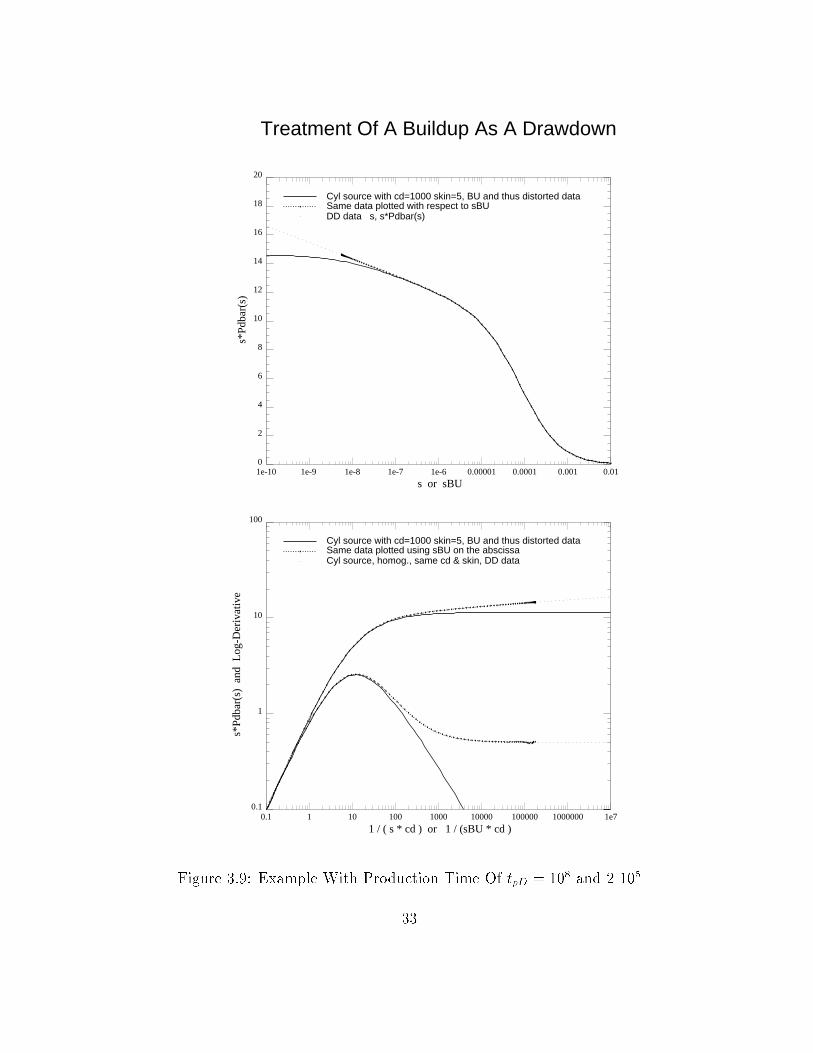
We have plotted the results on Fig. 3.9. As in real space Horner plots,
even though plotting spD(s) with respect to sBU can distort the data when
the assumptions to the treatment are not exact (no real semilog behavior),
this is still an excellent diagnostic tool.
We investigated the case where there was only one producing time before
the drawdown. In the case of a more complex owrate history before the
beginning of the pressure measurements, it is easier to use Agarwal's equiv-
alent time and subsequently to take the Laplace transform of the pw vs. teq�le, than to try to generalize this result.
As a conclusion to this section, we have found a Laplace variable which
is exactly equivalent to the Horner time in real space. We need the same
assumptions as in real space (see Eq. 3.39) if we want to have a graph without
distortion. The pressure buildup is all the bigger if the previous production
time was long, so this appears as a constraint on our variable, as seen in
Fig. 3.9.
�t + tp
�t> 1 (3.51)
is similar to sBU >e�
tpD(3.52)
32
Treatment Of A Buildup As A Drawdown
0.1 1 10 100 1000 10000 100000 1000000 1e7
1 / ( s * cd ) or 1 / (sBU * cd )
0.1
1
10
100
s*P
dbar
(s)
and
Log
-Der
ivat
ive
e
e
e
e
e
e
e
e
e
e
e
e
e
e
e
e
e
e
e
e
e
e
e
e
e
e
eeeeeeeee e e e e e e e e e e e e e e e e e e e e e e e e e e e e e e e eee
eeeeeeeeeeeeeeeeeeeeeeeeeeeeeeeeeeeeeeeeeeeeeee
e
e
e
e
e
e
e
e
e
e
e
e
e
e
e
e
e
e
e
eeee e e e
eee
e
e
e
e
e
e
e
e
e
e
e
eeeeeeee e e e e e e e e e e e e e e e e e e eeeeeeeeeeeeeeeee
eee
e
e
e
e
e
e
e
e
e
e
e
e
e
e
e
e
e
e
e
e
e
e
e
e
e
e
e
e
e
e
e
ee
ee
ee
ee
ee
ee
ee
e e e e e e e e e e e e e e e e e e e e e e e e e e e e e e e e e e e e e e e e e
e
e
e
e
e
e
e
e
e
e
e
e
e
e
e
e
e
e e e
e
e
e
e
e
e
e
e
e
e
e
e
e
e
e
e
e
e
e
e
e
e
e
ee
ee
ee e e e e e e e e e e e e e e e e e e e e e e e e e e e e e e e e e e e e e
e
e
Cyl source with cd=1000 skin=5, BU and thus distorted dataSame data plotted using sBU on the abscissaCyl source, homog., same cd & skin, DD data
1e-10 1e-9 1e-8 1e-7 1e-6 0.00001 0.0001 0.001 0.01
s or sBU
0
2
4
6
8
10
12
14
16
18
20
s*P
dbar
(s)
eeeeeeeeeeeeeeeeeeeeeeeeeeeeeeeeeeeeeeeeeeeeeeeeee e e eeeeeeeeeeeeeeeeeeeeeeeeeee
e
e
e
e
e
e
e
e
e
e
e
e
e
e
e
e
e
e
e
e
e
e
e
e
e
eeeeee e e e e e e e
e
e
e
e
e
e
e
e
e
e
e
e
e
e
e
e
e
e
e
e
e
e
e
e
e
e
e
e
e
e
e
e
e
e
e
e
e
e
e
e
e
e
e
e
e
e
e
e
e
e
e
e
e
e
e
e
e
e
e
e
e
e
e
e
e
e
e
e
e
e
e
e
e
e
e
e
e
e
e
e
e
e
e
e
ee
ee
ee e
e
e
Cyl source with cd=1000 skin=5, BU and thus distorted dataSame data plotted with respect to sBUDD data s, s*Pdbar(s)
Figure 3.9: Example With Production Time Of tpD = 108 and 2 105
33

3.5 Numerically StableWellbore Storage Re-
moval
Since the e�ect of wellbore storage is to delay the owrate impulse on the
reservoir, removing the e�ect is a deconvolution process.
A lot of di�erent deconvolution algorithms already exist, either using di-
rect real space deconvolution, or curve-�tting approximations. The drawback
of the former is that they are generally recursive, and therefore add up errors
occuring in the �rst steps of the computation. The disadvantage of curve-
�tting is that it is an approximation, and needs a lot of computation prior to
deconvolution to �nd the best coe�cients of each function. A way to avoid
this problem is to constrain the deconvolved pressure to stabilize it, but this
requires additional computation time as well.
The advantage of our Laplace space approach is that it does not have this
stability problem due to recursivity, because the Laplace transform takes the
whole time range into account. The only stability problem we encountered
was at early times, for wellbore storage deconvolution. This can be handled
by removing the wellbore storage only partially, as will be shown in this
section. We must be aware of the fact that when the formulas of Section 2.2
are used with no downhole owrate measurements, we have to estimate the
sandface owrate as:
s qsfD(s) = 1 � CDs
2pwD(s) (3:53)
This formula looks interesting, because we do not need to know kh to
compute it, since �p = �t=�C . However using this formula, deconvolution is
unstable numerically. This means that the slightest noise, or a small inaccu-
racy of our C estimate, or the fact that the physical wellbore storage is not
constant, make this treatment impossible in practice. This is understand-
able because the time derivative of the cylindrical source function tends to
in�nity at early time, and therefore creates a singularity in the convolution
integral. This is why if deconvolution has to be performed, the owrate used
34
should not be the sandface owrate, but the owrate just above the perfo-
rations, which we will call qm, because this is the owrate measured when a
bottomhole owmeter is installed. This has the advantage that there is the
small remaining storage of the rathole, or of the small volume of the wellbore
under the owmeter, which will stabilize the deconvolution. We will call Cr
this residual storage, and pwc the deconvolved pressure . pwc is the measured
pressure drop if the bottomhole owrate is a unit step:
qmD = 1 if t > 0 (3:54)
Actually, with this assumption, the sandface owrate at early times is
smaller than unity, and the following mass balances can be written, assuming
constant wellbore storage:
qsfD = qwhD � CD
dpwD
dtD(3.55)
qmD = qwhD � (C � Cr)DdpwD
dtD(3.56)
Since the di�usivity equation is linear, the pressure drops remain propor-
tional to the owrate, and thus:
s pwD(s) = s qmD(s) � s pwDc(s) (3:57)
This relation is exact, even if the wellbore storage is changing or if pw was
measured with a non-step wellhead owrate. This shows how much informa-
tion bottom-hole owrate measurements contain. In the simpler case where
pw corresponds to a constant wellhead owrate, the algebra to deconvolve
the pressure without owrate measurements is the following:
s pwDc(s) =s pwD(s)
1 � (C � Cr)D s2 pwD(s)(3:58)
This procedure has been tested on an example where a large wellbore
storage was hiding the early time behavior of the test, and deconvolution
removed the ambiguity by displaying an early time double porosity behavior.
This example is a 96 hour drawdown test, with simulated pressure data, to
which we have added 0.2 % noise. The model used was a reservoir with
pseudo-steady state double porosity behavior (! = 0:05 and � = 2 10�7),
35

with an impermeable linear boundary at a distance of rbdry = 300ft to the
wellbore. The other parameter values are: k = 200mD; S = 1:5, and
C = 0:1bbl=psi. The wellhead owrate was constant q = 2500bbl=day. For
the sake of completeness, the other parameters were: � = 0:2; � = 1cP; B =
1:2; h = 15ft; ct = 8 10�6=psi; and rw = 0:3ft.
We matched these pw(t) vs. t data using a simple in�nite-acting radial
ow model, with nonlinear regression (also known as automated type curve
matching), and we obtained the match of the �rst plot of Fig. 3.10. The
con�dence intervals were quite low, but the results were not correct. This
misinterpretation is due to a wrong model choice, and it is impossible to per-
form the proper model identi�cation without deconvolving (or having other
information).
To deconvolve these data, we needed measurements of the downhole
owrate. The owrate above the perforations was computed using Eq. 3.56,
with a rathole storage of Cr = 1:5% of C. We added 2 % noise to these qmdata for the �rst 6 minutes, and then 0.5 % noise until the end of the test.
We performed the devonvolution using the same algorithm as in section 3.3.
After deconvolution, the early time behavior is much more visible because
the huge wellbore storage is removed to 98.5 %, and it is clearly evident on a
log-log plot of pwc that there is a double porosity behavior for the reservoir,
and that there must be a boundary e�ect after 2 to 3 hours. We then per-
formed the matching on the deconvolved data using the exact model. This
is displayed in the second plot of Fig. 3.10. It can be seen that this interpre-
tation gives much better results than the �rst one. Nevertheless, the skin is
still quite poorly determined, as is rbdry. ! and � are poorly determined as
well, but this is nearly always the case.
36

Deconvolution With Noisy Flowrate Data
Figure 3.10: Matching With Wrong Model, Then Deconvolution, Then
Matching With Proper Model
37
The imprecision on the value of the skin is understandable since we know
that the skin is mostly determined by the wellbore storage transition. If
we work with deconvolved data, the range of the pressure response is much
smaller (we start with a bigger pressure drop) than for conventional data.
Nonetheless, deconvolution has allowed us to �nd the right model.
It was known in advance that it is better to perform matching on the
original variable rate data, since information is lost during the deconvolution
process. So, using the deconvolved data only as a means to recognize the
reservoir model, we then went back to the pw(t) vs. t data, and performed
the parameter estimation using the proper double porosity, impermeable lin-
ear boundary model. The results are summarized on the last plot of Fig. 3.10,
and it can be seen that this matching gives better results than with the de-
convolved data (second plot), again except for ! and �.
If we generalize these results, we can say that deconvolution allows us to
perform a good model identi�cation, and that the �nal match is the most
e�ective on non-deconvolved, traditional pw(t) vs. t data. This can be ex-
plained by the fact that if our impulse q is more complicated, it will give us
more information on the reservoir response pw.
As a conclusion to this section, wellbore storage deconvolution should
never be performed using the whole storage, but must leave a residual stor-
age to stabilize the treatment. If good downhole measurements are available,
deconvolution can be applied to perform model recognition, and if the data
are very good, it even allows parameter estimation on the deconvolved pres-
sure. If the owrate data are very noisy so that the computation of the
deconvolved pressure is impossible in real space, we can still examine the
deconvolved pressure in Laplace space, which is more stable, and still recog-
nizable. For this analysis, the type curves in Laplace space can be used to
recognize the shapes.
Therefore, as soon as the owrate, or in a less favorable situation the
storage, are measured with a satisfying accuracy, model identi�cation can be
performed using wellbore storage removal in Laplace space.
38
3.6 Pressure Dependant Wellbore Storage
In the previous section, the wellbore storage was assumed constant in time.
However we know that this is only a coarse assumption, since the compress-
ibility of the uids in the annulus is a function of pressure and tempera-
ture. Therefore, if a well test has a big pressure drop, the absolute pressure
pw = pw0 + �pw becomes important. We made the assumption that the
compressibility of the uids, and thus the wellbore storage as well, was in-
versely proportionnal to the absolute pressure. With dimensionless variables,
we denote in this section:
pwD = pwD0 + �pwD (3.59)
CD = CD0
pwD0
pwD(3.60)
Let us assume that we are using the results of the last section, and that
we only want to remove part of the wellbore storage, for example � = 90%.
This means C �Cr = �C. The owrate conservation equation still holds as:
qmD = 1 � � CD
dpwD
dtD(3:61)
The resulting Laplace owrate can be computed as:
s qmD(s) = 1 � � CD0 pwD0
Z1
0e�stD
dpwD(tD)
pwD(tD)dtDdtD (3.62)
= 1 � � CD0 pwD0 Lfd ln(pwD(tD))
dtDg (3.63)
= 1 � � CD0 pwD0 fs ln(pwD(tD)) � ln(pwD0)g (3.64)
= 1 � � CD0 pwD0 s ln(�pwD + pwD0
pwD0
)(s) (3.65)
The deconvolved pressure drop (or increment) can then be computed as:
39

s �pwDc(s) =s �pwD(s)
s qmD(s)(3.66)
=s �pwD(s)
1 � � CD0 pwD0 s ln(�pwD+pwD0
pwD0)(s)
(3.67)
To our knowledge, this expression is new as well. It may look unusual,
but it can be used with dimensional quantities, and this treatment can thus
be performed with only an estimate of the initial wellbore storage C0, which
is easily accessible. The absolute pressure pw0 at the beginning of the test
can be measured as well as the pressure drop, and we can write:
sf �pwc(sf ) =sf �pw(sf)
sf qm(sf )(3.68)
=sf �pw(sf )
1 � � C0 pw0 sf ln(�pw+pw0
pw0)(sf )
(3.69)
Again, since we have the data and the algorithm to take the Laplace
transform, nothing hinders us to perform this treatment, except the fact
that we never did it before. We tested this approach on the example plotted
on Fig. 3.11, which is a builup test from Alaska. The long lasting storage
transition and the important pressure increment made this test interesting
for our purpose. After wellbore storage removal, we were able to recognize
a radial composite model, which is in accordance with the fact that gas has
been injected around this well and therefore created a higher mobility zone
at some distance.
40

Removal of a Variable Storage
0.001 0.01 0.1 1 10 100
Time [hr]
1
10
100
1000
10000
Pres
sure
[ps
i]
Treated dataLog-derivative
0.001 0.01 0.1 1 10 100
Time [hr]
1
10
100
1000
10000
Pres
sure
[ps
i]
Initial dataLog-derivative
Figure 3.11: Application to Real Field Data (Buildup)
41

3.7 Nonlinear Regression in Laplace Space
Much of the parameter estimation in well test analysis today is performed
with automated type-curve matching, which amounts to a nonlinear regres-
sion to minimize the di�erence between the data and the chosen model. This
�nal step of the analysis has to be done once a model is chosen, and we have
seen previously some additional tools to perform model recognition. In par-
ticular, removing the wellbore storage can unveil some early-time behavior
indicative of a particular well or reservoir model. Usually, if we denote as
ndp the number of (pressure) data points, and ~� = (k;C; S; :::) the variable
vector which contains permeability, storage, skin and any other parameter
de�ned in the model, the problem can be formalized as follows:
Min~� �ndp
i=1[ pmodel(ti; ~�) � pmeasured(ti) ]2 (3:70)
Most models are known in Laplace space ([2, 3]), and therefore each
computation of pmodel(t; ~�) requires the use of a numerical inverter ([4, 5]).
Typically with Stehfest's algorithm, the computation of one point in real
space requires 6 or 8 computations in Laplace space. This is all the more
time-consuming as these computations may be expensive if in�nite sums
occur. This problem is further aggravated if numerous iterations (up to 10
or 20) have to be performed before convergence. Based on the work showed in
this study, we thought that we could choose a range for the Laplace variable,
where the Laplace pressure would convey as much information as the real
pressure itself. Logically, we chose ndp points , with 1=sf i = ti; i = 1::ndp.
The regression was performed using a least-square problem as well:
Min~� �ndp
i=1[ sf i pmodel(sf i; ~�) � sf i pmeasured(sf i) ]2 (3:71)
Of course, the parameter vector ~� is exactly the same as in the previous
equation. The �rst term of the square bracket is easier to compute than
previously, since it is computed directly in Laplace space. The second term
requires the application of a Laplace transform algorithm to the measured
data, for example apl8 listed in the Appendix. The advantage is that this
42

second term has to be computed only once, and does not change any more
as ~� is updated during the regression.
A Gauss-Newton minimization was performed using this approach. The
data were taken from the example treated in Fig. 3.10. We did the regression
assuming a standard in�nite acting, storage and skin model. The real space
regression algorithm converged in 8 iterations. With the same starting point,
our Laplace space algorithm converged to the same solution (within 1 %) in
6 iterations. The search path is shown in Fig. 3.12. The main di�erence
is not the number of iterations, but the fact that the regression requires
less computations for each iteration. The fact that the objective function is
smoother in Laplace space is only of slight advantage here. It would have been
more important if the data had been noisier. For example, it would probably
still be possible to match on the derivative in Laplace space, whereas we
would have to match on the pressure itself in real space, if the data were
very noisy. Another advantage of the regression in Laplace space is of course
when the owrate is varying during the test. Typically, if a downhole owrate
qm is measured, the regression can be performed directly on:
sf �pw(sf ) = sf �pwc(sf ) � sf qm(sf ) (3.72)
In such a case, regression in real space on pw(t) would require either a te-
dious superposition of pwc(t) [10], or an inversion of Eq. 3.72 with Stehfest's
algorithm for example [4, 5]. If Laplace space has to be used on the data
anyway for deconvolution, and since we usually have to use it for the model,
it seems logical to use it for the regression as well.
43

-5 -4 -3 -2 -1 0 1 2
Skin S
60
80
100
120
140
Perm
eabi
lity
k
[m
d]
c
c
c
c
ccc
c
c
c
c
c
c
ccc
c
cregression in Laplace spaceregression in real space
Search Path During Regression
Figure 3.12: Nonlinear Regression in Laplace Space and Real Space
44

Chapter 4
Conclusion
The following �ndings were obtained from this study:
(1) The Laplace transform can be displayed in a characteristic, familiar
looking way if the variables sf pw(sf ) vs. 1=sf are chosen. These variables
have the same dimension as pw(t) vs. t.
(2) Taking these variables, or the equivalent dimensionless expressions
s pwD(s) vs. 1=s, it is possible to plot type curves in Laplace space with the
same log-derivative as in real space. These type curves are smoother than
in real space, but still characteristic enough to perform model identi�cation.
If implemented in an automated type curve matching procedure, they allow
the whole parameter estimation to be performed in Laplace space, since the
Laplace transform contains as much information as its original function in
real space.
(3) Although we need to know the behavior of the function (usually pw(t))
over the whole time range, we have seen that a linear interpolation at early
time and a power extrapolation at late time, with �rst and second derivative
information, are satisfactory for the computation of the Laplace transform.
We developed adequate algorithms for this purpose, and tested them succes-
fully on simulated as well as on actual �eld data.
45

(4) We have found a Laplace variable sBU which is similar to Horner
time, and allows us to treat buildup tests like a drawdown, even with no
measurements prior to shut-in. The assumptions we need are the same as for
the Horner variable, namely that the preceeding production time was long
enough to have reached a semilog behavior.
(5) Our Laplace space approach is the natural approach if deconvolution
has to be performed. In practice, if owrate measurements are available,
the model must be recognized using either real space or Laplace space type
curves, but always dividing the Laplace pressure by the Laplace owrate.
If the quality of the data is good enough, �nal match can be obtained on
the deconvolved data, but the best results are usually found matching the
measured pressure data taking into account the owrate history with super-
position.
(6) For wellbore storage deconvolution without owrate measurements,
which is the less favorable case, the same procedure can be applied, sim-
ply estimating the owrate from the storage and the pressure derivative. A
residual storage should be left to stabilize that treatment. The storage does
not need to be assumed constant for this treatment.
(7) Nonlinear regression can be performed in Laplace space, and this has
been done successfully. The regression is computationally more e�cient, by
at least a factor of six or eight, depending on the value of the Stehfest param-
eter. The Laplace space regression also o�ers advantages if the data are noisy.
This approach provides an entirely new way of examining and under-
standing well test results.
46

4.1 Nomenclature
b = semilog slope
ct = total compressibility, psi�1
C = wellbore storage constant, bbl/psi
f = time fuction
h = formation thickness, ft
k = permeability, md
n = number of available data points
p = pressure, psi
q = owrate, B/D
r = radius, ft
s = Laplace variable (dimensionless)
sf = fully dimensional Laplace variable, hr�1
S = damage skin
t = time, hr
� = oil viscosity, cp
� = dummy integration variable
� = system porosity
! = storativity contrast in �ssured reservoirs
� = transfer coe�cient in �ssured reservoirs
4.2 Subscripts and Superscripts
D = dimensionless
H = Horner time
c = constant rate = deconvolved
sf = sandface
wh = wellhead
m = measured or at the owmeter
r = residual
w = well, wellbore or perforated0 = time derivative of
f = Laplace transform of f
47

Bibliography
[1] van Everdingen, A.F. and Hurst, W.: \The Application of the
Laplace Transformation to Flow Problems in Reservoirs", Trans., AIME
(1949)186, 305-324.
[2] Ozkan, E. and Raghavan, R.: \Some New Solutions to Solve Problems
in Well Test Analysis: Part 1 - Analytical Considerations", SPE 18165,
1989.
[3] Ozkan, E. and Raghavan, R.: \Some New Solutions to Solve Problems
in Well Test Analysis: Part 2 -Computational Considerations and Ap-
plications", Nov. 1989.
[4] Crump, K.S.: \Numerical Inversion of Laplace Transforms Using a
Fourier Series Approximation", Journal of the ACM, Jan. 1976, Vol.
23, 89-96.
[5] Stehfest, H.: \Numerical Inversion of Laplace Transforms", Communi-
cation of the ACM, Jan. 1970, Vol. 13, No.1, 47-49.
[6] Rosa, A.J. and Horne, R.N.: \Automated Type-Curve Matching in Well
Test Analysis by Using Laplace Space Determination of Parameter Gra-
dients", paper 12131 presented at the 1983 SPE Annual Technical Con-
ference and Exhibition, San Francisco, Sept. 5-8.
[7] Kuchuk, F.J., Carter, R.G. and Ayestaran, L.: \Numerical Deconvolu-
tion of Wellbore Pressure and Flow Rate", SPE 13960, 1985.
[8] Kuchuk, F.J.: \Applications of Convolution and Deconvolution to Tran-
sient Well Tests", SPEFE, Dec. 1990.
48
[9] Chaumet, P., Pouille, J. and S�eguier, P.: \Application de la transforma-
tion de Laplace �a l'�etude des courbes de pression en r�egime transitoire",
Revue de l'Institut Fran�cais du P�etrole, Dec. 1962.
[10] Guillot, A.Y. and Horne, R.N.: \Using Simultaneous Downhole Flow
Rate and Pressure Measurements To Improve Analysis of Well Tests",
SPEFE, June 1986, 217-26.
[11] Romboutsos, A. and Stewart, G.: \A Direct Deconvolution or Convolu-
tion Algorithm for Well Test Analysis", paper SPE 18157 presented at
the 63rd SPE Annual Technical Conference and Exhibition, Houston,
TX, Oct. 2-5, 1988.
[12] Earlougher, R.C. Jr. and Kersch, K.M.: \Analysis of Short-Time Tran-
sient Test Data by Type-Curve Matching", JPT, July 1974, 793-800;
Trans., AIME, 257.
[13] Gringarten, A.C.: \Type-Curve Analysis: What It Can Do and Cannot
Do", paper SPE 16388, JPT, Jan. 1987, 11-13.
[14] Gringarten, A.C. et al.: \A Comparison Between Di�erent Skin and
Wellbore Storage Type-Curves for Early-Time Transient Analysis", pa-
per SPE 8205 presented at the 1979 SPE Annual Technical Conference
and Exhibition, Las Vegas, Sept. 23-26.
[15] Ramey, H.J., Jr. and Agarwal, R.G.: \Annulus Unloading Rates as
In uenced by Wellbore Storage and Skin E�ect", SPEJ, Oct. 1972, 453-
62.
[16] Ramey, H.J. Jr.: \Short-Time Well Test Data Interpretation in the Pres-
ence of Skin E�ect and Wellbore Storage", JPT, Jan. 1970, 97-104;
Trans., AIME, 257.
[17] Bourdet, D. et al: \A New Set of Type Curves Simpli�es Well Test
Analysis", World Oil, May 1983, 95-106.
[18] Warren, J.E. and Root, P.J.: \The Behavior of Naturally Fractured
Reservoirs", SPEJ, Sept. 1963, 245-255.
49
[19] deSwaan - 0, A.: \Analytical Solutions for Determining Naturally Frac-
tured Reservoir Properties by Well Testing", SPEJ, June 1960, 117-122.
[20] Agarwal, R.G.: \A New Method to Account for Producing TIme E�ects
When Drawdown Type Curves are Used to Analyse Pressure Buildup
and Other Test Data", paper SPE 9289 presented at the 55th SPE
Annual Technical Conference and Exhibition, Dallas, TX, Sept 21-24,
1980.
[21] Abramowitz, M. and Stegun, I.A.: \Handbook of Mathematical Func-
tions", Dover Publications, Inc., New York (1972)
[22] Meunier, D.F., Wittman. M.J. and Stewart, G.: \Interpretation of Pres-
sure Buildup Test Using In-Situ Measurement of After ow", JPT, Jan.
1985, 143-52.
50

Chapter 5
Appendix
5.1 Fortran Program
real*8 function flapl8(s,pd,td,ndp,pinitl)
c - written by Marcel Bourgeois, Nov 1991
c - takes the Laplace transform of a (p,t) file written as array
c - can be used for pressure or flowrate, dimensionless or not
c expin= exponential integral, DGAMIC= incomplete Gamma function
c
IMPLICIT real*8 (a-h, o-z)
dimension pd(400), td(400)
c - computation of last semilog slope on 0.1 or 0.2 log cycle
nstep = 2
if (nstep.eq.1) width=0.2
if (nstep.eq.2) width=0.1
if (nstep.eq.3) width=0.05
do 60 ii=ndp-1, 2, -1
if (dlog(td(ndp)/td(ii)).ge.width) then
i=ii
goto 62
endif
60 continue
62 do 65 kk=i-1, 1, -1
if (dlog(td(i)/td(kk)).ge.width) then
k=kk
goto 67
endif
65 continue
c ----- left log derivative -----
67 m = dlog(td(ndp)/td(i)) * pd(k)
& / ( dlog(td(i)/td(k)) * dlog(td(ndp)/td(k)) )
& + dlog( td(ndp)*td(ndp)/(td(i)*td(k)) ) * pd(ndp)
& / ( dlog(td(ndp)/td(i)) * dlog(td(ndp)/td(k)) )
& - dlog(td(ndp)/td(k)) * pd(i)
& / ( dlog(td(i)/td(k)) * dlog(td(ndp)/td(i)) )
c --
51

a = 2* pd(k) / ( dlog(td(i)/td(k)) * dlog(td(ndp)/td(k)) )
& - 2* pd(i) / ( dlog(td(ndp)/td(i)) * dlog(td(i)/td(k)) )
& + 2*pd(ndp) / ( dlog(td(ndp)/td(k)) * dlog(td(ndp)/td(i)) )
c
c - computation of Laplace transform with linear interpolation between
c - data points, and power extrapolation afterwards
c
f0 = (pd(1)-pinitl) / td(1)
sum= f0 * (1. - dexp(-s*td(1)) ) / (s*s)
do 1 i=1, ndp-1
fi = (pd(i+1)-pd(i)) / (td(i+1)-td(i))
sum = sum + fi * ( dexp(-s*td(i)) - dexp(-s*td(i+1)) ) / (s*s)
1 continue
c - a log-log extrapolation for the derivative for large t -----------
alpha= a / m
alpha1=alpha+1.d0
xn= s*td(ndp)
if ( (dabs(alpha).gt.(1.d-1)) .and. (xn.lt.50) ) goto 68
c - if the derivative is flat enough, the exponential integral is OK
sum= sum+ m * expin(xn) / s
flapl8 = sum
return
68 sum= sum + m / (alpha*s* xn**alpha)
& * ( DGAMIC(alpha1,xn) - xn**alpha *dexp(-xn) )
flapl8 = sum
return
end
5.2 Field Example
The algorithms had to be validated not only on simulated data, to which
noise had been added, but also on a di�cult �eld case. This third example,
called Well A, is a drawdown test on a partially penetrated well, in a for-
mation known to be mildly layered. A � 1,000-ft rathole is present below
the producing zones. The well was put on production with the expectation
that the production rate would stabilize at a constant rate of 15,000 B/D.
Within a 20-minute period, a signi�cant drop in the downhole pressure was
noticed, and the production had to be decreased to avoid two-phase ow in
the wellbore and formation (see owrate in Fig. 5.1), resulting in a decreas-
ing pressure drop after � 30 min. Additionnally, data acquisition was halted
after 7 hours of recording because of operational problems. This test is not
interpretable without taking into account the owrate history, and model
recognition cannot be performed without deconvolution. The following for-
52

mula was used:
sf �pwc(sf ) =sf �pw(sf )
sf qm(sf)(5.1)
Regression (storage and skin match) was still performed in real space. Fig. 5.2
shows the result of deconvolution both in Laplace space and in real space.
The hemispherical ow due to partial penetration is visible, as well as the
slight double porosity behavior due to the layers. The results can be com-
pared with those in Ref. [8]. The apl8 algorithm was used to take the
(forward) Laplace transform of both the pressure and owrate data, and
Stehfest algorithm was used (with n=4) to take the inverse Laplace trans-
form. The results are good enough to make the Laplace approach interesting
in practice for deconvolution problems.
0
2000
4000
6000
8000
10000
12000
14000
16000
18000
Flo
wra
te q
m (
ST
B/D
)
10-3 10-2 10-1 1 10time (hours)
Figure 5.1: Well A: measured downhole owrate (�eld data)
53
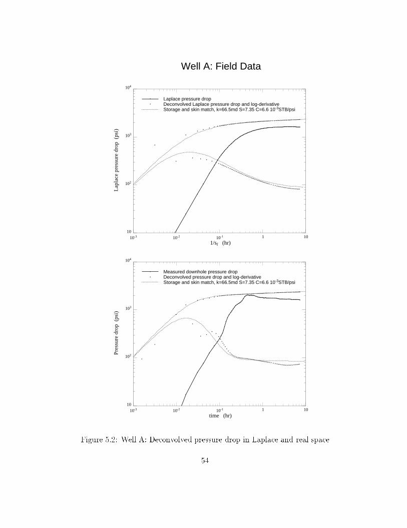
Well A: Field Data
10
102
103
104
Pre
ssur
e dr
op (
psi)
10-3 10-2 10-1 1 10
time (hr)
a
a
a
a
a
a
a
a
a
a
a
a
a
a
a
a
a
a
aaaaaa
a
aaaa a aaaa
a aaaaaaaaaaaa a a a a aa a a a aaa aaaa a aaaaaa
c
c
cc
cc
c c cccc cc c cc cc c c ccc cc c ccc c cccc c
cccccccccccc cc c c cc c c c ccc cccc c cccccc
c
c
c
c
c
c
c
c
c
c
c
c
c
c
c
ccccc c c ccc c c cccc ccccc cccccccccccc c c c c c cc c c c cc c ccc c ccccc
c
a
c
Measured downhole pressure dropDeconvolved pressure drop and log-derivativeStorage and skin match, k=66.5md S=7.35 C=6.6 10-3STB/psi
10
102
103
104
Lap
lace
pre
ssur
e dr
op (
psi)
10-3 10-2 10-1 1 10
1/sf (hr)
a
a
a
a
a
a
a
a
aaa
a
a
a
aaaaaaaaaaaaaa
a aaa
aaa a
aaaaaaa
aaaa aa a a aa a a a aaa aaaa a aaaaaa
c
c
c
c
cc
c c ccccc c c cc cc
c c ccc cc c ccc c c
ccc c cccccccccccc c
c c c cc c c c ccc cccc c cccccc
c
cc
cc
ccccccc
ccccc
ccccccc c
ccccc ccccc cccccccccccc c c
c c c cc c c c cc c ccc c cccccc
a
c
Laplace pressure dropDeconvolved Laplace pressure drop and log-derivativeStorage and skin match, k=66.5md S=7.35 C=6.6 10-3STB/psi
Figure 5.2: Well A: Deconvolved pressure drop in Laplace and real space
54