well test
TRANSCRIPT

ABOUT THE AUTHOR
Dr Mike Onyekonwu has a B.Sc. (First Class Honours) in
Petroleum Engineering from University of Ibadan, Nigeria. He
also has an MS and Ph.D. degrees in Petroleum Engineering from
Stanford University.
Dr Onyekonwu is a Senior Lecturer and former Head of Petroleum Engineering
Department, University of Port Harcourt. He is a member of University Senate. Dr
Onyekonwu is the founder and Managing Consultant of Laser Engineering Consultants,
Nigeria. Dr Onyekonwu worked for Shell Petroleum Development Company Nigeria
and Stanford University Petroleum Research Institute, California.
Dr Onyekonwu is a registered engineer and a member of different professional bodies.
He consults for Shell, Mobil, Elf, NNPC, Agip and other oil operating and service
companies. His area of specialization includes welltest analysis, reservoir simulation,
recovery methods and computer applications.
A very good and useful write-up which should be of help to a lot of young engineers
both at school and in industry.
Professor G. K. Falade.
Excellent material for teaching and practising engineers. Very practical (brings out many
very important information lost in the mathematics of transient pressure analysis) and
covers all important topics required by beginners and most engineers.
Professor Chi Ikoku
BHP BALANCE

ACHIEVED OBJECTIVE
BHP TEST
Field Operators
Test Analyst
Proposal
Writer
TABLE OF CONTENTS
PAGE
PREFACE ....................................................................................................................... ii
COURSE ADVERTISEMENT ........................................................................................ iii
1 INTRODUCTION ........................................................................................................... 1
1.1 Objectives of BHP Survey .. ........................................................................... 1
1.2 Uses of BHP Derived Information .................................................................. 1 1.3 Common Types of BHP Tests ........................................................................ 2
1.4 Ideal Conditions and Information Derived from Test ...................................... 3
1.5 Importance of Sticking to Ideal Condition for Test ......................................... 4 1.6 Uses of Information Derived from BHP Tests................................................. 6
1.7 Well Test Equipment ...................................................................................... 7
1.8 Electronic Gauges and Problems ................................................................... 11
1.9 Flowing Gradient/Buildup/Static Gradient(Fg/Bu/Sg) Survey ......................... 11 1.10 Flowing Gradient/Buildup/Static Gradient Survey Proposal ............................ 19
1.11 Useful Hints on Proper Testing of Wells......................................................... 23
1.12 Practical Hints ................................................................................................ 23
ACHIEVED OBJECTIVE

1.13 Gauge Quality Check Procedure ..................................................................... 27
1.14 Roles of Field Staff In BHP Survey ................................................................ 28 1.14.1 Roles of Production Staff ................................................................... 32
1.14.2 Roles of BHP Contractor Staff ........................................................... 33
2. BASIS OF ANALYZING BOTTOM HOLE PRESSURE TESTS ........................... 34
2.1 Flow Phases .................................................................................................. 34
2.2 Features of Different Phases .......................................................................... 35
3. ANALYSIS OF BOTTOM HOLE PRESSURE TESTS .......................................... 46
4. EFFECT OF CERTAIN FACTORS ON ANALYSIS OF SIMULATED DATA ..... 64
4.1 Analysis of Ideal BHP Data ........................................................................... 64
4.2 Effect of Gauge Accuracy and Datum Correction .......................................... 73
4.3 Effect of Noise .............................................................................................. 78 4.4 Effect of Gauge Sensitivity ............................................................................ 98
4.5 Effect of Rate Variation ................................................................................. 98
4.6 Effects of Leaks ............................................................................................ 112
4.7 Effect of Interference/Leak ............................................................................ 112
5. FIELD CASES ....................................................................................................... 117
5.1 Good Test ..................................................................................................... 117 5.2 Effect of Gauge Movement ........................................................................... 117
5.3 Effect of Gauges Off-Depth ........................................................................... 125
5.4 Effect of Reporting Wrong Rates ................................................................... 125 5.5 Effect of Ineffective Shut-in/Well not flowing before Shut-in ......................... 131
5.6 Effect of Leak ............................................................................................... 132
5.7 Effect of Gauge Oscillations/Sensitivity Problems ......................................... 135
5.8 Effect of Gas Phase Segregation .................................................................... 140 5.9 Effect of Liquid Interface Movement ............................................................. 144
5.10 Effect of Gaslift ............................................................................................. 144
5.11 Effect of Short Buildup or Flow Period .......................................................... 144
6. CLASS DISCUSSION ........................................................................................... 154
7. FLOWING AND STATIC GRADIENT SURVEYS ............................................... 165 8. SKIN FACTOR
8.1 What is Skin Factor ........................................................................................ 172
8.2 Causes of Skin ............................................................................................... 174 8.3 Classification of Pseudoskins ......................................................................... 174
8.4 Calculation of Pseudoskins ............................................................................. 176
8.5 Relationship Between Total Skin and Pseudoskins ......................................... 180
8.6 Pressure Change Due to Skin.......................................................................... 181 8.7 Relationship Between Skin and WIQI ............................................................ 181
Exercises ........................................................................................................ 182
APPENDIX A: TYPICAL PROPOSAL ........................................................................... 184
APPENDIX B: PROPOSAL WITH WRONG INSTRUCTION ....................................... 192
APPENDIX C: MISCELLANEOUS MATERIAL ............................................................
CHAPTER 4
ANALYSIS MODELS
Pressure – time data obtained from BHP tests are normally analyzed using mathematical
models. Figure 4.1 shows both the test and analysis principles.

Reservoir
k? s?
Pressure change
(Output)
Model
k, s, etc known
Same
Rate change
Rate change
(Input)
(Input) (Output)
Pressure change
Test Principle
Analysis Principle
Fig. 4.1: Test and Analysis Principles
The test principle involves perturbing the reservoir by applying some input (usually rate changes) and
measuring the resulting pressure. The analysis principle involves perturbing a mathematical model using
similar input applied to the reservoir and comparing the resulting pressure with actual pressures obtained during the test. The mathematical model is fine-tuned until the actual pressures obtained during the test
agree with pressures obtained with the mathematical model. It is then inferred that properties of the
mathematical model are similar to that of the reservoir. The uniqueness of the result is not the subject of
discussion now.
The choice of mathematical model is not arbitrary because pressure and pressure derivative obtained
during the test contain “signatures” that reveal the nature of the type of model to be used in the analysis.
Therefore understanding the models will help in relating to the reservoirs.
Each model used in test analysis may consists of 3 sub-models: well model, reservoir model and boundary
model. Options in the sub-models are shown in Table 4.1. Any well model can be used with any reservoir
model and any boundary model to make up the analysis model. However, in some cases, the mathematical models for the chosen sub-models may not be available or physically feasible. However, available choices
show that a number of mathematical models are available. The term reservoir model is used here to
represent the behaviour of the reservoir during transient state phase.
Table 4.1: Analysis Models
WELL MODELS RESERVOIR
MODELS
BOUNDARY
MODELS Wellbore storage and skin Homogeneous Closed
Changing Wellbore storage Single Fracture Constant Pressure
Limited entry well Double Porosity Fault
Horizontal well, etc. Composite Leaky Fault
Well on a Fracture
The boundary model will not be used if the late-time was not reached.
Although it is not possible to describe all analysis models, but the following models
deserve some mention: a. Wellbore storage and skin well in homogeneous reservoir
b. Wellbore storage and skin well on single vertical fracture
c. Wellbore storage and skin well in a double porosity reservoir.
Discussion on these follows:
4.1 Wellbore Storage and Skin Well in Homogeneous Reservoir. A homogeneous reservoir is one whose properties (permeability and porosity) are invariant in the direction
of flow. This is the most common model and many high permeability formations (eg. Niger Delta) are
homogenous. Typical profiles for a well with wellbore storage and skin in a homogenous reservoir are
shown in Fig 4.2.

Get figure from kappa book page B8-3 ?????
Fig. 4.2: Profiles from Well with Wellbore Storage and Skin in Homogenous Reservoir
Note that no boundary model was used because test ended during the infinite-acting radial flow (I. A.R.F)
phase.
Parameters that can be deduced with this model are as follows
Cs = wellbore storage constant
s = skin factor
k = permeability
4.2 Well on a Single Vertical Fracture
It is not unlikely that a well is located on a single vertical or horizontal fracture as shown in Fig 4.3. The
fracture which was caused by faulting or fracturing becomes a fast track for fluids getting to the wellbore.
?????????????? This figure is from welltest theory page 55 and 56
Fig 4.3: Fractured Wells.
Parameters that can be deduced with this model include the following:
xf = fracture half length
k = permeability
Cs = wellbore storage constant
s = skin factor
Three forms of this model depending on the flow in the fracture exist. They are as follows:
(a) Infinite conductivity fracture
(b) Finite conductivity fracture
(c) Uniform flux fracture
Gringarten et al (1974) published solutions for these models. Features of the models are discussed.
4.2.1 Infinite Conductivity Fracture
This represents the case where the fracture permeability, kf , is much greater than the permeability of the
matrix, k (kf >> k). The fracture is considered to have an infinite permeability and therefore there is no
pressure drop during flow in the fracture. The pressure profile in this case is shown in Fig 4.4.
???????????????????? take from kappa book
Fig 4.4: Well on a single vertical infinite conductivity fracture.
This reservoir goes through a linear flow, followed by a pseudo-radial flow before the boundary effect.
However, no pseudo-radial flow will appear if xf/xe = 1. This is shown in Fig 4.5.

Ask for this ????? Remove unnecessary spaces
Fig 4.5: Effect of xf/xe on Well on a Single Vertical Infinite Fracture

4.2.2 Uniform Flux Fracture
In this case, fluid enters the fracture at uniform flowrate per unit area of fracture face so that there is a pressure drop
in the fracture. Features of uniform flux fracture are similar to the infinite conductivity case shown in Figures 4.4
and 4.5.
4.2.3 Finite conductivity fracture
In this case, fluid flows within the fracture and there is a pressure drop along the length of the fracture. Features of
this case are shown in Fig 4.6.
Take figure from kappa page B9-9
Fig 4.6: Log – Log Graph of Data from Well with Finite Conductivity Fracture
4.3 Double Porosity Reservoir
The double porosity reservoir is simply a fissured (naturally fractured) reservoir and is shown in Fig 4.7.
?????????????? take from horne’s book
Fig 4.7: Fissured Reservoir
The main feature of this reservoir is that the pore space is divided into two distinct media: the matrix, with high storativity and low permeability, and the fissures with high permeability and low storativity. Flow between the
fissure and matrix can occur under pseudo – steady state on transient state. However, the former is more common.
In addition to fissured reservoirs, double-porosity models can also represent layered reservoirs in which one layer
has a permeability that is much higher than the other. This is shown in Fig 4.8. Fluid essentially reaches the
wellbore through the layer with higher permeability.

Fig 4.8: Layered Reservoir
Layered reservoirs are also modeled with double permeability model (Bourdet, 1985), but the features of double
permeability model are similar to the double porosity model.
Warren and Root (1963), de Swaan (1976), Bourdet and Gringarten (1980) and Gringarten (1984) published double
porosity solutions. Informations that may be deduced with the double porosity model are as follows:
k = permeability
s = skin factor
Cs = wellbore storage constant
= ratio of the storativity in the most permeable medium to that of the total reservoir
= Inter porosity flow coefficient
Some parameters in the equations are defined as follows:
km = permeability of matrix or least permeable layer
=
VC
VC + VC
t fissure (f)
t (f) t (m)
fissure matrix
= r k
kw2
m
f
k2 >> k1
k1
kf = permeability of fracture or most permeable layer
V = ratio of the total volume of one medium (matrix or fissure) to the bulk volume
= characteristics of the geometry of the interporosity flow.
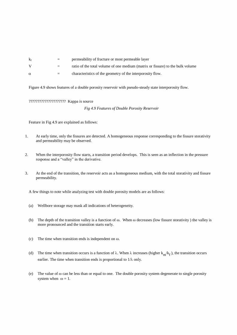
Figure 4.9 shows features of a double porosity reservoir with pseudo-steady state interporosity flow.
????????????????????? Kappa is source
Fig 4.9 Features of Double Porosity Reservoir
Feature in Fig 4.9 are explained as follows:
1. At early time, only the fissures are detected. A homogeneous response corresponding to the fissure storativity
and permeability may be observed.
2. When the interporosity flow starts, a transition period develops. This is seen as an inflection in the pressure
response and a “valley” in the derivative.
3. At the end of the transition, the reservoir acts as a homogeneous medium, with the total storativity and fissure
permeability.
A few things to note while analyzing test with double porosity models are as follows:
(a) Wellbore storage may mask all indications of heterogeneity.
(b) The depth of the transition valley is a function of . When decreases (low fissure storativity ) the valley is more pronounced and the transition starts early.
(c) The time when transition ends is independent on .
(d) The time when transition occurs is a function of . When increases (higher km/kf ), the transition occurs
earlier. The time when transition ends is proportional to 1/ only.
(e) The value of can be less than or equal to one. The double porosity system degenerate to single porosity
system when = 1.

(f) The values of are usually small ( 10-3 to 10-10). If is larger than 10-3, the level of heterogeneity is
insufficient for dual porosity effects to be important. The system than acts as a single porosity reservoir.
(g) If interporosity flow is transient, the “valley” is less evident.
(h)
4.3.1 Practical Hints on Double Porosity Models
The double-porosity model can either be used for a fissured reservoir on a multilayer reservoir with high
permeability contrast between the layers. As a result, it is not possible, from the shape of the pressure versus time
curve alone, to distinguish between the two possibilities. The following practical hints will be of help in
distinguishing the systems. Common features are also highlighted.
(a) If well is damaged, an increase in C, after an acid job and the resulting high value of wellbore storage
constant are characteristic of fissured formation. This is because when the well is damaged, most of the
fissures intersecting the wellbore are plugged and do not contribute to wellbore volume. On the other hand,
there is no significant change in the wellbore storage constant following an acid job in a multilayer
reservoir.
(b) Double-porosity reservoirs have skin value for non-damaged well that is lower than zero. In reality, double-
porosity reservoirs exhibit pseudoskins, as created by hydraulic fractures. A skin of –3 is normal for non-
damaged wells in formations with double-porosity behaviour. Acidized wells may have skins as low as –7,
whereas a zero skin usually indicates a damaged well. A very high wellbore-storage constant and a very
negative skin should suggest a fissured reservoir, even if the well exhibits homogeneous behaviour.
(c) The parameters and may change with time for the same well depending on the characteristics of the
reservoir fluid. The reason is that and both depend on fluid properties, not just on rock characteristics.
The parameters and will definitely change as pressure falls below bubble point.
4.4 Boundary Models
It is impossible to cover all possible boundary models. Appendix ??? taken from Middle East Well Evaluation
Review shows features of different analysis models including different boundary models.
Although it is not absolutely correct to use models derived during drawdown for buildup analysis, but for practical purposes, it is accepted. Pressure and pressure derivative obtained during buildup show similar features seen in
drawdown tests. Figure 4.10 published by Economides (????) for different models confirms this.
Fig. 4.10 Here ???? ask

4.5 Model Selection
Two key steps in the process for estimating reservoir properties from pressure/production data are as follows:
1. Selection of an appropriate reservoir model.
2. Estimation of parameters with the chosen model.
The selection of an appropriate model requires selecting appropriate set of material and energy balances for the
physical processes involved, as well as the fluid properties and reservoir geometry. The problem in choosing the
most appropriate reservoir model is that several different models may apparently satisfy the available information
about the reservoir. That is, the models may be consistent with available geologic and petrophysical information
and seem to provide more or less equivalent matches of the measured pressure/production data.
Watson et al (1988) suggested a method of model selection which is summarized as follows:
1. Select candidate models that are consistent with all available information about the reservoir. A pool of candidates may be formed as a hierarchy of models as shown in Fig. 4.11. The number of independent
parameters to be estimated from the models is also shown.
2. Using a parameter estimation (automatic history matching) method, estimate the independent parameters.
3. Using the calculated independent parameters, calculate the expected pressure and production data.
4. Compare the calculated data with actually obtained data. The correct model is the one that minimizes the
difference between calculated and actual data in the least square sense. Weighting factors can be included.
Although the model can be chosen at the end of Procedure 4, there is still need to find out whether a simpler model can be used. This is because pressure and production data are not known with certainty. Also with a simpler model,
fewer numbers of unknowns are calculated. A model that has too many parameters for the given set of data will
often result in parameter estimates that have large errors associated with them. The reason for this is that the
estimation process using models with too many parameters tends to be poorly conditioned in that many different set
of parameter values tend to give essentially equivalent fits to the data. Consequently small measurement errors may
result in large errors in parameter estimates.
In deciding whether a simpler model can be used, Watson et al (1988) suggest using an F-test to find out whether
the estimated parameters are very different from known values of such parameters for the simpler model. For
example, if at end of Procedure 4, a double-porosity model is chosen, calculated values of and are compared with 1 and 0 which correspond to a simpler single porosity model. A hypothesis test is done for chosen level of
significance.

Fig 4.11: Model Hierarchy
Single Porosity, Infinite Acting
Single Porosity, Infinite
Acting, With Skin
Single Porosity
Dual Porosity Infinite
Acting
Single Porosity With
Skin
Dual Porosity
Infinite Acting
With Skin
Dual Porosity
Dual Porosity
With Skin
Number of
Independent
Parameter
2
3
4
5
6

1. INTRODUCTION
Oil well tests are made for numerous reasons and the type of test required depends on the objective of the test.
Common well tests include the following:
(a) Potential test
(b) Gas-oil ratio test
(c) Productivity test
(d) Bottom-hole pressure test
Potential test involves measurement of the amount of oil and gas a well produces during a given period (normally
24 hours or less) under certain conditions fixed by regulatory bodies. The information obtained from these tests is
used in assigning a producing allowable of the well. The gas-oil ratio test is made to determine the volume of gas
produced per barrel of oil so as to ascertain whether or not a well is producing gas in excess of permissible limit.
Bottom-hole pressure test involves measurement of sandface pressure and flowrate variation with time. Such tests
are quite economical to run and they yield valuable information about the reservoir and well characteristics. Hence,
bottom-hole pressure tests are usually referred (Earlougher, 1977; 1982) to as welltests.
Productivity tests are made on oil wells and include both the potential test and the bottom-hole pressure (BHP) test.
The purpose of this test is to determine the effects of different flow rates on the pressure within the producing zone
of the well and thereby establish producing characteristics of the producing formation. In this manner, the
maximum potential rate of flow can be calculated without risking possible damage to the well which might occur if
the well were produced at its maximum possible flow rate.
In this book, the term welltest will be used for bottom-hole pressure test unless otherwise stated. In this chapter, the
purpose of well testing, types of well tests and well test equipment are discussed.
1.1 OBJECTIVES OF BHP SURVEY
Bottom-hole pressure tests are conducted to obtain data that can be used for the following
purposes:
Determine Well Parameters
- Skin
- Productivity Index
- Wellbore storage constant
- Fluid distribution in wellbore
- Flowing pressures in wellbore
- Static gradients
Determine Reservoir Parameters - Average pressure in the drainage area
- Permeability
- Distance to boundaries
- Vertical/Horizontal permeability
- Gas/oil contacts
Determine Dynamic Influence of other Wells/Aquifer
Assess Changes Since Previous Survey
- Changes in datum pressure
- Changes to damage skin

- Changes in drainage area (from a drawdown test)
- Confirm boundaries
1.2 USES OF BHP DERIVED INFORMATION
Results obtained from BHP tests are used for the following purposes:
* Reservoir Surveillance
* Determination of Stimulation Candidates
* Gaslift Optimisation
* Input for Reservoir Simulation
* Material Balance Calculation
Examples of benefits from BHP test compiled by a client are given in Table 1.1. The benefits were realised by
using results from BHP tests for good well and reservoir surveillance.
Table 1.1: Benefits from BHP Surveys
ACTIVITIES SAVINGS ($ million)
Well Surveillance
Stimulation (abort 5 jobs, contribute to finding 5 more)
Gaslift Optimization (10% improvement of target at $1/bbl)
0.8
1.0
Reservoir Surveillance
Sand F4.0/F4.1X Production (3 Mbopd) 1.0
Sand-X Block (new well cancelled) 3.0 Dump Creek (10% of the 6 fewer wells required) 3.0
Well -11 (sidetrack raise trajectory) 1.0
Sand D5.0X Development
(horizontal well changed to recompletion) 3.0
(10% of 8 well campaign) 4.0
Total 16.8
1.3 COMMON TYPES OF BOTTOM-HOLE PRESSURE (BHP) TESTS
Common types of bottom-hole pressure tests include the following:
(a) Drawdown test (b) Injectivity test
(c) Buildup test
(d) Falloff test
(e) Interference/pulse tests
(f) Others
The definitions of the tests and the rate and pressure profiles during the test are as follows:
1. Drawdown Test: Involves measuring the variation of sandface pressure with time while the well is flowing. For a drawdown test, the well must have been shut in to attain average pressure before production commences for
the test. The rate and pressure profiles during drawdown test are in Fig 1.1. Fig 1.1 also shows part of buildup
period.

Pwf
0 timetime
q
0
Fig. 1.1: Rate and Pressure Profiles During Drawdown Test
2. Injectivity Test: This is the counterpart of a drawdown test and involves measuring the variation of sandface
pressure with time while fluid is being injected into the well. The rate and pressure profiles during injectivity test
are in Fig. 1.2.
q Pwf
0 time
Injection (-ve q)
time
Fig. 1.2: Rate and Pressure Profiles During Injectivity Test
3. Buildup Test: Involves measuring the variation of sandface pressure with time while well is shut-in. The
well must have flowed before shut-in. Figure 1.3 shows the rate and pressure profiles during the flow and buildup
periods. Buildup tests are more common and will be the main subject of our discussion.
Pw
0 time 0 time
q
Shut-in Time
0
Drawdown
Buildup
Drawdown
Buildup
Fig. 1.3: Rate and Pressure Profiles During Drawdown and Buildup

4. Falloff Test: This is the counterpart of buildup test and it involves measuring the variation of sandface
pressure with time while well is shut-in. In this case, some fluid must have been injected into the well before
shutting. Figure 1.4 shows the rate and pressure profiles during the injection and falloff periods.
q Pw
0 time
Injection
time
Fig. 1.4: Rate and Pressure Profiles During Injectivity and Falloff Test
5. Interference Test: Unlike the first four tests (drawdown, injectivity, buildup, falloff) which are tests
involving only one well (single well tests), the interference test involves the use of more than one well (multiple
well test). During interference tests, pressure changes due to production or injection or shut-in at an active well is monitored at an observation well. The active well and the observation well are shown in Fig 1.5. Only one active
well is required, but there could be more than one observation well.
Interference tests are primarily used to establish sand continuity between the active and observation wells. In
situation where more than one observation well is used, interference test can be used to determine (Ramey 1975)
maximum and minimum permeability and their directions.
Active Well Observation Well
Sand continuityGauge
q > 0
q = 0
q < 0
q = 0
Fig. 1.5: Active and Observation Wells in an Interference Test
1.4 IDEAL CONDITIONS AND INFORMATION DERIVED FROM TEST
If possible, BHP tests should be run under the stated ideal conditions as this makes interpreting such tests easy. The
ideal conditions for running different BHP tests and information that can be obtained from the tests are given in
Table 1.2
Table 1.2: Types of Well Tests, Ideal Conditions and Derivable Information
Type of Test Ideal Conditions for Test Information Derived from Test
Drawdown
1. Constant rate production
1. Permeability
Injectivity Falloff
Shut-in

2. Well shut-in long enough before test
to attain uniform pressure in reservoir.
2. Skin factor
3. Reservoir drainage volume
4. Flow efficiency
5. Distance to linear no-flow barrier
Buildup 1. Constant rate production before shut-
in.
1. Permeability
2. Skin factor
3. Flow efficiency
4. Average Pressure
5. Distance to linear no-flow barrier
Interference 1. Constant rate production or injection
at the active well.
1. Permeability
2. Storativity 3. Anisotropic permeability values and
orientation
4. Sand continuity
1.5 IMPORTANCE OF STICKING TO IDEAL CONDITION FOR TEST
In this section, we shall discuss the importance of sticking to the ideal condition for any test. Two factors
considered are constant rate production and not shutting well for long period before a drawdown test.
(1) Constant Rate Production: Rate variation makes tests difficult to analyse because effect of rate changes last
until well is shut-in and builds up to average pressure. Rate changes are modelled using the concept of
superposition illustrated in Fig. 1.6. Figure 1.6 shows that a rate which occurred at time, t, will continue to affect
pressure response until time, t + t. In a layman’s language, wells do not forget rate changes that occurred in them unless they are shut in to build up to average pressure.
q1
q2
q1
- q1
q2+
t
t + tt t
Fig. 1.6: Effect of Rate Variation
Causes of Rate Variation
Some tests like the potential tests are designed such that the rates in the wells are varied. Such rate variations create
no problem during analysis because the rates are measured and therefore can be considered during analysis.

Situations that create problems include cases where the rates are varied and not measured. Such situations may
occur under the following conditions:
(a) Partly closing wing valve to lower tools
(b) Slow shutting of well at end of flowtest
(c) Not allowing for rate stabilization. Surface indications of well stabilization include:
(i) Constant wellhead flowing pressure
(ii) Constant gas production rate
(iii) Constant fluid production rate.
(2) Long shut-in Requirement: The rate and pressure profiles for wells shut-in for long and short times are
shown in Fig. 1.7 and Fig. 1.8.
For the case of short shut-in period, the well did not build up to the average pressure before the drawdown test was
started. In this case, analysis of the test will involve using three rates.
However, for the case of long shut-in time before the drawdown, the well reached the average pressure during the
buildup. Hence, analysis of the drawdown will simply involve a single rate. A single rate test is usually simpler to
analyse than a three-rate test.
Short Shut-in Period
q2 = 0
q3
q1
Rate
Time
Time
Pressure
Fig. 1.7: Rate and Pressure Variation During Short Shut-in Period
Long Shut-in Period
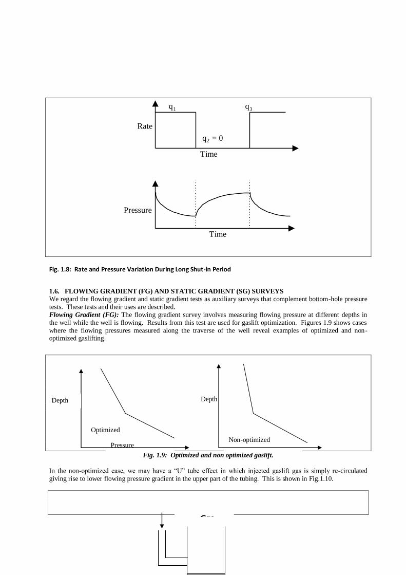
q2 = 0
q3q1
Rate
Time
Time
Pressure
Fig. 1.8: Rate and Pressure Variation During Long Shut-in Period
1.6. FLOWING GRADIENT (FG) AND STATIC GRADIENT (SG) SURVEYS
We regard the flowing gradient and static gradient tests as auxiliary surveys that complement bottom-hole pressure
tests. These tests and their uses are described.
Flowing Gradient (FG): The flowing gradient survey involves measuring flowing pressure at different depths in
the well while the well is flowing. Results from this test are used for gaslift optimization. Figures 1.9 shows cases
where the flowing pressures measured along the traverse of the well reveal examples of optimized and non-optimized gaslifting.
Depth
Fig. 1.9: Optimized and non optimized gaslift.
In the non-optimized case, we may have a “U” tube effect in which injected gaslift gas is simply re-circulated
giving rise to lower flowing pressure gradient in the upper part of the tubing. This is shown in Fig.1.10.
Pressure Pressure
Depth
Optimized
Non-optimized
Gas Gas

Fig. 1.10: Non-Optimized Gaslift
Flowing gradient surveys also provide flowing pressures, which can be used to determine the appropriate
correlation for modelling flow along the wellbore. Such models are used for gaslift optimization. In all cases
during the flowing gradient survey, the depth where pressure was measured is important.
Static Gradient Survey: In this case, we measure pressure at different depths in the well while the well is shut in.
This implies that it can be run in well that has not been flowing. Usually, before a static gradient survey is run, the
well must have been shut in for sufficient time to allow the pressure to stabilize. At every static gradient stop along the well, the gauges must be left for a minimum of 15 minutes so that pressures will be steady.
The static gradient survey is used to determine the fluid distribution in the wellbore. This information is required for
pressure correction and locating the depth for the operating gaslift valves. In a well that is closed in, the static
gradient survey is a good source of pressure data that can be used in calculating the datum pressure with no oil deferred.
The basis for determining fluid gradients using static gradient survey is that fluid gradients depend on the density of
the fluid. Therefore, pressure gradient in the gas zone is small because gas has the smallest density of the wellbore
fluids. Figure 1.11 shows fluid gradients determined using results from static gradient survey in a wellbore that contains gas, oil and water.
Water (0.433 psi/ft)
Pressure, psi
Gas (0.07 psi/ft)
Oil (0.35 psi/ft)Depth, ft
Fig. 1.11: Wellbore Fluid Distribution Determined with Static Gradient Survey

With the static gradient survey, we can determine the gas-oil contact, which is important in selecting the depth of
the gaslift-operating valve. An operating valve that is above the gas-oil contact as shown in Fig. 1.10 will result to
a non-optimized gaslift operation.
To ensure that correct wellbore fluid contacts are determined using static gradient survey, a minimum of two static
survey stops must be taken in each phase as the gauge moves through the fluid phases. Generally, it is recommended that in gaslifted wells, there should be two stops around the region where the gaslift mandrels are
installed. This helps determine fluid contacts (if any) around the gaslift mandrels.
In bottom-hole pressure (BHP) tests, it is required that we measure pressure at the sandface (mid-perforation).
However, in some situations it is not possible for the gauge to be lowered to the sandface. In such situations, the static gradient survey provides the fluid gradient required for obtaining the pressure at the mid perforation. The
equation for calculating the pressure at mid perforation is as follows:
Pmid perf. = Pgauge + (Fluid Gradient x z) 1.1
Where
Pmid perf = Pressure at the mid perforation
Pgauge = Pressure recorded by gauge at the last stop
z = Vertical distance between mid perforation and last gauge stop
Fluid Gradient = Wellbore fluid gradient in the interval z
A graphical interpretation of Eq. 1.1 is shown in Fig. 1.12 for a case where the last gauge depth is the “XN” nipple.
From this, it is obvious that we need to be careful in reporting the gauge depth. An error of 5 ft with water near the
perforations (gradient of 0.433 psi/ft) means a 2.1 psi error and this is more than the absolute accuracy of the crystal
gauges.
Depth
Pressure
Fig.1.12: Extrapolating Pressure to top of Perforation
1.7. COMPLETE BOTTOM-HOLE PRESSURE TESTS PROFILES
A complete buildup or drawdown survey requires that both flowing and static gradient surveys should also be taken.
Typical pressure profiles for such tests are as follows:
XN
Water
Oil
Extrapolation
to mid perf

Flowing Gradient/Buildup/Static Gradient (FG/BU/SG): Typical pressure profile for this test is shown in Fig.
1.13. The sequence of events performed during the test that resulted to the pressure profile shown in Fig 1.13 are as
follows:
Time
Fig 1.13: Pressure Profile for FG/BU/SG Survey
Event Description A – B Gauge in lubricator, reading atmospheric pressure as there is no communication yet with the well
B – C Increasing pressure due to running in hole
C – D Flowing gradient stops
D – E Running in hole to final survey depth E – F Flowtest with gauge at final survey depth
F – G Buildup period
G – H Static Stops near the final survey depth
H – I Pulling gauge out of hole
I – J Static stops in the upper part of tubing for liquid level detection
J – K Pulling gauge out of hole to lubricator
Although events in Fig 1.13 are typical, there may be variations. For example, at the end of
buildup, the gauge may be pulled out about 200 ft and then moved down about 200 ft to original
survey depth. The profile for this case is shown in Fig. 1.14 with events GH and HI representing
the pull out and run back respectively. This could be used for checking the accuracy of depth
measurement as pressure at the same depth in a well that has been shut in for sufficiently long
time must always be the same.
Another variation is a situation where well is shut in while the gauge is run in hole. With the gauge on the bottom,
the well is then opened for a flowtest and then shut-in again for a buildup. A typical profile for this case is shown
in Fig. 1.15.
Increasing
pressure
C
D
E F
G
I
H
Increasing
pressure
A B
C
D
E F
G
H
I
J
K
Flowing Gradient Buildup Static Gradient

Fig 1.14: Pressure Profile for Another FG/BU/SG Survey
Fig 1.15: Pressure Profile for Buildup Survey
If this test is properly run, there will be the advantage of obtaining both buildup and drawdown data that can be
analyzed. Also as the well is shut in while the gauge is run in hole, the problem of lowering gauge especially in high flowrate wells will be eliminated.
The problem with this type of test is that the duration of the shut-in while the gauge is run in
hole may not be adequate for the drawdown and buildup tests to be easily analyzed without
using superposition. That is, the duration may be too short for the system to attain average
pressure, a condition required prior to good drawdown test.
Static Gradient/Drawdown/Flowing Gradient (SG/DD/FG): This is the complete test sequence in a situation where
the well is just programmed for a drawdown. Typical pressure profile for the tests is shown in Fig. 1.16.
Drawdown
Buildup
Gradient stops
Time
Increasing
pressure
Running in hole
Pulling out of hole
Increasing
pressure

Fig 1.16: Pressure Profile for SG/DD/FG Survey
1.8 DEFINITION OF SOME INFORMATION DERIVED FROM BHP TESTS
Most petroleum engineers already know how parameters derived from BHP tests are used. To
our readers who are non-petroleum engineers, this section will help them understand the
importance of some parameters derived from BHP tests.
A. Permeability k: This is a measure of the ability of a formation to allow fluid flow through it. Permeability is
one of the parameters required for rate prediction as shown in the following equations used for rate prediction:
Linear: q (STB/D) = 1.127 x 10 3 KA p
B L
1.2
Radial: q (STB/D) = 7.08 x 10 Kh p
Inr
r
-3
e
w
B
1.3
B. Skin Factor: A measure of the efficiency of drilling and completion practices used. The skin factor can be
used in calculating additional pressure drop around the wellbore caused by drilling and completion practices. Skin
factor is discussed in detail in Chapter 5.
The following are examples of factors that may cause the pressure drop:
1. Alteration of permeability around the wellbore caused by invasion of drilling fluid,
dispersion of clay, mud cake and cement, acidizing etc. In the case of lower permeability
around the wellbore, the skin in this case can be likened to the extra fuel spent in driving
through a bad road.
2. Partial well completion as shown in Fig. 1.17.

Fully completed Partial compleion
Fig. 1.17: Flow Streamlines in Fully and Partially Completed Wells
In the case of a partially completed well, the skin could be likened to the extra energy lost at the door when many
people want to go out (assuming there is fire outbreak in the room) of a room at the same time.
The pressure drop due to skin is wasted because it does not contribute to the useful drawdown.
The skin simply causes an additional pressure drop at the well as shown in Fig. 1.18.
Pressure drop due to skin, pskin, and efficiency are related as follows:
Flow Efficiency (FE) =
P
P
- P - p
- P
wf skin
wf
1.4
Note that the skin and permeability are determined by the amount of pressure change and the rate at which pressure
changes with time. This is shown in Fig. 1.19 for buildup case. This implies that if well is not flowing, there will be no pressure rise and skin and permeability cannot be obtained from the test.

Pwf if no skin
Pwf if there is skin
ps
rw re
useful
drawdown
Fig. 1.18: Pressure Drop Due to Skin
Time
PressureSkin
permeability
P*
Fig. 1.19: Pressure Rise During Buildup
C. Reservoir Drainage Volume: This is the volume of the reservoir drained by test well. Drainage volume is
required in choosing adequate well spacing and reservoir management. Note that wells drain reservoir volumes in
proportion to their rate. This is shown in Fig. 1.20.
D. Porosity : A measure of void spaces in the reservoir. Porosity can be obtained from interference test. Volumetric calculation of initial oil-in-place requires porosity as an input parameter. This is shown in the
equation:

2q.
q.
q.
Fig. 1.20: Relationship between Drainage Area and Rate.
N = 7758 V S
oi`
Boi
. 1.5
E. Average Pressure: This is a measure of reservoir depletion. The amount of fluid in reservoir is related to average pressure in the reservoir. Average pressure is used in material balance calculations.
EXERCISES
1. Explain what is a productivity test
2. Name two important parameters that can be obtained from a bottom-hole pressure test
3. State the uses of BHP derived information
4. Compare and contrast the following:
(a) Drawdown and Buildup tests
(b) Drawdown and interference tests
(c) Buildup and falloff tests
(d) Flowing gradient and static gradient tests
6. Is there any problem with reducing the flowrate to be able to lower your gauges during a BHP
survey? Explain
7. Give typical values of gas, oil and water gradients.
8. Static pressures at two points that are 213 ft apart along the well are 3550 psi and 3463.4 psi. The angle of
deviation in region of interest is 20o. Calculate the fluid gradient in the region of the wellbore assuming (a)
no deviation correction. (b) deviation correction. What fluid is in that section of the wellbore?
9. The following information was obtained during a survey
Gauge depth = 6000ftss
Fluid gradient at gauge depth = 0.433 psi/ft Gauge depth to mid perforation = 300ft (vertical depth)
Datum depth = 6200ftss
Reservoir Oil Gradient = 0.35 psi/ft
Pressure at Gauge depth = 2500 psia

Using the supplied information calculate the following
(a) Pressure at mid perforation
(b) Datum pressure
10. Draw the rate and pressure profiles of the following tests: (a) Drawdown test
(b) Flowing Gradient / Buildup / Static Gradient
(c) Interference tests in a situation where fluid was injected into the active well before it was shut-in.
Show the pressure profile in both active and observation well.
11. Figure 1.21 shows pressure pertubation obtained during a BHP test. State the causes and implications on
test.
Fig. 1.21
4. INTRODUCTION
Oil well tests are made for numerous reasons and the type of test required depends on the objective of the test.
Common well tests include:
(a) Potential test
(b) Gas-oil ratio test
(c) Productivity test
(d) Bottom-hole pressure test

Potential test involves measurement of the amount of oil and gas a well produces during a given period (normally
24 hours or less) under certain conditions fixed by regulatory bodies. The information obtained from these tests is
used in assigning a producing allowable of the well. The gas-oil ratio test is made to determine the volume of gas
produced per barrel of oil so as to ascertain whether or not a well is producing gas in excess of permissible limit.
Bottom-hole pressure test involves measurement of sandface pressure and flowrate variation with time. Such tests are quite economical to run and they yield valuable information about the reservoir characteristics and well
characteristics. Hence, bottom-hole pressure tests are usually referred (Earlougher, 1977; 1982) to as welltests.
Productivity tests are made on oil wells and include both the potential test and the bottom-hole pressure (BHP) test.
The purpose of this test is to determine the effects of different flow rates on the pressure within the producing zone
of the well and thereby establish producing characteristics of the producing formation. In this manner, the
maximum potential rate of flow can be calculated without risking possible damage to the well which might occur if
the well were produced at its maximum possible flow rate.
In this book, the term welltest will be used for bottom-hole pressure test unless otherwise stated. In this chapter, the
purpose of well testing, types of well tests and well test equipment are discussed. In addition, other practical
aspects of BHP tests such as test procedure and equipment problems are discussed.
1.1 OBJECTIVES OF BHP SURVEY
Bottom-hole pressure tests are conducted to obtain data that can be used for the following
purposes:
Determine Well Parameters
- Skin
- Productivity Index
- Wellbore storage constant
- Fluid distribution in wellbore
- Flowing pressures in wellbore
- Static gradients
Determine Reservoir Parameters
- Average pressure in the drainage area
- Permeability - Distance to boundaries
- Vertical/Horizontal permeability
- Gas/oil contacts
Determine Dynamic Influence of other Wells/Aquifer
Assess Changes Since Previous Survey
- Changes in datum pressure
- Changes to damage skin - Changes in drainage area (from a drawdown test)
- Confirm boundaries
1.2 USES OF BHP DERIVED INFORMATION
Results obtained from BHP tests are used for the following purposes:
* Reservoir Surveillance

* Determination of Stimulation Candidates
* Gaslift Optimisation
* Input for Reservoir Simulation
* Material Balance Calculation
Examples of benefits from BHP test compiled by a client are given in Table 1.1. The benefits were realised by using results from BHP tests for good well and reservoir surveillance.
Table 1.1: Benefits from BHP Surveys
ACTIVITIES SAVINGS
($ million)
Well Surveillance
Stimulation (abort 5 jobs, contribute to finding 5 more)
Gaslift Optimization (10% improvement of target at $1/bbl)
0.8
1.0
Reservoir Surveillance
Sand F4.0/F4.1X Production (3 Mbopd) 1.0
Sand-X Block (new well cancelled) 3.0
Dump Creek (10% of the 6 fewer wells required) 3.0
Well -11 (sidetrack raise trajectory) 1.0
Sand D5.0X Development
(horizontal well changed to recompletion) 3.0
(10% of 8 well campaign) 4.0
Total 16.8
1.3 COMMON TYPES OF BOTTOM-HOLE PRESSURE (BHP) TESTS
Common types of bottom-hole pressure tests include the following:
(g) Drawdown test
(h) Injectivity test
(i) Buildup test
(j) Falloff test
(k) Interference/pulse tests (l) Others
The definitions of the tests and the rate and pressure profiles during the test are as follows:
1. Drawdown Test: Involves measuring the variation of sandface pressure with time while the well is flowing.
For a drawdown test, the well must have been shut in to attain average pressure before production commences for
the test. The rate and pressure profiles during drawdown test are in Fig 1.1.

Pwf
0 timetime
q
0
Fig. 1.1: Rate and Pressure Profiles During Drawdown Test
5. Injectivity Test: This is the counterpart of a drawdown test and involves measuring the variation of sandface
pressure with time while fluid is being injected into the well. The rate and pressure profiles during drawdown
test are in Fig 1.2.
q Pwf
0 time
Injection (-ve q)
time
Fig. 1.2: Rate and Pressure Profiles During Injectivity Test
3. Buildup Test: Involves measuring the variation of sandface pressure with time while well is shut-in. The
well must have flowed before shut-in. Figure 1.3 shows the rate and pressure profiles during the flow and buildup
periods. Buildup tests are more common and will be the main subject of our discussion.
Pw
0 time 0 time
q
Shut-in Time
0
Drawdown
Buildup
Drawdown
Buildup
Fig. 1.3: Rate and Pressure Profiles During Drawdown and Buildup

11. Falloff Test: This is the counterpart of buildup test and it involves measuring the variation of sandface pressure
with time while well is shut-in. In this case, some fluid must have been injected into the well before shutting.
Figure 1.4 shows the rate and pressure profiles during the injection and falloff periods.
q Pw
0 time
Injection
time
Fig. 1.4: Rate and Pressure Profiles During Injectivity and Falloff Test
12. Interference Test: Unlike the first four tests (drawdown, injectivity, buildup, falloff) which are tests involving
only one well (single well tests), the interference test involves the use of more than one well (multiple well
test). During interference tests, pressure changes due to production or injection or shut-in at an active well is
monitored at an observation well. The active well and the observation well are shown in Fig 1.5. Only one
active well is required, but there could be more than one observation well.
Interference tests are primarily used to establish sand continuity between the active and observation wells. In
situation where more than one observation well is used, interference test can be used to find (Ramey and )
maximum and minimum permeability and their directions.
Active Well Observation Well
Sand continuityGauge
q > 0
q = 0
q < 0
q = 0
Fig. 1.5: Active and Observation Wells in an Interference Test
1.4 IDEAL CONDITIONS AND INFORMATION DERIVED FROM TEST
If possible, BHP tests should be run under the stated ideal conditions as this makes interpreting such tests easy. The
ideal conditions for running different BHP tests and information that can be obtained from the tests are given in
Table 1.2
Table 1.2: Types of Well Tests and Derivable Information
Type of Test Ideal Conditions for Test Information Derived from Test
Injectivity Falloff
Shut-in

Drawdown 1. Constant rate production
2. Well shut-in long enough before test
to attain uniform pressure in
reservoir.
1. Permeability
2. Skin factor
3. Reservoir drainage volume
4. Flow efficiency
5. Distance to linear no-flow barrier
Buildup 1. Constant rate production before
shut-in.
1. Permeability
2. Skin factor
3. Flow efficiency
4. Average Pressure
5. Distance to linear no-flow barrier
Interference 1. Constant rate production or injection
at the active well.
1. Permeability
2. Storativity 3. Anisotropic permeability
values and orientation
4. Sand continuity
1.5 IMPORTANCE OF STICKING TO IDEAL CONDITION FOR TEST
In this section, we shall discuss the importance of sticking to the ideal condition for any test. Two factors
considered are constant rate production and not shutting well for long period before a drawdown test.
(1) Constant Rate Production: Rate variation makes tests difficult to analyse because effect of rate changes last
until well is shut-in and builds up to average pressure. Rate changes are modelled using the concept superposition
illustrated in Fig. 1.6. Figure 1.6 shows that a rate which occurred at where at time, t, will continue to affect
pressure response until time, t + t. In a layman’s language, wells do not forget rate changes that occurred in them
unless they are shut in to build up to average pressure.
q1
q2
q1
- q1
q2+
t
t + tt t
Fig. 1.6: Effect Rate Variation
Causes of Rate Variation
Some tests like the potential tests are designed such that the rates in the wells are varied. Such rate variations create
no problem during analysis because the rates are measured and therefore can be considered during analysis.
Situations that create problems include cases where the rates are varied and not measured. Such situations may
occur under the following conditions:
(a) Partly closing wing value to lower tools
(d) Slow shutting of well at end of flowtest
(e) Not allowing for rate stabilization. Surface indications of well stabilization include
(i) Constant wellhead flowing pressure

(ii) Constant gas production rate
(iii) Constant fluid production rate.
(2) Long shut-in Requirement: The rate and pressure profiles for wells shut-in for long and short times are
shown in Fig. 1.7 and Fig. 1.8.
Short Shut-in Period
q2 = 0
q3
q1
Rate
Time
Time
Pressure
Fig. 1.7: Rate and Pressure Variation During Short Shut-in Period
Long Shut-in Period
q2 = 0
q3q1
Rate
Time
Time
Pressure
Fig. 1.8: Rate and Pressure Variation During Long Shut-in Period
For the case of short shut-in period, the well did not build up to the average pressure before the drawdown test was
started. In this case, analysis of the test will involve using three rates.

However, for the case of long shut-in time before the drawdown, the well reached the average pressure during the
buildup. Hence, analysis of the drawdown will simply involve a single rate. A single rate test is usually simpler to
analyse than a three rate test.
1.6. FLOWING GRADIENT (FG) AND STATIC GRADIENT (SG) SURVEYS
We regard the flowing gradient and static gradient surveys as auxiliary surveys that complement bottom-hole pressure tests. These tests and their uses are described.
Flowing Gradient (FG): The flowing gradient survey involves measuring flowing pressure at different depths in
the well while the well is flowing. Results from this test are used for gaslift optimization. Figures 1.9 shows cases
where the flowing pressures measured along the traverse of the well reveal examples of optimized and non-
optimized gaslifting.
Depth
Fig. 1.9: Optimized and non optimized gaslift.
In the non-optimized case, we may have a “U” tube effect in which injected gaslift gas is simply re-circulated
giving rise to lower flowing pressure gradient in the upper part of the tubing. This is shown in Fig.1.10.
Gas Gas
Fig. 1.10: Non-Optimized Gaslift.
Flowing gradient surveys also provide flowing pressures which can be used to determine the appropriate correlation
for modelling flow along the wellbore. Such models are used for gaslift optimization. In all cases during the
flowing gradient survey, the depth where pressure was measured is important.
Static Gradient Survey: In this case, we measure pressure at different depths in the well while the well is shut in. This implies that it can be run in well that has not been flowing. Usually, before a static gradient survey is run, the
well must have been shut in for sufficient time to allow the pressure to stabilize. At every static gradient stop along
well, the gauges must be left for a minimum of 15 minutes so that pressures will be steady.
The static gradient survey is used to determine the fluid distribution in the wellbore. This information is required
for pressure correction and locating the depth for the operating gaslift valves. In a well that is closed in, the static
gradient survey is a good source of pressure data that can be used in calculating the datum pressure with no oil
deferred.
Pressure Pressure
Depth
Optimized
Non-optimized

The basis for determining fluid gradients using static gradient survey is that fluid gradients depend on the density of
the fluid. Therefore, pressure gradient in the gas zone is small because gas has the smallest density of the wellbore
fluids. Figure 1.11 shows fluid gradients determined using results from static gradient survey in a wellbore that
contains gas, oil and water.
Water (0.433 psi/ft)
Pressure, psi
Gas (0.07 psi/ft)
Oil (0.35 psi/ft)Depth, ft
Fig. 1.11: Wellbore Fluid Distribution Determined with Static Gradient Survey
With the static gradient survey, we can determine the gas-oil contact which is important in selecting the depth of the
gaslift operating valve. An operating valve that is above the gas-oil contact as shown in Fig. 1.10, will result to a
non-optimized gaslift operation.
To ensure that correct wellbore fluid contacts are determined using static gradient survey, a minimum of two static
survey stops must be taken in each phase as the gauge moves through the fluid phases. Generally, it is
recommended that in gaslifted wells, there should be two stops around the region where the gaslift mandrels are
installed. This helps determine fluid contacts (if any) around the gaslift mandrels.
In bottom-hole pressure (BHP) tests, it is required that we measure pressure at the sandface (mid-perforation).
However, in some situations it is not possible for the gauge to be lowered to the sandface. In such situations, the
static gradient survey provides the fluid gradient required for obtaining the pressure at the mid perforation. The
equation for calculating the pressure at mid perforation is as follows:
Pmid perf. = Pgauge + (Fluid Gradient x z) 1.1
Where
Pmid perf = Pressure at the mid perforation
Pgauge = Pressure recorded by gauge at the last stop
z = Distance between mid perforation and last gauge stop
Fluid Gradient = Wellbore fluid gradient in the interval z
A graphical interpretation of Eq. 1.1 is shown in Fig. 1.12 for a case where the last gauge depth is the “XN” nipple.
From this, it is obvious that we need to be careful in reporting the gauge depth. An error of 5 ft with water near the
perforations (gradient of 0.433 psi/ft) means a 2.1 psi error and this is more than the absolute accuracy of the crystal
gauges.
XN
Water
Oil

Depth
Pressure
Fig.1.12: Extrapolating Pressure to top of Perforation
1.7. COMPLETE BOTTOM-HOLE PRESSURE TESTS PROFILES
A complete buildup or drawdown survey requires that both flowing and static gradient surveys should also be taken.
Typical pressure profiles for such tests are as follows:
Flowing Gradient/Buildup/Static Gradient (FG/BU/SG): Typical pressure profile for this test is shown in Fig.
1.13.
Time
Fig 1.13: Pressure Profile for FG/BU/SG Survey
The sequence of events performed during the test that resulted to the pressure profile shown in Fig 1.13 are as
follows:
Event Description A – B Gauge in lubricator reading atmospheric pressure as there is no communication yet with the well
B – C Increasing pressure due to running in hole
C – D Flowing gradient stops
D – E Running hole to final survey depth
E – F Flowtest with gauge at final survey depth
F – G Buildup period
G – H Static Stops near the final survey depth H – I Pulling gauge out of hole
I – J Static stops in the upper part of tubing for liquid level detection
J – K Pulling gauge out of hole to lubricator
Extrapolation
to mid perf
Increasing
pressure
A B
C
D
E F
G
H
I
J
K
Flowing Gradient Buildup Static Gradient

Although events in Fig 1.13 are typical, but there may be variations. For example, at the end of buildup, the gauge
may be pulled out about 200 ft and then moved down about 200 ft to original survey depth. The profile for this case
is shown in Fig. 1.14 with events GH and HI representing the pull out and run back respectively. This could be
used for checking the accuracy of depth measurement as pressure at the same depth in a well that has been shut in
for sufficiently long time must always be the same.
Another variation is that of where well is shut in while the gauge is run in hole. With the gauge on the bottom, the
well is then opened for a flowtest and then shut-in again for a buildup. A typical profile for this case is shown in
Fig.1.15.
Fig 1.14: Pressure Profile for Another FG/BU/SG Survey
Fig 1.15: Pressure Profile for Buildup Survey
Drawdown
Buildup
Gradient stops
Time
Increasing
pressure
Running in hole
Pulling out of hole
Increasing
pressure
A B
C
D
E F
G
I
J
Flowing Gradient Buildup Static Gradient
Time
H

If this test is properly run, there will be the advantage of obtaining both buildup and drawdown data that can be
analyzed. Also as the well is shut in while the gauge is run in hole, the problem of lowering gauge especially in
high flowrate wells will be eliminated.
The problem with this type of test is that the duration of the shut-in while the gauge is run in hole may not be adequate for the drawdown and buildup tests to be easily analyzed without using superposition. That is, the
duration may be too short for the system to attain average pressure, a condition required prior to good drawdown
test.
Static Gradient/Drawdown/Flowing Gradient (SG/DD/FG): This is the complete test sequence in a situation where
the well is just programmed for a drawdown. Typical pressure profile for the tests is shown in Fig. 1.16.
Fig 1.16: Pressure Profile for SG/DD/FG Survey
1.9 USES OF INFORMATION DERIVED FROM BHP TESTS
Most petroleum engineers already know how parameters derived from BHP tests are used. To
our readers who are non-petroleum engineers, this section will help them understand the
importance of some parameters derived from BHP tests.
A. Permeability k: This is a measures of the ability of a formation allow fluid flow through it. Permeability is one
of the parameters required for rate prediction as shown in the following equations used for rate prediction:
Linear: q (STB/D) = 1.127 x 10 3 KA p
B L
Radial: q (STB/D) = 7.08 x 10 Kh p
Inr
r
-3
e
w
B
Static Gradient Drawdown Flowing Gradient
Time
Increasing
pressure

B. Skin Factor: A measure of the efficiency of drilling and completion practices used. The skin factor can be
used in calculating additional pressure drop around the wellbore caused by drilling and completion practices.
Skin factor is discussed in detail in Chapter ????
The pressure drop may be caused by the following:
1. Alteration of permeability around the wellbore caused by invarion of drilling fluid, dispersion of clay, mud
cake and cement, acidizing etc. In the case of lower permeability around the wellbore, the skin in this case can
be likened to the extra fuel spent in driving through a bad road.
2. Partial well completion as shown in Fig 1.17.
Fully completed Partial compleion
Fig. 1.17: Flow Streamlines in Fully and Partially Completed Wells
In the case of a partially completed well, the skin could be likened to the extra energy lost at the door when many
people want to go out (assuming there is fire outbreak in the room) of a room at the same time.
The pressure drop due to skin is wasted because it does not contribute to the useful drawdown. The skin simply
causes an additional pressure drop at the well as shown in Fig. 1.18.
Pwf if no skin
Pwf if there is skin
ps
rw re
useful
drawdown
Fig. 1.18: Pressure Drop Due to Skin
Pressure drop due to skin, pskin , and efficiency are related as follows:
Flow Efficiency (FE) = P
P
- P - p
- P
wf skin
wf
Note that the skin and permeability are determined by the amount of pressure rise and the rate at which pressure
rises with time. This is shown in Fig. 1.19. This implies that if pressure does not rise, there will be no pressure rise and skin and permeability cannot be obtained from the test.

Time
PressureSkin
permeability
P*
Fig. 1.19: Pressure Rise During Buildup
C. Reservoir Drainage Volume: This is the volume of the reservoir drained by test well. Drainage volume is
required in choosing adequate well spacing and reservoir management. Note that wells drain reservoir volumes in
proportion to their rate. This is shown in Fig 1.20.
2q.
q.
q.
Fig. 1.20: Relationship between Drainage Area and Rate.
D. Porosity : A measure of void spaces in the reservoir. Porosity can be obtained from interference test. Volumetric calculation of initial oil-in-place requires porosity as an input parameter. This is shown in the equation:
N = 7758 A Soi
Boi.
E. Average Pressure: This is a measure of depletion as the amount of fluid in reservoir is related to average
pressure in the reservoir. Average pressure is used in material balance calculations.
END of Chapter 1
1.7 WELL TEST EQUIPMENT
(1) Pressure recorders
(2) Lubricator (Wireline BOP) (3) Wireline unit
(4) Christmas tree with hydraulically operated value
A schematic of the arrangement taken from Dake (??/) is shown in Fig 1.20 while Fig, 1,21 shows more detail.

Fig. 1.20: Welltest Equipment
Leave a page for the next diagram???
Figure 1.21: Wireline Surface Equipmwnt
(Example of an Arrangement)
Pressure Gauges
Different types of gauges are used for measuring bottom-hole pressure. The sensitivity and the accuracy of the
gauges vary. The accuracy of a gauge is principally concerned with systematic errors, often attributed to the
calibration of the gauge. For example, if the accuracy of a gauge is 5 psi and gauge reads 1000 psi, this implies that
the correct readings lie in the range (1000-5) psi to (1000+5)psi.
The sensitivity or resolution of a gauge is described as the smallest pressure that can be reliably measured by the
gauges. Table 1.3 shows bottom-hole pressure measured in a Niger Delta well with an insensitive gauge. The
constant pressure which became constant after a shut-in time of 3 minutes is not necessarily due to stabilization, but
the gauge could not “discern” the pressure changes with time.
Table 1.3: Buildup Data from Niger Delta Well
Shut-in Time, min Shut-in Pressure, psi
1 3488
2 3531
3 3539
5 3539
10 3539
20 3539
30 3539
40 3539
50 3539
60 3539
90 3539
120 3539
The types of gauges, principle of operation, accuracy and sensitivity are give in Table 1.4.
Tables 1.4: Types of Gauges and Operation Principles
Type of Gauge Principle of Operation Accuracy Sensitivity
Amerada
Strain Gauge
Quartz Crystal (Electronic)
Bourdon tube (Mechanical)
Change in resistivity
Change in frequency
0.2% FSD
0.05% FSD
0.035% R
0.05% FSD
0.0025% FSD
0.0001% FSD
FSD = Full Scale Deflection, e.g. 5000 or 10.000 psi
R = Reading, i.e. the measured pressure
The implications of information in Table 1.4 for a 5000 psi and 10,000 psi rated gauges are shown in Table 1.5.
Table 1.5: Sensitivity and Accuracy of 5000 psi and 10000 psi Rated Gauges
Type of Gauge FSD = 5000 psi FSD = 10,000 psi
Accuracy Sensitivity Accuracy Sensitivity
Amerada 10 psi 2.5 psi 20 psi 5.0 psi

Strain Gauge 2.5 psi 0.125 psi 5.0 psi 0.25 psi
Quartz Crystal
(Electronic)
1.75 psi 0.005 psi 3.5 psi 0.01 psi
For the electronic gauge, the calculated sensitivity is the maximum because we assumed that the measured pressure
is equal to the Full Scale Deflection (FSD). Some deduction from Table 1.4 and 1.5 are as follows:
1. The electronic gauges are more sensitive and accurate than the strain gauge while the strain gauge is more
sensitive and accurate than the Amerada gauge.
2. If a 5000 psi gauge can do the job, do not use a 10000 psi gauge because the 10000 psi gauge has lower
accuracy and sensitivity.
Ideally, we recommend that electronic gauges be used. However, it costs more than other gauges, but it is worth it.
Amerada Gauges Until 1994 about 80% of bottom-hole pressure tests in Nigeria are ran with Amerada gauges. Now most companies
in Nigeria do not use them. However, for historical reasons, we need to discuss the Amerada gauge because it
clearly shows the components of any gauge: a clock, pressure sensor and recorder. Figure 1.22 is a schematic of the
Amerada gauge. The continuous trace of pressure versus time is made by the contact of a stylus with a chart, which
has been specially treated, on one side to permit the stylus movement to be permanently recorded. The chart is held
in a cylindrical chart holder that is in turn connected to a clock which drives the holder in the vertical direction. The
stylus is connected to a bourdon tube and is constrained to record pressures in the perpendicular direction to the
movement of the chart holder. The combined movement is such that, on removing the chart from the holder after
the survey, a continuous trace of pressure versus time is obtained as shown in Fig. 1.22b, for a typical pressure buildup survey.
Fig 1.22 Here ????
1.8 ELECTRONIC GAUGES AND PROBLEMS For BHP surveys, the electronic gauges have now replaced the Amerada gauges. The electronic gauges are more
sensitive and accurate, but they are also more delicate and require regular calibrations. Figures 1.10 to 1.19 show
pressures measured with electronic gauges and problems associated with the measurements. The problems include
gauge “shifts,” vibrations, synchronization, failure, etc.
Buildup Survey: The buildup survey involve measuring pressure variation with time with the gauges at a fixed
location. The buildup survey is always preceeded by a flowing test which involves flowing the well for about six
hours with the gauges at the last flowing gradient survey depth. This is necessary to allow for flow stabilization and
to get big enough reservoir response before shutting in. A typical pressure profile during the flow-test and buildup
periods is shown in Fig. 1.25.
Some information derived from the test include P*, Skin and permeability.
1.10 FLOWING GRADIENT/BUIDUP/STATIC GRADIENT SURVEY PROPOSAL
A typical FG/BU/SG survey proposal is in Appendix A. Some of the information in the proposal and reasons
for including such information are discussed. We shall discuss Page A.1 to Page A.8.
Page A.1: Contains the following information:

(a) Objectives of test,
(b) Types of tests required
(c) Depth reference data (DFE, CHH).
The objectives of a tests and types of tests required are related. For example, if one of the objectives is to
optimize gaslift, a flowing gradient survey must be included as one of the test. Also, for us to calculate P*, skin and permeability, both buildup and static gradient surveys must be included. Always match the survey required with the
objectives of the survey.
The depth reference (DFE and DFE - CHH) shows the basis for calculating depths with reference to the
casing head. The BHP contractor should ensure that stated depth reference agrees with what is in the status
diagram.
Page A.2: Main information on this page of the proposal are as follows:
(a) Production rate
(b) Perforated Interval
(c) Location of sleeve and nipple
Good rate data is as important as the pressure measurements. We therefore recognize the important role that flowstation staff play in giving us accurate rate data. The BHP contractor should always check with the flowstation
staff and confirm that the stated rate is the current rate. There is no point running a flowing gradient and buildup
surveys in well that is not flowing. Even in flowing wells, the contractor should check the rate and ascertain that
the gauges can be run in hole while the well is flowing. The proposal states on Page A.4 that if the gauges cannot
be run hole at the current rate, the rate should be adjusted (i.e. change bean size) 24 hours before test. Changing
bean size requires contacting production staff. We expect that the BHP contractor will be guided by his experience.
Perforated interval is an important data because we are interested in the pressure at the middle of the
perforation. In tests run in the long string, the gauges can be lowered, in most cases, to the top of the perforation.
This is not possible for tests run in the short strings because of the “Amerada” stops which will not allow gauges
pass through them.
In all cases where the gauges can be lowered to the top of the perforation, the BHP contractor is advised to do so because that minimize phase segregation effects and minimizes errors in correcting to the top of the
perforation. In situations where the gauges cannot be lowered to the perforations, static gradient stops should be
taken at short intervals so that type of fluid at bottom can be determined. We need this information for correcting
pressure to the top of the perforation.
The BHP contractor should note the positions of the nipple and sleeve as they are needed for depth control.
Depths in the proposal must be cross checked with the status diagram. Also, the speed at which the wireline is
lowered should be reduced in areas where there are restrictions in the well to avoid hitting the gauges against these.
Gauges are sensitive and can easily be damages.
Page A.3: This page gives gauge specification, information on the following:
(a) Gauge specification
(b) Sampling rate (c) Depth Control procedure
The BHP contractor should ensure that their gauges meet stated specifications. Usually, we recommend that
two gauges be used in surveys. This must be adhered to because readings from both gauges are used for gauge
quality check. Also, in a situation where one gauge fails, we can still rely on readings from only one gauge.
Using the sampling rate in the proposal in important. Many changes in sampling rate during a survey is not
welcome because we have observed pressure shift, as much as 3 psi, caused by change in sampling rate. Such
pressure shifts cause discontinuities that may make analysis of test difficult and results obtained from such tests
may be unrealistic.
We wish to encourage BHP contractors to consider depth control as a very important issue. because the depth at which pressure was measured is as important as the pressure measurements. The contractors are advised to follow

the recommended procedure and document locations of sleeve and nipple if they are different from what is in the
status diagram. If the BHP analyst knows the measured depths he can correct the recorded pressure to the reference
depth. But if the analyst does not know the depth, he cannot make such correction.
Page A-4: This page contains information on the following:
(a) Well conditioning (b) Gauge Quality Control
Well conditioning is required to ensure that well produced at stable conditions before shut-in. Normally, no
time should be spent on well conditioning if rate was not changed while the gauges were run in hole or during the
flowtest. This is the reason why all required rate changes should occur at least 24 hours before test commences.
Quality checks on gauge measurements are required so that the BHP contractor will detect anomalies in the
performance of their gauges. SPDC also performs their own quality checks.
Page A-5: This page shows the flowing gradient stops and the duration of the stops. There must be at least two
stops around the gaslift mandrels if the flowing pressures will be used in vertical lift performance studies and
determining correct gaslift locations.
Page A-6: This page contains information on the following
(1) The duration of the flowtest
(2) The duration of the build up test
(3) Data to be gathered during the flowtest
The duration of the flowtest does not include whatever time it takes to run in hole and perform the flowing
gradient survey. The gauges must be at the final survey during the flowtest. If the gauges are moved, the flowtest
should be repeated. Measurements to be taken during the flowtest include the THP, THT, GOR and flowrate.
These parameters should be measured every 15 minutes during the flowtest.
In Page A-6, there is also instruction on the need to secure the well with the gauges at fixed location in cases
where the well will be shut-in overnight. This is to ensure that there is no slippage or tampering.
Page A-7: This gives information on the location of the static gradient stops and the duration of the stops. It is
important to note the following:
(a) The distance between stops should be smaller around the final survey depths. This is important because we
need to accurately determine the fluid gradient required for pressure correction.
(b) There must be at least two stop around the gaslift mandrels so that the gas/oil contact (if any) can be
determined accurately.
(c) Measurement of the static oil gradient is useful for estimating the oil density in the reservoir.
1.11 USEFUL HINTS ON PROPER TESTING OF WELLS
(a) The gauges must be in good conditions to record accurate pressure.
(b) Depths where the pressure measurement are taken must be known.
(c) Correct stable flowrate must be known during flowing gradient survey and prior to shut-in.
(d) Sufficient gaslift pressure must be available for reliable stable flow of gaslifted intervals.
(e) Survey programme must be understood and followed.
A summary of the procedure for running FG/BU/SG survey is as follows:
1. Perform dummy run to determine hold-up-depth (HUD). Locate XN-Nipple and mark wireline. Why?
2. Run in hole both gauges to specified depths while well is flowing. Use wireline mark
as depth control. 3. Suspend gauges at final survey depth and allow flow to continue for the specified
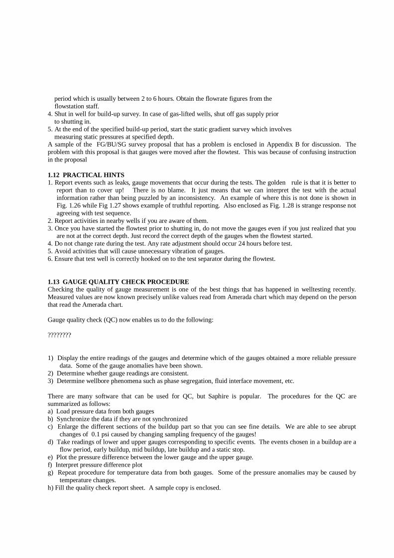
period which is usually between 2 to 6 hours. Obtain the flowrate figures from the
flowstation staff.
4. Shut in well for build-up survey. In case of gas-lifted wells, shut off gas supply prior
to shutting in.
5. At the end of the specified build-up period, start the static gradient survey which involves
measuring static pressures at specified depth. A sample of the FG/BU/SG survey proposal that has a problem is enclosed in Appendix B for discussion. The
problem with this proposal is that gauges were moved after the flowtest. This was because of confusing instruction
in the proposal
1.12 PRACTICAL HINTS 1. Report events such as leaks, gauge movements that occur during the tests. The golden rule is that it is better to
report than to cover up! There is no blame. It just means that we can interpret the test with the actual
information rather than being puzzled by an inconsistency. An example of where this is not done is shown in
Fig. 1.26 while Fig 1.27 shows example of truthful reporting. Also enclosed as Fig. 1.28 is strange response not
agreeing with test sequence.
2. Report activities in nearby wells if you are aware of them.
3. Once you have started the flowtest prior to shutting in, do not move the gauges even if you just realized that you are not at the correct depth. Just record the correct depth of the gauges when the flowtest started.
4. Do not change rate during the test. Any rate adjustment should occur 24 hours before test.
5. Avoid activities that will cause unnecessary vibration of gauges.
6. Ensure that test well is correctly hooked on to the test separator during the flowtest.
1.13 GAUGE QUALITY CHECK PROCEDURE
Checking the quality of gauge measurement is one of the best things that has happened in welltesting recently.
Measured values are now known precisely unlike values read from Amerada chart which may depend on the person
that read the Amerada chart.
Gauge quality check (QC) now enables us to do the following:
????????
1) Display the entire readings of the gauges and determine which of the gauges obtained a more reliable pressure
data. Some of the gauge anomalies have been shown.
2) Determine whether gauge readings are consistent.
3) Determine wellbore phenomena such as phase segregation, fluid interface movement, etc.
There are many software that can be used for QC, but Saphire is popular. The procedures for the QC are
summarized as follows: a) Load pressure data from both gauges
b) Synchronize the data if they are not synchronized
c) Enlarge the different sections of the buildup part so that you can see fine details. We are able to see abrupt
changes of 0.1 psi caused by changing sampling frequency of the gauges!
d) Take readings of lower and upper gauges corresponding to specific events. The events chosen in a buildup are a
flow period, early buildup, mid buildup, late buildup and a static stop.
e) Plot the pressure difference between the lower gauge and the upper gauge.
f) Interpret pressure difference plot
g) Repeat procedure for temperature data from both gauges. Some of the pressure anomalies may be caused by
temperature changes.
h) Fill the quality check report sheet. A sample copy is enclosed.

Inferences that can be made from the pressure difference plot for two gauges that were placed 4 ft apart are as
follows:
i) The pressure difference will reflect the fluid in the 4 ft column between the gauges
ii) If the 4 ft column is filled with gas, the pressure difference will be smaller than if the column was filled with
liquid iii) Ideally the maximum pressure difference will be 4 ft x 0.433 psi/ft (water gradient) = 1.732 psi. Getting
pressure differences as high as 3 psi shows that something is wrong with one of the gauges or both gauges.
Figures 1.29 and 1.30 show pressure and temperature differences from two tests. In Fig.1.29 pressure difference
was constant and this implies that there was no gas segregation. In Fig. 1.30, there is evidence of gas segregation.
The pressure difference was initially low and later increased as gas bubbled out leaving a denser fluid. Detecting
these phenomenon helps while analyzing tests because non-reservoir responses will not be interpreted.
Figure 1.31 shows quality check in which fine details are revealed while Fig. 1.32 is a quality check plot showing
unrealistic pressure differences for gauges that are just 4 ft apart. Figure 1.33 is a quality check plot showing the
effect of leak while Fig. 1.34 shows the effect of liquid interface movement.
1.14 ROLES OF FIELD STAFF IN BHP SURVEY
Field staff involved in BHP survey are production staff and BHP contractor staff. The role played by both
is vital for good data to be obtained. Also, both production and BHP contractor staff need to understand the
principles involved in BHP test and analysis. These principles are illustrated in Fig. 1.35
Reservoir
k? s?
Pressure change
(Output)
Model
k, s, etc known
Same
Rate change
Rate change
(Input)
(Input) (Output)
Pressure change
Test Principle
Analysis Principle
Fig. 1.35: Test and Analysis Principles
The test principle involves allowing some known rate changes to occur in the reservoir and measuring the resulting
pressure changes. Note that some characteristics of the reservoir such as the permeability are not known.
Analysis principle involves applying the same rate changes to a mathematical model whose characteristics are
known and observing the resultant pressure changes. The model characteristics can be changed until the pressure
changes from the model become equivalent to pressure changes obtained when the same input (rate changes) were
applied to the reservoir. We now conclude that the model characteristics are equivalent to the reservoir
characteristics.
The implications of the test and analysis principles are as follows:
1.) Rate changes are needed to create pressure changes.
2.) Correct rate (input) applied to the reservoir must be known.

???????????
3.) Unrecorded rate changes render test less reliable or useless even in some cases.
4.) Correct pressure changes caused by rate changes must be measured.
5.) Factors such as leak, gauge movement, etc. cause pressure changes not associated with rate changes.
1.14.1 Roles of Production Staff
Production staff benefit from results obtained by analyzing BHP tests because such tests are used for good well and
reservoir management. We are sure everyone is happy when wells are producing at optimum rate. The production
staff can contribute very much to the success of any BHP survey by doing the following:
1.) Ensuring that a full flowtset is conducted prior to shutting in the well for buildup. Note that the BS&W
and GOR are also required during test analysis.
2.) Ensuring that the correct well is hooked on for test.
3.) Reporting everything that could introduce errors in recorded production rate (e.g. zero rate tests, changes to
gaslift availability, surging).
4.) Telling the BHP contractor the correct status of well before survey starts. 5.) Taking more interest in BHP surveys. After all, we are all partners in progress.
1.14.2 Roles of BHP Contractor Staff
The success of BHP survey depends heavily on the field staff that runs the test. A few things the field staff should
be aware of are summarized as follows:
1.) A well that is not flowing or a well that cannot be shut in will not produce the required pressure change
needed for good analysis of buildup test.
2.) Moving gauges when they are required to be at a certain position will produce pressure changes that will
distort the correct pressure changes induced by applied rate changes..
3.) Due to the relationship between depth and pressure, good depth control is needed so that we can associate
pressure with correct depths. 4.) Leaks are unwelcome events because they affect pressure changes.
5.) Good gauges are always needed for correct pressure measurements.
6.) Mistakes give rise to wrong interpretations and wasted resources.
7.) Cooperation with flowstation staff is necessary.
8.) Accurate reporting of all deviations from programme. If the test analyst knows, he may be able to
compensate for deviations.
2. BASICS OF ANALYZING BOTTOM HOLE TESTS
In this section, we shall discuss the phases through which a test well goes through. We shall
consider only the drawdown and buildup tests. We shall discuss methods of identifying the
phases.
2.1 FLOW PHASES
Draw down test

Wellbore Storage phase
AB
Transient phase Boundary Effect phase
Increasing Time
Figure 2.1: Flow Phases in Drawdown Test.
Wellbore Storage
AB
Transient phase
phase
Stabilization
Increasing Shut-in Time
Figure 2.2: Flow Phases in Buildup Test.
Some information from the phases are as follows:
1. The wellbore phase is an independent phase and can occur concurrently with the transient
state.
2. The wellbore storage phase with no concurrent transient phase is know as the “strong
wellbore storage”. This is represented by A in Fig. 2.1 and 2.2.
3. If wellbore storage and transient state occur concurrently, the pressure-time data acquired
will be “polluted” and cannot be analyzed. Conventional method of analysis will not work.
4. The wellbore storage phase may last so long that all the transient state phase may be
“polluted”. Tests must be designed so that this type of “pollution” does not occur.
5. The transient state phase without concurrent wellbore storage phase is the “good transient
state phase”. This is represented by duration B in figures 2.1 and 2.2.
6. For the drawdown, the transient state phase and boundary effect phase are dependent. The
transient state must end before the boundary effect phase is reached.
7. For the buildup phase, the transient state phase and stabilization phase are dependent. This
implies that the transient state phase must end before the stabilization phase is reached.
8. Stabilization phase and boundary effect are referred to as late time phases.
9. Information derived from the pressure time data obtained during the different phases is
shown in Table 2.1.

Table 2.1: Information from Different Phases.
Phases Derived Information
1. Strong wellbore Storage Wellbore Storage Constant, Cs
2. Good Transient State (1) Permeability, K
Skin Factor, s
3. Boundary Effect State Drainage Volume, Vd
4. Stabilization Phase Average Pressure
2.2 FEATURES OF DIFFERENT PHASES The function of the pressure gauge is simply to measure pressure irrespective of the flow
phase occurring in the well. Depending on the information we need from the test, we need t
ascertain that the acquired pressure-time data correspond to the phase of interest.
In this section, we shall define the phases and the characteristic features of pressure-time
data obtained during the phases.
Wellbore Storage Phase: This occurs early in the life of the test well. The pressure changes
that occur during this phase is caused by fluid stored in the wellbore or stored fluid produced
from the wellbore. This is caused by the fact that wells are opened or shut at the surface during
tests.
Figure 2.3 shows a test well that has just been shut-in. Note that the production rate (q)
is zero but the reservoir is still producing (qsf ‡ 0) and the produced fluid is stored in the well.
The reservoir B production will stop after a while and this mark the end of wellbore storage
phase.

q = 0 q = 0
qsf = 0qsf ‡ 0
Wellbore Storage
phaseEnd of wellbore Storage
phaseIncreasing Shut-in time
Figure 2.3: Surface and Reservoir Production During Shut-in.
Figure 2.4 shows the condition regarded as wellbore storage phase in a drawdown test. In this
case, the initially produced fluid is the fluid stored in the wellbore. Wellbore storage phase ends
in this case when the total production is equal to the fluid produced by the reservoir.

q = qwb + qsfq = qsf
qsf = q
qwb = 0
qsf = 0
or
qsf < q
Wellbore Storage
phaseEnd of wellbore Storage
phase
Increasing production time0
qwb
Figure 2.4: Surface, Wellbore, and Reservoir Production in an Opened Well.
In Figure 2.4, qwb is the production from fluid stored in the well. Note that if qsf = 0, we have
strong wellbore storage phase. The manner in which q, qsf and qwb vary during buildup and
drawdown tests are shown in Figure 2.5.
q = qsf + qwb
q
0 time ts tete
qwb
qsf
qsf
Drawdown Buildup

Figure 2.5: Rate Variation During Buildup and Drawdown Tests.
In Figure 2.5,
te = end of wellbore storage phase for drawdown test
ts = shut-in period
te = End of wellbore storage phase for buildup test.
The wellbore storage phase is a nuisance because it “pollutes” the transient phase from
which we can get useful information about our reservoir. The duration of the well storage phase
must be reduced if it cannot be eliminated.
To reduce the duration of wellbore phase will require knowledge of the factors that can
affect the phase. The factors are as follows:
(a) The compressibility of the fluid in the well. The higher the compressibility of the fluid, the
longer the duration of the wellbore storage phase. The compressibility of the wellbore fluid
depend on the gas-oil ratio (GOR). Wells with high GOR has high wellbore fluid
compressibility . Can the GOR be reduced?
(b) The volume of the well that communicate with the tubing. This is shown by the volume of
the shaded region in Fig. 2.6. Figure 2.6a represents a case with no packer or a non-sealing
packer. The duration of the wellbore storage phase increase with the increase in volume
communicating with the tubing.
(a) Sealing Packer (b) No packer or non sealing packet
Figure 2.6:Volume Communicating with tubing
(c) The production rate of the well also affects the duration of the wellbore storage phase. The
higher the production rate, the smaller the duration of the wellbore storage phase.

The practical implications of these are as follows:
(a) Do not shut the well at the flowstation as that will increase the volume communicating with
the tubing and thus increase the duration of the wellbore storage phase.
(b) In wells with high gas-oil ratio (GOR) the duration of the wellbore storage phase is long
because of the high compressibility of the fluid in the wellbore.
(c) Use a downhole shut-in tool in situations with unusually long wellbore storage duration.
(d) In buildup tests, if there are leaks, the wellbore storage phase may not end because the
sandface production, qsf, will not be zero.
(e) For wells producing less than 500 STB/D, the duration of wellbore storage phase should
cause some concern.
Transient State Phase: This is the most important phase because important reservoir
parameters (permeability, skin, etc.) are deduced from pressure-time data obtained during this
phase. The useful part of the pressure-time obtained during this phase is the part not “polluted”
by the wellbore storage phase. Due to the usefulness of this phase, the following guidelines
must be followed during tests.
(1) Design and run test so that not all parts of the transient state phase will be “polluted” by the
well bore storage phase.
(2) Test duration must be such that the transient state phase must be reached before the test is
stopped.
The transient state phase occur when the pressure changes at the wells are not influenced
by the nature of the boundary. For example, if you drop a little stone into a bowl containing
water, concentric waves will move outwards as shown in Figure 2.7.
Figure 2.7: Waves illustrating Transient State Period.
The waves will continue to move outwards until they hit the side of the bowl. The waves get
distorted and become less orderly. The period during which the waves have not hit the boundary
can be likened to transient state phase because the effect of the boundary has not been felt. The
duration of the transient state is affected by the following:
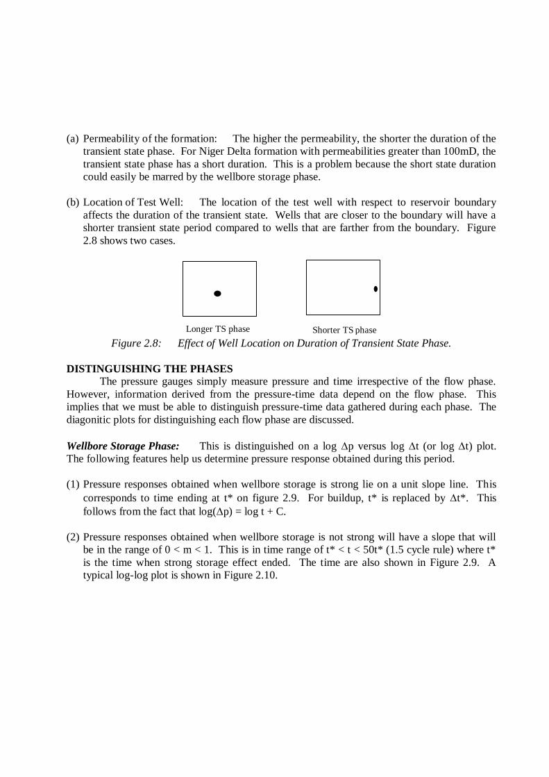
(a) Permeability of the formation: The higher the permeability, the shorter the duration of the
transient state phase. For Niger Delta formation with permeabilities greater than 100mD, the
transient state phase has a short duration. This is a problem because the short state duration
could easily be marred by the wellbore storage phase.
(b) Location of Test Well: The location of the test well with respect to reservoir boundary
affects the duration of the transient state. Wells that are closer to the boundary will have a
shorter transient state period compared to wells that are farther from the boundary. Figure
2.8 shows two cases.
Longer TS phase Shorter TS phase Figure 2.8: Effect of Well Location on Duration of Transient State Phase.
DISTINGUISHING THE PHASES The pressure gauges simply measure pressure and time irrespective of the flow phase.
However, information derived from the pressure-time data depend on the flow phase. This
implies that we must be able to distinguish pressure-time data gathered during each phase. The
diagonitic plots for distinguishing each flow phase are discussed.
Wellbore Storage Phase: This is distinguished on a log p versus log t (or log t) plot.
The following features help us determine pressure response obtained during this period.
(1) Pressure responses obtained when wellbore storage is strong lie on a unit slope line. This
corresponds to time ending at t* on figure 2.9. For buildup, t* is replaced by t*. This
follows from the fact that log(p) = log t + C.
(2) Pressure responses obtained when wellbore storage is not strong will have a slope that will
be in the range of 0 < m < 1. This is in time range of t* < t < 50t* (1.5 cycle rule) where t*
is the time when strong storage effect ended. The time are also shown in Figure 2.9. A
typical log-log plot is shown in Figure 2.10.

Wellbore Storage
Transient Late Time
timet* 50t* t esl
(Figure not to scale)
Figure 2.9: Phases and Duration of Wellbore Storage Phase.
)45
50t* Time t (or t)
p
t*
Figure 2.10: Log-log plot.
Parameters in the graph are defined as follows:
p = pi - pwf (Drawdown)
p = pws - pwf (tp) (Buildup)
t = flowing time (drawdown)
t = shut-in time (Buildup)
pi = initial pressure
pwf = flowing pressure
tp = total flowing time
pwf(tp) = flowing pressure at shut-in time
pws = shut-in pressure.

The wellbore storage phase can easily be distinguished on a derivative plot. On this plot
the wellbore storage phase forms clearly defined “hump” as shown in Fig.2.11.
Derivative
Wellbore Storage Hump
45
Time
Fig. 2.11: Derivative Plot - Diagnostic Plot for Wellbore Storage Phase
Since the advent of the derivative plot, I have always relied on it when detecting pressure
responses affected by wellbore storage phase. In most cases, both the pressure and derivative
plots are displayed in one graph. This is shown in Figure 2.12.
Derivative
and Pressure
Wellbore Storage Hump
45
Time
Fig. 2.12: Log-log Plot of Pressure and Derivative.
Pressure
Derivative
Transient State Phase: Pressure responses obtained during the good transient state phase
will fall on a straight line when pressure is plotted against log of time (semilog plot). The time
in this case is defined as follows:
time = flowing time for drawdown
time = shut-in time for buildup (mDH Plot)

time = t t
t
p
for buildup (Horner Plot)
This follows from the fact that p = m[ log t(ime) + C].
The semilog plots are shown in Figure 2.13, 2.14 and 2.15.
Pwf
50t*Log t
Figure 2.13: Semilog Plot-Drawdown Test.
Log t50t*
Pws
Figure 2.14: MDH Plot - Buildup Test.

Pws
Stabilizing at
average pressure
1log
tp t
t
Figure 2.15: Horner Plot - Buildup Test.
The good transient state phase is the transient state not influenced by wellbore storage
phase. It occurs in the time range 50t* < t < tesl. The term tesl is the time when transient ends
and it is shown in Figure 2.9.
The good transient state phase can also be clearly discerned on a derivative plot. The
derivative plot in this case falls on a horizontal line after the end of the wellbore storage hump.
This is shown in Figures 2.11 and 2.12. Figure 2.16 shows factors that affect buildup test.
Late Time Phase: The diagonistic plot for the late time phase depends on the nature of the
outer boundary. We shall not go in detail, but a summary of the different plots are as follows:
(a) For wells with closed outer boundaries, plots of flowing pressure versus time during the late
time phase fall on a straight line if Cartesian graph paper is used. The slope of the straight
line is related to the drainage volume of the well.
(b) For a well in a closed system that is shut-in, the pressure buildup to average pressure during
the late time phase.
The derivative plots for the different boundary conditions are shown in Figure 2.17.
3. BASIS OF ANALYZING BOTTOM HOLE TESTS
In this section, we shall discuss some concepts that form the basis for analyzing bottom-hole
pressure tests. The concepts include the following:

1. Graphical presentation of Data
2. Units and conversions
3. Flow phases and identification
4. Flow geometry
5. Typical models
3.1 Graphical Presentation of Data
Graphs are one of the preferred methods for presenting information and yet they are often poorly
made. In welltesting, many graphs of bottom-hole pressure versus time are used to deduce
desired information. In this section, we shall discuss how to make good graphs and common
types of graphs used in welltest analysis.
3.1.1 Making Good Graphs
To make a good graph involves the following:
(a) Correct Labelling: The axis of the graph must be correctly labelled with units. For
example, time (hr); pressure ( psi); Dimensionless pressure, etc.
(b) Proper Scaling: Choosing the scale of a graph is important. The scales should be chosen
such that unnecessary subdivision of the grids in the graph paper is avoided. It is convenient to
choose the grid spacing such that each unit represents 1, 2, 5, 10, etc.
(c) Data Points: Data points on any graph should be made conspicuous using symbols such as
, , , etc. The practice of representing data points with dots should be discontinued because
once a line passes through such points, the position of the point may be obscure. We are more
interested in the points and not in the line. In addition, each data set should be represented using
the same type of symbol. Different data sets should be represented with different symbols.
(d) Title of Graph: Every graph must have a title, which briefly explains what the graph is all
about. It is now common practice to put the title at the bottom of the graph. In some cases, some
information may be put on the graph in the form of legend or something to make the graph
understandable.
3.1.2 Types of Graphs
The three common graphs used in well testing are the Cartesian, semilog and log-log graphs.
The Cartesian, semilog and log-log graphs are included as Specimen A, B and C respectively.
Further discussion on these graphs follows:
Leave 3 pages for the specimens ????


(a) Cartesian Graph Paper: This is used for graphing data set (x,y) of the form
y = a + m x 3.1
Equation 3.1 is simply the equation of a straight line where “a” is the intercept while “m” is the
gradient (slope). The intercept is the value of y when x = 0 while the gradient is calculated as
change in y (y) divided by change in x (x). The units of the intercept a, and gradient m are
a = intercept (units of y) and m = gradient unitsof y
unitsof x.
(b) Semilog Graph Paper: This is used for graphing data set (x,y) of the form
y = a + m log x 3.2
The advantage of using the semilog graph for plotting data set that satisfy Eq. 3.2 is that on the
semilog paper, the abscissa (x-axis) is already in log scales. Hence the data points can just be
plotted without finding the logarithm of x. From Eq. 3.2, it can be shown that the value of “a”
corresponds to the value of y when x is equal to one. This follows from the fact that log 1 is
zero. The gradient m, in Eq. 3.2 is defined as
m = change in y per cycle of x
Mathematically,
12
12
loglog xx
yym
Generally, x2 and x1 are chosen so that they are one cycle apart. In that case, the denominator is
unity.
The major grids on a log scale are scaled to the powers of ten. That is, 10-2, 10-1, 10o, 101, 102,
etc. The interval between 10x and 10x+ 1, where x is an integer is known as a cycle. Note that a
data set that satisfied Eq. 3.2 may still be graphed on a Cartesian graph to obtain a straight line.
In that case, the transformation
X = log x 3.3
is required. Hence the final equation becomes:
y = a + m X 3.4

(c) Log-log Graph Paper: This type of graph is used for data set of the form:
log y = a + m log x 3.5
The gradient m, in Eq. 3.5 is given in cycles of y per cycle of x. The gradient may be calculated
using the equation:
m = 12
12
xlog - xlog
y log - y log 3.6
The points (x1, y1) and (x2, y2) are taken arbitrarily from the straight line. The log-log graph
paper is already divided into log scales and the data points are graphed directly without finding
the logarithm of anything. By suitable transformation, the data set that satisfy Eq. 3.6 may be
graphed on a Cartesian graph to get a straight line but the slope of the straight line will be
different from that obtained from Eq 3.5.
3.2 SYMBOLS, UNITS AND CONVERSIONS
In this section, we shall discuss symbols, units and unit conversions.
a) Symbols and Units
The three unit systems used in welltesting are the CGS, Oilfield and SI units. Although the
Oilfield units are more common, but the preferred unit is the SI unit. Some of the welltest
parameters, symbols and units are shown in Table 3.1. For more symbols and units, refer to SPE
Metric Standard (1982). We assumed that you are already familiar with basic definitions of
reservoir properties.
Table 3.1: Symbols and Units
Parameter Symbol CGS Units Oilfield Units Practical S.I. Units
Liquid Flow Rate q cc/sec STB/day m3/day Permeability k Darcy millidarcy
(mD)
millidarcy (mD)
Time t seconds (s) hours (hr) seconds (s) Liquid Viscosity centipoise centipoise millipascal-second
Compressibility c atm-1 psi-1 kpa-1 Wellbore Storage Cs cc/atm bbl/psi m3/kpa
Porosity fraction of bulk volume same as CGS same as CGS
Saturation S fraction of pore volume same as CGS same as CGS
Pressure p atm psi kpa
Thickness h cm ft m
Skin Effect s dimensionless dimensionless dimensionless
b) Conversion Factors
Some basic conversion factors used in this welltesting are as follows:
1 atmosphere (atm) = 14.7 psi = 1.01325 x 10⁵ kpa
1 cp = 1 x 10⁻⁶ kpa-s
1 barrel (bbl) = 1.589873 x 10⁻¹ m3
1 bb1/day = 1.840131 x 10⁻⁶ m3/s
= 1.840131 cc/s
More conversion factors are given in Table 3.2 taken from Earlougher (1977).
Leave two pages for conversion factors ??????
TABLE 3.2-CONVERSION FACTORS USEFUL IN WELL TEST ANALYSIS.
SI conversions are in boldface type. All quantities are current to SI standards as of 1974. An
asterisk (*) after the sixth decimal indicated the conversion factor is exact and all following
digits are zero. All other conversion factors have been rounded. The notation E + 03 is used in
place of 103, and so on.


c) Unit Conversion
The Society of Petroleum Engineers (SPE) recommends the use of S.I. units. Articles that appear
in SPE journals are now written using both the SI units and the Oilfield units. The Oilfield units
are also referred to as English units.
Conversion from one set of units to another is easy. Two cases will be discussed here. The first
case considers conversion of a quantity expressed in one unit to another unit. The second case
considers conversion of an equation with parameters expressed in some units to an equivalent
equation with parameters given in different units. In both cases, what is required is a conversion
factor. Consideration for given cases follows:
Case 1: Conversion of a given quantity from one unit to another
Example 1 (a) ft inches
3ft = 3ft x 12 inches
ft1
old conversion
units factor
(first)
= 36 inches
Example 2
bb1 ft3
5 bb1 = 5 bb1 x 5.614583
b b l ft3 ( 5.61 x 5) ft3
Note that in both cases, if the units in the numerator and denominator are cancelled, the resultant
unit (unit to remain uncancelled) is the new unit.
Case 2: Conversion of units in an equation
Example 1
q = K A p
L
3.7
Equation 3.7 is the steady state form of Darcy’s law for a linear system. The parameters in Eq.
3.7 are in Darcy’s units.

That is:
q ccS
k (D) A (cm) p (atm)
(cp) L (cm)( ) =
3.8
Equation 3.8 can be converted to Oilfield units. That is:
q (cc
S) q (
STB
day)
k (D) k (mD)
A (cm2) A (ft2)
p (atm) p (psi)
(cp) (cp)
L (cm L (ft)
Note that while the flowrate in Darcy’s units is expressed at reservoir conditions, in Oilfield
units, it is expressed at stock tank conditions. Conversion of Eq. 3.8 to Oilfield units is done by
replacing all terms in the original equation (Eq 3.8) with other terms and combining to get the
overall conversion factor. The terms in Eq. 3.8 and their replacements are as follows:
Parameters in Original Equation Replacements
k (D) K (mD) x 1 (D)
1000 (mD)
A (cm2) A (ft2) x 30.48 (cm
(
2 )
1 ft )2
p (atm) p (psi) x 1
14 7
( )
. ( )
atm
psi
(cp) (cp)

L (cm) L (ft) x 30.48 (cm)
1 (ft)
q(cc/s) q (STB/day) Bobbl
STB x
1 day
(24x3600)sec
158987.3 cm
1 (bbl)
3
x
Substituting,
q (STB
day x B (
bbl
STB x
1 day
(24 x 3600) secso) ) x 0.158973m
bbl x
100 cm
m
3 3 3
3
= k(mD) x D
1000mD x A(ft ) x
(30.48) cm
ft
) x 30.48cm
ft
22 2
2
(cp) L (ft
x p (psi) x (atm)
. psi
3.9
Evaluating, Eq. 3.9 becomes
qB STB
day x 1.84013 = 0.002073469
k (mD) A (ft p (psi)
(cp) L (ft)
2
o
)
3.10
and therefore,
q (STBday
x 10 K(mD) A(ft p (psi)
(cp) B (bbl)
(STB) L(ft)
-32
o
) .)
. 3.11
The conversion factor 1.127 x 10⁻³ should be familiar to those who have taken basic reservoir
engineering courses.
Example 2
Dimensionless pressure is defined in Darcy’s unit as:
PD =
q
P] - [P 2 ikh 3.12

The term PD in Eq. 3.12 may for now be considered to be just a dimensionless number
(pressure). Equation 3.12 is in Darcy’s unit. That is:
PD (dimensionless) =
)((S)
(cc)q
(atm) p (cm)h (D) 2
cp
k
3.13
Conversion of Eq. 3.13 to Oilfield units is done as follows:
PD (dimensionless) = 2k(mD) x ( ).481
1000
30D
mDh ft x
cm
ftx
x
p psi psi
qSTB
dayx B
bbl
STBx
day
x s
x
o
atm
14.7
( ) ( )( )sec24 3600
01589873 106 3. x cm
bblx cp 3.14
PD (dimensionless) = 2 x 0.0011268 K mD h ft p psi
qSTB
dayB
bbl
STBcpo
( ( )
( )
= kh p
q Bo
141 2. 3.15
This implies that dimensionless pressure, defined in Darcy’s unit as
PD = 2
kh p
q
, 3.12
is given in oilfield units as
PD = kh p
qBo
141 2. 3.16
Similarly, it can be shown that dimensionless time tD is defined in Darcy’s units as:
tD = kt
c rt w 2 3.17
is given in Oilfield units as
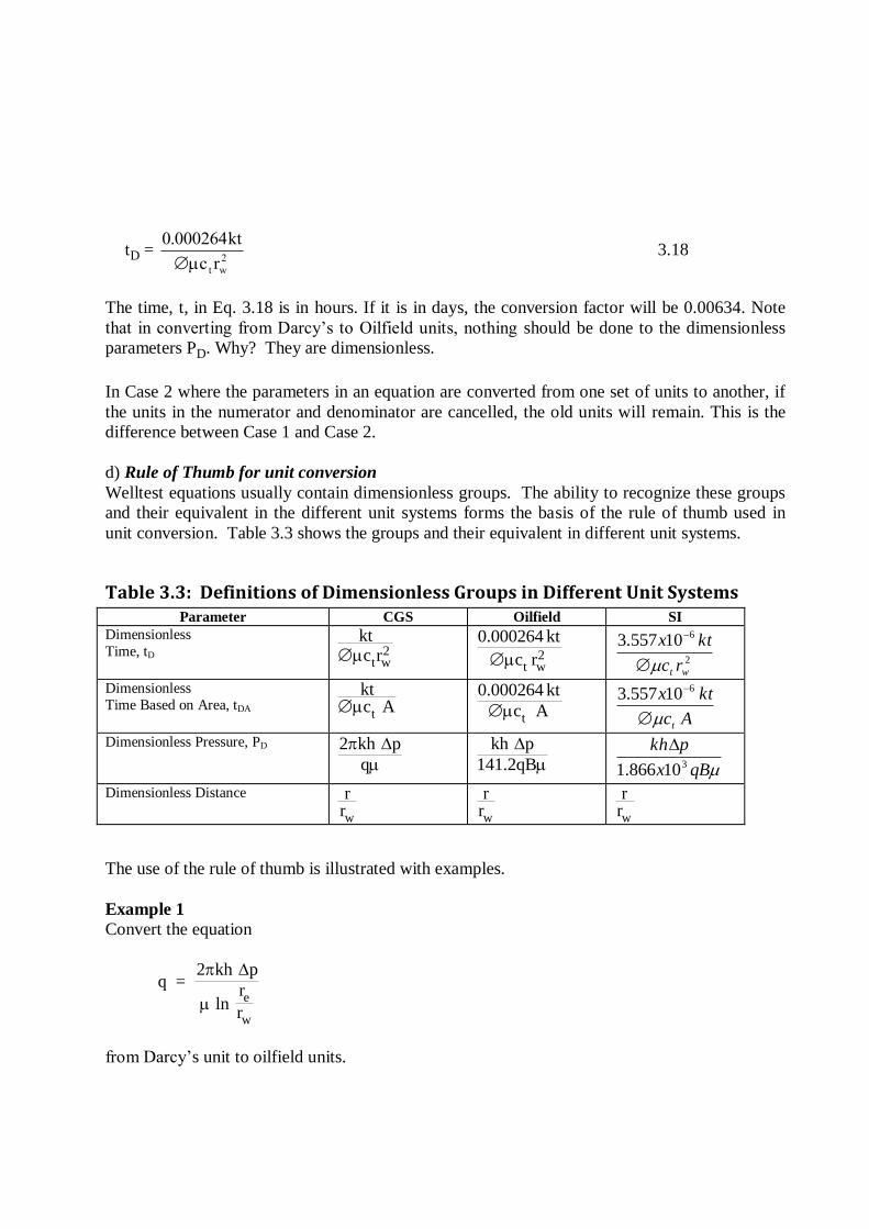
tD = 0 000264
2
. kt
c rt w 3.18
The time, t, in Eq. 3.18 is in hours. If it is in days, the conversion factor will be 0.00634. Note
that in converting from Darcy’s to Oilfield units, nothing should be done to the dimensionless
parameters PD. Why? They are dimensionless.
In Case 2 where the parameters in an equation are converted from one set of units to another, if
the units in the numerator and denominator are cancelled, the old units will remain. This is the
difference between Case 1 and Case 2.
d) Rule of Thumb for unit conversion
Welltest equations usually contain dimensionless groups. The ability to recognize these groups
and their equivalent in the different unit systems forms the basis of the rule of thumb used in
unit conversion. Table 3.3 shows the groups and their equivalent in different unit systems.
Table 3.3: Definitions of Dimensionless Groups in Different Unit Systems Parameter CGS Oilfield SI
Dimensionless
Time, tD ktc rt w 2
0.0002642
kt
c rt w
2
610557.3
wt rc
ktx
Dimensionless
Time Based on Area, tDA ktc At
0.000264 kt
c At
Ac
ktx
t
610557.3
Dimensionless Pressure, PD 2
kh p
q
kh p
141.2qB
qBx
pkh310866.1
Dimensionless Distance rrw
r
rw
rrw
The use of the rule of thumb is illustrated with examples.
Example 1
Convert the equation
q = 2
kh p
r
re
w
ln
from Darcy’s unit to oilfield units.

Solution
Rearrange the equation into recognizable dimensionless groups as follows
ln r
r
kh p
qe
w
2
(Form of Dimensionless Distance) (Dimension Pressure)
Therefore, the equation in oilfield unit is
ln r
r
kh p
qBe
w
141.2
Rearranging
q = 7.08 10 3x kh p
Br
re
w
ln
Example 2
Convert the following equation in Darcy’s unit to Oilfield unit.
P = pi + )4
(4
2
kt
rcE
kh
q t
i
Solution
Rearranging to bring out the dimensionless group,
2 x 2
4
2
kh p p
qE
c r
kti
i
t
Recognizable dimensionless groups and their oilfield equivalents are as follows
2
141.2qB
kh p p
q
kh p pi i
c r
kt
c r
ktt t
2 2
0.000264
Substituting, the oilfield equivalent of the equation is

2
141.2qB 4x0.000264
2kh p pE
c r
kti
it
making “p” the subject gives
p = pi + 70.6qB
0.001056
2
khE
c r
ktit
3.3 Dimensionless Forms Many dimensionless parameters are defined in petroleum engineering. The dimensionless
parameters make it possible to cast fluid flow equations into dimensionless forms. The
advantages and disadvantages of the dimensionless forms are given in this section. Also, the
definitions of some of the dimensionless parameters are given.
a). Advantages of Dimensionless Forms (i) Ease of comparing solutions
(ii) Makes it possible for results to be generalized.
For example, the pressure at any point in a single well reservoir produced at constant rate q, is
written in a general form using dimensionless pressure as:
Pi - P(r, t) = 1412.
, , ,qB
kh
[P (t r C geometry ) + s]D D D D 3.19
Equation 3.19 is in Oilfield units and the dimensionless pressure, PD, is a function of other
dimensionless parameters, rD, tD and CD.
(iii) With pressure expressed in dimensionless form, It becomes easier to apply superposition
concept to handle varying flowrates and pressure drop in multiwell systems.
(iv) Dimensionless form aid in presentation of results in a more compact form. Also, the
results are invariant in form, irrespective of the unit system used.
b) Disadvantages of Dimensionless Forms (i) With dimensionless form, the engineer may loose a sense of magnitude of the quantity.
For example, a time of 24 hours may correspond to dimensionless time of 300 for a tight
reservoir and a dimensionless time of 1000 for a highly permeable sand. This follows from the
way dimensionless parameters are defined.

3.3.1 Definition of Dimensionless Parameters In Darcy Units
Dimensionless Time
t D = kt
c rt w
2 3.20
Dimensionless Time Based on Area
t D A
t
= kt
c A 3.21
Dimensionless Radius
rD = r
rw
3.22
Dimensionless Pressure
PD = 2 kh
q (P - P (r, t) )i
3.23
PD = P - P (r, t)
P - P
i
i wf
3.24
The form of dimensionless pressure, PD, used in any problem depends on the type of boundary
condition used at the well. Use Eq 3.23 if well produces at constant pressure and Eq 3.24 for
well producing at constant rate.
Dimensionless Cumulative Production
q D = q (t)
2 kh (P - Pi wf
)
QD
o
tDW
= q dtD DW 3.25
Other Dimensionless Parameter
kt
c r rt D r =
kt
c r
r =
t2
t w
2
w
2
D
2 2 3.26

3.4 FLOW PHASES
Just like a man goes through phases in life, a well undergoing a test also passes through phases
with each phase revealing some information about the well or reservoir. It is therefore necessary
that we understand the phases and how to identify them to avoid problem of obtaining required
information from a wrong phase.
In this section, we shall describe the phase and methods of diagonizing the phases.
3.4.1. Flow Phases in Drawdown and Buildup Tests Figure 3.1 shows the phases that a well undergoes during a drawdown or buildup test. In case,
there is a wllbore storage phase, transient phase and late-time phase. The late-time phase
depends on the nature of the boundary and test (drawdown or buildup).
Wellbore Storage
A B C D E
Transient State Phase Late-Time Phase
Increasing Flow Time
Figure 3.1: Flow Phases in Buildup or Drawdown Test.
Some deductions from Fig 3.1 are as follows:
1. The wellbore storage phase is an independent phase and can occur concurrently with the
transient state. This happened in Interval BC.
2. The wellbore storage phase with no concurrent transient phase is known as the “strong
wellbore storage”. This is represented by Interval AB.
3. If wellbore storage and transient state occur concurrently, the pressure-time data acquired
will be “polluted” and cannot be analyzed using conventional method of analysis.
4. The wellbore storage phase may last so long that all the transient state phase may be
“polluted”. Tests must be designed so that this type of “pollution” does not occur as the
most valuable information from such tests are obtained from the unpolluted transient state
phase.
5. The transient state phase without concurrent wellbore storage phase is the “good transient
state phase”. This is represented by Interval CD.
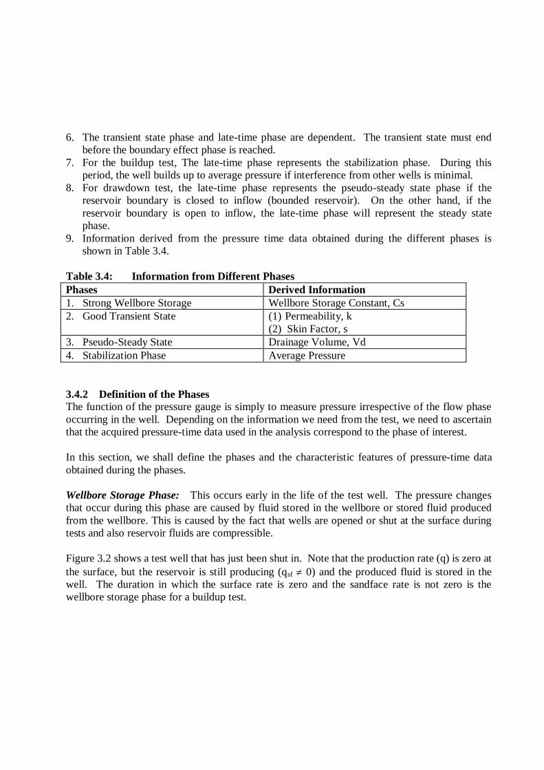
6. The transient state phase and late-time phase are dependent. The transient state must end
before the boundary effect phase is reached.
7. For the buildup test, The late-time phase represents the stabilization phase. During this
period, the well builds up to average pressure if interference from other wells is minimal.
8. For drawdown test, the late-time phase represents the pseudo-steady state phase if the
reservoir boundary is closed to inflow (bounded reservoir). On the other hand, if the
reservoir boundary is open to inflow, the late-time phase will represent the steady state
phase.
9. Information derived from the pressure time data obtained during the different phases is
shown in Table 3.4.
Table 3.4: Information from Different Phases
Phases Derived Information
1. Strong Wellbore Storage Wellbore Storage Constant, Cs
2. Good Transient State (1) Permeability, k
(2) Skin Factor, s
3. Pseudo-Steady State Drainage Volume, Vd
4. Stabilization Phase Average Pressure
3.4.2 Definition of the Phases The function of the pressure gauge is simply to measure pressure irrespective of the flow phase
occurring in the well. Depending on the information we need from the test, we need to ascertain
that the acquired pressure-time data used in the analysis correspond to the phase of interest.
In this section, we shall define the phases and the characteristic features of pressure-time data
obtained during the phases.
Wellbore Storage Phase: This occurs early in the life of the test well. The pressure changes
that occur during this phase are caused by fluid stored in the wellbore or stored fluid produced
from the wellbore. This is caused by the fact that wells are opened or shut at the surface during
tests and also reservoir fluids are compressible.
Figure 3.2 shows a test well that has just been shut in. Note that the production rate (q) is zero at
the surface, but the reservoir is still producing (qsf 0) and the produced fluid is stored in the
well. The duration in which the surface rate is zero and the sandface rate is not zero is the
wellbore storage phase for a buildup test.

q = 0 q = 0
qsf = 0qsf ‡ 0
Wellbore Storage
phaseEnd of wellbore Storage
phaseIncreasing Shut-in time
Figure 3.2: Surface and Reservoir Production During Shut-in.
Figure 3.3 shows wellbore storage phase in a drawdown test. In this case, on opening the well
for a drawdown test, the initially produced fluid is the fluid stored in the wellbore. Thai is, q =
qwb. Wellbore storage phase ends in this case when the total production is equal to the fluid
produced by the reservoir. That is, q = qsf.

q = qwb + qsfq = qsf
qsf = q
qwb = 0
qsf = 0
or
qsf < q
Wellbore Storage
phaseEnd of wellbore Storage
phase
Increasing production time0
qwb
Figure 3.3: Surface, Wellbore, and Reservoir Production in an Opened Well.
In Figure 3.3, qwb is the production from fluid stored in the well. Note that if qsf = 0 for
drawdown or qsf = q in a shut-in well, we have strong a wellbore storage phase. The manner in
which q, qsf and qwb vary during buildup and drawdown tests are shown in Figure 3.4.
q = qsf + qwb
q
0 time ts tete
qwb
qsf
qsf
Drawdown Buildup
Wellbore
storage
Wellbore
storage
Figure 3.4: Rate Variation During Buildup and Drawdown Tests.

In Figure 3.4,
te = end of wellbore storage phase for drawdown test
ts = shut-in time
te = End of wellbore storage phase for buildup test.
The wellbore storage phase is a nuisance because it “pollutes” the transient phase from which
we can get useful information about our reservoir. The duration of the well storage phase must
be reduced or eliminated if it is possible.
To reduce the duration of wellbore storage phase will require knowledge of the factors that can
affect the phase. The factors are mainly compressibilty of the wellbore fluid and wellbore
volume.
(a) The compressibility of the fluid in the well: The higher the compressibility of the fluid, the
longer the duration of the wellbore storage phase. The compressibility of the wellbore fluid
depends on the gas-oil ratio (GOR). Wells with high GOR has high wellbore fluid
compressibility . Can the GOR be reduced?
(b) The volume of the well that communicate with the tubing: This is shown by the volume of
the shaded region in Fig. 3.5. Figure 3.5a represents a case with a packer while Fig 3.5b
represents a case without a packer or a non-sealing packer. The duration of the wellbore
storage phase increase with the increase in volume communicating with the tubing.
(c) Production Rate: The production rate of the well also affects the duration of the wellbore
storage phase. The higher the production rate, the smaller the duration of the wellbore
storage phase.
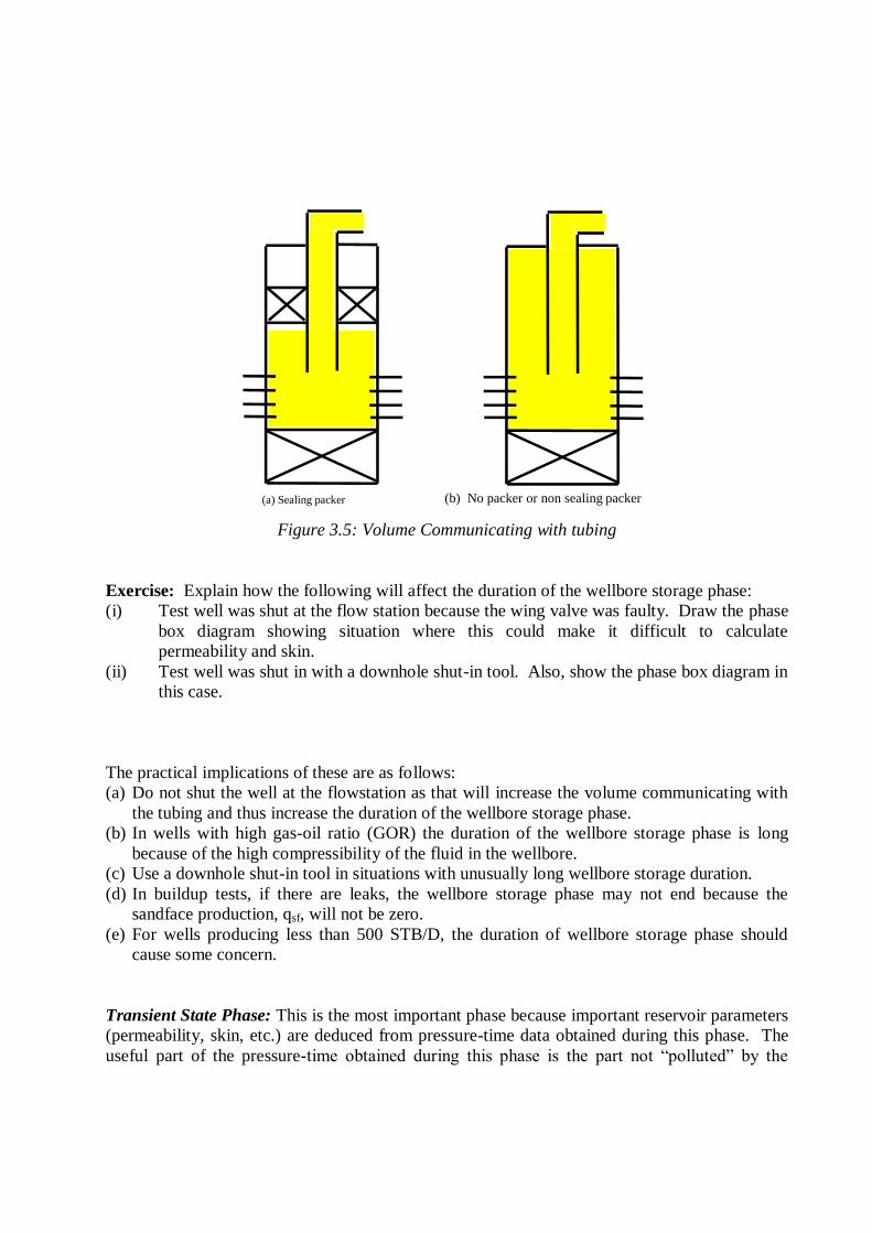
(a) Sealing packer (b) No packer or non sealing packer
Figure 3.5: Volume Communicating with tubing
Exercise: Explain how the following will affect the duration of the wellbore storage phase:
(i) Test well was shut at the flow station because the wing valve was faulty. Draw the phase
box diagram showing situation where this could make it difficult to calculate
permeability and skin.
(ii) Test well was shut in with a downhole shut-in tool. Also, show the phase box diagram in
this case.
The practical implications of these are as follows:
(a) Do not shut the well at the flowstation as that will increase the volume communicating with
the tubing and thus increase the duration of the wellbore storage phase.
(b) In wells with high gas-oil ratio (GOR) the duration of the wellbore storage phase is long
because of the high compressibility of the fluid in the wellbore.
(c) Use a downhole shut-in tool in situations with unusually long wellbore storage duration.
(d) In buildup tests, if there are leaks, the wellbore storage phase may not end because the
sandface production, qsf, will not be zero.
(e) For wells producing less than 500 STB/D, the duration of wellbore storage phase should
cause some concern.
Transient State Phase: This is the most important phase because important reservoir parameters
(permeability, skin, etc.) are deduced from pressure-time data obtained during this phase. The
useful part of the pressure-time obtained during this phase is the part not “polluted” by the

wellbore storage phase. Due to the usefulness of this phase, the following guidelines must be
followed during tests.
(1) Design and run test so that not all parts of the transient state phase will be “polluted” by the
well bore storage phase.
(2) Test duration must be such that the transient state phase must be reached before the test is
stopped.
The transient state phase occur when the pressure changes at the wells are not influenced by the
nature of the boundary. For example, if you drop a little stone into a bowl containing water,
concentric waves will move outwards as shown in Figure 3.6.
Figure 3.6: Waves illustrating Transient State Period.
The waves will continue to move outwards until they hit the side of the bowl. The waves get
distorted and become less orderly. The period during which the waves have not hit the boundary
can be likened to transient state phase because the effect of the boundary has not been felt. The
mathematicians describe this phase as period when the rate of pressure change with time is
neither zero or constant. All systems go through the transient state irrespective of the nature of
the boundaries.
The duration of the transient state is affected by many factors which includes the following:
(a) Permeability of the Formation: The higher the permeability, the shorter the duration of the
transient state phase (waves move faster). For Niger Delta formation with permeabilities
greater than 1000 mD, the transient state phase has a short duration. This is a problem
because the short transient state duration could easily be marred by the wellbore storage
phase.
(b) Location of Test Well: The location of the test well with respect to reservoir boundary
affects the duration of the transient state. Wells that are closer to the boundary will have a
shorter transient state period compared to wells that are farther from the boundary. Figure
3.7 shows two cases.

Longer TS phase Shorter TS phase Figure 3.7: Effect of Well Location on Duration of Transient State Phase.
Late-Time Phase: The nature of the late-time phase depends on nature of test. For buildup
test, the well will build up to average pressure at late-time if there is just one well in the
reservoir. In case where we have many wells, the well will build up and then drops due to
interference effect. In a situation where the drainage area of the test well is large, the pressure
may build up to average pressure before dropping. The pressure profile in such case is shown in
Fig 3.8.
For drawdown, the nature of the late-time phase depends on the type of the outer boundary
condition of the reservoir. If the boundary is open to inflow (water influx), a steady state will be
attained during the late-time phase. During steady state, pressure in the system will no longer be
changing with time. If the reservoir boundary is closed to flow, a pseudo-steady state will be
attained at late time. During the pseudo-steady state period, pressure in the system will be
changing, but the rate at which the pressure will be changing everywhere in the system will be
constant. The value of the is related to the drainage volume of the test well and this is the basis
of reservoir limit test. Figure 3.9 shows the transient state, steady state and pseudo-steady state
phases during a drawdown test.
Shut in Pressure
Shut in Time
No Interference
Interference
Fig. 3.8: Effect of Interference
Transient
Steady State
Pseudo-Steady State
Log (Flowing Time)
Pwf

For steady state to be attained there must be an adjoining aquifer providing the source of water
influx and the aquifer permeability must be large to permit ease of flow of water into the
reservoir. Reservoirs in highly faulted environment are more likely to be sealed off and less
likely to be in contact with such an aquifer.
3.5 Flow Geometry
Depending on the reservoir and nature of perforations in well, flow could occur linearly,
radially, spherically or elliptically. In some cases, the flow geometry could change with time
from one form to another. In this section, we shall discuss equations governing the different
flow geometries and parameters that may be deduced from the flow geometry.
3.5.1 Linear Flow
The plan and elevation in situations where linear flow occur is shown in Figure 3.10
Plan Elevation
Fig. 3.10: Linear Flow Geometry
The linear flow described here is the one-directional flow that occurs in Cartesian co-ordinates.
The practical situations where linear flow could in a reservoir are as follows:
a. Single Vertical Fracture Intersecting Well
This case is illustrated in Figure 3.11. The permeability in the fracture zone is much greater than
the permeability of the formation (infinite conductivity). Therefore, fluid flows linearly into the
fracture and the wellbore. Such flow occurs at early time and will explained later.
Fig 3.9: Transient, Steady and Pseudo-Steady States

Fig 3.11: Vertically Fractured Well
Linear flow is also observed at early time in situations where the flow per unit area of fracture is
constant (uniform flux fracture).
b. Horizontal Well
At some period, linear flow could occur in horizontal wells. The flow streamlines in a
horizontal well during linear flow is shown in Figure 3.12.
?????????????? Cut and paste
Fig. 3.12: Linear Flow in Horizontal Wells
c. Reservoirs with Strong Partial Influx
In a reservoir where a segment is open to strong water influx, flow will be dominant in the
direction of the influx. Depending on the size of segment, the flow to the wellbore could be
linear.
In situations where linear flow occur, the flow could be modelled with the equation:
2
2x
ctk t
------------------------------------------------------------------- 3.27
Equation 3.27 is also a diffusivity equation. Hence, all assumptions relating to diffusivity
equation will hold.
The solution to Equation 3.27 is of the form
p = (At)½ -------------------------------------------------------------------------- 3.28
Taking log of both sides,
Reservoir
Boundary
Well
Fracture
xf
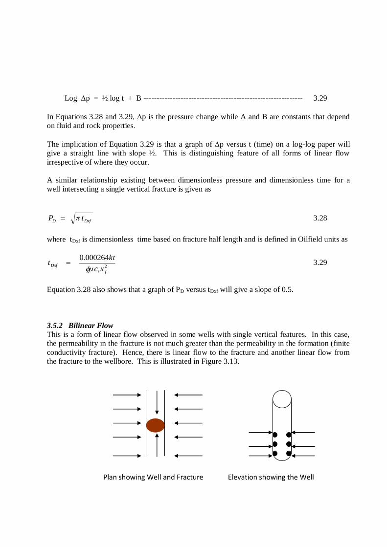
Log p = ½ log t + B ------------------------------------------------------------ 3.29
In Equations 3.28 and 3.29, p is the pressure change while A and B are constants that depend
on fluid and rock properties.
The implication of Equation 3.29 is that a graph of p versus t (time) on a log-log paper will
give a straight line with slope ½. This is distinguishing feature of all forms of linear flow
irrespective of where they occur.
A similar relationship existing between dimensionless pressure and dimensionless time for a
well intersecting a single vertical fracture is given as
DxfD tP 3.28
where tDxf is dimensionless time based on fracture half length and is defined in Oilfield units as
2
000264.0
ft
Dxfxc
ktt
3.29
Equation 3.28 also shows that a graph of PD versus tDxf will give a slope of 0.5.
3.5.2 Bilinear Flow
This is a form of linear flow observed in some wells with single vertical features. In this case,
the permeability in the fracture is not much greater than the permeability in the formation (finite
conductivity fracture). Hence, there is linear flow to the fracture and another linear flow from
the fracture to the wellbore. This is illustrated in Figure 3.13.
Plan showing Well and Fracture Elevation showing the Well

Fig. 3.13: Bilinear Flow Geometry
For the bilinear flow, the relationship between pressure change and time is
p = A t¼
--------------------------------------------------------------------------- 3.30
Taking log,
Log p = ¼ log t + B ----------------------------------------------------------- 3.31
Equation 3.31 implies that a graph of p versus t (time) on a log-log graph has a unique
slope of ¼.
3.5.3 Radial Flow
This is the most common flow geometry and occurs when the flowing fluid surrounds the
wellbore and flow streamlines come from distances that are large compared to the size of the
wellbore. Streamlines converge towards a central point in each plane. Figure 3.14 shows the
plan and elevation during radial flow.
Plan showing Well and Streamlines Elevation showing Well and Strealines
Fig 3.14: Radial Flow
Irrespective of what it is called (pseudo-radial, late-time radial, early-time radial, etc.) the
relationship between pressure and time in all forms of radial flow is
p = A log t + B ---------------------------------------------------------------- 3.32

In Figure 3.14, p is pressure change, (Pi – p), t is time (or some form of time function), and A
and B are constants that depend on the reservoir characteristics.
The implication of Equation 3.32 is that a graph of p (or pressure) versus log t gives a straight
line. This is shown in Figure 3.15 for a drawdown test.
Fig. 3.15: Semilog Straight line Due to Radial Flow
Radial flow could occur virtually in all system including horizontal well. In a reservoir with a
single vertical fracture, a form of radial flow, pseudo-radial flow, occurs at the end of the linear
flow. Figure 3.16 shows the pseudo-radial flow occurring in a system with a single vertical
fracture.
Fig 3.16: Pseudo-radial Flow occurring in well with a Single Vertical Fracture
In Fig 3.16, the streamlines come from far distances and the fracture behaves as a point source.
A form of radial flow (pseudo-radial) also occurs in horizontal wells and this is shown in Figure
3.17.
???????????? cut and paste
0.1 1 10 100 1000
2000
2500
3000
Pressure
Time

Fig 3.17: Pseudo-radial Flow occurring in Horizontal Well
A form of radial flow, hemiradial flow, occurs when the well is close to a boundary as shown in
Fig. 3.18. Equation 3.32 also holds for a hemiradial flow with constants, A and B defined
appropriately.
Fig 3.18: Hemiradial Flow
3.5.4 Spherical Flow
For this case, flow occurs from all directions towards the wellbore. This is shown in Figure
3.19.
Plan Elevation
Fig 3.19: Spherical Flow
Spherical flow could occur in thick reservoirs if the perforated interval is small. Moran and
Finklea (1962) used spherical flow equations for analysing pressure transient data. Raghavan
(1975) found an expression for vertical permeability in a partially penetrating well using
spherical flow equations.
Boundary

The spherical flow equations at early and long times are of the forms:
Early Time
p = At1/2
------------------------------------------------------- 3.33
Long Time
p = 1 - 1
12Bt
------------------------------------------------- 3.34
In Equations 3.33 and 3.34, A and B are constants. Graphical implications of Equations 3.33
and 3.34 are obvious. Onyekonwu and Horne (1983) published detail on the equations.
Equation 3.34 is generally recognized as the spherical flow equation and hence a plot of pressure
versus the inverse of the square root of time yields a straight line.
3.6 Flow Geometry and Phases
In this section, we illustrate using box diagrams the phases and geometries that occur during
transient in some well and reservoir systems.
a) System with Wellbore Storage and Skin in Homogeneous Reservoir
Fig. 3.20: Radial Flow in a Homogeneous Reservoir
b) System with Well on a Single Vertical Fracture
Wellbore Storage Phase
Radial Flow
Transient State Phase Late-Time Phase
Increasing Time
Wellbore Storage Phase
Transient State Phase Late-Time Phase
Increasing Time
Linear Flow Pseudo-Radial Flow
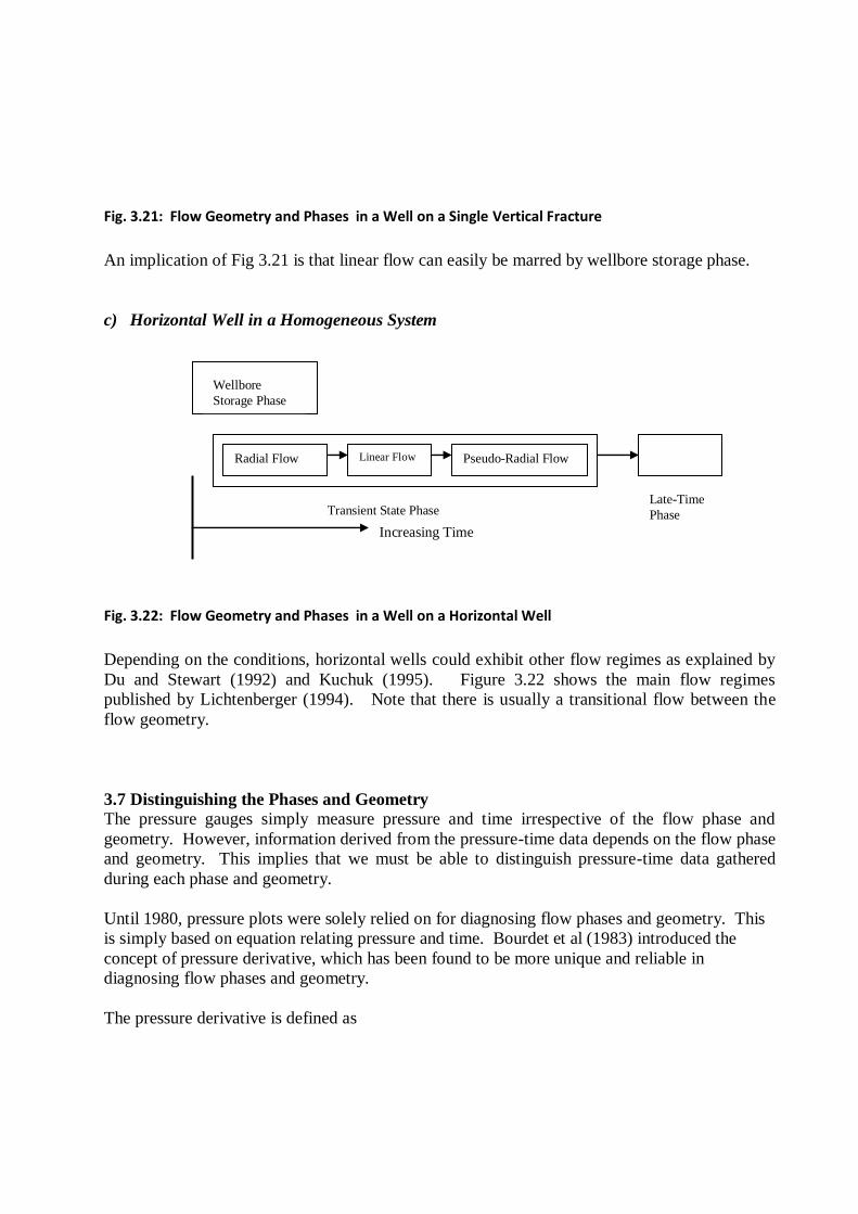
Fig. 3.21: Flow Geometry and Phases in a Well on a Single Vertical Fracture
An implication of Fig 3.21 is that linear flow can easily be marred by wellbore storage phase.
c) Horizontal Well in a Homogeneous System
Fig. 3.22: Flow Geometry and Phases in a Well on a Horizontal Well
Depending on the conditions, horizontal wells could exhibit other flow regimes as explained by
Du and Stewart (1992) and Kuchuk (1995). Figure 3.22 shows the main flow regimes
published by Lichtenberger (1994). Note that there is usually a transitional flow between the
flow geometry.
3.7 Distinguishing the Phases and Geometry The pressure gauges simply measure pressure and time irrespective of the flow phase and
geometry. However, information derived from the pressure-time data depends on the flow phase
and geometry. This implies that we must be able to distinguish pressure-time data gathered
during each phase and geometry.
Until 1980, pressure plots were solely relied on for diagnosing flow phases and geometry. This
is simply based on equation relating pressure and time. Bourdet et al (1983) introduced the
concept of pressure derivative, which has been found to be more unique and reliable in
diagnosing flow phases and geometry.
The pressure derivative is defined as
Wellbore
Storage Phase
Transient State Phase Late-Time
Phase
Increasing Time
Linear Flow Pseudo-Radial Flow Radial Flow

))(( tfdIn
dpP 3.35
where f(t) is a time function which may be defined as follows:
f(t) = t (drawdown test)
f(t) = t (buildup test)
f(t) = (tp + t)/t (buildup test)
The derivative of pressure drop could also be used and in that case, the pressure term in Eq. 3.35
is replaced with p.
As pressure values during test are obtained at discrete times, the pressure derivative is obtained
numerically. Horne (1990) published an algorithm that can be used in obtaining the derivative
as follows:
ii t
pt
t
p
ln 3.36
=
kijiiji
jikii
tttt
ptt
/ln/ln
/ln+
kiiiji
iikiji
tttt
pttt
/ln/ln
/ln 2
-
kijikii
kiiji
tttt
ptt
/ln/ln
/ln 3.37
In Eq. 3.36 and 3.37, the time function is assumed to be time. The constraints on the time in Eq.
3.37 are as follows:
In ti+j - In ti 0.2 and In ti - In t i-k 0.2
The value of 0.2 (known as differentiation interval) could be replaced by smaller of larger values
(usually between 0.1 and 0.5), with consequent differences in the smoothing of the noise in the
pressure data. Higher values yield a more smoothened derivative.
Pressure derivatives characteristic shapes published by Gringarten (1987) are shown in Fig.
3.23.
????? leave 3 inches
Fig 3.23: Characteristic Shapes of Pressure Derivatives
Table 3.5 summarizes the feature and the characteristics of the derivative

Table 3.5: Features and Characteristics of the Derivatives
Features Characteristics of Derivative
Wellbore storage and skin Hump with derivative attaining a maximum
Stimulated or fractured well No hump, No maximum
Heterogeneous behaviour A “valley”
Fault Upward turn
Closed boundary (drawdown) Upward turn
Closed boundary (buildup) Downward turn
Constant pressure
(due to influx or gas-cap)
Downward turn
Infinite-acting radial flow (IARF) “flat” (zero gradient)
Linear Flow Gradient with slope of 0.5
Spherical flow Gradient with slope of - 0.5
Strong wellbore storage Gradient with slope of 1 (unity)
Hemiradial flow “flat” (zero gradient at a higher level)
Table 3.5 will form the basis for using pressure derivative for diagnosis.
3.7.1 Diagnostic Plots for Distinguishing Flow Phases
In this section, we shall show the diagnostic features of the phases using pressure (or pressure
drop) and pressure derivative. Discussion now follows:
Diagnosing Wellbore Storage Phase: Wellbore storage is distinguished on a log p versus log t
(or log t) plot. The following features help us determine pressure response obtained during this
phase.
(1) Pressure responses obtained when wellbore storage is strong lie on a unit slope line. This
corresponds to time ending at t* on Figure 3.24. This follows from the fact that
log(p) = log t + C. 3.38
For buildup, t* is replaced by t*.
(2) Pressure responses obtained when wellbore storage is not strong will have a slope that is in
the range of 0 < m < 1. The duration of this part of wellbore storage phase is in time range
of 10t* < tewb< 50t* (1 to 1.5 cycle rule) where t* is the time when strong storage effect
ended. The times are shown in Figure 3.24.
(3) A typical log-log plot is shown in Figure 3.25.

Wellbore Storage
Transient Late Time
timet* t esl
(Figure not to scale)
tewb
Figure 3.24: Phases and Duration of Wellbore Storage Phase.
Figure 3.25: Log-log Showing Wellbore Storage Influenced Data
Parameters in Figure 3.25 are defined as follows:
p = Pi - pwf (Drawdown)
p = Pws - pwf (tp) (Buildup)
0.1 1 10 100
Time, t or Shut-in Time, t
1
10
100
p
45o
t* tewb

t = flowing time (drawdown)
t = shut-in time (Buildup)
Pi = initial pressure
pwf = flowing pressure
tp = total flowing time
pwf(tp) = flowing pressure at shut-in time
Pws = shut-in pressure.
The wellbore storage phase is more easily distinguished on a log-log plot of the pressure
derivative. On this plot the wellbore storage phase forms clearly defined “hump” as shown in
Fig.3.26.
Derivative
Wellbore Storage Hump
45
Time
Fig. 3.26: Derivative Plot - Diagnostic Plot for Wellbore Storage Phase
Since the advent of the derivative plot, I have always relied on it when detecting pressure
responses affected by wellbore storage phase. In most cases, both the pressure and derivative
plots are displayed in one graph. This is shown in Figure 3.27.

Derivative
and Pressure
Wellbore Storage Hump
45
Time
Fig. 3.27: Log-log Plot of Pressure and Derivative.
Pressure
Derivative
Diagnosing Transient State Radial FlowPhase: Pressure responses obtained during the good
transient state radial flow phase or infinite-acting radial flow phase (IARF) will fall on a straight
line when pressure is plotted against log of time (semilog plot). The time in this case is defined
as follows:
time = flowing time for drawdown
time = shut-in time for buildup (MDH Plot)
time = t t
t
p
for buildup (Horner Plot)
This follows from the fact that during the good transient,
p = A + m[ log t(ime) + C]. 3.39
where A and C are constants. Also, m is a constant that depends on fluid and rock properties.
The semilog plots are shown in Figure 3.28, 3.29 and 3.30.
Log (time)
Pwf
tewb

Figure 3.28: Semilog Plot (Drawdown Test)
Good
Transient
Log t
Pws
Good
Transient
Log (t +t/t) 1
Pws
Stabilizing
at average
pressure
Fig. 3.29: Horner Plot

Fig 3.30: MDH Plot
The good transient state phase is the transient state not influenced by wellbore storage phase. It
occurs in the time range tewb < t < tesl. The term tesl is the time when transient ends and it is
shown in Figure 3.24.
Many factors affect the semilog straight line obtained during the transient state phase. Figure
3.31 taken from Mathews and Russell (1967) show how these factors affect the semilog straight
line.
????? ask for fig 3.31.

The good transient state phase can also be clearly discerned on a derivative plot. The derivative
plot in this case falls on a horizontal line (“flat”) after the end of the wellbore storage hump.
This is shown in Figures 3.32.
Fig 3.32: Flow Phases Discerned on Pressure Derivative
Transient state is more uniquely identified on a dimensionless pressure-time plot. A graph of
dimensionless pressure versus log of dimensionless time has a unique slope with a value of
1.151. This is shown in Fig 3.33.
Derivative
Logp
Log (time)
m= 1.151
Log tD
PD
Wellbore Storage
dominated Good Transient
Wellbore
Storage Phase
Transient
State Phase
Pressure
Unit slope line

Fig 3.33: Dimensionless Plot Showing Transient State
The unique slope follows from the fact that
PD = 1.151 [log tD + C] 3.40
Equations that can be used for diagnosing other flow geometries during the transient state have
been discussed under flow geometries.
Diagnosing Late Time Phase: The diagnostic plot for the late time phase depends on the nature
of the outer boundary and the type of test. We shall not go in detail, but a summary of the
different plots is as follows:
Drawdown Test (Closed Boundaries): For drawdown test in wells with closed outer boundaries,
the system attains pseudo-steady state at late time. Cartesian plots of flowing pressure versus
time during the late time phase yields a straight line. The slope of the straight line is related to
the drainage volume of the well. Figure 3.34 shows the diagnostic plot.
Fig. 3.34: Cartesian Plot Showing Pseudo-Steady State
Time
Wellbore storage
and transient state
phases Pseudo-steady state
Flowing
Pressure
Slope = m

The basis of the plot shown in Fig 3.34 follows from the equation that holds during pseudo-
steady state:
Pwf = A + mt 3.41
Where A and m are constants. The value of m is related to the drainage volume and this forms
the basis of reservoir limit test.
The dimensionless plot is a more unique plot for detecting pseudo-steady state because a graph
of dimensionless pressure versus dimensionless time based on area has a slope of 2 during
pseudo-steady state. Figure 3.35 shows the dimensionless plot.
Fig. 3.35: Dimensionless Plot Showing Pseudo-Steady State
The basis of Fig 3.35 is Eq 3.42 which is as follows:
PD = 2tDA + C 3.42
Where C is a constant.
Drawdown Test (Open Boundaries): For a drawdown test with boundaries open to flow, the
system will attain steady state (pressure remains constant) if the influx through the boundaries is
sufficient to stop further pressure decline.
A semilog graph for systems with closed boundaries and constant pressure boundaries is shown
in Fig 3.36.
Slope = 2
Pseudo-steady state
PD
Dimensionless Time based on Area, tDA

Fig. 3.36: Semilog Plot of Drawdown Data with Different Boundary Conditions
Pseudo-steady state
Wellbore storage Transient Late-time
Log (time)
Steady state
Pwf

Buildup Test: For a well in a closed system that is shut-in, the pressure builds up to average
pressure during the late time phase. If there are many wells in the system, pressure in the test
well will build up and later drop due to interference effect. If there is a large gas-cap, the system
attains a constant pressure due to the gas-cap.
The derivative plots for the different late-time conditions are discussed in Chapter 4.
10. BOTTOM-HOLE PRESSURE TESTS IN HORIZONTAL WELLS The objectives of bottom-hole pressure tests in vertical and horizontal wells are similar. Actually, a horizontal well
can be viewed as a vertical well with infinite conductivity vertical fracture or a highly stimulated vertical well.
However, BHP tests in horizontal wells are more difficult to analyze for the following reasons.
1. The horizontal wells are not perfectly horizontal as assumed by the analysis models. The
wells may be snake-like as shown in Fig. 10.1.
Fig. 10.1 Snake-Like Nature of some Horizontal Wells
The consequence of the snake-like nature of horizontal wells is that waves emanating from different sections of the
horizontal well at the same time may hit different boundaries. This complicates pressure response.
2. The total drilled length may not all contribute to the producing length. Some drilled length may intersect
non-productive interval. The unknown non-producing length is erroneously accounted for as skin factor.
3. There are many possible flow regimes which depending on the reservoir and well conditions may or may not
be properly discerned from pressure tests.
In this chapter, we shall present basic information about horizontal wells and how to identify the
flow regimes obtained during horizontal welltests. We shall also present flow equations and how
to analyze horizontal welltests.
10.1 Introduction A horizontal well is a well drilled parallel to the reservoir bedding plane while a vertical well is drilled
perpendicular to the reservoir plane. This is shown in Fig 10.2. With horizontal well, we can enhance reservoir
Vertical
Depth
Horizontal Distance

contact by well and therefore hence enhance well productivity. This implies that the drainage area of the horizontal
well is bigger than that of a vertical well. Joshi (1988) showed two methods of calculating the drainage area of
horizontal well based on knowledge of the drainage area of a vertical well. Joshi’s procedures are presented.
Fig. 10.2: Vertical and Horizontal Wells.
Drainage Area of Horizontal Well
If the drainage area of a vertical well is
A = rev2
10.1
Where rev is shown in Fig 10.3.
Fig. 10.3: Drainage Area of Vertical Well
The two method for the calculating the drainage area of horizontal well are as follows:
Horizontal Well Vertical Well
rev

Method 1: This assumes that each end of the horizontal well drains a semi-circle drainage area while the length
drains a rectangular drainage area as shown in Fig 10.4.
rev
Fig. 10.4: Rectangular/Semi-Circle Drainage Area
Assuming that h rev,
HWDA = rev2 + L 2rev 10.2
Where
HwDA = Drainage area of the horizontal well
L = Productive length of the horizontal well
Method 2: We assume an elliptical drainage area in the horizontal plane, with each end of a well
as a foci of drainage ellipse as shown in Fig 10.5.
Fig. 10.5: Elliptical Drainage Area
In this case, the drainage area is,
HWDA = ab 10.3
where
L
L

a = half major axis of ellipse = L
2 + rev
b = half minor axis = rev
The calculated drainage areas (using different methods) are not the same. Therefore, the average
of the two can be used as the effective drainage area.
Applications of Horizontal Wells (a) Some naturally fractured reservoirs
(b) Reservoir with gas/water coning problems
(c) Thin reservoirs
(d) Reservoirs with high vertical permeability
(e) In EOR projects with injectivity problems
(f) In fields (e.g. offshore) requiring limited wells due to cost or environmental problems.
Advantages of Horizontal Wells (a) Horizontal well productivities are 2 to 5 times greater than that of unstimulated vertical well. Actually, the
performance of horizontal wells depends on the effective length of the horizontal section in the formation.
Higher productivity may result to early payout.
(b) Horizontal well may intersect several fractures or compactments and help drain them effectively
(c) Reduce coning tendencies
(d) As injectors can improve sweep efficiency in EOR projects
Disadvantages of Horizontal Wells (a) Ineffective in thick (500ft to 600ft) low permeability reservoirs.
(b) Cannot easily drain different layers
(c) Technological limitations
(d) Cost more (1.4 to 2 times) than cost of drilling a vertical well.
Dimensionless Parameters used in Horizontal Wells Dimensionless parameters are also used in horizontal wells. Figure 10.6 shows dimensions and coordinates in
horizontal wells.
h
x
z
y
zw
L/2

Fig. 10.6: Dimensions in a Horizontal Wells
Table 10.1 shows the different dimensionless parameters in Darcy unit.
Table 10.1: Dimensionless Parameters used in Horizontal Wells
Dimensionless Parameters Equations
Dimensionless Pressure in terms of h and kr PDh = k h p
Br
s o o
141.2q
Dimensionless Pressure in terms of L and k kr z PDL = k h L p
Br z
s o o
141.2q
Dimensionless Time in terms of L/2 tD = 0.0002637k
2)2r
t
t
c (L /
Dimensionless Time in terms of h and kz tDz = 0.0002637k
2z
o t
t
c h
Dimensionless Time in terms of ye and ky tDy =
0.0002637k
2
y
o t e
t
c y
Dimensionless Time in terms of h and ye tDhy = 0.0002637ky
o t
t
c hye
Dimensionless Time in terms of and rw tDrw = 0.0002637
2
k k t
c rr z
o t w
Derivative in terms of pDL
pdp
d tDLDL
D
'
ln
Derivative in terms of pDh
pdp
d tDhDh
D
'
ln
Dimensionless x, y, z Coordinate xD = 2(x-xw)/L yD = 2(y-yw)/L zD = z/h
Dimensionless Wellbore Location
xwD = 2xw/xe
ywD = 2yw/ye

zwD = zw/h
Dimensionless x, y-direction boundary width xeD = 2xe/L
yeDL = 2ye/L
Dimensionless Wellbore Length
LD = L k
kz
r2h
Dimensionless Wellbore Radius rwD = 2rw/L
10.2. Flow Regimes During BHP Tests In Horizontal Wells
During bottom-hole pressure tests in a horizontal well, the followoing flow regimes could be
discerned: linear, radial, hemiradial, and pseudo-radial. Figure 10.7 is a box diagram showing
some of the flow regimes and the order in which they occurred.
Some parameters in Table 5.1 are defined as follows:
Zw = vertical distance measured from bottom of payzone to the well
Xw, Yw, Zw = Well location co-ordinates
Xe, Ye = reservoir boundaries in x and y directions
L = Length of horizontal well
kr = kh = permeability in horizontal place
= k kx y
kz = kv = vertical permeability
Fig. 10.7: Typical Flow Regimes in a Horizontal Well
The pressure and pressure derivative for the case shown in Fig 10.7 is shown in Fig 10.8 taken
from Lichtenberger (1994).
Transient State
Wellbore Storage
Radial Linear Pseudoradial Boundary Effect

Fig. 10.8: Pressure and Derivative for a Typical Horizontal Well BHP Test
Details on the flow regimes are as follows:
Early Radial Flow: Figure 10.9 shows the early time radial flow period in a vertical plane, which develops, when
the well is put initially on production. The well acts as though it is a vertical well turned sideways in a laterally
infinite reservoir with thickness, L. This flow period ends when the effect of the top or bottom boundary is felt or
when flow across the well tip affects pressure response. This flow regime may not develop (Kuchuk , 1995) if the
anisotropic ratio, kH/kV is large.
Fig. 10.9: Early Radial Flow in a Horizontal Well
Many authors (Ozkan et al, 1989; Goode and Thambynayagam, 1987; Odeh and Babu, 1990; Du
and Stewart, 1992; Lichtenberger, 1994 and Kuchuk, 1995) published equations for identifying
the different flow regimes. Inferences from their publication show that the early radial flow can
be identified using the pressure derivative or semilog plot if it is not marred by wellbore storage
effects. The pressure derivative gives a zero slope as shown in Fig 10.8 while a graph of
pressure versus log of time yields a straight line. The basis for the straight line is the equation

Pi - pwf =
As
rc
kk
Lkk
qB
wt
vy
yv
87.023.3 t
log
6.1622
10.4
where s = skin due to damage/stimulation. If it is positive, it is denoted as Sm, mechanical damage due to drilling
and completion.
Also, A is a constant given by Lichtenberger (1994) as
A = 2.303 log ½ k
k
y
v
4 + k
k
v
y
4
10.5
The equation implies that a graph of Pwf versus log t gives a straight line with slope
m1 = 162 6. qB
k kv y
L
10.6
From this, the equivalent permeability in the vertical plane, k kv y , can be calculated.
k km L
v y = qB162 6
1
.
10.7
The skin equation for the first radial flow period is
S = 1.151 Pi
r
- P 1 hr
m - log
k k
c + A + 3.23
1
y v
t w2
10.8
Note:
1. In arealy isotropic reservoir, kx = ky = kh
2. If effective reservoir permeability k kv y is known, the given equation can be used in determining the
effective producing length.
3. The early-time flow regime can be short and may be completely marred by wellbore storage effect. Use of
downhole shut-in tool is useful here. Time to end of wellbore storage is given by Lichtenberger (1994) as:
/
)2404000(
Lkk
Cst
vh
mEus
10.9
where
tEus = time for end of wellbore storage effects, hours

sm = skin factor
C = wellbore storage constant, rb/psi
L = effective producing length of well, ft
= viscosity of oil, cp
kh = horizontal permeability = yxkk
kv,kx,ky = permeability in the vertical, x and y directions respectively.
Early radial flow ends when either of the following will occur:
a. Effect of bottom or top boundary is felt.
b. Flow across well tips affects pressure response
Mathematically, different authors gave time to the end of early radial flow, te1, as follows:
Goode and Thambynayam (1987)
te1 =
v
wz
k
d t
095.0095.2 c r 190
10.10
where dz is the distance of the well to the closest boundary (top or bottom)
Odeh and Babu (1990) and Licthenberger (1994)
te1 = min
d C
k
C
k
z2
t
v
t
y
1800
125 2
L
10.11
The first equation represents the time when the effect of the boundary (top or bottom) will
distort early radial flow while the second equation represents time when flow across the tip of
the well will distort early radial. Lichtenberger assumed areal isotropy in his equations.
DU and Stewart (1992)
te1 = min
C d
k
C d
k
t z2
v
t x2
x
947
947
10.12
where dx is nearest distance from well point to the boundary normal to the well length axis. Other parameters are as
defined earlier.

Although the equations by different authors are not exactly the same, but they are similar and therefore can be used
as a guide.
Hemiradial Flow : When the wellbore is closer to any of the no-flow boundaries, hemi-radial (or hemi-elliptical)
flow may develop. This produces slope doubling on the semilog plot and p1 (pressure derivatives) will plateau at twice the radial flow value.
The flow equation during the hemi-radial flow period is given by Kuchuk (1995) and Lichetenberger (1994) as
Pwf = Pi - 2 x162 6
3 230 87
22
.log .
.qB
k k
k k
c r
SA
H v
H v
t w
L
t
10.13
where
A = log
w
z
r
d
v
H
k
k + 1
dz = distance to the nearest boundary (top or bottom)
Lichtenberger (1994) gave the time for the end of the hemiradial flow as
tEhrf = 1800 d c
k
z2
t
v
10.14
Implications of the Eq 10.13 are as follows:
a. A plot of pwf versus log t is a straight line with slope m
b. k kmL
H v = 2 qB162 6.
10.15
c. The skin equation is
S = 2.30
w
zi
r
d
r
P
V
H
2
wt
vH
k
k+1log + 3.23+
c
kklog -
m
hr 1P -
10.16
Intermediate Linear Flow: This flow regime may develop after the effects of upper and lower boundaries are felt at
the well. Figure 10.10 shows the streamlines during the intermediate-time linear flow. This flow regime develops
if the well length is sufficiently long compared with reservoir thickness and there is no constant pressure boundary.

Fig. 10.10: Intermediate Linear Flow
The flow equation during the linear flow is given as follows:
Pi - Pwf = 8128. qB
Lh
t
c kS S
t y
z
+
141.2 qB
L k ky v
10.17
where SZ is the pseudo-skin factor caused by partial penetration in the vertical direction and is given by different
authors as:
Odeh and Babu (1990)
SZ = lnh
rw
+ 0.25 ln
k
k
Z
h
y
v
wln sin .180
1838
10.18
Lichtenberger (1994)
SZ
h
d s i n 1
h zw
y
v
k
kr
10.19
Kuchuk (1995)
SZ = ln
h
d sin
k
k + 1
h
w
H
vw r
10.20
Implications of the flow equations are as follows:
a. A graph of (Pi -Pwf) versus t is a straight line
b. Slope of line

m2 = 8128. qB
Lh c kt y
10.21
Therefore
L2 ky = 8128
2
2
. qB
hm ct
10.22
c. p t o
y v
zL k k
S S
= 141.2 qB
10.23
where pt=0 is the pressure drop at time equals zero. The skin due to damage, S, can therefore be calculated as SZ is known (calculated from Equation 10.18, 10.19 or 10.20)
Time to end of early linear flow is given by different authors as follows:
Goode and Thambynayagam (1987)
te2 = 20 8. c L
k
t2
x
10.24
Du and Stewart (1992)
te2 = 16 c L
k
t2
x
10.25
Odeh and Babu (1990) and Lichtenberger (1994)
te2 = 160 c L
k
t2
x
10.26
Odeh and Babu (1990) also gave the time to the start of early linear flow period as
tS2 = 180 D c
k
z2
t
v
10.27
where Dz (= h-dz) is the maximum distance between the well and the z-boundaries (top or bottom boundary)
Pseudoradial Flow: In sufficiently large reservoir, pseudo radial flow will develop eventually as the dimensions of
the drainage areain the horizontal plane becomes much larger that the effective well length. Figure 10.11 is a

schematic showing the streamlines during the pseudoradial flow. This is similar to what happens in a horizontal
with a vertical fracture.
Fig 10.11: Pseudoradial Flow
The flow equation during the pseudoradial flow period is given as follows:
Pi – Pwf = SSkkL
qBA
Lc
tk
kk
qBZ
vyt
x
yx
2.141log
h
6.1622
10.28
where “A” is a contant given by many authors as follows:
A = 2.023 (Goode and Thambynayagam, 1987)
A = 2.5267 (Kuchuk, 1995)
A = 1.76 (Odeh and Babu, 1990) A = 1.83 (Lichtenberger, 1994
Implications of Eq 10.28 are as follows:
a. Graph of Pwf versus log t is a straight line
b. Slope,
m3 = 162 6. qB
k hx
ky
10.29
Therefore
k kqB
m hx y
162 6
3
.
The skin equation is
S = 1151 1
32
.log
L
h
k
k
Pi P hr
m
k
c LA Sv
x
x
t
Z
Note:

a. Pseudo radial develops if L>>h (hD 2.5) b. If top or bottom boundary is maintained at constant pressure, no pseudo-radial flow period will occur.
Instead, there is steady state flow at late time.
Time for beginning of pseudoradial flow, ts3, is given by different authors as follows:
tS3 = 1230 L c
k
2t
x
(Goode and Thambynayagam
tS3 = 1480 L c
k
2t
x
(Odeh and Babu, Lichtenberger used 1500)
tS3 = 2841 c L
k
t2
x
(Du and Stewart)
Lichtenberger (1994) gave the time for the end of the pseudoradial flow as follows:
tEprf = min
1650
2000 4
2
2
C D
k
C L D
k
t x
H
t w y
H
/
10.30
where Dx and Dy are the lateral distances of the reservoir in the x and y directions respectively.
Late Linear Flow Period: After, the pseudoradial flow, it is possible that a late-time linear flow period develops.
The flow equation for this phase is
Pi - Pwf = 8128
2
. qB
x
t
k cS
eh y t
x
+
141.2qB
L k k + S + S
y v
z
10.31
where
2xe = width of reservoir
Sx = pseudo skin due to partial penetration in the x direction.
Implications of Eq 10.31 are obvious.
Skin in Horizontal Well The skin factor will serve the same purpose in horizontal well as it does in vertical wells. The dominant pseudoskins
in horizontal wells are the pseudoskin due to damage and pseudoskin due to convergence in the z-direction. The
pseudoskin due to damage is dominant because of more fluid losses resulting from larger area contacted by the well.
The pressure loss due to skin is defined with respect to the formation thickness in vertical wells and well length in
horizontal wells. This is shown in the following equations:

Pressure loss due to skin in vertical wells:
pqB
khs vertical S
1412.
10.32
Pressure loss due to skin in horizontal wells:
pqB
kLs Horizontal
S
1412.
10.33
From Eqs 10.32 and 10.33, we infer that the pressure loss due to skin in horizontal well is much smaller than the
pressure loss due to skin in vertical wells because the horizontal well length is usually longer than the formation thickness.
The small pressure loss due to skin in horizontal wells does not imply that skin has small effect
on horizontal well productivity because the drawdown in horizontal wells is also small. The
remedial factor, R, used in vertical wells should also be used in horizontal wells to quantify the
effect of skin.
Problem Set
A 2100ft long well is completed in a 100 ft thick formation with closed top and bottom boundaries. The estimated
average horizontal permeability from several vertical well test is 1500md while the vertical permeability is 300md.
The horizontal well has a diameter of 8½ in and is located 30ft from top of the sand. Other parameters are as follows:
= 20%, = 0.65cp, ct = 20 x 10-6psi-1 and s = 5. Also, assume dx = L/2
(a) Assuming that the early radial flow will not be distorted by wellbore storage effects, determine the time when
the early radial flow will end. Also, determine when wellbore storage effect will end if wellbore storage
constant, c = 0.025 rb/psi.
(b) Calculate the time to start and end of the early linear flow period for the horizontal well whose parameters
have been given
(c) For given reservoir and well data, calculate time required to start a pseudo-radial flow.
(d) Using the following additional data calculate the pressure change in a horizontal well. S = 25, q =
4000 STB/D and Bo = 1.05 rb/STB
Tabulated Solution to Problem
Authors
End of early
radial flow
tel x10-3 (hrs)
End of well-
bore storage
effect tews x10-5 (hrs)
Start of early
linear flow
ts2 x10-3 (hrs)
End of
early
linear flow te2(hrs)
Start of
Pseudo
Radial Flow ts3 (hrs)
Skin due to
partial pent.
In vert. dir. Sz
P @ the start of Pseudo
Radial flow
P (psi)
Goode et al 2.560 N/A N/A 0.159 9.402 N/A N/A
Odeh and Babu 14.040 N/A 7.644 1.223 11.313 3.996 12.11

Du and Stewart 7.387 N/A N/A 0.122 21.717 N/A N/A
Lichtenberger N/A 5.998 N/A N/A 11.466 2.15 x 10⁻⁴ 10.833
N/A implies author did not give required equation
10.3 Detecting Flow Regimes Using Pressure Derivative
The pressure derivative is the best diagnostic tool for detecting flow regimes. This follows from
the characteristic slopes of the derivatives obtained for different flow regimes on a log-log plot.
Figure 10.12 shows the characteristic slope for the first radial, hemiradial and pseudoradial flow
regimes in a horizontal well. Note that the derivatives have zero slopes at different levels. For
linear flow, the derivative has a slope of 0.5.
Log
Log (time)
Fig 10.12: Prssure Derivatives for the Different Radial Flow Regimes
Figure 10.13 taken from Kucuk (1995) shows the pressure derivative for cases with well and reservoir parameters
shown in Table 10.2.
Fig 10.13 : Derivatives for Cases Shown in Table 10.2
Table 10.2: Reservoir Parameters for Examples Shown in Fig 10.13
Example h, ft kH, md KV, md Lw, ft zw, ft rwD
Pressure
Derivative
Early Radial
Hemiradial
pseudoradial

1 100 100 10 500 20 0.00146
2 100 100 1 500 20 0.00389
3 100 100 5 500 5 0.00194
4 40 100 5 500 20 0.00197
5 200 200 1 500 20 0.00530
V
H
w
wwD
k
k
L
rr 1
2
Deductions from the derivatives are as follows:
(a) The first radial period can be seen in all cases. (b) In Example 3, the well is close to the boundary (5ft) and therefore, hemiradial flow occurred after a short
duration early radial flow. (c) In Example 4, a linear flow regime manifested because the well length is much greater than formation
thickness
(d) In all cases, the pseudoradial flow developed
Du and Stewart (1992) quantified the effect of parameters on the flow regimes. In their work,
they defined dimensionless parameters as follows:
PDL = 2
k kpz r L
q.
10.34
PDL1
= dp
d ln t
DL
DZ
(Pressure Derivative)
10.35
tDZ = kz t
c ht2
10.36
Values of PDL1
for different flow regimes are as follows:
PDL1
= 0.5 vertical radial flow
PDL1
= 1 vertical hemi-radial flow
PDL1
= LD pseudo radial flow
Du and Stewart (1992) concluded that parameters zWD (dimensionless well location in the z-direction) and LD (dimensionless wellbore length) have the dominant effect on flow regimes obtained in horizontal wells. These
parameters are defined as follows:
zwD = zw/h and
H
vD
k
k
h
LL
2

Figure 10.14 shows effect of LD on flow regimes for infinite reservoir with no flow top and bottom. Horizontal well
is in the center of the formation (ZWD = 0.5).
Fig. 10.14: Effect of LD in Homogeneous Laterally Infinite Reservoir With Sealed Top and Bottom
Inferences from Fig. 10.14 are as follows:
(i) For LD 3 the flow regimes are: Vertical radial flow (VRF; PDL1
= 0.5) + transition + early linear flow
opposite the completed section (ELF; Gradient = ½ ) + transient reservoir pseudo radial flow (PRF; PDL1
=
LD).
(ii) For LD < 3, the flow regimes are: VRF + vertical spherical flow (VSF;)
Gradient = - ½ + transition + PRF. The smaller LD, the longer the duration of VSF.
(iii) The smaller the LD, the shorter the duration of VRF and longer the length of PRF.
(iv) For LD 0.1, no VRF at all. For a 100ft thick formation and Kz / Kr = 0.2, this implies a minimum well length of 45ft.
Figure 10.15 shows effect of ZWD. From Fig 10.15, we infer that when ZWD 0.1 (well close to one of the boundaries), there is a hemi-radial flow (HRF), between VRF and ELF with a transition in between.
Figure 10.16 shows the effect of ZWD in a situation with gas cap. The dimensionless well length, LD, is large.

Fig. 10.15: Effect of ZwD in Homogeneous Laterally Infinite Reservoir With Sealed Top and Bottom
Fig. 10.16: Effect of ZwD in Homogeneous Laterally Infinite Reservoir With Bottom Constant Pressure
Boundary and Top No Flow Boundary
Inferences from the graph are as follows:
(i) When ZWD < 0.5 (well closer to the bottom no-flow boundary) the flow regimes are as follow: VRF +
transition + HRF + transition + constant pressure effect (rollover).
(ii) When ZWD 0.5 (well nearer the constant pressure boundary) the flow regimes are VRF + transition + rollover (constant pressure effect).
(iii) The nearer the well to the constant pressure boundary, the stronger the constant pressure boundary effect.
The effect of the boundaries is similar to what obtains in a vertical well. A no - flow boundary
causes stabilization at higher level with respect to the infinite reservoir case. Figure 10.17
shows the effect of lateral boundaries, which are parallel to the direction of well length.

Fig. 10.17: Effect of Lateral Boundaries in Reservoir With Sealed Top and Bottom
10.4 Field Cases
In this section, we shall discuss some field examples of bottom-hole pressure tests. The
objective is to see what may actually obtain in real life. Table 10.3 shows basic parameters or
the different tests.
Table 10.3: Parameters for Different Field Cases
Parameters Values for Different Cases
1 2 3 4
Formation thickness, ft 73 95 19 123
Well length, ft 1984 1387 232 1330
Well location, ft 7 7.4 8 16.1
Oil rate STB/D 3948 4144 685 4951
Porosity, % 29 29 24 29
Oil Viscosity, cp 1.97 1.97 0.34 2.23
Formation volume factor, rb/STB 1.128 1.120 1.539 1.298
Wellbore radus, ft 0.4 0.4 0.4 0.3
Calculated Permeability, md 15363 16320 1070 3820
Calculated Skin 35 23 0 -1.4
Drawdown, psi 15 10 9 34
Discussions on the field cases follow:
Case 1: Figure 10.18 shows the pressure and pressure derivative for this case.

Fig. 10.18: Pressure and Pressure Derivative for Case 1
The pressure derivative shows wellbore storage, early vertical radial flow, early linear flow, hemiradial flow and
“rollover” due to a constant pressure boundary. The hemiradial flow was inferred because of the nearness of the
well to the bottom boundary and the fact that p (VRF) 2p (HRF). The constant pressure effect was caused by gas-cap. Figure 10.18 shows that mathematical models give us good insight unto pressure and flow regime obtained
during actual BHP tests.
Case 2: Figure 10.19 shows pressure data for Case 2. Case 2 and Case 1 are from the same reservoir in western Niger Delta. The pressure and pressure derivative for the two cases exhibit similar characteristics. The exception is
the scatter in Case 2 data during the wellbore storage phase. The scatter was due to gauge shift.
Case 3: Data for this case were obtained from the eastern Niger Delta reservoir. Figure 10.20 shows the pressure
and derivative for this case. The identified flow regimes are as follows: wellbore storage phase + early vertical
radial flow + vertical spherical flow + pseudo radial flow + “rollover” due to lateral constant pressure boundary.

Fig. 10.19: Pressure and Pressure Derivative for Case 2
Fig. 10.20: Pressure and Pressure Derivative for Case 3
The vertical spherical flow regime resulted because the well length is small and therefore LD < 3 (actually LD 2). This is in agreement with the finding of Du and Stewart (1992).

Case 4: Data for this case were obtained from the first horizontal well in eastern Niger Delta reservoir. Figure
10.21 shows the pressure and derivative for this case.
Fig. 10.21: Pressure and Pressure Derivative for Case 4
We believe that the distortions in pressure and derivative were caused by the “snakelike” nature
of the horizontal part of the well. The distortions made it difficult to clearly discern the flow
regimes.
In field situations, there could be problem resulting because the gauge may not get to the
horizontal part.
10.4 Analysis Procedure Analysis of bottom-hole pressure test in horizontal wells, requires the following
a Identifying boundaries and main features such as faults, fractures, etc. from flow regimes analysis.
b Estimating well/reservoir parameters and refining the model that is obtained from flow regime analysis.
The graphical type curve procedure is practically impossible for the analysis of horizontal welltest data because of
the many unknowns (kH, kV, s, C, Lw, h, dz, ) even in the case of a single-layer reservoir. Thus, along with the flow
regime analysis, non-linear least-square techniques are usually used to estimate reservoir parameters. In applying
these methods, one seeks not merely a model that fits a given set of output data (pressure, flowrate, and/or their
derivatives) but also knowledge of what features in that model are satisfied by the data.
A flowchart showing recommended procedure for test analysis in horizontal well is shown in Fig 10.22.
Regimes Clear
Diagnose Flow Regimes
No Any Early radial?
Test cannot
be Analyzed
Analyze Tests
using the 3
methods
Yes
Analyze test with Regression
Time
constraints ? No Results not
accepted
Yes Simulate profile
and compare

Fig. 10.22: Flow chart of Procedure for Test Analysis in Horizontal well.