well-balanced schemes for the shallow water equations with ... · in many situations steady-state...

Well-Balanced Schemes for the Shallow Water Equationswith Coriolis Forces

Alina Chertock ∗, Michael Dudzinski†,

Alexander Kurganov‡ and Maria Lukacova-Medvid’ova§

Abstract

In the present paper we study shallow water equations with bottom topography and Cori-olis forces. The latter yield non-local potential operators that need to be taken into accountin order to derive a well-balanced numerical scheme. In order to construct a higher or-der approximation a crucial step is a well-balanced reconstruction which has to be combinedwith a well-balanced update in time. We implement our newly developed second-order recon-struction in the context of well-balanced central-upwind and finite-volume evolution Galerkinschemes. Theoretical proofs and numerical experiments clearly demonstrate that the result-ing finite-volume methods preserve exactly the so-called jets in the rotational frame. Forgeneral two-dimensional geostrophic equilibria the well-balanced methods, while not preserv-ing the equilibria exactly, yield better resolution than their non-well-balanced counterparts.

Key words: shallow water equations, Coriolis forces, second-order reconstruction, well-balancedmethods, hyperbolic balance laws, central-upwind schemes, finite-volume evolution Galerkin schemes,jets in the rotational frameAMS subject classification: 65L05, 65M06, 35L45, 35L65, 65M25, 65M15

1 Introduction

We consider a two-dimensional (2-D) Saint-Venant system of shallow water equations with sourceterm modeling the bottom topography and Coriolis forces. We denote the stationary bottomelevation by B(x, y), the fluid depth above the bottom by h(x, y, t), and the fluid velocity field by(u(x, y, t), v(x, y, t))T . We also denote by g the gravity constant and by f the Coriolis parameter,which is defined as a linear function of y, that is, f(y) = f + βy. The system then takes the form:

qt + F (q)x + G(q)y = S, S := SB + SC, (1.1)

∗Department of Mathematics, North Carolina State University State University, Raleigh, NC, 27695, USA;[email protected]†Department of the Theory of Electrical Engineering, Helmut Schmidt University of the Federal Armed Forces

Hamburg, Holstenhofweg 85, 22043 Hamburg, Germany; [email protected]‡Department of Mathematics, Southern University of Science and Technology of China, Shenzhen, 518055, China

and Mathematics Department, Tulane University, New Orleans, LA 70118, USA; [email protected]§Institute of Mathematics, University of Mainz, Staudingerweg 9, 55099 Mainz, Germany;

[email protected]

1

2 Chertock, Dudzinski, Kurganov, Lukacova-Medvidova

where q := (h, hu, hv)T is a vector of conservative variables,

F (q) :=

hu

hu2 + 12gh2

huv

and G(q) :=

hv

huv

hv2 + 12gh2

(1.2)

are the x- and y-fluxes, respectively, and

SB :=

0

−ghBx

−ghBy

and SC :=

0

fhv

−fhu

(1.3)

are the source terms due to the bottom topography (SB) and Coriolis forces (SC).Models of the form (1.1)–(1.3) play an important role in modeling large scale phenomena in

geophysical flows, in which oceanic and atmospheric circulations are often perturbations of theso-called geostrophic equilibrium, see, e.g., [11, 20, 37, 41, 43, 44, 47]. These models are governedby a system of balance laws, which can generate solutions with a complex wave structure includingnonlinear shock and rarefaction waves, as well as linear contact waves that may appear in the caseof a discontinuous function B.

In many situations steady-state solutions are of particular interest since many practically rele-vant waves can, in fact, be viewed as small perturbations of those equilibria. If the Coriolis forcesare not taken into account (f = 0), e.g., when the Saint-Venant system is used to model riversand coastal flows, one of the most important steady state solutions is the lake at rest one:

u ≡ 0, v ≡ 0, h+B ≡ Const. (1.4)

A good numerical method for the Saint-Venant system should accurately capture both the steadystates and their small perturbations (quasi-steady flows). This property diminishes the appearanceof unphysical waves of magnitude proportional to the grid size (the so-called “numerical storm”),which are normally present when computing quasi steady states. The methods that exactly pre-serve the steady states (1.4) are called well-balanced; see, e.g., [1, 14, 19, 24, 27, 31, 36, 39, 40,42, 49].

In the presence of the Coriolis force, however, the structure of the steady state solutionsbecomes more complex. In this case, the system (1.1)–(1.3) admits not only the lake at rest steadystates (1.4) (which are now less physically relevant), but also geostrophic equilibrium states, nearwhich the circulations are observed. These equilibria satisfy

ux + vy = 0, g(h+B)x = fv, g(h+B)y = −fu.

The last equations can be rewritten as

ux + vy = 0, Kx ≡ 0, Ly ≡ 0, (1.5)

where

K := g(h+B − V ) and L := g(h+B + U), (1.6)

Shallow Water Equations with Coriolis Forces 3

are the potential energies and

Vx :=f

gv and Uy :=

f

gu,

are the primitives of the Coriolis force (U, V )T . These primitive functions were first introducedin [6] as the so-called “apparent topography” in order to allow consistent treatment of (Bx, By)and (−Vx, Uy). They were also used in [2] and [3] as “auxiliary water depth” that represents apotential to the Coriolis forces. We also note that the potentials U and V are related to the streamfunction ψ in the following way:

Vx = −fgψx, Uy =

f

gψy.

In the case when the velocity vector is constant along the streamlines, they become straightlines. It is then natural to align the coordinates with the streamlines, in which case there are twoparticular geostrophic equilibria, the so-called jets in the rotational frame:

u ≡ 0, vy ≡ 0, hy ≡ 0, By ≡ 0, K ≡ Const, (1.7)

andv ≡ 0, ux ≡ 0, hx ≡ 0, Bx ≡ 0, L ≡ Const. (1.8)

It is also instructive to note that in the one-dimensional (1-D) case, the system (1.1)–(1.3)reduces to

qt + F (q)x = SB + SC, (1.9)

where

q :=

h

hu

hv

, F (q) :=

hu

hu2 + 12gh2

huv

, SB :=

0

−ghBx

0

, SC :=

0

fhv

−fhu

. (1.10)

Correspondingly, the 1-D geostrophic equilibrium steady state is simply given by

u ≡ 0, K ≡ Const. (1.11)

For oceanographic applications, it is essential to design a numerical strategy that preservesa discrete version of the geostrophic equilibrium states (1.7) and (1.8). Otherwise if numericalspurious waves are created, they may quickly become higher than the physical ones. While manystudies are devoted to the preservation of lake at rest steady states, the question of preservingthe geostrophic equilibria is more delicate for two reasons: it is a genuinely 2-D problem and itinvolves a nonzero velocity field. This problem is well-known in the numerical community andreceived great attention in the literature, see, e.g., [2, 3, 5, 6, 22, 23, 36], but its ultimate solutionin the context of finite-volume methods is still unavailable.

We note that in a general finite-volume framework the computed solution is realized in terms ofits cell averages over the spatial grid cells, followed by a global piecewise polynomial reconstruction.The time evolution is then performed by integrating the system over space-time control volumes.The question of designing well-balanced evolution step for the shallow water system with theCoriolis forces has been discussed in literature; see, e.g., [36]. However, it has been assumed in


[36] that higher-order polynomial reconstruction already satisfies equilibrium conditions, which isnot true in general.

The goal of this paper is to design well-balanced finite-volume methods, which are based onboth a well-balanced piecewise linear reconstruction, which is performed on equilibrium variablesu, v,K and L rather than on the conservative ones h, hu and hv, and a well-balanced evolutionstep. The choice of implementing the reconstruction step for the equilibrium variables is crucial fordeveloping high-order well-balanced schemes as the equilibrium variables remain constant duringthe reconstruction step and thus at steady states. The presented reconstruction approach is genericand does not hinge upon a specific finite-volume method at hand. To the best of our knowledge,such well-balanced reconstruction has never been implemented in the context of shallow waterequations with Coriolis forces. An alternative approach was proposed in [2, 3, 6], where the well-balanced property was achieved by using the hydrostatic reconstruction. In what follows, we willillustrate our approach by implementing the proposed new well-balanced reconstruction in thecontext of two different finite-volume methods: a central-upwind and evolution Galerkin schemes.

The central-upwind (CU) schemes were originally developed in [25, 26, 29, 30] as a class ofsimple (Riemann-problem-solver-free), efficient and highly accurate “black-box” solvers for general(multidimensional) hyperbolic systems of conservation laws. The CU schemes were extended tothe hyperbolic systems of balance laws and, in particular, to a variety of shallow water models.First, in [24], a well-balanced scheme for the Saint-Venant system was proposed. Later on, thescheme was modified to become positivity preserving [7, 27] and well-balanced in the presence ofdry areas [4]. For a recent extension of the CU scheme to the Saint-Venant system with frictionterms, we refer the reader to [9].

The evolution Galerkin method was first proposed in [34] for the linear acoustic equation andlater generalized in the framework of finite-volume evolution Galerkin (FVEG) schemes for morecomplex hyperbolic conservation laws, such as the Euler equations of gas dynamics [35] and shallowwater equations [13, 18, 36] just to mention few of them. Since in this method the flux integrals areapproximated using the multidimensional evolution operators, the interaction of complex multidi-mensional waves is approximated more accurately in comparison to standard dimensional-splittingschemes that are based on 1-D (approximate) Riemann problem solvers. Extensive numerical ex-periments also confirm good stability as well as high accuracy of the evolution Galerkin methods[18, 35, 34, 36].

Although the CU and FVEG schemes are quite different from the construction point of view,we prove theoretically that the proposed linear reconstruction indeed yields second-order well-balanced schemes in both cases. Thus, our construction is quite general and can be used for avariety of numerical schemes. More precisely, assuming that the initial data satisfy equilibriumstates (1.7) or (1.8) or (1.11), we prove that both numerical schemes yield solutions that preservethese equilibria exactly (up to the machine accuracy). For general 2-D geostrophic jets it is nolonger true that we can align our numerical grid with the jets as the rotational invariance islost once a spatial discretization is chosen. Nevertheless, we will show that our well-balancedfinite-volume methods lead to much more accurate and stable approximations than their non-well-balanced counterparts.

The paper is organized as follows. In the next section, we present a special piecewise linearreconstruction. The semi-discrete second-order CU scheme is presented in §3. We prove that thescheme is well-balanced in the sense that it exactly preserves geostrophic equilibrium steady states.§4 is devoted to the FVEG scheme: We first briefly describe the second-order FVEG scheme andthen prove that it exactly preserves geostrophic equilibria. Numerical experiments presented in §5


confirm our theoretical results and illustrate behavior of both second-order finite-volume methods.

2 Well-Balanced Piecewise Linear Reconstruction

Every finite-volume method is based on a global spatial approximation of the computed solution,which is reconstructed from its cell averages. Second-order schemes employ piecewise linear re-constructions, which are typically implemented for either conservative, primitive or characteristicvariables; see, e.g., [15, 21, 32, 46]. However, in order to design a well-balanced scheme for thesystem (1.9), (1.10) or (1.1)–(1.3), we propose to reconstruct equilibrium variables u, v, K andL. As it has been mentioned above, this allows one to exactly preserve the steady states whenreconstructing a global piecewise polynomial. In this section, we describe a special 2-D piecewiselinear reconstruction, which will be used in the derivation of well-balanced finite-volume methodspresented in §3 and §4.

We consider a rectangular domain and split it into the uniform Cartesian cells Cj,k := [xj− 12, xj+ 1

2]×

[yk− 12, yk+ 1

2] of size |Cj,k| = ∆x∆y centered at (xj, yk) = (j∆x, k∆y), j = jL, . . . , jR, k =

kL, . . . , kR.We first replace the bottom topography function B with its continuous piecewise bilinear

interpolant B (see [27]):

B(x, y) =Bj− 12,k− 1

2+(Bj+ 1

2,k− 1

2−Bj− 1

2,k− 1

2

)·x− xj− 1

2

∆x+(Bj− 1

2,k+ 1

2−Bj− 1

2,k− 1

2

)·y − yk− 1

2

∆y

+(Bj+ 1

2,k+ 1

2−Bj+ 1

2,k− 1

2−Bj− 1

2,k+ 1

2+Bj− 1

2,k− 1

2

)·

(x− xj− 12)(y − yk− 1

2)

∆x∆y, (x, y) ∈ Ij,k.

where Bj± 12,k± 1

2:= B(xj± 1

2,k± 1

2). We then obtain that

Bj,k := B(xj, yk) =1

4

(Bj+ 1

2,k +Bj− 1

2,k +Bj,k+ 1

2+Bj,k− 1

2

), (2.1)

where

Bj+ 12,k := B(xj+ 1

2, yk) =

1

2

(Bj+ 1

2,k+ 1

2+Bj+ 1

2,k− 1

2

)(2.2)

and

Bj,k+ 12

:= B(xj, yk+ 12) =

1

2

(Bj+ 1

2,k+ 1

2+Bj− 1

2,k+ 1

2

). (2.3)

We assume that at a certain time level t the cell averages of the computed solution,

qj,k(t) :=1

∆x∆y

∫∫Cj,k

q(x, y, t) dxdy,

are available and the point values of the velocities at the cell centers xj,k are

uj,k =(hu)j,k

hj,kand vj,k =

(hv)j,k

hj,k. (2.4)

We note that if some of the values of hj,k are very small or even zero, the computation of thevelocities uj,k and vj,k in (2.4) should be desingularized. We refer the reader to [27, formulae(2.17)–(2.21)], where several desingularization strategies have been discussed.


From here on we suppress the time-dependence of all of the indexed quantities in order toshorten the notation. The values of the primitives of the Coriolis forces at the midpoints of thecell interfaces are obtained using the second-order midpoint quadrature:

Uj,kL− 12

= 0, Uj,k+ 12

=1

g

k∑`=kL

f`uj,`∆y,

VjL− 12,k = 0, Vj+ 1

2,k =

fkg

j∑m=jL

vm,k∆x,

j ≥ jL, k ≥ kL, (2.5)

where fk := f + βyk. The sums in (2.5) can be efficiently computed via the following recursiveformualae:

Uj,kL− 12

= 0, Uj,k+ 12

= Uj,k− 12

+fkguj,k∆y,

VjL− 12,k = 0, Vj+ 1

2,k = Vj− 1

2,k +

fkgvj,k∆x.

The corresponding values at the cell centers are then equal to

Uj,k =1

2

(Uj,k− 1

2+ Uj,k+ 1

2

)and Vj,k =

1

2

(Vj− 1

2,k + Vj+ 1

2,k

), (2.6)

and thus the point values of K and L at (x, y) = (xj, yk) are

Kj,k = g(hj,k +Bj,k − Vj,k) and Lj,k = g(hj,k +Bj,k + Uj,k). (2.7)

Equipped with (2.4) and (2.7), we construct piecewise linear approximants for the equilibriumvariables p := (u, v,K, L)T :

p(x, y) = pj,k + (px)j,k(x− xj) + (py)j,k(y − yk), (x, y) ∈ Cj,k, (2.8)

where the slopes are obtained using a nonlinear limiter, say, the generalized minmod one (see, e.g.,[33, 38, 45, 48]):

(px)j,k = minmod

(θpj+1,k − pj,k

∆x,pj+1,k − pj−1,k

2∆x, θ

pj,k − pj−1,k

∆x

),

(py)j,k = minmod

(θpj,k+1 − pj,k

∆y,pj,k+1 − pj,k−1

2∆y, θ

pj,k − pj,k−1

∆y

),

(2.9)

with the minmod function

minmod(z1, z2, . . .) :=

min(z1, z2, . . .), if zi > 0 ∀i,max(z1, z2, . . .), if zi < 0 ∀i,0, otherwise,

which is applied in a componentwise manner. The parameter θ ∈ [1, 2] controls the amount ofnumerical dissipation: the larger the θ the smaller the numerical dissipation.


Thus, the reconstructed point values of p at the cell interfaces are

pEj,k = p(xj+ 1

2− 0, yk) = pj,k +

∆x

2(px)j,k, pW

j,k = p(xj− 12

+ 0, yk) = pj,k −∆x

2(px)j,k,

pNj,k = p(xj, yk+ 1

2− 0) = pj,k +

∆y

2(py)j,k, pS

j,k = p(xj, yk− 12

+ 0) = pj,k −∆y

2(py)j,k.

(2.10)

Once the polynomials p = (u, v, K, L)T are constructed, we obtain the corresponding recon-struction for h:

h(x, y) = hxk(x) + hyj (y)−hj,k, (x, y) ∈ Cj,k, (2.11)

where

hxk(x) :=K(x, yk)

g+ µx

(Vj,k −Bj,k

)+δx(Vj,k −Bj,k

)∆x

(x− xj), x ∈ (xj− 12, xj+ 1

2),

hyj (y) :=L(xj, y)

g− µy

(Uj,k +Bj,k

)−δy(Uj,k +Bj,k

)∆y

(y − yk), y ∈ (yk− 12, yk+ 1

2).

(2.12)

Here, µx, δx and µy, δy stand for the short average and short central difference discrete operatorsin the x- and y-directions, respectively:

µxFj,k :=Fj+ 1

2,k + Fj− 1

2,k

2, δxFj,k := Fj+ 1

2,k − Fj− 1

2,k,

µyFj,k :=Fj,k+ 1

2+ Fj,k− 1

2

2, δyFj,k := Fj,k+ 1

2− Fj,k− 1

2.

More precisely, we have

h(x, y) =Kj,k + Lj,k

g+ µx

(Vj,k −Bj,k

)− µy

(Uj,k +Bj,k

)−hj,k

+

[1

g(Kx)j,k +

δx(Vj,k −Bj,k

)∆x

](x− xj) +

[1

g(Ly)j,k −

δy(Uj,k +Bj,k

)∆y

](y − yk)

= hj,k + (hx)j,k(x− xj) + (hy)j,k(y − yk), (x, y) ∈ Cj,k, (2.13)

where

(hx)j,k :=

[1

g(Kx)j,k +

δx(Vj,k −Bj,k

)∆x

]and (hy)j,k :=

[1

g(Ly)j,k −

δy(Uj,k +Bj,k

)∆y

]

denote the x- and y-slopes of the reconstruction h in the cell Cj,k, respectively. Finally, the

corresponding values of h in the cell Cj,k at (x, y) = (xj± 12, yk) and (x, y) = (xj, yk± 1

2) are

hEj,k =

KEj,k

g+ Vj+ 1

2,k −Bj+ 1

2,k, hW

j,k =KWj,k

g+ Vj− 1

2,k −Bj− 1

2,k,

hNj,k =

LNj,k

g− Uj,k+ 1

2−Bj,k+ 1

2, hS

j,k =LSj,k

g− Uj,k− 1

2−Bj,k− 1

2.

(2.14)


Theorem 2.1 Suppose that the discrete initial data satisfy the geostrophic equilibrium conditions(1.7) or (1.8). Then the linear reconstruction (2.8), (2.9), (2.11) preserves these equilibriumconditions.

Proof: Without loss of generality, we will assume that the discrete initial data are in the equi-librium state (1.7). First, we note that for linear reconstructions for K and u, we obviously have

K ≡ Const and u ≡ 0. Since the discrete values of v and B do not change in the y-direction,we have vy ≡ 0 and By ≡ 0. It then follows from (2.12) that hyj (y) = h(xj, y) for all j, k and

y ∈ (yk− 12, yk+ 1

2), which according to (1.7) implies hyj (y) = Const and thus hy(x, y) = 0. Conse-

quently, all of the equilibrium conditions in (1.7) hold for h, u, v and K. �

3 Semi-Discrete Central-Upwind Scheme

In this section, we briefly describe a semi-discrete second-order CU scheme for the consideredshallow water system with Coriolis forces (1.1)–(1.3). The scheme is a modification of the 2-D CUscheme from [30] (for the detailed derivation of the CU schemes we refer the reader to [25, 26, 29]).We prove that the geostrophic equilibrium steady states are exactly preserved by the CU schemeon the discrete level.

A semi-discrete CU scheme for (1.1)–(1.3) is the following system of ODEs (see, e.g., [30, 25,26]):

d

dtqj,k = −

F j+ 12,k −F j− 1

2,k

∆x−

Gj,k+ 12− Gj,k− 1

2

∆y+S

B

j,k +SC

j,k. (3.1)

The first and the second component of the numerical fluxes F j+ 12,k in (3.1) are taken to be the

same as in the original CU scheme from [30]:

F (1)

j+ 12,k

=a+j+ 1

2,khEj,ku

Ej,k − a−j+ 1

2,khWj+1,ku

Wj+1,k

a+j+ 1

2,k− a−

j+ 12,k

+a+j+ 1

2,ka−j+ 1

2,k

a+j+ 1

2,k− a−

j+ 12,k

(hWj+1,k − hE

j,k

), (3.2)

and

F (2)

j+ 12,k

=a+j+ 1

2,k

{hEj,k(u

Ej,k)

2 + g2(hE

j,k)2}− a−

j+ 12,k

{hWj+1,k(u

Wj+1,k)

2 + g2(hW

j+1,k)2}

a+j+ 1

2,k− a−

j+ 12,k

+a+j+ 1

2,ka−j+ 1

2,k

a+j+ 1

2,k− a−

j+ 12,k

(hWj+1,ku

Wj+1,k − hE

j,kuEj,k

), (3.3)

However, to ensure a well-balanced property of the scheme, the third component of the flux hasto be approximated in a different way (see the proof of Theorem 3.1 below). For example, onemay use a standard upwind approach and compute the third component of the flux as follows:

F (3)

j+ 12,k

=

{hEj,ku

Ej,kv

Ej,k, if uE

j,k + uWj+1,k > 0,

hWj+1,ku

Wj+1,kv

Wj+1,k, otherwise.

(3.4)


Similarly, the first and the third component of the numerical fluxes Gj,k+ 12

are the same as in the

original CU scheme from [30]:

G(1)

j,k+ 12

=b+j,k+ 1

2

hNj,kv

Nj,k − b−j,k+ 1

2

hSj,k+1v

Sj,k+1

b+j,k+ 1

2

− b−j,k+ 1

2

+b+j,k+ 1

2

b−j,k+ 1

2

b+j,k+ 1

2

− b−j,k+ 1

2

(hSj,k+1 − hN

j,k

), (3.5)

and

G(3)

j,k+ 12

=b+j,k+ 1

2

{hNj,k(v

Nj,k)

2 + g2(hN

j,k)2}− b−

j,k+ 12

{hSj,k+1(vS

j,k+1)2 + g2(hS

j,k+1)2}

b+j,k+ 1

2

− b−j,k+ 1

2

+b+j,k+ 1

2

b−j,k+ 1

2

b+j,k+ 1

2

− b−j,k+ 1

2

(hSj,k+1v

Sj,k+1 − hN

j,kvNj,k

), (3.6)

and the second component is computed according to the upwind approach:

G(2)

j,k+ 12

=

{hNj,ku

Nj,kv

Nj,k, if vN

j,k + vSj,k+1 > 0,

hSj,k+1u

Sj,k+1v

Sj,k+1, otherwise.

(3.7)

The cell averages of the nonzero components of the source terms in (3.1) are

(SB)(2)

j,k = −ghj,kBj+ 1

2,k −Bj− 1

2,k

∆x, (SB)

(3)

j,k = −ghj,kBj,k+ 1

2−Bj,k− 1

2

∆y, (3.8)

and

(SC)(2)

j,k = fk (hv)j,k, (SC)(3)

j,k = −fk (hu)j,k. (3.9)

Finally,

a+j+ 1

2,k

= max(uEj,k +

√ghE

j,k, uWj+1,k +

√ghW

j+1,k, 0),

a−j+ 1

2,k

= min(uEj,k −

√ghE

j,k, uWj+1,k −

√ghW

j+1,k, 0),

(3.10)

and

b+j,k+ 1

2

= max(vNj,k +

√ghN

j,k, vSj,k+1 +

√ghS

j,k+1, 0),

b−j,k+ 1

2

= min(vNj,k −

√ghN

j,k, vSj,k+1 −

√ghS

j,k+1, 0) (3.11)

are the one-sided local propagation speeds in the x- and y-directions, respectively, estimated fromthe smallest and largest eigenvalues of the Jacobians ∂F

∂qand ∂G

∂q.

Theorem 3.1 The semi-discrete CU scheme (3.1)–(3.11) coupled with the reconstruction de-scribed in §2 is well-balanced in the sense that it exactly preserves the geostrophic equilibriumsteady states (1.7) and (1.8).

Proof: We assume that at a certain time level t the computed solution is at the equilibrium state(1.8). Thus, for all j, k we have

vNj,k = vS

j,k = vj,k = vEj,k = vW

j,k ≡ 0, LNj,k = Lj,k = LS

j,k ≡ L, (3.12)

hEj,k = hj,k = hW

j,k = hk, uEj,k = uj,k = uW

j,k = uk, Bj+ 12,k = Bj,k = Bj− 1

2,k = Bk, (3.13)


where L is a constant and the quantities hk, uk and Bk depend on the y-variable only. Notice thatin this case we obtain from Theorem 2.1, (2.14) and (3.12) that

hNj.k =

L

g− Uj,k+ 1

2−Bj,k+ 1

2, hS

j,k =L

g− Uj,k− 1

2−Bj,k− 1

2, ∀j, k. (3.14)

Our goal is to show that for the above data the right-hand side (RHS) of (3.1) vanishes. First,

it follows from (3.2), (3.12) and (3.13) that for all j, k, F (m)

j+ 12,k−F (m)

j− 12,k

= 0, m = 1, 2, 3.

Furthermore, using (3.5), (3.12) and (3.14), we obtain

G(1)

j,k+ 12

=b+j,k+ 1

2

b−j,k+ 1

2

b+j,k+ 1

2

− b−j,k+ 1

2

(hSj,k+1 − hN

j,k

)≡ 0, ∀j, k,

and the first component on the RHS of (3.1) clearly vanishes.Similarly, from (3.6), (3.12) and (3.14) we have

G(3)

j,k+ 12

=g

2

(L

g− Uj,k+ 1

2−Bj,k+ 1

2

)2

, ∀j, k,

and thus

−G(3)

j,k+ 12

− G(3)

j,k− 12

∆y

= g

(Bj,k+ 1

2−Bj,k− 1

2

∆y+Uj,k+ 1

2− Uj,k− 1

2

∆y

)(L

g−Uj,k+ 1

2+ Uj,k− 1

2

2−Bj,k+ 1

2+Bj,k− 1

2

2

).

Using (2.1)–(2.3) and (2.5)–(2.7) we obtain

−G(3)

j,k+ 12

− G(3)

j,k− 12

∆y= g

(Bj,k+ 1

2−Bj,k− 1

2

∆y− fk

guj,k

)(L

g− Uj,k −Bj,k

)

= ghj,kBj,k+ 1

2−Bj,k− 1

2

∆y− fk (hu)j,k,

which is equal to −(SB)(3)

j,k − (SC)(3)

j,k (see (3.8)) so that the third component on the RHS of (3.1)vanishes as well.

Finally, since v ≡ 0, both G(2)

j,k+ 12

and (SC)(2)

j,k are identically equal to zero, which ensures that

the second component on the RHS of (3.1) is zero.Similarly, one can prove that the equilibrium state (1.7) is exactly preserved as well. This

completes the proof of the theorem. �

Remark 3.1 We note that at the cell interfaces where a+j+ 1

2,k− a−

j+ 12,k

is equal or very close to

zero, the x-numerical fluxes (3.2) and (3.3) reduce to

F (1)

j+ 12,k

=hEj,ku

Ej,k + hW

j+1,kuWj+1,k

2,


and

F (2)

j+ 12,k

=hEj,k(u

Ej,k)

2 + g2(hE

j,k)2 + hW

j+1,k(uWj+1,k)

2 + g2(hW

j+1,k)2

2,

respectively. Similarly, wherever b+j,k+ 1

2

− b−j,k+ 1

2

is equal or very close to zero, the y-numerical

fluxes (3.5) and (3.6) reduce to

G(1)

j,k+ 12

=hNj,kv

Nj,k + hS

j,k+1vSj,k+1

2

and

G(3)

j,k+ 12

=hNj,k(v

Nj,k)

2 + g2(hN

j,k)2 + hS

j,k+1(vSj,k+1)2 + g

2(hS

j,k+1)2

2.

Remark 3.2 The implementation of the CU semi-discrete schemes requires solving the time-dependent ODE system (3.1). To this end, one can use any stable and sufficiently accurate ODEsolver. In the numerical experiments reported §5, we have use the three-stage third-order strongstability preserving (SSP) Runge-Kutta method; see, e.g., [16, 17].

4 Finite-Volume Evolution Galerkin Method

In this section, we present a well-balanced FVEG method for the 2-D system (1.1)–(1.3). Noticethat the FVEG method is generically multidimensional as it is based on the theory of bicharac-teristics, which leads to a very accurate and stable approximation of the multidimensional wavepropagation. We refer a reader to our previous works, where the FVEG method has been developedfor various hyperbolic systems of balance laws; see, e.g., [13, 18, 35, 34, 36].

More precisely, the FVEG method can be formulated as predictor-corrector method. In thecorrector step, the fully discrete finite-volume update is realized as follows:

qn+1j,k = qnj,k −

∆t

∆x

(Fn+ 1

2

j+ 12,k−Fn+ 1

2

j− 12,k

)− ∆t

∆y

(Gn+ 1

2

j,k+ 12

− Gn+ 12

j,k− 12

)+ ∆tS

n+ 12

j,k . (4.1)

Here, Fn+ 12 and Gn+ 1

2 represent approximations to the edge fluxes at the intermediate time levelt = tn+ 1

2 in the x- and y-directions, respectively, and Sn+ 12 stands for the approximation of the

source terms at the same time level t = tn+ 12 .

The numerical fluxes Fn+ 12 and Gn+ 1

2 are computed using a predicted solution obtained byan approximate evolution (from time tn to tn+ 1

2 ) operator denoted by E∆t/2 (defined below in(4.10)) applied to the reconstruction p(x, y, tn) in (2.8) and an appropriate quadrature for the cellinterface integration.

The choice of the cell interface quadrature is quite delicate. As it has been shown in [35]a second-order quadrature may not be a good option: While the midpoint rule does not takeinto account all of the multidimensional effects, the trapezoidal rule leads to an unconditionallyunstable method. On the other hand, the use of the fourth-order Simpson quadrature results in a


stable FVEG method with the following x-flux:

Fn+ 12

j+ 12,k≈ 1

∆t

tn+1∫tn

yk+1

2∫yk− 1

2

F(q(xj+ 1

2, y, t)

)dydt ≈

yk+1

2∫yk− 1

2

F(q(xj+ 1

2, y, tn+ 1

2 ))dy

≈∑

`∈{± 12,0}

ω`F(q(xj+ 1

2, yk+`, t

n+ 12 ))

=∑

`∈{± 12,0}

ω`F(E∆t/2 p(x, y, tn)

∣∣∣(x

j+12,yk+`)

), (4.2)

where ω± 12

= 1/6 and ω0 = 2/3 are the weights of the Simpson quadrature. Similarly, the y-fluxis approximated by

Gn+ 12

j,k+ 12

≈∑

m∈{± 12,0}

ωmG(q(xj+m, yk+ 1

2, tn+ 1

2 ))

=∑

m∈{± 12,0}

ωmG(E∆t/2 p(x, y, tn)

∣∣∣(xj+m,yk+1

2)

). (4.3)

The source term is then rewritten as S =(0,−gh(B−V )x,−gh(B+U)y

)Tand discretized by

Sn+ 1

2j,k = −g

0

1

∆x

∑`∈{± 1

2,0}

ω` µx

(hn+ 1

2j,k+`

)δx

(Bj,k+` − V

n+ 12

j,k+`

)1

∆y

∑m∈{± 1

2,0}

ωm µy

(hn+ 1

2j+m,k

)δy

(Bj+m,k + U

n+ 12

j+m,k

) . (4.4)

Here, the potentials

δxVn+ 1

2j,k+` =

∆x

gfk+` µx

(vn+ 1

2j,k+`

)and δyU

n+ 12

j+m,k =∆y

gµy

(fku

n+ 12

j+m,k

)(4.5)

are obtained using the definition of the discrete primitives of the Coriolis forces, (2.5), and

µx(hn+ 1

2j,k+`

)and µy

(hn+ 1

2j+m,k

)are computed using the following point values of h:

hn+ 1

2

j± 12,k+`

=1

gKn+ 1

2

j± 12,k+`−Bj± 1

2,k+` + V

n+ 12

j± 12,k+`

, ` ∈{− 1

2, 0,

1

2

},

hn+ 1

2

j+m,k± 12

=1

gLn+ 1

2

j+m,k± 12

−Bj+m,k± 12− Un+ 1

2

j+m,k± 12

, m ∈{− 1

2, 0,

1

2

}.

(4.6)

Note that the point values in (4.6) are also used in the computation of the x- and y-momentum

fluxes (4.2) and (4.3), respectively. The new velocities vn+ 1

2

j± 12,k+`

and un+ 1

2

j+m,k± 12

in (4.5) as well as

Kn+ 1

2

j± 12,k+`

and Ln+ 1

2

j+m,k± 12

in (4.6) are predicted by the approximate evolution operator E∆t/2 as we

explain below (cf. (4.10), (4.11) and (4.14)).

Remark 4.1 The source discretization (4.4) has been shown to yield a well-balanced finite-volumeupdate, see [36]. However, we would like to point out that the intermediate values of the water

depth hn+ 1

2

j± 12,k+`

, hn+ 1

2

j+m,k± 12

in (4.6) are now computed carefully from the equilibrium variables K

and L and are not evolved by the evolution operator as it has been done in [36]. Note that thenew well-balanced evolution operator E∆t/2 is derived for the equilibrium variables K,L, u and v,which is crucial in order to preserve jets in the rotational frame exactly.


Our next aim is to present the well-balanced predictor step. The novelty of the present paperrelies on new well-balanced evolution operators that will be applied to the reconstruction p from§2. To this end, we first split p into the following piecewise constant and piecewise linear parts:

p(x, y, tn) = p I(x, y, tn) + p II(x, y, tn), (4.7)

where

p I(x, y, tn) := (1− µ2xµ

2y)p

nj,k, (x, y) ∈ Cj,k, (4.8)

and

p II(x, y, tn) := µ2xµ

2yp

nj,k + (px)

nj,k(x− xj) + (py)

nj,k(y − yk), (x, y) ∈ Cj,k. (4.9)

The slopes (px)nj,k and (py)

nj,k in (4.9) are computed using the minmod function (see §2) and

µ2xµ

2yp

nj,k =

[pnj+1,k+1 +pnj+1,k−1 +pnj−1,k+1 +pnj−1,k−1 +2(pnj+1,k+pnj,k+1 +pnj−1,k+pnj,k−1)+4pnj,k

]/16.

Having split the reconstruction p into the piecewise constant, (4.8), and piecewise linear, (4.9),parts, we now apply two different approximate evolution operators, Econst

∆t/2 and Ebilin∆t/2, to each of

them:

pn+ 12 := E∆t/2 p

n = Econst∆t/2 p I + Ebilin

∆t/2 pII. (4.10)

Let us denote by P := (xj+`, yk+m, tn+ 1

2 ) an arbitrary integration point at the cell interface(`,m ∈

{− 1

2, 0, 1

2

}) where we need to predict the solution. We also denote by u∗, v∗ and c∗ the

local velocities and speed of gravity waves (c =√gh) at the point (xj+`, yk+m, t

n). For example,

u∗ =

µxµyu

nj+`,k+m, if ` = ±1

2, m = ±1

2,

µxunj+`,k+m, if ` = ±1

2, m = 0,

µyunj+`,k+m, if ` = 0, m = ±1

2,

and the values of v∗ and c∗ are obtained in a similar manner. Next, we introduce a parameterθ ∈ (0, 2π] and denote by Q := Q(θ) =

(xj+`− ∆t

2(u∗− c∗ cos θ), yk+m− ∆t

2(v∗− c∗ sin θ), tn

)points

on the so-called sonic circle centered at Q0 = (xj+` − ∆t2u∗, yk+m − ∆t

2v∗, tn), see Figure 4.1.

Following the approach from [36], we present well-balanced evolution operators for both partsp I and p II of the reconstruction (4.7). These approximate evolution operators are derived fromthe theory of bicharacteristics for multidimensional systems of hyperbolic conservation laws andtake into account the entire domain of dependence. This helps to avoid dimensional splitting andthus leads to very accurate and stable algorithms. In what follows, we provide explicit formulae forthe well-balanced approximate evolution operators, which together with the finite-volume update(4.1) define the FVEG scheme. We refer the reader to Appendix A and [12] for more details onthe derivation of the well-balanced approximate evolution operators Econst

∆t/2 and Ebilin∆t/2 acting on

the piecewise constant and piecewise bilinear functions, respectively.

First, we have the following approximate evolution operator Econst∆t/2 acting on the piecewise


constant approximate functions p I and providing the information at time level tn+ 12 :

u I,n+ 12 (P ) =

1

2π

2π∫0

[− 1

c∗K I(Q)sgn(cos θ) + u I(Q)

(cos2 θ +

1

2

)+ v I(Q) sin θ cos θ

]dθ,

v I,n+ 12 (P ) =

1

2π

2π∫0

[− 1

c∗L I(Q)sgn(sin θ) + u I(Q) sin θ cos θ + v I(Q)

(sin2 θ +

1

2

)]dθ,

K I,n+ 12 (P ) =

1

2π

2π∫0

[K I(Q)− c∗

(u I(Q)sgn(cos θ) + v I(Q)sgn(sin θ)

)]dθ

+ g(V I(Q0)− V I,n+ 12 (P )),

L I,n+ 12 (P ) =

1

2π

2π∫0

[L I(Q)− c∗

(u I(Q)sgn(cos θ) + v I(Q)sgn(sin θ)

)]dθ

− g(U I(Q0)− U I,n+ 12 (P )).

(4.11)

Here, V I,n+ 12 (P ) and U I,n+ 1

2 (P ) are the new potential functions computed from the new velocities

u I,n+ 12 and v I,n+ 1

2 , that is, if P = (xj+ 12, yk+m, t

n+ 12 ) with m ∈ {−1/2, 0, 1/2} then

V I,n+ 12 (P ) =

fk+m

g

j∑i=jL

∆x

2

(v

I,n+ 12

i− 12,k+m

+ vI,n+ 1

2

i+ 12,k+m

). (4.12)

Analogously, for P = (xj+`, yk+ 12, tn+ 1

2 ) with ` ∈ {−1/2, 0, 1/2} we have

U I,n+ 12 (P ) =

1

g

k∑i=kL

∆y

2

(fi− 1

2u

I,n+ 12

j+`,i− 12

+ fi+ 12u

I,n+ 12

j+`,i+ 12

). (4.13)

time lev

el tn

t

y x

P = (x, y, tn+ 12 )

Q0θ

Q(θ)

Figure 4.1: Bicharacteristic cone used in the evolution operator.


Next, the approximate evolution operator Ebilin∆t/2 acts on piecewise linear data p II resulting in

u II,n+ 12 (P ) = u II(Q0)− 1

π

2π∫0

1

c∗K II(Q) cos θ dθ

+1

4

2π∫0

[3u II(Q) cos2 θ + 3v II(Q) sin θ cos θ − u II(Q)− 1

2u II(Q0)

]dθ,

v II,n+ 12 (P ) = v II(Q0)− 1

π

2π∫0

1

c∗L II(Q) sin θ dθ

+1

4

2π∫0

[3u II(Q) sin θ cos θ + 3v II(Q) sin2 θ − v II(Q)− 1

2v II(Q0)

]dθ,

K II,n+ 12 (P ) = K II(Q0) +

1

4

2π∫0

(K II(Q)− K II(Q0))dθ − c∗

π

2π∫0

(u II(Q) cos θ + v II(Q) sin θ

)dθ

+∆t

4π

2π∫0

[u∗(K II

x (Q)− gh IIx (Q)) + v∗(K II

y (Q)− gh IIy (Q))

]dθ + g(V II(Q0)− V II,n+ 1

2 (P ))

L II,n+ 12 (P ) = L II(Q0) +

1

4

2π∫0

(L II(Q)− L II(Q0))dθ − c∗

π

2π∫0

(u II(Q) cos θ + v II(Q) sin θ

)dθ

+∆t

4π

2π∫0

[u∗(L II

x (Q)− gh IIx (Q)) + v∗(L II

y (Q)− gh IIy (Q))

]dθ − g(U II(Q0)− U II,n+ 1

2 (P )).

(4.14)

As before, the new potentials V II,n+ 12 (P ) and U II,n+ 1

2 (P ) are to be computed using (4.12) and(4.13).

The FVEG scheme (4.1)-(4.4), (4.10), (4.11), (4.14) with the linear reconstruction (2.8), (2.11)yield the second-order FVEG scheme. The first-order FVEG scheme is obtained by combiningthe finite-volume update (4.1)-(4.4) with the evolution operator (4.11) which now acts only on

piecewise constant data pj,k, i.e. pI∣∣∣Cj,k

≡ pj,k and pII∣∣∣Cj,k

≡ 0. We now prove that both the first-

order FVEG scheme (4.1)–(4.4), (4.11) and the second-order FVEG scheme (4.1)-(4.4), (4.10),(4.11), (4.14) with the linear reconstruction (2.8), (2.11) are indeed well-balanced.

Theorem 4.1 Suppose that the discrete initial data satisfy one of the geostrophic equilibriumconditions (1.7) or (1.8). Then both evolution operators Econst

∆t/2 in (4.11) and Ebilin∆t/2 in (4.14) are

well-balanced, that is, the predicted solution pn+ 12 = E∆t/2p

n is in the same geostrophic equilibrium.

Proof: We assume that the discrete initial data satisfy (1.7) (in the case it satisfies (1.8), theproof is completely analogous).


We begin with showing that the operator Econst∆t/2 is well-balanced. To this end, we follow [36,

Theorem 3.1] and simplify (4.11). We first notice that for the data satisfying (1.7)

2π∫0

v I(Q) sin θ cos θ dθ =

2π∫0

v I(Q)sgn(sin θ) dθ = 0,

2π∫0

K I(Q)sgn(cos θ) dθ =

2π∫0

L I(Q)sgn(sin θ) dθ = 0.

We also point out that for the data satisfying (1.7), Q0 = (xj+`, yk+m − ∆t2v∗, tn) and therefore,

1

2π

2π∫0

v I(Q)(

sin2 θ +1

2

)dθ =

1

2

[v I(Q0+) + v I(Q0−)

],

where v I(Q0+) and v I(Q0−) are the right and left limiting values of the reconstructed velocityv I at the point Q0, which are independent of y. Using the above identities in (4.11) yields thesimplified approximate evolution operator, valid for the jet in the rotational frame (1.7):

u I,n+ 12 (P ) = 0, v I,n+ 1

2 (P ) =1

2

[v I(Q0+) + v I(Q0−)

],

K I,n+ 12 (P ) =

1

2π

2π∫0

K I(Q) dθ, L I,n+ 12 (P ) =

1

2π

2π∫0

L I(Q) dθ.

It is now easy to see that vI,n+ 1

2y ≡ L

I,n+ 12

y ≡ 0 and K I,n+ 12 ≡ Const. Hence, V

I,n+ 12

y ≡ 0 and

taking into account (4.6), hI,n+ 1

2y ≡ 0 as well. Consequently, all of the equilibrium conditions in

(1.7) hold for the predicted solution values.Next, we prove that the operator Ebilin

∆t/2 is also well-balanced (note that this part of the proof

has not been presented in [36]). It follows from (4.9) that for the data satisfying (1.7), thereconstructed functions used in Ebilin

∆t/2 are

u II(x, y, tn) ≡ 0, v II(x, y, tn) = µ2xv

nj,k + (vx)

nj,k(x− xj),

K II(x, y, tn) ≡ Const, L II(x, y, tn) = µ2xL

nj,k + (Lx)

nj,k(x− xj),

x ∈ (xj− 12, xj+ 1

2),

where vnj,k, Lnj,k, (vx)

nj,k and (Lx)

nj,k are independent of k. Now substituting these interpolants into

(4.14) and simplifying the resulting expressions, we obtain for the data satisfying (1.7):

u II,n+ 12 (P ) = − 1

π

2π∫0

1

c∗K II(Q) cos θ dθ +

3

4

2π∫0

v II(Q) sin θ cos θ dθ = 0,

v II,n+ 12 (P ) = v II(Q0)− 1

π

2π∫0

1

c∗L II(Q) sin θ dθ +

1

4

2π∫0

[3v II(Q) sin2 θ − v II(Q)− 1

2v II(Q0)

]dθ,

=(

1− π

4

)v II(Q0) +

π

8

[v II(Q0+) + v II(Q0−)

]=

1

2

[v II(Q0+) + v II(Q0−)

],


where we set v II(Q0) := 12

[v II(Q0+)+ v II(Q0−)

]and, as before, denote by v II(Q0+) and v II(Q0−)

the right and left limiting values of the reconstructed velocity v II at the point Q0, which areindependent of y. Further, for the time evolution of the potentials we have

K II,n+ 12 (P ) = K II(Q0)− c∗

π

2π∫0

v II(Q) sin θ dθ + g(V II(Q0)− V II,n+ 12 (P )) = K II(Q0),

L II,n+ 12 (P ) = L II(Q0) +

1

4

2π∫0

(L II(Q)− L II(Q0))dθ − c∗

π

2π∫0

v II(Q) sin θ dθ

=(

1− π

2

)L II(Q0) +

π

4

[L II(Q0+) + L II(Q0−)

]=

1

2

[L II(Q0+) + L II(Q0−)

],

where we again define L II(Q0) := 12

[L II(Q0+)+ L II(Q0−)

]and denote by L II(Q0+) and L II(Q0−)

the right and left limiting values of the reconstructed potential L II at the point Q0, which areindependent of y. As in the constant case, it is now easy to see that the equilibrium conditions(1.7) hold also for the predicted solution values. This completes the proof of Theorem 4.1. �

Applying Theorems 2.1 and 4.1 as well as [36, Theorem 2.1], where the well-balanced propertyfor the finite-volume update (4.1)–(4.4) was proved, we finally have the following result.

Theorem 4.2 Suppose that the discrete initial data satisfy one of the geostrophic equilibriumconditions (1.7) or (1.8). Then the solution computed by either the first- or second-order FVEGscheme also satisfies these conditions, that is, the FVEG schemes (4.1)–(4.4) with the evolutionoperators Econst

∆t/2 (4.11) and Ebilin∆t/2 (4.14) are well-balanced.

5 Numerical Examples

In this section, we demonstrate the performance of the developed CU and FVEG schemes on anumber of 1-D and 2-D numerical experiments. In all of the examples below, we take the minmodparameter in (2.9) to be either θ = 1.5 (for the CU scheme) or θ = 1 (for the FVEG scheme) andthe CFL number either 0.5 (for the CU scheme) or 0.6 (for the FVEG scheme). Our numericalexperiments indicate that these choices of parameters yield the most accurate and stable results.

5.1 One-Dimensional Examples

Example 1—Geostrophic Steady State. In the first example taken from [8], the computa-tional domain is [−5, 5], the bottom topography is flat (B ≡ 0), f = 10, g = 1, and the flow isinitially at the geostrophic equilibrium with

K(x) ≡ 2, u(x) ≡ 0, v(x) =2g

fxe−x

2

.

At the boundary, a zero-order extrapolation is used. Both well-balanced schemes presented in thepaper—the CU and FVEG ones—preserve this steady state within the machine accuracy.

In order to illustrate the essential role of the proposed well-balanced reconstruction, we alsopresent the results obtained by the non-well-balanced versions of the CU and FVEG schemes,


obtained by replacing the well-balanced reconstruction in §2 with the standard piecewise linearreconstruction of the conservative variables. In Figures 5.1 and 5.2, we plot the equilibriumvariables u and K, computed using a uniform grid with 200 cells at time T = 200 by the well-balanced CU scheme together with the same quantities computed by non-well-balanced CU andFVEG schemes. As one can clearly see, the non-well-balanced schemes are capable of preservingthe geostrophic steady state within the size of the local truncation errors only.

Figure 5.1: Example 1: Equilibrium variables (u ≡ 0, K ≡ 2) computed by the well-balanced (solidline) and non-well-balanced (solid line with dots) CU schemes.

Figure 5.2: Example 1: Same as in Figure 5.1, but using the non-well-balanced FVEG scheme.

Remark 5.1 We would like to note that if the FVEG scheme uses a non-well-balanced reconstruc-tion together with a standard, non-well-balanced evolution operator, the error in the computinggeostrophic steady states will be much larger.


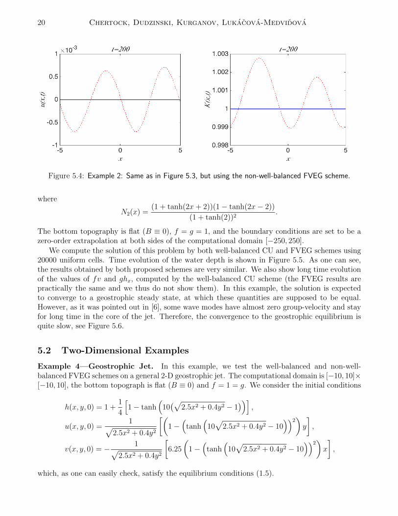
Example 2—Geostrophic Steady State with a Periodic Bottom. We now take the samecomputational domain [−5, 5], but use periodic boundary conditions. The bottom topography isgiven by

B(x) =f

gsin(π

5x), f = 1 = g,

and the flow is initially at the geostrophic equilibrium, namely:

K(x) ≡ 1, v(x) =π

5cos(π

5x), u(x) ≡ 0.

The periodic boundary conditions are implemented in the following way. We use two ghostcells on both sides of the computational domain for the variables u, v, h and B, which are periodic.However, the potential V as well as the equilibrium variable K are not necessarily periodic andthus should be treated in a different way: We only assign their values at the ghost cell C0 bysetting V0 := ∆x

2(v−1 + v0) and then computing K0 from (1.6).

As in Example 1, the well-balanced CU scheme as well as the well-balanced FVEG schemepreserves this steady state within the machine accuracy. At the same time, their versions that usea non-well-balanced piecewise linear reconstruction lead to appearance of the artificial waves. Thiscan be seen in Figures 5.3 and 5.4, where we plot the equilibrium variables u and K, computedusing a uniform grid with 200 cells at time T = 200 by the well-balanced CU scheme togetherwith the same quantities computed by non-well-balanced CU (Figure 5.3) and FVEG (Figure 5.4)schemes. For both schemes, the amplitudes of the artificial waves are proportional to the size ofthe local truncation errors.

Figure 5.3: Example 2: Equilibrium variables (u ≡ 0, K ≡ 1) computed by the well-balanced (solidline) and non-well-balanced (solid line with dots) CU schemes.

Example 3—Rossby Adjustment in an Open Domain. In this example taken from [6] (seealso [8, 36]) we numerically solve the 1-D system (1.9), (1.10) subject to the following initial data:

h(x, 0) ≡ 1, u(x, 0) ≡ 0, v(x, 0) = 2N2(x),


Figure 5.4: Example 2: Same as in Figure 5.3, but using the non-well-balanced FVEG scheme.

where

N2(x) =(1 + tanh(2x+ 2))(1− tanh(2x− 2))

(1 + tanh(2))2.

The bottom topography is flat (B ≡ 0), f = g = 1, and the boundary conditions are set to be azero-order extrapolation at both sides of the computational domain [−250, 250].

We compute the solution of this problem by both well-balanced CU and FVEG schemes using20000 uniform cells. Time evolution of the water depth is shown in Figure 5.5. As one can see,the results obtained by both proposed schemes are very similar. We also show long time evolutionof the values of fv and ghx, computed by the well-balanced CU scheme (the FVEG results arepractically the same and we thus do not show them). In this example, the solution is expectedto converge to a geostrophic steady state, at which these quantities are supposed to be equal.However, as it was pointed out in [6], some wave modes have almost zero group-velocity and stayfor long time in the core of the jet. Therefore, the convergence to the geostrophic equilibrium isquite slow, see Figure 5.6.

5.2 Two-Dimensional Examples

Example 4—Geostrophic Jet. In this example, we test the well-balanced and non-well-balanced FVEG schemes on a general 2-D geostrophic jet. The computational domain is [−10, 10]×[−10, 10], the bottom topograph is flat (B ≡ 0) and f = 1 = g. We consider the initial conditions

h(x, y, 0) = 1 +1

4

[1− tanh

(10(√

2.5x2 + 0.4y2 − 1))]

,

u(x, y, 0) =1√

2.5x2 + 0.4y2

[(1−

(tanh

(10√

2.5x2 + 0.4y2 − 10))2

)y

],

v(x, y, 0) = − 1√2.5x2 + 0.4y2

[6.25

(1−

(tanh

(10√

2.5x2 + 0.4y2 − 10))2

)x

],

which, as one can easily check, satisfy the equilibrium conditions (1.5).


Figure 5.5: Example 3: Time evolution of h computed by the well-balanced CU (◦’s) and FVEG (×’s)schemes.

We would like to point out that the well-balanced reconstruction presented in §2 as well as thewell-balanced evolution operators (4.11), (4.14) are constructed in such a way that they preservetwo particular jets in the rotational frame, (1.7) and (1.8), only. Nevertheless, the well-balancedfinite-volume schemes developed in this paper also approximate general 2-D geostrophic jets in a


Figure 5.6: Example 3: Long time evolution of fv (dashed-dotted line) and ghx (solid line) computedby the well-balanced CU scheme.

more accurate and stable way than their non-well-balanced counterparts. To demonstrate this,we present, in Figure 5.7, a long time evolution of Kx and Ly, computed using a coarse uniformmesh with 50× 50 cells.

Example 5—Stationary Vortex. In the last numerical experiment, which is a slight modifi-cation of the test problem proposed in [2], we consider a stationary vortex in the square domain[−1, 1]× [−1, 1] with the boundary conditions set to be a zero-order extrapolation in both x- andy-directions. We take the flat bottom topography (B ≡ 0), f = 1/ε and g = 1/ε2 with ε = 0.05,


Figure 5.7: Example 4: Long time evolution of the L2-norm of Kx and Ly computed by the second-order well-balanced (solid line) and non-well-balanced (dashed line) FVEG schemes. To plot thesecurves, we have used a cubic smoothing spline representation.

which correspond to a low Mach number regime (see [2]), and the following initial conditions:

h(r, 0) = 1 + ε2

5

2(1 + 5ε2)r2, r <

1

5

1

10(1 + 5ε2) + 2r − 1

2− 5

2r2 + ε2(4 ln(5r) +

7

2− 20r +

25

2r2),

1

5≤ r <

2

5,

1

5(1− 10ε+ 4ε2 ln 2), r ≥ 2

5,

u(x, y, 0) = −εyΥ(r), v(x, y, 0) = εxΥ(r), Υ(r) :=

5, r <

1

52

r− 5,

1

5≤ r <

2

5,

0, r ≥ 2

5,

where r :=√x2 + y2.

We compute the numerical solutions by both the well-balanced and non-well-balanced schemes.In the following, we present the results obtained by the CU schemes using a 200× 200 grid. Thetime evolution of the errors, ||h(x, y, 0)−h(x, y, t)||L2 , presented in Figure 5.8 clearly demonstratesthat our well-balanced method outperforms the non-well-balanced one. Indeed, as time evolvesthe error of the non-well-balanced CU scheme increases considerably in comparison with the well-balanced CU scheme. This fact is also demonstrated in Figure 5.9, where the correspondingnumerical solutions at time T = 10 are presented. One can clearly see the structural deficiency ofthe non-well-balanced solution that does not preserve the circular symmetry of the vortex, whichis dissipated much more when the non-well-balanced CU scheme is used. We note that thoughthe considered stationary vortex is not a discrete steady state of the well-balanced CU scheme, itpreserves the initial vortex structure in a much better way.


Figure 5.8: Example 5: Comparison of time evolution of the L2-errors obtained by the well-balancedand non-well-balanced CU schemes.

Conclusions

In this paper, we have studied preservation of nontrivial equilibrium states, the so-called jets in therotational frame (1.7), (1.8) that appear in the shallow water equations with the Coriolis forces.This is a model typically used in the oceanographic applications. We would like to point outthat in comparison with the lake at rest equilibria (h + B ≡ Const, u ≡ v ≡ 0), the geostrophicequilibria (1.7), (1.8) are much harder to preserve since some of the equilibrium variables are nowglobally defined potentials.

In §2, we have derived a new second-order well-balanced reconstruction and proved that ityields well-balanced schemes. In order to illustrate a generality of our approach, we have shownhow the new well-balanced reconstructions can be incorporated into the framework of the central-upwind and finite-volume evolution Galerkin schemes. It should also be pointed out that for thelatter scheme the evolution operator has been carefully derived to evolve the equilibrium variables.We have proven that the proposed schemes exactly preserve jets in the rotational frame steadystates (1.7), (1.8). The importance of this property has been illustrated in a number of numericalexamples, where small perturbations of the steady states have been considered. Furthermore, wehave shown that although our well-balanced finite-volume methods do not preserve general 2-Dgeostrophic jets exactly, they still approximate them more accurately than the corresponding non-well-balanced finite-volume schemes. We believe that the proposed approach can be extended tomultilayer shallow water equations, for which we have already developed the second-order central-upwind [10, 28] and finite-volume evolution Galerkin [13] schemes.

Acknowledgment. The work of A. Chertock was supported in part by the NSF Grants DMS-1216974 and DMS-1521051 and the ONR Grant N00014-12-1-0832. The work of A. Kurganovwas supported in part by the NSF Grants DMS-1216957 and DMS-1521009 and the ONR GrantN00014-12-1-0833. M. Lukacova was supported by the German Science Foundation (DFG) GrantsLU 1470/2-3 and SFB TRR 165 “Waves to Weather”. We would like to thank Doron Levy(University of Maryland) and Leonid Yelash (University of Mainz) for fruitful discussions on


Figure 5.9: Example 5: Stationary vortex computed at T = 10 by the well-balanced (left) and non-well-balanced (right) CU schemes. Top view (top row) and the 1-D slice along y = 0 (bottom row).

the topic.

A Derivation of FVEG Evolution Operators

In this section, we derive new well-balanced evolution operators Econstτ (4.11) and Ebilin

τ (4.14),used in (4.2), (4.3) and (4.4) with τ = ∆t/2. Here, we only show how to evolve the values of thepotentials K and L, since the evolution equations for the velocities u and v have been presentedin [36].

The solution is going to be evolved from time tn to time tn + τ and we are going to use the


following notations, which are similar to the notations that were used in §4:

P := (x, y, tn + τ), Q0(t) :=(x− u∗(tn + τ − t), y − v∗(tn + τ − t), t

),

Q(t) :=(x− [u∗ − c∗ cos θ](tn + τ − t), y − [v∗ − c∗ sin θ](tn + τ − t), t), t ∈ [tn, tn + τ),

where, as before, θ ∈ (0, 2π], and u∗, v∗ and c∗ are the local velocities and speed of gravity wavesat the point (x, y, tn). Note that P is the vertex of the bicharacteristic cone, Q0(t) are the pointsalong the cone axis, Q(t) are the points on the mantle of the cone, and, in particular, Q(tn) arethe points at the perimeter of the sonic circle at time tn.

In order to obtain an expression for the evolution operators for K and L, we first write the exactintegral equation for water depth h, which can be derived using the theory of bicharacteristics,see [36, (A5)]:

h(P ) =1

2π

2π∫0

[h(Q(tn))− c∗

g

(u(Q(tn)) cos θ − v(Q(tn)) sin θ

)]dθ

− 1

2π

tn+τ∫tn

[1

tn + τ − t

2π∫0

c∗

g

(u(Q(t)) cos θ + v(Q(t)) sin θ

)dθ

]dt

+c∗

2π

tn+τ∫tn

2π∫0

[Bx(Q(t)) cos θ +By(Q(t)) sin θ

]dθdt

− c∗

2π

tn+τ∫tn

2π∫0

[Vx(Q(t)) cos θ − Uy(Q(t)) sin θ

]dθdt.

(A.1)

We now rewrite the last integral on the RHS of (A.1) as

tn+τ∫tn

2π∫0

[Vx(Q(t)) cos θ − Uy(Q(t)) sin θ

]dθdt

=

tn+τ∫tn

2π∫0

[Vx(Q(t)) cos θ + Vy(Q(t)) sin θ

]dθdt−

tn+τ∫tn

2π∫0

[Vy(Q(t)) cos θ + Uy(Q(t)) sin θ

]dθdt

(A.2)Applying the rectangle rule for time integration and the Taylor expansion about Q0(tn), we canshow that the last integral in (A.2) is of order O(τ 2):

tn+τ∫tn

2π∫0

[Vy(Q(t)) cos θ + Uy(Q(t)) sin θ

]dθdt

=

2π∫0

[Vy(Q(tn)) cos θ + Uy(Q(tn)) sin θ

]dθ +O(τ 2)

= Vy(Q0(tn))

2π∫0

cos θ dθ + Uy(Q0(tn))

2π∫0

sin θ dθ +O(τ 2) = O(τ 2).


To evaluate the first integral on the RHS of (A.2), we introduce polar-type coordinates along themantle of the bicharacteristic cone

ξ = x+ r(

cos θ − u∗

c∗

), η = y + r

(sin θ − v∗

c∗

),

where r = c∗(tn + τ − t) is the circle radius at time level t ∈ [tn, tn + τ ]. Thus, we have

dV

dr(r, θ) = Vx(ξ, η) cos θ + Vy(ξ, η) sin θ − 1

c∗

(u∗Vx(ξ, η) + v∗Vy(ξ, η)− Vt(ξ, η)

),

and hence we obtaintn+τ∫tn

2π∫0

[Vx(Q(t)) cos θ + Vy(Q(t)) sin θ

]dθdt

= − 1

c∗

0∫c∗τ

2π∫0

dV (r, θ)

drdθdr +

1

c∗

tn+τ∫tn

2π∫0

[u∗Vx(Q(t)) + v∗Vy(Q(t)) + Vt(Q(t))

]dθdt

=1

c∗

c∗τ∫0

d

dr

( 2π∫0

V (r, θ) dθ

)dr +

1

c∗

tn+τ∫tn

2π∫0


]dθdt

=1

c∗

( 2π∫0

V (Q(tn)) dθ − 2πV (P )

)+

1

c∗

tn+τ∫tn

2π∫0


]dθdt.

(A.3)

Similarly, the third integral on the RHS of (A.1) is equal to

tn+τ∫tn

2π∫0

[Bx(Q(t)) cos θ +By(Q(t)) sin θ

]dθdt

=1

c∗

( 2π∫0

B(Q(tn)) dθ − 2πB(P )

)+

1

c∗

tn+τ∫tn

2π∫0

[u∗Bx(Q(t)) + v∗By(Q(t))

]dθdt,

(A.4)

since Bt ≡ 0.Combining (A.1), (A.3) and (A.4), we obtain the following approximation of the exact integral

equations for K = g(h+B − V ):

K(P ) =1

2π

2π∫0

[K(Q(tn))− c∗

(u(Q(tn)) cos θ + v(Q(tn)) sin θ

)]dθ

− 1

2π

tn+τ∫tn

[1

tn + τ − t

2π∫0

c∗(u(Q(t)) cos θ + v(Q(t)) sin θ

)dθ

]dt

+g

2π

tn+τ∫tn

2π∫0

[u∗Bx(Q(t)) + v∗By(Q(t))

]dθdt

− g

2π

tn+τ∫tn

2π∫0


]dθdt.

(A.5)


This formula provides the evolution equation for the equilibrium variable K. Our next goal isto approximate time integrals in (A.5) in a suitable way, so that we obtain explicit approximateevolution operators for Econst

τ (4.11) and Ebilinτ (4.14). This will be realized in a standard way

following [35] and a superscript I will be used for piecewise constant approximations, while asuperscript II will be used for piecewise linear ones.

For the piecewise constant approximations, the spatial derivatives are zero and thus the cor-responding integral terms in (A.5) vanish. Therefore, using the fact that

tn+τ∫tn

2π∫0

V It (Q(t)) dθdt = 2π

[V I(P )− V I(Q0(tn))

]+O(τ 2) (A.6)

and approximating the mantle integral of uI(Q(t)) cos θ+vI(Q(t)) sin θ according to [35], we obtain

KI(P ) ≈ 1

2π

2π∫0

[KI(Q(tn))− c∗

(uI(Q(tn))sgn(cos θ) + vI(Q(tn))sgn(sin θ)

)]dθ

+ g[V I(Q0(tn))− V I(P )

],

which leads to (4.11).

For the piecewise linear approximations, the spatial derivatives do not vanish and we approxi-mate the integrals in the corresponding terms in (A.5) by the rectangle rule to obtain

tn+τ∫tn

2π∫0

[u∗V II

x (Q(t)) + v∗V IIy (Q(t))

]dθdt = τ

2π∫0

[u∗V II

x (Q(tn)) + v∗V IIy (Q(tn))

]dθ +O(τ 2),

which, together with a similar approximation of the bottom topography terms, leads to (4.14).Indeed, applying (A.6) and the standard approximation for the mantle integral of uII(Q(t)) cos θ+vII(Q(t)) sin θ as in [35], we finally obtain

KII(P ) = KII(Q0(tn)) +1

4

2π∫0

(KII(Q(tn))−KII(Q0(tn))

)dθ

− c∗

π

2π∫0

(uII(Q(tn)) cos θ + vII(Q(tn)) sin θ

)dθ

+τ

2π

2π∫0

[u∗(KIIx (Q(tn))− ghII

x (Q(tn)))

+ v∗(KIIy (Q(tn))− ghII

y (Q(tn)))]dθ

+ g[V II(Q0(tn))− V II(P )

].

Notice that the derivation of the approximate evolution operators for LI(P ) and LII(P ) isanalogous.


References

[1] E. Audusse, F. Bouchut, M.-O. Bristeau, R. Klein, and B. Perthame, A fast andstable well-balanced scheme with hydrostatic reconstruction for shallow water flows, SIAM J.Sci. Comput., 25 (2004), pp. 2050–2065.

[2] E. Audusse, R. Klein, D. D. Nguyen, and S. Vater, Preservation of the DiscreteGeostrophic Equilibrium in Shallow Water Flows, in Finite Volumes for Complex ApplicationsVI Problems & Perspectives, vol. 4 of Springer Proceedings in Mathematics, Springer BerlinHeidelberg, 2011, pp. 59–67.

[3] E. Audusse, R. Klein, and A. Owinoh, Conservative discretization of Coriolis force ina finite volume framework, J. Comput. Phys., 228 (2009), pp. 2934–2950.

[4] A. Bollermann, G. Chen, A. Kurganov, and S. Noelle, A well-balanced reconstruc-tion of wet/dry fronts for the shallow water equations, J. Sci. Comput., 56 (2013), pp. 267–290.

[5] N. Botta, R. Klein, S. Langenberg, and S. Lutzenkirchen, Well balanced finitevolume methods for nearly hydrostatic flows, J. Comput. Phys., 196 (2004), pp. 539–565.

[6] F. Bouchut, J. Le Sommer, and V. Zeitlin, Frontal geostrophic adjustment and nonlin-ear wave phenomena in one-dimensional rotating shallow water. II. High-resolution numericalsimulations, J. Fluid Mech., 514 (2004), pp. 35–63.

[7] S. Bryson, Y. Epshteyn, A. Kurganov, and G. Petrova, Well-balanced positivitypreserving central-upwind scheme on triangular grids for the Saint-Venant system, M2ANMath. Model. Numer. Anal., 45 (2011), pp. 423–446.

[8] M. J. Castro, J. A. Lopez, and C. Pares, Finite volume simulation of the geostrophicadjustment in a rotating shallow-water system, SIAM J. Sci. Comput., 31 (2008), pp. 444–477.

[9] A. Chertock, S. Cui, A. Kurganov, and T. Wu, Well-balanced positivity preservingcentral-upwind scheme for the shallow water system with friction terms, Internat. J. Numer.Meth. Fluids, 78 (2015), pp. 355–383.

[10] A. Chertock, A. Kurganov, Z. Qu, and T. Wu, Three-layer approximation of two-layer shallow water equations, Math. Model. Anal., 18 (2013), pp. 675–693.

[11] P. J. Dellar and R. Salmon, Shallow water equations with a complete Coriolis force andtopography, Phys. Fluids, 17 (2005), p. 106601.

[12] M. Dudzinski, Well-balanced bicharacteristic-based finite volume schemes for multilayershallow water systems, PhD thesis, Technische Universitat Hamburg-Harburg, 2014.

[13] M. Dudzinski and M. Lukacova-Medvidova, Well-balanced bicharacteristic-basedscheme for multilayer shallow water flows including wet/dry fronts, J. Comput. Phys., 235(2013), pp. 82–113.

[14] T. Gallouet, J.-M. Herard, and N. Seguin, Some approximate Godunov schemes tocompute shallow-water equations with topography, Comput. & Fluids, 32 (2003), pp. 479–513.


[15] E. Godlewski and P.-A. Raviart, Numerical approximation of hyperbolic systems ofconservation laws, vol. 118 of Applied Mathematical Sciences, Springer-Verlag, New York,1996.

[16] S. Gottlieb, D. Ketcheson, and C.-W. Shu, Strong stability preserving Runge-Kuttaand multistep time discretizations, World Scientific Publishing Co. Pte. Ltd., Hackensack, NJ,2011.

[17] S. Gottlieb, C.-W. Shu, and E. Tadmor, Strong stability-preserving high-order timediscretization methods, SIAM Rev., 43 (2001), pp. 89–112.

[18] A. Hundertmark, M. Lukacova-Medvidova, and F. Prill, Large time step finitevolume evolution Galerkin methods, J. Sci. Comp., 48 (2011), pp. 227–240.

[19] S. Jin, A steady-state capturing method for hyperbolic systems with geometrical source terms,M2AN Math. Model. Numer. Anal., 35 (2001), pp. 631–645.

[20] R. Klein, Scale-dependent models for atmospheric flows, Annu. Rev. Fluid Mech., 42 (2010),pp. 249–274.

[21] D. Kroner, Numerical schemes for conservation laws, Wiley-Teubner Series Advances inNumerical Mathematics, John Wiley & Sons Ltd., Chichester, 1997.

[22] A. C. Kuo and L. M. Polvani, Wave-vortex interaction in rotating shallow water. I. Onespace dimension, J. Fluid Mech., 394 (1999), pp. 1–27.

[23] A. C. Kuo and L. M. Polvani, Nonlinear geostrophic adjustment, cyclone/anticycloneasymmetry, and potential vorticity rearrangement, Phys. Fluids, 12 (2000), pp. 1087–1100.

[24] A. Kurganov and D. Levy, Central-upwind schemes for the Saint-Venant system, M2ANMath. Model. Numer. Anal., 36 (2002), pp. 397–425.

[25] A. Kurganov and C.-T. Lin, On the reduction of numerical dissipation in central-upwindschemes, Commun. Comput. Phys., 2 (2007), pp. 141–163.

[26] A. Kurganov, S. Noelle, and G. Petrova, Semi-discrete central-upwind scheme forhyperbolic conservation laws and Hamilton-Jacobi equations, SIAM J. Sci. Comput., 23 (2001),pp. 707–740.

[27] A. Kurganov and G. Petrova, A second-order well-balanced positivity preserving central-upwind scheme for the Saint-Venant system, Commun. Math. Sci., 5 (2007), pp. 133–160.

[28] A. Kurganov and G. Petrova, Central-upwind schemes for two-layer shallow waterequations, SIAM J. Sci. Comput., 31 (2009), pp. 1742–1773.

[29] A. Kurganov and E. Tadmor, New high resolution central schemes for nonlinear conser-vation laws and convection-diffusion equations, J. Comput. Phys., 160 (2000), pp. 241–282.

[30] A. Kurganov and E. Tadmor, Solution of two-dimensional Riemann problems for gasdynamics without Riemann problem solvers, Numer. Methods Partial Differential Equations,18 (2002), pp. 584–608.


[31] R.J. LeVeque, Balancing source terms and flux gradients in high-resolution Godunov meth-ods: the quasi-steady wave-propagation algorithm, J. Comput. Phys., 146 (1998), pp. 346–365.

[32] R.J. LeVeque, Finite volume methods for hyperbolic problems, Cambridge Texts in AppliedMathematics, Cambridge University Press, Cambridge, 2002.

[33] K.-A. Lie and S. Noelle, On the artificial compression method for second-order nonoscil-latory central difference schemes for systems of conservation laws, SIAM J. Sci. Comput., 24(2003), pp. 1157–1174.

[34] M. Lukacova-Medvidova, K. W. Morton, and G. Warnecke, Evolution Galerkinmethods for hyperbolic systems in two space dimensions, MathComp., 69 (2000), pp. 1355–1384.

[35] M. Lukacova-Medvidova, K. W. Morton, and G. Warnecke, Finite volume evolu-tion Galerkin methods for hyperbolic systems, SIAM J. Sci. Comp., 26(1) (2004), pp. 1–30.

[36] M. Lukacova-Medvidova, S. Noelle, and M. Kraft, Well-balanced finite volumeevolution Galerkin methods for the shallow water equations, J. Comp. Phys., 221 (2007),pp. 122–147.

[37] A. Majda, Introduction to PDEs and waves for the atmosphere and ocean, vol. 9 of CourantLecture Notes in Mathematics, New York University, Courant Institute of MathematicalSciences, New York; American Mathematical Society, Providence, RI, 2003.

[38] H. Nessyahu and E. Tadmor, Nonoscillatory central differencing for hyperbolic conserva-tion laws, J. Comput. Phys., 87 (1990), pp. 408–463.

[39] S. Noelle, N. Pankratz, G. Puppo, and J.R. Natvig, Well-balanced finite volumeschemes of arbitrary order of accuracy for shallow water flows, J. Comput. Phys., 213 (2006),pp. 474–499.

[40] S. Noelle, Y. Xing, and C.-W. Shu, High-order well-balanced finite volume WENOschemes for shallow water equation with moving water, J. Comput. Phys., 226 (2007), pp. 29–58.

[41] J. Pedlosky, Geophysical Fluid Dynamics, Springer-Verlag, New York, 2nd ed., 1987.

[42] G. Russo, Central schemes for conservation laws with application to shallow water equations,in Trends and Applications of Mathematics to Mechanics, Springer Milan, 2005, pp. 225–246.

[43] A. L. Stewart and P. J. Dellar, Multilayer shallow water equations with completeCoriolis force. Part 1. Derivation on a non-traditional beta-plane, J. Fluid Mech., 651 (2010),pp. 387–413.

[44] A. L. Stewart and P. J. Dellar, Two-layer shallow water equations with completeCoriolis force and topography, in Progress in industrial mathematics at ECMI 2008, vol. 15of Math. Ind., Springer, Heidelberg, 2010, pp. 1033–1038.

[45] P. K. Sweby, High resolution schemes using flux limiters for hyperbolic conservation laws,SIAM J. Numer. Anal., 21 (1984), pp. 995–1011.


[46] E.F. Toro, Riemann solvers and numerical methods for fluid dynamics: A practical intro-duction, Springer-Verlag, Berlin, Heidelberg, third ed., 2009.

[47] G. K. Vallis, Atmospheric and Oceanic Fluid Dynamics: Fundamentals and Large-ScaleCirculation, Cambridge University Press, 2006.

[48] B. van Leer, Towards the ultimate conservative difference scheme. V. A second-order sequelto Godunov’s method, J. Comput. Phys., 32 (1979), pp. 101–136.

[49] Y. Xing and C.-W. Shu, A new approach of high order well-balanced finite volume WENOschemes and discontinuous Galerkin methods for a class of hyperbolic systems with sourceterms, Commun. Comput. Phys., 1 (2006), pp. 100–134.

well-balanced schemes for the shallow water equations with ... · in many situations steady-state...

Documents