Welcome to Yagi-World

L. B. Cebik, W4RNL1434 High Mesa Drive

Knoxville, TN 37938-4443e-mail: cebik@cebik.com

A typical QRP operator loves simple antennas. However, temptation comes to us all at one oranother time. The lure of DX, competition, or simply the desire to have reliable communications with afamily member or dear friend is often enough to bring thoughts of directional beams. Among directionalantennas, the Yagi-Uda (or Yagi, for short) parasitic array is now the gold standard. That is, the Yagibrings in more gold to antenna makers than any other type of amateur antenna.

Along with the gold, commercially made Yagis carry with them a number of mysteries, calledspecifications. Like all commercial products, let the buyer beware. If you have some remodeling workdone to your home, unless you know the differences between good and bad materials and practices, youmay not be able to tell whether the builders did a good or bad job until the work fails. Likewise, unlessyou know something about Yagis, you may not be able to tell the difference between a good and a baddesign until it is too late to correct an error in your buying judgment.

So my premise is simple. Let's survey some of the key elements in Yagi performance to obtain abackground against which we can make intelligent judgments about the Yagi that we might buy.Welcome to the world of Yagis.

The Weighty Basics

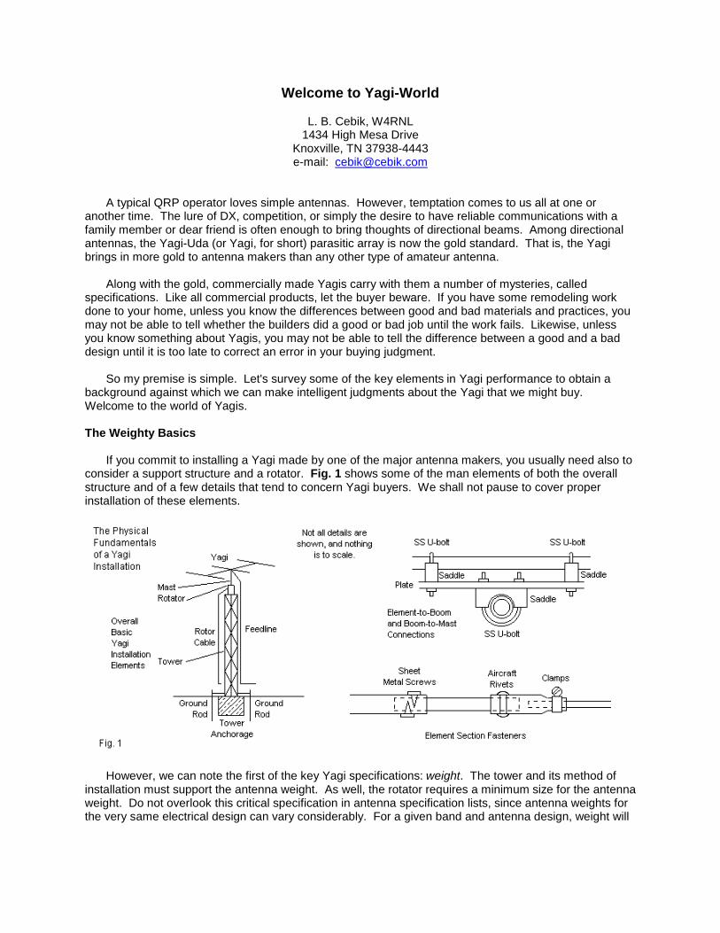
If you commit to installing a Yagi made by one of the major antenna makers, you usually need also toconsider a support structure and a rotator. Fig. 1 shows some of the man elements of both the overallstructure and of a few details that tend to concern Yagi buyers. We shall not pause to cover properinstallation of these elements.

However, we can note the first of the key Yagi specifications: weight. The tower and its method ofinstallation must support the antenna weight. As well, the rotator requires a minimum size for the antennaweight. Do not overlook this critical specification in antenna specification lists, since antenna weights forthe very same electrical design can vary considerably. For a given band and antenna design, weight will

vary according to the materials used. We can conveniently divide the world into three antennaconstruction materials.

1. The American Oak: The most common tubular material used in Yagi construction is 6063-T832 aircraftaluminum tubing. In the U.S., the material is readily available for home brew Yagis from a variety ofsources. American tubing typically comes in eighth-inch steps, with 0.56" thick walls for perfect nestingfrom one size to the next. The material is strong and returns to shape after wind forces try to bend it. Infact, making an intentional bend requires special procedures to prevent cracking at the bend.

2. The American Willow: Some antenna makers use thinner wall tubing without loss of strength in thewind. One way to tell if the tubing is thinner than the de facto oak standard is the use of slight diameterreductions at every junction. These antennas can cut the weight of a given design by up to about 1/3rd

and include the use of lighter boom material. Willow-based antennas will show more deflection in thewind, but may be as strong as oak-based designs--if we construct the elements properly.

3. The European Ironwood: Today, we have access to many well-designed Yagis made in Europe.Typically, Europeans do not have access to the same sizes of aircraft aluminum that are common in theU.S. Metric aluminum (or aluminium, in the Commonwealth) tends to step in metric sizes with a basic 2-mm wall thickness--about 0.079". For a given element design, the elements will be heavier--up to about 2times heavier than an equivalent U.S. design. The added element weight calls for a heavier boom with athicker wall, and the hardware size increases at every step of the assembly. Hence, with few exceptions,European Yagis tend to weigh considerably more than their U.S. counterparts.

The result is a simple question for the total Yagi installation: how much weight are you willing tohandle when sizing all of the components to match? Unlike current medical concerns about the U.S.population, lightness in Yagis is not always a virtue, and heaviness is not always a vice. However, asystem that mismatches its support, rotating, and antenna components is always a disaster waiting tohappen.

Gravity is not the only force acting on a Yagi. Every antenna is subject to wind loading. We expectwire antennas to break periodically under forces created by the wind (including the deflection ofsupporting structures). So we do not bother with wind-load specification. However, we do expect Yagisto last forever, given the size of our investment in them. Therefore, every Yagi carries with it a maximumwind-survival rating and a wind-area. The wind area relates mostly to matching the antenna to therotator, which has a brake or hold-in-position mechanism that works only until the winds and the antennaarea exceed ratings. Then the mechanism lets the antenna rotate, either by design or by theunintentional destruction of an internal part.

The overall wind-survival rating rests on the combination of materials and element construction. Theuse of tapered element diameters in Yagi construction is no accident. Except at 10 meters and upward,uniform diameter tubing in amateur Yagis would simply snap in high winds. A steady high wind mayactually succeed in bending antenna elements. Either case is fatal to antenna performance. By thejudicious selection of element segment lengths--aided by computer computations these days--antennamakers can create elements that will survive high winds. Very often, the second section from the elementcenter may extend all the way through the first section to double the wall thickness for extra strength.Yagis for 40 through 20 meters often use this technique to improve the wind-survival rating.

Typically, amateur Yagis have wind-survival ratings from 80 to 120 mph, depending on price and thecall to makers for heavy duty versions of their antennas. The U.S. government has readily availablemaps that list the highest winds expected in every county in the country. Be certain that any Yagi thatyou buy or build will have a wind survival rating that exceeds the value for your county. Alternatively (oradditionally), consider countermeasures against the wind, such as a tower that you can lower whenexpecting bad weather.

There is one final wind-loading factor: the mast that extends from the rotator to the boom. Even if it isquite short, never use pipe material for the mast. Use a rated tube material. Pipe material is soft andintended to bend under external pressure. Pipe is stiff. It deflects the wind.

When you survey your choices for a given Yagi design, do not neglect the hardware and method ofassembly. All hardware should be stainless steel. Galvanized hardware may be suitable for outdoordecking, but not for antennas. Likewise plated steel is forbidden. Besides the problem of rusting, moststeel hardware will create bi-metallic electrolysis with the aluminum elements and results in fairly rapiddeterioration of the junction. Stainless steel is immune to the effect.

Element and boom saddles should be solid for American oak or willow elements to reduce thechances of element crushing during assembly. Many European designs use muffler-clamp saddles--usually without the teeth on their edges--a practice that is generally satisfactory with the thicker-wallelement tubing.

Element section fasteners generally come in 3 varieties and breed some of the longest-standingcontroversies in antenna work. Where two sections of an element overlap, we can fasten them with sheetmetal screws, clamps, or aircraft (not hobbyist) rivets. One maker uses rivets exclusively, and his willow-based designs have shown no unusual problems. Most commonly, standard steps of aluminum handlestainless steel sheet metal screws quite well, although some antenna users report loosening with time. Afew makers still use clamps at element section junctions. Be sure to coat the overlapping junctions andfastener contact areas with conductive anti-seizing compound to allow disassembly of the antenna after afew years of service in the weather.

I shall pass over all mechanical and electrical safety measures, as well as means of attenuatingcommon-mode currents, since our goal is the beam itself. Finally, be certain that you schedule andperform periodical preventive maintenance inspections and tests on the same regular (6-month) basisthat you use for your trusty wire antennas.

The Maze of Electrical Specifications for Monoband Yagis

To obtain a grasp of basic Yagi specifications, I shall start from scratch and assume no knowledge ofthe rudimentary terms associated with antenna radiation patterns. Those with modeling or other antennadesign and analysis experience may slumber momentarily, but a review has never proven fatal to anyone.Fig. 2 presents the free-space radiation pattern of a typical long-boom 3-element Yagi. The pattern istechnically not an azimuth pattern, because in free space we have no way to distinguish up and downfrom side-to-side. E-plane patterns are generally in the plane of the elements. (For 3-D quads, they arein the plane of the element portions contributing most to the radiation.)

Conventionally, we represent the radiation pattern on a polar plot, although rectangular graphing isalso possible. The plot style most commonly used is called the ARRL log scale, because the power gainlevels (recorded here in decibels or dB) use a logarithmic scale from the outer ring down to the center.The center point value is so low that it is nearly infinitesimal. We might have arranged the power levelvalues on a linear scale, but that would force us to select for each pattern a minimum level for the centerpoint--and what we select for the minimum can change the pattern appearance significantly. So we shallstay with the ARRL log scale. (In QST, you will see different main rings for values below the outer ring,so always be sure to look at the scale used from outer ring to center point.) Furthermore, the pattern isnormalized so that the maximum gain of the antenna in any sampled direction just reaches the outer ring.Therefore, every other ring in the pattern shows how much weaker (in dB) the pattern is relative to themaximum gain.

A Yagi pattern has two main parts: the forward and the rearward pattern components. Thecomponents consist of one or more lobes (regions that culminate in a maximum strength point), andintervening nulls. For the subject antenna, there is only 1 forward lobe, also called the main forward lobe.The rearward components show why we add the word "main" to lobe terms. The rearward portion of thepattern has 3 lobes. With Yagis, we conventionally call the rearward lobe in line with the main forward

lobe the main rearward lobe. (Note that the main rearward lobe need not be the strongest lobe to therear, although the main forward lobe is almost always the lobe showing the highest gain level.) Lobesthat go off in other directions become sidelobes. Forward sidelobes are also possible, but simply do notappear on Yagis this short.

The angular lines in the main forward lobe indicate the directions at which the gain drops by 3 dBrelative to the maximum forward gain of the antenna. The other name for these lines is the half-powerpoints. The number of decrees between these lines defines by convention the antenna beamwidth. If wecount radiating dotted lines on this EZNEC plot, we shall discover that the beamwidth for the subjectantenna is a bit over 60°. Finally, note the deep nulls on each side of the pattern, 90° away from themaximum-gain heading. You will only see nulls this deep on free-space patterns. So if an antennamaker displays patterns having nulls that go all the way to the center-point, you know that he generatedthem with a free-space model.

One of the most basic antenna specifications that you will find in maker literature is the front-to-backratio. Precisely here we must pause, not only to grasp the terminology, but as well to learn a bit offlexibility in our thinking. First, not everyone uses the basic term in the same way. So we shall find somerefinements in the terminology. Second, not everyone who uses the refined terminology uses it in thesame way. Our goal is not to say who is right and who is wrong. Instead, our goal is to learn the rightquestions to ask so that we can find out what a maker means by his use of "front-to-back ratio." Table 1and Fig. 3 will be our guides, but only for part of the journey. Both the table and the graphic presentinformation on the rearward performance of 3 sample antennas. Numbers and pictures do not alwaysdetermine how people use words. Therefore, we shall proceed along one fork in the front-to-back road,and then we shall backtrack and proceed down the other path. The lesson that we shall learn is not totake at face value everything that appears on a road sign.

Our first step will be to present some initial definitions (with modifications to come). These definitionswill coincide with the labels in Table 1. The 180° front-to-back ratio is the main lobe forward gain (or themaximum antenna gain) minus the gain of the lobe (however big or small) that is 180° away from theheading of the maximum forward gain. This value of front-to-back ratio is most commonly used in generalantenna literature and is the one shown in most NEC antenna software. If the main forward lobe is splitor does not align with the graph heading, the 180° front-to-back ratio is 180° away from the direction ofmaximum pattern strength. Hence, the value may not be for a direction directly to the rear of the antennastructure. Since a Yagi is usually symmetrical, the maximum gain will normally be directly forward, andthe 180° front-to-back ratio will indicate the relative strength to the direct rear. Note that if we use anormalized scale, we can read the front-to-back ratio directly from the plot--between 25 and 30 dB relativeto the maximum gain of the antenna in the leftmost pattern.

In Fig. 3, the leftmost pattern comes from Fig. 2. The strongest rearward lobe is 180° from the mainlobe. However, the center pattern shows a 180-degree gain of very tiny proportions. Hence, the 180°front-to-back ratio is very large (over 40 dB compared to a "mere" 27 dB for the leftmost pattern). Yet, wefind rearward lobes that have considerable strength. The line through one of those lobes indicates thedirection of maximum strength. It is only about 22 dB weaker than the maximum gain. Some sources callthis the worst-case front-to-back ratio, and its value is the maximum forward gain minus the highest valueof gain in either rearward quadrant. For this antenna, the 180° front-to-back ratio does not give a truepicture of the QRM levels from the rear, so some folks prefer to use this figure as a better indicator. Theworst-case front-to-back ratio provides the most conservative value for rearward suppression of QRM.The rightmost graphic in Fig. 3 shows that the 180° and the worst-case front-to-back values do notrequire separate lobes, even thought the values differ. (We may debate elsewhere whether the 8-element Yagi main rearward radiation is a single main lobe or a junction of 3 overlapping lobes.) Whenwe find the two ratios related to the same rearward lobe, we usually do not find much difference in theirvalue.

We are not done with front-to-back ratios. Each sketch in Fig. 3 contains an arc going from 90° onone side of the line of maximum gain around the rear to the other point that is 90° from the maximum gainline. Suppose that we add up all of the gain values at the headings that pass through the arc. Next taketheir average value. Subtract the average gain value to the rear from the maximum forward gain and youarrive at what some call the front-to-rear ratio. Others call this the averaged front-to-back ratio. Table 1

performs this task at 5° intervals, which is sufficient for this sampling. If you compare the front-to-rearratio with the other front-to-back ratios, you can see why an antenna maker might use it. The value ishigher than all of the other values (with the exception of the 180° front-to-back ratio for the 3-elementshort-boom Yagi). The rationale behind using the front-to-rear ratio is that it provides an averaged totalpicture of the rearward QRM suppression. At least one maker uses this technique for rearwardspecifications.

The usages listed here, although fairly old, are not universal. For example, ARRL's antenna literature(including the influential Antenna Book) uses "front-to-rear ratio" to mean what we have here called the"worst-case front-to-back ratio." You may, of course, select your personal favorite set of terms, but that isunimportant when you are in the market for a Yagi. The key question is this one: what term does eachmaker use for rearward evaluation, and what does he mean by that term? Until you have that knowledgein hand, you cannot compare beams sold by separate makers.

If all Yagi makers used free-space patterns as the basis for their specification lists, we might have aneasy time sorting them out. However, some makers use a ground reference. Therefore, we need tomaster not only free-space patterns, but patterns taken over ground as well. This process begins byunderstanding more fully the difference between the two sets of plots. Here we can turn to Fig. 4.

On the left, we find a 3-element Yagi (our long-boom sample) and the E-plane and H-plane patternsassociate with the free-space environment. As noted earlier, the E-plane pattern aligns with the planeformed by the 3 elements. The H-plane pattern is at right angles to the E-plane pattern, when bothpatterns use the same heading for maximum gain. Note that the patterns meet at the maximum gainpoint and again at the point that is 180° from the maximum gain heading.

If we place the antenna over ground, both patterns undergo critical shifts in what they show. Wechange the pattern names to elevation and azimuth, since we now have a ground reference and potentialcompass headings. The sample on the right places the antenna 1 λ above average ground. Normally,the elevation pattern aligns with the maximum gain heading--but it need not do so. Besides showingmultiple elevation lobes, the Yagi's maximum gain now occurs 14° above the horizon, the take-off angle.The take-off angle will vary with the antenna height (and, as we shall soon see, with the antenna forwardgain). For most purposes, we then obtain an azimuth pattern at the take-off angle, as shown by the dotthat indicates a meeting of the two patterns. (Once more, we can take the azimuth pattern at anyelevation angle, assuming that we have a reason to do so.) Note that every point on the azimuth patternoutline is elevated 14°, not just the maximum forward gain heading. When we obtain a front-to-back ratio,it implies an azimuth comparison only, so that the sampled rear lobes or lobes are also at the same

elevation angle. The comparison may or may not show the point where a rear lobe is strongest orweakest, since that point may occur at a different elevation angle.

Let's add one more final note about pattern conventions. The patterns that we have shown emergefrom the exact center of the antenna geometry, not from the driver or any other particular element. Thereason that we use this convention lies in the different sizes of the components of each sketch. A far-fieldradiation pattern extends outward an indefinitely large distance. In fact, the distance is so large that bycomparison, the antenna is infinitesimally small. Even a visible dot would be technically too large toindicate the antenna size. If we shrink the antenna to its proper scale for the pattern shown, then it willwithdraw uniformly down to an invisible dot at the very center of the pattern. Hence, when we draw thepattern and the antenna so that both are visible, we expand in the reverse direction, and the antennacenter becomes the origin of the radiation plot.

We are now ready to tackle the basic concepts of reporting the maximum forward gain of a Yagi. Asindicated in Table 2, we have a number of choices available, and the shaded entries indicate the onesmost commonly used. For reference, I have added a dipole to the 3-element long-boom Yagi that is ourfundamental sample.

The most common 21st century power gain reference is dBi, meaning the power gain of the antennain the favored direction as measured in dB over an isotropic source. An isotropic source is one thatradiates equally at all elevation and azimuth angles, forming a perfect sphere, if we could model thepattern. Although some folks have developed antennas that radiate in an isotropic manner, the isotropicradiator is a useful tool in calculating power gain, since all power gain numbers use a single standard ofcomparison. PowerdB = 10 log10(Power1/PowerRef). If the reference is isotropic, then the power gain termis dBi. (If a maker specifies simply dB, then the reference is anybody's guess in the absence of anexplanatory footnote.) In the table, a standard dipole made from aluminum and as thick as the Yagielements has a free-space gain of 2.13 dBi, while the Yagi has a free-space gain of 8.11 dBi. This resultgives the Yagi a 5.98-dB gain over an equivalent dipole in free space.

The alternative standard for power gain measurement is dBd, meaning the power gain of the antennain the favored direction as measured in dB over a theoretic dipole. A theoretic dipole is composed oflossless wire that is infinitesimally thin. It has by calculations from basic antenna theory a gain of 2.15 dBover an isotropic source. Hence, the difference between dBi and dBd is always exactly 2.15 dB. In free-space, the Yagi has a gain of 5.96 dBd, but the thick aluminum dipole has a gain of -0.02 dBd. The gainof the Yagi over the thick dipole in free space remains 5.98 dB. Although the use of dBi seems lessconfusing, the dBd measure is still popular with some antenna makers, especially in Europe. In the U.S.,makers who model or measure their beam performance over ground still favor dBd.

Let's move our antennas to exactly 1 λ above average ground and re-model them. The Yagi shows amaximum gain of 13.34 dBi and 11.19 dBd. The lower number might sound more conservative, but ithides a deceit, since it seems to imply that the gain of the Yagi is 11.19 dB over a dipole. However, a realdipole at the same height has a gain of 7.63 dBi and 5.48 dBd. The thick dipole has a gain of 5.48 dBover a dipole. We shall be stuck in a conundrum unless we clearly specify that the real dipole has gain

over the theoretical foundation of dBd measurements. In fact, over ground, whether we use dBi or dBd,the Yagi has a gain of 5.71 dB over a real dipole at the same height over the same ground quality.

In free space, the Yagi showed 5.98-dB gain over the real dipole, but 1 λ over average ground, thegain advantage dropped to 5.71 dB. Although the difference is too small to be operationally detected, westill must wonder what happened to the 0.28 dB. The answer lies in the basic antenna losses and theground losses that result in the reflection amount that we add to the direct gain. As we shall soon see,the higher the initial gain and the larger the number of elements in our Yagi, the lower grows theincrement of additional gain that we accrue by placing the antenna over a fixed ground at a fixed height.

Some makers give their maximum gain values in free-space terms, using either dBi or dBd. Othermanufacturers model or measure their antenna forward gain values at some height above ground. Theymay or may not specify the ground quality, and they may give the height in terms of feet or other physicalmeasure or in terms of wavelengths above ground. If the frame of reference is not clear in a specificationsheet, then you have some questions to ask before you start making comparative performancejudgments. As well, our brief notes only provide a modicum of translation guidance. For example, if onemaker gives specifications for 70' for all antennas, that height is 1 λ only on 20 meters. It is 2 λ on 10meters. If another maker uses a 1-λ height for all specifications, then you can easily compare 20-meterYagis, but not 10-meter Yagis.

Further confusion enters the playing ground because too few amateurs contemplating their first Yagiknow what to expect from the antenna. To provide a partial remedy for this situation, Table 3 presentssome free-space modeling figure for Yagis ranging from 2 to 8 elements. The table lists the forward gainin dBi, the 180° front-to-back value, the horizontal (or E-plane) beamwidth, and the rough feedpointimpedance.

Yagi designs come in many forms, so understanding the remaining table data requires a few notes.First, we may design Yagis with a fixed number of elements over a range of boomlengths. Even the 2-element driver-reflector Yagis have one boom length for maximum gain and front-to-back ratio, andanother that is more suitable for a wide-band match with a direct 50-Ω cable connection to the driving

element. The 3 element Yagi shows 3 variations in ascending boomlengths as measured in wavelengths.For longer Yagis, I have selected a relatively short-boom and a relatively long-boom model. At 6elements and up, the short-boom models use design principles to provide stable wide-band performanceand a direct 50-Ω coax connection (with the usual common-mode attenuator, of course). The finalcolumn indicates whether a manufactured beam of a given type would employ a matching networkbetween the driver and the coax (M) or simply make a direct connection (D). Matching networks areneither good nor bad in themselves. They do provide a few more components to go bad in the weather,not to mention additional connections to corrode. But good manufacturing techniques can result in long-term reliable assemblies.

The tabulated monoband Yagis intended for a matching network show impedance values very closeto resonance. In such cases, one might use a quarter-wavelength matching section to arrive at 50 Ohms.By making the element shorter, we do not disturb the performance of Yagis that have at least 3 elements,but we do set up a capacitive reactance in the driver that is suitable for both a beta (hairpin) or a gammamatch. I have seen no evidence (amid much manufacturer palaver) that any one system is intrinsicallybetter than another. Remember that the matching network affects only the SWR performance of theantenna and not its gain or other basic performance properties.

The data show increasing gain values (within limits from one model to the next). As gain increases,the horizontal beamwidth decreases. Fig. 5 provides a gallery of free-space E-plane patterns (almost thesame as azimuth patterns above 1 λ antenna height). The collection shows the progression of forwardpatterns shapes as the gain grows higher. Note especially the emergence of forward sidelobes:minuscule in 5L10L but ever more definite in the L-type patterns as the number of elements goes from 5to 8. Of course, the boomlength also increases in this same range.

The S-series of Yagis shows lesser sidelobe development. The weaker forward sidelobes do notresult so much from the shorter boomlength, but from the special arrangement of elements, the samearrangement that allows for direct 50-Ω feed connections with no intervening matching network. Thetabular data also show that we pay a small gain price for the privilege of forward lobe shaping andperformance stabilization.

Table 4 moves the same set of typical Yagi designs from free space to a position 1 λ above averageground. To the table, we add a new column to record the take-off angle. The angle drops by 1° as wemove from 4 to 5 elements--or more precisely, from a half-wavelength boom to one that is about 5/8-λlong. Gain tends to be more a function of boom length than of the exact element count, although toobtain a beam with adequate feedpoint impedance and operating bandwidth, the variation in elementnumbers for a given gain level and boomlength is minimal. We have already seen that tailoring theelements on a given boomlength for special performance properties may also exact a small gain penalty.

Re-examine the patterns for the 3-element long-boom Yagi in any of the early figures. I calledattention to the deep insets or nulls 90° either side of the main lobe bearing. Fig. 6 providessupplementary elevation and azimuth patterns for the same beam at different heights above ground: 0.5,1.0, and 1.5 λ. The elevation patterns will be virtually identical for all of the Yagi designs in the tables.We acquire a new elevation lobe for each half wavelength of height. The lobes do not suddenly appear ateach height. Rather, they emerge as an increase in gain straight up and as we move the antenna a bithigher, they tilt over in the forward direction. A corresponding tilt also occurs in the rearward direction,but the rear elevation lobes tend to be too small for us to bother noticing.

The forward lobes of the azimuth patterns appear to be virtually the same. As we raise the height ofthe antenna, the gain slowly increases as the take-off angle decreases. However, the most notable gainincreases occur from near ground level to about 1-λ high, as the ground exerts ever-weaker effects uponperformance. The most dramatic affects of ground proximity involve the rear lobes and the side nulls ofthe free-space pattern. The closer the antenna is to ground, the shallower are the side nulls. At a heightof 0.5 λ, the nulls do not appear. Instead we have only a squaring of the pattern on the way to the rearsidelobes. As we continue to raise the antenna, the side nulls appear and grow stronger. However, evenat a height of 1.5 λ, the nulls are considerably weaker than in the free-space pattern. These phenomena,

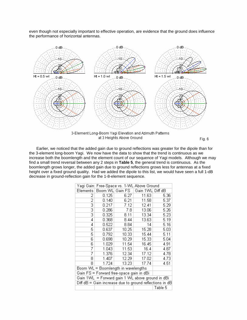
even though not especially important to effective operation, are evidence that the ground does influencethe performance of horizontal antennas.

Earlier, we noticed that the added gain due to ground reflections was greater for the dipole than forthe 3-element long-boom Yagi. We now have the data to show that the trend is continuous as weincrease both the boomlength and the element count of our sequence of Yagi models. Although we mayfind a small trend reversal between any 2 steps in Table 5, the general trend is continuous. As theboomlength grows longer, the added gain due to ground reflections grows less for antennas at a fixedheight over a fixed ground quality. Had we added the dipole to this list, we would have seen a full 1-dBdecrease in ground-reflection gain for the 1-8-element sequence.

The sequence of beams has something in common. They all are designed at the middle of an HFham band (in this case, 28.5 MHz). The gain values are not necessarily peak values, since at the designfrequency, each beam is a compromise aiming at the best combination of gain, front-to-back ratio, andSWR bandwidth. The gain values give you a ballpark number to use in reading antenna makerspecification sheets. Once you translate them into the terms that the maker uses, you can detect valuesthat are grossly under- or over-stated. Normally you will see higher values for antennas with the samenumber of elements and comparable boomlengths. Makers like to site the optimistic peak gain within theoperating passband rather than the mid-band or average gain value.

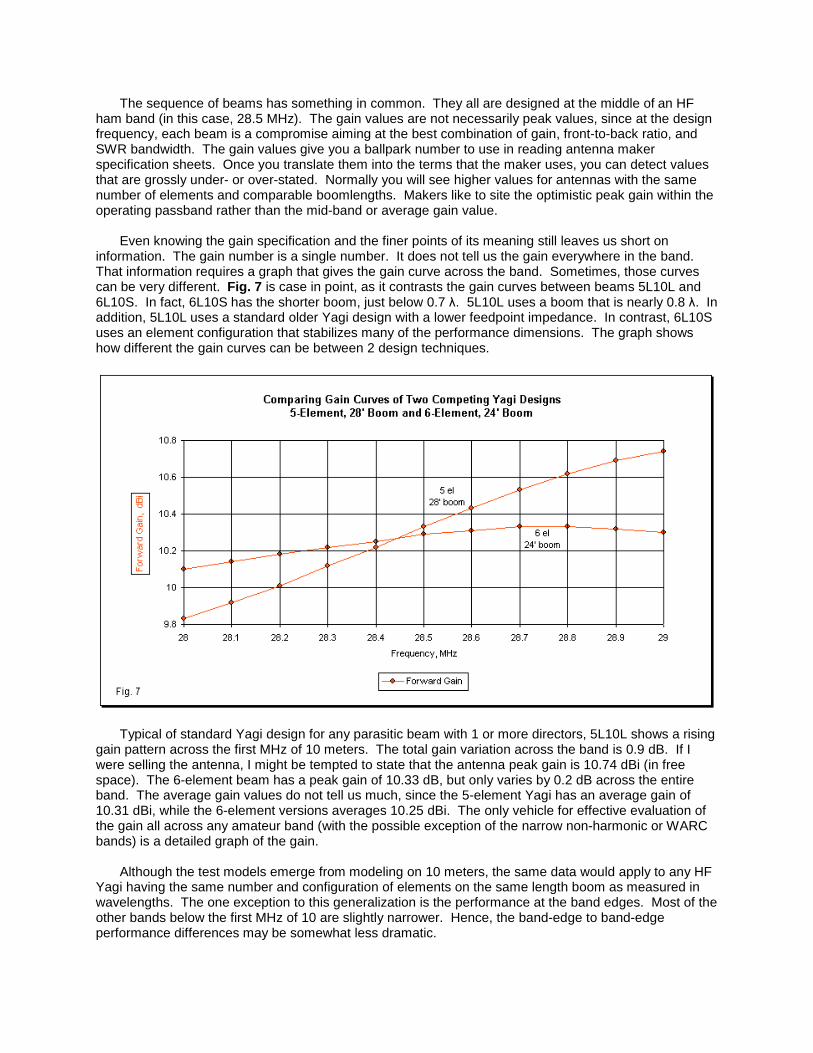
Even knowing the gain specification and the finer points of its meaning still leaves us short oninformation. The gain number is a single number. It does not tell us the gain everywhere in the band.That information requires a graph that gives the gain curve across the band. Sometimes, those curvescan be very different. Fig. 7 is case in point, as it contrasts the gain curves between beams 5L10L and6L10S. In fact, 6L10S has the shorter boom, just below 0.7 λ. 5L10L uses a boom that is nearly 0.8 λ. Inaddition, 5L10L uses a standard older Yagi design with a lower feedpoint impedance. In contrast, 6L10Suses an element configuration that stabilizes many of the performance dimensions. The graph showshow different the gain curves can be between 2 design techniques.

Typical of standard Yagi design for any parasitic beam with 1 or more directors, 5L10L shows a risinggain pattern across the first MHz of 10 meters. The total gain variation across the band is 0.9 dB. If Iwere selling the antenna, I might be tempted to state that the antenna peak gain is 10.74 dBi (in freespace). The 6-element beam has a peak gain of 10.33 dB, but only varies by 0.2 dB across the entireband. The average gain values do not tell us much, since the 5-element Yagi has an average gain of10.31 dBi, while the 6-element versions averages 10.25 dBi. The only vehicle for effective evaluation ofthe gain all across any amateur band (with the possible exception of the narrow non-harmonic or WARCbands) is a detailed graph of the gain.

Although the test models emerge from modeling on 10 meters, the same data would apply to any HFYagi having the same number and configuration of elements on the same length boom as measured inwavelengths. The one exception to this generalization is the performance at the band edges. Most of theother bands below the first MHz of 10 are slightly narrower. Hence, the band-edge to band-edgeperformance differences may be somewhat less dramatic.

We can find differences in front-to-back performance that also depend upon graphs that cover theentire operating passband for a Yagi. Let's compare the 180° front-to-back ratio for the same 2 antennas.Fig. 8 gives us the data.

We can make the 5-element Yagi stand out by citing the peak front-to-back ratio: about 39 dB.However, the 180° front-to-back ratio varies across the band from the peak value down to 14 dB. Incontrast, the 6-element beam shows only a 9-dB variation in front-to-back ratio, varying from a low of 21dB to a high of over 30 dB. In this comparison, the average front-to-back ratio values would tell us verylittle, since they are within about 0.8 dB of each other.

We can easily jump to the conclusion that the graph shows the 6-element Yagi to be superior. Thatjudgment has no meaning, since it does not tell us in what respect the beam is better. The 6-elementbeam is superior in the smoothness of its operating curve across the band. However, if we need thefront-to-back ratio at the low end of the band, then the 5-element beam wins the comparison. Part ofcomparing beams rests on deciding what you want from a Yagi and where you want it. Nevertheless, wecould not even begin to make the comparison unless we have the detailed data graph. Given the currentprices of monoband beams, demanding performance curves for the band in question is not merelyreasonable. If the maker wants your money, he will send the curves or show you where they areavailable on the web. If he will not go this far to support your purchase, then I might have strongquestions about his reliability in standing behind the product.

If you can obtain the antenna manual in advance, you likely can model each Yagi that is a candidate.Modeling will not only confirm the maker's claims, but can also put a pattern face on the raw numbers.Fig. 9 presents band-edge and mid-band free-space E-plane patterns for the two Yagis that we havebeen using for our sample gain and front-to-back curves. In many ways, at least through the middle ofthe band, there are no decisive radiation pattern traits that would lead us to select one over the otherbeam. The high-end patterns might tip the scale--if using the upper portion of the band is sufficientlyimportant. (On 20 and 15 meters, the high-end performance would determine how well the design worksin the most active SSB portion of those bands.) The 5-element beam shows that it is near the limits ofperformance at the listed boomlength. The front-to-back ratio has fallen off, resulting in a sizable mainrear lobe. In addition, we can notice the emergence of forward sidelobes. These sidelobes are notserous, unless we allow for manufacturing variations. In contrast, the 6-element high-end pattern showsthe same cleanliness that characterizes the patterns for frequencies lower in the band.

Even if these patterns do not lead us to a decision about which hypothetical beam to purchase, theyare still worthy of study. The more we know about the antennas that we buy or build, the morereasonable will be our expectations of them.

So far, we have said nothing about the impedance performance of the antennas that we havesurveyed as typical representatives in the HF range. For this specification, most makers are all too happyto shows 50-Ohm SWR curves. At worst, they assure us that the SWR is under 2:1 at the limits of thepassband and often that the design-frequency SWR is 1:1. What makers rarely tell us is how theyobtained the numbers. If a beam requires an impedance matching network, we know that it must be inplace. However, the specification sheets rarely tell us whether the SWR applies at the antenna terminalsor after some intervening length of coax. If we can infer the use of coax--as we can for at least onemaker who specifies Yagis above 70' over ground--we usually do not know what coax he used to makemeasurements. All of these considerations make a difference in the claims that we can make about Yagiperformance.

To demonstrate the difference, I provided the 3-element long-boom Yagi with a quarter-wavelengthmatching section so that the impedance at 28.5 MHz was 50.00 - j0.007 Ω. Then I ran a frequencysweep and recorded the impedances and 50-Ω SWR from 28.0 to 29.0 MHz in 0.1-MHz increments. Thenext step involved using the program TLW that comes with The ARRL Antenna Book. For the impedanceat each frequency, I connected a 75' length of coaxial cable and read out both the impedance and theSWR. I repeated the exercise for 3 different 50-Ω cables: low-loss LMR400, common RG-213, andequally common RG-8X, the so-called low-loss thinner cable. However, the 3 cables show increasinglosses from LMR400 through RG-213 down to RG8X. Each cable has a different velocity factor, so theelectrical length of each cable in the tests differed slightly. However, the test focused on using aphysically constant length of cable.

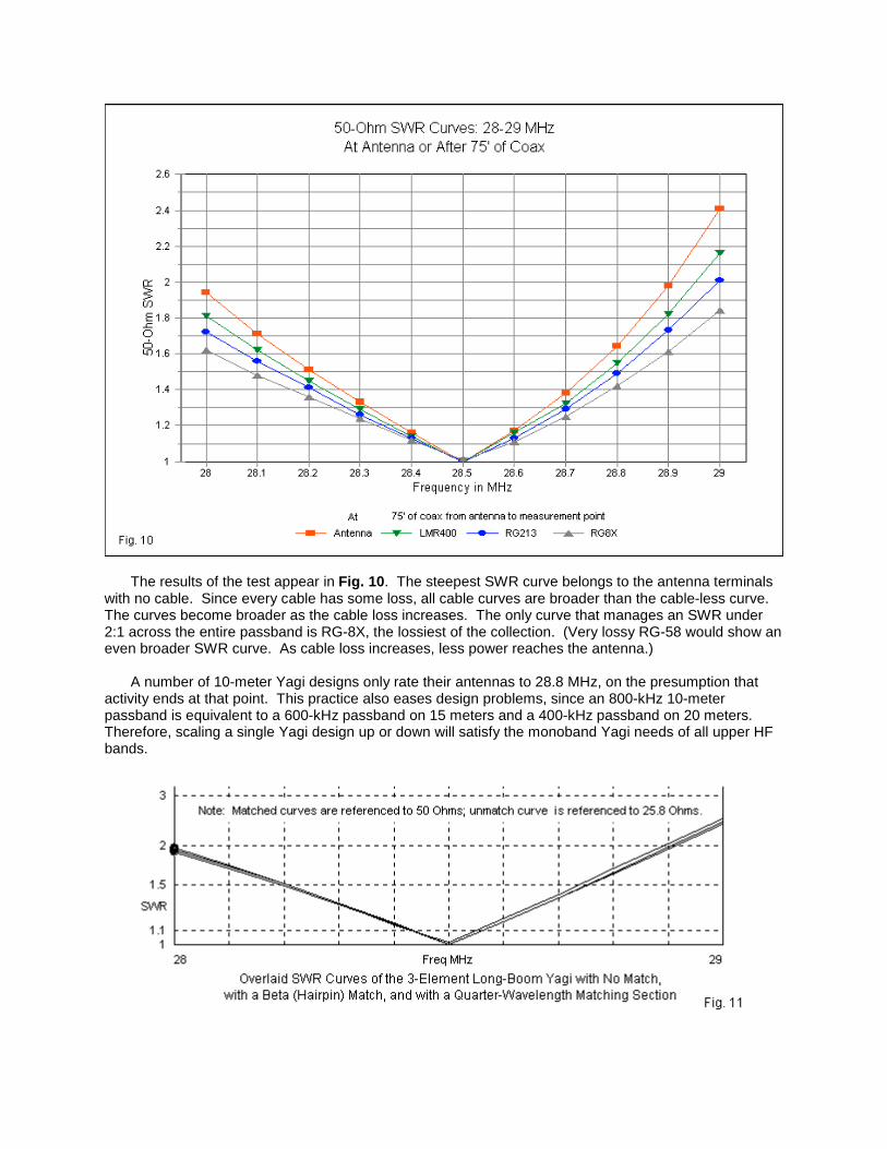
The results of the test appear in Fig. 10. The steepest SWR curve belongs to the antenna terminalswith no cable. Since every cable has some loss, all cable curves are broader than the cable-less curve.The curves become broader as the cable loss increases. The only curve that manages an SWR under2:1 across the entire passband is RG-8X, the lossiest of the collection. (Very lossy RG-58 would show aneven broader SWR curve. As cable loss increases, less power reaches the antenna.)

A number of 10-meter Yagi designs only rate their antennas to 28.8 MHz, on the presumption thatactivity ends at that point. This practice also eases design problems, since an 800-kHz 10-meterpassband is equivalent to a 600-kHz passband on 15 meters and a 400-kHz passband on 20 meters.Therefore, scaling a single Yagi design up or down will satisfy the monoband Yagi needs of all upper HFbands.

Note that the SWR curve is quite sharp and rises more steeply above the design frequency thanbelow it. The curve properties are quite normal for virtually any Yagi of standard design that has at leastone director. The rate of change of SWR above and below the design frequency is normal regardless ofthe type of matching section used. Fig. 11 shows overlaid SWR curves for the sampled 3-element Yagiwithout a match and with 2 different types of matching sections: a quarter-wavelength line and a beta orhairpin match. Some curves shown by antenna makers are so smooth that one has to wonder how muchloss the measuring system has.

Not all SWR curves are alike. Fig. 12 samples some variations. At the top, the 3-element short-boom Yagi has a typical small-Yagi curve, very much like the one for the long-boom 3-element Yagi. Thesecond curve--for the 5-element long-boom Yagi--shows favoritism for the lower end of the passband.Indeed, some commercial Yagi designs will ask the user to select the desired portion of the band andadjust the assembly measurements to produce the SWR curve that most favors the selection. As Yagisgrow longer, we find that designers use broadband techniques, since they normally do not change thetotal boom length by much. Hence, the 7-element long-boom Yagi provides a shallow SWR curve,although the reference impedance tells us that it still needs a matching network for a 50-Ω cable.

The last curve in the set is typical of the Yagis receiving special design considerations for a directconnection to 50-Ω cable. The design produces no frequency at which the impedance is exactly 50 Ω,but it remains very close to 50 Ω across the entire band. Hence, the SWR never quite reaches 1.4:1anywhere within the first MHz of 10 meters. The curve serves as a counterweight to placing too muchemphasis on commercial claims that a Yagi's SWR is 1:1 at the design frequency. Often, there are goodreasons for not having a perfect 1:1 SWR at the design frequency if we can hold the SWR very lowacross a wide band of frequencies.

We have reached the end of our basic introduction to the world of commercial monoband Yagis. Wehave covered enough information to allow you to understand and even translate maker specifications intoa uniform set of information so that you can compare antennas before buying. The data on typical short-and long-boom Yagis designs, both in free space and 1 λ above ground provides a set of ballpark valuesso that you can evaluate gain claims. You may extrapolate probable values for boomlengths and elementcounts that do not appear on the list. If you cannot translate a maker's claims and terms into values thatmake sense relative to the data tables, you should send inquiries to the maker. His patience andhelpfulness during the decision process is often a good indicator of probable after-sale support to you.

As an exercise, I am providing the following sample specifications drawn from the literature of variousantenna makers. Since this is only a sample, I have not listed explicit maker names. Furthermore,specifications change over time, so the list will soon be dated. In some cases, the meaning of aspecification is clear as given. In other cases, other portions of the literature will make it clear. However,sometimes, nothing may clarify a listed specification except an explicit question to the maker. Everyantenna maker wants to present his products in the most favorable light. Your job is to change the rose-colored advertising glow into the bright white of clarity and full information. If you need motivation, scanthe price lists for monoband Yagis.

A Random Sample of Mono-Band Yagi Specifications

Maker H HBand 10 20No. Elements 3 3Boom Length (ft) 8 (0.23 λ) 16.5 (0.24 λ)Weight (lb) 15 32Gain (free space) 7.5 dBi 7.15 dBiF-B FR: 24 dB max FR: 23 dB maxSWR 1.25:1 at resonance <1.5:1 at resonance

Maker C C CBand 10 10 20No. Elements 3 4 4Boom Length (ft) 10 (0.29 λ) 16 (0.46 λ) 32.7 (0.47 λ)Weight (lb) 11 18 55Gain 8.0 dBd (unspecified) 10.0 dBd (unspecified) 10.0 dBd (unspecified)F-B 30 dB (unspecified) 30 dB (unspecified) 30 dB (unspecified)SWR 1.2:1 1.2:1 <1.5:1

Maker M M MBand 10 20 20No. Elements 4 4 5Boom Length (ft) 24 (0.69 λ) 34.7 (0.5 λ) 44 (0.63 λ)Weight (lb) 20 36 105Gain (free space) 8 dBd 7.34 dBd 8.1-8.5 dBdF-B FR: 22 dB typical FR: 23 dB typical FR: 24 dB typicalSWR 1.25:1 typical 1:1 at resonance 1:1 at resonance

Maker F F FBand 20 20 20No. Elements 5 6 7Boom Length (ft) 36 (0.52 λ) 44 (0.63 λ) 58 (0.84 λ)Gain (at 74') 7.3 dBd net 7.8 dBd net 8.4 dBd netF-B FR: 23 dB average FR: 23 dB average FR: 23 dB averageSWR <1.6:1 <1.4:1 <1.5:1

Tri-Band Yagi Compromises

Just when I though our work might be complete, someone asked, "What about tri-band Yagis?" Theidea of obtaining Yagi performance for three different bands on one boom has great appeal. Anyone witha computer and antenna modeling software might develop a quite reasonable monoband Yagi. Butsqueezing full performance out of interlaced elements for 3 bands involves far more than 3 times thelabor of a monoband Yagi.

Let's see what might be involved in tri-band design. Suppose that we want to have a 3-element Yagi.If we select a monoband design, then a given design on 20 meters will have a boom that is twice as longas the same design on 10 meters. The earliest tri-band Yagis simply chose a compromise spacing andthrew traps into the elements so that they would show a resonant point on 10, 15, and 20 meters. In the1970s and 1980s, every Yagi builder assumed his beam reached full theoretical performance, and so thegain claims for these 3-element compromise arrays were unbelievably optimistic. With the advent ofcomputer modeling software, designers went back to the drawing boards.

Today's tri-banders tend to look nothing like those of past decades. Very few use traps, althoughsome older designs are still available. Nevertheless, tri-band designs involve compromises. Forexample, modern trapless designs tend to add 10-meter elements to fill a boom and therefore obtainbetter than 3-element performance on that band. However, with a common driver or set of driverelements, one of the 10-meter directors tends to want to be just where the 20-meter director lies. A 20-meter director will tend to dominate the 10-meter pattern and change the 10-meter passband to reducethe operating range at the high end of the band. One corrective is for the designer to add an extradirector so that 2 10-meter directors bracket the 20-meter director to neutralize the dominance factor. Sowe cannot determine performance simply by counting elements on each band (although we always dojust that as a matter of course).

As well, we now see a variety of different ways to provide a common feedpoint for all 3 bands. Asingle driving element with traps appears in some designs. One maker uses a log-cell driver section, aset of driving elements connected very much like the elements in a log periodic dipole array. We also findseparate driving elements for each band, but there are at least 2 arrangements. One system makes adirect connection between drivers, using a short length of parallel transmission line. An alternativemethod uses open-sleeve coupling so that only the 20-meter driver has a connection to the feedline. Bycareful selection of the length and close spacing of each "slaved" driver for the other bands, highefficiency coupling occurs, although it is difficult to obtain full band coverage from a slaved driver. All ofthe systems work, but the trapped driver is perhaps the least efficient. However, traps do reduce the totalnumber of elements needed by a tri-band for a given boomlength, since some elements may do double ortriple duty.

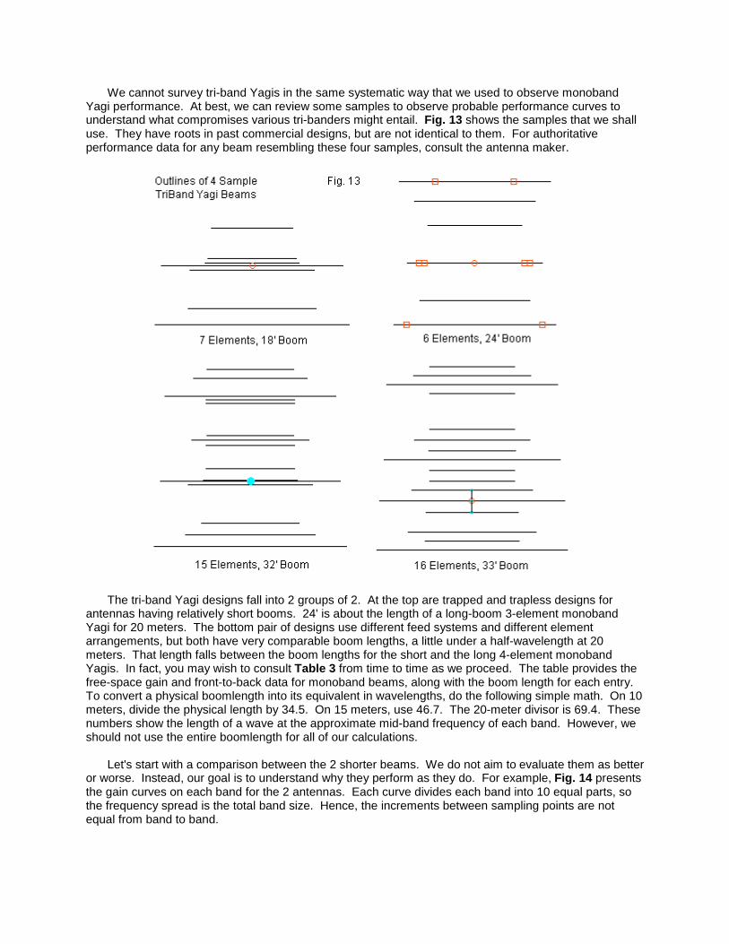
We cannot survey tri-band Yagis in the same systematic way that we used to observe monobandYagi performance. At best, we can review some samples to observe probable performance curves tounderstand what compromises various tri-banders might entail. Fig. 13 shows the samples that we shalluse. They have roots in past commercial designs, but are not identical to them. For authoritativeperformance data for any beam resembling these four samples, consult the antenna maker.

The tri-band Yagi designs fall into 2 groups of 2. At the top are trapped and trapless designs forantennas having relatively short booms. 24' is about the length of a long-boom 3-element monobandYagi for 20 meters. The bottom pair of designs use different feed systems and different elementarrangements, but both have very comparable boom lengths, a little under a half-wavelength at 20meters. That length falls between the boom lengths for the short and the long 4-element monobandYagis. In fact, you may wish to consult Table 3 from time to time as we proceed. The table provides thefree-space gain and front-to-back data for monoband beams, along with the boom length for each entry.To convert a physical boomlength into its equivalent in wavelengths, do the following simple math. On 10meters, divide the physical length by 34.5. On 15 meters, use 46.7. The 20-meter divisor is 69.4. Thesenumbers show the length of a wave at the approximate mid-band frequency of each band. However, weshould not use the entire boomlength for all of our calculations.

Let's start with a comparison between the 2 shorter beams. We do not aim to evaluate them as betteror worse. Instead, our goal is to understand why they perform as they do. For example, Fig. 14 presentsthe gain curves on each band for the 2 antennas. Each curve divides each band into 10 equal parts, sothe frequency spread is the total band size. Hence, the increments between sampling points are notequal from band to band.

The first notable feature for the shortest 7-element, 18' antenna is that the curves for 20 and 15 arevery similar, with slow downward slopes, but the curve for 10 meters has a very steep upward slope. Ifyou examine the outline in Fig. 13, you can identify the 2 active 20-meter elements and the 2 active 15-meter elements. Each pair forms a driver-reflector 2-element Yagi, and the gain curves for those bands fittypical monoband performance for wide 2-element spacing. However, the 10-meter elements are alldirectors, and so the curve is upward with frequency increases. For each band, the effective boom lengthfor the individual bands is only about half of the total boomlength.

The lower part of Fig. 14 shows gain curves for the 24' trapped model. The 4 elements on 10 metersshow a steep upward gain slope. The three 15-meter elements have long-boom spacing, but there is atrap on each side of the driver. So the performance is more akin to a short-boom monoband Yagi.Where traps take their greatest toll is on 20 meters, where we find 2 traps on each side of the driver andsingle traps on each side of the parasitic elements.

Fig. 15 shows the 180° front-to-back curves for the 2 antennas. The 7-element antenna showscomparable 20- and 15-meter values that are on a par with 2-element monoband Yagis. The curve for 10meters shows higher values, but still under the 20-dB value that is typical for a well-designed monobandshort-boom 3-element Yagi. Since we have 2 major elements on 20, 2 on 15, and 3 on 10 meters, thebeam obtains about all that we can expect from its design.

The trapped 24' Yagi shows generally superior front-to-back ratios on 10 and 15 meters, although 15meters has an average value under 20 dB. The sharp peak in the 10-meter curve is movable with slightadjustments to the element lengths inside the traps. On 20 meters, the multitude of traps at work reducesthe ratio for the 3 active elements down to 2-element Yagi levels. In general, the compromise elementspacing of most tri-band beams usually results in reduced front-to-back performance relative tomonoband Yagis with the same boomlength between the limiting active elements.

Fig. 16 supplies modeled 50-Ohm SWR curves for the 2 sample antennas. The upper curves for the7-element, 18' design shows one recurring challenge for open-sleeve coupling in tri-banders: reducedoperating bandwidth. The challenge shows up on 15-meter, where the beam covers only about 80% ofthe band at 2:1 SWR or better.

The lower set of curves for the trapped models shows 2 facts. First, the 20-meter curve is notaccurate, since the actual beam has a matching section not used in the model. The matched curve wouldreach very close to 1:1 at mid-band and simple be lower overall. Traps shorten the overall elementlengths for the lower bands, creating challenges for full band coverage. The 10-meter curve shows asharpness that reflects the sharp front-to-back curve. One property common to many trapped designs isthe need to favor either the lower end or the upper end of the wide ham bands.

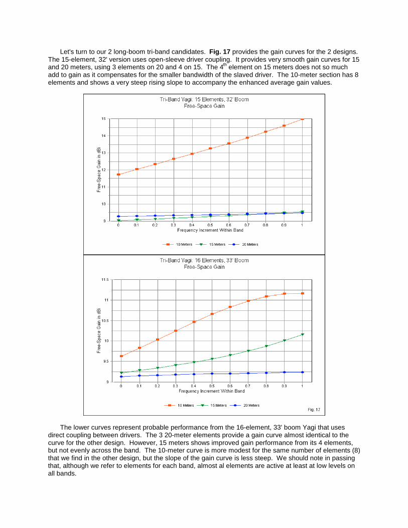
Let's turn to our 2 long-boom tri-band candidates. Fig. 17 provides the gain curves for the 2 designs.The 15-element, 32' version uses open-sleeve driver coupling. It provides very smooth gain curves for 15and 20 meters, using 3 elements on 20 and 4 on 15. The 4th element on 15 meters does not so muchadd to gain as it compensates for the smaller bandwidth of the slaved driver. The 10-meter section has 8elements and shows a very steep rising slope to accompany the enhanced average gain values.

The lower curves represent probable performance from the 16-element, 33' boom Yagi that usesdirect coupling between drivers. The 3 20-meter elements provide a gain curve almost identical to thecurve for the other design. However, 15 meters shows improved gain performance from its 4 elements,but not evenly across the band. The 10-meter curve is more modest for the same number of elements (8)that we find in the other design, but the slope of the gain curve is less steep. We should note in passingthat, although we refer to elements for each band, almost al elements are active at least at low levels onall bands.

We have noted that tri-band Yagis generally cannot match the front-to-back performance ofmonoband beams. The top part of Fig. 18 gives us strong evidence of this fact. Only on 2 of the 3 bandsdoes the 15-element design exceed the 20-dB level, and then for only part of the band. If you want to usea tri-band Yagi, you will just have to live with the lower levels of rejection of rearward QRM.

The longer 16-element design shows the same limitation of front-to-back values, although with moreerratic curves than we find in the 15-element design. The likely source of the lower values in the front-to-back category lies in the fact that tri-band Yagi designers generally give higher priority to two other keyproperties of their antennas: forward gain and operating bandwidth. In most designs, the front-to-backratio is secondary, and designers generally are satisfied with values that average about 15 dB or better.If you examine the monoband specifications extracts, you will see that 15-dB front-to-back ratio--underany interpretation of the term--is 5 to 8 dB lower than typical monoband values.

As we add more elements to a tri-band Yagi that uses open-sleeve coupling, we can more easilyobtain full-band coverage with under 2:1 SWR. The 50-Ω SWR curves for the 15-element antennaappear at the top of Fig. 19. Only on 10 meters does the beam miss full coverage, but it does manage90% coverage.

Direct coupling of the drivers does ease the problem of obtaining a low SWR across each of the HFbands covered by the antenna. The lower part of Fig. 19 shows excellent curves when measured by tri-band standards. (Remember that we cannot expect of a tri-band Yagi the same smooth performancecurves that we obtained from the short-boom 6-, 7-, and 8-element monoband Yagis.)

All of the tri-band Yagis that we have sampled produce well-behaved patterns, as shown in thegallery of free-space E-plane (azimuth) patterns in Fig. 20. The graphic provides a pattern for the centerof each band. The forward lobes have no emergent sidelobes. The range of rear-lobe shapes is as

modest as the front-to-back performance. Since all of the patterns are normalized, they give no hint ofgain difference among the beams and bands.

Does our brief survey hold any lessons for us, if we contemplate them as an alternative to one ormore monoband beams? Indeed it does. Tri-band Yagis generally show slightly lesser gain performanceon at least one band relative to the number of major elements and the boomlength for that band. Fortrapped models, the gain deficit usually shows up on 20 meters, where the most traps are actively at workshortening the overall element length. Because the front-to-back ratio usually takes a backseat behindgain and operating bandwidth during the design process, it suffers most of all, although the valuesobtained may be entirely satisfactory for many types of operation. Finally, obtaining a satisfactory SWRcurve for all 3 bands may prove to be a major challenge, especially for smaller tri-band beams.

Our samples show some of the compromises that you may find in many tri-band designs. Expectvariations from these samples in any multi-band antenna that you may consider. You may not initially seethe compromises when you read specification sheets, since they will look just like the monoband extracts,except with 3 sets of performance values. Very often, the values cited will be the peak performancevalues for a band. Even if the maker uses more modest average values, you cannot tell from a singlenumber for a band what sort of curve that the values form across any of the bands covered by theantenna. Once more, you need to pester the maker until you have all of the data that you need for aninformed decision. If you do not receive the requested data, then begin to suspect that you may also notreceive post-purchase support when installing and maintaining your antenna.

I cannot make the decision among candidates for you. Every antenna decision involves matters ofoperating needs and desires, not to mention budget. An HF Yagi installation is a major investment ofenergy and money. All that these notes can do is to provide some basic information on how to correlatespecifications expressed in different ways by different makers, along with some cautions. In fact, we cansum up the cautions in 2 classic words: caveat emptor, or let the buyer beware. On the other hand, thereare a number of very fine antennas out there, if you get the incurable bug to go Yagi.