welcome to frtn10 multivariable control
TRANSCRIPT
Welcome to
FRTN10 Multivariable Control
Anton Cervin

Department of Automatic Control
Founded 1965 by Karl Johan Åström (IEEE Medal of Honor)
Approx. 45 employees
Education for B, BME, C, D, E, F, I, K, M, N, Pi, W
Research in autonomous systems, distributed control, AI/ML,
robotics, cloud control, med tech, automotive systems, . . .
Automatic Control LTH, 2019 Lecture 1 FRTN10 Multivariable Control
L1: Introduction
1 Course program
2 Course introduction
3 Signals and systems
Automatic Control LTH, 2019 Lecture 1 FRTN10 Multivariable Control
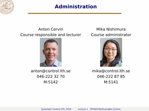
Administration
Anton Cervin Mika Nishimura
Course responsible and lecturer Course administrator
[email protected] [email protected]
046-222 32 70 046-222 87 85
M:5142 M:5141
Automatic Control LTH, 2019 Lecture 1 FRTN10 Multivariable Control
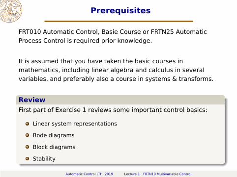
Prerequisites
FRT010 Automatic Control, Basie Course or FRTN25 Automatic
Process Control is required prior knowledge.
It is assumed that you have taken the basic courses in
mathematics, including linear algebra and calculus in several
variables, and preferably also a course in systems & transforms.
Automatic Control LTH, 2019 Lecture 1 FRTN10 Multivariable Control
Prerequisites
FRT010 Automatic Control, Basie Course or FRTN25 Automatic
Process Control is required prior knowledge.
It is assumed that you have taken the basic courses in
mathematics, including linear algebra and calculus in several
variables, and preferably also a course in systems & transforms.
Review
First part of Exercise 1 reviews some important control basics:
Linear system representations
Bode diagrams
Block diagrams
Stability
Automatic Control LTH, 2019 Lecture 1 FRTN10 Multivariable Control

Course material
All course material is available in English. Lecture slides, lecture
notes, exercise problems, and laboratory assignments are
provided on the course homepage
http://www.control.lth.se/course/FRTN10
Lecture slides (also printed and handed out)
Lecture notes
Exercise problems with solutions
Laboratory assignments
Automatic Control—Collection of Formulae
Old exams
Automatic Control LTH, 2019 Lecture 1 FRTN10 Multivariable Control

Reading material
Optional reading is provided in Glad & Ljung: Regler-
teori – Flervariabla och olinjära metoder (Studentlitter-atur, 2003) / Control Theory – Multivariable and Nonlin-ear Methods (Taylor & Francis / CRC, 2000, also avail-able as e-book through Lund University Libraries)
A very good online resource for reviewing many of thebasic concepts of automatic control is Feedback Sys-
tems: An Introduction to Scientists and Engineers byKarl Johan Åström and Richard Murray
Automatic Control LTH, 2019 Lecture 1 FRTN10 Multivariable Control

Lectures
The lectures (30 hours in total) are given by Anton Cervin on
Mondays, Tuesdays, and Thursdays.
See the LTH schedule generator for details.
Automatic Control LTH, 2019 Lecture 1 FRTN10 Multivariable Control
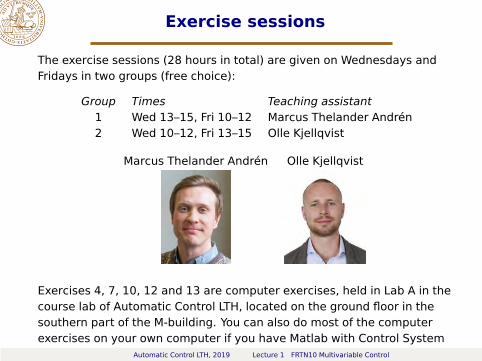
Exercise sessions
The exercise sessions (28 hours in total) are given on Wednesdays andFridays in two groups (free choice):
Group Times Teaching assistant
1 Wed 13–15, Fri 10–12 Marcus Thelander Andrén2 Wed 10–12, Fri 13–15 Olle Kjellqvist
Marcus Thelander Andrén Olle Kjellqvist
Exercises 4, 7, 10, 12 and 13 are computer exercises, held in Lab A in thecourse lab of Automatic Control LTH, located on the ground floor in thesouthern part of the M-building. You can also do most of the computerexercises on your own computer if you have Matlab with Control SystemToolbox installed.Automatic Control LTH, 2019 Lecture 1 FRTN10 Multivariable Control

Laboratory experiments
The three laboratory sessions (12 hours in total) are mandatory. Bookingis done in SAM. You must sign up before the first session starts. Beforeeach session there are pre-lab assignments that must be completed. Noreports are required afterwards.
Lab Weeks Booking Room Responsible Process
1 38–39 Sep 5 Lab C Marcus Thelander Andrén Flexible linear servo2 40–41 Sep 16 Lab C Olle Kjellqvist Quadruple tank3 42–43 Sep 30 Lab B Nils Vreman MinSeg
Automatic Control LTH, 2019 Lecture 1 FRTN10 Multivariable Control

Exam
The exam is given on Tuesday October 29 at 08:00–13:00 in
Vic3:B-C.
Retake exams are offered in January (unofficial) and April (official).
Lecture slides (with markings/small notes), lecture notes and the
Glad & Ljung book are allowed on the exam. You may also bring
Automatic Control—Collection of Formulae, standard mathematical
tables (e.g., TEFYMA), and a pocket calculator.
Automatic Control LTH, 2019 Lecture 1 FRTN10 Multivariable Control

Matlab
Matlab is used in the laboratory sessions as well as in the five
computer exercise sessions
Control System Toolbox
Simulink
CVX (http://cvxr.com/cvx), used in exercise session 12
Automatic Control LTH, 2019 Lecture 1 FRTN10 Multivariable Control
Feedback and Q&A
Feedback mechanisms for improving the course:
CEQ (reporting / longer time scale)
Student representatives (short time scale)
Election of student representatives ("kursombud")
Mid-course evaluation
We will use Piazza for Q&A. Take the opportunity to give and take
feedback!
Automatic Control LTH, 2019 Lecture 1 FRTN10 Multivariable Control

CEQ 2017, 2018
Automatic Control LTH, 2019 Lecture 1 FRTN10 Multivariable Control
Course registration
Please do the course registration in Ladok as soon as possible!
If you have not signed up for the course in advance, you need
to contact your program planner for late sign-up
If you have taken the course before and need to be
re-registered, send an email to [email protected]
Automatic Control LTH, 2019 Lecture 1 FRTN10 Multivariable Control
L1: Introduction
1 Course program
2 Course introduction
3 Signals and systems
Automatic Control LTH, 2019 Lecture 1 FRTN10 Multivariable Control

Multivariable control – Example 1
Automatic Control LTH, 2019 Lecture 1 FRTN10 Multivariable Control
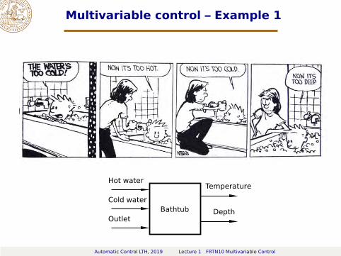
Multivariable control – Example 1
Bathtub
Hot water
Cold water
Outlet
Temperature
Depth
Automatic Control LTH, 2019 Lecture 1 FRTN10 Multivariable Control

Example 2: Rollover control
Automatic Control LTH, 2019 Lecture 1 FRTN10 Multivariable Control

Example 2: Rollover control
Vehicle
brake forces
steering angle
lateral velocity
yaw rate
Automatic Control LTH, 2019 Lecture 1 FRTN10 Multivariable Control
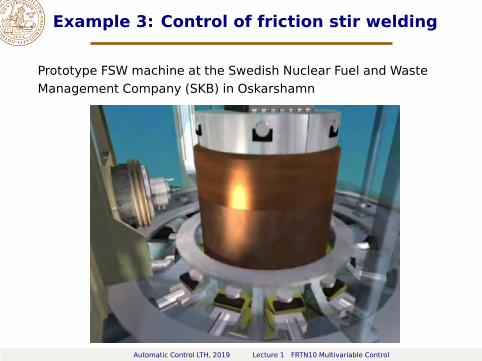
Example 3: Control of friction stir welding
Prototype FSW machine at the Swedish Nuclear Fuel and Waste
Management Company (SKB) in Oskarshamn
Automatic Control LTH, 2019 Lecture 1 FRTN10 Multivariable Control

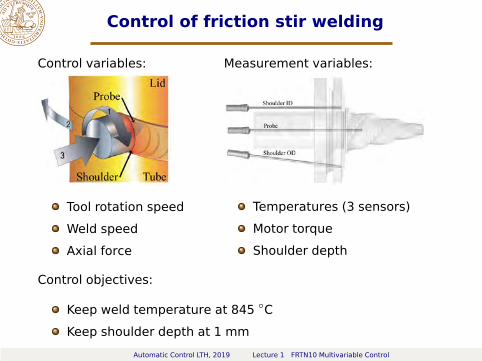
Control of friction stir welding
Control variables:
Tool rotation speed
Weld speed
Axial force
Measurement variables:
Temperatures (3 sensors)
Motor torque
Shoulder depth
Automatic Control LTH, 2019 Lecture 1 FRTN10 Multivariable Control
Control of friction stir welding
Control variables:
Tool rotation speed
Weld speed
Axial force
Measurement variables:
Temperatures (3 sensors)
Motor torque
Shoulder depth
Control objectives:
Keep weld temperature at 845 ◦C
Keep shoulder depth at 1 mm
Automatic Control LTH, 2019 Lecture 1 FRTN10 Multivariable Control

A general control system
[Boyd et al.: “Linear Controller Design: Limits of Performance via Convex
Optimization”, Proceedings of the IEEE, 78:3, 1990]Automatic Control LTH, 2019 Lecture 1 FRTN10 Multivariable Control

The control design process
Experiment
Implementation
Synthesis
Analysis
Matematical modeland
specification
Idea/Purpose
Automatic Control LTH, 2019 Lecture 1 FRTN10 Multivariable Control
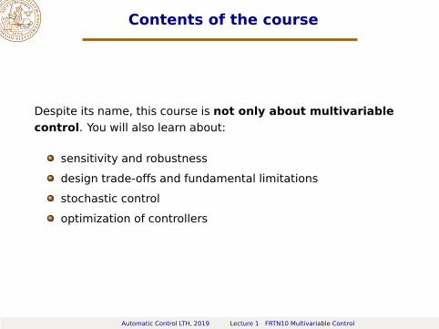
Contents of the course
Despite its name, this course is not only about multivariable
control. You will also learn about:
sensitivity and robustness
design trade-offs and fundamental limitations
stochastic control
optimization of controllers
Automatic Control LTH, 2019 Lecture 1 FRTN10 Multivariable Control
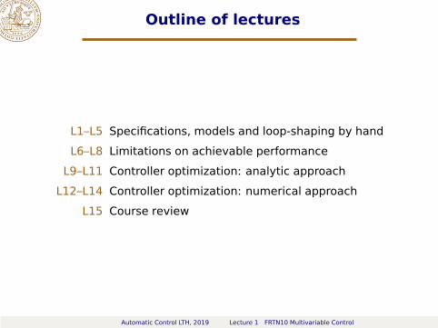
Outline of lectures
L1–L5 Specifications, models and loop-shaping by hand
L6–L8 Limitations on achievable performance
L9–L11 Controller optimization: analytic approach
L12–L14 Controller optimization: numerical approach
L15 Course review
Automatic Control LTH, 2019 Lecture 1 FRTN10 Multivariable Control

L1: Introduction
u y
S
Automatic Control LTH, 2019 Lecture 1 FRTN10 Multivariable Control
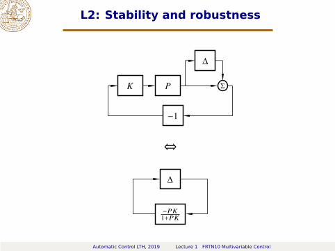
L2: Stability and robustness
replacements
ΣK P
∆
−1
⇔
∆
−PK1+PK
Automatic Control LTH, 2019 Lecture 1 FRTN10 Multivariable Control

L3: Specifications and disturbance models
F K P
−1
ΣΣΣr e u
w
z
v
y
0 10−1
0
1
Covariance
0.01 1
0.1
10
Spectrum
0 50
−2
0
2
Output
1
Automatic Control LTH, 2019 Lecture 1 FRTN10 Multivariable Control
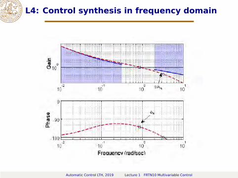
L4: Control synthesis in frequency domain
Automatic Control LTH, 2019 Lecture 1 FRTN10 Multivariable Control
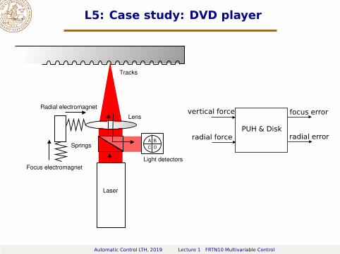
L5: Case study: DVD player
Radial electromagnet
Focus electromagnet
Springs
Light detectors
Laser
A B
C D
Tracks
Lens
PUH & Disk
vertical force
radial force
focus error
radial error
Automatic Control LTH, 2019 Lecture 1 FRTN10 Multivariable Control

L6: Controllability/observability, multivar. poles/zeros
u1u1
u2 u2x1
x1
x2
2x2
G(s) =
1
s + 21
2
s + 21
Automatic Control LTH, 2019 Lecture 1 FRTN10 Multivariable Control
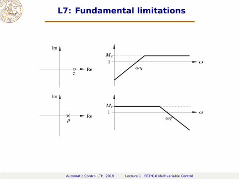
L7: Fundamental limitations
1
1
Im
Im
Re
Re
z
p
ω
ω
Ms
Mt
ωS
ωT
Automatic Control LTH, 2019 Lecture 1 FRTN10 Multivariable Control

L8: Decentralized control
Process
C1
C2
C3
u1
u2
u3
y1
y2
y3
Automatic Control LTH, 2019 Lecture 1 FRTN10 Multivariable Control

L9: Linear-quadratic control
replacements
P−
L
x
u z
minL
∫ ∞
0
(xTQ1x + uTQ2u
)dt
Automatic Control LTH, 2019 Lecture 1 FRTN10 Multivariable Control
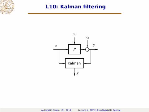
L10: Kalman filtering
P
Kalman
u y
x̂
v1v2
Automatic Control LTH, 2019 Lecture 1 FRTN10 Multivariable Control

L11: LQG control
P
Kalman
Lx̂
u
−
y
v1v2
minK,L
Ev1,v2
{xTQ1x + uTQ2u
}
Automatic Control LTH, 2019 Lecture 1 FRTN10 Multivariable Control
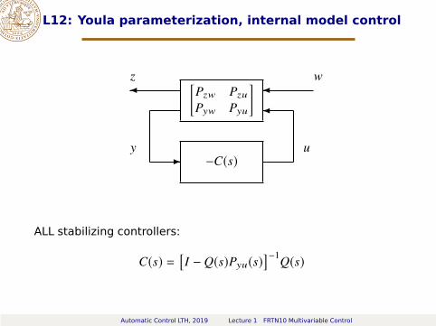
L12: Youla parameterization, internal model control
[Pzw Pzu
Pyw Pyu
]
−C(s)
✛ ✛
✛
✲
u
z
y
w
ALL stabilizing controllers:
C(s) =[I − Q(s)Pyu(s)
]−1Q(s)
Automatic Control LTH, 2019 Lecture 1 FRTN10 Multivariable Control

L13: Synthesis by convex optimization
Minimize
∫ ∞
−∞
|Pzw(iω) + Pzu(iω)
Q(iω)︷ ︸︸ ︷∑
k
Qkφk(iω) Pyw(iω)|2dω
subject to constraintsStep Response
Time (sec)
Am
plit
ude
0 1 2 3 4 5 6 7 8 9 10−0.1
−0.05
0
0.05
0.1
0.15
0.2
0.25
0.3
0.35
0.4
Bode Magnitude Diagram
Frequency (rad/sec)
Magnitude (
abs)
100
101
10−2
10−1
100
101
Automatic Control LTH, 2019 Lecture 1 FRTN10 Multivariable Control
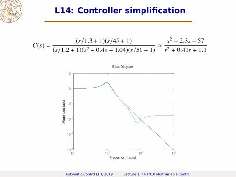
L14: Controller simplification
C(s) =(s/1.3 + 1)(s/45 + 1)
(s/1.2 + 1)(s2+ 0.4s + 1.04)(s/50 + 1)
≈s2 − 2.3s + 57
s2+ 0.41s + 1.1
10−1
100
101
102
10−4
10−3
10−2
10−1
100
101
Magnitude (
abs)
Bode Diagram
Frequency (rad/s)
Automatic Control LTH, 2019 Lecture 1 FRTN10 Multivariable Control

L1: Introduction
1 Course program
2 Course introduction
3 Signals and systems
System representations
Signal norm and system gain
Automatic Control LTH, 2019 Lecture 1 FRTN10 Multivariable Control

Systems
u y
S
A system is a mapping from the input signal u(t) to the
output signal y(t), −∞ < t < ∞:
y = S(u)
Automatic Control LTH, 2019 Lecture 1 FRTN10 Multivariable Control

System properties
A system S is
causal if y(t1) only depends on u(t), −∞ < t ≤ t1,
non-causal otherwise
static if y(t1) only depends on u(t1),
dynamic otherwise
discrete-time if u(t) and y(t) are only defined for a countable
set of discrete time instances t = tk, k = 0,±1,±2, . . .,
continuous-time otherwise
Automatic Control LTH, 2019 Lecture 1 FRTN10 Multivariable Control
System properties (cont’d)
A system S is
single-variable or scalar if u(t) and y(t) are scalar signals,
multivariable otherwise
time-invariant if y(t) = S(u(t)) implies y(t + τ) = S(u(t + τ)),
time-varying otherwise
linear if S(α1u1 + α2u2) = α1S(u1) + α2S(u2),
nonlinear otherwise
Automatic Control LTH, 2019 Lecture 1 FRTN10 Multivariable Control
LTI system representations
We will mainly deal with continuous-time linear time-invariant
(LTI) systems in this course
For LTI systems, the same input–output mapping S can be
represented in a number of equivalent ways:
linear ordinary differential equation
linear state-space model
transfer function
impulse response
step response
frequency response
. . .
Automatic Control LTH, 2019 Lecture 1 FRTN10 Multivariable Control

State-space models
u y
x
S
Linear state-space model:
{Ûx = Ax + Bu
y = Cx + Du
Solution:
y(t) = CeAt x(0) +
∫t
0
CeA(t−τ)Bu(τ)dτ + Du(t)
Automatic Control LTH, 2019 Lecture 1 FRTN10 Multivariable Control
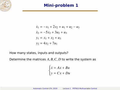
Mini-problem 1
Ûx1 = −x1 + 2x2 + u1 + u2 − u3
Ûx2 = −5x2 + 3u2 + u3
y1 = x1 + x2 + u3
y2 = 4x2 + 7u1
How many states, inputs and outputs?
Determine the matrices A, B,C,D to write the system as
{Ûx = Ax + Bu
y = Cx + Du
Automatic Control LTH, 2019 Lecture 1 FRTN10 Multivariable Control
Mini-problem 1
Automatic Control LTH, 2019 Lecture 1 FRTN10 Multivariable Control

Change of coordinates
{Ûx = Ax + Bu
y = Cx + Du
Change of coordinates
z = T x, T invertible
{Ûz = T Ûx = T(Ax + Bu) = T(AT−1z + Bu) = TAT−1z + TBu
y = Cx + Du = CT−1z + Du
There are infinitely many different state-space representations of
the same input–output mapping y = S(u)Automatic Control LTH, 2019 Lecture 1 FRTN10 Multivariable Control
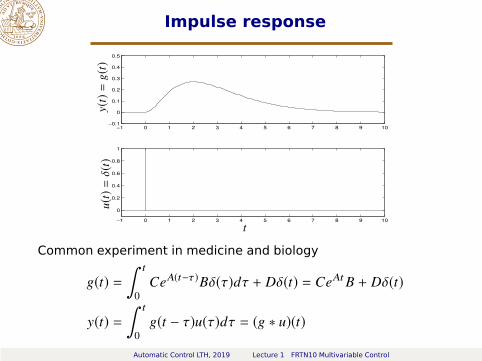
Impulse response
−1 0 1 2 3 4 5 6 7 8 9 10
0
0.2
0.4
0.6
0.8
1
−1 0 1 2 3 4 5 6 7 8 9 10−0.1
0
0.1
0.2
0.3
0.4
0.5
y(t)=g(t)
u(t)=δ(t)
t
Common experiment in medicine and biology
g(t) =
∫t
0
CeA(t−τ)Bδ(τ)dτ + Dδ(t) = CeAtB + Dδ(t)
y(t) =
∫t
0
g(t − τ)u(τ)dτ = (g ∗ u)(t)
Automatic Control LTH, 2019 Lecture 1 FRTN10 Multivariable Control
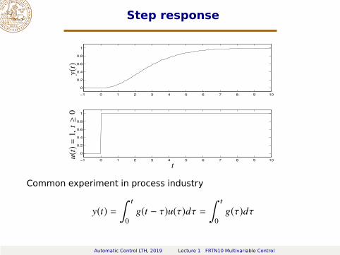
Step response
−1 0 1 2 3 4 5 6 7 8 9 10
0
0.2
0.4
0.6
0.8
1
−1 0 1 2 3 4 5 6 7 8 9 10
0
0.2
0.4
0.6
0.8
1
y(t)
u(t)=
1,t≥
0
t
Common experiment in process industry
y(t) =
∫t
0
g(t − τ)u(τ)dτ =
∫t
0
g(τ)dτ
Automatic Control LTH, 2019 Lecture 1 FRTN10 Multivariable Control
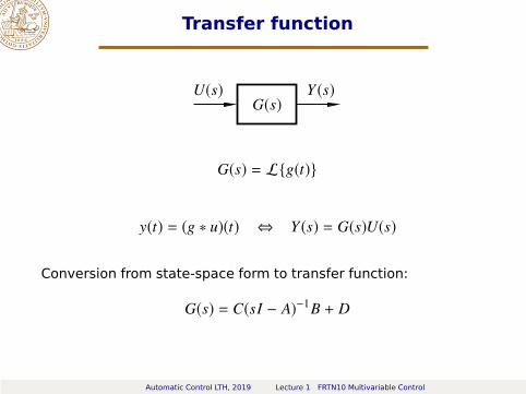
Transfer function
U(s) Y (s)G(s)
G(s) = L{g(t)}
y(t) = (g ∗ u)(t) ⇔ Y (s) = G(s)U(s)
Conversion from state-space form to transfer function:
G(s) = C(sI − A)−1B + D
Automatic Control LTH, 2019 Lecture 1 FRTN10 Multivariable Control
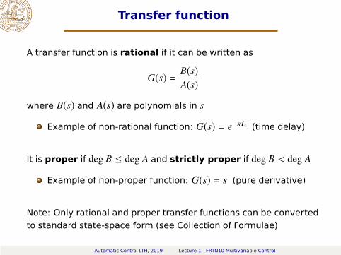
Transfer function
A transfer function is rational if it can be written as
G(s) =B(s)
A(s)
where B(s) and A(s) are polynomials in s
Example of non-rational function: G(s) = e−sL (time delay)
It is proper if deg B ≤ deg A and strictly proper if deg B < deg A
Example of non-proper function: G(s) = s (pure derivative)
Note: Only rational and proper transfer functions can be converted
to standard state-space form (see Collection of Formulae)
Automatic Control LTH, 2019 Lecture 1 FRTN10 Multivariable Control
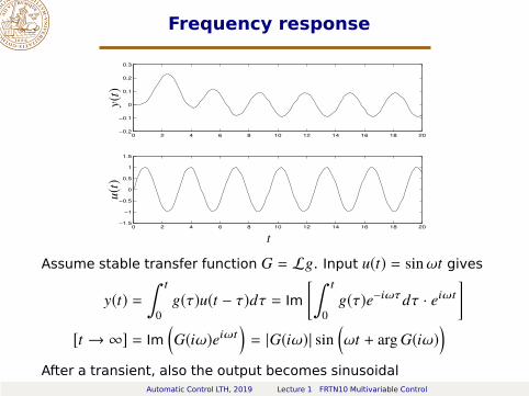
Frequency response
0 2 4 6 8 10 12 14 16 18 20−0.2
−0.1
0
0.1
0.2
0.3
0 2 4 6 8 10 12 14 16 18 20−1.5
−1
−0.5
0
0.5
1
1.5
y(t)
u(t)
t
Assume stable transfer function G = Lg. Input u(t) = sinωt gives
y(t) =
∫t
0
g(τ)u(t − τ)dτ = Im
[∫t
0
g(τ)e−iωτdτ · eiωt
]
[t → ∞] = Im
(G(iω)eiωt
)= |G(iω)| sin
(ωt + arg G(iω)
)
After a transient, also the output becomes sinusoidal
Automatic Control LTH, 2019 Lecture 1 FRTN10 Multivariable Control
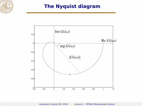
The Nyquist diagram
−0.4 −0.2 0 0.2 0.4 0.6 0.8 1 1.2−1
−0.8
−0.6
−0.4
−0.2
0
0.2
arg G(iω)
|G(iω)|
Im G(iω)
Re G(iω)
Automatic Control LTH, 2019 Lecture 1 FRTN10 Multivariable Control

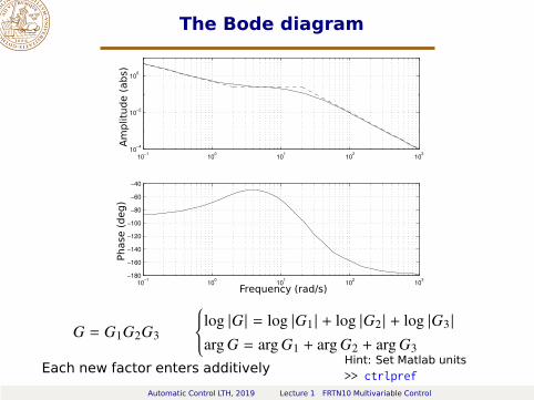
The Bode diagram
10−1
100
101
102
103
10−4
10−2
100
10−1
100
101
102
103
−180
−160
−140
−120
−100
−80
−60
−40
Amplitude(abs)
Phase(deg)
Frequency (rad/s)
G = G1G2G3
{log |G | = log |G1 | + log |G2 | + log |G3 |
arg G = arg G1 + arg G2 + arg G3
Each new factor enters additively
Automatic Control LTH, 2019 Lecture 1 FRTN10 Multivariable Control
The Bode diagram
10−1
100
101
102
103
10−4
10−2
100
10−1
100
101
102
103
−180
−160
−140
−120
−100
−80
−60
−40
Amplitude(abs)
Phase(deg)
Frequency (rad/s)
G = G1G2G3
{log |G | = log |G1 | + log |G2 | + log |G3 |
arg G = arg G1 + arg G2 + arg G3
Each new factor enters additivelyHint: Set Matlab units
>> ctrlpref
Automatic Control LTH, 2019 Lecture 1 FRTN10 Multivariable Control

Signal norm and system gain
PSfrag replacements
u y
S
How to quantify
the “size” of the signals u and y
the “maximum amplification” between u and y
Automatic Control LTH, 2019 Lecture 1 FRTN10 Multivariable Control

Signal norm
The L2 norm of a signal y(t) ∈ Rn is defined as
‖y‖ =
√∫ ∞
0
|y(t)|2dt
By Parseval’s theorem it can also be expressed as
‖y‖ =
√1
2π
∫ ∞
−∞
|Y (iω)|2dω
Automatic Control LTH, 2019 Lecture 1 FRTN10 Multivariable Control
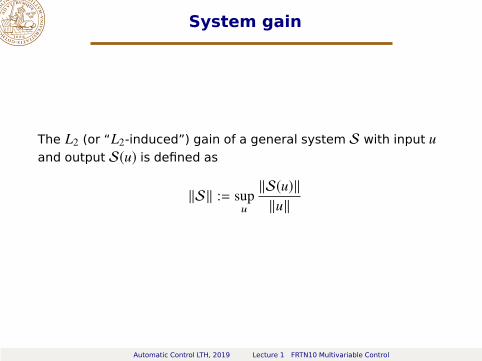
System gain
The L2 (or “L2-induced”) gain of a general system S with input u
and output S(u) is defined as
‖S‖ := supu
‖S(u)‖
‖u‖
Automatic Control LTH, 2019 Lecture 1 FRTN10 Multivariable Control

L2 gain of LTI systems
Theorem 1.1
Consider a stable LTI system S with transfer function G(s). Then
‖S‖ = supω
|G(iω)| := ‖G‖∞
Proof. Let y = S(u). Then
‖y‖2=
1
2π
∫ ∞
−∞
|Y (iω)|2dω =1
2π
∫ ∞
−∞
|G(iω)|2 |U(iω)|2dω ≤ ‖G‖2∞‖u‖2
The inequality is arbitrarily tight when u(t) is a sinusoid near the
maximizing frequency.
(How to interpret |G(iω)| for matrix transfer functions will be explained in
Lecture 2.)
Automatic Control LTH, 2019 Lecture 1 FRTN10 Multivariable Control
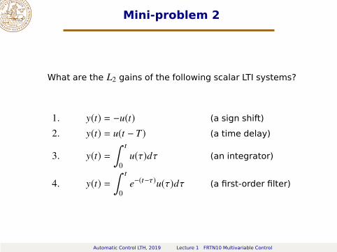
Mini-problem 2
What are the L2 gains of the following scalar LTI systems?
1. y(t) = −u(t) (a sign shift)
2. y(t) = u(t − T) (a time delay)
3. y(t) =
∫t
0
u(τ)dτ (an integrator)
4. y(t) =
∫t
0
e−(t−τ)u(τ)dτ (a first-order filter)
Automatic Control LTH, 2019 Lecture 1 FRTN10 Multivariable Control

Mini-problem 2
Automatic Control LTH, 2019 Lecture 1 FRTN10 Multivariable Control

Summary of Lecture 1
Course overview
Review of LTI system descriptions (see also Exercise 1)
L2 norm of signals
Definition: ‖y‖ :=
√∫ ∞
0|y(t)|2dt
L2 gain of systems
Definition: ‖S‖ := supu‖S(u) ‖‖u ‖
Special case—stable LTI systems: ‖S‖ = supω|G(iω)| := ‖G‖∞
(also known as the “H∞ norm” of the system)
Automatic Control LTH, 2019 Lecture 1 FRTN10 Multivariable Control