Distortions in Perceived Direction of Motion Predicted by Population Response in 

Visual Cortex 

by 

Wei Wu 

Department of Neurobiology Duke University 

 

Date:_______________________ Approved: 

 ___________________________ David Fitzpatrick, Supervisor 

 ___________________________ 

Michael Platt, Chair  

___________________________ Richard Mooney 

 ___________________________ 

Paul Tiesinga  

Dissertation submitted in partial fulfillment of the requirements for the degree of Doctor  

of Philosophy in the Department of Neurobiology in the Graduate School 

of Duke University  

2009  

 

 

 

ABSTRACT 

Distortions in Perceived Direction of Motion Predicted by Population Response in 

Visual Cortex 

by 

Wei Wu 

Department of Neurobiology Duke University 

 

Date:_______________________ Approved: 

 ___________________________ David Fitzpatrick, Supervisor 

 ___________________________ 

Michael Platt, Chair  

___________________________ Richard Mooney 

 ___________________________ 

Paul Tiesinga  

 

An abstract of a dissertation submitted in partial fulfillment of the requirements for the degree of Doctor of Philosophy in the Department of 

Neurobiology in the Graduate School of Duke University 

 2009 

 

 

 

                                    

Copyright by Wei Wu 2009  

 

 

iv

Abstract  

The visual system is thought to represent the trajectory of moving objects in the activity 

of large populations of cortical neurons that respond preferentially to the direction of 

stimulus motion. Here I employed in vivo voltage sensitive dye (VSD) imaging to 

explore how abrupt changes in the trajectory of a moving stimulus impact the 

population coding of motion direction in ferret primary visual cortex (V1). For motion in 

a constant direction, the peak of the cortical population response reliably signaled the 

stimulus trajectory; but for abrupt changes in motion direction, the peak of the 

population response departed significantly from the stimulus trajectory in a fashion that 

depended on the size of the direction deviation. For small direction deviation angles, the 

peak of the active population shifted from values consistent with the initial direction of 

motion to those consistent with the final direction of motion by progressing smoothly 

through intermediate directions not present in the stimulus.  In contrast, for large 

direction deviation angles, peak values consistent with the initial motion direction were 

followed by: a small deviation away from the final motion direction, a rapid 180° jump, 

and a gradual shift to the final direction. These departures of the population response 

from the actual trajectory of the stimulus predict specific misperceptions of motion 

direction that were confirmed by human psychophysical experiments. I conclude that 

 

 

v

cortical dynamics and population coding mechanisms combine to place constraints on 

the accuracy with which abrupt changes in direction of motion can be represented by 

cortical circuits. 

 

 

vi

Contents

Abstract ......................................................................................................................................... iv 

List of Figures ................................................................................................................................ x 

Acknowledgements .................................................................................................................... xii 

Chapter 1: Introduction ................................................................................................................ 1 

1.1 Overview ........................................................................................................................... 1 

1.2 The realm of adaptation .................................................................................................. 2 

1.2.1 Tilt aftereffect (TAE) and direction aftereffect (DAE) ............................................ 2 

1.2.2 Orientation adaptation ............................................................................................... 3 

1.2.3 Direction adaptation ................................................................................................... 6 

1.3 Population response ......................................................................................................... 7 

1.3.1 Sparse coding and population coding ...................................................................... 8 

1.3.2 Advantage of population coding ............................................................................ 10 

1.4 From tuning curves to population response .............................................................. 11 

1.4.1 Gap between tuning curves and population response ........................................ 12 

1.4.2 Does alteration in population response necessarily involve changes of tuning curves? ................................................................................................................................. 15 

1.5 Voltage‐sensitive dye imaging: a direct measure of the population response ...... 16 

1.6 Aim and scope of present study ................................................................................... 18 

Chapter 2: Capturing and decoding the dynamics of population responses to changes of motion direction .......................................................................................................................... 28 

2.1 Introduction ..................................................................................................................... 28 

 

 

vii

2.2 Results .............................................................................................................................. 29 

2.2.1 The dynamics of the population response to motion transition in primary visual cortex vary as a function of direction deviation angle ...................................... 29 

2.2.2 The spike discharge population response constructed from unit recording data is consistent with VSDI measurements ........................................................................... 33 

2.3 Summary .......................................................................................................................... 36 

2.4 Materials and methods .................................................................................................. 36 

2.4.1 Animal preparation ................................................................................................... 37 

2.4.2 Intrinsic signal optical imaging ............................................................................... 38 

2.4.3 Voltage‐sensitive dye imaging (VSDI) ................................................................... 40 

2.4.4 VSDI data analysis .................................................................................................... 41 

2.4.5 Electrophysiology ...................................................................................................... 44 

Chapter 3: Mechanism of population response to changes in motion direction: linearity vs non‐linearity ............................................................................................................................ 66 

3.1 Introduction ..................................................................................................................... 66 

3.2 Results .............................................................................................................................. 67 

3.2.1 A linear combination model explains certain aspects of the population response to rapid changes in motion direction .............................................................. 67 

3.2.2 Additional nonlinear mechanisms shape the dynamics of population response ............................................................................................................................................... 70 

3.3 Summary .......................................................................................................................... 71 

3.4 Materials and methods .................................................................................................. 72 

3.4.1 Linear combination model ....................................................................................... 72 

3.4.2 VSDI experiment to test the linearity ..................................................................... 73 

 

 

viii

Chapter 4: Perceptual distortions in motion trajectory ......................................................... 86 

4.1 Introduction ..................................................................................................................... 86 

4.2 Results .............................................................................................................................. 87 

4.2.1 Distortions in perceived motion trajectory accord with the dynamics of the population response ........................................................................................................... 87 

4.2.2 The perception distortion for motion trajectory could not be explained by positional information ....................................................................................................... 89 

4.3 Summary .......................................................................................................................... 91 

4.4 Materials and methods .................................................................................................. 91 

4.4.1 Experiment 1: Measure the distortion of motion transition perception. ........... 91 

4.4.2 Experiment 2: Measure the noise of position judgment at different eccentricities and reconstruct motion trajectory using positional information. ........ 95 

Chapter 5: Discussion ............................................................................................................... 112 

5.1 Relationship to earlier studies .................................................................................... 112 

5.1.1 Dynamics of population response to motion transition .................................... 112 

5.1.2 Distortions of motion direction perception induced by stimulus context ...... 117 

5.2 The combination of the cortical dynamics and population coding mechanisms places constraints on stimulus representation ............................................................... 122 

5.2.1 Key components that accounts for the distortions in motion direction representation ................................................................................................................... 122 

5.2.2 Interaction between population coding and cortical dynamics in other visual attributes ............................................................................................................................ 124 

5.2.3 Interaction between population coding and cortical dynamics in other sensory modalities .......................................................................................................................... 127 

5.3 Limitations and future directions ............................................................................... 130 

 

 

ix

5.3.1 Sources of VSD signals ........................................................................................... 130 

5.3.2 Contribution of different neurons to the population response ......................... 132 

5.3.3 Methods to decode the population response profile .......................................... 133 

5.3.4 Interpretation of the human psychophysical data .............................................. 135 

5.4 Conclusion ..................................................................................................................... 136 

References .................................................................................................................................. 138 

Biography ................................................................................................................................... 149 

 

 

 

x

List of Figures Figure 1:  Adaptation‐induced plasticity of orientation tuning in V1 neurons. ................. 20 

Figure 2:  Direction‐induced plasticity of direction tuning in MT neurons. ...................... 22 

Figure 3:  A neural implementation of a maximum likelihood estimator. ......................... 24 

Figure 4: Predicting the impact of tuning curve properties on population response using a population coding model. ....................................................................................................... 26 

Figure 5: The population response to a constant motion stimulus in ferret primary visual cortex. ............................................................................................................................................ 46 

Figure 6: Visual stimuli and difference image analysis. ........................................................ 48 

Figure 7: The population response to motion transitions with different direction deviation angles in ferret primary visual cortex. ................................................................... 50 

Figure 8: Population response profile (PRP) analysis and decoding method for the peak direction and amplitude. ............................................................................................................ 52 

Figure 9: Dynamics of the population response to a constant motion stimulus in ferret primary visual cortex. ................................................................................................................. 54 

Figure 10: Dynamics of the population response to motion transition in ferret primary visual cortex vary as a function of direction deviation angle. .............................................. 56 

Figure 11: Dynamics of the population direction tuning function depend on direction deviation angle. ........................................................................................................................... 58 

Figure 12: Results obtained using PRP analysis on single condition images are similar to that obtained from difference images. ..................................................................................... 60 

Figure 13: Dynamics of the population response to changes of motion direction can be extrapolated from unit recording experiments. ...................................................................... 62 

Figure 14: The population response constructed from electrophysiological data is consistent with VSDI measurements. ....................................................................................... 64 

 

 

xi

Figure 15: A linear combination model explains certain aspects of the population response to motion transition. ................................................................................................... 74 

Figure 16: Dynamics of population response predicted by the linear combination model. ....................................................................................................................................................... 76 

Figure 17: Sensitivity test for two parameters in the linear combination model. .............. 78 

Figure 18: A direct test for linearity of the population response.......................................... 80 

Figure 19: Population responses demonstrate a nonlinearity that depends on direction deviation angles. ......................................................................................................................... 82 

Figure 20: Evidence for nonlinear dynamics during the transition period. ....................... 84 

Figure 21: A simple model to predict perceived trajectory. .................................................. 98 

Figure 22: The perceived trajectory predicted by VSD data. .............................................. 100 

Figure 23: Experimental paradigm to measure the distortion of human perception of changes in stimulus motion. .................................................................................................... 102 

Figure 24: Experimental results from an example subject. ................................................. 104 

Figure 25: Summary of the data from all subjects (n=4). ..................................................... 106 

Figure 26: The distortion of motion transition perception and perception of positional information at different eccentricities. ................................................................................... 108 

Figure 27: Reconstructed motion trajectories based on positional information exhibit no curvature bias that is consistent with the distortion of motion transition perception (data acquired at 5° eccentricity). ...................................................................................................... 110 

 

 

 

xii

Acknowledgements

I have the tremendous pleasure to work with many great people during my

graduate career. First, I would like to thank my advisor, David Fitzpatrick, for his

continuous guidance and support. David was involved in all the work presented in my

thesis. I have benefited greatly from his knowledge and clear thinking. David is also a

role model for me. Not only have I learned science from him, I also have learned how to

be a better person. I am sure that I will benefit from my experience in Fitzpatrick Lab for

a life time.

Next, I would like to thank my collaborators on the projects that are presented

here. Paul Tiesinga helped me to analyze the VSD data and build the linear combination

model. Thomas Tucker set up the VSDI experiment in the lab and also helped me to

collect the electrophysiological data. Stephen Mitroff provided guidance for the

psychophysical experiments. Julie Heiner helped me with the ferret surgery.

Then, I would like to thank current and former members of Fitzpatrick Lab. I had

a great time in the past six years in the lab. Thanks to Len White for providing numerous

helpful comments for my experimental data. Thanks to Elizabeth (Zab) Johnson for

giving me great help in every aspect. Thanks to Thomas Tucker for teaching me hand-

over-hand how to performance VSDI experiments. Thanks to Ye Li for helping me with

 

 

xiii

the ferret surgery and offering me a lot of encouragement and helpful suggestion. Thanks

to Steve Van Hooser for helping me with programming and equipment setup. Thanks to

Maria Christensson for providing many valuable inputs about my thesis, manuscripts and

presentations. Thanks to Julie Heiner for making everyone’s lab life much easier. Thanks

to Amit Basole for enlightening me in the early stage of my thesis work. Also thanks to

Sean MacEvoy, Mark Mazurek and Xiaoying Huang for their support.

I thank my committee member, Michael Platt, Richard Mooney, Nell Cant, Paul

Tiesinga for their guidance. Thanks to Dona Chikarashi, Guoping Feng and George

Augustine for supporting me continuously during my graduate career. I also want to

thank Jessica Herbst, Polly Garner and Ann Sink and the rest administrative staff. Thanks

to my graduate student peers Hao Zhang, Yulong Li, Zhonghua Lu and Huimeng Lei.

Finally, I would like to thank my parents and my fiancée Lixian Zhong for their

unconditional love and support, without which nothing will be possible.

 

1 

 

Chapter 1: Introduction

1.1 Overview

Encoding the trajectory of a moving stimulus that abruptly changes its direction 

of motion provides a particularly vivid example of the challenges inherent in using 

cortical circuits to represent rapidly changing stimulus features that are ubiquitous in 

visual scenes.  Instantaneous changes in the properties of a visual stimulus are 

accompanied by alterations in the activity of cortical circuits that begin with some delay 

and continue beyond the stimulus event for 100’s of milliseconds (Sharon and Grinvald, 

2002; Jancke et al., 2004). As a consequence, the cortical response to a stimulus that 

abruptly changes its direction of motion must involve a transition period during which 

the pattern of activity representing the initial direction of motion is replaced by the 

pattern of activity representing the new direction of motion. Given that the direction of 

stimulus motion is thought to be represented in visual cortex by the relative activity of a 

distributed population of neurons that are broadly tuned to direction of motion (Treue 

et al., 2000; Abbott, 1994; Pouget et al., 2003; Webb et al., 2007), this raises the question: 

Does the population response accurately track a stimulus that changes its direction of 

motion, or do the circuit dynamics that accompany changes in stimulus properties yield 

population representations that depart from the actual direction of stimulus motion, 

and, if so, how? 

 

2 

 

1.2 The realm of adaptation

The question of how prevailing stimulus conditions impact response to a new 

stimulus has traditionally been considered within the realm of adaptation—a temporary 

alteration in neuronal response that is induced by and outlasts a stimulus, and is 

thought to be the basis for distortions in visual perception such as the orientation tilt 

effect and the direction repulsion effect (Clifford, 2002). These effects typically have been 

studied with single unit recordings, which have revealed significant changes in response 

magnitude and shifts in tuning curves for stimulus features such as orientation and 

direction of motion (Muller et al., 1999; Dragoi et al., 2000; Dragoi et al., 2002; Felsen et 

al., 2002; Kohn and Movshon, 2004; Kohn, 2007).   The magnitude and direction of these 

changes have been shown to vary systematically as a function of stimulus conditions, 

and these observations suggest that the population response to stimulus transitions 

involves significant non‐linearities thus would lead to distortions in perception as a 

stimulus changes its direction of motion.   

1.2.1 Tilt aftereffect (TAE) and direction aftereffect (DAE)

Prolonged adaptation to an oriented pattern affects the perceived orientation of a 

subsequently observed pattern (Gibson and Radner, 1937), a phenomenon known as the 

tilt aftereffect (TAE). When the angular difference between adapting and test orientation 

is  small,  the  test  stimulus  appears  to  be  repelled  away  from  the  adapting  stimulus. 

 

3 

 

When the angular difference is large, the test stimulus will appear to be slightly attracted 

towards  the  adapting  stimulus  (Clifford,  2002).  The  direction  aftereffect  (DAE)  is  a 

motion  analogue  of  the  TAE.  Prolonged  exposure  to  a  moving  pattern  affects  the 

perceived direction of  subsequent motion  (Levinson  and  Sekuler,  1976; Patterson  and 

Becker, 1996; Phinney, 1997; Schrater and Simoncelli, 1998; Clifford, 2002). For angles up 

to  around  100  degrees  between  the  directions  of  motion  of  the  adapting  and  test 

patterns, the perceived direction of the test pattern tends to be repelled away from  the 

adapting  direction.  For  angles  larger  than  100  degrees  between  adapting  and  test 

directions,  the perceived direction of  the  test  tends  to be attracted  towards  that of  the 

adapter (Schrater and Simoncelli, 1998; Clifford, 2002).  

1.2.2 Orientation adaptation

Compared  to direction adaptation,  the neural basis of orientation adaptation  is 

more extensively studied and better understood. Since direction aftereffect shares many 

similarities with tilt aftereffect, understanding the neural basis of orientation adaptation 

might provide some insights into mechanisms of direction adaptation.  

Orientation adaptation  first occurs  in  the primary visual cortex.  It  is essentially 

absent  in  subcortical  neurons  (Ohzawa  et  al.,  1985;  Shou  et  al.,  1996).  The  most 

prominent  consequence of orientation adaptation  is  the  suppression of  cortical neural 

response.  Adaptation  to  an  orientation  pattern  has  been  shown  to  decrease  the 

 

4 

 

responsiveness of cortical neurons to their preferred orientations (Movshon and Lennie, 

1979). This  reduction shows orientation specificity, being strongest when  the adapting 

orientation and test orientation are identical. (Maffei et al., 1973; Carandini et al., 1998)  

However,  the reduction of neuronal activity  is not  the whole story.  It has been 

shown  that  orientation  adaptation  can  shift  the  peak  tuning  position  of  orientation 

selective neurons. Using  a  rapid  adaptation paradigm, Muller  et  al.  revealed  that  the 

peak orientation tuning position of complex cells in monkey primary visual cortex was 

affected by  the adapting  stimulus  (Muller et al., 1999). Adapting orientations near  the 

preferred  orientation  of  the  neuron  caused  a  repulsive  shift  of  the  orientation  tuning 

curve. This phenomena was also discovered in cat striate cortex by several other groups 

(Figure  1a,  Dragoi  et  al.,  2000;  Dragoi  et  al.,  2002;  Felson  et  al.,  2002;  but  also  see 

Ghisovan  et  al.,  2008).  The  magnitude  of  the  post‐adaptation  shift  in  the  preferred 

orientation depended on the angular difference between the adaptor and the preferred 

orientation  (Figure 1b, Dragoi et al., 2000). The  largest  repulsive shift was  found with 

small  angular  difference  (5°  to  22.5°).  Repulsive  shifts  in  V1  tuning  occur  after 

adaptation  as  brief  as  several  tens  or  hundreds  of milliseconds  (Dragoi  et  al.,  2002; 

Felson et al., 2002; Muller et al., 1999) or  lasting as  long as 20 min  (Dragoi et al., 2000, 

2001).  In  the most  systematic  exploration  of  the  role  of  adaptation  duration  to  date, 

Dragoi et al.  (Dragoi et al., 2000)  found  repulsive  shifts  in V1 orientation  tuning after 

 

5 

 

adaptation  ranging  in  duration  from  10s  to  10min with  the  latter  giving  rise  to  the 

strongest effects.  

Besides  the shift of  the peak orientation,  the  tuning curve also undergoes other 

changes after adaptation. After adaption  to  the orientation stimulus near  the preferred 

orientation, the responses on the flank of the tuning curve near the adapting orientation 

were depressed, whereas  responses on  the opposite  flank were  enhanced  (Figure 1a). 

Moreover,  the  orientation  selectivity  was  broadened  (Figure  1c).  In  contrast,  after 

adaption  to  the  orthogonal  orientation,  neurons  showed  a  sharpening  in  orientation 

tuning (Figure 1c), along with an increase in responsiveness (Dragoi et al., 2000; Dragoi 

et al., 2002). 

The capacity for neurons to display orientation plasticity induced by adaptation 

was shown to be different across the cortex (Dragoi et al., 2001). Compared to neurons 

located  in  iso‐orientation domains, neurons located at and near pinwheel centers show 

larger repulsive shifts in orientation preference after adaptation. A possible explanation 

for  these  phenomena  is  that  neurons  in  pinwheel  centers  receive  inputs  from  a 

population of cortical neurons with a broader range of orientations (Marino et al., 2005); 

thus  altering  the  efficacy  of  these  inputs  through  adaptation  is  likely  to  induce more 

profound changes  in  the orientation preference of neurons at or near pinwheel centers 

(Dragoi et al., 2001).  

 

6 

 

1.2.3 Direction adaptation

The impact of direction adaptation has been studied in two visual cortical areas: 

primary visual cortex  (V1) and middle  temporal visual area  (MT). Orderly distributed 

direction maps have been  shown  in primary visual  cortex of  the  ferret  (Weliky  et al., 

1996).  Responsiveness  of  neurons  in  primary  visual  cortex  is modulated  by motion 

adaptation.  This modulation  is  direction‐specific.  Prolonged  adaptation with  gratings 

drifting  continuously  in  the  preferred  directions  suppressed  the  responsiveness  of 

cortical  neurons  significantly  (Vautin  and  Berkley,  1977;  von  der Heydt  et  al.,  1978; 

Hammond et al., 1985). Gratings drifting  in directions nearby  the preferred directions 

reduced  the neuronal  responsiveness  to  a  lesser  extent  (Hammond  et  al.,  1989) while 

gratings  drifting  in  the  null  directions  had  no  effect  or  slightly  enhanced  neuronal 

responsiveness (von der Heydet et al., 1978; Marlin et al., 1988; Giaschi et al., 1993).  

Does  motion adaptation shift the peak of the tuning curve of direction selective 

neurons? Kohn and Movshon recorded 40 neurons from V1. After flank adaptation (i.e., 

the adaptor’s direction is on the flank of the neuron’s preferred direction), no significant 

shifts were detected. However,  they  found direction  tuning curves  in MT were shifted 

by motion adaptation systematically  (Kohn and Movshon, 2004). MT  is an extrastriate 

area containing a high proportion of direction‐selective cells (Zeki, 1974; Maunsell and 

Van Essen, 1983) and has a  clearly established  role  in  the perception of visual motion 

 

7 

 

(Newsome et al., 1989). Experiments have shown that motion adaptation can modulate 

the  responsiveness  of  MT  neurons.  Responses  of  MT  neurons  to  motion  in  their 

preferred direction were reduced by adaptation to motion in the preferred direction and 

enhanced by prolonged adaptation in the opposite direction (Petersen et al., 1985; Priebe 

et al., 2002).  

Kohn  and  Movshon  found  that  adaptation  to  a  prolonged  drifting  grating 

moving  in  near‐preferred  directions  caused  an  attractive  shift  of  the  tuning  curves, 

which  is  in  the opposite direction  to  the shift effect  induced by orientation adaptation 

(Figure 2a and Figure 2b, Kohn and Movshon, 2004). Response amplitude and cellular 

tuning width were  also  changed  by  direction  adaptation.  Response  to  test  direction 

stimuli well‐matched to the adapter were maintained best, but other test stimuli evoked 

much  weaker  responses  after  adaptation.  Meanwhile,  the  direction  tuning  after 

adaptation became significantly narrower (Figure 2c). Interestingly, both changes were 

in the opposite direction to what had been shown by the orientation adaptation studies. 

The  factors  that  account  for  the differences between  these  two  lines  of  studies  is  still 

unknown. 

1.3 Population response

As  mentioned  previously,  orientation  adaptation  and  direction  adaptation 

change neuronal tuning curves in a systematic fashion. How do these changes in tuning 

 

8 

 

curves  affect  perception?  In  order  to  address  this  question,  I  need  to  introduce  the 

concept  of  population  response,  which  is  believed  to  be  the  bridge  between  single 

neuron behavior and perception.  

1.3.1 Sparse coding and population coding

The sensory system receives huge amount of information from the environment 

constantly. How does the brain encode this flood of information in order to form useful 

internal representations to mediate behavior? Scientists have proposed and found 

evidence for two encoding strategies: sparse coding and population coding (Barlow, 

1972; Gross et al., 1969; Konorski, 1967; Logothetis and Sheinberg, 1996; Young and 

Yamane, 1992). 

Sparse coding is a neural encoding strategy in which information is represented 

by a relatively small fraction of simultaneously active neurons out of a large population. 

A famous example of sparse coding is the response of neurons in visual areas of the 

temporal lobe  to one particular object, and to that object alone. The neurons with such a 

high specificity are referred to as grandmother cells. Support for the grandmother cell 

theory comes from early and replicated studies that found visual neurons in the inferior 

temporal cortex of the monkey that fired selectively to hands and faces (Gross 1998; 

Perrett et al., 1982; Rolls, 1984; Yamane et al., 1988). Inferior temporal cells can also be 

trained to show great specificity for arbitrary visual objects (Logothetis and Sheinberg, 

 

9 

 

1996; Tanaka, 1996). Recently, Quiroga et al. have shown that there are cells in the 

human hippocampus that have highly selective responses to the presentation of images 

of particular individuals such as Jennifer Aniston or Bill Clinton (Quiroga et al., 2005). 

A more common form of neuronal representation is population coding, in which 

information  is encoded not by single cells, but rather by  the spiking activity of a  large 

group  of more  broadly  tuned  cells. One  famous  example  of population  coding  is  the 

representation of location in space by place cells in rat hippocampus. Place cells exhibit a 

high  rate  of  firing  whenever  an  animal  is  in  a  specific  location  in  an  environment 

corresponding  to  the cellʹs  ʺplace  fieldʺ  (Bair, 1999; Borst and Theunissen, 1999). Place 

fields  within  the  hippocampus  are  usually  distributed  to  cover  all  locations  in  the 

environment, such as a small maze.   There  is considerable spatial overlap between  the 

fields.  Thus,  a  distinct  population  of  neurons  will  respond  to  any  given  location. 

Population  coding  has  been  found  to  encode  direction  of motion  as well.  The  cercal 

system of the cricket, which senses the direction of air current, is a vivid example. The 

wind direction is encoded by four low‐velocity interneurons, whose preferred directions 

are separated by 90°  from each other  in direction space  (Theunissen and Miller, 1991a 

and b). Each neuron responds with a firing rate that is closely approximated by a half‐

wave rectified cosine function. The response pattern of all four neurons as a whole is the 

internal representation of  the wind direction. In mammalian visual system,  it has been 

 

10 

 

shown direction of motion is encoded by a population of direction selective neurons in 

primary visual  cortex and  the area of MT. For example,  in  the middle  temporal  (MT) 

area  of  primates,  many  motion‐sensitive  neurons  with  a  wide  range  of  preferred 

directions  respond  to  a  stimulus  moving  in  a  single  direction.  Besides  direction  of 

motion, population  coding  strategies are  thought  to be used  in early visual  system  to 

encode other features, such as orientation, color, depth etc. (Usrey and Reid, 1999; Zemel 

et al., 1998). Similarly, motor commands in the motor cortex are also thought to rely on 

population coding (Tolhurst et al., 1982). 

1.3.2 Advantage of population coding

Compared to sparse coding, population coding has several important 

advantages. Pouget et al. have investigated this issue systematically and their views are 

summarized as following (Pouget et al., 2000; Averbeck et al., 2006; Pouget and Latham, 

2003; Knill and Pouget, 2004):  

1. Population coding is more robust. Damage to a single cell does not generate a 

catastrophic effect of the encoded representation because the information is 

distributed across many cells.  

2. The overlap among the tuning curves allows precise encoding of values that 

fall between the peaks of two adjacent tuning curves.  

 

11 

 

3. Population coding allows simultaneous interpretation of stimulus strength 

and quality. For example, in primary visual system, the orientation tuning 

curves contain information for both stimulus contrast (amplitude) and the 

orientation (peak position).  

4. Bell‐shaped tuning curves provide basis functions that can be combined to 

approximate a wide variety of nonlinear mappings. This means that many 

cortical functions, such as sensorimotor transformations, can be easily 

modeled with population codes. 

5. Population coding strategy allows implementation of optimal estimators 

such as maximal likelihood estimation and Bayesian decoding thus efficiently 

reducing the noise (uncertainty) in the neuronal signal. One such example is 

illustrated in Figure 3 (adapted from Pouget et al., 2000).  

1.4 From tuning curves to population response

How do the changes in the responses of single neurons induced by adaptation 

affect the overall pattern of population response?  For example, we know that 

orientation adaptation causes a repulsive shift of tuning curves in V1. But what happens 

in population response? Let’s work through the following example. Assume there is an 

array of neurons with preferred orientation ranging from 0° to 180°. Before adaptation, a 

 

12 

 

90° orientation stimulus maximally activates a neuron whose preferred orientation is 

90°. After adapted to a 70° adaptor, assume that the neuronal tuning curve will be 

shifted by 5° (i.e. it now peaks at 95 degrees) repulsively. This means after adaptation, 

the stimulus that elicits the maximal response for the neuron will now be 95°. If neurons 

always carry the unadapted perceptual ʹlabelʹ, then the 95° test stimuli will be perceived 

as 90°. Thus, repulsive shifts of neuronal tuning curves predict attractive perceptual 

effects. Following the same argument, attractive shifts in tuning curves should predict 

repulsive perceptual effects. 

1.4.1 Gap between tuning curves and population response

Three major obstacles prevent us from predicting the population response after 

adaptation based on changes in tuning curves measured in electrophysiological 

experiments.  

First, there is a lack of agreement on the nature of the tuning curve shifts that are 

induced by adaptation. In cat primary visual cortex, Dragoi and his colleagues showed 

that orientation adaptation led to a reduction in activity for stimuli whose orientation 

was nearest to that of the adapting stimulus and thus resulted in an apparent repulsive 

shift in tuning properties (Dragoi et al., 2000).  However, another group has observed 

the exact opposite.  Ghisovan et al. have recently reported that orientation adaptation 

 

13 

 

produced an increase in activity for stimuli whose orientation was close to that of the 

adapting stimulus and thus generated attractive shifts (Ghisovan et al., 2008). The 

difference between these experimental results might be explained by the difference in 

the adaptation paradigm. However, currently, researchers have not reached a consensus 

about the tuning curve shift effect induced by adaptation.  

Second, the variability across neurons creates a challenge for predicting the 

population response. The variability for the shift of the tuning curves are large even 

under the same adaptation paradigm. Part of this large amount of variability could be 

explained by the map structure. Neurons near the pinwheels were reported to show 

larger repulsive shift, whereas neurons inside the orientation domains showed 

significantly smaller repulsive shift. The existence of the large amount of variability 

makes it difficult to sum up all the neurons’ contribution and predict the population 

response after adaptation. 

Third, the complexity of the changes in single unit responses, involving 

simultaneous alterations in multiple response parameters, has made it difficult to 

specify how these effects would combine in the population response. For a typical 

orientation or direction tuning curve, there are four basis parameters: baseline offset, 

peak position, peak amplitude and tuning width. As introduced previously, adaptation 

 

14 

 

affects at least three parameters: peak position, peak amplitude and tuning width. Much 

attention has been focused on the impact of the tuning curve shift (i.e., changes of peak 

position). However, could peak amplitude and tuning width also impact the population 

response? Kohn and Movshon have explored the contribution of peak amplitude to 

population response using computation modelling approach. They found that reduction 

of neuronal responsivity alone could cause a repulsive shift in population response 

(Kohn and Movshon, 2004). Thus, a shift in tuning curves is not required to induce a 

shift in population response. Their findings were further verified by Gardner and his 

colleagues (Gardner et al., 2004). Gardner et al. built a model that contained 10,000 

model neurons and systematically tested the influence of peak amplitude, peak position 

and tuning width on the  population response (Figure 4a). Consistent with Kohn and 

Movshon, they found that a decrease in response gain alone would generate a repulsive 

shift in the population response (Figure 4b). They also found that a decrease in tuning 

width alone could also shift the population response repulsively, with a very similar 

pattern to the effect caused by gain reduction (Figure 4b). Thus, at least three 

parameters (peak amplitude, peak position and tuning width) need to be taken into 

consideration in order to predict the impact of changes at the level of single units on the 

population response. This presents a challenge because in primary visual cortex, 

orientation adaptation has been shown to reduce neuronal response amplitude, shift the 

 

15 

 

tuning curve repulsively and increase cellular tuning width. These three changes will 

respectively lead to a repulsive shift, attractive shift and attractive shift in population 

response, thus leaving the net effect undetermined.  

Given these considerations, examining the impact of adaptation on the tuning 

curves of single units does not provide the basis for predicting the impact of adaptation 

on the population response. 

1.4.2 Does alteration in population response necessarily involve changes of tuning curves?

In  the  previous  section,  I  have  questioned  the  feasibility  of  predicting  the 

population  response based on neuronal  tuning curves. An  implicit assumption  for  the 

tuning curve approach  is  that  the alteration of population  response after adaptation  is 

due  to  shifts  in  the  neuronal  tuning  curves. However,  does  alteration  in  population 

response necessarily  involve  changes  in  tuning  curves? The  answer will be yes  if  the 

population  response  under  investigation  is  the  steady  state  response  for  a  single 

stimulus. That  is because  in  that case,  the population  response could be  inferred  from 

the  tuning  curves  of  all  the  neurons.  In  other  words,  the  population  response  is  a 

function of the neuronal tuning curves. Thus, any alteration in population response is a 

reflection of changes in tuning curves. In contrast, when there are instantaneous changes 

in the properties of a visual stimulus, the population response is an interaction between 

 

16 

 

the  pattern  of  activity  representing  the  initial  and  new  visual  stimulus,  because  the 

activity of cortical circuits begins with some delay and continues beyond  the stimulus 

event  for  100’s  of milliseconds  (Sharon  and Grinvald,  2002;  Jancke  et  al.,  2004).  This 

interaction  could  be  linear  or  nonlinear.  If  it  is  linear,  the  alteration  of  population 

response  is a summation of  the  influence of  the  two visual stimuli,  thus no changes  in 

tuning curves are required. In this situation, measuring tuning curves does not help to 

infer the population response at all. 

1.5 Voltage-sensitive dye imaging: a direct measure of the population response

Given  the difficulty  in using  shifts  in  the  tuning  curves  of  individual units  to 

infer  changes  in  the population  response,  it  is natural  to ask whether  there  is a more 

direct  approach  to  assess  the  population  response  to  stimulus  transitions.  There  are 

three important criteria that need to be met: First, it should have the power to record the 

responses of a population of neurons simultaneously; Second, it needs to have temporal 

resolution  at  millisecond  level  in  order  to  capture  the  cortical  response  during  the 

stimulus  transition; Third,  it should have  the ability  to  identify  the preferred stimulus 

property  (e.g.  preferred  orientation,  preferred  direction  etc)  of  the  recorded  neurons. 

Single unit recording match the last two criteria but miss the first one. The experimental 

approach  that matches all  the  three criteria and  is used  in my  thesis research  is called 

voltage‐sensitive dye imaging (VSDI). 

 

17 

 

Voltage‐sensitive dye  imaging  is a powerful  technique  to measure dynamics of 

cortical population response with fine time resolution. To visualize electrical activity, the 

preparation under study is first stained with a suitable dye. The dye molecules bind to 

the external surface of cell membranes and act as molecular transducers that transform 

changes in membrane potential into optical signals — changes in absorption or emitted 

fluorescence that occur in microseconds (Shoham et al., 1999; Grinvald and Hildesheim, 

2004). These optical  changes  are monitored with  light‐imaging devices, positioned on 

the  target or, more often,  in  the  image plane of  the  target  formed by an optical device 

such as a CCD camera or a photo diode array. The amplitudes of  the VSD signals are 

linearly  correlated with  both  changes  in membrane  potential  (rather  than  changes  in 

current) and the membrane area of the stained neuronal elements under each measuring 

pixel (Cohen et al., 1974; Petersen et al., 2003). Given the staining depth of the dye (up to 

1.5 mm)  and  the  fact  that  by utilizing  conventional  optics  the  image  contains mostly 

neuronal  elements  in  the  upper  0  to  400‐800 microns,  it  is  believed  that most  of  the 

signal  comes  from  layer 2 and  layer 3,  since  the  cell density  in  layer 1  is much  lower 

compared  to  layer 2/3. VSDI offers a combination of good spatial resolution and great 

temporal resolution. The spatial resolution of VSDI is around 30 micron per pixel for my 

imaging setup.  The temporal resolution of VSDI is mainly limited by the sampling rate 

because  the  dye  molecule’s  changes  in  absorption  or  emitted  fluorescence  occur  in 

 

18 

 

microseconds after  the voltage changes. This means  that signals  from VSDI  reflect  the 

neuronal activity almost in real time. 

1.6 Aim and scope of present study

The following is a brief outline of the work presented in Chapter Two to Chapter 

Five. In Chapter Two, I quantify the dynamic patterns of population activity that 

accompany abrupt changes in the direction of motion of a random dot stimulus by using 

voltage sensitive dye (VSD) imaging in ferret visual cortex. The presence of an orderly 

columnar mapping of direction preference in ferret visual cortex makes it possible to 

translate the spatial patterns of VSD activity into a measure of the direction tuning of the 

population response.  My results show that the trajectory of a stimulus that moves in a 

constant direction is accurately encoded by the peak of the V1 population response; 

however, when a stimulus abruptly changes its direction of motion, the peak of the 

population response transiently departs from the trajectory of the stimulus.  Chapter 

Three describes a simple linear model that explains the characteristics of the population 

response for different direction deviation angles. Chapter Four provides evidence that 

the deviations of population response from the actual directions of stimulus motion are 

consistent with human misperceptions of motion direction that accompany abrupt 

changes in the direction of stimulus motion. In Chapter Five, I consider the relation of 

 

19 

 

these results to previous studies, and their significance for understanding population 

coding mechanisms. 

 

20 

 

 

Figure 1:  Adaptation‐induced plasticity of orientation tuning in V1 neurons.

 

a. Orientation tuning curves of a representative cell that was successively adapted to 

two different orientations. Orientation tuning during four conditions is shown in the 

figure: control (black), adaptation to the first orientation (solid gray), adaptation to the 

second orientation (dashed gray), and recovery (black, dashed line). The control 

preferred orientation is represented as 0°, and all subsequent tuning curves (during 

adaptation and recovery) are represented relative to the control condition.  b. Scatter 

plot showing the magnitude of the post‐adaptation shift in preferred orientation as a 

function of the absolute difference between the adapting orientation and the control‐

preferred orientation. c. Post‐adaptation changes in orientation selectivity index (OSI). 

This figure is adapted from Dragoi et al., 2000. 

 

 

 

21 

 

Figure 1:  Adaptation‐induced plasticity of orientation tuning in V1 neurons.  

 

 

 

 

 

 

 

 

 

 

 

 

 

 

 

 

 

 

        Adapted from Dragoi et al., 2000

 

22 

 

 

Figure 2:  Direction‐induced plasticity of direction tuning in MT neurons.

 

a. Effect of flank adaptation on the direction tuning of MT neurons. Direction tuning of 

an MT cell before (open circles) and after (filled circles) flank adaptation (direction 

indicated by arrow). Tuning is shifted towards the adapted direction, and responsivity 

and bandwidth are reduced. b. Direction tuning curves are shifted attractively by flank 

adaptation. c. Tuning bandwidth is reduced by flank adaptation. This figure is adapted 

from Kohn and Movshon, 2004. 

 

23 

 

 Figure 2:  Direction‐induced plasticity of direction tuning in MT neurons.

 

                            Adapted from Kohn and Movshon, 2004 

 

24 

 

Figure 3:  A neural implementation of a maximum likelihood estimator. 

 

The input layer (bottom) consists of 64 units with bell‐shaped tuning curves whose 

activities constitute a noisy hill. This noisy hill is transmitted to the output layer by a set 

of feed forward connections. The output layer forms a recurrent network with lateral 

connections between units (Only one representative set of connections and only nine of 

the 64 cells are shown). The weights in the lateral connections are determined such that, 

in response to a noisy hill, the activity in the output layer converges over time onto a 

smooth hill of activity (upper graph). In essence, the output layer fits a smooth hill 

through the noisy hill, just like maximum likelihood. Deneve et al. (Deneve et al., 1999) 

have shown that, with proper choice of weights, the network is indeed an exact 

implementation of, or a close approximation to, a maximum likelihood estimator. The 

network can also be thought of as an optimal nonlinear noise filter, as it essentially 

removes the noise from the noisy hill. This figure comes from Pouget et al., 2000. 

 

 

 

 

25 

 

Figure 3:  A neural implementation of a maximum likelihood estimator. 

From Pouget et al., 2000 

 

26 

 

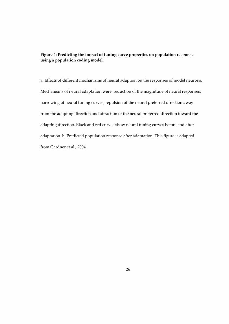
Figure 4: Predicting the impact of tuning curve properties on population response using a population coding model. 

 

a. Effects of different mechanisms of neural adaption on the responses of model neurons. 

Mechanisms of neural adaptation were: reduction of the magnitude of neural responses, 

narrowing of neural tuning curves, repulsion of the neural preferred direction away 

from the adapting direction and attraction of the neural preferred direction toward the 

adapting direction. Black and red curves show neural tuning curves before and after 

adaptation. b. Predicted population response after adaptation. This figure is adapted 

from Gardner et al., 2004. 

 

 

 

 

 

 

 

27 

 

Figure 4: Predicting the impact of tuning curve properties on population response using a population coding model. 

 

 

                                     Adapted from Gardner et al., 2004 

 

28 

 

Chapter 2: Capturing and decoding the dynamics of population responses to changes of motion direction

 

2.1 Introduction

Under natural viewing conditions, circuits in visual cortex must represent the 

information contained in a continuous stream of images that often contains abrupt 

changes in stimulus properties, such as motion direction. How are changes in the 

direction of stimulus motion represented in the dynamics of V1 population response? 

This question has been explored previously by examining the impact of neuronal tuning 

curves (Muller et al., 1999; Dragoi et al., 2000; Felsen et al., 2002; Kohn and Movshon, 

2004). However, this approach fails to provide accurate measurement of population 

response (Gardner et al., 2004).  

In this chapter, I describe experiments utilizing a new approach, voltage‐

sensitive dye imaging, to record the dynamics of population response directly. I chose 

ferrets as my experimental animal model, because it has been shown by optical imaging 

studies that direction preference is arranged in a systematic fashion in ferret V1 (Weliky 

et al., 1996), which allows me to identify the preferred directions for every pixel within 

my imaging data. By comparing the patterns of activity revealed by voltage‐sensitive 

dye imaging with the map of preferred direction I have been able to show how the brain 

responds to motion transitions.   

 

29 

 

2.2 Results

2.2.1 The dynamics of the population response to motion transition in primary visual cortex vary as a function of direction deviation angle

Voltage‐sensitive dye imaging of ferret visual cortex revealed strong and stable 

columnar activity patterns in response to random dot patterns that moved in a constant 

direction (Figure 5).  In contrast, abrupt changes in direction of motion (see Figure 6 and 

Method section for visual stimulus design) were accompanied by dynamic changes in 

the columnar patterns whose properties varied as a function of the size of the direction 

deviation.  Figure 7 illustrates for one experiment the typical transition patterns that 

were found for different direction deviation angles. In these experiments, the final 

direction of motion for each condition was identical—horizontal motion to the left—but 

was preceded by stimuli that were offset in a clockwise fashion by 45°, 90°, and 135°.  As 

expected, the columnar patterns for different offset angle conditions were significantly 

different at the start of the trial interval, but were indistinguishable at the end of the trial 

interval (Figure 7a, b and c). For a direction deviation angle of 45°, the cortical activity 

shifted smoothly from the initial pattern to the final pattern without an obvious change 

in modulation strength (Figure 7a). For a 90° direction deviation, however, the onset of 

the second stimulus was accompanied by a prominent reduction in the modulation of 

VSD signal, which was then followed by the emergence of a new stable pattern of 

activity (Figure 7b). For a direction deviation angle of 135°, there was also a noticeable 

 

30 

 

reduction in the modulation of the activation pattern during the transition period 

(Figure 7c).  

In order to understand the relation between these columnar response patterns 

and the tuning of the population response to motion direction it is necessary to convolve 

the stimulus evoked VSD maps with the direction preference map for the same region of 

cortex (Basole et al., 2003; Figure 8). The resulting population response profile (PRP) 

represents the average activity evoked by a given stimulus across all cortical sites 

expressed as a function of each site’s preferred stimulus direction (Figure 8c). The PRP 

for each stimulus condition exhibits a single major peak that, at the beginning and the 

end of the trial, corresponds to the direction of stimulus motion. In addition, there is a 

smaller minor peak consistent with the fact that tuning for stimulus direction is not 

absolute: most neurons are tuned to orientation and respond less strongly to motion in 

the anti‐preferred direction (Berman et al., 1987; Finlay et al., 1976; Moore et al., 2005). 

The PRP dynamics for a constant motion stimulus is shown in Figure 9. The peak 

direction was stabilized (Figure 9b) after the peak amplitude increased above the noise 

level (Figure 9c). The combined change in the peak direction and the magnitude of the 

population response is summarized in vector format in Figure 9d.  

 In the motion transition conditions, comparison of the PRP tuning dynamics for 

the three direction deviation angles illustrates prominent features of the population 

 

31 

 

response that differ as a function of direction deviation angle.  For small direction 

deviation angles (45°), the peak of the population response swept smoothly and 

gradually from the initial direction (135°) to the final direction (180°) taking the shortest 

route across the intermediate direction space (Figure 10a). For somewhat larger 

direction deviation angles (90°), the peak of the population response also followed the 

shortest route across the intermediate direction space (i.e. from 90°‐180°), but the 

transition process became compressed in time with a sharp jump in the peak of the 

population response that coincided with a reduction in the modulation of the VSD 

signal. For larger direction deviation angles (135°), the population response exhibited a 

distinctive triphasic pattern: an initial phase in which the peak direction turned away 

from the shortest route between the initial and final direction, a second phase in which 

the peak rapidly jumped by 180° in concert with a reduction in magnitude, and a third 

phase in which the peak direction gradually settled on the final direction. The combined 

changes in the peak direction and the magnitude of the population response for these 

three direction deviation angles are summarized in vector format in Figure 10b.   

To confirm the systematic relation between the dynamics of the peak population 

response and direction deviation angle I quantified the average population response for 

the full range of direction deviation angles in experiments from 10 animals.  The 

properties of the population dynamics varied continuously as a function of direction 

 

32 

 

deviation angle with an inflection point that is evident at direction deviation angles of 

112.5°.  For direction deviation angles of 22.5°‐90°, the peak direction during the 

transition swept across the intermediate direction space between the initial and final 

direction (Figure 11a). Within this group, the rate of transition measured at the midpoint 

of change in peak direction (°/ms) became larger as the direction deviation angle 

approached 90° (Figure 11d). For direction deviation angles greater than or equal to 

112.5°, the peak direction during the transition exhibited the “triphasic” pattern (Figure 

11a). Within this group, the rate of transition became smaller as the direction deviation 

angle approached 180° (Figure 11d). The average magnitude of the peak population 

response also varied systematically with direction deviation angle. For most direction 

deviation angles, there was a transient reduction in magnitude that reached its 

maximum at the midpoint of the change in peak direction (Figure 11b and c). This 

reduction in magnitude became greater with increasing direction deviation angle 

reaching its maximum at 112.5° and then becoming smaller with larger direction 

deviation angles (Figure 11e). For those angles where there was a prominent reduction 

in response, there was an equally prominent recovery which could exceed the 

magnitude of response to the initial direction of motion (Figure 11b and c). The 

magnitude at the end of the data acquisition period was lowest for the smallest angles in 

my sample (22.5°, 45°) and reached its highest value for the 112.5° direction deviation 

 

33 

 

angle.  For a direction deviation angle of 180° (i.e., a stimulus that reverses direction), the 

dynamics of the population response became a simple step function with a 180° jump 

during the middle of the transition process and little change in magnitude (Figure 11a 

and d).  I confirmed that the dynamics of the population response were not affected by 

the difference imaging strategy that I employed to enhance the VSD signal to noise ratio: 

analysis of the population response based on single condition images yielded similar 

results (Figure 12).  

2.2.2 The spike discharge population response constructed from unit recording data is consistent with VSDI measurements

Voltage‐sensitive dye imaging is a powerful technique for measuring the 

responses of large populations of neurons with fine temporal resolution. However, VSD 

responses are a mixture of sub‐threshold and supra‐threshold voltage signals, raising 

the possibility that the dynamics associated with changes in motion direction that I have 

described may not be evident in the spiking activity of V1 neurons. To address this 

issue, I used extracellular recordings from layer 2/3 neurons to reconstruct the dynamics 

of spiking activity that would be expected for the population response (Figure 13). I 

assume that the direction tuning function of a single neuron (i.e. the relative response of 

a single neuron to different directions of motion) can be used to infer the relative activity 

of a large population of neurons with similar tuning functions, but with different 

 

34 

 

preferred directions of motion (Treue et al., 2000).  Assuming that the direction tuning 

curve of a single neuron is representative of a large population of single neurons, the 

spike discharge PRP for a stimulus moving in a single direction will be identical to the 

direction tuning curve of single neurons whose preferred direction of motion 

corresponds to the direction of stimulus motion (Figure 13a). 

By similar reasoning, the spike discharge PRP for a stimulus that changes its 

direction of motion can be extrapolated from a single neuron’s response using a series of 

motion transition stimuli that (1) cover the full range of motion directions and (2) where 

each stimulus is composed of two successive motion stimuli with the same direction 

offset angle (see Methods).  Figure 13b illustrates the spike discharge PRP estimated 

from a single unit responding to motion transition stimuli with a direction deviation 

angle of 90°.  The pattern of activity estimated for the population response exhibits all 

the basic features that would be expected based on the VSD imaging (e.g., Figure 7b), 

notably strongly tuned responses to the first and second stimulus separated by a rapid 

transition in which there is a strong reduction in the tuned response.  The PRPs 

generated with VSD imaging reflect the average activity of large numbers of neurons 

that have somewhat different direction tuning functions (see Li et al., 2006 

Supplementary Table 1 for an analysis of the variation of single neuron direction tuning 

in ferret V1.).  In order to better approximate the neuronal population response, I 

 

35 

 

examined the response of multiple single units (N= 18) to three direction deviation 

angles (45°, 90° and 135°) and then averaged the PRPs after proper alignment based on 

each neuron’s preferred direction (Figure 14a). The dynamics of peak direction and peak 

amplitude of the average spike discharge PRP varied consistently with direction 

deviation angle, matching the characteristic features computed from the VSD data 

(Figure 14b and c).  For example, the peak of the population response accompanying a 

45° deviation advanced smoothly and slowly through the intervening directions.  In 

contrast, the peak of the population response associated with a 135° deviation exhibited 

the triphasic pattern found with VSD imaging (movement away from the intervening 

directions, a rapid 180° jump, and smooth decay to the second direction of motion).  

Difference in the magnitude of the tuned response was also consistent with the results of 

VSD imaging; i.e. small reductions in magnitude for small angular offsets and large 

reductions for larger angular offsets.   

Thus, the dynamics of peak direction and peak amplitude computed for spike 

data are consistent with those computed from the VSD data (Figure 11), demonstrating 

that the population response patterns are preserved at the spike level. 

 

36 

 

2.3 Summary

In this chapter, I used voltage‐sensitive dye imaging to explore how changes in 

the direction of stimulus motion are represented in the dynamics of V1 population 

response. I found that dynamics of the population response vary as a function of 

direction deviation angle. For direction deviation angles smaller than 90°, the peak 

direction sweeps smoothly from the initial direction to the final direction.  For direction 

deviation angles larger than 112.5°, the peak direction transiently deviates away from 

the direction of the second stimulus, then exhibits a step function that transiently 

overshoots and then settles on the final direction. Dynamics of peak amplitude also vary 

as a function of direction deviation angle. There is often a “notch” during the transition 

which is largest when the direction deviation angles are near 90°. These findings were 

confirmed by unit recording experiments. 

 

2.4 Materials and methods

All experimental procedures were approved by the Duke University Institutional 

Animal Care and Use Committee  and were performed  in  compliance with guidelines 

published by the US National Institutes of Health.  

 

37 

 

2.4.1 Animal preparation

Ferrets were anesthetized with ketamine (50 mg/kg), shaved and scrubbed. The 

femoral vein was  cannulated  for delivery of 5% dextrose  in  lactated Ringer’s  solution 

and  paralytic,  a  tracheotomy  performed,  and  the  ferret  placed  in  a  stereotaxic  head 

frame. A mixture of nitrous oxide and oxygen (2:1) with halothane or isoflurane (2‐2.5%) 

was  administered  and  adjusted  if  necessary  based  on  EKG  and  expired  CO2.  Body 

temperature was maintained at 37°C, and silicone oil was used to protect the corneas. A 

craniotomy was performed above primary visual cortex and the dura removed. 

A stainless steel chamber was cemented (Dycal, Dentsply) to the skull. Intrinsic 

imaging was performed before voltage‐sensitive dye imaging. For intrinsic imaging, the 

chamber was  filled with  ringer’s  solution  and  sealed with  a  glass  coverslip  to  allow 

viewing  of  the  cortical  surface.  For  voltage‐sensitive  dye  imaging  experiments,  the 

chamber was filled with agar (0.7%) and sealed with a glass coverslip to allow viewing 

of the cortical surface.  

After  completing  surgical  procedures,  incisions  and  pressure  points  were 

infiltrated with  bupivacaine  and  anesthesia  (halothane  or  isoflurane) was  lowered  to 

0.75‐1%.  The  animal  was  paralyzed  with  rocuronium  bromide  to  prevent  eye 

movements.  Nitrous  oxide  and  oxygen  ratio  was  reduced  to  1:1.  This  reduction  in 

 

38 

 

anesthesia was necessary to allow visual stimulation to activate cortical circuits. Expired 

CO2 level was maintained at 3.5‐4.5% throughout the experiment. 

2.4.2 Intrinsic signal optical imaging

The cortical surface was visualized through a tandem lens macroscope attached 

to  a  low‐noise  CCD  camera.  The  timing  of  stimulus  presentation  and  collection  of 

reference and stimulus frames were all controlled by software from Optical Imaging Inc 

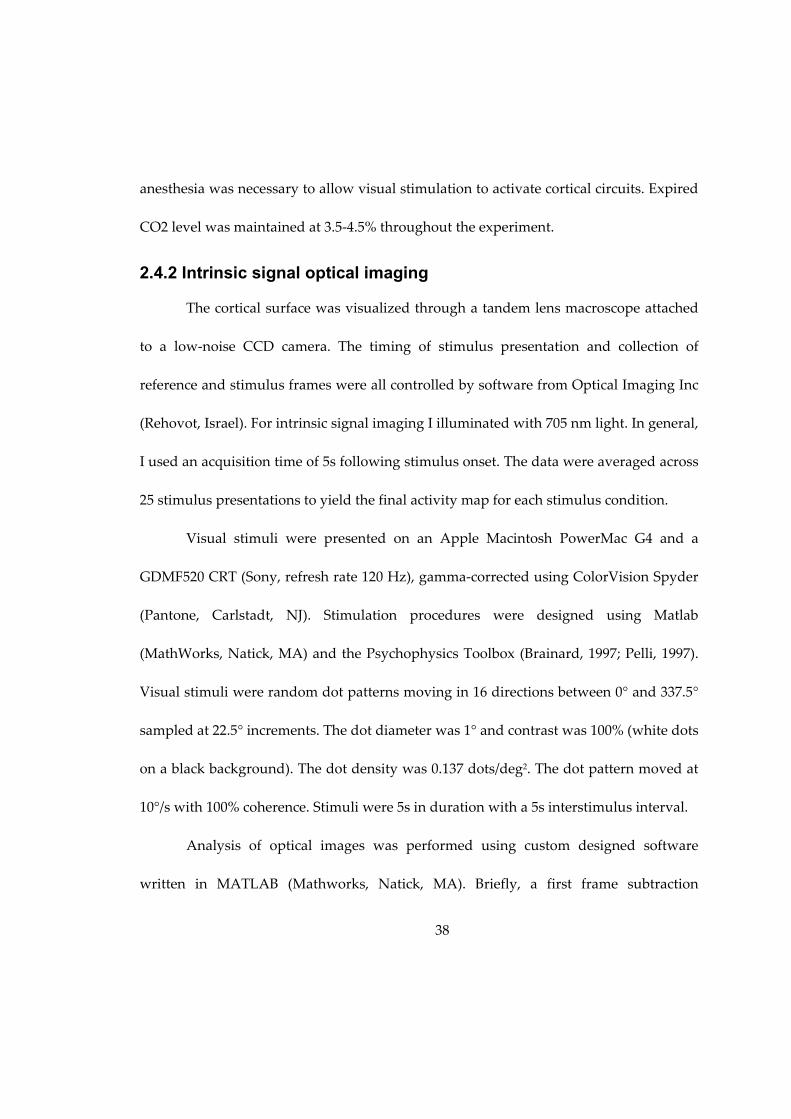
(Rehovot, Israel). For intrinsic signal imaging I illuminated with 705 nm light. In general, 

I used an acquisition time of 5s following stimulus onset. The data were averaged across 

25 stimulus presentations to yield the final activity map for each stimulus condition.  

Visual  stimuli  were  presented  on  an  Apple Macintosh  PowerMac  G4  and  a 

GDMF520 CRT (Sony, refresh rate 120 Hz), gamma‐corrected using ColorVision Spyder 

(Pantone,  Carlstadt,  NJ).  Stimulation  procedures  were  designed  using  Matlab 

(MathWorks, Natick, MA) and  the Psychophysics Toolbox (Brainard, 1997; Pelli, 1997). 

Visual stimuli were random dot patterns moving in 16 directions between 0° and 337.5° 

sampled at 22.5° increments. The dot diameter was 1° and contrast was 100% (white dots 

on a black background). The dot density was 0.137 dots/deg2. The dot pattern moved at 

10°/s with 100% coherence. Stimuli were 5s in duration with a 5s interstimulus interval.  

Analysis  of  optical  images  was  performed  using  custom  designed  software 

written  in  MATLAB  (Mathworks,  Natick,  MA).  Briefly,  a  first  frame  subtraction 

 

39 

 

(Bonhoeffer  and  Grinvald,  1996) was  performed  followed  by  a  circularly  symmetric 

spatial  filter  (pass band between  1.0‐6.7  cycles/mm,  implemented  as  a  low‐pass mean 

filter 5 pixels  in diameter,  followed by a high‐pass mean  filter 35 pixels  in diameter). 

Because most neurons  in  ferret primary visual cortex exhibit a reduced but significant 

response  to motion  in  the non‐preferred direction  (Moore et al., 2005),  the single‐pixel 

direction tuning curve was fitted to a double Gaussian function:  

M(θ | A0,A1,A2,ϕ1,ϕ2,σ ) = A0 + A1e−(θ −ϕ1 )2

2σ 2 + A2e−(θ −ϕ 2 )2

2σ 2             (1) 

Here M is the response of a pixel as a function of the direction of motionθ , A0 is 

the  untuned  response  component, A1  and A2  are  the  strength  of  the  response  to  the 

preferred  and  nonpreferred  direction,  respectively,  and  φ1  is  the  corresponding 

preferred  and  φ2  is  the  corresponding  nonpreferred  direction,  σ  is  the  tuning width. 

There  were  five  parameters  for  36  degrees  of  freedom,  because  φ1  and  φ2  were 

constrained  to  be  180°  apart  from  each  other. When  the  fitting  procedure  led  to  a 

solution  with  A2>A1,  I  exchanged  A1  and  φ1  with  A2  and  φ2  so  that  φ1  always 

corresponded  to highest peak  in  the direction  tuning curve,  i.e.  the neuron’s preferred 

direction. The direction map is obtained by plotting for each pixel its preferred direction. 

The fitting procedure is described below in the subsection on the fits for the population 

response profile (PRP).  

 

40 

 

2.4.3 Voltage-sensitive dye imaging (VSDI)

I followed the protocol for VSD imaging described by Grinvald and collaborators 

(Grinvald  and  Hildesheim,  2004;  Sharon  and  Grinvald,  2002;  Shoham  et  al.,  1999). 

Briefly,  the  cortex  was  stained  with  the  VSD  RH‐1691  by  circulating  the  dye  in  a 

chamber over the cortex for 2 hr and washing it out with ringer’s solution.  Images were 

acquired with a CCD digital camera at a frame rate of 340 Hz and a spatial resolution of 

30  μm per pixel. Frame  acquisition was  synchronized with  the heartbeat. Respiration 

was  stopped during  the  acquisition. The  cortex was  illuminated  by  a  100 W halogen 

light.  The  filter  settings  were  as  described  previously  (Shoham  et  al.,  1999):  The 

excitation  filter was band‐pass  at 630 ± 10 nm,  and  the  emission  filter was high‐pass, 

with a cutoff at 665 nm.  

In the motion transition experiments, the visual stimuli started with 150 ms gray 

screen presentation followed by a 300 ms flickering dot pattern, which was designed to 

activate  the  cortex  uniformly,  without  preference  for  any  direction  domain.  

Subsequently,  two  stimulus  components  each  lasting  1  s  were  presented,  with  the 

direction of the second component different by an angle which varied between 22.5° to 

180° with 22.5° angular increments. The parameters of the random dot pattern were the 

same  as  those  in  the  intrinsic  imaging  experiments.  The  average  luminance was  the 

same  for  the  two motion  components as well  as  for  the  flicker  stimulus. A difference 

 

41 

 

map was determined  to  obtain  a  higher  signal  to  noise  ratio, which meant  that  each 

stimulus condition was paired with another one with 90° angular offset in the direction 

of both its motion components (Figure 6).  

2.4.4 VSDI data analysis

The evoked response to each stimulus was calculated for each pixel in three steps 

in  order  to  eliminate  artifacts due  to  heartbeat  and  respiration  (Grinvald  et  al.,  1984; 

Sharon et al., 2007). First, the response was averaged across trials. Second, the response 

averaged across  the 150 ms prior  to stimulus onset was subtracted  in order  to remove 

slow  stimulus‐independent  fluctuations  in  illumination  and  background  fluorescence 

levels. Finally, ΔF/F was determined by subtracting the response to a blank stimulus and 

dividing by  it.  In addition,  the data were high‐pass  filtered  (low  frequency  cut off 1.0 

cycles/mm,  implemented  as  a  high‐pass mean  filter  35  pixels  in diameter)  to  remove 

spatial gradients and isolate the local modulation patches. 

The direction preference map acquired by intrinsic imaging was aligned with the 

images  acquired  by  VSD  imaging  using  the  blood  vessel  patterns.  To  interpret  the 

patterns of activity evoked by various stimulus configurations, I calculated a population 

response profile (PRP), which captured the relative activation of each pixel in the region 

of interest (ROI) in terms of the pixelʹs preferred direction (Basole et al., 2003; Figure 8c). 

Specifically, the pixels inside the ROI were sorted into 36 bins by the preferred direction. 

 

42 

 

The averaged values for these pixels in the patterns of activity were calculated for each 

direction bin. The  resulting histograms were  fitted with double Gaussian  functions  to 

determine the peak direction and amplitude (Figure 8d and e). 

The following functions were used to analyze the PRPs obtained from difference 

images: 

M(θ | A0,A1,A2,ϕ1,ϕ2,ψ1,ψ2,σ) = A0 + A1e−(θ −ϕ1 )2

2σ 2 + A2e−(θ −ϕ 2 )2

2σ 2 − A1e−(θ −ψ1 )2

2σ 2 − A2e−(θ −ψ2 )2

2σ 2

   (2)         

Here, M  is  the  response,  θ   is  the preferred direction of  the neurons, A0  is  the 

remaining untuned response component, A1 and A2 are the responses of pixels for which 

the  stimulus  corresponds  to  the  preferred  and  nonpreferred  directions,  respectively, 

ϕ1,ϕ2,ψ1 andψ2  are the corresponding peak directions and σ is the tuning width. In total 

there were 5 parameters for 36 degrees of freedom, because φ1 and φ2 were constrained 

to be 180° apart from each other and ψ1 and ψ2  were constrained to be 180° apart from 

each other and to be 90° apart from φ1 and φ2 , respectively.   

For  each  time  frame,  the  squared  difference  between  the  measured 

responseMexp(θ)  and  the  fitting  functionM(θ | A0,A1,A2,ϕ1,ϕ2,ψ1,ψ2,σ) was minimized 

as  a  function  of  the  parameters  by  least  squares  curve  fitting  using  Optimization 

Toolboox in Matlab (lsqcurvefit). To avoid sub‐optimal solutions corresponding to local 

minima, the fitting procedure was repeated 800 times and the solution with the  lowest 

 

43 

 

difference  was  retained.  The  average  R  square  value  of  the  fits  was  around  0.85. 

Incorporating additional parameters in the fitting function did not significantly improve 

the R square value. 

In order  to determine  the  robustness of  the estimated  fitting parameters,  I  first 

estimated  the  error  in  the  binned  PRP  using  a  bootstrap  procedure  (Davison  and 

Hinkley, 1997). The original PRP for the example data set was obtained using 48‐50 trials 

per stimulus condition. I created 10 datasets by randomly drawing, with replacement, 40 

trials  from  the  original  set,  and  determined  the  PRP  for  each  of  them.  The  standard 

deviation in the PRP across these sets was used as an estimate for the error in the PRP. It 

did  not  exceed  20%  of  the  peak  response. The  effect  of  this  variability  on  the  fitting 

procedure was  estimated by using  400 PRPs generated  by  adding  a  random noise  to 

each bin with a standard deviation as much as (20%) or larger (30%) than the estimated 

PRP variability. The fits to PRPs at steady state (prior to the motion transition and after 

the motion  transition) were not  significantly  affected. For  instance,  at  a noise  level of 

30%,  the peak direction and amplitude averaged across  the 400 sample PRPs matched 

those determined from the fit to the data to within 1%, with a standard deviation of 2.7° 

and 9% of the mean, respectively. The fits remained good during the motion transition 

for small deviations such as 45°, but when the angle of deviation was 90° the fits were 

affected by  the added noise due  to  the reduction  in  the modulation of  the VSD signal. 

 

44 

 

For instance, for the latter I obtained at 200 ms after the change of the stimulus motion, a 

standard deviation of 22° and 25% of  the mean,  for  the peak direction and amplitude, 

respectively. 

I also performed the PRP analysis on single condition maps (Figure 12);  in that 

case each PRP was fitted by Equation (1). Note that for the PRP analysis θ  corresponds 

to the preferred direction of the pixel, whereas in the original application of Equation (1) 

it  was  the  stimulus  direction.  These  two  interpretations  of  the  same  formula  are 

illustrated in Figure 12a and b. 

2.4.5 Electrophysiology

Single unit activity was recorded extracellularly from V1 with MPI 

microelectrodes (impedance = 1.0 MΩ, Microprobe Inc, Gaithersburg, MD). Action 

potentials were recorded from the supragranular layers (<600 μm) and discriminated 

using Spike2 software (Cambridge Electronic Design, Cambridge, UK). The visual 

stimulus was the same as the one used in VSDI experiments. However, the direction 

deviation angle between the two components was held constant, and the direction of the 

first stimulus was varied instead across 16 angles with 22.5° angular increments (Figure 

13b). I displayed the activation relative to the spontaneous activity, which was obtained 

by subtracting the response to a blank stimulus (population averages are shown in 

Figure 14a). The reconstructed population response profile was then fitted by Equation 

 

45 

 

(1) to identify the peak direction and amplitude (Figure 14b and c). In order to be 

consistent with the VSD experiments, only the modulated component is shown (the 

untuned component has been removed).

 

46 

 

 

Figure 5: The population response to a constant motion stimulus in ferret primary visual cortex. 

VSD images acquired using a visual stimulus with a constant motion direction (135°). 

The signal strength becomes stronger over time while the activity pattern remains the 

same. Each frame of image is the averaged response of 50 msec. 

 

 

 

47 

 

 

 

Figure 5: The population response to a constant motion stimulus in ferret primary visual cortex. 

 

 

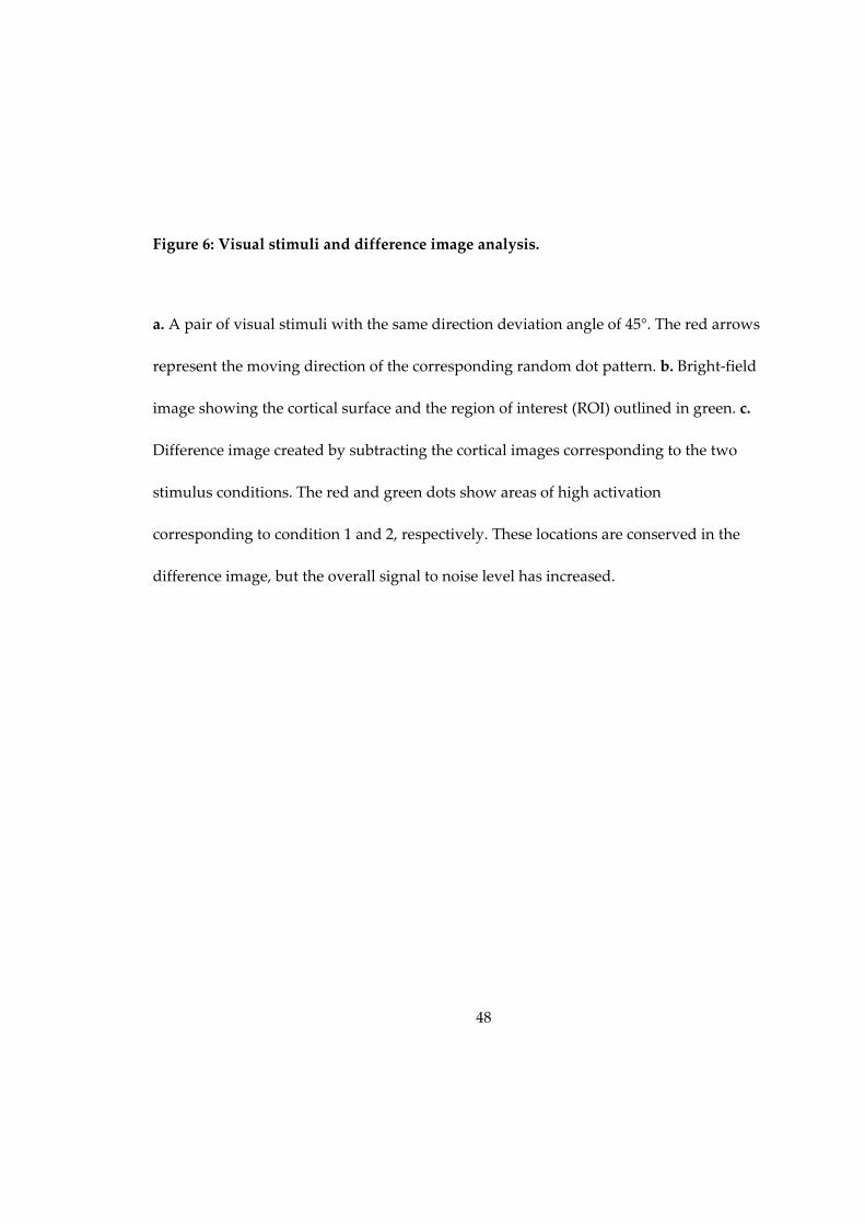
48 

 

 

Figure 6: Visual stimuli and difference image analysis. 

 

a. A pair of visual stimuli with the same direction deviation angle of 45°. The red arrows 

represent the moving direction of the corresponding random dot pattern. b. Bright‐field 

image showing the cortical surface and the region of interest (ROI) outlined in green. c. 

Difference image created by subtracting the cortical images corresponding to the two 

stimulus conditions. The red and green dots show areas of high activation 

corresponding to condition 1 and 2, respectively. These locations are conserved in the 

difference image, but the overall signal to noise level has increased. 

 

49 

 

Figure 6: Visual stimuli and difference image analysis. 

 

 

 

50 

 

 

Figure 7: The population response to motion transitions with different direction deviation angles in ferret primary visual cortex. 

 

a. VSD images acquired during a 45° deviation in motion direction. The activity pattern 

shifts smoothly from one stable pattern to the next without a decrease in signal strength. 

b. VSD images acquired during a 90° deviation in motion direction. During the 

transition the activity pattern decreases in magnitude. c. VSD images acquired during a 

135° deviation in motion direction. The magnitude of the activity pattern also decreases 

during the transition.  

 

 

 

 

 

 

 

 

 

 

 

51 

 

 

Figure 7: The population response to motion transitions with different direction deviation angles in ferret primary visual cortex. 

 

 

52 

 

 

Figure 8: Population response profile (PRP) analysis and decoding method for the peak direction and amplitude. 

 

a. A single time‐frame of the VSD difference image. b. The direction preference map 

acquired using intrinsic imaging. c. PRP analysis quantifies the mean stimulus‐evoked 

activation of pixels with a given preferred direction. Each component in the difference 

image leads to a major and a minor peak and trough, respectively, each of which can be 

fitted by a Gaussian. d. Fit of the PRP to a combination of two upward and two 

downward Gaussian functions as given in Eq.2 in methods. e. The peak direction and 

amplitude is determined from the fitting function as the location and height of the 

highest peak. 

 

53 

 

Figure 8: Population response profile (PRP) analysis and decoding method for the peak direction and amplitude. 

 

54 

 

 

Figure 9: Dynamics of the population response to a constant motion stimulus in ferret primary visual cortex.   

 

a. Population response profile analysis. Vertical dashed lines represent the time at which 

the motion stimulus was on. b. Dynamics of peak direction. c. Dynamics of peak 

amplitude. d. Dynamics of direction vector.   

 

 

 

 

 

55 

 

 

Figure 9: Dynamics of the population response to a constant motion stimulus in ferret primary visual cortex.   

 

 

56 

 

 

Figure 10: Dynamics of the population response to motion transition in ferret primary visual cortex vary as a function of direction deviation angle.   

 

a. Population response profile analysis for direction deviation angles of 45°, 90° and 

135°. Vertical dashed lines represent the time at which the motion direction changed. 

Grey dots represent the decoded peak directions. b. Dynamics of direction vectors. Grey 

arrows show the direction of time flow. 

 

57 

 

 

Figure 10: Dynamics of the population response to motion transition in ferret primary visual cortex vary as a function of direction deviation angle.   

 

58 

 

 

Figure 11: Dynamics of the population direction tuning function depend on direction deviation angle.   

 

a. Dynamics of normalized peak direction for different direction deviation angles, as 

labeled in the graph (n = 3 animals for direction deviation angles of 22.5°, 45°, 67.5°, 90°, 

112.5°, 135° and 157.5°; n = 2 animals for direction deviation angle of 180°). b‐c. 

Dynamics of normalized peak amplitude for direction deviation angles < 90° and angles 

> 112.5°, respectively. d. Rate of transition (°/ms) near the midpoint of change in peak 

direction (results are mean ± s.e.m.). e‐f. Normalized peak amplitude near the midpoint 

of change in peak direction and at the final steady state, respectively (results are mean ± 

s.e.m.).  

 

 

 

 

 

 

 

 

59 

 

 

 

Figure 11: Dynamics of the population direction tuning function depend on direction deviation angle.   

 

60 

 

 

Figure 12: Results obtained using PRP analysis on single condition images are similar to that obtained from difference images.   

 

a. PRP analysis for direction deviation angles 45°, 90° and 135°, as labeled in the graph. 

Vertical dashed lines represent the time at which the motion direction changed. Grey 

dots represent the peak directions. b‐e. Dynamics of peak direction, normalized peak 

direction, peak amplitude and normalized peak amplitude, respectively. 

 

61 

 

 

Figure 12: Results obtained using PRP analysis on single condition images are similar to that obtained from difference images.   

 

 

62 

 

Figure 13: Dynamics of the population response to changes of motion direction can be extrapolated from unit recording experiments. 

 

a. The spike discharge PRP for a stimulus moving in a single direction could be inferred 

from direction tuning curve of single neurons. b. Population response profile for motion 

transition is computed by varying the direction of the first movement component 

between 0° and 360°, while maintaining a constant direction deviation with the second 

component. An example spike discharge PRP so constructed for a direction deviation 

angle of 90° is shown here.  

 

 

 

 

 

 

 

 

 

 

 

 

63 

 

Figure 13: Dynamics of the population response to changes of motion direction can be extrapolated from unit recording experiments. 

 

 

 

64 

 

Figure 14: The population response constructed from electrophysiological data is consistent with VSDI measurements. 

 

a. Average of constructed PRPs for, from left to right, a direction deviation angle of 45° 

(n = 7 sites), 90° (n = 7 sites) and 135° (n = 4 sites). b‐c. The corresponding dynamics of 

normalized peak direction and amplitude for direction deviation angles 45°, 90° and 

135° (results are mean ± s.e.m.). 

 

65 

 

 

Figure 14: The population response constructed from electrophysiological data is consistent with VSDI measurements. 

 

 

 

 

 

 

 

66 

 

Chapter 3: Mechanism of population response to changes in motion direction: linearity vs non-linearity

 

3.1 Introduction

  The experiments described in Chapter Two have shown that the dynamics of the 

population response to motion transitions in primary visual cortex vary as a function of 

direction deviation angle. What are the mechanisms that underlie the dynamics? Many 

previous studies have shown changes in tuning curves after orientation adaptation or 

direction adaptation, suggesting that the population response to stimulus transitions 

involves significant non‐linearities (Muller et al., 1999; Dragoi et al., 2000; Felsen et al., 

2002; Kohn and Movshon, 2004). However, the dynamics of population response might 

also be explained by the linear summation of the cortical response elicited by the two 

stimulus components.  Ben‐Yishai et al. investigated the process of stimulus transition 

using computational modeling approaches. They found the population response in V1 

during the stimulus transition could follow a static wave pattern (linear) or a travelling 

wave pattern (nonlinear) depending on the properties of feed forward inputs and 

recurrent connections (Ben‐Yishai et al., 1995).  If the recurrent connections are non‐

orientation selective and the LGN inputs are highly orientation selective, the brain 

activation follows static wave pattern during the orientation transition. During the 

 

67 

 

transition, the activity profile that peaks at the initial orientation decays in magnitude 

while another activity profile peaks at the new orientation grows. In contrast, if the 

recurrent connections are highly orientation selective and the LGN inputs are non‐

orientation selective, the brain activation follows a traveling wave pattern. During the 

transition, the population activity travels across the intermediate orientation space 

without significant change in its shape.  

In this chapter, I construct a simple linear combination model and compare the 

predicted dynamics of the population response to those that are observed in Chapter 

two. I also conduct voltage‐sensitive dye imaging experiments that allow me to compare 

the response to the motion transition with that expected from the linear sum of the 

response to the component directions of motion. 

3.2 Results

3.2.1 A linear combination model explains certain aspects of the population response to rapid changes in motion direction

What accounts for these systematic departures of the population response from 

the trajectory of the moving stimulus? At least some of these effects might be explained 

by a simple linear summation of the gradual reduction in response to the first direction 

of motion combined with the gradual increase in response to the second direction of 

motion. Smooth shifts in the peak of the population response with little decline in 

 

68 

 

magnitude might be expected when the populations of neurons most activated by the 

two individual stimuli (‘the major peaks’) are partially overlapping. Significant 

reductions in magnitude accompanied by abrupt jumps in the population peak would 

be expected when the major peaks for the two stimuli are largely complementary (~90° 

offset), and the triphasic transition pattern might result when the angular offsets are so 

great that the major peak associated with the first stimulus partially overlaps the minor 

peak of the second stimulus. To test this possibility, I have constructed a simple linear 

combination model in which the cortical response to motion transition was modeled as a 

weighted sum of responses to the components (Figure 15a). The PRPs of two motion 

components were obtained from a fit to the VSD data shown in Fig.1 (Figure 15b), while 

the dynamics of the weighting factors were assumed to be simple linear processes 

(Figure 15c). The dynamics of population response to motion transitions with different 

direction deviation angles predicted by the model were shown in Figure 16a‐d. I found 

that the linear combination model was sufficient to account qualitatively for many of the 

features associated with the dynamics of the population response during the transition. 

For example, the linear model predicts the smooth progression through intermediate 

directions for small direction deviations and the triphasic pattern for larger direction 

deviation angles. It also accounts for the systematic relation between direction deviation 

angle and the transient reduction in response during the transition. I performed a 

 

69 

 

sensitivity test for two parameters in the model: direction selectivity and tuning width. 

Enhancement of direction selectivity or increase of tuning width will shift the dynamics 

of peak direction towards the smooth progression (S Shape) mode while away from the 

triphasic pattern mode (Figure 17). 

Note, however, that the linear summation model failed to account for the 

changes in magnitude that follow the motion transition (Figure 11f). The magnitude at 

the end of the data acquisition period was lowest for the smallest angles in my sample 

(22.5°, 45°) and reached its highest value for the 112.5° direction deviation angle. These 

changes are likely to reflect longer lasting adaptation mechanisms that have been the 

subject of numerous previous studies (Dragoi et al., 2002; Vautin et al., 1977; Priebe and 

Lisberger, 2002; Carandini et al., 1998).  

In my linear model, I assumed that the onset response latency for the second 

motion component was the same as the offset response latency for the first motion 

component. Some studies showed that the onset latency is longer than offset latency 

(Bair et al., 2002). Modification of the weighting factor dynamics based on these studies 

does not impact the overall pattern of the model predictions. In fact, the key features 

that appear to account for these population effects are: (1) the non‐instantaneous nature 

of circuit dynamics, (2) the presence of single neuron responses to both the preferred 

 

70 

 

and anti‐preferred directions of motion, and (3) the broad tuning of individual neurons 

for motion around the preferred and anti‐preferred directions.    

3.2.2 Additional nonlinear mechanisms shape the dynamics of population response

In the previous section, I have shown that a simple linear combination model 

could explain many features associated with the dynamics of the population response 

during the transition. However, one might argue that the inputs (Fig. 4b and c) that were 

fed into the model do not necessarily represent biological conditions. To address this 

concern, I have conducted VSDI experiments that captured the cortical responses to 

motion transitions and the corresponding individual motion components. These 

experiments allowed me to directly compare the response to the change in motion 

direction with that expected from the linear sum of the response to the component 

direction of motion (Figure 18).  For large deviation angles (135°) the linear sum of the 

components is a close match for the peak direction and peak amplitude time course.  But 

for smaller deviation angles, the linear sum differed from the transition condition, 

especially in the magnitude of the response during the transition: the linear sum 

condition exhibits a prominent reduction in response magnitude that was not evident in 

the experimental condition (Figure 19a). Linear regression analysis of the linear 

summation and experimental conditions from 3 experiments (Figure 20) confirmed that 

 

71 

 

the linear summation of the component responses accurately predicted the dynamics of 

population response in the experimental conditions prior to the transition (correlation 

coefficient equals to 0.97 ± 0.01, 0.99 ± 0.01 and 1.00 ± 0.01 for 45°, 90° and 135° 

respectively), and for values taken during the motion transition (100 ms to 300 ms) for 

the 135° direction deviation angle, but not for the 45° and 90° conditions (correlation 

coefficient equals to 1.97 ± 0.05, 1.26 ± 0.03 and 0.98 ± 0.02 for 45°, 90° and 135° 

respectively). As shown by the vector plots (Figure 19b), the transition between the 

initial state and final state in the experimental conditions is smoother compared to the 

linear summation conditions for the smaller direction deviation angles (45° and 90°). 

Thus, while the basic qualities of the population response to motion transitions are 

consistent with linear summation, additional nonlinear mechanisms shape the dynamics 

of population response both during and after motion transitions.    

3.3 Summary

In this chapter, I showed that a linear combination model could explain many 

aspects of the population response to motion transitions, such as the S‐shape pattern and 

triphasic pattern for the dynamics of peak direction and the reduction of peak amplitude 

in the middle of motion transition. However, additional nonlinear mechanisms also 

involved to shape the dynamics of population response. For example, the response 

amplitude after motion transition is modulated in a systematical fashion that is 

 

72 

 

consistent with previous adaptation studies. The magnitude of tuning strength for small 

motion transition, such as 45°, is larger compared to the linear sum condition, which 

makes the transition process even smoother than what is predicted by linear 

combination model. 

 

3.4 Materials and methods

3.4.1 Linear combination model

The dynamics  of  cortical  activation was  studied  by determining  the  PRP  as  a 

function of timeM exp (θ, t) . To evaluate to what extent the cortical response to a motion 

transition  could  be  understood  in  terms  of  a  linear  combination  of  responses  to 

component stimuli, it was compared to the following linear combination model (Figure 

15a): 

Mlin(θ,t) =α(t)N1(θ)+ β(t)N2(θ)                       (3) 

Here, Mlin  is  the model  response  to  the motion  transition,  θ   is  the  preferred 

direction of the neurons, and t is time. N1 and N2 is the steady state PRP corresponding 

to  the  direction  of  the  first  and  second  component,  respectively.  α  and  β  are  the 

weighting factors for the two motion components. The functions N1 and N2 were given 

by the functional form of Equation (2), which was interpreted as the population activity 

for the stimulus direction in each of two component stimuli (Figure 15b). The parameter 

 

73 

 

values (A0 = 0.039, A1 = 0.698, A2 = 0.441 and σ = 38.3) were obtained from a fit to a typical 

VSDI dataset and φ1 was set  to  the direction of  the  first and second component  for N1 

and N2, respectively. For the first 50 ms after the motion transition, α(t) = 1 and β(t) = 0, 

whereas during the 500 ms long transition period α(t) linearly decayed to zero and  β(t) 

linearly increased to one (Figure 15c). After reaching these values α(t) and β(t) remained 

constant. To determine  the population dynamics,  I  fitted  for each  t value,  Mlin(θ,t)   to 

Equation  (2). This yielded  the peak direction  (φ1) and amplitude  (A1) as a  function of 

time (Figure 16).  

3.4.2 VSDI experiment to test the linearity

The visual stimuli used in the motion transition condition were similar to those 

described in Chapter Three. Briefly, the visual stimuli started with a 150 ms gray screen 

presentation  followed by a 300 ms  flickering dot pattern.   Subsequently,  two stimulus 

components were presented with the direction of the second component different by an 

angle of 45°, 90° and 135°. The duration of the first motion component was reduced to 

500 ms  in order  to shorten  the  imaging  time, while  the duration of  the second motion 

component was kept as 1 s.  The parameters of the random dot pattern were the same as 

those given in Chapter Three. To test for linearity, the response was also obtained to two 

control conditions for which either the first or second motion component was replaced 

by a flickering dot pattern, respectively.  

 

74 

 

Figure 15: A linear combination model explains certain aspects of the population response to motion transition. 

 

a. The response to a transition is modelled as a weighted sum of responses to the 

components.  b. Example steady state PRP for two motion components with a direction 

deviation angle of 90° obtained from a fit to the VSD data shown in Figure 1.  c. 

Dynamics of the weighting factors for two motion components with a direction 

deviation angle of 90°. The (red) weight α  of the first component decays linearly from a 

value of 1 before the transition to 0 during a 500 ms interval, whereas the (green) weight 

β   of the second component increases from 0 to 1 during that time interval.  

 

75 

 

 

Figure 15: A linear combination model explains certain aspects of the population response to motion transition. 

 

 

76 

 

Figure 16: Dynamics of population response predicted by the linear combination model. 

 

a. The resulting model PRPs are shown for direction deviation angles 45°, 90° and 135°, 

as labeled. b. Dynamics of normalized peak direction for different direction deviation 

angles, as labeled in the graph, obtained from a linear combination model. c‐d. 

Dynamics of the normalized peak amplitude for direction deviation angles < 90° and 

angles > 112.5°, respectively, obtained from a linear combination model. 

 

77 

 

 

Figure 16: Dynamics of population response predicted by the linear combination model. 

 

 

 

 

 

  

 

78 

 

 

Figure 17: Sensitivity test for two parameters in the linear combination model. 

 

a. Relationship between direction selectivity and break point. The break point is defined 

as the direction deviation angle upon which the dynamic of peak direction shifts from S‐

shape pattern to triphasic pattern. Enhancement of direction selectivity (decrease 

minor/major peak amplitude ratio) predicts a larger break point. The parameter of 

neuronal tuning width, Sigma, is set to be 38.3° in this panel.  Grey triangle indicates the 

parameters used in the model shown in Figure 15 and Figure 16 (minor/major peak 

amplitude ratio = 0.632, Sigma = 38.3°). b. Relationship between tuning width and break 

point. Broader tuning width predicts a larger break point. The minor/major peak 

amplitude ratio is set to be 0.632 in this panel. 

 

79 

 

 

Figure 17: Sensitivity test for two parameters in the linear combination model. 

 

 

80 

 

   

Figure 18: A direct test for linearity of the population response. 

 

a. Responses to motion transition with direction deviation angles of 45°, 90° and 135°. b. 

The predicted responses based on linear superposition of the transition from stimulus 

component 1 to flickering dot pattern and that from flickering dot pattern to stimulus 

component 2. c. The difference between the two.  Grey dots represent the decoded peak 

directions. 

 

 

 

 

 

 

 

 

 

 

 

 

81 

 

Figure 18: A direct test for linearity of the population response. 

 

 

82 

 

 

Figure 19: Population responses demonstrate a nonlinearity that depends on direction deviation angles. 

 

a. The corresponding dynamics of peak direction and amplitude for (red) transition 

conditions and (blue) linear sum conditions. b. Dynamics of direction vectors for 

transition conditions and linear sum conditions. Grey arrows show the direction of time 

flow. 

 

 

 

 

 

 

 

 

 

 

 

 

 

83 

 

 

Figure 19: Population responses demonstrate a nonlinearity that depends on direction deviation angles. 

 

 

 

84 

 

 

Figure 20: Evidence for nonlinear dynamics during the transition period. 

 

I show scatter plots of the PRP for the transition condition versus the sum of PRPs 

corresponding to the motion component 1 to flickering dot pattern and the flickering dot 

pattern to motion component 2 conditions. I show data from before the transition (‐200 

ms to 0 ms) in blue and during the transition (100 ms to 300 ms) in red for direction 

deviation angles 45°, 90° and 135°, as labeled. The linear summation of the component 

responses accurately predicted the dynamics of population response in the experimental 

conditions prior to the transition (correlation coefficient equals to 0.97 ± 0.01, 0.99 ± 0.01 

and 1.00 ± 0.01 for 45°, 90° and 135° respectively), and for values taken during the 

motion transition (100 ms to 300 ms) for the 135° offset condition, but not for the 45° and 

90° offsets (correlation coefficient equals to 1.97 ± 0.05, 1.26 ± 0.03 and 0.98 ± 0.02 for 45°, 

90° and 135° respectively).

 

85 

 

 

Figure 20: Evidence for nonlinear dynamics during the transition period. 

 

 

 

 

 

 

 

 

86 

 

Chapter 4: Perceptual distortions in motion trajectory  

4.1 Introduction

The question of how prevailing motion stimulus conditions impact perception to 

a new motion stimulus has been studied within the realm of direction adaptation. 

Prolonged adaptation to direction stimulus has been shown to cause a direction 

aftereffect (DAE) (Levinson and Sekuler, 1976; Patterson and Becker, 1996; Phinney, 

1997; Schrater and Simoncelli, 1998; Clifford, 2002). For angles up to around 100 degrees 

between the directions of motion of the adapting and test patterns, the perceived 

direction of the test pattern tends to be repelled away from the adapting direction. For 

angles larger than 100 degrees between adapting and test directions, the perceived 

direction of the test tends to be attracted towards that of the adapter (Schrater and 

Simoncelli, 1998; Clifford, 2002). However, there are two major differences between the 

stimuli used in the typical DAE experiments and natural visual stimuli. First, the 

adapting stimuli in DAE experiments usually lasts for a long time, often for 1 min or 

longer. Such prolonged adaptation rarely happens under natural viewing conditions. 

Second, there are often intervals between the adapting stimuli and testing stimuli, which 

are absent in natural environment. Thus, the DAE effects reflect the perception of test 

 

87 

 

stimuli on steady state responses rather than the perception of a stimulus that changes 

its direction of motion per se.  

In Chapter Two, I showed that dynamics of the population response to motion 

transition vary as a function of direction deviation angle. How do these dynamics of 

population response impact motion perception? I address this question in this chapter. I 

first predict the distortions of perceived motion trajectories based on the dynamics of 

population response and then verify my predictions by conducting psychophysical 

experiments.  

4.2 Results

4.2.1 Distortions in perceived motion trajectory accord with the dynamics of the population response

Given the evidence that the neural representation of motion direction departs 

from the actual direction of stimulus motion, I asked what impact this departure might 

have on the perceived trajectory of objects that change their direction of motion.  I 

estimated the perceived trajectories for bilinear motion transitions with different 

deviation angles by assuming (1) the perceived motion direction at any given time point 

is determined by the dynamic of peak direction obtained from the population response 

(2) the moving distance within a time frame is a constant (i.e., constant speed is 

assumed) (Figure 21). For direction deviation angles less than 90° (22.5°, 45° and 67.5°), 

the perceived motion trajectories predicted by the model were more gradual (smoother) 

 

88 

 

than the actual stimulus trajectories; the degree of smoothing was greatest for the 22.5° 

stimulus and least for the 67.5° stimulus. In contrast, for direction deviation angles of 

112.5° and 135°, the perceived motion trajectories predicted by the model were more 

acute (sharper) than the actual stimulus trajectories. No perceptional distortions were 

predicted for direction deviation angles of 157.5° and 180° (Figure 22).  

These predictions were tested in a human psychophysical experiment that 

measured the perceived trajectory of a moving dot stimulus. The first phase of the dot 

motion was always along a straight line, followed by a second phase in which the dot 

assumed one of 9 different trajectories: either a straight line or a curved path on either 

side of the straight line (Figure 23). The curved trajectories could be convex (i.e., 

smoother than the line) or concave (sharper than the line). Subjects indicated the 

perceived trajectory of the second phase of dot motion by choosing between two 

alternatives: motion trajectories smoother than the line or motion trajectories sharper 

than the line. Instead of a random dots pattern, a single dot motion was chosen as the 

visual stimulus because it provided the best comparison to the results with the ferrets; it 

was critical for the humans to maintain fixation and this was nontrivially easier for a 

single dot motion display compared to a full motion display. I set the transition point 

from the first to the second motion component to be 4.9° below and 1° to the right of a 

 

89 

 

central fixation point so that the change of motion direction happened at the peripheral 

visual region (5° eccentricity). 

The psychometric functions for small direction deviation angles, such as 22.5°, 

45° and 67.5°, were shifted leftwards systematically (Figure 24a) as indicated by negative 

RC50 values (Figure 25a and b), hence the subjects’ perception of the motion trajectories 

was smoother than the actual stimulus trajectories. In contrast, the psychometric 

functions for direction deviation angles of 112.5° and 135° were shifted rightwards 

(Figure 24b) with positive RC50 values (Figure 25a and b), indicating that the subjects’ 

perception of the motion trajectories was sharper than the actual stimulus trajectories. 

These observations were further confirmed by examining the subjects’ reports for the 

bilinear stimulus trajectories. The probability of reporting smoothing trajectory was 

significantly larger than chance level (50%) for direction deviation angles at  22.5°, 45° 

and 67.5°, and significantly smaller than chance (50%) for direction deviation angles at  

112.5°, 135° (Figure 25c and d).  

4.2.2 The perception distortion for motion trajectory could not be explained by positional information

Interestingly, the distortions of motion transition perception depend on 

eccentricity. The bias gets significantly weaker in fovea visual region (Figure 26a). I 

hypothesize this effect is related to the position acuity. Ultimately, both positional 

 

90 

 

information and directional information must be integrated in judgements of motion 

trajectory. In the foveal visual region, the position acuity is so high that it provides 

perceived trajectories with high fidelity thus precludes any distortions predicted by the 

direction perception. In contrast, when eccentricity increases, the position acuity gets 

worse (Figure 26b and c) and thus the distortion of direction perception becomes more 

evident.  

Stimulus motion has been shown to impact human perception of position 

(Whitney & Cavanagh, 2000; Whitney, 2002). For example, the initial (Frohlich, 1929) or 

final position (Freyd & Finke, 1987) of a moving object can appear shifted in the 

direction of motion. Could the distortions in perceived trajectory shown in the periphery 

visual region be explained by position perception, even under a low visual acuity? To 

address this question, I have designed an experiment to reconstruct the motion 

trajectory solely based on position information (Figure 27).  My experimental results 

demonstrated that the reconstructed motion trajectory based on position information 

showed no systematic curvature bias. Therefore, position cue information did not 

contribute to the distortion of the perceived trajectory measured in my experiments. 

 

91 

 

4.3 Summary

In this chapter, I implemented a simple model to predict perception of motion 

trajectory based on dynamics of population response to motion transition. For direction 

deviation angles less than 90° (22.5°, 45° and 67.5°), the perceived motion trajectories 

were predicted to be more gradual (smoother) than the actual stimulus trajectories. In 

contrast, for direction deviation angles of 112.5° and 135°, the perceived motion 

trajectories were predicted to be more acute (sharper) than the actual stimulus 

trajectories. No perceptional distortions were predicted for direction deviation angles of 

157.5° and 180°. These predictions were verified by psychophysical experiments. I also 

demonstrated the perceptual distortion for motion trajectory could not be explained by 

position perception. 

4.4 Materials and methods

4.4.1 Experiment 1: Measure the distortion of motion transition perception.

Subjects. Subjects were four students (3 male and 1 female; average age was 27.8 years; 

standard deviation was 2.5 years) at Duke University, all with normal or corrected‐to‐

normal vision. One subject was the first author (WW) and the remaining three subjects 

were  naïve  observers.  All  experimental  procedures  were  approved  by  the  Duke 

University Institutional Review Board. 

 

92 

 

 

Apparatus.  Visual  stimuli were  presented  on  a  PowerMac  G4  and  a  GDMF520  CRT 

(Sony,  refresh  rate  120  Hz),  gamma‐corrected  using  ColorVision  Spyder  (Pantone, 

Carlstadt,  NJ).  Stimulation  procedures  were  designed  using  Matlab  (MathWorks, 

Natick,  MA)  and  the  Psychophysics  Toolbox  (Brainard,  1997;  Pelli,  1997).  The 

experiments were conducted in a dimly lit room. The subjects were seated 100 cm from 

the monitor, although they were permitted slight movement. 

 

Stimuli. The visual stimulus was a white dot (0.1° diameter, 100% contrast) presented on 

a black background. The dot moved at 10°/s in two distinct motion components. In the 

first motion component, the dot moved from left to right along a straight line for 0.3s. In 

the second motion component,  the dot moved  towards a new direction along either a 

straight line or along a curve slightly bent on either side of an imaginary straight line for 

0.3s. The transition from the first to the second motion component occurred 4.9° below 

and  1°  to  the  right  of  a  central  fixation point  so  that  the  change  of motion direction 

happened  at  the  peripheral  visual  region  (5°  eccentricity).  There  were  8  different 

direction  deviation  angles  in  the  experiment,  ranging  from  22.5°  to  180° with  22.5° 

angular  increments.  I also varied  stimuli eccentricity  systematically  (1°, 5° and 10°)  in 

order to test the relationship between eccentricity and the distortion of motion transition 

 

93 

 

perception. The direction deviation  angle was  set  to be 45°  in  these  experiments. The 

stimulus differences between this psychophysics component (a single dot on a uniform 

background) and the physiology component (a random dot pattern) were introduced for 

several  reasons,  with  the  most  critical  being  practical  –  whereas  the  ferrets  were 

anesthetized and paralyzed, the human were awake and free to make eye movements. 

Pilot studies determined that subjects were better able to maintain fixation with a single 

moving dot than with a full fields of motion.  

 

Procedure.  The  experimental  task  followed  a  two‐alternative  forced  choice  (TAFC) 

paradigm  (Green and Swets, 1966). Observers maintained  fixation on  the central point 

and observed the presentation of a moving dot, after which they indicated the perceived 

dot  motion  trajectory  by  choosing  between  two  alternatives:  a  motion  trajectory 

smoother than a bilinear line and a motion trajectory sharper than a bilinear line. To test 

how  the  perceived  motion  deviated  from  the  veridical  straight  line  trajectory  (for 

instance,  making  an  angle  of  45°  with  the  horizontal),  I  constructed  comparison 

trajectories characterized  in  terms of  the parameter RC  (relative curvature, Figure 23). 

For RC=0,  the  trajectory  is  a  straight  line;  for RC<0,  it  is  convex, with  a  direction  of 

motion just after the transition larger than 45°; for RC>0, it is concave and the direction 

of  motion  just  after  the  transition  is  less  than  45°.  The  trajectory  is  described  by 

 

94 

 

(x(t),y(t))  (t  is  time),  which  can  be  characterized  by  two  differential  equations:  

dxdt

= vx (t) and dydt

= vy (t), where vx and vy denote  the velocity components of  the dot. 

This can be simplified by eliminating time t in favor of x, yieldingdydx

=vy (x)vx (x)

. For RC>0, 

the  following  choice  leads  to  curves  satisfying my  requirements: RCyxdxyd /)ˆ(100ˆ

−= , 

where RC is a parameter and the reason for the hat on y is given below. This leads to a 

trajectory  (x,y)  that  goes  from  (0,0)  to  ))1(ˆ,1( y . When  I  define )1(ˆ/)(ˆ)( yxyxy = ,  the 

trajectory ends at (1, 1) as desired.  The explicit form is then as follows: 

)/100exp(100)/100exp(100)(

RCRCRCRCxRCxRCxy

−++−−++−

= .  

For RC<0, I exchanged the y and x coordinates to obtain: 

x(y) = RC +100y − RC exp(100y /RC)RC +100 − RC exp(100 /RC)

 

Subjects received 10 minutes of training before the data collection for each block. During 

the  training,  I  set  the RC value  to be  ‐20,  ‐10, 10 and 20. These parameters generated 

obvious  smoothing  trajectory  and  sharpening  trajectory,  allowing  the  subjects  to 

understand  the  experimental  paradigm.  Feedback was  provided  by  the  experimenter 

during  the  training  period  if  necessary  or  if  questions were  raised. During  the  data 

collection,  9  curvatures  were  assigned  for  the  trajectories  of  the  second  motion 

 

95 

 

component in each block (1 straight line and 4 curvatures on either side, RC value was 

set to be ‐8,‐6,‐4,‐2,0, 2,4,6,8). The subjects were asked to judge the trajectory solely based 

on  their perception. No  feedback was given during  the data  collection. The  task was 

presented in multiple blocks (8 different direction deviations, ranging from 22.5° to 180° 

with  22.5°  angular  increments).  To minimize  subject  bias,  I  randomized  the  number 

(from  40  to  60)  and  sequence  of  different  RC  presentation  in  each  block.  To  reduce 

chances  of  fatigue,  rest  periods were  included within  each  block  and  only  a  limited 

numbers of blocks were performed on a given day.  

 

Data  analysis.  The  psychometric  functions  relating  the  probability  P  to  the 

convexity/concavity parameter RC were fitted to a Boltzmann sigmoidal function using 

Origin (OriginLab, Northampton, MA): 

))/)exp((1/(11)( 50 RCRCRCRCP σ−+−=        (4) 

Here, the parameters are the RC value for which the probability is 50%, RC50, and 

the steepness σRC . Student t test was used to determine the significance level (* p<0.05, ** 

p<0.01, *** p<0.001). 

4.4.2 Experiment 2: Measure the noise of position judgment at different eccentricities and reconstruct motion trajectory using positional information.

Subjects. Same as Experiment 1. 

 

96 

 

Apparatus. Same as Experiment 1. 

 

Stimuli. The visual stimuli were  identical  to Experiment 1 except where noted here.  In 

this  experiment,  the  dot moved  rightwards  along  a  straight  line  for  0.3  s  and  then 

changed  its  direction  of motion  for  45°  or  135°. After  the motion  transition,  the  dot 

traveled a certain distance and disappeared. For each direction deviation angle, the dot 

could disappear  from  five different positions  (the position was  randomly chosen each 

trial and they are depicted by the colored dots in Figure 27a). The eccentricity was tested 

at 1°, 5° and 10°. 

 

Procedure.  Observers  maintained  fixation  on  the  central  point  and  observed  the 

presentation of a moving dot, after which they were asked to indicate the position where 

the dot disappeared by clicking on the position with a computer mouse. Subjects were 

allowed  to  break  the  fixation while  clicking  the mouse  in  order  to minimize motion 

errors. To prevent the subject from memorizing the positions, I jittered the starting point 

of the moving dot and aligned the data by the starting point for each trial. Subjects were 

informed  that  the positions where  the dot disappeared were  randomized, so  that  they 

would need  to make  their mouseclick  solely based on  their perception  in  the  current 

trial. Subjects received 2 minutes of training before data collection and no feedback was 

 

97 

 

given during the training. There were 600 trials and for the whole task, the direction of 

the  deviation  angle  (45°  or  135°)  and  the  position where  the  dot  disappeared were 

randomly determined. The task was broken into 5 blocks and rest periods were included 

within each block.  

 

Data analysis. I computed the average point of the mouseclicks averaged across trials. To 

measure the noise of position judgment, I aligned the mouseclicks for all the positions to 

their  corresponding  central mass and estimated  the  radius of noise  spread  (shown by 

Figure  26b,  the  circles  covered  80%  of  the mouseclicks).  To  reconstruct  the motion 

trajectory, I estimated the radius of the noise spread for each position individually and 

drew circles with respect to the corresponding central mass (shown by Figure 27b). 

 

 

98 

 

 Figure 21: A simple model to predict perceived trajectory. 

 

 (top) The perceived trajectory for the direction deviation angle of 45° is predicted to be 

smoother than the actual stimulus trajectory while (bottom) the perceived trajectory for 

the direction deviation angle of 135° is predicted to be sharper than the actual stimulus 

trajectory. From left to right, I show the actual stimulus, the simulated dynamics of peak 

direction and the trajectory reconstructed based on the simulated peak direction. 

 

99 

 

 

Figure 21: A simple model to predict perceived trajectory. 

 

 

 

 

100 

 

Figure 22: The perceived trajectory predicted by VSD data. 

 

Grey icons on the right corners of each panel represent the veridical stimulus trajectory. 

For each time frame (2.92 msec), the motion trajectory advances an arbitrary unit in 2‐D 

space.  

 

 

 

 

 

 

 

 

 

 

 

 

 

 

101 

 

 

Figure 22: The perceived trajectory predicted by VSD data. 

 

 

 

 

 

 

 

 

 

102 

 

 

Figure 23: Experimental paradigm to measure the distortion of human perception of changes in stimulus motion. 

 

Please refer to the method section for details. Briefly, the visual stimulus was a moving 

dot with  two motion components.  In  the  first motion component,  the dot moved  from 

left  to  right  along  a  straight  line  for  0.5s.  In  the  second motion  component,  the  dot 

moved  towards a new direction along either a straight  line or a curve slightly bent on 

either  side  of  the  straight  line with  certain  amount  of  curvature  for  0.5s. Observers 

maintained fixation on the central point and observed the presentation of a moving dot, 

after which they indicated the perceived dot motion trajectory by choosing between two 

alternatives: a motion  trajectory  smoother  than a bilinear  line and a motion  trajectory 

sharper than a bilinear line.  

 

103 

 

 

Figure 23: Experimental paradigm to measure the distortion of human perception of changes in stimulus motion. 

 

 

104 

 

 

Figure 24: Experimental results from an example subject. 

 

a. Smoothing effects for direction deviations smaller than 90°. Black line represents the 

information of the visual stimuli (ideal observer’s experimental results) b. Sharpening 

effects for direction deviations of 112.5° and 135°. 

 

 

 

105 

 

 

Figure 24: Experimental results from an example subject. 

 

 

 

 

106 

 

 

Figure 25: Summary of the data from all subjects (n=4). 

 

a. RC50 value for different direction deviation angles. b. Mean RC50 value for different 

direction deviation angles (results are mean ± s.e.m.). c. Probability to choose a 

smoothing trajectory when RC = 0 as a function of direction deviation angles for 

individual subjects d. the corresponding mean ± s.e.m. 

 

 

 

 

 

 

 

 

 

 

 

 

 

107 

 

 

Figure 25: Summary of the data from all subjects (n=4). 

 

 

 

 

 

108 

 

 

Figure 26: The distortion of motion transition perception and perception of positional information at different eccentricities. 

 

a. The distortion of motion transition perception gets larger as eccentricity increases. b. 

Position acuity decays as eccentricity increases. Please refer to Supplementary method 

for detailed experimental design (Psychophysics, Experiment 2).  c. The radius of noise 

spread at different eccentricities.

 

109 

 

 

Figure 26: The distortion of motion transition perception and perception of positional information at different eccentricities. 

 

 

 

 

 

 

110 

 

 

Figure 27: Reconstructed motion trajectories based on positional information exhibit no curvature bias that is consistent with the distortion of motion transition perception (data acquired at 5° eccentricity). 

a. Experimental paradigm to reconstruct motion trajectory based on position perception. 

In this experiment, a dot moved rightwards along a straight line for 0.3 s and then 

changed its direction of motion for 45° or 135°. After the motion transition, the dot 

traveled a certain distance and disappeared. For each direction deviation angle, the dot 

could disappear from five different positions (depicted by the five colored dots). 

Subjects maintained fixation with 5° eccentricity and observed the presentation of a 

moving dot, after which they were asked to indicate the position where the dot 

disappeared by clicking on the position with a computer mouse. The dashed lines 

represent the reconstructed motion trajectories that would be consistent with the 

distortion of motion perception I observed. b. Mouseclicks for two direction deviation 

angles (45° and 135°) in two subjects. Large filled colored dots represent the actual 

positions where the moving dot disappears. Empty colored dots represent the positions 

the subjects chose. c. Reconstructed motion trajectory for two direction deviation angles 

(45° and 135°) in two subjects.  Filled colored dots represent the actual positions where 

the moving dot disappears.  Colored circles cover 80% of the mouseclicks for each 

corresponding position. Note the perceived dot positions are shifted in the direction of 

motion for both 45° and 135°. However, the reconstructed motion trajectories show no 

sign of curvature bias that are consistent with the distortion of motion transition 

perception I observed. 

 

 

 

 

111 

 

 

Figure 27: Reconstructed motion trajectories based on positional information exhibit no curvature bias that is consistent with the distortion of motion transition perception (data acquired at 5° eccentricity). 

 

 

 

 

112 

 

Chapter 5: Discussion  

The results presented in my thesis provide the first direct assessment of the 

population response of V1 neurons to changes in direction of motion.  I showed that 

when a stimulus changes direction abruptly, the population response deviates 

significantly from the direction of stimulus motion. These changes can largely be 

explained by a simple linear combination model. The dynamics of population response 

are consistent with perceptual distortions that accompany instantaneous changes in 

motion direction. In this chapter, I first discuss the relationship between these results 

and earlier studies. Then I summarize the key components that account for the 

distortions in direction perception and generalize my results to other visual attributes 

and other sensory systems. Finally, I point out some limitations of the current study and 

discuss future directions.   

5.1 Relationship to earlier studies

5.1.1 Dynamics of population response to motion transition

The question of how prevailing motion stimuli the impact the response to a new 

stimulus has traditionally been studied using unit recordings in V1 and MT within an 

adaptation experimental paradigm.  

 

113 

 

In  primary  visual  cortex,  motion  adaptation  has  been  shown  to  change  the 

responsiveness  of  neurons  systematically.  Adaptation  with  drifting  gratings  in  the 

preferred direction significantly suppressed the neuronal response (Vautin and Berkley, 

1977; von der Heydet et al., 1978; Hammond et al., 1985). Drifting gratings in directions 

nearby  the preferred directions  reduced  the neuronal responsiveness  to a  lesser extent 

(Hammond  et al., 1989) while drifting gratings  in  the null directions had no  effect or 

slightly  enhanced  neuronal  responsiveness  (von  der Heydt  et  al.,  1978; Marlin  et  al., 

1988; Giaschi  et  al.,  1993).  Kohn  and Movshon  suggested  that motion  adaptation  in 

primary visual cortex does not shift the peak positions of direction tuning curves (Kohn 

and Movshon, 2004). However, as they pointed out in the paper, their sample size of V1 

neurons was relatively small (40 neurons) and thus “could easily have failed to detect a 

small shift at the population level” (Kohn and Movshon, 2004).  

In  area MT, motion  adaptation modulates  the  responsiveness  of  neurons  in  a 

very similar fashion to V1. Responsiveness of MT neurons was reduced by adaptation to 

motion in the preferred direction and enhanced by prolonged adaptation in the opposite 

direction (Petersen et al., 1985; Priebe et al., 2002). However, motion adaptation causes 

more  profound  consequences  for  MT  neurons  besides  gain  modulation.  Kohn  and 

Movshon  found  that  adaptation  to  a  prolonged  drifting  grating  moving  in  near‐

 

114 

 

preferred direction caused an attractive shift of the tuning curves (Kohn and Movshon, 

2004). In addition, the direction tuning after adaptation became significantly narrower.  

Although a wealth of information has been gathered about the influence of 

motion adaption on neuronal response, it is difficult to use this information to infer the 

dynamics of population response to motion transition for several reasons. First, inferring 

how changes in single unit tuning curves impact the population response is not 

straightforward. Single unit tuning curves undergo changes in multiple parameters 

including peak position, tuning width and response amplitude and each of these 

parameters would be expected to have an impact on the population response profile, 

often in different directions, leaving the population response profile undetermined. 

Second, the non‐instantaneous nature of circuit dynamics alone might cause changes in 

population response during the transition even without any alteration of neuronal 

tuning curves. Thus, I have adopted an alternative approach, namely the voltage 

sensitive dye imaging technique, to investigate the population response directly. My 

experimental results show that the population response deviates significantly from the 

direction of stimulus motion and does so in a direction deviation angle dependent 

fashion. 

One of the striking aspects of my results is that the dynamic behaviour of the 

peak of the population response—specifically, the shifts in the peak to different motion 

 

115 

 

directions following changes in stimulus direction—can largely be accounted for on the 

basis of the linear sum of the response to the component directions.  The fact that the 

linear sum dominates the behaviour of the peak direction is surprising given the 

evidence from single unit recordings indicating that short stimulus presentations can 

induce adaptive ‘attractive shifts’ in the tuning curves of single units which might be 

expected to impact the peak of the population response in a non‐linear fashion. I have 

not assessed the direction tuning curves of individual neurons using my stimulus 

configuration; I note, however, the impact of the non‐instantaneous nature of circuit 

dynamics could not be revealed by examining the direction tuning curves. It is also the 

case that many (most) studies of adaptation employ paradigms in which the adapting 

stimulus is presented for a much greater period of time, and non‐linear effects on the 

peak of the population response might be more evident under these conditions.  

Nevertheless, my results indicate that for rapid changes in direction that are a common 

occurrence in natural vision, the behaviour of the peak direction of the population 

response is well accounted for by a linear combination model. Recent studies using VSD 

imaging to examine the population response to rapid shifts in grating orientation have 

also found that the peak of the population response is well predicted by the linear sum 

of the response to the component stimuli (Benucci et al., 2006). 

 

116 

 

In contrast to the linear behaviour of the peak direction of the population 

response, the peak amplitude of the population response exhibited significant 

departures from a linear sum.  In particular, the peak amplitude during the motion 

transition for small angular offsets was significantly greater than that predicted from the 

component responses (Figure 18).  In addition, the peak amplitude of the population 

response following the motion transition could be less than or greater than the initial 

response, and this varied depending on the direction deviation angle (Figure 11f).  The 

transient non‐linear enhancement for small angular deviations during the transition has 

no clear counterpart in single unit recordings, but the longer lasting changes in peak 

amplitude following the motion transition are consistent with adaptation‐induced 

alterations in the responses of single units following changes in stimulus grating 

orientation (Vautin et al., 1977; Priebe et al., 2002; Carandini et al., 1998). Changes in 

stimulus orientation are accompanied by a suppression of neuronal response to the units 

preferred orientation, which is greatest for small angular offsets and is replaced by 

facilitation at 90 degree offsets, matching the effects that are seen in the population 

response (Dragoi et al., 2002; Carandini et al., 1998).  How these transient and longer 

lasting changes in the magnitude of the population responses are reflected in perception 

remains unclear, although the longer lasting changes are likely to  account for the 

 

117 

 

stimulus specific reduction (and enhancement) in contrast sensitivity that accompanies 

adaptation of a grating stimulus (Dragoi et al., 2002; Clifford el al., 2001).   

5.1.2 Distortions of motion direction perception induced by stimulus context

The  impact  of  stimulus  context  on  motion  direction  perception  has  been 

extensively  studied. Prolonged  exposure  to a unidirectional moving pattern alters  the 

perceived direction of  subsequent motion  (Levinson  and  Sekuler,  1976; Patterson  and 

Becker,  1996;  Phinney,  1997;  Schrater  and  Simoncelli,  1998;  Clifford,  2002),  this 

phenomena  is  referred  as  direction  aftereffect  (DAE).  For  angles  up  to  around  100 

degrees  between  the  directions  of  motion  of  the  adapting  and  test  patterns,  the 

perceived  direction  of  the  test  pattern  tends  to  be  repelled  away  from  the  adapting 

direction. For angles  larger  than 100 degrees between adapting and  test directions,  the 

perceived direction of the test tends to be attracted towards that of the adapter (Schrater 

and Simoncelli, 1998; Clifford, 2002).   

In my thesis study, I find distortions in direction perception induced by motion 

transitions.  My analysis of the perception of single dots reveals that observers’ 

perceptions of instantaneous changes in motion direction exhibit smoothing and 

sharpening distortions that vary with the angle of deviation in a fashion that accords 

with the behaviour of the population response, whose peak directions show significant 

 

118 

 

departures from the actual direction of stimulus motion.  However, the perceptual 

distortions that I observed are very different from DAE. For small direction deviation 

angle, the perceived direction during the motion transition in my study lies between the 

initial direction and the final direction; while it is repulsively shifted (larger than the 

final direction) in DAE. For large direction deviation angle, the perceived direction 

during the motion transition overshoots for a brief period (larger than the final 

direction) before it settles down at the final direction; while it is attractively shifted 

(smaller than the final direction) in DAE.  The discrepancy between my observations 

and DAE could be explained by the difference in the experimental paradigm. Compared 

to the motion transition stimuli that I used in my experiments, the adapting stimuli in 

DAE experiments usually last for a much longer duration, such as 1 minute (Kohn, 2007; 

Clifford, 2002).  Moreover, there are often intervals between the adapting stimuli and 

testing stimuli in DAE experiments. Thus, the DAE reflects a long‐lasting impact of 

motion adaption on the perception of test stimuli in steady state, while the perceptual 

distortions that I reported reflect the “real time” perception for motion transition per se. 

There are a few studies that have investigated motion transition using 

experimental paradigms similar to mine. Several studies examined the reaction time that 

is required to detect a motion direction change (Dzhafarov et al., 1993; Hohnsbein and 

Mateeff, 1998; Mateeff et al., 1999; Genova et al., 2000; Mateeff et al., 2005). For example, 

 

119 

 

Hohnsbein and Mateeff found that the reaction time to change in direction of visual 

motion decreases as the direction deviation angle increases (Hohnsbein and Mateeff, 

1998). These results are consistent with the dynamics of population response revealed in 

my experiments. I have shown that the rate of the transition for the peak of the 

population response increases when the direction deviation angle gets larger (Figure 

11). Thus, naturally, the latency to reach a detection threshold of change in motion 

direction will decrease as the direction deviation angle increases. There are also several 

studies that examined the perceived trajectories during the motion transition (Tripathy 

and Barrett, 2003; Tripathy and Barrett, 2004;  Tripathy and Barrett, 2006).  Tripathy and 

Barret reported qualitatively that the perceived shape of the deviating trajectory was 

very different from the bilinear trajectory that was actually presented: the perceived 

trajectories tend to be temporally continuous and spatially smooth (Tripathy and Barrett, 

2003). The distortions in the perceived trajectories persist even when eye movements are 

eliminated (Tripathy and Barrett, 2006). Moreover, the distortions were more apparent 

when the number of distractors was increased (Tripathy and Barrett, 2004). The 

direction deviation angle used in Tripathy and Barrett’s experiments were always less 

than 90 degree, thus the smooth trajectory that they reported is consistent with my 

observations. Their findings about influence of distractors also support my hypothesis 

about the interaction between positional signal and directional signal. Ultimately, the 

 

120 

 

perceived motion trajectory is a product of the interaction between positional 

information and directional information. The distortions of motion trajectory are mainly 

contributed by the directional information due to the departure of the population 

response from the actual stimulus. The directional information, on the other hand, 

comes in from a separate channel.  When the acuity of positional information is high, the 

position information dominates the perception and thus effectively prevents the 

distortions brought by the directional information channel. In contrast, when the acuity 

of positional information is low, the distortions coming from the directional information 

channel leaks through and thus dominates the perception. The above hypothesis is 

supported by my experiments that measure the perceptual distortions at different 

eccentricities. The influence of distracters reported by Tripathy and Barrett provides 

another piece of evidence supporting my hypothesis. When there are more distractors in 

the task, the position acuity gets worse and then the distortions will thus become more 

apparent. 

A number of studies have shown that motion can impact human perception of 

position (Whitney & Cavanagh, 2000; Whitney, 2002). For example, the initial (Frohlich, 

1929) or final position (Freyd & Finke, 1987) of a moving object can appear shifted in the 

direction of motion. Could the distortions in perceived trajectory be explained by 

position perception that is altered by the motion experience rather than the directional 

 

121 

 

information itself? I think this is unlikely to be the case, because the reconstructed 

motion trajectory based on positional information showed no systematic curvature bias, 

although the perceived dots positions were indeed shifted along the direction of motion 

(Figure 27). 

To summarize, I find that observers’ perceptions of instantaneous changes in 

motion direction exhibit smoothing and sharpening distortions that vary with the angle 

of deviation in a fashion that accords with the behaviour of the population response.   

The smoothing distortion for small angular changes has been noted in a previous study 

of dot motion (Tripathy and Barrett, 2003; Tripathy and Barrett, 2004;  Tripathy and 

Barrett, 2006), but this is the first study to report a systematic relation between 

smoothing and deviation angle and the inversion of the effects for large angular offsets.  

The attribution of these misperceptions in trajectory to the dynamics of the population 

response of V1 direction selective neurons is strengthened by the fact that they are not 

predictable from the observers’ judgement of stimulus position along the trajectory 

(Figure 27). Ultimately, both positional information and directional information must be 

integrated in judgements of motion trajectory; under the conditions of these 

experiments, the weighting of directional information appears to exceed that of the 

positional information. 

 

122 

 

5.2 The combination of the cortical dynamics and population coding mechanisms places constraints on stimulus representation

5.2.1 Key components that accounts for the distortions in motion direction representation

I have shown that during motion transition, the population response of primary 

visual cortex deviates significantly from the direction of stimulus motion. What factors 

contribute to these deviations?  The nonlinear changes in neuronal tuning curves do not 

play a major role here because the deviations are well predicted by a simple combination 

model. Instead, the three factors that appear to account for these population effects are:  

(1) The non‐instantaneous nature of circuit dynamics. The non‐instantaneous 

nature of circuit dynamics provides a time window in which the population responses 

activated by the prevailing stimulus and the new stimulus coexists. 

(2) The presence of single neuron responses to both the preferred and anti‐

preferred directions of motion.  The double‐peak feature of the direction tuning curve 

accounts for the triphasic pattern that is found for the dynamics of peak direction with a 

large direction deviation angle. During the transition, the major peak of the population 

response elicited by the prevailing motion stimuli interacts with the minor peak of the 

population response elicited by the new stimuli (Figure 16). Thus, the peak direction 

follows the trend of the minor peak of the new stimuli until the major peak of the new 

stimuli becomes dominant, exhibiting seemly counterintuitive triphasic pattern. 

 

123 

 

(3) The broad tuning of individual neurons for motion around the preferred 

and anti‐preferred directions. The tuning width accounts for the smooth progression 

pattern that is found for the dynamics of peak direction with a small direction deviation 

angle. During the transition, the major peak of the population elicited by the prevailing 

motion stimuli now interacts with the major peak of the population response elicited by 

the new stimuli (Figure 16). Thus, the peak direction follows the trend of the major peak 

of the new stimuli, sweeping across the direction space between the initial direction and 

the final direction.  

A bell shape tuning curve is a basic feature of the population coding strategy. 

There are many advantages with bell shape functions as introduced in Chapter 1. For 

example, it is robust. Damage of a single neuron will not have a catastrophic impact on 

the encoded representation.  The overlap among the tuning curves also allows precise 

encoding of values that fall between the peaks of two adjacent tuning curves. Moreover, 

a bell shape tuning curve provides a set of basis functions that can be combined to 

approximate a wide variety of nonlinear mappings. However, as shown previously, the 

population coding mechanism does bring a side effect when combined with cortical 

dynamics, namely it places constraints on the accuracy with which abrupt changes in 

direction of motion can be represented by cortical circuits.  

 

124 

 

5.2.2 Interaction between population coding and cortical dynamics in other visual attributes

I have demonstrated that the combination of the cortical dynamics and 

population coding mechanisms places constraints on motion direction representation. 

Could this finding be generalized? In this and the next section, I discuss the interaction 

between population coding and cortical dynamics in other visual attributes and other 

sensory modalities respectively. 

Orientation. Transition of orientation stimulus causes “apparent rotation”. When 

two perspective views of an object with different orientations are repeatedly shown, the 

observer will experience the object rotating from one view to the other, such that 

intermediate views are subjectively experienced (e.g., Shepard & Judd, 1976). This effect 

is reminiscent of the smoothing effect of the perceived direction during motion 

transition. Since orientation is encoding in a very similar fashion as direction, following 

the same logic in my thesis study, the apparent rotation effects could be explained by the 

overlap of the population response elicited by the two orientation stimuli during the 

transition. Indeed, Benucci et al. have examined the population response to rapid shifts 

in grating orientation using VSDI (Benucci et al., 2006). They found that the peak 

orientation of the population response during the transition swept through the 

intermediate orientation space between the initial orientation and the final orientation. 

They also demonstrated that the cortical response pattern is well predicted by the linear 

 

125 

 

sum of the response to the component stimuli. The triphasic pattern did not show up in 

the orientation transition because orientation tuning curves are always a single peak 

Guassian function.  

Position. Position transitions also generate perceptual distortions. For instance, a 

stationary square briefly preceding a long stationary bar presentation elicits the so‐called 

line‐motion illusion. Subjects perceive the bar drawn from the side of the square 

(Wertheimer, 1912; Kenkel, 1913). Could this illusion be explained by the combination of 

the cortical dynamics and population coding? Position is encoded in visual cortex in the 

form of retinotopic map. Adjacent neurons in visual cortex have receptive fields that 

include slightly different, but overlapping portions of the visual field. The position 

tuning width might provide the explanation for the perceptual distortions in position 

transition. This hypothesis is supported by Jancke et al., who captured the population 

response elicited by line‐motion stimulus using VSDI (Jancke et al., 2004). They found 

that the line‐motion stimuli induced the dynamic activity pattern resembling that 

evoked by fast movement stimuli. This response pattern was partially explained by the 

linear summation of the activity profile elicited by the two individual stimuli. Moreover, 

when there was an interval of 350 ms between the square and bar, no line‐motion effect 

was perceived and the brain activity pattern no longer resembled that evoked by 

movement stimuli, suggesting that a time window in which the population responses 

 

126 

 

activated by the prevailing stimulus and the new stimulus coexist is required to generate 

the line‐motion effect.  

Speed. Schlack et al., have recently found that speed transitions can alter the 

perception of speed (Schlack et al., 2008). They measured the perceived speed for a dot 

pattern moving at 24 °/s for 500 ms preceeded by several stimuli that last for 1 sec with 

different moving speed: 1°/s, 12°/s, 24°/s, 36°/s and 48°/s. They found the perceived 

speed for the test stimulus is positively correlated with the speed of the preceeding 

stimuli.  A preceeding stimulus with a higher speed leads to a higher perceived speed 

for the test stimulus. Schlack et al. tried to explain these results by changes of speed 

tuning curves after speed adaptation (Schlack et al., 2007; Schlack et al., 2008). However, 

It is possible that their experimental results could be simply explained by the 

combination of cortical dynamics and the population coding of speed. Speed is encoded 

in MT by speed tuned neurons. Similar to orientation and direction tuning curves, speed 

tuning curves generally have a broad tuning width. During speed transitions, the 

cortical response is an interaction between the population responses elicited by the two 

stimuli with different speeds, which is likely to resemble the population response 

induced by a stimulus with an intermediate speed. Theoretically, an imaging experiment 

that examines the dynamics of population response during the speed transition would 

test my hypothesis directly. VSDI might not be the ideal approach here because it 

 

127 

 

requires a map of speed preference due to the limit of spatial resolution. Unfortunately, 

the existence of speed map is still under debate. 

5.2.3 Interaction between population coding and cortical dynamics in other sensory modalities

Somatosensory system. Transition of somatosensory stimuli could generate 

tactile illusions. The most famous example is the cutaneous rabbit illusion, in which a 

sequence of three or more taps to two skin sites evokes the perception of an object 

hopping along the skin from the first site to the second, landing in the process on 

intervening skin that was never touched. The illusion was first described by Geldard 

and Sherrick (Geldard & Sherrick, 1972). Recently, Blankenburg et al. examined brain 

activity in human somatosensory cortex associate to cutaneous rabbit illusion using 

fMRI. They found the illusory tap sequence activated contralateral primary 

somatosensory cortex, at a somatotopic location corresponding to the filled‐in illusory 

perception on the forearm (Blankenburg et al., 2006). Moreover, the amplitude of this 

somatosensory activation was comparable to that for veridical stimulation including the 

intervening position on the arm. Due to the low temporal resolution of fMRI, 

Blankenburg et al.’s study could not test the hypothesis that the filled‐in activities can be 

explained by the combination of the cortical dynamics and the population coding of 

somatosensory system. However, this hypothesis is likely to be true given the large 

 

128 

 

receptive field size in the forearm region. Again, animal studies using VSDI could 

address this question directly.  

Auditory system. Transition of auditory stimuli with different frequencies has 

been extensively studied (Carlyon, 2004). If a tone sequence, consisting of two tones with 

frequencies A and B, is presented in a pattern of repeating triplets, the sound perception 

will be different depending on the frequency difference between A and B. When the 

frequency difference is small (<10%), listeners hear a galloping rhythm, corresponding to 

the repeating triplets. When the frequency difference is large, however, the alternating 

sequence perceptually splits into two parallel auditory streams, one with a frequency 

“A”, and the other with a frequency “B” (Miller and Heise, 1950; Bregman and 

Compbell, 1971; Van Noorden, 1975; Anstis and Saida, 1985). The perceptual 

organization of sequential sound components is referred to as “auditory stream 

segregation”, which is an important function of the auditory system, because we often 

need to track one sound source (e.g., one speaker) in a background of competing sounds. 

The neurophysiological basis of auditory stream segregation is still unknown. Since 

frequency is considered to be encoded by the tonotopic maps in the auditory system, a 

population response model has been proposed to explain auditory stream segregation 

which depends on the frequency difference (Fishman et al., 2001; Carlyon, 2004). When 

the frequency difference between A and B is small, the population response patterns 

 

129 

 

activated by A and B are only slightly separated, thus the cortical activities during the 

transition resemble both of them, generating a coherent perception (galloping rhythm) 

for the sound sequence. While when the frequency difference between A and B is large, 

there is virtually no overlap between in the population response generated by the tones, 

which might provide a neural basis for the effects of frequency separation on streaming. 

If the above hypothesis is true, listeners should hear a illusory tone with an intermediate 

frequency during the tone transition when the frequency difference between A and B is 

small. This experiment has not yet been done presumably due to technical difficulty to 

quantitatively measure the perceived frequency during the short transition period.  

   

Olfactory system and Gustatory system. From the existing literatures, I didn’t 

find many interesting perceptual distortions generated by the transition of olfactory or 

gustatory stimuli. This might because the stimulus features that are encoded by 

olfactory system and gustatory system are better described by a discrete distribution 

rather than a continuous distribution, which is different from other stimuli features 

discussed previously. For instance, unlike orientation/direction/speed/sound frequency, 

there are no continuously distributed tastes between two tastes, such as salty and sweet. 

Thus, even though the population response elicited by both stimuli interact with each 

 

130 

 

other during the stimulus transition, the resulting cortical activities are not labeled by 

the olfactory or gustatory system as a new smell or taste respectively. 

To summarize, I have shown the combination of the cortical dynamics and 

population coding mechanisms places constraints on motion direction representation. 

This finding could be generalized to many other visual attributes and other sensory 

modalities. The perceptual distortions might be beneficial, for example, the smoothing of 

small direction deviations and the sharpening of larger deviations could serve to 

enhance the discrimination of continuous and discontinuous motion trajectories.  But 

even if these perceptual distortions are not beneficial, their existence must represent an 

acceptable tradeoff that balances the need for accuracy with the innumerable advantages 

that are afforded by distributed coding mechanisms (Pouget et al., 2000; Averbeck et al., 

2006; Pouget and Latham, 2003; Knill and Pouget, 2004; Dayan and Abbott, 2001; Rieke 

et al., 1997). 

5.3 Limitations and future directions

In this section, I consider some general limitations of the present study as well as 

possible futue directions. 

5.3.1 Sources of VSD signals

As I introduced in Chapter 1, VSDI is an innovative method to measure the 

cortical population response directly. However, the exact sources of the VSD signals are 

 

131 

 

still under debate. VSDs can bind to various neuronal compartments — including the 

dendrites, axons and cell bodies (Grinvald and Hildesheim, 2004). It can also bind to 

glial membranes and reflect slow changes in the membrane potential of activated glia 

(Konnerth and Orkand, 1986; Lev‐Ram and Grinvald, 1986). Thus, in the VSDI data, a 

single pixel contains signals that come from all the above sources rather than a single 

cell. Since the membrane areas of dendrites and axons are much larger than that of cell 

bodies, it is believed that most of the VSD signal originates from cortical dendrites and 

axons. Moreover, because the cortical dendrites are often far more spatially confined 

than the axons, the VSD signals that show spatial patterns (such as those in my thesis 

study) mainly reflects dendritic activity. This dendritic origin of the signal can affect the 

spatial resolution of VSDI, because the dendrites of cells spread in 3D space. 

Nevertheless, it has been shown by many studies that VSD signals are highly correlated 

with changes in membrane potential measured by intracellular recordings (Sterkin et al., 

1998; Grinvald et al., 1999; Petersen et al., 2003).  This similarity also indicates that the 

contribution of slow glial depolarization to the VSDI signal is minimal. In my thesis 

study, I have applied a differential imaging analysis approach, which helps to improve 

the spatial resolution. More importantly, I also did extracellular recording experiments 

to verify the VSD data. The dynamics of the spike discharge population response 

 

132 

 

constructed from unit recording data are consistent with VSDI measurements, which 

alleviates the concern about the sources of VSD signals.    

5.3.2 Contribution of different neurons to the population response

In my thesis study, I used a population response profile (PRP) analysis method 

to quantify the imaging data (Figure 8). This approach treats every pixel in the data set 

equally. However, this might not be the most appropriate way to analyze the data. 

Previous studies on orientation adaptation effects have indicated that orientation 

plasticity shows some map region specificity (Dragoi et al., 2001). Neurons located at 

and near pinwheel centers show larger orientation plasticity (Dragoi et al., 2001), 

probably because they receive broader inputs from nearby neurons (Marino et al., 2005). 

One question arising from this is whether direction plasticity shares the same feature or 

not. The direction map in primary visual cortex consists of regions within which 

direction preference changes in a slow, continuous fashion. These regions are separated 

by winding boundaries (fractures) across which direction preference shifts abruptly 

(Weliky et al., 1996). Recent evidence has shown that neurons near the fractures have 

lower direction selectivity strength compared to neurons in the direction domains (Ohki 

et al., 2005). It is possible that neurons near the fractures receive broader inputs from 

other directional cells, which might endow them with more adaptation‐induced 

direction plasticity. If this is true, these neurons might behave differently during motion 

 

133 

 

transitions. To test this hypothesis, I could  perform data analysis for the population 

responses of neurons near the direction fractures and inside the direction domains 

separately and compare the results.  If these two groups of neurons do respond 

differently during the motion transitions, then how they contribute to motion perception 

respectively? Since the accuracy of direction information is much higher for the neurons 

in the direction domains, it seems like those neurons should play a more important role 

in perception. However, one can also argue for exactly the opposite: the cortex might be 

sensitive to changes of tuning curve properties, thus the neurons near the fractures 

should be assigned a larger weight. To address this question, I could use different 

combinations of the weighting factors to generate the population response profile and 

then compare their predictions of direction perception to the perceptual distortions we 

measured psychophysically.   

5.3.3 Methods to decode the population response profile

There  are  at  least  three  approaches  to decode  the population  response: vector 

average,  winner‐take‐all  and  maximum‐likelihood  approach.  Many  physiological 

studies have attempted  to distinguish between vector average and winner‐take‐all  for 

reading out population  response  in MT. Vector  average  approach  calculates  the peak 

direction and magnitude using weighted average of the direction vectors, while winner‐

take‐all  approach  determines  the  peak  direction  and magnitude  by  the most  active 

 

134 

 

directionally  tuned  column  of MT  neurons.  As  demonstrated  by Newsome  and  his 

colleagues, the method utilized by cortical networks to decode the population response 

in MT depends on two factors: task demands and the behavioral objective of the monkey 

(Groh  et al., 1997; Salzman and Newsome, 1994; Nichols  and Newsome, 2002). When 

discriminating very different visual motion directions, the perceptual system employs a 

winner‐take‐all  algorithm  (Salzman  and  Newsome,  1994),  whereas  the  saccadic  and 

smooth‐pursuit  eye  movement  systems  read  off  the  vector  average  of  competing 

velocity signals in MT (Groh et al., 1997; Lisberger and Ferrera, 1997). However, winner‐

take‐all  and  vector  average  are  not  the  optimal  decoding method  in  every  situation. 

Purushothaman and Bradley showed  that a monkeyʹs performance on a fine direction‐

discrimination  task  is better explained by an algorithm  that selectively emphasizes  the 

activities of the high‐precision neurons (Purushothaman and Bradley, 2005). Moreover, 

recent work suggests that the likelihood function is an optimal estimator of performance 

on  a wider  range  of  perceptual  tasks  (Paradiso,  1988;  Seung  and  Sompolinsky,  1993; 

Sanger, 1996; Deneve et al., 1999). Maximum‐likelihood method have been successfully 

applied  to  many  sensory  domains,  such  as  orientation  (Regan  and  Beverley,  1985), 

motion  (Weiss et al., 2002; Webb et al., 2007), and multisensory  integration  (Ernst and 

Banks, 2002). 

 

135 

 

In my thesis study, I fitted the population response profile with double Gaussian 

functions in order to identify the peak direction and response amplitude. This approach 

is essentially a class of maximum‐likelihood algorithms. The dynamics of  the decoded 

peak  direction  predict  perceptual  distortions  in  motion  trajectory  that  accord  with 

human  perception,  suggesting  that maximum‐likelihood method  does  a  good  job  to 

decode peak direction during the motion transition. It will be interesting to decode the 

population  response  using  vector  average  and  winner‐take‐all  approach,  and  then 

compare  those  results  with  my  current  results.  This  comparison  will  provide  more 

insight about the decoding mechanism that the brain employs for motion direction.    

5.3.4 Interpretation of the human psychophysical data

In  my  thesis  study,  I  found  perceptual  distortions  in  motion  trajectory  that 

depends on direction deviation angle. These distortions are consistent with predictions 

based on  the dynamics of population  response measured  in VSDI  experiments.  I  also 

ruled out the contribution of positional information to the perceptual distortions in the 

psychophysical experiments. However, one might still argue  that the motion  trajectory 

distortions are not related to direction perception and the linkage between these two is 

an  epiphenomenon.  Admittedly  there  are  weaknesses  in  a  correlative  argument 

especially when  comparisons  are  being drawn  between  the  responses  in  ferret  visual 

cortex and human perception. Nevertheless, the population effects in the ferret are likely 

 

136 

 

to generalize  to  any population  coding mechanism,  and  fMRI  and perceptual  studies 

have provided evidence  that neurons  in human visual cortex have bell shaped  tuning 

functions  that  lie  at  the  heart  of  the  effects  that  I  have  described.    There  is  one 

experiment that might potentially pin down the causality between the motion trajectory 

distortions and dynamics of  the population  response.  If  the direction  tuning curves  in 

human visual cortex can be measured accurately, one can test the relationship between 

the tuning width (and directionality) and  the amplitude of perceived motion  trajectory 

distortions across subjects (Please refer to Figure 17). The prediction is the subjects that 

have direction tuning curves with a broader tuning width or larger directionality index 

will  have  a  larger  smoothing  bias  of  the  perceived  motion  trajectory  in  the 

psychophysical experiments.  

5.4 Conclusion

I conclude that cortical dynamics and population coding mechanisms combine to 

place constraints on the accuracy with which abrupt changes in direction of motion can 

be represented by cortical circuits. This previously unrecognized correlation between V1 

responses and perception has become evident because I have been able to extract the 

dynamics of the population tuning function, a property that cannot be assessed by more 

traditional approaches that have focused on the direction tuning curves of individual 

neurons.  Instead, the three factors that appear to account for these population effects 

 

137 

 

are: (1) the non‐instantaneous nature of circuit dynamics, (2) the presence of single 

neuron responses to both the preferred and anti‐preferred directions of motion, and (3) 

the broad tuning of individual neurons for motion around the preferred and anti‐

preferred directions. The smoothing of small direction deviations and the sharpening of 

larger deviations could serve to enhance the discrimination of continuous and 

discontinuous motion trajectories.  But even if these perceptual distortions are not 

beneficial, their existence must represent an acceptable trade‐off that balances the need 

for accuracy with the innumerable advantages that are afforded by distributed coding 

mechanisms (Pouget et al., 2000; Averbeck et al., 2006; Pouget and Latham, 2003; Knill 

and Pouget, 2004; Dayan and Abbott, 2001; Rieke et al., 1997). 

 

138 

 

References

Abbott, L. F. Decoding neuronal firing and modeling neural networks. Q. Rev. Biophys. 27, 191‐331 (1994). 

Anstis, S. & Saida, S. Adaptation to auditory streaming of frequency‐modulated tones. J. Exp. Psychol. Hum. Percept. Perf. 11, 257–271 (1985). 

Averbeck, B. B., Latham, P. E. & Pouget, A. Neural correlations, population coding and computation. Nature Rev. Neurosci. 7, 358–366 (2006).  

Bair, W. Spike timing in the mammalian visual system. Curr. Opin. Neurobiol. 9, 447–453 (1999). 

Bair, W., Cavanaugh, J. R., Smith, M. A. & Movshon, J. A. The timing of response onset and offset in macaque visual neurons. J. Neurosci. 22, 3189–3205 (2002). 

Barlow, H. Single units and sensation: a neuron doctrine for perception. Perception 1, 371−394 (1972). 

Basole, A., White, L.E. & Fitzpatrick, D. Mapping multiple features in the population response of visual cortex. Nature 423, 986−990 (2003).  

Ben‐Yishai, R., Or, R. L. B. & Sompolinsky, H. Theory of orientation tuning in the visual cortex. Proc. Natl. Acad. Sci. USA 92, 3844−3848 (1995). 

Benucci, A., Frazor, R. A., Bonin, V. & Carandini, M. Imaging the population responses of area V1 to sequences of oriented stimuli. Soc. Neurosci. Abstr. 503.1 (2006). 

Berman, N. E., Wilkes, M. E. & Payne, B. R. Organization of orientation and direction selectivity in areas 17 and 18 of cat cerebral cortex. J. Neurophysiol. 58, 676−699 (1987). 

Blakemore, S.J., Frith, C.D. & Wolpert, D.M. Spatio‐temporal prediction modulates the perception of self‐produced stimuli. J. Cogn. Neurosci. 11, 551–559 (1999). 

Bonhoeffer, T. & Grinvald, A. Optical imaging based on intrinsic signals: the methodology. Brain Mapping: the Methods (eds. Toga, A.W. & Mazziotta, J.C.) 55–97 (Academic, San Diego, 1996). 

 

139 

 

Borst, A. & Theunissen, F. E. Information theory and neural coding. Nature Neurosci. 2, 947– 957 (1999). 

Brainard, D.H. The psychophysics toolbox. Spatial Vis. 10, 433–436 (1997). 

Bregman, A.S. & Campbell, J. Primary auditory stream segregation and perception of order in rapid sequences of tones. J. Exp. Psychol. 89, 244–249 (1971). 

Carandini, M., Movshon, J.A. & Ferster, D. Pattern adaptation and cross‐orientation interactions in the primary visual cortex. Neuropharmacology 37, 501–511 (1998). 

Carlyon, R.P. How the brain separates sounds. Trends Cogn. Sci. 8, 465–471 (2004). 

Clifford, C. Perceptual adaptation: motion parallels orientation. Trends Cogn. Sci. 6, 136‐143 (2002). 

Clifford, C.W., Wyatt, A.M., Arnold, D.H., Smith, S.T. & Wenderoth, P. Orthogonal adaptation improves orientation discrimination. Vision Res. 41, 151−159 (2001).  

Cohen, L.B., Salzberg, B.M., Davila, H.V., Ross, W.N., Landowne, D., Waggoner, A.S. & Wang, C.H. Changes in axon fluorescence during activity: molecular probes of membrane potential. J. Membr. Biol. 19, 1‐36 (1974). 

Davison, A.C. & Hinkley, D.V. Bootstrap Methods and their Application (Cambridge University Press, Cambridge; New York, 1997). 

Dayan, P. & Abbott, L. F. Theoretical Neurosciences: Computational and Mathematical Modeling of Neural Systems (The MIT Press, Cambridge, Massachusetts/London, UK, 2001). 

Deneve, S., Latham, P. & Pouget, A. Reading population codes: A neural implementation of ideal observers. Nature Neurosci. 2, 740 –745 (1999). 

Dragoi, V., Rivadulla, C. & Sur, M. Foci of orientation plasticity in visual cortex. Nature 411, 80‐86 (2001). 

Dragoi, V., Sharma, J. & Sur, M. Adaptation‐induced plasticity of orientation tuning in adult visual cortex. Neuron 28, 287−298 (2000). 

Dragoi, V., Sharma, J., Miller, E.K. & Sur, M. Dynamics of neuronal sensitivity in visual cortex and local feature discrimination. Nat. Neurosci. 5, 883−891 (2002). 

 

140 

 

Dzhafarov, E.N., Sekuler, R. & Allik, J. Detection of changes in speed and direction of motion: reaction time analysis. Percept Psychophys 54, 733–750 (1993). 

Ernst, M. O. & Banks, M. S. Humans integrate visual and haptic information in a statistically optimal fashion. Nature 415, 429−433 (2002). 

Felsen, G. et al. Dynamic modification of cortical orientation tuning mediated by recurrent connections. Neuron 36, 945−954 (2002). 

Finlay, B. L., Schiller, P. H. & Volman, S. F. Quantitative studies of single‐cell properties in monkey striate cortex. IV. Corticotectal cells. J. Neurophysiol. 39, 1352−1361 (1976).  

Fishman, Y.I., Reser, D.H., Arezzo, J.C. & Steinschneider, M.. Neural correlates of auditory stream segregation in primary auditory cortex of the awake monkey. Hear. Res. 151, 167–187 (2001). 

Freyd, J. J. & Finke, R. A. Representational momentum. J. Exp. Psychol. 19, 369–401 (1987).  

Frohlich, F. W. Die Empfindungszeit (Verlag von Gustav Fischer, Jena, 1929).  

Gardner, J. L., Tokiyama, S. N. & Lisberger, S. G. A population decoding framework for motion aftereffects on smooth pursuit eye movements. J. Neurosci. 24, 9035–9048 (2004). 

Geldard, F. & Sherrick, C. The cutaneous ‘rabbit’: a perceptual illusion. Science 178, 178–179 (1972). 

Genova, B., Mateeff, S., Bonnet, C. & Hohnsbein, J. Mechanisms of simple and choice reaction to changes in direction of visual motion. Vision Res. 40, 3049–3058 (2000). 

Ghisovan, N., Nemri, A., Shumikhina, S. & Molotchnikoff, S.  Visual Cells Remember Earlier Applied Target: Plasticity of Orientation Selectivity. PLoS ONE 3(11): e3689. doi:10.1371/journal.pone.0003689 (2008). 

Giaschi, D., Douglas, R., Marlin, S. & Cynader, M.  The time course of direction‐selective adaptation in simple and complex cells in cat striate cortex. J. Neurophysiol. 70, 2024‐2034 (1993). 

Gibson, J.J. & Radner, M. Adaptation, aftereffect, and contrast in the perception of tilted lines. I. Quantitative studies. J. Exp. Psychol. 20, 453‐467 (1937). 

 

141 

 

Green, D. & Swets, J. Signal Detection Theory and Psychophysics (Wiley, New York, 1966). 

Grinvald, A. & Hildesheim, R. VSDI: a new era in functional imaging of cortical dynamics. Nat. Rev. Neurosci. 5, 874–885 (2004).  

Grinvald, A., Anglister, L., Freeman, J. A., Hildesheim, R. & Manker, A. Real‐time optical imaging of naturally evoked electrical activity in intact frog brain. Nature 308, 848−850 (1984). 

Grinvald, A. et al. in Modern Techniques in Neuroscience Research (eds Windhorst, U. and Johansson, H.) 893–969 (Springer, New York, 1999). 

Groh, J.M., Born, R.T. & Newsome, W.T. How is a sensory map read out? Effects of microstimulation in visual area MT on saccades and smooth pursuit eye movements. J. Neurosci. 17, 4312−4330 (1997). 

Gross, C. G., Bender, D. B. & Rocha‐Miranda, C. E. Visual receptive fields of neurons in inferotemporal cortex of the monkey. Science 166, 1303−1306 (1969). 

Gross, C.G. Brain, vision, memory: tales in the history of neuroscience (MIT Press, Cambridge; MA, 1998). 

Hammond, P., Mouat, G.S.V. & Smith, A.T. Motion after‐effects in cat striate cortex elicited by moving gratings. Expl Brain. Res. 60, 411‐416 (1985). 

Hammond, P., Pomfrett, C.J.D. & Ahmed, B. Neural motion after‐effects in the cat’s striate cortex: orientation selectivity. Vision Res. 29, 1671‐1683 (1989). 

Hohnsbein, J. & Mateeff, S. The time it takes to detect changes in speed and direction of visual motion. Vision Res. 38, 2569–2573 (1998).  

Jancke, D., Chavane, F., Naaman, S. & Grinvald, A. Imaging cortical correlates of illusion in early visual cortex. Nature 428, 423–426 (2004).  

Jin, D.Z., Dragoi, V., Sur, M. & Seung, H.S. Tilt aftereffect and adaptation‐induced changes in orientation tuning in visual cortex. J. Neurophysiol. 94, 4038–4050 (2005). 

 

142 

 

Kenkel, F. Untersuchungen über den Zusammenhang zwischen Erscheinungsgröe und Erscheinungsbewegung bei einigen sogenannten optischen Täuschungen. Z. Psychol. 67, 358−449 (1913). 

Knill, D. C. & Pouget, A. The Bayesian brain: the role of uncertainty in neural coding and computation. Trends Neurosci. 27, 712–719 (2004). 

Kohn, A. & Movshon, J. A. Adaptation changes the direction tuning of macaque MT neurons. Nature Neurosci. 7, 764–772 (2004). 

Kohn, A. Visual adaptation: physiology, mechanisms, and functional benefits. J. Neurophysiol. 97, 3155–3164 (2007) . 

Konnerth, A. & Orkand, R. K. Voltage sensitive dyes measure potential changes in axons and glia of frog optic nerve. Neurosci. Lett. 66, 49–54 (1986). 

Konorski, J. Integrative Activity of the Brain (Univ. Chicago Press, Chicago, 1967) 

Levinson, E. & Sekuler, R. Adaptation alters perceived direction of motion. Vis. Res. 16, 779–781 (1976) . 

Lev‐Ram, R. & Grinvald, A. K+ and Ca2+ dependent communication between myelinated axons and oligodendrocytes revealed by voltage‐sensitive dyes. Proc. Natl Acad. Sci. USA 83, 6651–6655 (1986). 

Li, Y., Fitzpatrick, D. & White, L.E. The development of direction selectivity in ferret visual cortex requires early visual experience. Nat. Neurosci. 9, 676–681 (2006).  

Lisberger, S.G. & Ferrera, V.P. Vector averaging for smooth pursuit eye movements initiated by two moving targets in monkeys. J. Neurosci. 17, 7490‐7502 (1997). 

Logothetis, N. K. & Sheinberg, D. L. Visual object recognition. Annu. Rev. Neurosci. 19, 577−621 (1996).  

Maffei, L., Fiorentini A. & Bisti S. Neural correlate of perceptual adaptation to gratings. Science 182, 1036‐1038 (1973). 

Marino, J., Schummers, J., Lyon, D., Schwabe, L., Beck, O., Wiesing, P., Obermayer, K. & Sur, M. Invariant computations in local cortical networks with balanced excitation and inhibition. Nat. Neurosci. 8, 194‐201 (2005). 

 

143 

 

Marlin, S., Hasan, S.J. & Cynader, M.S. Direction‐selective adaptation in simple and complex cells in cat striate cortex. J. Neurophysiol. 59, 1314‐1330 (1988). 

Mateeff, S., Genova, B., & Hohnsbein, J. The simple reaction time to changes in direction of visual motion. Exp. Brain Res. 124, 391–394 (1999). 

Mateeff, S., Genova, B., & Hohnsbein, J. Visual analysis of changes of motion in reaction‐time tasks. Perception. 34, 341‐356 (2005). 

Maunsell, J.H. & Van Essen, D.C. Functional properties of neurons in middle temporal visual area of the macaque monkey. I. Selectivity for stimulus direction, speed, and orientation. J. Neurophysiol. 49, 1127‐1147 (1983). 

Miller, G.A. & Heise, G.A. The trill threshold. J. Acoust. Soc. Am. 22, 637–638 (1950). 

Moore, B.D., Alitto, H.J. & Usrey, W.M. Orientation tuning, but not direction selectivity, is invariant to temporal frequency in primary visual cortex. J. Neurophysiol. 94, 1336–1345 (2005).  

Movshon, A. & Lennie, P. Pattern‐selective adaptation in visual cortical neurons. Nature 278, 850‐852 (1979). 

Muller, J.R., Metha, A.B., Krauskopf, J. & Lennie, P. Rapid adaptation in visual cortex to the structure of images. Science 285, 1405−1408 (1999). 

Newsome, W.T., Britten, K.H. & Movshon, J.A. Neuronal correlates of a perceptual decision. Nature 341, 52‐54 (1989). 

Nichols, M. J. & Newsome, W. T. Middle temporal visual area microstimulation influences veridical judgments of motion direction. J. Neurosci. 22, 9530–9540 (2002). 

Ohki, K., Chung, S., Chʹng, Y. H., Kara, P. & Reid, R. C. Functional imaging with cellular resolution reveals precise micro‐architecture in visual cortex. Nature 433, 597–603 (2005). 

Ohzawa, I., Sclar, G. & Freeman, R.D. Contrast gain control in the cat visual cortex. J. Neurophysiol. 54, 651‐665 (1985). 

Paradiso, M.A. A theory for the use of visual orientation information which exploits the columnar structure of striate cortex. Biol. Cybern. 58, 35−49 (1988).  

 

144 

 

Patterson, R. & Becker, S. Direction‐selective adaptation and simultaneous contrast induced by stereoscopic (Cyclopean) motion. Vis. Res. 36, 1773‐1781 (1996). 

Pelli, D.G. The VideoToolbox software for visual psychophysics: transforming numbers into movies. Spatial Vis. 10, 437–442 (1997). 

Perrett, D., Rolls, E. & Caan, W. Visual neurons responsive to faces in the monkey temporal cortex. Exp. Brain Res. 47, 329−342 (1982) 

Petersen, C.H., Grinvald, A. & Sakmann, B. Spatio‐temporal dynamics of sensory responses in layer 2/3 or rat barrel cortex measured in vivo by voltage‐sensitive dye imaging combined with whole‐cell voltage recordings and anatomical reconstructions. J. Neurosci. 23, 1298‐1309 (2003). 

Petersen, S.E., Baker, J.F. & Allman, J.M. Direction‐specific adaptation in area MT of the owl monkey. Brain Res. 346, 146‐150 (1985). 

Phinney, R.E., Bowd, C. & Patterson, R. Direction‐selective coding of stereoscopic (Cyclopean) motion. Vis. Res. 37, 865‐869 (1997).  

Pouget, A. & Latham, P. E. Decoding population codes. In: Handbook of brain theory and neural networks. (Edited by Michael A. Arbib) MIT press, Cambridge, MA. (2003). 

Pouget, A., Dayan, P. & Zemel, R. Information processing with population codes. Nat. Rev. Neurosci. 1, 125–32 (2000). 

Pouget, A., Dayan, P. & Zemel, R.S. Inference and computation with population codes. Annu. Rev. Neurosci. 26, 381–410 (2003).  

Priebe, N.J. & Lisberger, S.G. Constraints on the source of short‐term motion adaptation in macaque area MT. II. Tuning of neural circuit mechanisms. J. Neurophysiol. 88, 370–382 (2002). 

Purushothaman, G. & Bradley, D.C. Neural population code for fine perceptual decisions in area MT. Nat. Neurosci. 8, 99–106 (2005). 

Quiroga, R.Q., Reddy, L., Kreiman, G., Koch, C. & Fried, I. Invariant visual representation by single neurons in the human brain. Nature 435, 1102–1107 (2005). 

 

145 

 

Regan, D. & Beverly, K.I. Postadaptation orientation discrimination. J. Opt. Soc. Am. A 2, 147−155 (1985).  

Rieke, F., Warland, D., de Ruyter van Steveninck, R. & Bialek, W. Spikes: Exploring the Neural Code (MIT Press, Cambridge, Massachusetts, 1997). 

Rolls, E. T. Neurons in the cortex of the temporal lobe and in the amygdala of the monkey with responses selective for faces. Hum. Neurobiol. 3, 209–22 (1984).  

Salzman, C. D. & Newsome, W. T. Neural mechanisms for forming a perceptual decision. Science 264 231–237(1994). 

Sanger, T. D. Probability density estimation for the interpretation of neural population codes. J. Neurophysiol. 76, 2790–2793 (1996). 

Seung, H. & Sompolinsky, H. Simple model for reading neuronal population codes. Proc. Natl. Acad. Sci. USA 90, 10749–10753 (1993). 

Schlack, A., Krekelberg, B. & Albright, T.D. Recent history of stimulus speeds affects the speed tuning of neurons in area MT. J. Neurosci. 27, 11009–11018 (2007). 

Schlack, A., Krekelberg, B. & Albright, T.D. Speed perception during acceleration and deceleration. J. Vis. 8, 1‐11 (2008). 

Schrater, P.R. & Simoncelli, E.P. Local velocity representation: evidence from motion adaptation. Vis. Res. 38, 3899‐3912 (1998). 

Sharon, D. & Grinvald, A. Dynamics and constancy in cortical spatiotemporal patterns of orientation processing. Science 295, 512−515 (2002). 

Sharon, D., Jancke, D., Chavane, F., Naʹaman, S. & Grinvald, A. Cortical Response Field Dynamics in Cat Visual Cortex. Cerebral Cortex 17, 2866‐2877 (2007). 

Shepard, R.N. & Judd, S.A. Perceptual illusion of rotation of three‐dimensional objects. Science 191, 952–954 (1976). 

Shoham, D. et al. Imaging cortical dynamics at high spatial and temporal resolution with novel blue voltage‐sensitive dyes. Neuron 24, 791–802 (1999).  

 

146 

 

Shou, T., Li, X., Zhou, Y. & Hu, B. Adaptation of visually evoked responses of relay cells in the dorsal lateral geniculate nucleus of the cat following prolonged exposure to drifting gratings. Visual Neurosci. 13, 605‐613 (1996). 

Sterkin, A., Lampl, I., Ferster, D., Grinvald, A. & Arieli, A. Real time optical imaging in cat visual cortex exhibits high similarity to intracellular activity. Neurosci. Lett. 51, S41 (1998). 

Sur, M., Schummers, J. & Dragoi, V. Cortical plasticity: time for a change. Curr. Biol. 12, R168−170 (2002). 

Tanaka, K. Inferotemporal cortex and object vision. Annu. Rev. Neurosci. 19, 109‐139 (1996). 

Theunissen, F.E. & Miller, J.P. Representation of sensory information in the cricket cercal sensory system. I. Response properties of the primary interneurons. J. Neurophysiol. 66, 1680‐1689 (1991). 

Theunissen, F.E. & Miller, J.P. Representation of sensory information in the cricket cercal sensory system. II. Information theoretic calculation of system accuracy and optimal tuning‐curve widths of four primary interneurons. J. Neurophysiol. 66, 1690‐1703 (1991). 

Tolhurst, D., Movshon, J. & Dean, A. The statistical reliability of signals in single neurons in cat and monkey visual cortex. Vision Res. 23, 775–785 (1982). 

Treue, S., Hol, K. & Rauber, H.J. Seeing multiple directions of motion‐physiology and psychophysics. Nat. Neurosci. 3, 270−276 (2000). 

Tripathy, S.P. & Barrett, B.T. Gross misperceptions in the perceived trajectories of moving dots. Perception 32, 1403–1408 (2003).  

Tripathy, S.P. & Barrett, B.T. Severe loss of positional information when detecting deviations in multiple trajectories. J. Vis. 4, 1020–1043 (2004).  

Tripathy, S.P. & Barrett, B.T. Misperceptions of trajectories of dots moving through the blind spot. Perception, 35, 137‐142 (2006). 

Usrey, W. & Reid, R. Synchronous activity in the visual system. Annu. Rev. Physiol. 61, 435– 456 (1999). 

 

147 

 

Van Noorden, L.P.A.S. Temporal Coherence in the Perception of Tone Sequences. Ph.D. Thesis, Tech. Hogeschool, Eindhoven; Institute of Perception Research, The Netherlands. (1975). 

Vautin, R. G. & Berkeley, M. A. Responses of single cells in cat visual cortex to prolonged stimulus movement: neural correlates of visual aftereffects. J. Neurophysiol. 40, 1051−1065 (1977).  

Vautin, R.G. & Berkley, M.A. Responses of single cells in cat visual cortex to prolonged stimulus movement: neural correlates of visual aftereffects. J. Neurophysiol. 40, 1051‐1065 (1977). 

von der Heydt, R., Hanny, P. & Adorjani, C. Movement aftereffects in the visual cortex. Arch. Ital. Biol. 116, 248‐254 (1978). 

Webb, B. S., Ledgeway, T. & McGraw, P.V. Cortical pooling algorithms for judging global motion direction. Proc. Natl. Acad. Sci. USA 104, 3532‐3537 (2007). 

Weiss, Y., Simoncelli, E. P. & Adelson, E. H. Motion illusions as optimal percepts. Nature Neurosci. 5, 598−604 (2002). 

Weliky, M., Bosking, W. H. & Fitzpatrick, D. A systematic map of direction preference in primary visual cortex. Nature 379, 725‐728 (1996). 

Wertheimer, M. Experimentelle Studien über das Sehen von Bewegung. Z. Psychol. 61, 161−265 (1912). 

Whitney, D. & Cavanagh. P. Motion distorts visual space: shifting the perceived position of remote stationary objects. Nat. Neurosci. 3, 954‐959 (2000). 

Whitney, D. The influence of visual motion on perceived position. Trends. Cogn. Sci. 6, 211‐216 (2002). 

Yamane, S., Kaji, S. & Kawano, K. What facial features activate face neurons in the inferotemporal cortex of the monkey? Exp. Brain Res. 73, 209–214 (1988).  

Young, M. P. & Yamane, S. Sparse population coding of faces in the inferior temporal cortex. Science 256, 1327−1331 (1992). 

 

148 

 

Zeki, S.M. Functional organization of a visual area in the posterior bank of the superior temporal sulcus of the rhesus monkey. J.Physiol. (Lond.) 236, 549‐573 (1974). 

Zemel, R., Dayan, P. & Pouget, A. Probabilistic interpretation of population codes. Neural Comput. 10, 403–430 (1998). 

 

149 

 

Biography  

Birth 

August 22nd, 1982; Fujian, China. 

 

Education 

Ph.D. Neurobiology, Duke University, 2009 

B.S. Biological Sciences, Peking University, 2003 

 

Publications 

1. Wu, W., Tiesinga, P., Tucker, T.R., Mitroff, S.R. & Fitzpatrick, D (2009). Distortions in perceived direction of motion predicted by response dynamics in primary visual cortex (under preparation).  

 2. Wu, W., Tucker, T.R., Tiesinga, P., Mitroff, S.R., Heiner, J.A. & Fitzpatrick, D (2008). V1 

population response to changes in direction of stimulus motion: modeling and perception. Soc. Neurosci. Abstr.461 

 3. Wu, W., Tiesinga, P., Tucker, T., Heiner, J., & Fitzpatrick, D. (2008). The dynamics of 

V1 population response to instantaneous changes in direction of stimulus motion [Abstract]. Journal of Vision, 8(6):814, 814a,  

 4. Fitzpatrick, D., Wu, W. & Tucker, T.R. (2004). Time course of V1 population response to 

preferred and orthogonal orientations revealed with voltage‐sensitive dye imaging in vivo. Soc. Neurosci. Abstr. 986.9. 

 5. Wu, W. & Yu, L.C. (2004). Roles of oxytocin in spatial learning and memory in the 

nucleus basalis of Meynert in rats. Regul. Pept. 120(1‐3):119‐125. 

 

150 

 

 

Awards: 

2008: Elsevier/Vision Research Travel Award, Vision Sciences Society. 

2006 – 2008: Pre‐doctoral Fellowship Award, American Heart Association. 

2003: Chun‐Tsung Scholar Award, Peking University. 

1999 – 2003: Ming‐De Fellowship, Peking University.