Weighted Rectangle and Cuboid Packing

Rolf Harren

Original September 4, 2005Modified September 19, 2006

Abstract

Given a set of rectangular items, all of them associated with a profit,and a single bigger rectangular bin, we can ask to find a non-rotational,non-overlapping packing of a selection of these items into the bin to max-imize the profit. A detailed description of the (2 + ε)-approximation al-gorithm of Jansen and Zhang [8] for the two- dimensional case is given.Furthermore we derive a (16 + ε)-approximation algorithm for the three-dimensional case (which we call cuboid packing) and improve this algo-rithm in a second step to an approximation ratio of (9 + ε). Finally weprove that cuboid packing does not admit an asymptotic PTAS.

It turned out, that there is a mistake in Lemma 4.2 that affects

the correctness of the (9+ ε) algorithm. Instead of correcting

the mistake here, we refer to [4]. Based on the ideas developed

in this work, we derived a (9+ε) and a (8+ε) algorithm in [4].

1 Introduction

Different packing problems have been in the focus of study for a long time. Thispaper concentrates on weighted two- and three-dimensional packing problemswith the objective to pack a selection of the rectangular items without rotationsinto a single bin. In contrast to this, bin packing problems require to packall items into a minimal number of bins. Strip packing is another well-studiedpacking problem where items have to be packed into a strip of bounded basisand unlimited height. The aim is to minimize the height that is needed topack all items. For all these problems different variants are examined. Rotationcan be allowed or forbidden. In three-dimensional packing the z-orientatedpacking allows rotations only along the z-axis. Furthermore, for rectangle orcuboid packing (which we use to refer to packing into one single bin) we canmaximize the number of items or maximize the covered space. These are specialcases of the weighted packing where the profits are equal to 1 and equal to thespace, respectively. Although these problems have some similarities, they differconsiderably and the results cannot be adopted directly.

To show the diversity of these different problems we present some of theknown results. For strip-packing Jansen and Stee [7] and Kenyon and Remila[10] gave an asymptotic FPTAS for the rotational and the non-rotational case,respectively. The best-known result with absolute approximation ratio is givenby Steinberg [15] with an approximation ratio of 2. Bansal and Sviridenko [1]

1

proved that two-dimensional bin packing does not admit an asymptotic PTAS.The best-known positive result is an asymptotic approximation ratio of 1, 69...given by Caprara [2]. For the special case of packing squares into a minimumnumber of bins an asymptotic PTAS is given by Bansal and Sviridenko [1].Finally, Jansen and Stee presented a (2 + ε)-approximation for rotational binpacking. Packing rectangles into a single bin has been slightly neglected in thepast. Therefore only a limited number of results are presently available. Thebest result is the (2 + ε)- algorithm given by Jansen and Zhang in [8] that issubject of this paper. For weighted packing of a large number of items into a bin(which means, that the size of the items is much smaller than the size of the bin)Fishkin, Gerber and Jansen [5] gave a PTAS. The special case of maximizing thenumber of packed squares into a rectangular bin admits an asymptotic FPTASand therefore a PTAS (Jansen and Zhang [9]).

There are much less results for cuboid packing and all corresponding papersfocus on strip- or bin packing rather than on packing into one single bin orgive heuristics without an analysis of their approximation ratio. Miyazawa andWakabayashi gave asymptotic 2, 67-approximation algorithms for strip packing[16] and z-oriented packing [17].

Formally the rectangle packing problem is stated as follows. We are given alist I of n rectangles r1, . . . rn where each rectangle has a width ai < a, a heightbi < b and a profit pi. The objective is to find a non-overlapping packing of aselection of these rectangles into a bigger rectangle R = (a, b) such that the totalprofit of the packed rectangles is maximized. The cuboid packing problem isdefined similarly to maximize the profit of a packing of a selection of items froma given list I with cuboid items r1, . . . rn of sizes (ai, bi, ci) and profit pi into acuboid bin of size (a, b, c) (we continue to use the notation ri even for cuboiditems in order to avoid confusion with the notation of the third dimension).

Obviously two- and three-dimensional packing finds many applications. Es-pecially three-dimensional packing is very important for the transportation anddistribution of goods. Rectangle packing also finds an application in the adver-tisement placement which is to maximize the profit for rectangular placards thatcan be sticked to a limited billboard. Not so obviously we can find analogiesto non-preemptive scheduling problems. For rectangle packing the analogousscheduling problem is to maximize the profit of accepted parallel jobs that haveto be fulfilled before a certain deadline and may require several consecutive pro-cessors. Cuboid packing (especially in the z-orientated setting) is related to jobscheduling in partitionable mesh connected systems.

The paper is organized as follows. In the preliminaries in Section 2 we makesome preparations as well as introducing an important result from 2-dimensionalstrip packing, which will be employed by our algorithms. In Section 3 we give adetailed description of the (2+ε)-approximation algorithm for rectangle packingthat is presented by Jansen and Zhang in [8]. In Section 4 we develop a (16+ε)-approximation algorithm for cuboid packing, based on the ideas of a (3 + ε)-algorithm for rectangle packing in [8]. Later we improve this algorithm to a(9 + ε)-algorithm. In Section 5 we show that cuboid packing does not admitan asymptotic polynomial time approximation scheme if NP 6= P . To ourknowledge, the results presented in Sections 4 and 5 are currently the bestknown results - in fact, there has not been any paper on this issue so far.Finally, we give some remarks on future work in Section 6.

2

2 Preliminaries

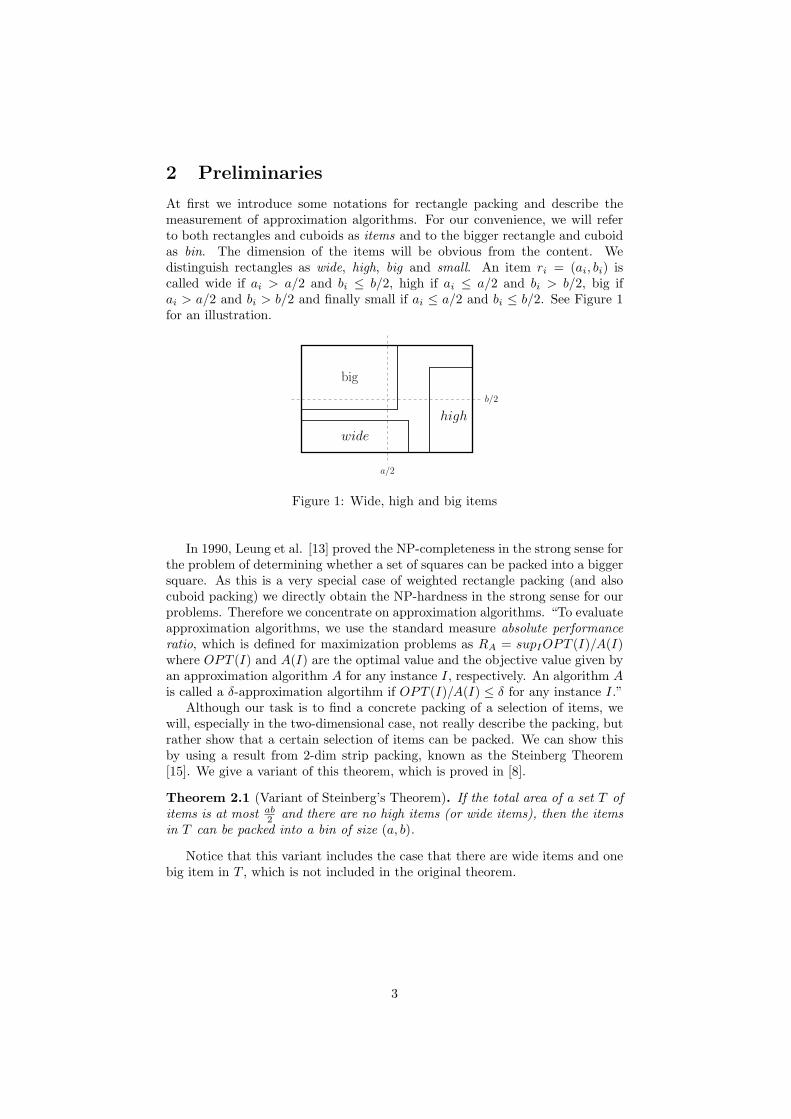
At first we introduce some notations for rectangle packing and describe themeasurement of approximation algorithms. For our convenience, we will referto both rectangles and cuboids as items and to the bigger rectangle and cuboidas bin. The dimension of the items will be obvious from the content. Wedistinguish rectangles as wide, high, big and small. An item ri = (ai, bi) iscalled wide if ai > a/2 and bi ≤ b/2, high if ai ≤ a/2 and bi > b/2, big ifai > a/2 and bi > b/2 and finally small if ai ≤ a/2 and bi ≤ b/2. See Figure 1for an illustration.

a/2

b/2

wide

high

big

Figure 1: Wide, high and big items

In 1990, Leung et al. [13] proved the NP-completeness in the strong sense forthe problem of determining whether a set of squares can be packed into a biggersquare. As this is a very special case of weighted rectangle packing (and alsocuboid packing) we directly obtain the NP-hardness in the strong sense for ourproblems. Therefore we concentrate on approximation algorithms. “To evaluateapproximation algorithms, we use the standard measure absolute performanceratio, which is defined for maximization problems as RA = supIOPT (I)/A(I)where OPT (I) and A(I) are the optimal value and the objective value given byan approximation algorithm A for any instance I, respectively. An algorithm Ais called a δ-approximation algortihm if OPT (I)/A(I) ≤ δ for any instance I.”

Although our task is to find a concrete packing of a selection of items, wewill, especially in the two-dimensional case, not really describe the packing, butrather show that a certain selection of items can be packed. We can show thisby using a result from 2-dim strip packing, known as the Steinberg Theorem[15]. We give a variant of this theorem, which is proved in [8].

Theorem 2.1 (Variant of Steinberg’s Theorem). If the total area of a set T ofitems is at most ab

2 and there are no high items (or wide items), then the itemsin T can be packed into a bin of size (a, b).

Notice that this variant includes the case that there are wide items and onebig item in T , which is not included in the original theorem.

3

3 A (2+ ε)- approximation algorithm for rectan-gle packing with profits

3.1 Introduction

At first we present some basic methods used to design algorithms for theoret-ical purposes. These methods focus on polynomial running time which mayunfortunately be of very high order. We present the enumeration, the con-stant packing and the linear programming method. Especially enumeration andconstant packing are not really of practical use.

Enumeration (guessing): Assume a polynomial number of cases, each ofwhich can be solved in polynomial time. Obviously we can compute all casesand therefore find an optimal solution in polynomial time. As we might want toenumerate the cases to do this, the method is called enumeration. Alternatively,we also use the guessing perspective. Hereby we guess an optimal solution froma polynomial number of cases. Actually this includes the exhaustive search ofthe enumeration. The advantage of this perspective is the possibility to use anoptimal solution in the description of our algorithm.

Constant packing: “For a constant number of items (bounded by N) thetest of the existence of a feasible packing takes constant time (exponentially inN). To see this, consider the following simple packing algorithm Bottom-Up(BU) for a list of items: When an item is packed, it is placed, left-justified atthe lowest possible level in the current packing. It is not difficult to observethat any optimal packing can be transferred into a packing generated by BUon a specified order of items. For N items, we can apply the algorithm BU toN ! different item lists (different orders). A feasible packing exists if and only ifBU gives one.”

Linear programming: As it is NP-hard to solve integer programs, we uselinear programming as a relaxation to find a selection of items with almost op-timal profit. Fractional solutions may occur and will be handled appropriately.In 1979 Khachiyan introduced the ellipsoid method as the first polynomial timealgorithm for linear programming [11]. Later Karmarkar introduced the moreefficient inner-point method [12].

We describe the (2 + ε)-algorithm in several steps starting with a very basicalgorithm which will reveal the main ideas. Afterwards we will subsequentlyadd more details.

3.2 First step - guessing the most profitable items, basicalgorithm

Let k be a constant. We suppose the existence of an optimal packing with morethan k items. The other case will be handled later.

Firstly, we guess the k most profitable items of an optimal packing, callingthem the candidate set S. As k is a constant, the number

(nk

)of possible can-

didate sets is polynomial and the guessing can be done in polynomial time. Weensure that the items of S can be packed into a bin by using the constant pack-ing method. All additionally packed items have profits bounded by minr∈S pr.

4

Later we will have more sophisticated estimations for this profit. Notice thatit is crucial that we guess the most profitable items of an optimal packing andnot just an arbitrary selection of packed items. Secondly, we construct a linearprogram to find a set X of additional items with small profits such that theoverall profit is almost optimal. Thirdly, we pack X ∪ S into two bins of size(a, b) by using our variant of Steinberg’s Theorem 2.1.

Our basic algorithm can be outlined as follows

1. guess the k most profitable items S of an optimal solution,

2. find a set X of additional items with almost optimal profit by solving alinear program,

3. pack X ∪ S into two bins of size (a, b) and choose the bin with the higherprofit.

We will become more specific soon. It should be plausible now, that we geta (2 + ε)-approximation because the profit of X ∪ S is almost optimal (whichmeans p(X ∪ S) ≥ (1 − ε)OPT (I)) and therefore the higher profit is at leastnear to the half of the optimum.

We might now ask why the first step is mandatory, if we can find the set Xwith a linear program. This is due to the discarding of some of the items of Xin later steps. Therefore we need to estimate the total loss of discarded items.

3.3 Second step - guessing the gap structure

Our aim is to construct constraints for the linear program that ensure, that wecan pack all the selected items into two bins. We derive constraints for the wideand for the high items separately but we do not consider the small items at themoment. For the sake of simplicity we consider the big items as high items.Exemplarily we describe the constraints for the wide items.

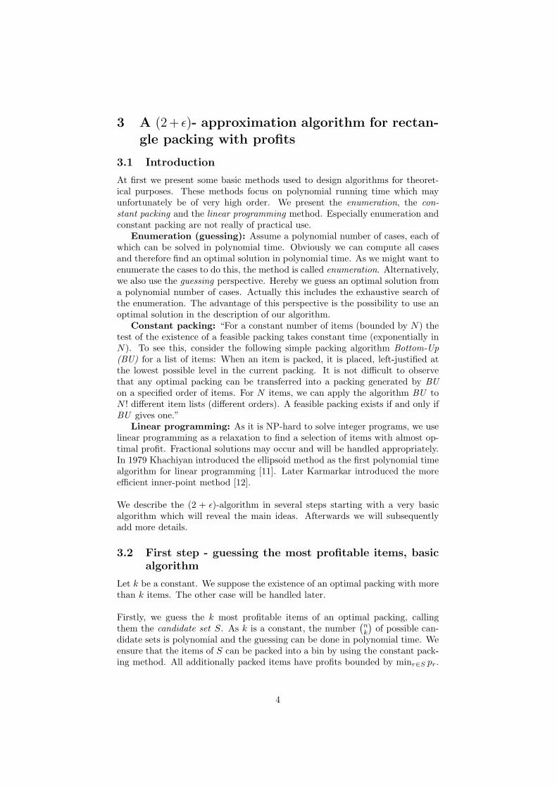
Although we obviously do not know an optimal packing it makes sense toexamine the structure of an optimal packing to derive properties we can use forthe construction of constraints. Suppose we know a packing P of an optimalsolution Lopt with the candidate set S - see Figure 2. We examine the gapstructure in the bin that is created by the items of the candidate set.

Figure 2: Packing P of an optimal solution Lopt with the candidate set S

5

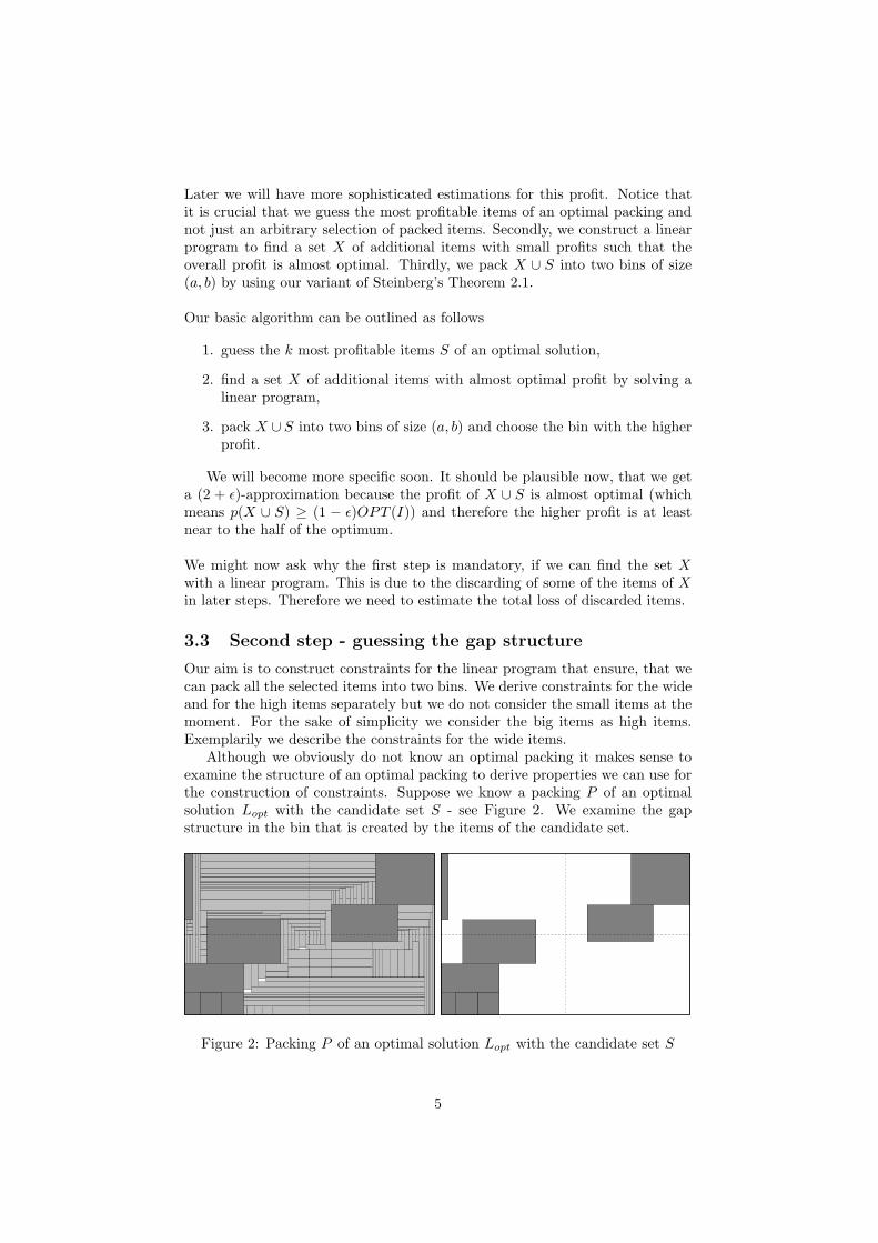
“To find the gaps in our packing P , use the following sweeping procedure.Remove all items that do not belong to the candidate set and start to sweepwith a horizontal line beginning with the lower boundary of (a, b). By sweepingfind the lower and upper boundary of each candidate rectangle r in S. Insert ahorizontal line to the left and right until it intersects another rectangle of S orends at the boundary of rectangle (a, b). At most 2|S| = 2k lines are inserted.This partitions the big rectangle (a, b) into rectangles of S and a set of emptyrectangles. Empty rectangles of width > a/2 are called wide gaps. Clearly,there is at most one gap of width > a/2 intersecting with a horizontal line.Therefore the number of wide gaps is bounded by 2|S|+1 = 2k +1 - see Figure3 for an illustration.”

wide gap

wide gap

wide gap

wide gap

wide gap

highgap

highgap

highgap

Figure 3: Gap structures of the wide and high gaps

It is clear, that additional wide items can only be contained in wide gaps -but they might overlap two or more wide gaps partially. We want to use thewide gaps, which we are going to guess later, to make up constraints for thelinear program. Therefore we have to ensure on the one hand, that every wideitem is interior to exactly one wide gap and on the other hand, that there isonly a polynomial number of cases to choose for the gaps, such that they canbe guessed.

As there are at most 2k + 1 wide gaps, there can be at most 2k additionalwide items in the optimal solution that overlap two or more gaps. We removethese items from the optimal solution Lopt - which makes Lopt suboptimal. Laterwe show, that Lopt is still almost optimal which is sufficient for us.

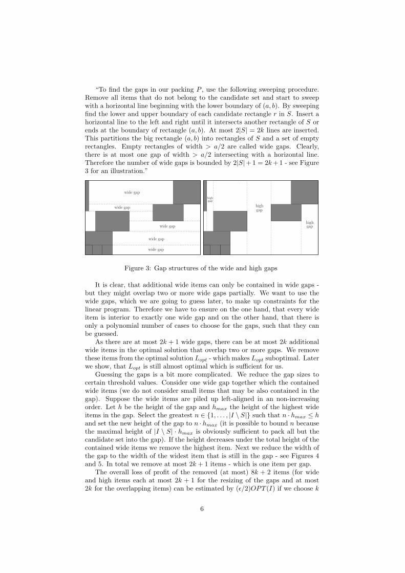
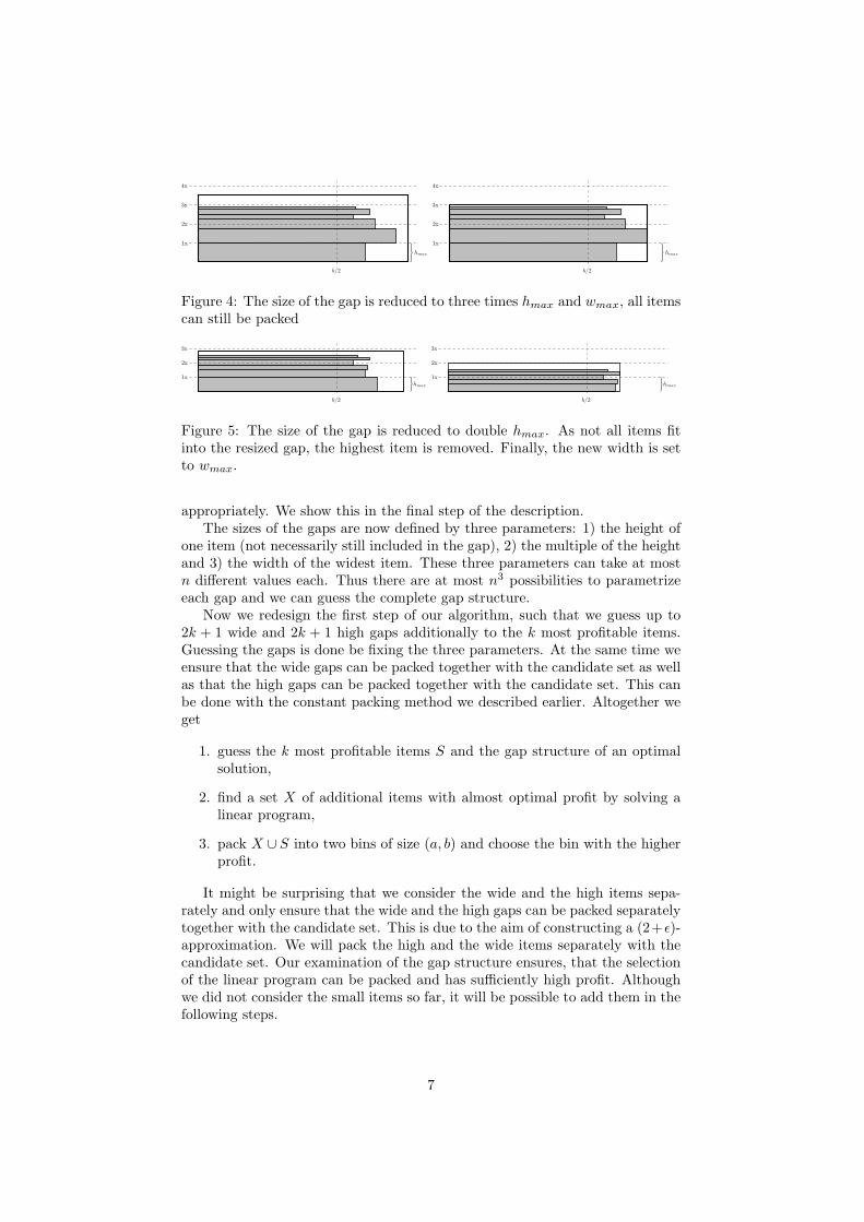
Guessing the gaps is a bit more complicated. We reduce the gap sizes tocertain threshold values. Consider one wide gap together which the containedwide items (we do not consider small items that may be also contained in thegap). Suppose the wide items are piled up left-aligned in an non-increasingorder. Let h be the height of the gap and hmax the height of the highest wideitems in the gap. Select the greatest n ∈ {1, . . . , |I \ S|} such that n · hmax ≤ hand set the new height of the gap to n · hmax (it is possible to bound n becausethe maximal height of |I \ S| · hmax is obviously sufficient to pack all but thecandidate set into the gap). If the height decreases under the total height of thecontained wide items we remove the highest item. Next we reduce the width ofthe gap to the width of the widest item that is still in the gap - see Figures 4and 5. In total we remove at most 2k + 1 items - which is one item per gap.

The overall loss of profit of the removed (at most) 8k + 2 items (for wideand high items each at most 2k + 1 for the resizing of the gaps and at most2k for the overlapping items) can be estimated by (ε/2)OPT (I) if we choose k

6

b/2

1x

2x

3x

4x

} hmax

b/2

1x

2x

3x

4x

} hmax

Figure 4: The size of the gap is reduced to three times hmax and wmax, all itemscan still be packed

b/2

1x

2x

3x

}hmax

b/2

1x

2x

3x

}hmax

Figure 5: The size of the gap is reduced to double hmax. As not all items fitinto the resized gap, the highest item is removed. Finally, the new width is setto wmax.

appropriately. We show this in the final step of the description.The sizes of the gaps are now defined by three parameters: 1) the height of

one item (not necessarily still included in the gap), 2) the multiple of the heightand 3) the width of the widest item. These three parameters can take at mostn different values each. Thus there are at most n3 possibilities to parametrizeeach gap and we can guess the complete gap structure.

Now we redesign the first step of our algorithm, such that we guess up to2k + 1 wide and 2k + 1 high gaps additionally to the k most profitable items.Guessing the gaps is done be fixing the three parameters. At the same time weensure that the wide gaps can be packed together with the candidate set as wellas that the high gaps can be packed together with the candidate set. This canbe done with the constant packing method we described earlier. Altogether weget

1. guess the k most profitable items S and the gap structure of an optimalsolution,

2. find a set X of additional items with almost optimal profit by solving alinear program,

3. pack X ∪ S into two bins of size (a, b) and choose the bin with the higherprofit.

It might be surprising that we consider the wide and the high items sepa-rately and only ensure that the wide and the high gaps can be packed separatelytogether with the candidate set. This is due to the aim of constructing a (2+ε)-approximation. We will pack the high and the wide items separately with thecandidate set. Our examination of the gap structure ensures, that the selectionof the linear program can be packed and has sufficiently high profit. Althoughwe did not consider the small items so far, it will be possible to add them in thefollowing steps.

7

3.4 Third step - integer program

Where did our considerations lead us so far? For every optimal solution there is arestricted solution with almost the same profit (OPTres(I) ≥ (1− ε/2)OPT (I))and the property, that all wide items are interior to the wide gaps and canadditionally be packed into insignificantly downsized gaps. We can guess thesedownsized gaps and use them in the constraints of the linear program. Natu-rally the same applies to the high items and high gaps.

Suppose we guessed a candidate set S and additionally W ≤ 2k + 1 wide gaps(aw

i , bwi ) and H ≤ 2k + 1 high gaps (ah

i , bhi ). Separate the remaining items into

the sets Rw ⊂ I \ S of wide items, Rh ⊂ I \ S of high items and Rs ⊂ I \ Sof small items. Each item in Rw, Rh and Rs has profit at most minr∈Spr. Foreach wide item r we define a set Gw

r of potential gaps g with ar ≤ awg . Similarly,

we define Ghr for high items r with gaps g such that br ≤ bh

g .For each wide (high) item r and each wide (high) gap g ∈ Gw

r (g ∈ Ghr ) we

introduce a variable xr,g ∈ {0, 1} where

xr,g ={

1, if r is placed in gap g0, otherwise.

For each small item r we use a variable xr ∈ {0, 1} where

xr ={

1, if r is selected0, otherwise.

Our objective is to maximize the profit, which is the sum of the profits from thecandidate set S and the selected items from the sets Rw, Rh und Rs. Formally

max∑r∈S

pr︸ ︷︷ ︸candidate set S

+∑

r∈Rw

pr

∑g∈Gw

r

xr,g︸ ︷︷ ︸wide items Rw

+∑

r∈Rh

pr

∑g∈Gh

r

xr,g︸ ︷︷ ︸high items Rh

+∑

r∈Rs

pr · xr︸ ︷︷ ︸small items Rs

Due to the guessing of the gap structure we get two constraints for bothwide and high items. First, every wide item can be packed at most in one widegap and second, the total height of wide items in a wide gap is bounded bythe height of that gap. For the wide items and wide gaps we get the followingconstraints ∑

g∈Gwr

xr,g ≤ 1 r ∈ Rw

∑r∈Rw, ar≤aw

g

brxr,g ≤ bwg 1 ≤ g ≤ W

and similar for high gaps and high items∑g∈Gh

r

xr,g ≤ 1 r ∈ Rh

∑r∈Rh, br≤bh

g

arxr,g ≤ ahg 1 ≤ g ≤ H

8

Finally we add a constraint on the space to bound the selection of small items.The total area of the selected items may not exceed the bin size.∑

r∈S

arbr︸ ︷︷ ︸candidate set S

+∑

r∈Rw

arbr

∑g∈Gw

r

xr,g︸ ︷︷ ︸wide items Rw

+∑

r∈Rh

arbr

∑g∈Gh

r

xr,g︸ ︷︷ ︸high items Rh

+∑

r∈Rs

arbr · xr︸ ︷︷ ︸small items Rs

≤ ab

In fact the area of the candidate set is constant, as we guessed the set before-hand. Thus this constant can be computed with the right hand side of theinequality.

Adding the integer constraint we get the following integer program

max∑r∈S

pr +∑

r∈Rw

pr

∑g∈Gw

r

xr,g +∑

r∈Rh

pr

∑g∈Gh

r

xr,g +∑

r∈Rs

pr · xr

such that ∑g∈Gw

r

xr.g ≤ 1 r ∈ Rw

∑g∈Gh

r

xr,g ≤ 1 r ∈ Rh

∑r∈Rw, ar≤aw

g

brxr,g ≤ bwg 1 ≤ g ≤ W

∑r∈Rh, br≤bh

g

arxr,g ≤ ahg 1 ≤ g ≤ H

∑r∈S

arbr +∑

r∈Rw

arbr

∑g∈Gw

r

xr,g +∑

r∈Rh

arbr

∑g∈Gh

r

xr,g +∑

r∈Rs

arbr · xr ≤ ab

xr,g ∈ {0, 1} r ∈ Rw, g ∈ Gwr

xr,g ∈ {0, 1} r ∈ Rh, g ∈ Ghr

xr ∈ {0, 1} r ∈ Rs

Relaxing the integer constraints to xr,g ∈ [0, 1] and xr ∈ [0, 1] we derive alinear program. Of course we have to adapt the interpretation of the variablesto

xr,g = fraction of r that is placed in gap g

xr = fraction of r that is selected.

Recall that an optimal solution (x∗r,g, x∗r) of the linear program can be

found in polynomial time and notice that the profit P ∗ of this solution is atleast as big as the profit of the restricted solution OPTres(I) and thereforeP ∗ ≥ (1 − ε/2)OPT (I). Now we have to transform this, possibly fractional,solution into an integer solution without losing to much profit. This is doneby a reduction to job scheduling on unrelated machines with costs which wepresent for the wide items:

9

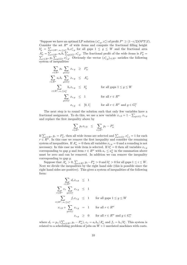
“Suppose we have an optimal LP solution (x∗r,g, x∗r) of profit P ∗ ≥ (1−ε/2)OPT (I).

Consider the set Rw of wide items and compute the fractional filling heightb∗g =

∑r∈Rw, ar≤aw

gbrx

∗r,g for all gaps 1 ≤ g ≤ W and the fractional area

A∗w =

∑r∈Rw arbr

∑g∈Gw

rx∗r.g. The fractional profit of the wide items is P ∗

w =∑r∈Rw pr

∑g∈Gw

rx∗r.g. Obviously the vector (x∗r,g)r∈Rw satisfies the following

system of inequalities∑r∈Rw

pr

∑g∈Gw

r

xr.g ≥ P ∗w∑

r∈Rw

arbr

∑g∈Gw

r

xr.g ≤ A∗w∑

r∈Rw, ar≤awg

brxr,g ≤ b∗g for all gaps 1 ≤ g ≤ W

∑g∈Gw

r

xr,g ≤ 1 for all r ∈ Rw

xr,g ∈ [0, 1] for all r ∈ Rw and g ∈ Gwr

The next step is to round the solution such that only few variables have afractional assignment. To do this, we use a new variable xr,0 = 1−

∑g∈Gw

rxr,g

and replace the first inequality above by∑r∈Rw

prxr,0 ≤∑

r∈Rw

pr − P ∗w

If∑

r∈Rw pr = P ∗w, then all wide items are selected and

∑i∈Gw

rx∗r,i = 1 for each

r ∈ Rw. In this case we remove the first inequality and consider the remainingsystem of inequalities. If A∗

w = 0 then all variables xr,g = 0 and a rounding is notnecessary. In this case no wide item is selected. If b∗i = 0 then all variables xr,g

corresponding to gap g and item r ∈ Rw with ar ≤ awg in the summation above

must be zero and can be removed. In addition we can remove the inequalitycorresponding to gap g.

Suppose that A∗w > 0,

∑r∈Rw pr−P ∗

w > 0 and b∗i > 0 for all gaps 1 ≤ i ≤ W .Next we divide the inequalities by the right hand side (this is possible since theright hand sides are positive). This gives a system of inequalities of the followingform: ∑

r∈Rw

drxr,0 ≤ 1∑r∈Rw

er

∑g∈Gw

r

xr.g ≤ 1

∑r∈Rw, ar≤aw

i

frxr,g ≤ 1 for all gaps 1 ≤ g ≤ W

xr,0 +∑

g∈Gwr

xr,g = 1 for all r ∈ Rw

xr,g ≥ 0 for all r ∈ Rw and g ∈ Gwr

where dr = pr/(∑

r∈Rw pr − P ∗w), er = arbr/A

∗w and fr = br/b∗i . This system is

related to a scheduling problem of jobs on W +1 unrelated machines with costs.

10

The first inequality is related to the cost of the solution and minimizing the costgives a feasible solution. The next W +1 inequalities are related to the machines1, . . . ,W + 1. One can round a fractional solution of this system in polynomialtime to another solution with optimum cost and at most W fractional jobs [14],[6]. Removing these fractional items after the rounding and using the same ideafor the high and small items gives an integral solution where we have removedat most W + H + 1 ≤ 4k + 3 items. Notice, that we have no inequalities forgaps for the small items. Therefore we remove at most 1 small item.”

As in the last section we removed a number of items in this step. The totalprofit of these items can also be bound by (ε/2)OPT as we show later. Thecurrent state of our algorithm is as follows

1. guess the k most profitable items S and the gap structure of an optimalsolution,

2. find a fractional solution of the linear program with almost optimal profit,

3. round the fractional solution to a selection of items X,

4. pack X ∪ S into two bins of size (a, b) and choose the bin with the higherprofit.

3.5 Fourth step - packing

In this chapter the packing of the items corresponding to the integer solutioninto two bins is described. From the result of our integer solution we know howto pack either the wide items or the high items together with the candidate setinto a bin. We only need to pile up the wide (high) items into the correspondinggaps and pack the constant number of candidate items and gaps into the bin(we verified that this is possible in the second step).

Let X be the set of additional items from the integer solution. We can split Xinto three set Xw, Xh and Xs of wide, high and small items respectively (recallthat a probably included big item is considered as high one). We distributethese items to the sets Tw and Th which represent the two bins in which wewant to pack. Let P be the total profit of the items S ∪X.

“First, we submit S to both sets Tw and Th. Second, we add Xw to Tw

and Xh to Th. If either p(Tw) ≥ P/2 or p(Th) ≥ P/2 we pack the set with thehigher profit into a bin. This is possible due to the remark above. Otherwisep(Tw) < P/2 and p(Th) < P/2. In this case we have to add the small items inXs to our sets. Therefore we can not use the gap structure to pack the bins anylonger. Instead we use the variant of Steinberg’s Theorem (Theorem 2.1). Thisis possible because we separated the wide and high items into different sets.

If the area s(Tw) > ab/2 then the area of the other items is s(Th ∪ Xs) ≤ab/2. Therefore we can use our variant of Steinberg’s Theorem to pack the itemsof Xs and Th together into one bin. The profit of these items is p(Th ∪ Xs) >P/2. The other case (s(Th) > ab/2) is packed similarly.

Suppose now that s(Tw) ≤ ab/2 and s(Th) ≤ ab/2. We distribute the smallitems of Xs into three sets Xs

T w , XsT h and X∗ such that s(Tw ∪ Xs

T w) ≤ ab/2,s(Th ∪Xs

T h) ≤ ab/2 and |X∗| = 1. This can be done easily in a greedy manner.

11

Let X∗ = {r}. From the sets Tw∪XsT w and Th∪Xs

T h we choose the one with thehigher profit and pack it, using the variant of Steinberg’s Theorem, into a bin.In the last step we will show that the profit is ≥ P/2−pr ≥ (1−ε)OPT (I)/2.”

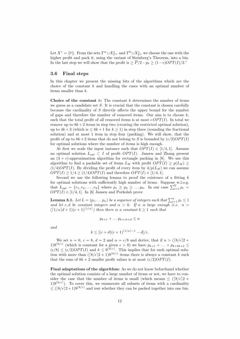
3.6 Final steps

In this chapter we present the missing bits of the algorithms which are thechoice of the constant k and handling the cases with an optimal number ofitems smaller than k.

Choice of the constant k: The constant k determines the number of itemswe guess as a candidate set S. It is crucial that the constant is chosen carefullybecause the cardinality of S directly affects the upper bound for the numberof gaps and therefore the number of removed items. Our aim is to choose k,such that the total profit of all removed items is at most ε OPT (I). In total weremove up to 8k+2 items in step two (creating the restricted optimal solution),up to 4k +3 (which is ≤ 8k +1 for k ≥ 1) in step three (rounding the fractionalsolution) and at most 1 item in step four (packing). We will show, that theprofit of up to 8k +2 items that do not belong to S is bounded by (ε/2)OPT (I)for optimal solutions where the number of items is high enough.

At first we scale the input instance such that OPT (I) ∈ [1/4, 1]. Assumean optimal solution Lopt ⊂ I of profit OPT (I). Jansen and Zhang presentan (3 + ε)-approximation algorithm for rectangle packing in [8]. We use thisalgorithm to find a packable set of items LH with profit OPT (I) ≥ p(LH) ≥(1/4)OPT (I). By dividing the profit of every item by 4/p(LH) we can assumeOPT (I) ≥ 1/4 ≥ (1/4)OPT (I) and therefore OPT (I) ∈ [1/4, 1].

Second we use the following lemma to proof the existence of a fitting kfor optimal solutions with sufficiently high number of items. Suppose w.l.o.g.that Lopt = {r1, r2, . . . , rn} where p1 ≥ p2 ≥ . . . pn. In our case

∑ni=1 pr =

OPT (I) ∈ [1/4, 1]. In [6] Jansen and Porkolab prove

Lemma 3.1. Let L = (p1, . . . pn) be a sequence of integers such that∑n

i=1 pi ≤ 1and let c, d be constant integers and α > 0. If n is large enough (i.e. n >(d1/αed + 1)(c + 1)d1/αe) then there is a constant k ≥ 1 such that

pk+1 + . . . pk+ck+d ≤ α

andk ≤ [(c + d)(c + 1)d1/αe−1 − d]/c.

We set n = n, c = 8, d = 2 and α = ε/8 and derive, that if n > (d8/εe2 +1)9d8/εe (which is constant for a given ε > 0) we have pk+1 + . . . + pk+8k+2 ≤(ε/8) ≤ (ε/2)OPT (I) and k ≤ 9d8/εe. This implies that for each optimal solu-tion with more than (d8/εe2 + 1)9d8/εe items there is always a constant k suchthat the sum of 8k + 2 smaller profit values is at most (ε/2)OPT (I).

Final adaptations of the algorithm: As we do not know beforehand whetherthe optimal solution consists of a large number of items or not, we have to con-sider the case that the number of items is small (which means ≤ (d8/εe2 +1)9d8/εe). To cover this, we enumerate all subsets of items with a cardinality≤ (d8/εe2+1)9d8/εe and test whether they can be packed together into one bin.

12

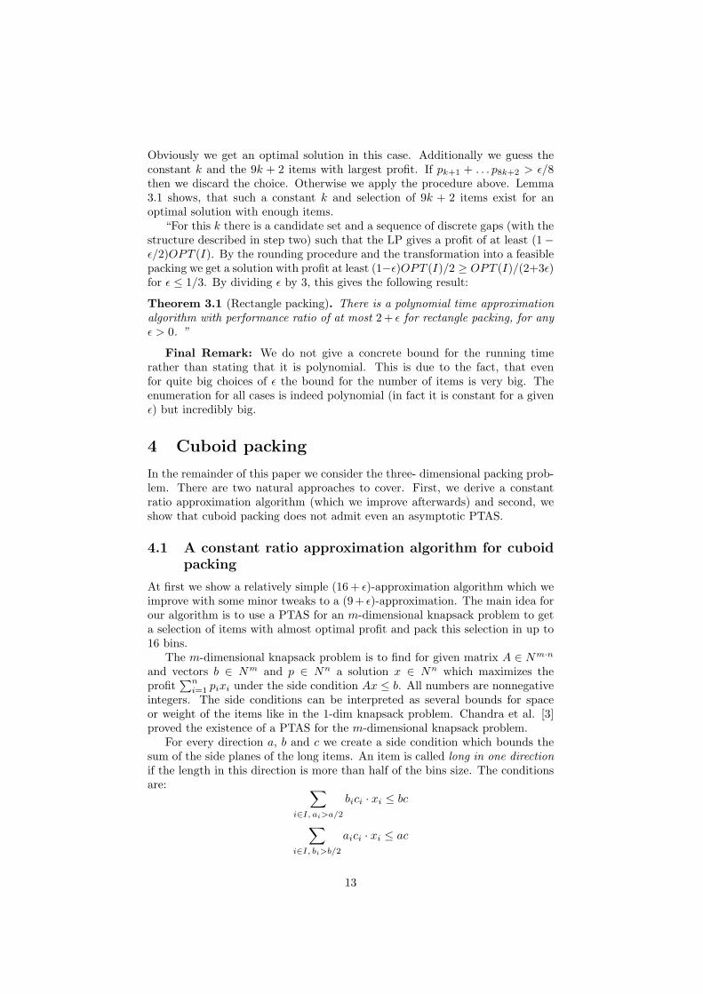
Obviously we get an optimal solution in this case. Additionally we guess theconstant k and the 9k + 2 items with largest profit. If pk+1 + . . . p8k+2 > ε/8then we discard the choice. Otherwise we apply the procedure above. Lemma3.1 shows, that such a constant k and selection of 9k + 2 items exist for anoptimal solution with enough items.

“For this k there is a candidate set and a sequence of discrete gaps (with thestructure described in step two) such that the LP gives a profit of at least (1−ε/2)OPT (I). By the rounding procedure and the transformation into a feasiblepacking we get a solution with profit at least (1−ε)OPT (I)/2 ≥ OPT (I)/(2+3ε)for ε ≤ 1/3. By dividing ε by 3, this gives the following result:

Theorem 3.1 (Rectangle packing). There is a polynomial time approximationalgorithm with performance ratio of at most 2 + ε for rectangle packing, for anyε > 0. ”

Final Remark: We do not give a concrete bound for the running timerather than stating that it is polynomial. This is due to the fact, that evenfor quite big choices of ε the bound for the number of items is very big. Theenumeration for all cases is indeed polynomial (in fact it is constant for a givenε) but incredibly big.

4 Cuboid packing

In the remainder of this paper we consider the three- dimensional packing prob-lem. There are two natural approaches to cover. First, we derive a constantratio approximation algorithm (which we improve afterwards) and second, weshow that cuboid packing does not admit even an asymptotic PTAS.

4.1 A constant ratio approximation algorithm for cuboidpacking

At first we show a relatively simple (16 + ε)-approximation algorithm which weimprove with some minor tweaks to a (9+ ε)-approximation. The main idea forour algorithm is to use a PTAS for an m-dimensional knapsack problem to geta selection of items with almost optimal profit and pack this selection in up to16 bins.

The m-dimensional knapsack problem is to find for given matrix A ∈ Nm·n

and vectors b ∈ Nm and p ∈ Nn a solution x ∈ Nn which maximizes theprofit

∑ni=1 pixi under the side condition Ax ≤ b. All numbers are nonnegative

integers. The side conditions can be interpreted as several bounds for spaceor weight of the items like in the 1-dim knapsack problem. Chandra et al. [3]proved the existence of a PTAS for the m-dimensional knapsack problem.

For every direction a, b and c we create a side condition which bounds thesum of the side planes of the long items. An item is called long in one directionif the length in this direction is more than half of the bins size. The conditionsare: ∑

i∈I, ai>a/2

bici · xi ≤ bc

∑i∈I, bi>b/2

aici · xi ≤ ac

13

∑i∈I, ci>c/2

aibi · xi ≤ ab

A fourth and fifth condition is added in order to limit the total space used byall items and the number of big items, respectively.∑

i∈I

aibici · xi ≤ abc

∑i∈I ai>a/2 bi>b/2 ci>c/2

xi ≤ 1

The objective remains untouched: ∑i∈I

pixi

Remark: In fact this resembles the construction of the integer program wederived in the previous sections. But as we only use upper bounds and a constantnumber of constraints, we can regard this as a m-dim knapsack problem andtherefore solve it directly instead of having to round the fractional solution of alinear relaxation. A similar idea is used in [8] to derive a (3 + ε)-approximationfor the rectangle packing.

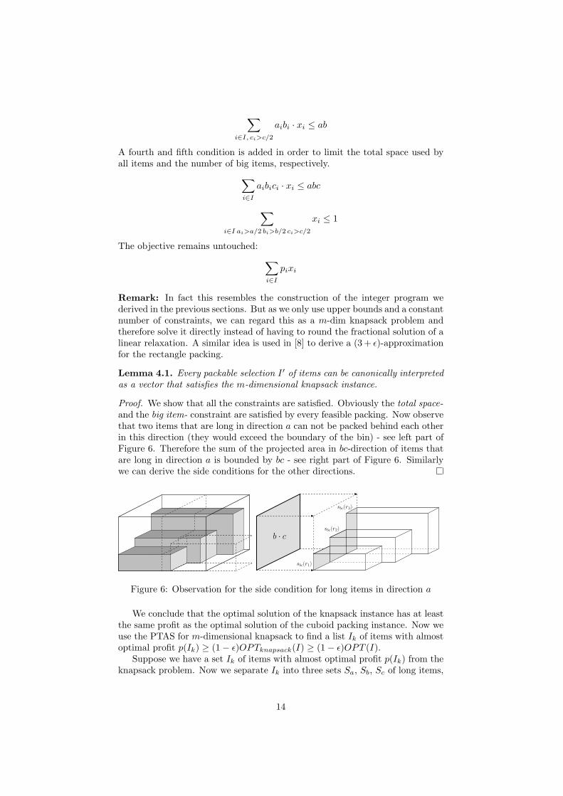
Lemma 4.1. Every packable selection I ′ of items can be canonically interpretedas a vector that satisfies the m-dimensional knapsack instance.

Proof. We show that all the constraints are satisfied. Obviously the total space-and the big item- constraint are satisfied by every feasible packing. Now observethat two items that are long in direction a can not be packed behind each otherin this direction (they would exceed the boundary of the bin) - see left part ofFigure 6. Therefore the sum of the projected area in bc-direction of items thatare long in direction a is bounded by bc - see right part of Figure 6. Similarlywe can derive the side conditions for the other directions.

b · c

sbc(r3)

sbc(r2)

sbc(r1)

Figure 6: Observation for the side condition for long items in direction a

We conclude that the optimal solution of the knapsack instance has at leastthe same profit as the optimal solution of the cuboid packing instance. Now weuse the PTAS for m-dimensional knapsack to find a list Ik of items with almostoptimal profit p(Ik) ≥ (1− ε)OPTknapsack(I) ≥ (1− ε)OPT (I).

Suppose we have a set Ik of items with almost optimal profit p(Ik) from theknapsack problem. Now we separate Ik into three sets Sa, Sb, Sc of long items,

14

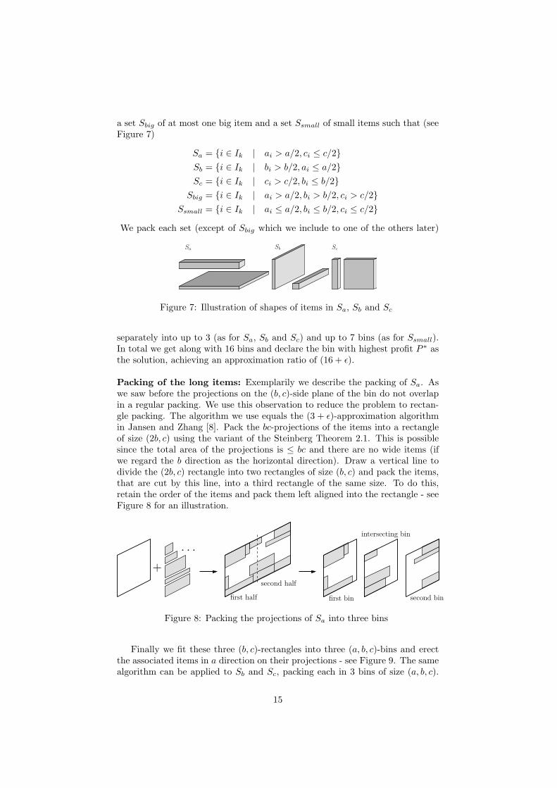
a set Sbig of at most one big item and a set Ssmall of small items such that (seeFigure 7)

Sa = {i ∈ Ik | ai > a/2, ci ≤ c/2}Sb = {i ∈ Ik | bi > b/2, ai ≤ a/2}Sc = {i ∈ Ik | ci > c/2, bi ≤ b/2}

Sbig = {i ∈ Ik | ai > a/2, bi > b/2, ci > c/2}Ssmall = {i ∈ Ik | ai ≤ a/2, bi ≤ b/2, ci ≤ c/2}

We pack each set (except of Sbig which we include to one of the others later)

Sa Sb Sc

Figure 7: Illustration of shapes of items in Sa, Sb and Sc

separately into up to 3 (as for Sa, Sb and Sc) and up to 7 bins (as for Ssmall).In total we get along with 16 bins and declare the bin with highest profit P ∗ asthe solution, achieving an approximation ratio of (16 + ε).

Packing of the long items: Exemplarily we describe the packing of Sa. Aswe saw before the projections on the (b, c)-side plane of the bin do not overlapin a regular packing. We use this observation to reduce the problem to rectan-gle packing. The algorithm we use equals the (3 + ε)-approximation algorithmin Jansen and Zhang [8]. Pack the bc-projections of the items into a rectangleof size (2b, c) using the variant of the Steinberg Theorem 2.1. This is possiblesince the total area of the projections is ≤ bc and there are no wide items (ifwe regard the b direction as the horizontal direction). Draw a vertical line todivide the (2b, c) rectangle into two rectangles of size (b, c) and pack the items,that are cut by this line, into a third rectangle of the same size. To do this,retain the order of the items and pack them left aligned into the rectangle - seeFigure 8 for an illustration.

. . .

+

first half

second half

first bin second bin

intersecting bin

Figure 8: Packing the projections of Sa into three bins

Finally we fit these three (b, c)-rectangles into three (a, b, c)-bins and erectthe associated items in a direction on their projections - see Figure 9. The samealgorithm can be applied to Sb and Sc, packing each in 3 bins of size (a, b, c).

15

As Sbig contains at most one item it can be packed together with any of thesets Sa, Sb or Sc - see the note on the variant of the Steinberg’s Theorem 2.1.

Figure 9: Erecting the items of Sa on the pattern of their projections

Packing of the small items: To pack the set of small items Ssmall weuse a combination of rectangle packing with Steinberg and a layer packinginto an unlimited 3-dim strip similar to the simple 2-dim algorithm Next-Fit-Decreasing-Height (NFDH) which orders the items in non-increasing height andfills the strip in layers. First, we order the items in non-increasing heightc1 ≥ c2 ≥ . . . ≥ ck. Second, we group the items such that the sum of theab-size of each group is as close to ab/2 as possible. Formally, we define vari-ables g1, . . . gl such that g1 = 1 and

Si =gi+1−1∑j=gi

ajbj ≤ ab/2 for all 1 ≤ i ≤ l − 1 and

gi+1∑j=gi

ajbj > ab/2 for all 1 ≤ i ≤ l − 1 and

Si =k∑

j=gl

ajbj ≤ ab/2

As all the items are small, the ab-area of each item is ≤ ab/4. Therefore Si ≥ab/4 for all 1 ≤ i ≤ l − 1. Furthermore the ab-projection of each group Gi =(gi, gi + 1, . . . , gi+1 − 1) of items can be packed into a rectangle of size (a, b)with Steinberg’s algorithm, as their total area is bounded by ab/2 and thereare neither wide nor high items. As for the large items we can erect the smallitems on their projection and therefore pack each group Gi into one layer ofsize (a, b, cgi

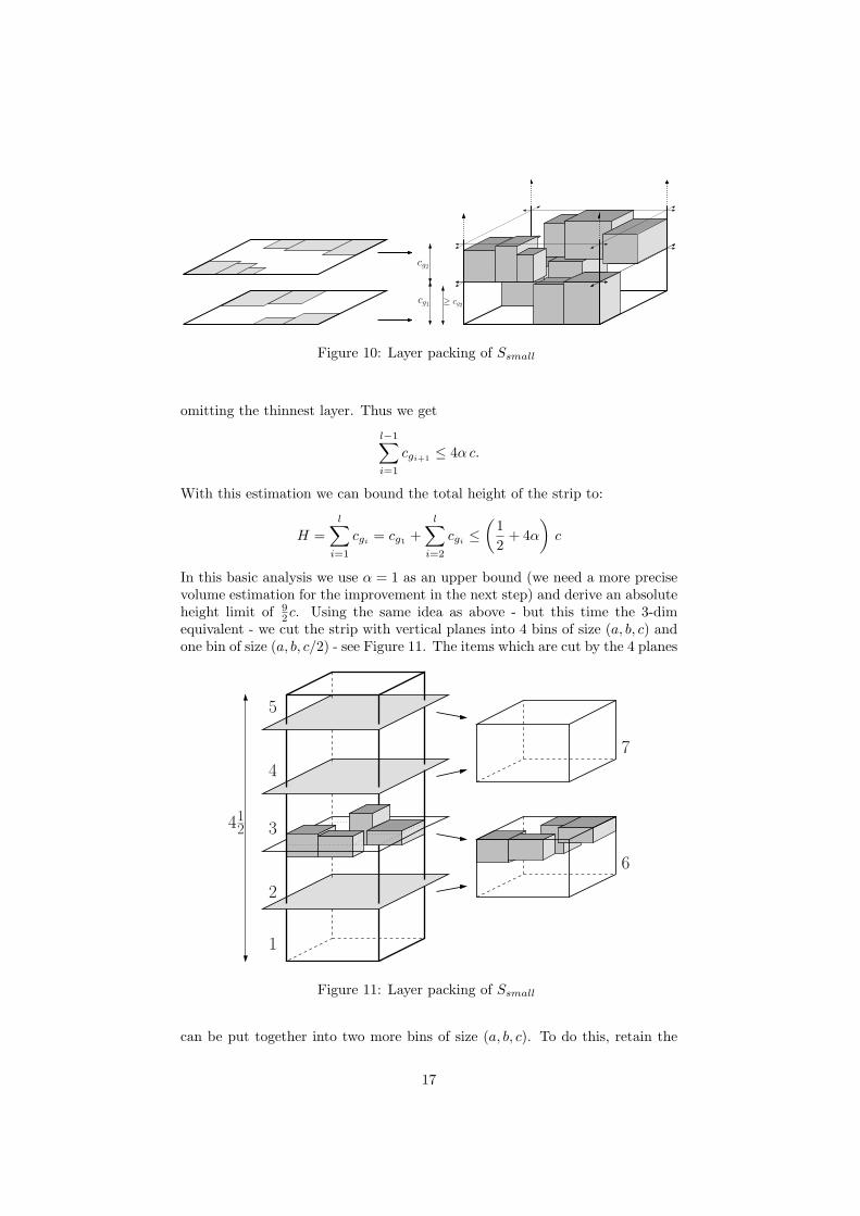
) with the highest heigh in that group. Insert the layers in non-increasing order into a strip with the basis (a, b) and unlimited height - seeFigure 10.

We analyse the height of this strip packing. Suppose the total volume ofsmall items is bounded by V =

∑i∈Ssmall

aibici ≤ α abc. In every layer 1 ≤i ≤ l − 1 all items have a c-length of at least cgi+1 . Hence, the filling of everylayer can be estimated by the height of the succeeding layer. Therefore the totalvolume can be estimated by

V ≥l−1∑i=1

cgi+1Si ≥l−1∑i=1

cgi+1ab/4

16

cg1

cg2

≥ cg2

Figure 10: Layer packing of Ssmall

omitting the thinnest layer. Thus we get

l−1∑i=1

cgi+1 ≤ 4α c.

With this estimation we can bound the total height of the strip to:

H =l∑

i=1

cgi= cg1 +

l∑i=2

cgi≤

(12

+ 4α

)c

In this basic analysis we use α = 1 as an upper bound (we need a more precisevolume estimation for the improvement in the next step) and derive an absoluteheight limit of 9

2c. Using the same idea as above - but this time the 3-dimequivalent - we cut the strip with vertical planes into 4 bins of size (a, b, c) andone bin of size (a, b, c/2) - see Figure 11. The items which are cut by the 4 planes

2

3

4

5

1

6

7

412

Figure 11: Layer packing of Ssmall

can be put together into two more bins of size (a, b, c). To do this, retain the

17

order of the intersections on two of the cutting planes and insert them bottomaligned and top aligned respectively into one bin. As the c-length is boundedby c/2 the items do not overlap. Thus we can pack Ssmall into at most 7 binswhich proves

Theorem 4.1 (Cuboid packing). There is a polynomial time approximationalgorithm with performance ratio of at most 16 + ε for cuboid packing, for anyε > 0.

4.2 Improvement

As already mentioned in the modified abstract, Lemma 4.2, which isbasic for the improvement of the algorithm, is not correct. Never-theless the idea of separating the items into Sa, Sb, Sc, Sbig and Ssmall

and the Observation 1 are still correct and are used in [4] to de-rive a (9 + ε)- and a (8 + ε)-approximation. Furthermore the idea ofusing placeholder items might still be useful for improving on theseresults.

The basic (16+ε)-approximation algorithm finds a selection of items with the m-dimensional knapsack and packs this selection into up to 16 bins. This methodis adopted from the (3 + ε)-algorithm for rectangle packing in [8]. It is notsurprising, that the algorithm can be improved by using the (2+ ε)-algorithm ofthe previous part of this paper. To do this we have to change our perspective.We can not longer pack all items into a certain number of bins, but separate theselection into several sets of items and apply ‘as good as possible’-approximationalgorithms on them. Therefore we need the following lemma

Lemma 4.2. Given a set of items S which fulfills the m-dimensional knapsackinstance of the previous section, an algorithm P that produces a partition S1 ∪S2 ∪ . . . ∪ Sl = S and a list of approximation algorithms A1, A2, . . . , Al whichhave an approximation ratio of δ1, δ2, . . . , δl on S1, S2, . . . , Sl, respectively, thereis an approximation algorithm A for cuboid packing with approximation ratio atmost δ1 + δ2 + . . . + δl + ε for every ε > 0.

Proof. Let A be the algorithm which first finds a selection of items S with them-dimensional knapsack of the previous section, using ε′ = ε/(δ1 +δ2 + . . .+δl).Then it applies P on S and Ai on Si for 1 ≤ i ≤ l. Let Si be the outputof the algorithm Ai. A outputs max(p(S1), p(S2), . . . , p(Sl)) together with thecorresponding packing. We prove that OPT (I) ≤ (δ1 + δ2 + . . . + δl + ε)A(I).

OPT (I) ≤ (1 + ε′)p(S)= (1 + ε′)(p(S1) + p(S2) + . . . + p(Sl))≤ (1 + ε′)(δ1p(S1) + δ2p(S2) + . . . + δlp(Sl))≤ (1 + ε′)(δ1 + δ2 + . . . + δl) max(p(S1), p(S2), . . . , p(Sl))= (δ1 + δ2 + . . . + δl + ε)A(I)

The mistake in this prove is that p(Si) ≤ δip(Si) doesn’t hold. In-stead we have OPT (Si) ≤ δip(Si). The former equation would only be

18

true, if algorithm Ai packed all items Si into the bins, which is nottrue for the (2 + ε) algorithm.

Notice, that the final ε can also absorb other arbitrarily small number in theapproximation ratios of A1, . . . , Al. The algorithm P is only needed to ensurelater, that the sets Si have certain properties from which the algorithm Ai canbenefit.

The main idea of the improved algorithm is to consider the volumes of thedifferent sets. Obviously the strip height of Ssmall decreases if the volume ofthese items is smaller. We make two observations before we give the algorithm.

Observation 1 (Packing small volume of Sa). Sa can be packed into one binif V ol(Sa) ≤ 1

4 abc.

Proof: If V ol(Sa) ≤ 14 abc then Sbc(Sa) ≤ 1

2 bc where Sbc(Sa) is the sum ofthe bc-side planes of the items in Sa. As there are no high item in Sa (whichmeans long in direction c), the bc- projections of the items can be packed intoone bin of size (b, c) with Steinbergs algorithm. Finally the items can be erectedin a- direction as usual. Obviously the same applies to the sets Sb and Sc andwe can include Sbig to any of these sets.

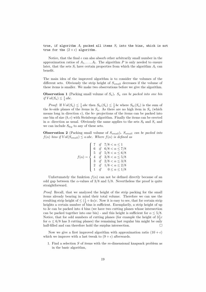
Observation 2 (Packing small volume of Ssmall). Ssmall can be packed intof(α) bins if V ol(Ssmall) ≤ α abc. Where f(α) is defined as

f(α) =

7 if 7/8 < α ≤ 16 if 6/8 < α ≤ 7/85 if 5/8 < α ≤ 6/84 if 3/8 < α ≤ 5/83 if 2/8 < α ≤ 3/82 if 1/8 < α ≤ 2/81 if 0 ≤ α ≤ 1/8

Unfortunately the funktion f(α) can not be defined directly because of anodd gap between the α-values of 3/8 and 5/8. Nevertheless the proof is quitestraightforward.

Proof. Recall, that we analyzed the height of the strip packing for the smallitems already bearing in mind their total volume. Therefore we can use theresulting strip height of ≤ ( 1

2 +4α)c. Now it is easy to see, that for certain stripheights a certain number of bins is sufficient. Exemplarily, a strip height of upto 3c can be packed into 4 bins (we have two cutting planes whose intersectioncan be packed together into one bin) - and this height is sufficient for α ≤ 5/8.Notice, that for odd numbers of cutting planes (for example the height of 31

2cfor α ≤ 6/8 has 3 cutting planes) the remaining last regular bin might be onlyhalf-filled and can therefore hold the surplus intersection.

Now we give a first improved algorithm with approximation ratio (10 + ε)which we improve with a last tweak to (9 + ε) afterwards.

1. Find a selection S of items with the m-dimensional knapsack problem asin the basic algorithm,

19

2. separate the items in S into the sets Sa, Sb, Sc and Ssmall as defined above(but consider a potential big item belonging to Sa),

3. if V ol(Sa) ≤ 1/4 abc than pack Sa into one bin, otherwise use the (2 + ε)-algorithm for rectangle packing for the bc-projection and erect the itemson the pattern (deal similarly with Sb and Sc),

4. pack Ssmall into a strip and transfer the strip into a minimal number ofbins according to f(α),

5. choose the bin with the highest profit.

Analysis: We consider four different cases:

1. V ol(Sa), V ol(Sb), V ol(Sc) ≤ 1/4 abcIn this case we need 3 bins for Sa, Sb and Sc and (like in the basis algo-rithm) 7 bins for Ssmall - summing up to 10 bins in total.

2. V ol(Sa) > 1/4 abc and V ol(Sb), V ol(Sc) ≤ 1/4 abcUsing Lemma 4.2 we get δa = 2 + ε for packing Sa and δb = δc = 1 forpacking Sb and Sc (because they are packed completely in one bin each).Finally α ≤ 6/8 and therefore δsmall = 5 (as Ssmall can be packed into 5bins). In total we get δa + δb + δc + δsmall = 9 + ε.

3. V ol(Sa), V ol(Sb) > 1/4 abc and V ol(Sc) ≤ 1/4 abcAnalogue we get δa = δb = 2 + ε, δc = 1 and δsmall = 4 (as α ≤ 4/8) -summing up to δa + δb + δc + δsmall = 9 + 2ε.

4. V ol(Sa), V ol(Sb), V ol(Sc) > 1/4 abcAnalogue we get δa = δb = δc = 2 + ε and δsmall = 2 (as α ≤ 2/8) -summing up to δa + δb + δc + δsmall = 8 + 3ε.

As we can interchange Sa, Sb and Sc we proved the approximation ratio of(10 + ε) for our improved algorithm. Obviously only the first case causes diffi-culties for the improvement to (9 + ε). In this case Sa, Sb and Sc contain onlyvery limited volume - this leads to the idea to pack some of the small itemstogether with the long items.

If the total volume of items packed together with Sa, Sb and Sc into 3 binsis ≥ 1

8abc then the remaining small items can be packed into 6 bins (see Obser-vation 2). Hence, assume that V ol(Sa ∪ Sb ∪ Sc) < 1

8abc. W.l.o.g V ol(Sa) ≤V ol(Sb) ≤ V ol(Sc) and therefore V ol(Sa), V ol(Sb) < 1

16abc. Obviously thesums of the side planes of the items in Sa and Sb are therefore bounded bySbc(Sa) < 1

8bc and Sac(Sb) < 18ac. We can add a placeholder item Pa of size

(a, b/2, c/2) in Sa and a placeholder item Pb of size (a/2, b, c/2) in Sb - and packSa and Sb together with their placeholder items into one bin each. Now we addsome items of Ssmall into the space of the placeholder item. Therefore we define

S∗a = {r ∈ Ssmall | brcr ≥

18bc}

S∗b = {r ∈ Ssmall | arcr ≥

18ac}

and pile up items of S∗a in a-direction into placeholder item Pa until we either

exceed a height of a/2 or run out of items. Similarly we pile up items of S∗b in

20

b-direction into Pb. As items can be included in both of the sets S∗a and S∗

b wepay attention that each item is only included in one placeholder. If the itemsupply from S∗

a and S∗b is sufficient, Pa and Pb have a volume of ≥ 1

16abc each(ground ≥ 1

8 and height ≥ 12 in the fitting dimensions), summing up to ≥ 1

8abc.This permits to pack the remaining small items in Ssmall into 6 bins.

Now assume w.l.o.g a lack of items in S∗a. Then it is possible to pack all

items of S∗a into one of the two placeholders (items that are also contained in

S∗b can be put into Pb too) and the bc-side plane of each remaining small item

in Ssmall is < 18bc. Change the direction of the layer packing of the remaining

items into direction a. Considering the analysis of the layer packing we canimprove the layer filling from Si ≥ 1

4bc to Si ≥ 38bc. Taking this into account

we derive a strip height of H ≤ ( 12 + 8

3α)a which is ≤ 3 12a for α = 1. Therefore

we can pack the remaining small items into 5 bins. We proved

Theorem 4.2 (Improved cuboid packing). There is a polynomial time approx-imation algorithm with performance ratio of at most 9 + ε for cuboid packing,for any ε > 0.

Remark: The running time of this improved algorithm is dominated byseveral applications of the (2 + ε)-algorithm for rectangle packing and thereforeof extremely high order. It is also possible to derive a (10+ε)-algorithm withoutusing the (2+ε)-algorithm for rectangle packing and thus getting a much betterrunning time.

5 Cuboid packing does not admit an asymptoticPTAS

We will regard the objective of maximizing the number of packed items in thissection. Apparently, this is a special case of weighted cuboid packing with auniform profit of 1.

Bansal and Sviridenko [1] showed the inapproximability of 2-dim bin pack-ing by giving a reduction from the bounded 3-dimensional matching problemto a special subproblem of 2-dim bin packing. We adopt their result and givea reduction from the subproblem to cuboid packing. First, we define the sub-problem BP ∗ - which is not formally done in [1]. Second, we give a reductionfrom BP ∗ to cuboid packing and thereby show the inapproximability of cuboidpacking.

Let OPTbin(r1, . . . , rn) be the minimal number of unit size bins in whichthe rectangles r1, . . . , rn can be packed. The subproblem BP ∗ of 2-dim binpacking is defined as follows. Given an integer T and a list I of n rectanglesri = (ai, bi) such that n ∈ [ 143 T, 8T ] and OPTbin(r1, . . . , rn) ≥ T , find a packingfor the rectangles in I into a minimum number of bins. Bansal and Sviridenko[1] showed that it is NP -hard to distinguish between instances of BP ∗ whereOPTbin(I) = T and instances where OPTbin(I) ≥ (1 + ε)T for some constantε > 0.

We construct an input instance I ′ for cuboid packing from an instance I forBP ∗. For each rectangle ri = (ai, bi) we define a cuboid item r′i = (ai, bi, 1/T ).The cuboid bin is of unit size (1, 1, 1).

21

Definition 1 (Layer packing). A layer packing is a packing where the lowersides of all items are aligned to a horizontal plane in the height of k/T , wherek ∈ {0, . . . T − 1}.

Lemma 5.1. Every packing of a selection of items of I ′ can be rearranged to alayer packing.

Proof. Sweep with a horizontal plane through the bin and lower all intersecteditems to the previous layer. Obviously no items overlap after the sweepingprocedure.

Observation 3 (Equivalence of packing in bins and layers). If the rectan-gles (r1, r2, . . . , rk) can be packed into one bin, the corresponding cuboid items(r′1, r

′2, . . . r

′k) can be packed into one layer of size (1, 1, 1/T ) by arranging the

items on the bottom of the layer in the same pattern.Conversely, if the cuboid items (r′1, r

′2, . . . r

′k) can be packed into one layer of

size (1, 1, 1/T ), the corresponding rectangles (r1, r2, . . . , rk) can be packed intoone bin.

Lemma 5.2. If the items (r′1, r′2, . . . r

′k) can be packed into the cuboid bin, the

corresponding items (r1, r2, . . . , rk) can be packed into at most T bins.

Proof. Regard a layer packing of (r′1, r′2, . . . r

′k) and pack each layer into one

bin.

If OPTbin(I) = T , we can pack the cuboid items corresponding to the rect-angles of each bin into one layer and pile up all T layers in the cuboid bin. Thusall cuboid items can be packed and OPTcuboid(I ′) = n. Now we assume, thatevery packing needs at least (1+ ε)T bins. As all bins contain at least one item,the εT bins with the lowest number of items contain at least εT ≥ ε

8n items.We prove by contradiction, that OPTcuboid(I ′) ≤ (1 − ε

8 )n. Therefore, assumethat OPTcuboid(I ′) > (1− ε

8 )n. This means, that more than (1− ε8 )n items can

be packed into the cuboid bin, which implies that all the corresponding itemscan be packed into T bins. The rectangles corresponding to the unpacked, lessthan ε

8n ≤ εT cuboid items, can be packed into one bin each, summing up to< εT bins, which makes up the contradiction.

As we could therefore distinguish between instances for BP ∗ where OPTbin(I) =T and instances where OPTbin(I) ≥ (1 + ε)T if cuboid packing would admit aPTAS, we proved that there is no PTAS if NP 6= P . Furthermore, as the gapholds for all instances (even for those with an arbitrary large number of requiredbins) we can expand the result to the following theorem:

Theorem 5.1 (Inapproximability of Cuboid Packing). If NP 6= P , there is noasymptotic polynomial time approximation scheme (APTAS) for cuboid packing.

6 Future work

As the gap between the given approximation algorithm of (9 + ε) and the inap-proximability result is enormous, there is a lot to do in the future. In this lastsection we give a short overview of our ideas for the forthcoming approaches.

22

• We were able to improve the current result even more to a (8 + ε)-approximation. We did not present the result in this paper because theproof requires 18 different cases to be handled. On the other hand thealgorithm does contain one new idea which changes the grouping a littlebit such that the items in the intersections of the strip packing can bepacked more efficiently. We try to find a more convincing proof for thisalgorithm in order to present it.

• The main difficulty for cuboid packing is the oddness of the shapes of theitems. In the worst case items will always be flat in one direction and longin the other directions - thus using almost no space but making it difficultto pack together with flat items in other directions. We think that thecurrent approach of using the m-dimensional knapsack to make a selectionof items which are then separated and packed into several bins is nearlyexhausted. Therefore we need to think about better ways of preselectingthe items.

• For three-dimensional strip packing Miyazawa and Wakabayashi [16] gavea algorithm with asymptotic approximation ratio of 2.67. Assuming asufficient supply of fitting items a volume usage of 2.67 is therefore possi-ble. Maybe some of the ideas of Miyazawa and Wakabayashi can also beapplied to cuboid packing.

• Obviously a δ-approximation algorithm for cuboid packing gives a δ-approximation algorithm for rectangle packing. It would be interestingto examine whether it is possible to derive a γ · δ-approximation for rect-angle packing with a δ-approximation for cuboid packing for some γ < 1.

• Finally a further generalisation to multidimensional packing can be consid-ered. Of course we already showed the inapproximability of all dimensionshigher than 2 with our proof for dimension 3. Nevertheless we assume,that multidimensional packing for fixed dimensions is in APX as we canreduce every dimension to the lower ones.

References

[1] Bansal, N. and Sviridenko, M. (2004). New approximability and inapprox-imability results for 2-dimensional bin packing. Proc. 15th ACM-SIAMSymposium on Discrete Algorithms, 196-203.

[2] Caprara, A. (2002). Packing 2-dimensional bins in harmony. Proc. 43rdFoundations of Computer Science, 490-499.

[3] Chandra, A.K., Hirschberg D. S. and Wong, C. K. (1976). Approximatealgorithms for some generalized knapsack problems. Theoretical ComputerScience 3, 293-304.

[4] Diedrich, F., Harren, R., Jansen, K., Thole, R. and Thomas, H. (to ap-pear). Approximation algorithms for 3D orthogonal knapsack.

[5] Fishkin, A., Gerber, O. and Jansen, K. (2004). On weighted rectanglepacking with large resources. Proc. 3rd IFIP International Conference onTheoretical Computer Science, 237-250.

23

[6] Jansen, K. and Porkolab, L. (2001). Improved approximation schemes forscheduling unrelated parallel machines. Mathematics of Operations Re-search 26, 324-338.

[7] Jansen, K. and Stee, R. (2005). On strip packing with rotations. Proc.37th ACM Symposium on Theory of Computing, 755-761.

[8] Jansen, K. and Zhang, G. (2004). On rectangle packing: maximizing bene-fits. Proc. 15th ACM-SIAM Symposium on Discrete Algorithms, 204-213.

[9] Jansen, K. and Zhang, G. (2004). Maximizing the number of packed rect-angles. Proc. 9th Scandinavian Workshop on Algorithm Theory, 362-371.

[10] Kenyon, C. and Remila, E. (2000). A near-optimal solution to a two-dimensional cutting stock problem. Mathematics of Operations Research25, 645-656

[11] Khachiyan, L. (1979). A polynomial algorithm in linear programming.Soviet Mathematics Doklady 20, 191-194.

[12] Karmarkar, N. (1984). A new polynomial-time algorithm for linear pro-gramming. Combinatorica 4, 373-395.

[13] Leung, J.Y.-T, Tam, T.W., Wong, C.S., Young, G.H. and Chin, F.Y.L.(1990). Packing squares into a square. Parallel and Distributed Computa-tion 10, 271-275

[14] Shmoys, D. and Tardos, E. (1993). An approximation algorithm for thegeneralized assignment problem. Mathematical Programming 62, 461-474.

[15] Steinberg, A. (1997). A strip-packing algorithm with absolute performancebound 2. SIAM Journal on Computing 26, 401-409.

[16] Miyazawa, F.K. and Wakabayashi, Y. (1997). An algorithm for the three-dimensional packing problem with asymptotic performance analysis. Al-gorithmica 18, 122-144

[17] Miyazawa, F.K. and Wakabayashi, Y. (1999). Approximation algorithmsfor the orthogonal z-oriented three-dimensional packing problem. SIAMJournal on Computing, 1008-1029

24