weighted distance based discriminant analysis: the r ... · pdf fileweighted distance based...

CONTRIBUTED RESEARCH ARTICLES 434

Weighted Distance Based DiscriminantAnalysis: The R Package WeDiBaDisby Itziar Irigoien, Francesc Mestres, and Concepcion Arenas

Abstract The WeDiBaDis package provides a user friendly environment to perform discriminantanalysis (supervised classification). WeDiBaDis is an easy to use package addressed to the biologicaland medical communities, and in general, to researchers interested in applied studies. It can besuitable when the user is interested in the problem of constructing a discriminant rule on the basisof distances between a relatively small number of instances or units of known unbalanced-classmembership measured on many (possibly thousands) features of any type. This is a current situationwhen analyzing genetic biomedical data. This discriminant rule can then be used both, as a means ofexplaining differences among classes, but also in the important task of assigning the class membershipfor new unlabeled units. Our package implements two discriminant analysis procedures in an Renvironment: the well-known distance-based discriminant analysis (DB-discriminant) and a weighted-distance-based discriminant (WDB-discriminant), a novel classifier rule that we introduce. This newprocedure is based on an improvement of the DB rule taking into account the statistical depth of theunits. This article presents both classifying procedures and describes the implementation of each indetail. We illustrate the use of the package using an ecological and a genetic experimental example.Finally, we illustrate the effectiveness of the new proposed procedure (WDB), as compared with DB.This comparison is carried out using thirty-eight, high-dimensional, class-unbalanced, cancer datasets, three of which include clinical features.

Introduction

Discriminant analysis (supervised classification) is used to differentiate between two or more naturallyoccurring groups based on a suite of discriminating features. This analysis can be used as a meansof explaining differences among groups and for classification. That is, to develop a rule based onfeatures measured on a group of units with known membership (the so-called training set), andto use this classification rule to assign a class membership to new unlabeled units. Classificationis used by researchers in a wide variety of settings and fields including biological and medicalsciences. For example, in biology it is used for taxonomic classification, morphometric analysis forspecies identification, and to study species distribution. Discriminant analysis is applicable to awide range of ecological problems, e.g., testing for niche separation by sympatric species or for thepresence or absence of a particular species. Marine ecologists commonly use discriminant analysisto evaluate the similarity of distinct populations and to classify units of unknown origin to knownpopulations. The discriminant technique is also used in genetic studies in order to summarize thegenetic differentiation between groups. In studies with Single Nucleotide Polymorphism (SNP)or re-sequencing data sets, usually the number of variables (alleles) is greater than the number ofobservations (units), so discriminant methods are available for data sets with more variables thanunits, as necessary. Furthermore, class prediction is currently one of the most important tasks inbiomedical studies. The diagnosis of diseases, as cancer type or psychiatric disorder, has recentlyreceived a great deal of attention. With actual data, classification presents serious difficulties, becausediagnosis is based on both clinical/pathological features (usually nominal data) and gene expressioninformation (continuous data). For this reason, classification rules that could be applied to all types ofdata are desirable. The most popular classification rules are the linear (LDA) and quadratic (QDA)discriminant analyses (Fisher, 1936), which are easy to use as they are found in most statisticalpackages. However, they require the assumption of normally distributed data; when this condition isviolated, their use may yield poor classification results. Many distinct classifiers exist, differing in thedefinition of the classification rule and whether they utilize statistical (Golub et al., 1999; Hastie et al.,2001) or machine learning (Breiman, 2001; Boulesteix et al., 2008) methods. However, the problem ofclassification with data obtained from microarrays is challenging because there are a large number ofgenes and a relatively small number of samples. In this situation, the classification methods based onthe within-class covariance matrix fail, as an inverse is not defined. This is known as the singularityor under-sample problem (Krzanowski et al., 1995). The shrunken centroid method can be seen asa modification of the diagonal discriminant analysis (Dudoit et al., 2002) and was developed forcontinuous high-dimensional data (Tibshirani et al., 2002). Nowadays, another issue that requiresattention is the class-unbalanced situation, that is, the number of units belonging to each class is not thesame. Some classifiers on class-unbalanced data tend to classify most of the new data in the majorityclass. This bias is higher when using high dimensional data. Recently, a method which improvesthe shrunken centroid method when the high-dimensional data is class-unbalanced was presented

The R Journal Vol. 8/2, December 2016 ISSN 2073-4859


(Blagus and Lusa, 2013). Furthermore, some statistical approaches are characterized by having anexplicit underlying probability model, but it is not possible to always assume this requirement. One ofthe most popular nonparametric, machine-learning, classification methods is the k-nearest neighborclassification (k-NN) (Cover and Hart, 1967; Duda et al., 2000). Given a new unit to be classified,this method finds the k nearest neighbors and classifies the new unit in the class to which belongthe majority of neighbours. This classification may depend on the selected value for k. As ecologistshave repeatedly argued, the Euclidean distance is inappropriate for raw species abundance datainvolving null abundances (Orloci, 1967; Legendre and Legendre, 1998) and it is necessary to usediscriminant analyses that incorporate adequate distances. In this situation, discriminant analysisbased on distances (DB-discriminant), where any symmetric distance or dissimilarity function can beused, is a useful alternative (Cuadras, 1989, 1992; Cuadras et al., 1997; Anderson and Robinson, 2003).To our knowledge, this technique is only included in GINGKO a suite of programs for multivariateanalysis, oriented towards ordination and classification of ecological data (De Caceres et al., 2003;Bouin, 2005; Kent, 2011). These programs are written in Java language, so it is therefore necessaryto have a Java Virtual Machine to execute it. Even though GINGKO is a very useful tool, it does notprovide the option of a class prediction for new unlabeled units or feature selection. Recently, datadepth was proposed as the basis for nonparametric classifiers (Jornstein, 2004; Ghosh and Chaudhuri,2005; Jin and Cui, 2010; Hlubinka and Vencalek, 2013). A depth of a unit is a nonnegative number,which measures the centrality of the unit. That is, depth in the sample version reflects position of theunit with respect to the observed data cloud. The so-called maximal depth classifier is the simple andnatural classifier defined from a depth function: to allocate a new observation to the class to which ithas maximal depth. There are many possibilities how to define the depth of the data (Liu, 1990; Vardiand Zhang, 2000; Zuo and Serfling, 2000; Serfling, 2002), nevertheless the computation of the mostpopular depth functions is very slow, in particular, for high-dimensional data the time needed forclassification grows rapidly. A new less-computer intensive depth function I (Irigoien et al., 2013a)was developed, but the authors did not study its use in relation to the classification problem.

A discriminant method should have several abilities. First, the classifier rule has to be able toproperly separate the classes. In this sense, the classifier evaluation is most often based on the errorrate, the percentage of incorrect prediction divided by the total number of predictions. Second, therule has to be useful to classify new unlabeled units. Then, cross validation evaluation is needed.Cross-validation involves a series of sub-experiments, each of which involves the removal of a subsetof objects from a data set (the test set), construction of a classifier using the remaining objects in thedata set (the model building set), and subsequent application of the resulting model to the removedobjects. The leave-one-out method is a special case of cross-validation; it considers each single objectin the data set as a test set. Furthermore, other measures, such as the sensitivity, specificity, positivepredictive value for each class, and the generalized correlation coefficient, are useful to know theability of the rule in the prediction task.

Here we introduce WeDiBaDis, an R package which provides a user-friendly interface to run theDB-discriminant analysis and a new classification procedure, the weighted-distance-based discrimi-nant (WDB-discriminant) that performs well and improves the DB-discriminant rule. It is based onboth, the DB-discriminant rule and the depth function I (Irigoien et al., 2013a). First, we will describethe DB and WDB discriminant rules. Then, we will provide details about the WeDiBaDis packageand will illustrate its use and its main outputs using an ecological and a genetic data set. To compareboth DB and WDB rules—and in order to avoid the criticism that artificial data can favour particularmethods—we present a large analysis of thirty-eight, high-dimensional, class-unbalanced, cancer geneexpression data sets, three of which include clinical features. Furthermore, the data sets include morethan two classes. Finally, we conclude the paper presenting the main conclusions. WeDiBaDis isavailable at https://github.com/ItziarI/WeDiBaDis.

Discriminant rules and evaluation criteria

Let yi (i = 1, 2, . . . , n) be m-dimensional units measured in any kind of features, with associated classlabels li ∈ {1, 2, . . . , K}, where n and K denote the number of units and classes, respectively. Let Y bethe matrix of all units and d a distance defined between any pair of units, dij = d(yi, yj). Let y∗ be anew unlabeled unit to be classified in one of the given classes Ck, k = 1, 2, . . . , K.

DB-discriminant

The distance-based or DB-discriminant rule (Cuadras et al., 1997) takes as a discriminant score

δ1k (y∗) = φ̂2(y∗, Ck), (1)


https://github.com/ItziarI/WeDiBaDis


where φ̂2(y∗, Ck) is the proximity function which measures the proximity between y∗ and Ck. Thisfunction is defined by,

φ̂2(y∗, Ck) =1nk

nk

∑i=1

d2(y∗, yi)−1

2n2k

nk

∑i,j=1

d2(yi, yj), (2)

where nk indicates the number of units in class k. Note that the second term in (2),

V̂(Ck) =1

2n2k

nk

∑i,j=1

d2(yi, yj),

called geometric variability of Ck, measures the dispersion of Ck. When d is the Euclidean distance,V̂(Ck) is the trace of the covariance matrix of Y.

The DB classification rule allocates y∗ to the class which has the minimal proximity value:

CDB(y∗) = l where δ1l (y∗) = min

k=1,...,K

{δ1

k (y∗)}

. (3)

That is, this distance-based rule assigns a unit to the nearest group. Furthermore, using appropriatedistances, Equation (3) reduces to some classic and well-studied rules (see Table 1 in Cuadras et al.1997). For example, under the normality assumption, Equation (3) is equivalent to a linear discriminantor to a quadratic discriminant if the Mahalanobis distance or the Mahalanobis distance plus a constantis selected, respectively.

WDB-discriminant

For any unit y, let Ik be the depth function in class Ck defined by (Irigoien et al., 2013a),

Ik(y) =[

1 +φ̂2(y, Ck)

V̂(Ck)

]−1

. (4)

Function I takes values in [0, 1] and it verifies the following desirable properties: For a distributionhaving a uniquely defined “center” I attains maximum value at this center (maximality at center);When one unit moves away from the deepest unit (the unit at which the depth function attainsmaximum value; in particular, for a symmetric distribution, the center) along any fixed ray throughthe center, the depth at this unit decreases monotonically (monotonicity relative to the deepest point)and the depth of a unit y should approach zero as ||y|| approaches infinity (vanishing at infinity).According to the distance used, the depth of a unit may or may not depend on the underlyingcoordinate system or, in particular, of the scales of the underlying measurements. In any case theaffine invariance holds for translations and rotations. Thus, according to Zuo and Serfling (2000), I is atype C depth function. As I is a depth function, it assigns to any observation a degree of centrality.While most of the depth functions assign zero depth to units outside a convex hull and then, it ispossible that some training units have zero depth, the function in Equation (4) attains the zero value ifV(Ck) = 0, that is, in presence of a constant distribution.

For each class Ck we weight the discriminant score δ1k by 1− Ik(y∗), that is, given a new unit y∗,

we define a new discriminant score for class k by:

δ2k (y∗) = δ1

k (1− Ik(y∗)) = φ2(y∗, Ck)(1− Ik(y

∗)). (5)

The shrinkage we use, reduces the proximity values, this reduction being greater for deeper units.Thus, this new classification rule,

CWDB(y∗) = l where δ2l (y∗) = min

k=1,...,K

{δ2

k (y∗)}

, (6)

allocates a new unit y∗ to the class which has the minimal proximity and maximal depth values.

Evaluation criteria

First consider the case of two classes (K = 2) and the most common measures of performance fora classification rule. As it is usual in medical statistics, for a fixed class k, let TP, FN, FP, and TNdenote the true positive (number of units of class k correctly classified in class k), the false negative(number of units of class k misclassified as units in class l, with l 6= k), the false positive (number ofunits of class l, with l 6= k misclassified as units in class k), and the true negative (number of units of



class l, with l 6= k correctly classified as units in class l), respectively. Then (Zhou et al., 2002), thesensitivity (recall) for class k is defined as the ability of a rule to correctly classify units belonging toclass k, thus Qse

k = TPTP+FN . The specificity is the ability of a rule to correctly exclude a unit from class

k when it really belongs to another class, thus Qspk = TN

TN+FP . Furthermore, the positive predictivevalue (precision) is the probability that a classification in class k is correct, thus P+

k = TPTP+FP and the

negative predictive value is the probability that a classification in class l with l 6= k is correct, thusP−k = TN

TN+FN . However, these measures do not take into account all the TP, FN, FP and TN values.For this reason, in biomedical applications the Matthew’s correlation coefficient (Matthews, 1975) MCit is often used. This is defined by:

MC =TP× TN − FP× FN√

(TP + FP)(TP + FN)(TN + FP)(TN + FN).

It ranges from −1 if all the classifications are wrong to +1 for perfect classification. A value equal tozero indicates that the classifications are random or the classifier always predicts only one of the twoclasses.

In the general case of K classes with K ≥ 2, one obtains a K× K contingency or confusion matrixZ = (zkl), where zkl is the number of times that units are classified to be in class l while belonging inreality to class k. Then, zk. = ∑

lzkl and z.l = ∑

kzkl represent the number of units belonging to class k

and the number of units predicted to be in class l, respectively. Obviously n = ∑kl

zkl = ∑k

zk. = ∑l

z.l .

One standard criterium to evaluate a classification rule is to compute the percentage of all correctpredictions,

Qt = 100 ∑ zkkn

, (7)

the percentage of units correctly predicted to belong to class k relative to the total number of units inclass k (sensitivity for class k),

Qsek = 100

zkkzk.

, (8)

the percentage of units correctly predicted to belong to any class l with l 6= k relative to the totalnumber of units in any class l with l 6= k (specificity of class k),

Qspk = 100

∑l 6=k

zl. − ∑l 6=k

zlk

n− zk., (9)

and the percentage of units correctly classified to be in class k with respect to the total number of unitsclassified in class k (positive predictive value for class k),

P+k = 100

zkkz.k

. (10)

However, we also consider a generalization of the Matthew’s correlation coefficient, the so calledgeneralized squared correlation GC2 (Baldi et al., 2000), which is defined by

GC2 =

∑k,l(zkl − ekl)

2/ekl

n(K− 1), (11)

where ekl = zk.z.ln . This coefficient ranges between 0 and 1, and may often provide a much more

balanced evaluation of the prediction than, for instance, the above percentages. A value equal to zeroindicates that there is at least one class in which no units are classified.

Another interesting coefficient is the Kappa statistic, which measures the agreement of classificationto the true class (Cohen, 1960; Landis and Koch, 1977). It can be calculated by:

Kappa =TP+TN

n − (TN+FP)·(TN+FN)+(FN+TP)·(FP+TP)n2

1− (TN+FP)·(TN+FN)+(FN+TP)·(FP+TP)n2

,

and the interpretation is: Kappa < 0, less than chance agreement; Kappa in 0.01− 0.20, slight agree-ment; Kappa in 0.21 − 0.40, fair agreement; Kappa in 0.41 − 0.60, moderate agreement; Kappa in0.61− 0.80, substantial agreement; and Kappa in 0.81− 0.99, almost perfect agreement.



Finally, another measure used as a result of classification is the F1 statistic (Powers, 2011). For each

class, it is calculated based on the precision P+k and the recall Qse

k as follows: F1 = 2 · P+k Qse

kP+

k +Qsek

. However,

note that F1 does not take the true negatives into account.

Distance functions

The DB and WDB procedures require the previous calculation of a distance between units. In biomed-ical, genetic, and ecological studies different types of dissimilarities are frequently used. For thisreason, WeDiBaDis includes several distance functions. Although these distances can be found inother packages they were included for ease their use for non-expert R users.

The package contains the usual Euclidean distance,

dE(yi, yj) =

√m

∑k=1

(yik − yjk)2, (12)

the well known correlation distance, where r is the Pearson correlation coefficient,

dc(yi, yj) =√(1− r(yi, yj)), (13)

and the Mahalanobis distance (Mahalanobis, 1936) with S the variance-covariance matrix,

dM(yi, yj) =√(yi − yj)

′S−1(yi − yj). (14)

The function named mahalanobis() that calculates the Mahalanobis distance already exists in the statspackage, but it is not suitable in our context. While this function calculates the Mahalanobis distancewith respect to a given center, our function is designed to calculate the Mahalanobis distance betweeneach pair of units given a data matrix.

Next, we briefly comment on the other distances included in the package. The Bhattacharyya distance(Bhattacharyya, 1946) is a very well-known distance between populations in the genetic context. Eachpopulation is characterized by a vector (pi1, . . . , pim) whose coordinates are the relative frequencies ofthe features (usually chromosomal arrangements), with

pij > 0, j = 1, . . . , m andm

∑j=1

pij = 1, i = 1, . . . , n.

Then, the distance between two units (populations) with frequencies yi = (pi1, . . . , pim) and yj =

(pj1, . . . , pjm) is defined by:

dB(yi, yj) = arccosm

∑l=1

√pil pjl . (15)

The Gower distance (Gower, 1971), used for mixed variables, is defined by:

dG(yi, yj) =√

2(1− s(yi, yj)), (16)

where s(yi, yj) is the similarity coefficient between unit yi = (xi, qi, bi) and unit yj = (xj, qj, bj), andx., q., b. are the values for the m1 continuous, m2 binary and m3 qualitative features, respectively. Thecoefficient s(yi, yj) is calculated by:

s(yi, yj) =∑m1

l=1

(1− |xil−xjl |

Rl

)+ a + α

m1 + (m2 − d) + m3,

with Rl the range of the lth continuous variable (l = 1, . . . , m1); for the m2 binary variables, a andd represent the number of matches presence-presence and absence-absence, respectively; and α isthe number of matches between states for the m3 qualitative variables. Note that there is also thedaisy() function in the cluster package, which can calculate the Gower distance for mixed variables.The difference between this function and dGower() in WeDiBaDis is that in daisy() the distanceis calculated as d(yi, yj) = 1− s(yi, yj) and in dGower() as d(yi, yj) =

√2(1− s(yi, yj)). Moreover,

dGower() allows us to include missing values (such as NA) and therefore calculates distances based


https://CRAN.R-project.org/package=cluster


on Gower’s weighted similarity coefficients. The dGower() function improves the function dgower()included in the package ICGE (Irigoien et al., 2013b).

The Bray-Curtis distance (Bray and Curtis, 1957) is one of the most well-known ways of quanti-fying the difference between samples when the information is ecological abundance data collected atdifferent sampling locations. It is defined by:

dB(yi, yj) =∑m

l=1 |yil − yjl |yi+ + yj+

, (17)

where yil , yjl are the abundance of specie l in samples i and j, respectively, and yi+, yj+ are the totalspecie’s abundance in samples i and j, respectively. This distance can be also found in the veganpackage.

The Hellinger (Rao, 1995) and Orloci (or chord distance) (Orloci, 1967) distances are also measuresrecommended for quantifying differences between sampling locations when the ecological abundanceof species is collected. The Hellinger distance is given by:

dH(yi, yj) =

√√√√ m

∑l=1

(√yil

∑mk=1 yik

−√

yjl

∑mk=1 yjk

)2

, (18)

and the Orloci distance that represents the Euclidean distance computed after scaling the site vectorsto length 1 is defined by:

dO(yi, yj) =

√√√√√ m

∑l=1

yil√∑m

k=1 y2ik

−yjl√

∑mk=1 y2

jk

2

. (19)

This distance between two sites is equivalent to the length of a chord joining two points within asegment of a hypersphere of radius 1.

The Prevosti distance (Prevosti et al., 1975) is a very useful genetic distance between units repre-senting populations. Now, we consider that genetic data is stored in a table where the rows representthe populations and the columns represent potential allelic states grouped by loci. The distancebetween two units at a single locus k with m(k) allelic states is:

dP(yi, yj) =1

2ν

ν

∑k=1

m(k)

∑s=1|piks − pjks|, (20)

where ν is the number of loci or chromosomes (in the case of chromosomal polymorphism) consideredand piks, pjks are the sample relative frequencies of the allele or chromosomal arrangement s in thelocus or chromosome k, in the ith and jth population, respectively. With presence/absence data codedby 1 and 0, respectively, the term 1

2ν is omitted.

As we explain in the next section, WeDiBaDis allows the user to introduce alternative distances bymeans of a distance matrix. Therefore, the user can work with any distance matrix that is consideredappropriate for their data set and analysis. For this reason, no more distances were included in ourpackage.

Using the package

We have developed the WeDiBaDis package to implement both the DB-discriminant and the newWDB-discriminant. It can be used with different distance functions and NA values are allowed. Whenan unit has a NA value in some features, those features are excluded in the computation of the distancesfor that unit and the computation is scaled up to the number m of features involved in the data set.Package WeDiBaDis requires a version 3.3.1 or a greater of R.

The principal function is WDBdisc with arguments:

WDBdisc(data, datatype, classcol, new.ind, distance, type, method)

where:

• data: a data matrix or a distance matrix. If the Prevosti distance will be used, data must


https://CRAN.R-project.org/package=ICGE

https://CRAN.R-project.org/package=vegan


be a named matrix where the name of the loci and allele must be separeted by a dot (Loci-Name.AlleleName).

• datatype: if the data is a data matrix, datatype = "m"; if the data is a distance matrix datatype= "d".

• classcol: a number indicating which column in the data contains the class variable. By defaultthe class variable is in the first column.

• new.ind: is only required if there are new unlabeled units to be classified; if datatype = "m" itis a matrix containing the feature values for the new units to be classified; if datatype = "d" itis a matrix containing the distances between the new units to be classified and the units in theclasses.

• distance: the distance measure to be used. This must be either “euclidean” (default option),“correlation” , “Bhattacharyya”, “Gower”, “Mahalanobis”, “BrayCurtis”, “Orloci”, “Hellinger”,or “Prevosti”.

• type: is only required if distance = "Gower". The value for type is a list (e.g., type =list(cuant,nom,bin)) indicating the position of the columns for continuous (cuant), nomi-nal (nom) and binary (bin) features, respectively.

• method the discriminant method to be used. This must be either "DB" or "WDB" for the DB-discriminant and WDB-discriminant, respectively. The default method is WDB.

The function returns an object with associated plot and summary methods offering:

• The classification table obtained with the leave-one-out cross-validation.

• The total well classification rate in percentage (Qt).

• The generalized squared correlation (GC2 ).

• The sensitivity, specificity, and positive predictive values for each class (Qsek , Qsp

k , and P+k ,

respectively).

• The Kappa and F1 statistics.

• The assigned class for new unlabeled units to be classified.

• A barplot for the classification table.

• A barplot for the sensitivity, specificity, and positive predictive values for each class.

Moreover, given a data set, the distances commented on in Section “Distance functions” canbe obtained through the functions: dcor (correlation distance); dMahal (Mahalanobis distance);dBhatta (Bhattacharyya distance); dGower (Gower distance); dBrayCurtis (Bray and Curtis distance);dHellinger (Hellinger distance); dOrloci (Orloci distance), and dPrevosti (Prevosti distance).

Example 1: Ecological data

We consider the data from Fielding (2007), which relate to the core area (the region close to the nest)of the golden eagle Aquila chrysaetos in three regions of Western Scotland. The data consist of eighthabitat variables: POST (mature planted conifer forest in which the tree canopy has closed); PRE(pre-canopy closure planted conifer forest); BOG (flat waterlogged land); CALL (Calluna (heather)heath land); WET (wet heath, mainly purple moor grass); STEEP (steeply sloping land); LT200 (landbelow 200 m), and L4-600 (land between 200 and 400 m). The values are the numbers of four-hectaregrid cells covered by the habitat, whose values are the amounts of each habitat variable, measured asthe number of four hectare blocks within a region defined as a "core area." In order to evaluate if thehabitat variables allow to discriminate between these three regions, for example, a WDB-discriminantusing the Euclidean distance using the following instructions may be performed:

library(WeDiBaDis)out <- WDBdisc(data = datafile, datatype = "m", classcol = 1)

The summary method shows, as usual, the more complete information:

summary(out)

Discriminant method: WDBLeave-one-out confusion matrix:

PredictedReal 1 2 31 7 0 02 0 14 2



1 2 3

020

4060

8010

0

Classification Table

Classes

Per

cent

age

of c

lass

ifica

tion

in e

ach

clas

s

1 2 3

Figure 1: Plot of leave-one-out classification table for ecological data in Example 1.

3 2 0 15Total correct prediction: 90%Generalized squared correlation: 0.7361Cohen's Kappa coefficient: 0.84375Sensitivity for each class:1 2 3

100.00 87.50 88.24Predictive value for each class:1 2 3

77.78 100.00 88.24Specificity for each class:1 2 3

87.88 91.67 91.30F1-score for each class:

1 2 387.50 93.33 88.24------ ------ ------ ------ ------ ------No predicted individuals

As we can observe, perfect classification is obtained for samples from region 1. For regions 2 and 3,only two samples were not correctly classified.

If we want to obtain the barplot for the classification table (see Figure 1), we use the command

plot(out)

These commands generate the sensitivity, specificity and positive predicted values barplot (see Fig-ure 2):

outplot <- summary(out, show = FALSE)plot(outplot)

Finally to perform a DB discriminant using a different distance that the Euclidean, the followingcommands are used:

library(WeDiBaDis)out <- WDBdisc(data = datafile, datatype = "m", distance = "name of the distance",

method = "DB", classcol = 1)summary(out)



1 2 3

020

4060

8010

0

SensitivityPositive predicted value

Specificity

Classes

Per

cent

age

Figure 2: Plot of the sensitivity, specificity, and positive predicted value for each class for ecologicaldata in Example 1.

plot(out)outplot <- summary(out, show = FALSE)plot(outplot)

Example 2: Population genetics data

The chromosomal polymorphism for inversions is very useful to characterize the natural populationsof Drosophila subobscura. Furthermore, lethal genes located in chromosomal inversions allow theunderstanding of important evolutionary events. We consider the data from a study of 40 samplesof this polymorphism for the O chromosome of this species (Solé et al., 2000; Balanyà et al., 2004;Mestres et al., 2009). Four groups can be considered: NLE with 16 no lethal European samples, LEwith 4 lethal European samples, NLA with 14 no lethal American samples and LA with 6 lethalAmerican samples. In this example, two samples one of the group NLA and one of the group NLEwere randomly selected, and considered as new unlabeled units to be classified. The Bhattacharyyadistances between all pairs of units were calculated. Therefore, the input for the WDBdisc function isan n× (n + 1) matrix dat = (li, dB(yi, y1), . . . , dB(yi, yn))i=1,...,n where the first column contains theclass label and the following columns the distance matrix. Furthermore, xnew is a two-row matrixwhere each row contains the distances between the new unlabeled units to be classified and the unitsin the four classes. In this situation, the commands to call the WDB procedure to classify the xnewunits and to obtain the available graphics in the package, are:

library(WeDiBaDis)out <- WDBdisc(data = dat, datatype = "d", classcol = 1, new.ind = xnew)plot(out)outplot <- summary(out, show = FALSE)plot(outplot)

The summary method shows the following information. We can see that the xnew units were correctlyclassified:

summary(out)

Discriminant method: WDBLeave-one-out confusion matrix:



1 2 3 4

Classification Table

020

4060

8010

012

0

Classes

Per

cent

age

of c

lass

ifica

tion

in e

ach

clas

s

1 2 3 4

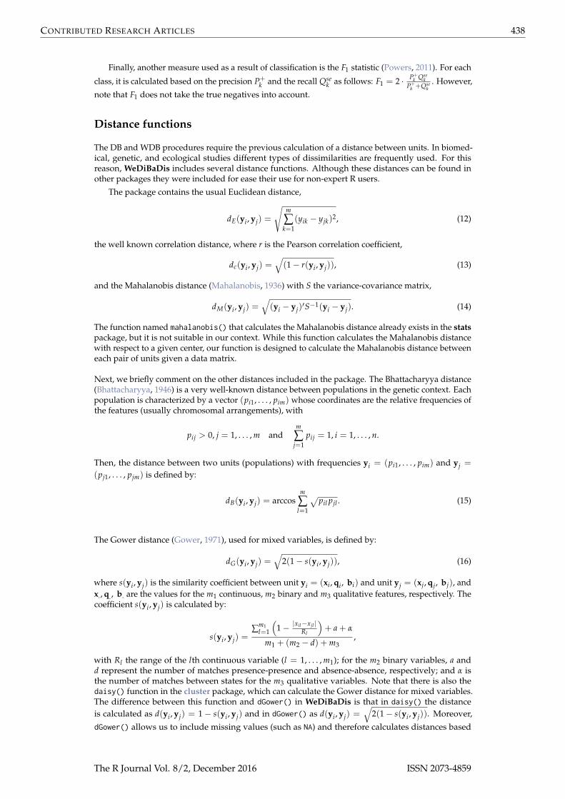
Figure 3: Plot of leave-one-out classification table for population genetics data in Example 2.

PredictedReal LA LE NLA NLELA 6 0 0 0LE 0 3 0 1NLA 0 0 13 0NLE 0 3 0 12

Total correct prediction: 89.47%Generalized squared correlation: 0.7442Cohen's Kappa coefficient: 0.8509804Sensitivity for each class:LA LE NLA NLE100.00 75.00 100.00 80.00Predictive value for each class:LA LE NLA NLE100.00 50.00 100.00 92.31Specificity for each class:LA LE NLA NLE87.50 91.18 84.00 95.65F1-score for each class:

LA LE NLA NLE100.00 60.00 100.00 85.71------ ------ ------ ------ ------ ------Prediction for new individuals:Pred. class1 "NLE"2 "NLA"

Now, the two unlabeled new units were correctly classified. The barplots are in Figure 3 and Figure 4,respectively.

Data files

The package contains some examples of data files, each with a corresponding explanation. Thedata sets are corearea, containing the data for the example presented in the subsection Example 1:Ecological data; abundances, which is a simulated data set for abundance data matrix; and microsatt,



1 2 3 4

020

4060

8010

0

SensitivityPositive predicted value

Specificity

Classes

Per

cent

age

Figure 4: Plot of the sensitivity, specificity, and positive predicted value for each class for populationgenetics data in Example 2.

a data set containing allele frequencies for 18 cattle breeds (bull or zebu), of French and African descent,typed on 9 microsatellites.

Computing time

To illustrate the time consumed by the WDB procedure, which requires more computation than DB, weperformed the following simulation with artificial data. We generated multinormal samples containing50, 100, 200, 300,. . . ,900, 1000, 2000, and 3000 units, respectively. Then, for each sample size we createdsets containing respectively 50, 100, 500, 1000, 1500, 2000, 2500, . . . , 4500, and 5000 features. For eachcombination of sample sizes and features, we considered 2, 3, 4, and 10 classes. All the computationspresented in this paper have been performed on a personal computer with Intel(R) Core(TM) i5-2450Mand 6 GB of memory using a single 2.50GHz CPU processor. The results of the simulation for twoclasses are displayed in Figure 5, where the elapsed time (the actual elapsed time since the processstarted) is reported in seconds. We can observe that the runtime is mainly affected by the numberof units (Figure 4, top), but affected very little by the number of variables (Figure 4, bottom). This isexpected, as the procedure is based on distances and therefore the dimension of the distance matrix(number of units) determines the runtime required. The number of classes also affects the runtime,although its variation with increasing the number of classes is very slight. For example, with 300 unitsand 4000 variables, the elapsed time for 2, 3, 4, and 10 classes are 3.38, 3.40, 3.62, and 4.82 seconds,respectively.

DB and WDB comparison using cancer data sets

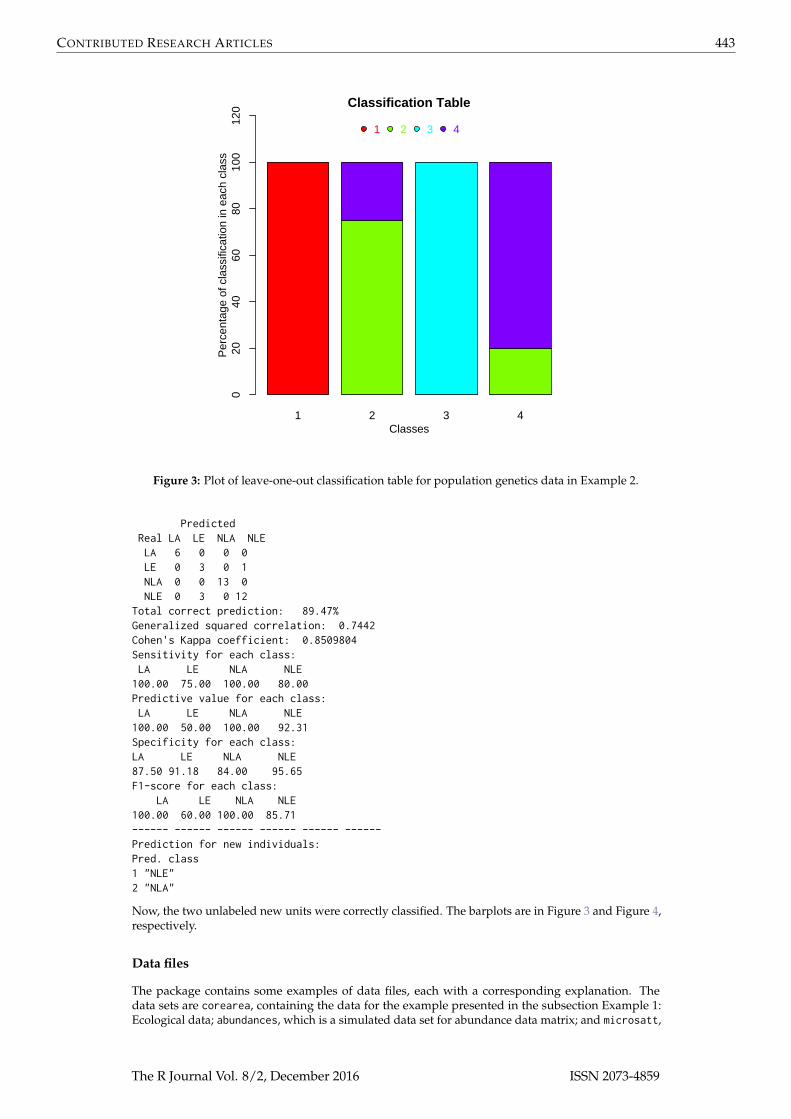
In order to compare the performance of DB and WDB procedures, thirty-eight available cancer datasets were considered in our analysis (Table 1). These are available at http://bioinformatics.rutgers.edu/Static/Supplements/CompCancer/datasets.htm and Lê Cao et al. (2010). As we can observe inTable 1, three of them include clinical features and some of the data sets have unbalanced classes. Weperformed the evaluation for DB and WDB classifiers using the leave-one-out procedure. We presentthe total misclassification rate MQt = 100− Qt and the generalized squared correlation coefficientGC2 (Table 2). For simplicity, the sensitivity Qkise, the specificity Qsp

k , the positive predictive value P+k

for each class, the Kappa and F1 statistcis are not presented. For the microarray data sets with onlycontinuous features we used the Euclidean distance, and for those including clinical and genetic data,


http://bioinformatics.rutgers.edu/Static/Supplements/CompCancer/datasets.htm

http://bioinformatics.rutgers.edu/Static/Supplements/CompCancer/datasets.htm


0

500

1000

1500

2000

2500

3000

0 500 1000 1500 2000 2500 3000

50

100

500

1000

1500

2000

2500

3000

3500

4000

4500

5000

0

500

11000

11500

2000

2500

0 1000 2000 3000 4000 5000 6000 7000 8000

50

100

200

300

400

500

600

700

800

900

1000

2000

3000

units

elap

sed

tim

ing

in s

eco

nd

s

features

elap

sed

tim

ing

in s

eco

nd

s

features

units

Figure 5: Artificial data sets with two classes. Top: Elapsed timing in seconds (y axes) for WDBprocedure with respect to the number of units (x axes). Each line (colours in the legend) correspondsto the set with identical number of features. Bottom: Elapsed timing in seconds (y axes) for WDBprocedure with respect to the number of features (x axes). Each line (colours in the legend) correspondsto the set with identical number of units.

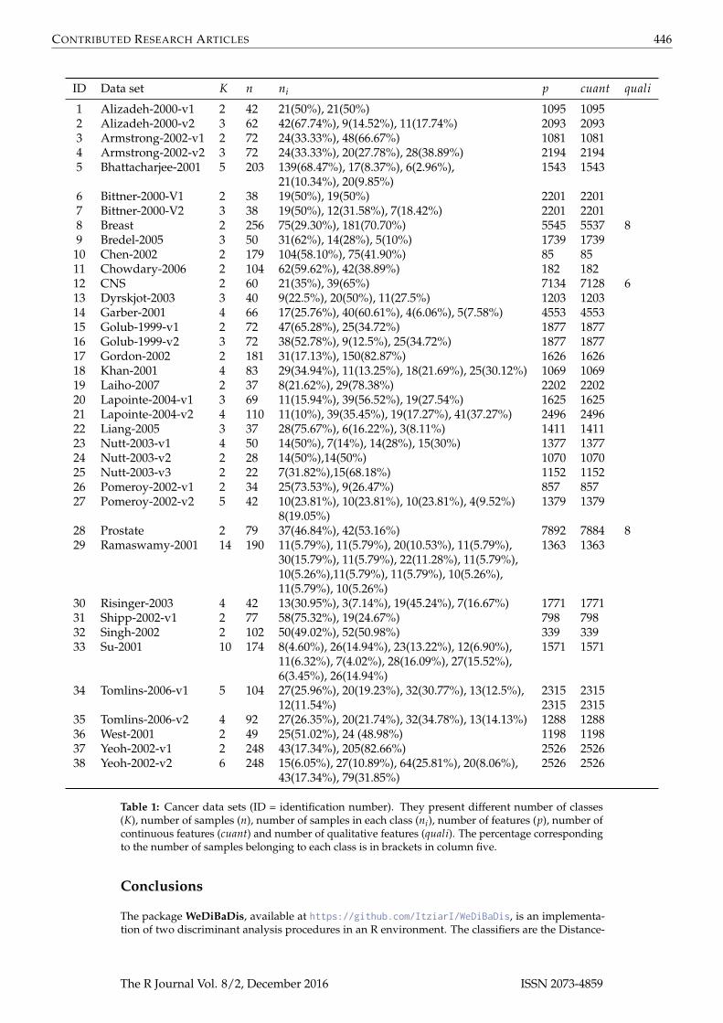
we considered the Gower distance (Gower, 1971). As we can observe in Table 2, considering only MQt,the total misclassification percentage rate, WDB was the best classifier in 18 data sets and it sharedthis quality in 11 data sets with DB (Wilcoxon signed rank test; one side p-value = 0.0265). Using thegeneralized squared correlation GC2 coefficient (Table 2), WDB was the best rule in 16 data sets andit shared this quality in 11 data sets with DB (Wilcoxon signed rank test; one side p-value = 0.0378).Note that for data sets 30 and 38 the GC2 value is 0. For example, in the Risinger-2003 case, all unitsof the second class (class with 3 units) were badly classified with DB and WDB methods. However,while with the DB method, 4 units belonging to other classes were badly classified in class 2, with theWDB method none of the units of other classes were badly classified in class 2, and for this reason theGC2 is equal to 0. With the Yeoh-2002-v2 data set something similar happened. For all these results,WDB seems to obtain in general the best results and to be a slightly better in the case where classes areunbalanced with respect to their sizes.



ID Data set K n ni p cuant quali

1 Alizadeh-2000-v1 2 42 21(50%), 21(50%) 1095 10952 Alizadeh-2000-v2 3 62 42(67.74%), 9(14.52%), 11(17.74%) 2093 20933 Armstrong-2002-v1 2 72 24(33.33%), 48(66.67%) 1081 10814 Armstrong-2002-v2 3 72 24(33.33%), 20(27.78%), 28(38.89%) 2194 21945 Bhattacharjee-2001 5 203 139(68.47%), 17(8.37%), 6(2.96%), 1543 1543

21(10.34%), 20(9.85%)6 Bittner-2000-V1 2 38 19(50%), 19(50%) 2201 22017 Bittner-2000-V2 3 38 19(50%), 12(31.58%), 7(18.42%) 2201 22018 Breast 2 256 75(29.30%), 181(70.70%) 5545 5537 89 Bredel-2005 3 50 31(62%), 14(28%), 5(10%) 1739 173910 Chen-2002 2 179 104(58.10%), 75(41.90%) 85 8511 Chowdary-2006 2 104 62(59.62%), 42(38.89%) 182 18212 CNS 2 60 21(35%), 39(65%) 7134 7128 613 Dyrskjot-2003 3 40 9(22.5%), 20(50%), 11(27.5%) 1203 120314 Garber-2001 4 66 17(25.76%), 40(60.61%), 4(6.06%), 5(7.58%) 4553 455315 Golub-1999-v1 2 72 47(65.28%), 25(34.72%) 1877 187716 Golub-1999-v2 3 72 38(52.78%), 9(12.5%), 25(34.72%) 1877 187717 Gordon-2002 2 181 31(17.13%), 150(82.87%) 1626 162618 Khan-2001 4 83 29(34.94%), 11(13.25%), 18(21.69%), 25(30.12%) 1069 106919 Laiho-2007 2 37 8(21.62%), 29(78.38%) 2202 220220 Lapointe-2004-v1 3 69 11(15.94%), 39(56.52%), 19(27.54%) 1625 162521 Lapointe-2004-v2 4 110 11(10%), 39(35.45%), 19(17.27%), 41(37.27%) 2496 249622 Liang-2005 3 37 28(75.67%), 6(16.22%), 3(8.11%) 1411 141123 Nutt-2003-v1 4 50 14(50%), 7(14%), 14(28%), 15(30%) 1377 137724 Nutt-2003-v2 2 28 14(50%),14(50%) 1070 107025 Nutt-2003-v3 2 22 7(31.82%),15(68.18%) 1152 115226 Pomeroy-2002-v1 2 34 25(73.53%), 9(26.47%) 857 85727 Pomeroy-2002-v2 5 42 10(23.81%), 10(23.81%), 10(23.81%), 4(9.52%) 1379 1379

8(19.05%)28 Prostate 2 79 37(46.84%), 42(53.16%) 7892 7884 829 Ramaswamy-2001 14 190 11(5.79%), 11(5.79%), 20(10.53%), 11(5.79%), 1363 1363

30(15.79%), 11(5.79%), 22(11.28%), 11(5.79%),10(5.26%),11(5.79%), 11(5.79%), 10(5.26%),11(5.79%), 10(5.26%)

30 Risinger-2003 4 42 13(30.95%), 3(7.14%), 19(45.24%), 7(16.67%) 1771 177131 Shipp-2002-v1 2 77 58(75.32%), 19(24.67%) 798 79832 Singh-2002 2 102 50(49.02%), 52(50.98%) 339 33933 Su-2001 10 174 8(4.60%), 26(14.94%), 23(13.22%), 12(6.90%), 1571 1571

11(6.32%), 7(4.02%), 28(16.09%), 27(15.52%),6(3.45%), 26(14.94%)

34 Tomlins-2006-v1 5 104 27(25.96%), 20(19.23%), 32(30.77%), 13(12.5%), 2315 231512(11.54%) 2315 2315

35 Tomlins-2006-v2 4 92 27(26.35%), 20(21.74%), 32(34.78%), 13(14.13%) 1288 128836 West-2001 2 49 25(51.02%), 24 (48.98%) 1198 119837 Yeoh-2002-v1 2 248 43(17.34%), 205(82.66%) 2526 252638 Yeoh-2002-v2 6 248 15(6.05%), 27(10.89%), 64(25.81%), 20(8.06%), 2526 2526

43(17.34%), 79(31.85%)

Table 1: Cancer data sets (ID = identification number). They present different number of classes(K), number of samples (n), number of samples in each class (ni), number of features (p), number ofcontinuous features (cuant) and number of qualitative features (quali). The percentage correspondingto the number of samples belonging to each class is in brackets in column five.

Conclusions

The package WeDiBaDis, available at https://github.com/ItziarI/WeDiBaDis, is an implementa-tion of two discriminant analysis procedures in an R environment. The classifiers are the Distance-


https://github.com/ItziarI/WeDiBaDis


ID 100−Qt 100−Qt GC2 GC2

DB WDB DB WDB

1 7.14 7.14 0.74 0.742 1.61 0.00 0.94 1.003 8.33 5.56 0.684 0.774 4.17 4.17 0.88 0.885 19.21 15.27 0.49 0.566 13.16 13.16 0.56 0.567 36.84 36.84 0.25 0.258 32.81 30.47 0.11 0.139 18.00 18.00 0.34 0.34

10 11.17 8.94 0.61 0.6711 18.27 9.62 0.42 0.6412 41.67 38.33 0.01 0.0113 15.00 12.50 0.58 0.6514 21.21 28.79 0.38 0.1915 6.94 4.17 0.72 0.8216 6.94 6.94 0.81 0.8117 12.71 13.26 0.47 0.4218 1.20 1.20 0.97 0.9719 21.62 21.62 0.23 0.2320 31.88 30.43 0.23 0.2621 30.91 30.91 0.34 0.3422 13.51 10.81 0.72 0.7623 32.00 34.00 0.40 0.3324 17.86 10.71 0.43 0.6525 4.55 9.09 0.80 0.6726 29.41 20.59 0.12 0.1627 16.67 21.43 0.65 0.6328 34.18 34.18 0.10 0.1029 36.84 29.47 0.44 0.5330 28.57 26.19 0.36 0.0031 29.87 12.99 0.24 0.4832 30.39 30.39 0.18 0.1633 20.11 16.67 0.63 0.7034 17.31 21.15 0.66 0.5835 23.91 26.09 0.46 0.4136 20.41 14.29 0.35 0.5237 1.61 2.02 0.89 0.8738 21.77 24.60 0.57 0.00

Table 2: In the first column identification number for cancer data sets. In the second and thirdcolumns, total leave-one-out misclassification rate 100−Qt (in percentage) for classifiers DB and WDB,respectively. In bold the smallest misclassification rate. In the forth and fifth columns, generalizedsquared correlation GC2 coefficient for classifiers DB and WDB, respectively. In bold the greater GC2

value.

Based (DB) and the new proposed procedure Weighted-Distance-Based (WDB). Thee are useful tosolve the classification problem for high-dimensional data sets with mixed features or when the inputinformation is a distance matrix. This software provides functions to compute both discriminantprocedures and to assess the performance of the classification rules it offers: the leave-one-out classifi-cation table; the general correlation coefficient; the sensitivity, specificity, and positive predictive valuefor each class; the Kappa and the F1 statistics. The package also presents these results in a graphicalform (barplots for the classification table and, for sensitivity, specificity and positive predictive values,respectively). Furthermore, it allows the classification for new unlabeled units. WeDiBaDis providesa user-friendly environment, which can be of great utility in biology, ecology, biomedical, and, in gen-eral, any applied study involving discrimination between groups and classification of new unlabeledunits. In addition, it can be very useful in multivariate methods courses aimed at biologists, medicalresearchers, psychologists, etc.



Acknowledgements

This research was partially supported: II by the Spanish ‘Ministerio de Economia y Competitividad’(TIN2015-64395-R) and by the Basque Government Research Team Grant (IT313-10) SAIOTEK ProjectSA-2013/00397 and by the University of the Basque Country UPV/EHU (Grant UFI11/45 (BAILab).FM by the Spanish ‘Ministerio de Economia y Competitividad’ (CTM2013-48163) and by Grant 2014SGR 336 from the Departament d’Economia i Coneixement de la Generalitat de Catalunya. CA by theSpanish ‘Ministerio de Economia y Competitividad’ (SAF2015-68341-R), by the Spanish ‘Ministeriode Economia y Competitividad’ (TIN2015-64395-R) and by Grant 2014 SGR 464 (GRBIO) from theDepartament d’Economia i Coneixement de la Generalitat de Catalunya.

Bibliography

M. J. Anderson and J. Robinson. Generalized discriminant analysis based on distances. Australian andNew Zealand Journal of Statistics, 45:301–318, 2003. [p435]

I. Balanyà, E. Solé, J. M. Oller, D. Sperlich, and L. Serra. Long-term changes in chromosomal inversionpolymorphism of Drosophila subobscura: II. European populations. Journal of Zoological Systematicsand Evolutionary Research, 42:191–201, 2004. [p442]

P. Baldi, S. Brunak, Y. Chauvin, C. A. F. Andersen, and H. Nielsen. Assessing the accuracy of predictionalgorithms for classification: An overview. Bioinformatics, 16:412–424, 2000. [p437]

A. Bhattacharyya. On a measure of divergence of two multinominal populations. Sankhya, 7:401–406,1946. [p438]

R. Blagus and L. Lusa. Improved shrunken centroid classifiers for high-dimensional class-imbalanceddata. BMC Bioinformatics, 14:64, 2013. [p435]

G. Bouin. Computer program review: Ginkgo, a multivariate analysis package. Journal of VegetationScience, 16:355–359, 2005. [p435]

A. L. Boulesteix, C. Porzelius, and M. Daumer. Microarray-based classification and clinical predictors:On combined classifiers and additional predictive value. Bioinformatics, 24:1698–1706, 2008. [p434]

J. R. Bray and J. T. Curtis. An ordination of upland forest communities of southern Wisconsin. EcologicalMonographs, 27:325–349, 1957. [p439]

L. Breiman. Random forests. Machine Learning, 45:5–32, 2001. [p434]

J. Cohen. A coefficient of agreement for nominal scales. Educational and Psychological Measurement, 20:37–46, 1960. [p437]

T. M. Cover and P. E. Hart. Nearest neighbor pattern classification. IEEE Transactions on InformationTheory, 13:21–27, 1967. [p435]

C. M. Cuadras. Statistical Data Analysis and Inference, chapter Distance Analysis. In: Discrimination andClassfication Using Both Continuous and Categorical Variables, pages 459–473. Elsevier SciencePublishers BV, Amsterdam, 1989. [p435]

C. M. Cuadras. Some examples of distance based discrimination. Biometrical Letters, 29:3–20, 1992.[p435]

C. M. Cuadras, J. Fortiana, and F. Oliva. The proximity of an individual to a population withapplications in discriminant analysis. Journal of Classification, 14:117–136, 1997. [p435, 436]

M. De Caceres, F. Oliva, and X. Font. GINKGO, a multivariate analysis program oriented towardsdistance-based classifications. In International Conference on Correspondence Analysis and RelatedMethods (CARME’ 03), 2003. [p435]

R. O. Duda, P. E. Hart, and D. G. Stork. Pattern Classification. Wiley Interscience Publication. JohnWiley and Sons, New York, 2000. [p435]

S. Dudoit, J. Fridlyand, and T. P. Speed. Comparison of discrimination methods for the classification oftumors using gene expression data. Journal of American Statistical Association, 97:77–87, 2002. [p434]

A. H. Fielding. Cluster and Classification Techniques for the Biosciences. Cambridge University Press, 2007.[p440]



R. A. Fisher. The use of multiple measurements in taxonomic problems. The Annals of Eugenics, 7:179–188, 1936. [p434]

A. K. Ghosh and P. Chaudhuri. On data depth and distribution-free discriminant analysis usingseparating surfaces. Bernoulli, 11:1–27, 2005. [p435]

T. R. Golub, D. K. Slonim, P. Tamayo, C. Huard, M. Gaasenbeek, J. P. Mesirov, H. Coller, M. L. Loh, J. R.Downing, M. A. Caligiuri, and C. D. Bloomfield. Molecular classification of cancer: Class discoveryand class prediction by gene expression monitoring. Science, 286:531–537, 1999. [p434]

J. C. Gower. A general coefficient of similarity and some of its properties. Biometrics, 27:857–871, 1971.[p438, 445]

T. Hastie, R. Tibshirani, D. Botstein, and P. Brown. Supervised harvesting of expression trees. GenomeBiology, 2:1–12, 2001. [p434]

D. Hlubinka and O. Vencalek. Depth-based classification for distributions with nonconvex support.Journal of Probability and Statistics, 28:1–7, 2013. [p435]

I. Irigoien, F. Mestres, and C. Arenas. The depth problem: Identifying the most representative units ina data group. IEEE/ACM Transactions on Computational Biology and Bioinformatics, 10:161–172, 2013a.[p435, 436]

I. Irigoien, B. Sierra, and C. Arenas. ICGE: An R package for detecting relevant clusters and atypicalunits in gene expression. BMC Bioinformatics, 13:30–41, 2013b. [p439]

J. Jin and H. Cui. Discriminant analysis based on statistical depth. Journal of Systems Science andComplexity, 23:362–371, 2010. [p435]

R. Jornstein. Clustering and classification based on L1 data depth. Journal of Multivariate Analysis, 90:67–89, 2004. [p435]

M. Kent. Vegetation Description and Data Analysis: A Practical Approach. Wiley-Blackwey, 2011. [p435]

W. I. Krzanowski, P. Jonathan, W. V. McCarthy, and M. R. Thomas. Discriminant analysis with singularcovariance matrices: Methods and applications to spectroscopic data. Applied Statistics, 44:101–115,1995. [p434]

J. R. Landis and G. G. Koch. The measurement of observer agreement for categorical data. Biometrics,33:159–174, 1977. [p437]

K. A. Lê Cao, E. Meugnier, and G. J. McLachlan. Integrative mixture of experts to combine clinicalfactors and gene markers. Bioinformatics, 26:1192–1198, 2010. [p444]

P. Legendre and L. Legendre. Numerical Ecology. Elsevier, Amsterdam, 1998. [p435]

R. Y. Liu. On a notion of data depth based on random simplices. Annals of Statistics, 18:405–414, 1990.[p435]

P. V. Mahalanobis. On the generalized distance in statistics. Procedures of the Natural Institute of Scienceof India, 2:49–55, 1936. [p438]

B. W. Matthews. Comparison of the predicted and observed secondary structure of t4 phage lysozyme.Biochimica Biophysica Acta, 405:442–451, 1975. [p437]

F. Mestres, J. Balanyà, M. Pascual, C. Arenas, G. W. Gilchrist, R. B. Huey, and L. Serra. Evolutionof Chilean colonizing populations of D. subobscura: lethal genes and chromosomal arrangements.Genetica, 136:37–48, 2009. [p442]

L. Orloci. An agglomerative method for classification of plant communities. Journal of Ecology, 55:193–205, 1967. [p435, 439]

D. M. W. Powers. Evaluation: From precision, recall and F-measure to ROC, informedness, markednessand correlaction. Journal of Machine Learning Technologies, 2:37–63, 2011. [p438]

A. Prevosti, J. Ocaña, and G. Alonso. Distances between populations of D. subobscura, based onchromosome arrangement frequencies. Theoretical and Applied Genetics, 45:231–241, 1975. [p439]

C. R. Rao. A review of canonical coordinates and an alternative to correspondence analysis usingHellinger distance. Qüestiió, 19:23–63, 1995. [p439]



R. Serfling. Statistic and Data Analysis Based on L1-Norm and Related Methods, chapter A Depth Functionand a Scale Curve Based on Spatial Quantiles, pages 25–38. Birkhäuser, Boston, 2002. [p435]

E. Solé, F. Mestres, J. Balanyà, C. Arenas, and L. Serra. Colonization of America by D. subobscura:Spatial and temporal lethal-gene allelism. Hereditas, 133:65–72, 2000. [p442]

R. Tibshirani, T. Hastie, B. Narasimhan, and G. Chu. Diagnosis of multiple cancer types by shrunkencentroids of gene expression. Proceedings of the National Academy of Sciences of the United States ofAmerica, 99:6567–6572, 2002. [p434]

Y. Vardi and C. Zhang. The multivariate L1-median and associated data depth. Proceedings of theNational Academy of Sciences of the United States of America, 97:1423–1426, 2000. [p435]

X. H. Zhou, N. A. Obuchowski, and D. K. McClish. Statistical Methods in Diagnostic Medicine. WileySeries in Probability and Statistics. John Wiley and Sons, New Jersey, 2002. [p437]

S. Zuo and R. Serfling. General notions of statistical depth function. Annals of Statistics, 28:461–482,2000. [p435, 436]

Itziar IrigoienDepartment of Computation Science and Artificial IntelligenceUniversity of the Basque Country UPV/EHUDonostia, [email protected]

Francesc MestresDepartment of Genetics, Microbiology and Statistics. Genetics SectionUniversity of BarcelonaBarcelona, [email protected]

Concepcion ArenasDepartment of Genetics, Microbiology and Statistics. Statistics SectionUniversity of BarcelonaBarcelona, [email protected]


mailto:[email protected]



weighted distance based discriminant analysis: the r ... · pdf fileweighted distance based...

Documents