Weighted Mat hings in General Graphs

Diplomarbeit von Guido S h�afer

Diese Arbeit wurde unter der Betreuung von Prof. Dr. Kurt Mehlhorn am Max{Plan k{Institut f�ur Informatik in Saarbr�u ken innerhalb der Fa hri htung 6.2, Informatik, derUniversit�at des Saarlandes angefertigt.

Hiermit erkl�are i h an Eides Statt, da� i h diese Diplomarbeit selbst�andig verfa�t undnur die im Literaturverzei hnis angegebenen Quellen benutzt habe. Ferner habe i h dieArbeit no h keinem anderen Pr�ufungsamt vorgelegt.Saarbr�u ken, 31. Mai 2000

An dieser Stelle m�o hte i h mi h bei Prof. Dr. Kurt Mehlhorn f�ur die Vergabe des sehrinteressanten Themas und die ausgezei hnete Betreuung sowie f�ur die Bereitstellung derhervorragenden Arbeitsbedingungen amMax{Plan k{Institut f�ur Informatik bedanken.Ferner m�o hte i h all jenen danken, die dur h ihre Hilfe ma�gebli h zum Gelingendieser Arbeit beigetragen haben, insbesondere Jo hen K�onemann und Robert Spen ef�ur das Korrekturlesen. Ein gro�er Dank gilt meinen Freunden, die mi h die ganze Zeit�uber und besonders in der Endphase immer wieder unterst�utzten. Letztli h m�o htei h meinen Eltern danken, die mir das Studium erm�ogli hten und besonders meinerFreundin Sabine, die immer f�ur mi h da war.

ContentsIntrodu tion 11 Mat hing Theory 51.1 The Mat hing Problem and its Variants . . . . . . . . . . . . . . . . . . 51.2 Mat hing Con epts . . . . . . . . . . . . . . . . . . . . . . . . . . . . . . 71.3 Edmonds' Blossom{Shrinking Approa h . . . . . . . . . . . . . . . . . . 101.4 LP Formulations for Weighted Mat hing Problems . . . . . . . . . . . . 181.4.1 LP Formulation for the Weighted Mat hing Problem . . . . . . . 181.4.2 LP Formulation for the Weighted Perfe t Mat hing Problem . . 201.4.3 An Alternative LP Formulation for the Weighted Perfe t Mat h-ing Problem . . . . . . . . . . . . . . . . . . . . . . . . . . . . . . 211.5 Redu tions . . . . . . . . . . . . . . . . . . . . . . . . . . . . . . . . . . 221.5.1 Redu ing the Weighted Mat hing Problem to the Weighted Per-fe t Mat hing Problem . . . . . . . . . . . . . . . . . . . . . . . . 221.5.2 Redu ing the Weighted Perfe t Mat hing Problem to theWeighted Mat hing Problem . . . . . . . . . . . . . . . . . . . . 231.6 Primal{Dual Method . . . . . . . . . . . . . . . . . . . . . . . . . . . . . 241.6.1 Primal{Dual Method for the Maximum{Weight Mat hing Problem 251.6.2 Di�eren es in Weighted Perfe t Mat hing Case . . . . . . . . . . 271.6.3 The Blossom{Shrinking Approa h Revisited . . . . . . . . . . . . 281.6.4 Half{Integrality of the Dual Solution . . . . . . . . . . . . . . . . 341.6.5 Using the Alternative LP Formulation |Algorithmi Consequen es 351.7 Survey of Di�erent Realizations . . . . . . . . . . . . . . . . . . . . . . . 361.7.1 An O(n2m) Approa h . . . . . . . . . . . . . . . . . . . . . . . . 371.7.2 An O(n3) Approa h . . . . . . . . . . . . . . . . . . . . . . . . . 37I

II Contents1.7.3 An O(nm logn) Approa h . . . . . . . . . . . . . . . . . . . . . . 381.7.4 An O(n(m+ n logn)) Approa h . . . . . . . . . . . . . . . . . . 392 O(nm logn) Approa h 412.1 Varying Potentials and Redu ed Costs . . . . . . . . . . . . . . . . . . . 412.1.1 Potential Update . . . . . . . . . . . . . . . . . . . . . . . . . . . 422.1.2 Maintenan e of Redu ed Costs . . . . . . . . . . . . . . . . . . . 432.1.3 Managing the Blossom O�sets . . . . . . . . . . . . . . . . . . . 442.2 Determination of Æ | towards a Priority Queue Approa h . . . . . . . . 472.3 A Misleading Strategy | Traps and Pitfalls . . . . . . . . . . . . . . . . 492.3.1 Maximum Height of a Blossom Tree . . . . . . . . . . . . . . . . 502.3.2 Expanding a Blossom | Number of Status Changes . . . . . . . 522.4 Con atenable Priority Queues . . . . . . . . . . . . . . . . . . . . . . . . 533 Implementation and Tests 573.1 Fun tionality . . . . . . . . . . . . . . . . . . . . . . . . . . . . . . . . . 583.2 Con atenable Priority Queues ( on at pq ) . . . . . . . . . . . . . . . . 613.3 Single Sear h Tree Approa h . . . . . . . . . . . . . . . . . . . . . . . . 633.3.1 Data Stru tures . . . . . . . . . . . . . . . . . . . . . . . . . . . . 633.3.2 Algorithm . . . . . . . . . . . . . . . . . . . . . . . . . . . . . . . 673.4 Multiple Sear h Tree Approa h . . . . . . . . . . . . . . . . . . . . . . . 903.4.1 Data Stru tures . . . . . . . . . . . . . . . . . . . . . . . . . . . . 923.4.2 Algorithm . . . . . . . . . . . . . . . . . . . . . . . . . . . . . . . 973.5 Constru ting Better Initial Solutions . . . . . . . . . . . . . . . . . . . . 1153.5.1 Greedy Heuristi . . . . . . . . . . . . . . . . . . . . . . . . . . . 1163.5.2 Fra tional Mat hing Problem . . . . . . . . . . . . . . . . . . . . 1183.6 Experimental Results . . . . . . . . . . . . . . . . . . . . . . . . . . . . . 130Open Problems 141Bibliography 143

Introdu tionCombinatorial optimization is a �eld of applied mathemati s and theoreti al omputers ien e. A major topi in ombinatorial optimization are linear optimization problems.Said simply, a linear optimization problem requires the optimization of a linear fun -tion over a dis rete set of solutions. An intensively studied and well{known problemin ombinatorial optimization is the weighted mat hing problem: it requires the om-putation of a mat hing having maximum or minimum weight. A mat hing M in anundire ted graph G is a set of edges no two of whi h share an endpoint. The edges ofG are asso iated with weights and the total weight of a mat hing M is the sum of allthe weights of the edges in M . M may further be restri ted to being perfe t, whi h onstitutes the weighted perfe t mat hing problem; a mat hing M is perfe t, if everyvertex in G has exa tly one in ident edge in M .Many variants and extensions of the weighted mat hing problem exist. As an exampleof a variant, G might be restri ted to being bipartite; this is alled the bipartite weightedmat hing problem. An example of an extension, on the other hand, is the b{mat hingproblem, where ea h vertex may have up to b in ident mat hing edges.There are (at least) three types of appli ations that motivate the investigation ofweighted mat hing problems. (1) Dire t appli ations of the weighted mat hing prob-lem exist. (2) Many other problems an be redu ed to the weighted mat hing problem.(3) Several algorithms (repeatedly) solve the weighted mat hing problem in order toprogress. We will give examples of ea h of the three appli ation types stated. Someof these are widely known. Additionally, we wish to present two new appli ations (oftype (2) and (3)) that were en ountered during the writing of the thesis and thus havebeen, for us, a major sour e of motivation.A lassi example of an appli ation of type (1) is to optimize, i.e. in this ase to mini-mize, the time spent by a plotter pen in pen{up motion, i.e. moving from one point toanother without drawing. Reingold and Tarjan [RT81℄ showed this to be a weightedperfe t mat hing problem. We brie y summarize their reasoning. Assume we wish toplot a onne ted �gure, and assume further that the time spent by the plotter movingfrom one point to another is proportional to the Eu lidean distan e. We lassify thestarting and rossing points of the �gure (i.e. the points where a line starts or severallines ross) to be either odd or even. A point is odd when an odd number of linesemerge, otherwise it is even. A fundamental theorem in graph theory is that thereexists always an even number of odd points. Moreover, Euler proved that a �gure an be tra ed (starting and ending in the same point) with no pen{up motion i� it is onne ted and no odd points exist. Thus, we need to �nd a new set of lines su h thatea h odd point be omes even and, moreover, the total time of pen{up motion along1

2 Introdu tionthese lines is minimized. We thus de�ne a omplete graph G whose verti es orrespondto the odd points of the �gure and whose edge weights orrespond to the Eu lideandistan e of these points. Minimizing the time of pen{up motion then means �nding aminimum{weight perfe t mat hing in G.An example of type (2), whi h we would like to present as a motivating appli ation forthe weighted mat hing problem, is the so{ alled dominan e problem. Its appli ationstems from the �eld of omputational linguisti s. A dominan e problem is given by a olle tion of vertex disjoint rooted trees and a set of dominan e wishes. A dominan ewish is a dire ted edge from a leaf of some tree to the root of some other tree | theleaf wishes to dominate the root. The task is to assemble the trees into a forest su hthat every dominan e wish is satis�ed, i.e. ea h dire ted edge redu es to an an estor{prede essor relationship. Althaus et al. [ADK+00℄ re ently showed that de iding thesatis�ability of a dominan e problem an be redu ed to a weighted mat hing problem.As an example of type (3), we onsider a fundamental ommuni ation problem knownas gossiping: n pro essing units are required to inter hange their data with ea h other.The underlying ommuni ation network is modeled by a graph G. A pro essing unit(i.e. vertex) is permitted to ommuni ate with only one of its neighbours (i.e. adja entverti es) at a time. The task of stating an optimal gossiping s hedule, su h that inthe end every pro essing unit knows the data of all other pro essing units, is NP{hard.Beier and Sibeyn [BS00℄ use a mat hing heuristi to ompute a good, sub{optimal gos-siping s hedule. The heuristi an be regarded as working in rounds. In ea h round,weights are assigned (on the basis of di�erent riteria) to the onne tions (i.e. edges)of the ommuni ation network. Then, a maximum{weight mat hing is omputed withrespe t to these weights. The pairs of mat hed pro essing units ommuni ate withea h other. Another well{known example of this type is Christo�des' approximationalgorithm for the traveling salesman problem (see [Chr76℄). The problem is de�ned bya omplete graph G onsisting of n verti es (whi h represent ities), where the edgeweights orrespond to the Eu lidean distan es. The task is to �nd a tour of minimumlength. Christo�des' algorithm omputes a tour whose length is at most 3/2 as longas the length of an optimum tour; it is still the urrently best known approximationalgorithm for the traveling salesman problem. In a �rst step, the algorithm onstru tsa minimum spanning tree T of G, and afterwards a minimum{weight perfe t mat hingM on the odd degree verti es of T is omputed. The graph T [M then redu es to atour with the desired property.Various other examples of the above{mentioned appli ation types exist and an befound, for example, in Ball, Bodin and Dial [BBD83℄, Derigs and Metz [DM92℄, Bell[Bel94℄ and Ahuja, Magnanti and Orlin [AMO93℄.Mat hing problems have been the subje t of intensive resear h over several de ades.The earliest result in mat hing theory we ame a ross, widely known as K�onig's The-orem, dates ba k to 1916 (see [K�on16℄). One of the ornerstones in mat hing theoryis due to Edmonds [Edm65b, Edm65a℄. In 1965, he invented the famous blossom{shrinking algorithm, whi h enables a solution for the weighted mat hing problem tobe omputed in polynomial{time. A straightforward implementation, as originallyproposed by Edmonds himself, requires time O(n2m), where n and m denote thenumber of verti es and edges in G, respe tively. Sin e then, the theoreti al running{time of the blossom{shrinking approa h has been su essively improved. Both Lawler[Law76℄ and Gabow [Gab74℄ improved the asymptoti running{time to O(n3). Later,

Introdu tion 3Galil, Mi ali and Gabow [GMG86℄ a hieved O(nm logn) and �nally Gabow [Gab90℄stated that Edmonds' blossom{shrinking algorithm an be implemented to run in timeO(n(m+n logn)). Somewhat better asymptoti time bounds an be a hieved for integeredge weights using s aling algorithms (see Gabow and Tarjan [GT91℄).The urrently most eÆ ient odes implement variants of Edmonds' blossom{shrinkingalgorithm and are based on either the O(n2m) or O(n3) approa h. For the time being,the best known implementation, named Blossom IV, is due to Cook and Rohe [CR97℄.Their implementation is based on earlier work by Applegate and Cook [App93℄. Theydo not laim a theoreti al time bound, but, as we shall see, it annot be better than(n3). Blossom IV is known to be highly eÆ ient in pra ti e; the data stru tures ituses are simple.The algorithms suggested by Galil, Mi ali and Gabow [GMG86℄ and by Gabow [Gab90℄mainly a hieve a better asymptoti time bound by using sophisti ated data stru tures.For example, the algorithm of Galil, Mi ali and Gabow requires a data stru ture on- atenable priority queue, in whi h the priorities of ertain subgroups of verti es an beuniformly hanged by a single operation. Up to now, it has been an open question (andone expli itly posed in [App93℄ and [CR97℄), whether or not the use of sophisti ateddata stru tures will help in pra ti e. We will answer this question in the aÆrmative:the implementation we shall present in this thesis is based on the ideas of Galil, Mi aliand Gabow and turned out to be ompetitive | if not even superior | to Blossom IV.The stru ture of the thesis is as follows. In Chapter 1, we will develop all details ofthe blossom{shrinking algorithm. We will start with the de�nition of some variants ofthe weighted mat hing problem and introdu e important on epts, su h as augmentingpaths, that are ru ial to almost all mat hing algorithms. The blossom{shrinking ap-proa h will �rst be onsidered for the ardinality mat hing ase. Linear programmingformulations for both the weighted mat hing problem and the weighted perfe t mat h-ing problem will then be investigated. Duality theory will lead us towards a primal{dualmethod for the weighted mat hing problem based on Edmonds' blossom{shrinking ap-proa h. Finally, we will on lude the hapter with a brief survey of the four di�erentrealizations mentioned above.In Chapter 2, we will illustrate the ideas underlying our implementation. Most ofthese are based on or have been developed from the ideas put forward by Galil, Mi aliand Gabow [GMG86℄. We will outline how the blossom{shrinking approa h an beimplemented using priority queues. The diÆ ulty of handling varying priorities withinthese priority queues will be over ome by taking advantage of the fa t that these values hange uniformly. Moreover, we will demonstrate in detail the need for on atenablepriority queues.In Chapter 3 we will des ribe our implementation and dis uss some experimental re-sults. We implemented two versions of the algorithm: a single sear h tree approa h anda multiple sear h tree approa h. First, the results from Chapter 2 will be in orporatedinto a single sear h tree algorithm. Then, all ne essary extensions and modi� ations forthe multiple sear h tree approa h will be presented. The eÆ ien y of both algorithmsis onsiderably improved by using a heuristi to reate a better initial solution. We willdis uss two heuristi s: a greedy heuristi and a fra tional mat hing heuristi . Finally,some running{time experiments will reveal the eÆ ien y of our algorithms in pra ti e.

Chapter 1Mat hing TheoryIn this hapter we will establish essential on epts that are fundamental for later dis- ussion. We begin with the de�nition of the mat hing problem and outline some of itsvariants. Some useful notations su h as the on ept of augmenting paths will followand lead to a �rst generi algorithm solving mat hing problems. Starting with the ardinality mat hing problem, we will present the main ideas of Edmonds' well{knownblossom{shrinking approa h. Results from the �eld of ombinatorial optimization willguide us towards an extension of the blossom{shrinking approa h for weighted mat hingproblems.1.1 The Mat hing Problem and its VariantsLet G = (V;E) be an undire ted graph, where V and E denote the set of verti es andedges, respe tively. The number of verti es and edges are referred to by n = jV j andm = jEj. Sin e G is undire ted, we will denote an edge e between two verti es u and vas an unordered pair fu; vg, or uv for short. G is bipartite when a partition V = A _[Bof the verti es of G exists and ea h edge uv 2 E has exa tly one vertex in A and onein B.An ordered sequen e p = (e1; e2; : : : ; ek) of edges, with ei = uiui+1 2 E, 1 � i � k, is alled a path from u1 to uk+1 in G. Alternatively, we will represent p by the sequen ep = (u0; u1; : : : ; uk) of verti es traversed. A path p is alled simple, when all verti eson p are distin t. Let C be a path starting and ending with the same vertex. C isthen alled a y le. Moreover, C is said to be a simple y le, when no other y le is ontained in C.A mat hing M of G is a subset of edges su h that no two edges of M share a ommonvertex (see Figure 1.1 for an example). All edges inM are said to be mat hed and edgesin the di�eren e E nM are unmat hed. Analogously, a vertex u is said to be mat hed ifthere exists an in ident mat hed edge uv 2 M ; otherwise u is unmat hed or free. Theadja ent vertex v of u with respe t to a mat hed edge e = uv is the mate of u. M is aperfe t mat hing when all verti es of G are mat hed and hen e jM j = n=2.The mat hing problem is to �nd a mat hing in a graph G that meets ertain require-5

6 Chapter 1. Mat hing Theorya b

g h d efFigure 1.1: Let G be the graph depi ted above. M = fag; h; dfg is a mat hing of G.p = (e; f; d) is an example of an alternating path. p0 = (b; h; ; d; f; e) is an augmenting path.M 0 =M �p0 = fag; bh; d; feg is a mat hing in G with jM 0j = jM j+1. M 0 is perfe t and hen ea maximum{ ardinality mat hing of G.ments. We will distinguish between two kinds of mat hing problems: the unweightedand the weighted mat hing problem. In the weighted mat hing problem a weight fun -tion w : E 7�! R on the edges of G is additionally given. The distin tion is furtherre�ned on the basis of whether or not G is bipartite. Altogether we lassify four variantsof the mat hing problem, whi h are de�ned below.Maximum{Cardinality Bipartite Mat hing Let G = (A _[B;E) be a bipartitegraph. The maximum{ ardinality bipartite mat hing problem is to �nd a mat hing Min G of maximum ardinality, i.e. jM j � jM 0j for any other mat hing M 0 of G.Maximum{Cardinality Mat hing Consider a general graph G = (V;E). In themaximum{ ardinality mat hing problem a mat hing M of maximum ardinality has tobe determined.In both ardinality ases, M need not ne essarily be perfe t. However, every perfe tmat hing of G forms a maximum{ ardinality mat hing.Maximum{Weight Bipartite Mat hing Let G = (A _[B;E;w) be a bipartitegraph with weight fun tion w. Finding a mat hing M with total weight w(M) =Pe2M w(e) and w(M) � w(M 0) for all other mat hings M 0 of G onstitutes themaximum{weight bipartite mat hing problem.In the maximum{weight bipartite perfe t mat hing problem M is further restri ted tobeing perfe t. This problem is also known as the maximum{weight assignment problem.Maximum{Weight Mat hing The most general ase of all mat hing problems isthe maximum{weight mat hing problem. Given a general graph G = (V;E;w) with

1.2 Mat hing Con epts 7weight fun tion w, the task is to �nd a mat hing M having maximum weight w(M)among all possible mat hings of G.As above, one might wish to obtain a perfe t mat hing of maximum weight. This onstitutes the maximum{weight perfe t mat hing problem.Let G = (V;E;w) be an instan e of a weighted mat hing problem. One might wishto obtain a mat hing of minimum instead of maximum weight in G. However, ea hminimum{weight mat hing problem an be redu ed to an appropriate maximum{weightmat hing problem by negating the signs of all weights. That is, a maximum{weightmat hing M of G0 = (V;E;�w) will be a mimimum{weight mat hing in G.Many other variants and extensions of the mat hing problem exist; for example f{fa tors, b{mat hings, T{joins, et . However, in the ontext of this thesis, we will onlyfo us on the four variants de�ned above. For extensive sour es on erning all aspe tsof mat hing problems, see, for example, Lov�asz and Plummer [LP86℄ and Pulleyblank[Pul95℄.1.2 Mat hing Con eptsTwo on epts are ru ial to all mat hing algorithms: alternating paths and augmentingpaths. The importan e of both will be ome lear shortly. Throughout this se tion letG = (V;E) be a graph that might or might not be bipartite. All results apply to both ases unless stated otherwise.De�nition 1.2.1 (Alternating Path) Let p = (e1; e2; : : : ; ek) be a simple path fromu to v and M a mat hing in G. p is an alternating path with respe t to M , when theedges along p are alternately in M and not in M .An alternating path p = (e1; : : : ; ek) with respe t to M , where both endpoints u andv are free, an be used to augment the urrent mat hing M . To see this, onsider thesymmetri di�eren e M 0 of M and p: M 0 =M � p = (M n p) [ (p nM): M 0 equals Mex ept that all mat hing edges with respe t to M on p are unmat hed in M 0 and allnon{mat hing edges with respe t to M on p are mat hed in M 0. It an easily be seenthat M 0 itself forms a mat hing.1 Moreover, jM 0j = jM j + 1 and thus M has indeedbeen augmented. We will say M has been augmented by p to M 0 and p is alled anaugmenting path. See Figure 1.1 for an example.De�nition 1.2.2 (Augmenting Path) An alternating path p = (e1; : : : ; ek) withrespe t to a mat hing M is alled augmenting when both endpoints of p are free.The dis ussion above gives rise to the idea that we an ompute a maximum{ ardinalitymat hing by repeatedly seeking an augmenting path p to a urrent mat hing M . Whenp exists, M is augmented by p and we pro eed with the augmented mat hing M � p.1Ea h vertex that is mat hed in M is also mat hed in M 0. Only u and v are additionally mat hedin M 0. But u and v were free in M and thus M 0 is a mat hing.

8 Chapter 1. Mat hing TheoryOtherwise, M is laimed to be maximum.The following lemma states that the latter on lusion does in fa t hold. It is due toBerge [Ber57℄.Lemma 1.2.1 M is a mat hing of maximum ardinality i� there does not exist anaugmenting path with respe t to M in G.Proof:Clearly, if there exists an augmenting path p with respe t to M , then M 0 =M � p is amat hing having ardinality jM 0j = jM j + 1. Thus, M is not a maximum{ ardinalitymat hing.Assume that M is not a maximum{ ardinality mat hing, i.e. there exists a mat hingM 0 with jM 0j > jM j. We show that an augmenting path p with respe t to M mustexist.Consider the graph eG ontaining the edges M �M 0 only. Ea h vertex in eG has eitherdegree zero, one or two. Therefore, eG onsists of isolated verti es, paths and y les.Sin e M and M 0 are mat hings, the edges on every path and y le are alternately inM and in M 0. All y les must be of even length having as many edges in M as inM 0. Sin e jM 0j > jM j, there must be at least one path, say p, in eG having more edgesout of M 0 than of M . The �rst and last edge of p must be in M 0 and hen e p is anaugmenting path with respe t to M . �Using Lemma 1.2.1 we state a �rst generi algorithm to ompute a maximum{ ardinality mat hing:Algorithm 1.2.1 Generi algorithm for maximum{ ardinality mat hing problems.let M be any mat hingwhile there exists an augmenting path p with respe t to Mrepla e M by the augmented mat hing M � pObserve that Algorithm 1.2.1 an be re�ned to sear h for an augmenting path fromea h free vertex exa tly on e.p qWe show that if no augmenting path starting in a free vertex r with respe t to a mat hing Mexists, then there will never exist an augmenting path starting in r with respe t to any othermat hingM 0 obtained fromM by a series of augmentations: M 0 = ((M�p0)�p1)�: : : . Supposep0 is an augmenting path starting in r with respe t to a mat hing M 0 and no augmenting pathstarting in r with respe t to M exists. Let e = uv denote the �rst edge in p0 with e 2 M 0 bute 62 M . One endpoint, say u, is rea hable from r by an alternating path with respe t toM . Thenon{existen e of any augmenting path from r with respe t to M implies, that no alternatingpath from u with respe t to M starting with a mat hed edge to any other free vertex exists.However, this is a ontradi tion, sin e e an in this ase never be mat hed.x yIn the rest of this se tion, a sear h strategy for �nding an augmenting path in a bipartitegraph G will be onsidered losely. The diÆ ulties arising for the general ase are thenindi ated; they will be solved in Se tion 1.3.

1.2 Mat hing Con epts 9ab d

fghie j(a) + g� b+

h� d+f+j+i? e?a+

(b)Figure 1.2: Let G = (A _[B;E) be the graph given in (a). Edges in M are drawn bold. Apossible alternating tree T rooted at the free vertex is depi ted in (b). In the next step, T an either be enlarged by taking the edges di and ie to T , or one of the two augmenting pathsp = (f; b; g; ) and p0 = (j; d; h; ) will be found.Let G = (A _[B;E) be a bipartite graph and M an arbitrary mat hing. The sear hstarts from a free vertex r of G and terminates either when an augmenting path p toanother free vertex has been found, or there does not exist an augmenting path startingin r.A tree T is grown from r su h that ea h path from a vertex u in T to the root ris alternating with respe t to M . The verti es of T are labeled either even or odd,stating that the alternating path to the root is of even or odd length. T is alled thealternating tree. Mat hed verti es that do not belong to T are said to be unlabeled. Allfree verti es are initially labeled even. For short, we denote an even, odd or unlabeledvertex v by v+; v� or v?, respe tively. In ases where a vertex label is, for example,either unlabeled or labeled even we use notions like vf?j+g et .Initially, T onsists of the even vertex r+ only. The alternating tree is grown from evenverti es u+ 2 T .Let v? 62 T be adja ent to any vertex u+ 2 T . T is extended by taking the unmat hededge uv and also the mat hing edge of v to T , i.e. the edge vw, where w? 62 T is themate of v. Here, v and w get labeled odd and even, respe tively.When an even vertex v+ 62 T is adja ent to any vertex u+ 2 T , an augmenting pathp = (v; u; : : : ; r) with respe t to M has been found.If at some stage the tree annot be grown and no adja ent free vertex exists, the sear hterminates due to the non{existen e of an augmenting path beginning in r.A possible example s enario for an alternating tree T in a bipartite graph an be seenin Figure 1.2.Let us try to apply the des ribed sear h to the general graph G illustrated in Fig-ure 1.3(a). Clearly, the path p = (g; ; d; e; f; b; a; r) is augmenting. However, when an

10 Chapter 1. Mat hing Theorya b d

f er gC

(a) a gr b(b)Figure 1.3: Let G and M be as given in (a). C = (b; ; d; e; f; b) is an odd length y le. Byde�nition, B = fb; ; d; e; fg forms a blossom. b is the base of B. For every vertex u 2 B an evenlength alternating path to the base exists. For example, p = ( ; d; e; f; b) is the orrespondingpath for . The graph G0 = (V 0; E0) obtained from G by shrinking the blossom B is shown in(b). It is V 0 = fr; a; b; gg and E0 = fra; ab; gbg.alternating tree is grown from r, p ould be missed when is labeled odd. It is due tothe existen e of odd length y les that augmenting paths are missed. Sin e odd length y les annot o ur in a bipartite graph it be omes also perspi uous why the urrentsear h strategy operates orre tly in the bipartite ase only.Edmonds was the �rst to ir umvent this problem; he did so by using the on ept ofblossoms, whi h will be the subje t of the next se tion.1.3 Edmonds' Blossom{Shrinking Approa hIn 1965, Edmonds extended the sear h des ribed in the pre eding se tion to the general ase (see [Edm65b℄). The resulting algorithm is widely known as the blossom{shrinkingapproa h and will be the subje t of this se tion.We �rst establish a general basis by introdu ing the blossom on ept and the idea ofshrinking. Thereafter, a di�erent interpretation of those on epts, whi h will be moreappropriate for the weighted mat hing ase, is shown to be equivalent. Based on thatalternative interpretation, the sear h for an augmenting path in a general graph isrevised at the end of this se tion.Let G = (V;E) be a general graph. The following two notations will be helpful. Forany subset S � V we denote the edges of G having both endpoints in S by (S): (S) = fuv 2 E : u 2 S and v 2 Sg:Conversely, we de�ne Æ(S) as the set of all edges having exa tly one endpoint in S:Æ(S) = fuv 2 E : u 2 S and v 62 Sg:

1.3 Edmonds' Blossom{Shrinking Approa h 11Note that Æ(fvg) denotes all edges in ident to a vertex v. In that ase, we will writeÆ(v) for short.As mentioned above, it is due to the existen e of an odd length y le that our urrentsear h might miss an augmenting path. Assume C denotes su h an odd length y leand, moreover, let C ontain a maximum number of mat hing edges. This on ept iswhat we all a blossom.De�nition 1.3.1 (Blossom) Let M be a mat hing in G and B � V an odd ardi-nality subset of verti es. B is a blossom, when (B) ontains a simple y le C thattraverses all verti es of B, and, moreover, a maximum number of edges along C aremat hed, i.e. jM \ Cj = bjBj=2 .Figure 1.3(a) shows an example of a blossom. The only vertex in a blossom B that iseither free, or whose mat hing edge is not ontained in (B), is alled the base of B. Bis free, when its base is free; otherwise, B is mat hed.Our interest in the blossom on ept stems from the following fa t. Consider a blossomB with base b. For any arbitrary vertex u of B an even length alternating path p fromu to the base b must exist. Moreover, the �rst edge of p is a mat hing edge and p liesex lusively in B, i.e. e 2 (B) for ea h edge e in p. Edmonds observed that one anbene�t from that property by shrinking the blossom B into a single vertex, for exampleinto b. Informally, this means that all verti es of B are ollapsed into b and all edges in (B) be ome non{existent. Let G0 denote the graph obtained from G by shrinking theblossom B (see Figure 1.3(b)). Formally, G0 = (V 0; E0) an be de�ned as follows.V 0 = (V n B) [ fbgand E0 = (V n B) [ fub : uv 2 Æ(B) and u 62 Bg:Let M 0 denote the mat hing in G0 that orresponds to M , i.e. M 0 = M n (B). Theintention behind shrinking is that any augmenting path p0 with respe t to M 0 in G0 anbe lifted (as des ribed in the proof below) to an augmenting path p with respe t to Min G.Lemma 1.3.1 Let G0 be a graph obtained from G by shrinking a blossom B as de-s ribed above. If an augmenting path p0 with respe t to M 0 in G0 exists, then therealso exists an augmenting path p with respe t to M in G.Proof:Let p0 be an augmenting path in G0. We onsider only the ase where p0 traverses b,sin e otherwise p0 redu es to an augmenting path in G. We an break p0 at b into p1and p2: p0 = (p1; b; p2). Let p2 be the path that starts with the non{mat hing edge bv.When b is an endpoint of p0 and hen e must be free, p1 is empty. Otherwise, p1 endswith the mat hed edge ub. Due to the onstru tion of G0, there must be a vertex w 2 Bsu h that wv is an edge in G. Moreover, we know there must exist a possibly emptyeven length alternating path in (B) from w to b. Let pB denote that path in reversedorder, i.e. leading from b to w in G. The augmenting path p in G then onsists simplyof the on atenation p1, pB and p2, where the �rst edge bv of p2 is repla ed by wv. �

12 Chapter 1. Mat hing TheoryWe will soon re�ne the sear h strategy of Se tion 1.2 su h that it will work for generalgraphs. But �rst, we wish to argue that ea h graph G(i) obtained from G by a seriesof shrinkings an be viewed as a nested family of odd ardinality subsets of V . Let usintrodu e that notion next:N (V ) is a nested family of odd ardinality subsets of V , when(1) ea h element S of N (V ) is a subset of V having odd ardinality, and(2) for two elements Si; Sj 2 N (V ) with Si 6= Sj, either Si � Sj, or Sj � Si, orSj \ Si = ; holds.Assume G(i) is obtained from G as given below.G = G(0) shrink B0�������! G(1) shrink B1�������! : : : shrink Bi�1�������! G(i)Let V (i) denote the set of verti es in G(i). Ea h vertex v 2 V (i) orresponds to an odd ardinality set S(i)v � V whi h an be de�ned re ursively. We have S(0)v = fvg and fori > 0: S(i)v = 8><>:S(i�1)v when v 62 Bi�1,[u2Bi�1 S(i�1)u otherwise.Note that uniting an odd number of odd ardinality sets will result in an odd ardi-nality set. Therefore, ea h S(i)v is indeed of odd ardinality. Moreover, observe that amaximum number bjS(i)v j=2 of edges in (S(i)v ) are mat hed; this an easily be shownby indu tion on i.From the de�nition of S(i)v it follows thatN (V ) = i[j=0 [v2V (j) S(j)v !is a nested family of odd ardinality subsets of V .N (V ) provides suÆ ient stru tural information about the nesting of blossoms. Thenesting of blossoms will be of major importan e in the weighted mat hing ase lateron. Therefore, we rede�ne | or better, reinterpret | the on ept of blossoms andintrodu e some additional terms based on the view we are about to develop.Ea h element B 2 N (V ) is alled a blossom of G.2 Moreover, we distinguish betweentrivial and non{trivial blossoms. A trivial blossom B = fvg orresponds to the vertexv in G. All non{singleton sets B 2 N (V ) are non{trivial blossoms; they ontain otherblossoms whi h we all subblossoms: Bi is a subblossom of B if Bi � B.A maximum superset B 2 N (V ), i.e. B 6� S for all sets S 2 N (V ), is what we alla surfa e blossom. Obviously, surfa e blossoms are not ontained in other blossoms.Noti e, that ea h vertex in G(i) orresponds to a surfa e blossom in N (V ).2We wish to emphasize that B does not form a blossom in the sense of De�nition 1.3.1: the simple y le C ontaining all verti es of B does not ne essarily have to exist. But it is assured, however, thatan even length path from ea h vertex v 2 B to the base vertex exists.

1.3 Edmonds' Blossom{Shrinking Approa h 13

op l mnB4kjh iB2 B3

B1 b agfe d q

r

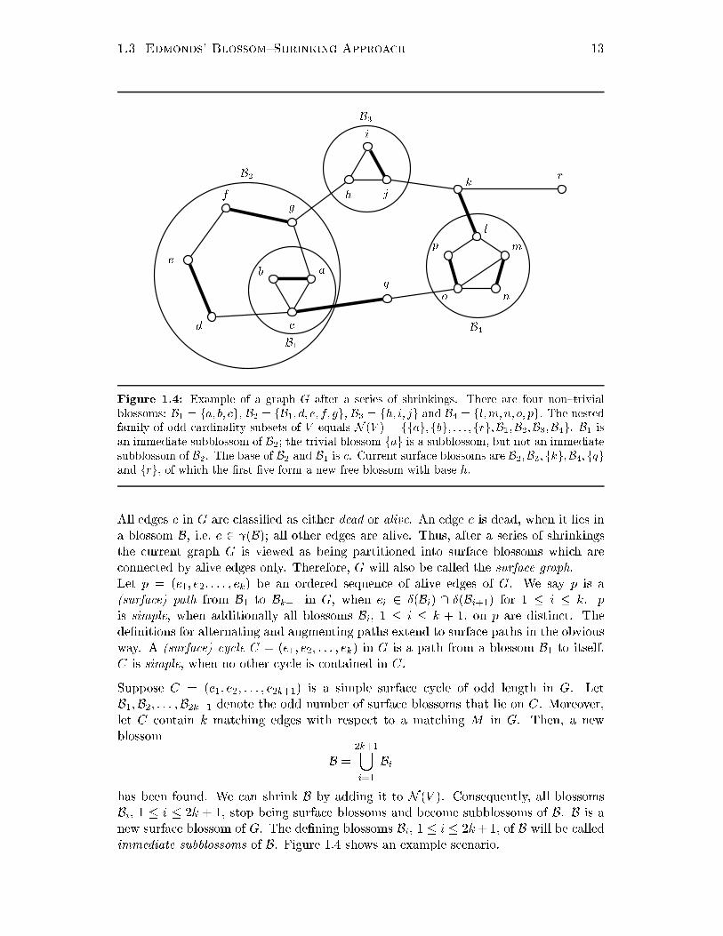
Figure 1.4: Example of a graph G after a series of shrinkings. There are four non{trivialblossoms: B1 = fa; b; g, B2 = fB1; d; e; f; gg, B3 = fh; i; jg and B4 = fl;m; n; o; pg. The nestedfamily of odd ardinality subsets of V equals N (V ) = ffag; fbg; : : : ; frg;B1;B2;B3;B4g. B1 isan immediate subblossom of B2; the trivial blossom fag is a subblossom, but not an immediatesubblossom of B2. The base of B2 and B1 is . Current surfa e blossoms are B2;B3; fkg;B4; fqgand frg, of whi h the �rst �ve form a new free blossom with base h.All edges e in G are lassi�ed as either dead or alive. An edge e is dead, when it lies ina blossom B, i.e. e 2 (B); all other edges are alive. Thus, after a series of shrinkingsthe urrent graph G is viewed as being partitioned into surfa e blossoms whi h are onne ted by alive edges only. Therefore, G will also be alled the surfa e graph.Let p = (e1; e2; : : : ; ek) be an ordered sequen e of alive edges of G. We say p is a(surfa e) path from B1 to Bk+1 in G, when ei 2 Æ(Bi) \ Æ(Bi+1) for 1 � i � k. pis simple, when additionally all blossoms Bi, 1 � i � k + 1, on p are distin t. Thede�nitions for alternating and augmenting paths extend to surfa e paths in the obviousway. A (surfa e) y le C = (e1; e2; : : : ; ek) in G is a path from a blossom B1 to itself.C is simple, when no other y le is ontained in C.Suppose C = (e1; e2; : : : ; e2k+1) is a simple surfa e y le of odd length in G. LetB1;B2; : : : ;B2k+1 denote the odd number of surfa e blossoms that lie on C. Moreover,let C ontain k mat hing edges with respe t to a mat hing M in G. Then, a newblossom B = 2k+1[i=1 Bihas been found. We an shrink B by adding it to N (V ). Consequently, all blossomsBi, 1 � i � 2k + 1, stop being surfa e blossoms and be ome subblossoms of B. B is anew surfa e blossom of G. The de�ning blossoms Bi, 1 � i � 2k+1, of B will be alledimmediate subblossoms of B. Figure 1.4 shows an example s enario.

14 Chapter 1. Mat hing TheoryAlgorithm 1.3.1 Generi algorithm to sear h for an augmenting path p from a freevertex r. Let G be the underlying graph and M a mat hing in G su h that r is free.let r be the only even vertex of Twhile there does not exist an alive edge e = uv with u+ 62 T and v+ 2 T fif an alive edge uv with u+ 2 T and v? 62 T exists flet b be the base of Bv and w denote the mate of b, with w 2 Bwmake Bv an odd and Bw an even labeled blossom of Tadd the edges uv and bw to Tgelse if an alive edge uv with u+ 2 T and v+ 2 T exists fdetermine the lowest ommon an estor Bl a of Bu and Bv in Tlet p1 = (e1; : : : ; e2j) be the alternating path from Bl a to Bu in T , andlet p2 = (e2j+2; : : : ; e2k+1) be the alternating path from Bv to Bl a in Tall surfa e blossoms on C = (p1; e2j+1 = uv; p2) de�ne a new blossom Bshrink B by making all surfa e blossoms on C to subblossoms of BB gets labeled even and all edges in (B) are onsidered to be deadgelse terminate, T is abandoned sin e no augmenting path for r existsgthere must exist an even length alternating surfa e path p00 from Bv to Br in Tp0 = (e; p00) is an augmenting surfa e path from Bu to Brraise p0 to an augmenting path p in the original graph G using Lemma 1.3.1By now we are well prepared to revise our sear h for an augmenting path. At the endwe give a generi algorithm that seeks an augmenting path in a general graph G. Thealgorithm is based on the nested view of G developed above and will be fundamentalfor the weighted mat hing problem.Let M be a mat hing in G and r a free vertex with respe t to M . As in the bipartite ase, an alternating tree T is grown from r. However, T forms a tree with respe t tothe surfa e blossoms of G only, and the edges used by the sear h are restri ted to beingalive. For the sake of on iseness, we denote the surfa e blossom to a vertex u of G byBu. Moreover, we stipulate that ea h vertex u retains the label of its surfa e blossomBu, and u is said to be in T , when Bu is ontained in T .Shortly, it will be ome apparent that non{trivial blossoms an o ur only as even treeblossoms in the unweighted mat hing ase. However, in the weighted mat hing aselater on, non{trivial blossoms will also o ur outside of T and an be even or odd treeblossoms. Therefore, we do some preparatory work by assuming non{trivial blossomsto be of any kind.Initially, T onsists of the even labeled vertex r+ only. The sear h assumes the followinglabeling for all surfa e blossoms outside of T : ea h free surfa e blossom is labeled evenand ea h mat hed surfa e blossom is unlabeled. Four ases have to be distinguished.Let uv be an alive edge with u+ 2 T and v? 62 T . The base b of Bv must be mat hed,sin e Bv is unlabeled. Let w denote the mate of b in Bw. T is extended by making Bv

1.3 Edmonds' Blossom{Shrinking Approa h 15Algorithm 1.3.2 Generi algorithm to ompute a maximum{ ardinality mat hing ina general graph G.let M be an arbitrary mat hing in Glabel all free verti es even and unlabel all mat hed verti esfor ea h vertex r in G fif r is mat hed ontinue with another vertexgrow an alternating tree T rooted in r as des ribed in Algorithm 1.3.1if an augmenting path p with respe t to M in G has been found frepla e M by the augmented mat hing M � punlabel all verti es ontained in Tdelete all non{trivial surfa e blossoms of Tdestroy Tgelse T has been abandoned ontinue with another vertexgM is a maximum{ ardinality mat hingan odd and Bw an even labeled tree blossom and taking uv and bw to T . This is whatwe will all a grow step hen eforth.Let us assume there exists an alive edge uv with u+ 2 T and v+ 2 T . We determinethe lowest ommon an estor surfa e blossom Bl a of Bu and Bv. That is, Bl a is the�rst blossom that is both on the surfa e tree path from Bu to Br and on the surfa etree path from Bv to Br. Noti e that from the way we built T , Bl a must be labeledeven. Let p1 = (e1; : : : ; e2j) denote the even length surfa e path from Bl a to Bu andp2 = (e2j+2; : : : ; e2k+1) the even length surfa e path from Bv to Bl a in T . Obviously,C = (p1; e2j+1 = uv; p2) is an odd length surfa e y le and moreover, a maximumnumber k of edges on that y le are mat hed, i.e. we have dete ted a blossom B. B isde�ned as the union of all surfa e blossoms Bi on C, with 1 � i � 2k + 1. Sin e forevery vertex v of B an even length alternating path to the base of B (this will a tuallybe the base of Bl a) exists, and therefore also an even length alternating path fromv to the root r of T , B gets labeled even.3 All blossoms Bi, 1 � i � 2k + 1, be omesubblossoms of B and ea h edge in (B) is no longer used by the sear h. That ompletesthe des ription of a so{ alled shrink step.When an alive edge uv with u+ 2 T and v+ 62 T is en ountered, an augmenting surfa epath p0 = (vu; p00) from Bv to Br is dire tly available. Here, p00 denotes the even lengthalternating surfa e path from Bu to Br in T . p0 an be lifted to an augmenting path pin the original graph G by repeatedly applying Lemma 1.3.1.Last, when none of the above ases applies T is abandoned, sin e no augmenting pathstarting in r exists. T retains its identity, i.e. all surfa e blossoms in T stay in T andretain their label. T will never be looked at again.When an alternating tree T is abandoned, there are no edges from any vertex u+ 2 T3A tually, that is the justi� ation for the label of a vertex being determined by its surfa e blossom.

16 Chapter 1. Mat hing Theoryto any other vertex vf?j+g 62 T . Moreover, ea h edge uv onne ting two even verti esu+ 2 T and v+ 2 T is dead, i.e. lies in a surfa e blossom B+ 2 T . Ea h odd surfa eblossom B�i 2 T (whi h is trivial in the unweighted mat hing ase) is mat hed by analive edge ij 2M with an even surfa e blossom B+j 2 T , and B+r 2 T is the only surfa eblossom that is free in T .The omplete sear h for an augmenting path in a general graph G is summarized inAlgorithm 1.3.1.Combining the idea of Algorithm 1.2.1 with the sear h just des ribed yields a generi algorithm for omputing a maximum{ ardinality mat hing in a general graph G asgiven in Algorithm 1.3.2.p qIn the rest of this se tion, we will prove optimality of M�, the mat hing obtained by Algo-rithm 1.3.2, and thus establish orre tness. The results to ome are interesting from a theo-reti al point of view. However, the optimality riteria for the weighted mat hing ase will beof another kind and only Algorithm 1.3.1 will be used. Therefore, the reader may also skipdire tly to the next se tion.Di�erent optimality riteria have evolved over several de ades. Two of them will be onsideredmore losely. The �rst is due to Edmonds [Edm65b℄ and is based on the notion of an odd set over. The se ond is known as the Tutte{Berge Formula.Assume M� leaves t verti es unmat hed. The ardinality of M is thus b(n � t)=2 , where ndenotes the number of verti es in G. For ea h free vertex ri, 1 � i � t, an alternating tree Ti,whi h has been abandoned by the sear h, is rooted in Bri . As we outlined above, ea h vertexu� 2 Ti, 1 � i � t, is mat hed with a surfa e blossom B+ 2 Ti and only the root blossom Briis free. Remember that all edges uv onne ting two even verti es must lie in the same blossomB+ 2 Ti for some 1 � i � t. All unlabeled verti es u? are mat hed with a vertex v? and forea h tree Ti, there exists no edge uv with u? and v+ 2 Ti.Let C(V ) be a family of pairwise disjoint odd ardinality subsets of V . C(V ) is alled an oddset over of G when for every edge e 2 E: e 2 Æ(v) for a singleton set fvg 2 C(V ), or otherwisee 2 (S) for a non{singleton set S 2 C(V ).The apa ity ap(S) of a set S 2 C(V ) is de�ned as ap(S) = (1 when S is a singleton set,bjSj=2 otherwise.As an easily be veri�ed, the total apa ity ap(C(V )) = PS2C(V ) ap(S) of an odd set overgives an upper bound for the ardinality of any mat hing in G, i.e. jM j � ap(C(V )).4Edmonds onstru ted an odd set over C(V ) of G having apa ity equal to the ardinality ofM� and thus proved M� to be maximum.C(V ) = fv� 2 Ti : 1 � i � kg [ fB+ 2 Ti : 1 � i � k, and B is non{trivialg:When U 6= ;, we hoose some u 2 U and add fug to C(V ). Additionally, U n u is added toC(V ), when jU j > 2.54Let M be a mat hing in G. Ea h edge e 2 M must be overed by some set S 2 C(V ) and thenumber of mat hing edges overed by some S 2 C(V ) is learly bounded above by ap(S).5Let us see why C(V ) does indeed form an odd set over. Ea h odd vertex v� 2 Ti, 1 � i � t,

1.3 Edmonds' Blossom{Shrinking Approa h 17Ea h odd vertex v overs exa tly 1 = ap(v) mat hing edge of M�. We argued above thatthe number of mat hed edges in an even surfa e blossom B equals bjBj=2 = ap(B). Finally,u overs exa tly 1 = ap(u) mat hing edge. If jU j > 2, all other b(jU j � 1)=2 = ap(U n u)mat hing edges are overed by U n u. Thus, we have jM�j = ap(C(V )) as desired. We an nowstate the optimality riteria whi h is due to Edmonds [Edm65b℄.Lemma 1.3.2 Let G = (V;E) be a graph and M a mat hing in G. Moreover, let C(V ) be anodd set over of G having apa ity ap(C(V )). Then, M is a maximum{ ardinality mat hingand C(V ) is an odd set over having minimum apa ity, i� jM j = ap(C(V )).Another interesting possibility to obtain an upper bound on the ardinality of a mat hing Min G is as follows.Let A � V be an arbitrary subset of verti es of G. Removing ea h vertex u 2 A and all itsin ident edges from G, results in a new graph denoted by G n A. Let C1; C2; : : : ; Ck be the onne ted omponents in G n A having an odd number of verti es. Ea h Ci ontains eithera free vertex, or there exists a mat hing edge uv 2 M with u 2 Ci and v 2 A. Sin e M isa mat hing, the endpoints in A of those edges must be distin t. Therefore, at most jAj su hmat hing edges exist. Consequently, we an on lude that at least k�jAj verti es must be freewith respe t to M . To put it di�erently, no more than n � (k � jAj) verti es an be mat hedby M .Let o (G) denote the number of onne ted omponents in G having an odd number of verti es.The ardinality of a mat hing M is thus bounded by jM j � b(n� o (G nA) + jAj)=2 , for anyA � V .Again, we show optimality of M�. Choose A = fv� 2 Ti : 1 � i � kg. Obviously, o (G n A)must be jAj + t, sin e that is the total number of even surfa e blossoms in all abandonedtrees Ti, 1 � i � k. Thus, the bound stated above be omes tight, i.e. jM�j = b(n � t)=2 =b(n � o (G n A) + jAj)=2 , and M� is maximum. The following optimality riterion for amaximum{ ardinality mat hing has just been proved. It is due to Berge [Ber58℄.Lemma 1.3.3 Let G = (V;E) be a graph having n verti es and M a mat hing in G. M is amaximum{ ardinality mat hing, i� a set A � V exists with jM j = b(n� o (G nA) + jAj)=2 .The dis ussion above and Lemma 1.3.3 immediately imply the following orollary whi h statesa ondition for the existen e of a perfe t mat hing. It was originally proved by Tutte [Tut47℄.Corollary 1.3.1 A graph G = (V;E) has a perfe t mat hing i� for every set A � V of verti eso (G nA) � jAj.As an aside, observe that Algorithm 1.3.2 will �nd a perfe t mat hing, if there exists any. Butit an even prove the non{existen e of a perfe t mat hing using Corrollary 1.3.1. To see this, onsider any abandoned tree Ti. Let A denote the set of odd verti es in Ti. Sin e the number ofeven labeled surfa e blossoms in Ti equals jAj+1, it is o (G nA) = jAj+1 > jAj and we havethus proved that no perfe t mat hing exists. In on lusion, we an state that Algorithm 1.3.2 an solve maximum{ ardinality perfe t mat hing problems as well.x y overs all its in ident edges. All edges lying in an even labeled surfa e blossom B+ 2 Ti are overed byB 2 C(V ). Edges onne ting two verti es of U are overed by u or lie in (U n u) and are hen e overedby U n u. Finally, no other edges exist as stated before.

18 Chapter 1. Mat hing Theory1.4 LP Formulations for Weighted Mat hing ProblemsIn the pre eding se tions, important mat hing on epts su h as augmenting paths havebeen introdu ed. Further, we a quired a generi algorithm that an solve both variantsof the maximum{ ardinality mat hing problem. The stated results serve as a goodbasis for the weighted ase onsidered in this and the subsequent se tions.Fundamental �ndings in the area of ombinatorial optimization will guide us to a generi algorithm for the weighted mat hing problem. We assume familiarity with terms su has linear programming formulations, relaxation, duality theory (weak and strong du-ality, omplementary sla kness) as well as the on epts behind primal{dual methods.For extensive sour es on erning these subje ts, see Bertsimas and Tsitsiklis [BT97℄,Papadimitriou and Steiglitz [PS82℄ and Chv�atal [Chv83℄.We start with the dis ussion of linear programming formulations for the weightedmat hing problem.1.4.1 LP Formulation for the Weighted Mat hing ProblemLet G = (V;E;w) be an instan e of the maximum{weight mat hing problem. Themaximum{weight mat hing problem an be formulated as a zero{one integer linearprogramming problem. An in iden e ve tor x is asso iated with the edges of G. Ea h omponent xe is a de ision variable having value 0 or 1. The relation between thein iden e ve tor x and a mat hing M is as follows:xe = (0 if e does not belong to the mat hing M ,1 if e does belong to the mat hing M .An in iden e ve tor x orresponding to a given mat hing M is alled the hara teristi ve tor of M .Let S � E be a subset of edges and x an in iden e ve tor asso iated with the edges E ofG. x(S) is de�ned as the sum over all omponents xe with e 2 S, i.e. x(S) =Pe2S xe.We are now able to formulate the maximum{weight mat hing problem as a zero{oneinteger linear program (iwm):(iwm) maximize wTxsubje t to x(Æ(u)) � 1 for all u 2 V , (1)xe 2 f0; 1g for all e 2 E. (2)(iwm)(1) assures that ea h vertex has at most one in ident edge that is mat hed. Notethat ea h optimal solution x of (iwm) orresponds to a maximum{weight mat hing M .And onversely, every hara teristi ve tor x to a maximum{weight mat hing M is anoptimal solution to (iwm). Therefore, (iwm) does in fa t formulate the maximum{weight mat hing problem.A standard te hnique in ombinatorial optimization is to relax the zero{one onstraint(iwm)(2) whi h yields the linear programing relaxation (wm').

1.4 LP Formulations for Weighted Mat hing Problems 19(wm') maximize wTxsubje t to x(Æ(u)) � 1 for all u 2 V , (1)xe � 0 for all e 2 E. (2)Unfortunately, (wm') does not have zero{one solutions only.6 To see this, onsider agraph G = (V;E) having three verti es V = fa; b; g that lie on a odd length y le,i.e. E = fab; b ; ag. Assume further that we = 1 for all edges e 2 E. Then, xe = 1=2 forea h edge e of G is an optimal solution to (wm') having obje tive value 3=2. However,x is not a solution to (iwm) (the obje tive value of an optimal solution to (iwm) is 1).Consequently, the two formulations (iwm) and (wm') are not equal, or to put it dif-ferently, (wm') is said to be not as strong as (iwm). A measure for the strength ofa linear programming relaxation is the loseness of its feasible set to the onvex hullde�ned by the feasible in iden e ve tors of the original integer program.In general, the feasible set F (lp) to a linear programming formulation (lp) onsists ofall feasible in iden e ve tors to (lp). For example,F (wm') = fx : x satis�es (wm')(1) and (wm')(2)g:The onvex hull P(lp) of a feasible set F (lp) an be seen as a polyhedron spanned byF (lp).7For an integer linear programming formulation (ilp) and its relaxation (lp') the re-lation P(ilp) � P(lp') always holds, whereas one annot expe t that the opposite doestoo. The relation between P(iwm) and P(wm') is a perfe t example.Theorem 1.4.1 Two linear programming formulations (lp) and (lp') are equallystrong, i� P(lp) = P(lp').The question is, whether there exists a linear programming formulation similar to (wm')that is moreover as strong as (iwm).Let O denote the set of all non{singleton odd ardinality subsets of V :O = fB � V : jBj is odd and jBj � 3g:Consider the linear programming formulation (wm) below.6However, the two linear programing formulations (wm') and (iwm) have been proved to be equiv-alent for the bipartite weighted mat hing problem. The proof is due to Birkho� [Bir46℄.7The onvex hull P of a �nite set S = fx1; x2; : : : ; xkg 2 Rn is de�ned as the set of all onvex ombinations of S:P = fx =Pki=1 �ixi : Pki=1 �i = 1, xi 2 S and �i � 0, 1 � i � kg:More pre isely, we would have to distinguish between a polyhedron P(lp) whi h is de�ned by (i.e. isequal to) its feasible set F (lp) and a polyhedron P(lp) whi h is de�ned by the onvex hull of its feasibleset F (lp) (e.g. in ases where (lp) is an integer linear program). However, we do not wish to go into thedetails of polyhedral ombinatori s at this point. Instead, for a more extensive dis ussion on erningthese aspe ts, the interested reader is referred to Cook et al. [CCPS98℄ and Bertsimas and Tsitsiklis[BT97℄.

20 Chapter 1. Mat hing Theory(wm) maximize wTxsubje t to x(Æ(u)) � 1 for all u 2 V , (1)x( (B)) � bjBj=2 for all B 2 O, (2)xe � 0 for all e 2 E. (3)(wm) equals (wm') ex ept that a new series of onstraints (wm)(2) has been added.(wm)(2) states, that the number of mat hed edges in (B), where B � V is a non{singleton odd ardinality set, is bounded above by bjBj=2 . Note that (wm)(2) oin ideswith one's intuition. It an easily be observed that ea h hara teristi ve tor x to agiven mat hing M must satisfy (wm)(1){(3) and therefore: P(iwm) � P(wm).What onsequen es does the additional onstraint (wm)(2) entail? As before, let usregard the graph G onsisting of an odd y le only. Setting xe = 1=2 for all edges of Gis not a feasible solution to (wm), sin e x( (fa; b; g)) = 3=2 � 1.The idea arises that (wm) is a stronger formulation than (wm'). And indeed, as thefollowing lemma shows, the linear programming formulation (wm) is not only strongerthan (wm'), but as strong as (iwm).Lemma 1.4.1 Let P(iwm) and P(wm) represent the polyhedron of (iwm) and (wm),respe tively. Then P(iwm) = P(wm).Lemma 1.4.1 is one of the ornerstones of the weighted mat hing theory. It is due toEdmonds. Generally, one an prove Lemma 1.4.1 either dire tly, or by an algorithmi proof.We will do so by the latter method, i.e. we develop an algorithm that omputes amat hingM and moreover, the hara teristi ve tor x to M will be an optimal solutionto (wm). Further details are deferred to Se tion 1.6. Similar algorithmi proofs an befound in Pulleyblank [Pul95℄ and Cook et al. [CCPS98℄.The dire t proof is omplex and not given here. Details an be found in the originalwork of Edmonds [Edm65a℄. Cook et al. [CCPS98, Chapter 6℄ and Lov�asz and Plummer[LP86℄ are also ex ellent sour es.1.4.2 LP Formulation for the Weighted Perfe t Mat hing ProblemThe linear programming formulation for the maximum{weight perfe t mat hing prob-lem slightly di�ers from (wm) and will be sket hed next. In Se tion 1.5 we will seethat under ertain onditions, ea h maximum{weight perfe t mat hing problem an beredu ed to the maximum{weight mat hing problem and ontrariwise. Taking that fa tinto onsideration, one may wonder if it is worth the e�ort to inspe t the weightedperfe t mat hing ase separately. However, the di�eren es between those two problemsregarding linear programming formulation aspe ts are interesting to see and, more-over, both problems an be in orporated into one generi algorithm easily as, will beexploited in Se tion 1.6.Again, we start with the integer linear program. Sin e every vertex has to be mat hed

1.4 LP Formulations for Weighted Mat hing Problems 21in the maximum{weight perfe t mat hing problem, the primal ondition (iwm)(1)be omes an equality onstraint:(iwpm) maximize wTxsubje t to x(Æ(u)) = 1 for all u 2 V , (1)xe 2 f0; 1g for all e 2 E. (2)In the perfe t ase, too, the linear programming relaxation of (iwpm) is not as strongas (iwpm) itself. But as in the non{perfe t ase, adding a new series of onstraintshelps. The orresponding linear program is (wpm).(wpm) maximize wTxsubje t to x(Æ(u)) = 1 for all u 2 V , (1)x( (B)) � bjBj=2 for all B 2 O, (2)xe � 0 for all e 2 E. (3)At this point one observes that the formulation of (wm) is a generalization of (wpm),sin e P(wpm) is a fa e of P(wm). The following lemma states that (iwpm) is as strongas (wpm).Lemma 1.4.2 Let P(iwpm) and P(wpm) represent the polyhedron of (iwpm) and(wpm), respe tively. Then P(iwpm) = P(wpm).As for Lemma 1.4.1, the generi algorithm in Se tion 1.6 will prove orre tness of thestated lemma. For alternative proofs all referen es given for Lemma 1.4.1 apply.1.4.3 An Alternative LP Formulation for the Weighted Perfe tMat hing ProblemIn Se tion 1.6 we will develop a primal{dual method that omputes an optimal solutionto the linear programming formulations given above. The details of that method dependon those �xed formulations. However, an alternative linear programming formulationfor the maximum{weight perfe t mat hing problem exists and will be the subje t ofthis se tion. The pros and ons of that alternative formulation with respe t to theresulting primal{dual method will be dis ussed in detail in Se tion 1.6.5.In both ases, i.e. the perfe t and non{perfe t weighted mat hing problem, we added aseries of onstraints to the relaxation of the integer linear program in order to obtain alinear program that is as strong as its integer linear program. Those onstraints havebeen of the form: x( (B)) � bjBj=2 for all B 2 O: (1.1)However, for the weighted perfe t mat hing problem, the same e�e t an be a hievedby a di�erent type of onstraint:x(Æ(B)) � 1 for all B 2 O: (1.2)

22 Chapter 1. Mat hing Theory(1.2) means that at least one edge that leaves a non{singleton odd ardinality set B,i.e. is part of Æ(B), must be mat hed.The alternative formulation for the maximum{weight perfe t mat hing problem is givenin (wpm*).(wpm*) maximize wTxsubje t to x(Æ(u)) = 1 for all u 2 V , (1)x(Æ(B)) � 1 for all B 2 O, (2)xe � 0 for all e 2 E. (3)As mentioned above, it an be shown that (wpm*) is as strong as (iwpm). Thus,(wpm*) is indeed an alternative to (wpm).1.5 Redu tionsWe intend to use this se tion to show that ea h instan e of the maximum{weightmat hing problem an be redu ed to an instan e of the maximum{weight perfe t mat- hing problem. Moreover, assuming the availability of a te hnique to dis over thenon{existen e of a perfe t mat hing, the ontrary an be a hieved as well.We will des ribe these redu tions by means of a transformation � su h that(i1) for ea h instan e G = (V;E;w) of the maximum{weight mat hing problem, amaximum{weight perfe t mat hing M 0 in G0 = �(G) an be translated to amaximum{weight mat hing M in G, and(i2) under the assumption that a perfe t mat hing exists for an arbitrary in-stan e G0 = (V 0; E0; w0) of the maximum{weight perfe t mat hing problem,a maximum{weight mat hing M in G = ��1(G0) orresponds to a maximum{weight perfe t mat hing M 0 in G0.First, � will be onstru ted suiting (i1) and after that the inverse transformation ��1satisfying (i2) will be given.1.5.1 Redu ing theWeighted Mat hing Problem to the Weighted Per-fe t Mat hing ProblemLet G = (V;E;w) be an instan e of the maximum{weight mat hing problem. We givea transformation �(G) = G0, where G0 = (V 0; E0; w0), and then pro eed to show thatG0 satis�es (i1).Assume, eG = (eV ; eE; ew) is a opy of G. For ea h vertex u, edge e and weight we of G,we denote the orresponding vertex, edge and weight in eG by eu, ee and ewee, respe tively.Consider the graph G0 that onsists of G and eG. Moreover, let G0 have additional zero{ ost edges from ea h vertex u of G to eu of eG. More pre isely, G0 is given as V 0 = V _[ eV

1.5 Redu tions 23and E0 = E _[ eE [ fueu : u 2 V and eu 2 eV g:The weight fun tion w0 of G0 is de�ned as:w0e0 = 8><>:we0 when e0 2 E,ewe0 when e0 2 eE,0 when e0 = ueu with u 2 V and eu 2 eV .Lemma 1.5.1 Let G0 = �(G) as given above. Ea h maximum{weight perfe t mat- hing M 0 in G0 then orresponds to a maximum{weight mat hing M in G.Proof:Let M 0 be a maximum{weight perfe t mat hing in G0. The di�eren eM 0 n fueu : u 2 V and eu 2 eV g =M _[ fMde omposes into M � E and fM � eE. Sin e M 0 is of maximum weight, M must be amaximum{weight mat hing in G.Conversely, let M be a maximum{weight mat hing in G and fM the orrespondingmat hing in eG. ThenM 0 =M [ fM [ fueu 2 E0 : u free in G and eu free in eGgis a perfe t mat hing in G0 with weight w0(M 0) = 2w(M). �The stated lemma is often used to redu e the proof of Lemma 1.4.1 to the proof ofLemma 1.4.2.1.5.2 Redu ing the Weighted Perfe t Mat hing Problem to theWeighted Mat hing ProblemConsider an instan e G0 = (V 0; E0; w0) of the maximum{weight perfe t mat hing prob-lem. We will onstru t a transformation ��1 that gives us an instan e ��1(G0) = G,with G = (V;E;w), of the maximum{weight mat hing problem satisfying (i2). How-ever, we wish to emphasize that the redu tion to be stated is orre t only when a perfe tmat hing does indeed exist in G0.In the dis ussion that follows, we assume that all edge weights of G0 are non{negative.We may make this assumption, sin e the weighted perfe t mat hing problem is nota�e ted when all edge weights are modi�ed by adding a onstant = maxfjwej : e 2 Eg.De�ne G = (V;E;w) with V = V 0 and E = E0. The edge weights in G will be setsu h that ea h maximum{weight mat hing M in G is perfe t. This an be a hieved byadding a positive value L to the original edge weights of G0: we = w0e + L.Choosing L su h that the total weight w(fM ) of ea h perfe t mat hing fM in G is largerthan the total weight of any non{perfe t mat hingM in G yields the desired result. Letn = jV j denote the number of verti es of G; n is assumed to be even, sin e otherwise no

24 Chapter 1. Mat hing Theoryperfe t mat hing exists in G0. Moreover, let C = max fw0e : e 2 E0g be the maximumedge weight in G0. By the de�nition of w, we have C + L � we � L. The totalweight w(fM ) of ea h perfe t mat hing fM is thus bounded below by jfM j L = (n=2) L.Conversely, the total weight w(M) of a non{perfe t mat hing M annot be more thanjM j (C + L). Hen e, hoosing L su h that the relation(n=2) L > jM j (C + L) (1.3)holds, assures that ea h maximum{weight mat hingM in G will be perfe t. The right{hand side of (1.3) maximizes for jM j = (n=2) � 1, sin e that is the largest ardinalityof a non{perfe t mat hing possible. Therefore, hoosing L := (n=2) C > ((n=2)� 1) Chas the desired e�e t.Lemma 1.5.2 LetG = ��1(G0) as given above and assume a perfe t mat hing exists inG0. Ea h maximum{weight mat hing M in G then orresponds to a maximum{weightperfe t mat hing M 0 in G0.Proof:Let M be a maximum{weight mat hing in G. From the onstru tion above, it immedi-ately follows that M must be perfe t. The total weight of a maximum{weight perfe tmat hing in G0 is thus w0(M) = w(M)� jM j L = w(M)� (n=2) L.Conversely, let M 0 be a maximum{weight perfe t mat hing in G0 having total weightw0(M 0). M 0 is then a perfe t mat hing in G of weight w(M 0) = w0(M 0) + jM j L =w0(M 0) + (n=2) L. Due to the onstru tion of G, no non{perfe t mat hing an havetotal weight larger than or equal to w(M 0). Thus, M 0 is a maximum{weight mat hingin G. �Ea h maximum{weight perfe t mat hing problem an thus be solved by an algorithmfor the maximum{weight mat hing problem using Lemma 1.5.2 and a further te hniqueto dis over the non{existen e of a perfe t mat hing in G (for example Corrollary 1.3.1).Mehlhorn and N�aher [MN99℄ use a similar onstru tion to for e a maximum{weightbipartite mat hing algorithm to �nd a maximum{weight mat hing along all maximum{ ardinality bipartite mat hings.1.6 Primal{Dual MethodIn Se tion 1.4.1 a linear programing formulation for the maximum{weight mat hingproblem was introdu ed. Based on that formulation, we will use duality theory toobtain a �rst high{level primal{dual method to ompute a maximum{weight mat hingto a given instan e. A primal{dual method based on the maximum{weight perfe tmat hing problem formulation of Se tion 1.4.2 will then be outlined.Edmonds' blossom{shrinking approa h will be extended in Se tion 1.6.3 su h that itbe omes a on rete derivation of those primal{dual methods. The resulting generi algorithm establishes orre tness of Lemma 1.4.1 and Lemma 1.4.2 and will serve asthe fundamental approa h for our implementations.

1.6 Primal{Dual Method 25We will omplete this se tion by showing a useful property of the dual solution tothe maximum{weight mat hing and maximum{weight perfe t mat hing problem and,moreover, dis uss the pros and ons of a similar algorithm for the maximum{weightperfe t mat hing problem using the alternative formulation of Se tion 1.4.3.1.6.1 Primal{Dual Method for the Maximum{Weight Mat hingProblemWe repeat the linear programing formulation of the maximum{weight mat hing problem onsidered in Se tion 1.4.1:(wm) maximize wTxsubje t to x(Æ(u)) � 1 for all u 2 V , (1)x( (B)) � bjBj=2 for all B 2 O, (2)xe � 0 for all e 2 E. (3)We will use duality theory in order to derive a primal{dual method that omputesan optimal solution to (wm). The main idea is to ompute a mat hing M whose hara teristi ve tor x is a feasible and moreover optimal solution to (wm). We willassure optimality of x by a feasible solution to the dual linear program of (wm) thatsatis�es all omplementary sla kness onditions with x.The dual linear program (wm) to (wm) is given next. Ea h vertex u and ea h non{singleton odd ardinality set B has an asso iated dual variable yu and zB, respe tively.(wm) minimize Xu2V yu + XB2O bjBj=2 zBsubje t to yu � 0 for all u 2 V , (1)zB � 0 for all B 2 O, (2)yu + yv + XB2Ouv2 (B) zB � wuv for all uv 2 E. (3)We will all yu and zB the dual value, or alternatively the potential of vertex u andblossom B. (wm)(3) states that the potentials of the endpoints of an edge e = uv plusthe sum of all potentials of non{trivial odd ardinality sets ontaining that edge mustbe greater or equal to the weight of e.To simplify further notations, we introdu e the notion of the redu ed ost of an edge e.De�nition 1.6.1 (Redu ed Cost) Let (y; z) be a solution to the dual linear program(wm). The redu ed ost �uv of an edge e = uv with respe t to (y; z) is de�ned as:�uv = yu + yv � wuv + XB2Ouv2 (B) zB:An edge e = uv is alled tight, when its redu ed ost �uv equals zero. Note that(wm)(3) an be repla ed by �uv � 0 for all edges uv of E. Thus, (wm)(3) assures thatthe redu ed ost of ea h edge is non{negative.

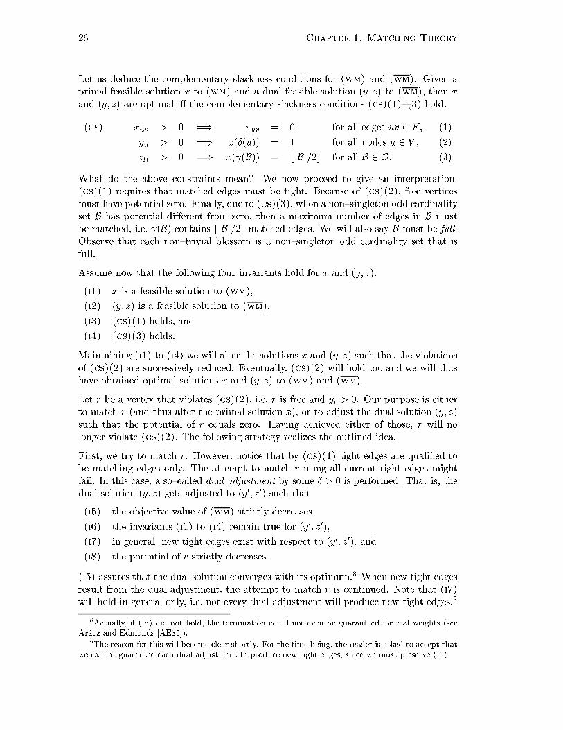
26 Chapter 1. Mat hing TheoryLet us dedu e the omplementary sla kness onditions for (wm) and (wm). Given aprimal feasible solution x to (wm) and a dual feasible solution (y; z) to (wm), then xand (y; z) are optimal i� the omplementary sla kness onditions ( s)(1){(3) hold.( s) xuv > 0 =) �uv = 0 for all edges uv 2 E, (1)yu > 0 =) x(Æ(u)) = 1 for all nodes u 2 V , (2)zB > 0 =) x( (B)) = bjBj=2 for all B 2 O. (3)What do the above onstraints mean? We now pro eed to give an interpretation.( s)(1) requires that mat hed edges must be tight. Be ause of ( s)(2), free verti esmust have potential zero. Finally, due to ( s)(3), when a non{singleton odd ardinalityset B has potential di�erent from zero, then a maximum number of edges in B mustbe mat hed, i.e. (B) ontains bjBj=2 mat hed edges. We will also say B must be full.Observe that ea h non{trivial blossom is a non{singleton odd ardinality set that isfull.Assume now that the following four invariants hold for x and (y; z):(i1) x is a feasible solution to (wm),(i2) (y; z) is a feasible solution to (wm),(i3) ( s)(1) holds, and(i4) ( s)(3) holds.Maintaining (i1) to (i4) we will alter the solutions x and (y; z) su h that the violationsof ( s)(2) are su essively redu ed. Eventually, ( s)(2) will hold too and we will thushave obtained optimal solutions x and (y; z) to (wm) and (wm).Let r be a vertex that violates ( s)(2), i.e. r is free and yr > 0. Our purpose is eitherto mat h r (and thus alter the primal solution x), or to adjust the dual solution (y; z)su h that the potential of r equals zero. Having a hieved either of those, r will nolonger violate ( s)(2). The following strategy realizes the outlined idea.First, we try to mat h r. However, noti e that by ( s)(1) tight edges are quali�ed tobe mat hing edges only. The attempt to mat h r using all urrent tight edges mightfail. In this ase, a so{ alled dual adjustment by some Æ > 0 is performed. That is, thedual solution (y; z) gets adjusted to (y0; z0) su h that(i5) the obje tive value of (wm) stri tly de reases,(i6) the invariants (i1) to (i4) remain true for (y0; z0),(i7) in general, new tight edges exist with respe t to (y0; z0), and(i8) the potential of r stri tly de reases.(i5) assures that the dual solution onverges with its optimum.8 When new tight edgesresult from the dual adjustment, the attempt to mat h r is ontinued. Note that (i7)will hold in general only, i.e. not every dual adjustment will produ e new tight edges.98A tually, if (i5) did not hold, the termination ould not even be guaranteed for real weights (seeAr�aoz and Edmonds [AE85℄).9The reason for this will be ome lear shortly. For the time being, the reader is asked to a ept thatwe annot guarantee ea h dual adjustment to produ e new tight edges, sin e we must preserve (i6).

1.6 Primal{Dual Method 27Eventually, after a series of dual adjustments either suÆ iently many tight edges willexist su h that r an be mat hed, or the potential of r will drop to zero (due to (i8)).We summarize the dis ussed primal{dual method in Algorithm 1.6.1.Algorithm 1.6.1 Generi primal{dual method for the maximum{weight mat hingproblem.let x and (y; z) satisfy (i1) to (i4)while there exists a free vertex r with yr > 0 frepeat ftry to mat h r using tight edges onlyif r is not mat hed yetperform dual adjustment by Æ > 0 su h that (i5) to (i8) holdg until yr = 0 or r is mat hedgThe only missing details that have to be �lled in are how to �nd the initial feasiblesolutions x and (y; z) that satisfy (i1) to (i4), how to mat h free verti es using tightedges and how to perform a dual adjustment satisfying (i5) to (i8). We will ome ba kto these details in Se tion 1.6.3.1.6.2 Di�eren es in Weighted Perfe t Mat hing CaseSome minor hanges in the primal{dual method ensue for the maximum{weight perfe tmat hing problem. (wpm) introdu ed in Se tion 1.4.2 is used as the linear programingformulation for the maximum{weight perfe t mat hing problem.(wpm) maximize wTxsubje t to x(Æ(u)) = 1 for all u 2 V , (1)x( (B)) � bjBj=2 for all B 2 O, (2)xe � 0 for all e 2 E. (3)(wpm) equals (wm) ex ept that (wpm)(1) is an equality onstraint. Consequently,the non{negativity onstraints for all verti es in (wm) do not o ur in the dual linearprogram (wpm) of (wpm).(wpm) minimize Xu2V yu + XB2O bjBj=2 zBsubje t to zB � 0 for all B 2 O, (1)yu + yv + XB2Ouv2 (B) zB � wuv for all uv 2 E. (2)Thus, the omplementary sla kness onditions for a primal solution x of (wpm) and adual solution (y; z) of (wpm) are omprised of ( s)(1) and ( s)(3) only. We repeatthem as (p s)(1) and (p s)(2) below:

28 Chapter 1. Mat hing Theory(p s) xuv > 0 =) �uv = 0 for all edges uv 2 E, (1)zB > 0 =) x( (B)) = bjBj=2 for all B 2 O. (2)The des ription and arguments given for the non{perfe t ase no longer make sensenow. In the perfe t ase, we therefore maintain primal and dual solutions x and (y; z)that satisfy the invariants (j1) to (j4).(j1) x satis�es all onditions of (wpm) ex ept (wpm)(1),(j2) (y; z) is a feasible solution to (wpm),(j3) (p s)(1) holds, and(j4) (p s)(2) holds.Gradually, the violations of (wpm)(1) are de reased su h that in the end, x be omes aprimal feasible solution and thus is optimal, or one dis overs that the obje tive value of(wpm) is unbounded and therefore, no perfe t mat hing exists (by weak duality). Asbefore, tight edges are used to mat h a free vertex r. If the urrent tight edges do notsuÆ e to mat h r, a dual adjustment by Æ > 0 is performed. Æ must be hosen su hthat(j5) the obje tive value of (wpm) stri tly de reases,(j6) the invariants (j1) to (j4) remain true for the adjusted dual solution (y0; z0),(j7) in general, new tight edges exist with respe t to (y0; z0).The obje tive value of (wpm) is unbounded, when Æ an be made arbitrarily large,i.e. Æ =1. The modi�ed generi algorithm redu es to:Algorithm 1.6.2 Generi primal{dual method for the maximum{weight perfe t mat- hing problem.let x and (y; z) satisfy (j1) to (j4)while there exists a free vertex r frepeat ftry to mat h r using tight edges onlyif r is not mat hed yet f hoose Æ > 0 su h that (j5) to (j7) holdif Æ =1 terminate, sin e no perfe t mat hing existselse perform dual adjustment by Ægg until r is mat hedg1.6.3 The Blossom{Shrinking Approa h RevisitedBased on the primal{dual methods dis ussed in the pre eding se tions we will extendEdmonds' blossom{shrinking approa h (see Se tion 1.3) su h that it an solve instan esof the weighted mat hing problem (non{perfe t and perfe t). We will �rst fo us on the

1.6 Primal{Dual Method 29maximum{weight mat hing problem and outline the di�eren es for the perfe t mat hing ase thereafter.The following three details are still open and will be �lled in next:1. onstru ting the initial solutions x and (y; z) to (wm) and (wm) that satisfy (i1)to (i4),2. mat hing a free vertex r with non{zero potential using tight edges only, and3. performing a dual adjustment by Æ > 0 and assuring the validity of (i5) to (i8).Throughout this se tion, let G = (V;E;w) be an instan e of the maximum{weightmat hing problem. x will denote the hara teristi ve tor to a mat hing M of G. Wewill often not distinguish between a mat hing M and its hara teristi ve tor x, anduse one notion for the other.Finding Initial SolutionsClearly, the empty mat hing M = ;, i.e. xe = 0 for ea h edge e 2 E, is a feasiblesolution to (wm). For ea h vertex u the potential is set to yu = max fwe=2 : e 2 Æ(u)g.The approa h will use the potentials zB of blossoms only. That is, the potential zB ofea h non{singleton odd ardinality set is regarded as being set to zB = 0. Ex eptionsare the potentials that are asso iated with a non{trivial blossom B; these an have valuezB > 0. Initially, no non{trivial blossoms exist. We thus obtain a feasible solution (y; z)to the dual linear program (wm).Moreover, note that x and (y; z) satisfy both onditions ( s)(1) and ( s)(3). Insummary, we an state that x and (y; z) meet the invariants (i1) to (i4).Di�erent possibilities to obtain better initial solutions will be the subje t of Se tion 3.5.For now, assume we start with the solutions x and (y; z) above.Redu ing the Violations of ( s)(2)Consider a free vertex r with non{zero potential yr > 0. First, we will des ribe theattempt to mat h r using tight edges only. The dual adjustment step, whi h is trig-gered when the sear h does not su eed due to insuÆ iently many tight edges, will be onsidered more losely afterwards.Mat hing a free vertex r using tight edges. From the dis ussion in Se tion 1.3one immediately observes that the task of mat hing r redu es to a sear h for an aug-menting path starting with r. Therefore, we grow an alternating tree T rooted at ras des ribed in Algorithm 1.3.1. However, in the weighted mat hing ase it is ru ialthat only tight edges are used by the sear h in order to preserve ( s)(1). All details ofAlgorithm 1.3.1 apply.In the ase where a blossom B is shrunk, B is full, and, therefore, its potential zBbe omes a essible for future dual adjustments, as will be explained below.

30 Chapter 1. Mat hing TheoryWhen an augmenting path p onsisting of tight edges has been found, the urrentmat hing M is augmented by p to M 0. As a result, r will be mat hed thereafter andthe new hara teristi ve tor x0 ofM 0 no longer violates ( s)(2), as desired. All surfa eblossoms in T get unlabeled and T is destroyed. However, note the following di�eren e.In the unweighted mat hing ase, all non{trivial surfa e blossoms have been deletedwhen T was destroyed (see also Algorithm 1.3.2). For the weighted mat hing ase thesituation is di�erent. It is ru ial that non{trivial surfa e blossoms with zB > 0 retaintheir identity; deleting them would hange the dual solution. As a onsequen e, non{trivial blossoms an o ur outside of an alternating tree or as even or odd labeled treeblossoms.When T is abandoned by the sear h this is due to the non{existen e of further tightedges uv in ident to any vertex u+ 2 T . In su h ases, a dual adjustment is initiated asdes ribed below. New tight edges might exist thereafter and the sear h resumes withT .Performing a dual adjustment. Consider a situation where the sear h for an aug-menting path from r fails be ause there are no more tight edges in ident to any vertexu+ 2 T .We want to alter the potentials (y; z) of the verti es and non{singleton odd ardinalitysets su h that (i5) to (i8) are met. One way to a hieve this is by adjusting (y; z) to(y0; z0) as stated below. The value of Æ > 0 will be determined shortly.y0v = yv � Æ for all v+ 2 T ;y0v = yv + Æ for all v� 2 T ;y0v = yv for all vf?j+g 62 T ;z0B = zB + 2Æ for all B+ 2 T ;z0B = zB � 2Æ for all B� 2 T ;z0B = zB for all Bf?j+g 62 T :Note that the adjustment has to be interpreted as follows. The potentials of all verti esin T are adjusted | in luding those that are ontained in a non{trivial blossom. Onthe other hand, a potential zB of a non{singleton odd ardinality set B is only adjustedwhen B is a non{trivial surfa e blossom of G.We demonstrate that all onditions stated above are met when a dual adjustment byan appropriate value Æ is performed.First, we laim that the obje tive value of (wm) stri tly de reases by Æ. Sin e Æ > 0,that will imply the orre tness of (i5). We onsider the rate of hange �f = f 0 � f inthe obje tive value of (wm), where f and f 0 denote the obje tive value before and afterthe dual adjustment, respe tively. The rate of hange that is ontributed to �f by atrivial blossom u or non{trivial blossom B is denoted by �fu and �fB. An odd labeledtrivial surfa e blossom v� 2 T obviously ontributes �fv� = Æ to �f . Analogously,�fv+ = �Æ for an even labeled trivial surfa e blossom v+ 2 T . Let B� be an odd

1.6 Primal{Dual Method 31labeled non{trivial surfa e blossom of T . Then,�fB� = jBjÆ + bjBj=2 (�2Æ) = jBjÆ � (jBj � 1)Æ = Æ:Analogously, for an even labeled non{trivial surfa e blossom B+ 2 T we have:�fB+ = jBj(�Æ) + bjBj=2 (2Æ) = �jBjÆ + (jBj � 1)Æ = �Æ:We an on lude the argument now by observing that T always ontains more eventhan odd surfa e blossoms (trivial or non{trivial). More pre isely, let n+ denote thenumber of even surfa e blossoms in T . Correspondingly, let n� be the total number ofodd surfa e blossoms in T . Sin e ea h even surfa e blossom ex ept the root is mat hedwith an odd surfa e blossom in T , we have: n+ = n� + 1. The total rate of hange inthe obje tive value is therefore �f = n+(�Æ) + n�Æ = �Æ.Let us prove that invariant (i6) holds. We start with the feasibility onditions (i1) and(i2). x stays feasible if it was so before the dual adjustment, sin e x is not altered atall.Ensuring that the adjusted dual solution (y0; z0) is dual feasible entails some restri tionson the value of Æ. First, Æ annot be larger than the smallest potential of an evenlabeled vertex u+ 2 T . Se ond, the potential of all non{trivial blossoms must staynon{negative, and therefore Æ is bounded above by the minimal value zB=2 of an oddnon{trivial surfa e blossom B� 2 T . Finally, the redu ed ost of all edges must benon{negative after the dual adjustment. This point demands loser inspe tion.We only onsider edges e = uv with at least one endpoint in T ; the redu ed osts ofedges having none of its endpoints in T do not hange. Let �uv denote the redu ed ostof e before the dual adjustment and assume further that e does not lie in a blossom B,i.e. e 62 (B) for a blossom B. We distinguish �ve ases.Case 1: u+ 2 TCase 1a: u+ 2 T and v+ 2 Tboth endpoints of e are de reased by Æ. Sin e the new redu ed ost �uv � 2Æ is restri ted to being non{negative, we obtain anupper bound of Æ � �uv=2.Case 1b: u+ 2 T and vf?j+g 62 Tthe redu ed ost �uv of e will hange by �Æ, resulting in anotherbound: Æ � �uvCase 2: u+ 2 T and v� 2 Tsin e u is de reased and v in reased by Æ, the redu ed ost �uv of e will not hange.Case 3: u� 2 TCase 3a: u� 2 T and v� 2 Tthe potential of ea h endpoint u and v is in reased by Æ. Thenew redu ed ost �uv + 2Æ of e is, obviously, non{negative.Case 3b: u� 2 T and vf?j+g 62 Tthe redu ed ost �uv in reases to �uv + Æ and will hen e stayfeasible.

32 Chapter 1. Mat hing TheoryB� u+r+ e0 e(a) d�p?

B+jb�q?

r+ u+ee0 (b)Figure 1.5: Let B be an odd blossom in the alternating tree T as depi ted in (a). Immediatesubblossoms of B are d;Bj ; b; q and p. Bj is the only non{trivial subblossom of B. When B isexpanded (see (b)), all immediate subblossoms along the even length path from d to b be omepart of T and are labeled appropriately. p and q are unlabeled and leave T .Consider the ase now where e = uv 2 (B) is embedded in a blossom B. Its redu ed ost �uv will not hange, sin e the potentials of the endpoints u and v are both de reasedor in reased by Æ, whereas the potential of B is in reased or de reased by 2Æ, respe tively.A tually, this is the motivation for only hanging the potential of non{trivial surfa eblossoms.We on lude by noting that we have obtained the following bounds for the value of Æin order to stay dual feasible. Æ = minfÆ1; Æ2; Æ3; Æ4gwhere Æ1 = minu2V fyu : u+ 2 Tg;Æ2 = minuv2E f�uv : u+ 2 T; vf?j+g 62 Tg;Æ3 = minuv2E f�uv=2 : u+ 2 T; v+ 2 Tg;Æ4 = minB2O fzB=2 : B� 2 Tg:The onvention of de�ning the minimum of an empty set to be 1 is adopted here aswell.Finally, from the dis ussion above one an immediately aÆrm the validity of ( s)(1)and ( s)(3). This on ludes the veri� ation of (i6).The only invariants not having been aÆrmed yet are (i7) and (i8). Let Æ be hosenas stated above. Ea h vertex u, edge e or non{trivial blossom B that is responsible forone of the bounds Æi, with 1 � i � 4, is alled the responsible vertex, edge or blossom,respe tively.

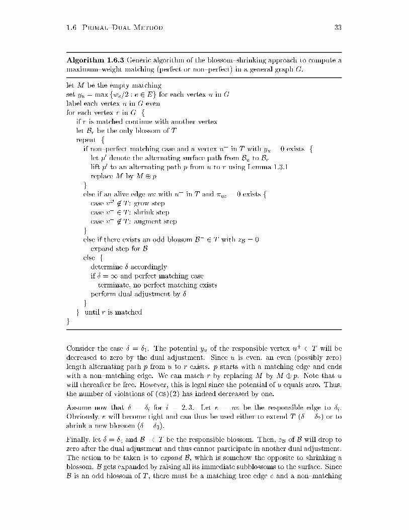
1.6 Primal{Dual Method 33Algorithm 1.6.3 Generi algorithm of the blossom{shrinking approa h to ompute amaximum{weight mat hing (perfe t or non{perfe t) in a general graph G.let M be the empty mat hingset yu = max fwe=2 : e 2 Eg for ea h vertex u in Glabel ea h vertex u in G evenfor ea h vertex r in G fif r is mat hed ontinue with another vertexlet Br be the only blossom of Trepeat fif non{perfe t mat hing ase and a vertex u+ in T with yu = 0 exists flet p0 denote the alternating surfa e path from Bu to Brlift p0 to an alternating path p from u to r using Lemma 1.3.1repla e M by M � pgelse if an alive edge uv with u+ in T and �uv = 0 exists f ase v? 62 T : grow step ase v+ 2 T : shrink step ase v+ 62 T : augment stepgelse if there exists an odd blossom B� 2 T with zB = 0expand step for Belse fdetermine Æ a ordinglyif Æ =1 and perfe t mat hing aseterminate, no perfe t mat hing existsperform dual adjustment by Ægg until r is mat hedgConsider the ase Æ = Æ1. The potential yu of the responsible vertex u+ 2 T will bede reased to zero by the dual adjustment. Sin e u is even, an even (possibly zero)length alternating path p from u to r exists. p starts with a mat hing edge and endswith a non{mat hing edge. We an mat h r by repla ing M by M � p. Note that uwill thereafter be free. However, this is legal sin e the potential of u equals zero. Thus,the number of violations of ( s)(2) has indeed de reased by one.Assume now that Æ = Æi for i = 2; 3. Let e = uv be the responsible edge to Æi.Obviously, e will be ome tight and an thus be used either to extend T (Æ = Æ2) or toshrink a new blossom (Æ = Æ3).Finally, let Æ = Æ4 and B� 2 T be the responsible blossom. Then, zB of B will drop tozero after the dual adjustment and thus annot parti ipate in another dual adjustment.The a tion to be taken is to expand B, whi h is somehow the opposite to shrinking ablossom. B gets expanded by raising all its immediate subblossoms to the surfa e. Sin eB is an odd blossom of T , there must be a mat hing tree edge e and a non{mat hing

34 Chapter 1. Mat hing Theorytree edge e0 in ident to B. Let b and d denote the endpoint of e and e0 that is ontainedin B. There must exists an even length alternating path p from Bd to Bb, the immediatesubblossoms of B ontaining d and b, lying ex lusively in (B). Moreover, all edges inp are tight. We add p and thus all immediate subblossoms lying on p to T and labelthem a ording to their even or odd length distan e to the root blossom Br of T . Allother immediate subblossoms of B not lying on p get unlabeled and leave the tree T .In Figure 1.5 an example is given of a so{ alled expand step.Obviously, (i7) holds whenever Æ = Æi, with i = 2; 3. Moreover, note that Æ = Æ1 willhappen at most on e per sear h and the o urren es of Æ = Æ4 during a sear h arebounded by O(n).10 Finally, when the potentials are adjusted in the way stated above,(i8) ertainly holds.Let us brie y onsider the di�eren es for the maximum{weight perfe t mat hing ase.The initial solutions onstru ted above will ertainly validate (j1) to (j4). Moreover,the details to mat h a free vertex using only tight edges stay the same. Moreover, thestated dual adjustment will assure invariants (j5) to (j7). The only di�eren e is thatthe potentials of even tree verti es are no longer restri ted to being non{negative. Asa onsequen e, Æ is not bounded above by Æ1. Therefore, hoosingÆ = minfÆ2; Æ3; Æ4gyields the desired result for the maximum{weight perfe t mat hing problem. Note thatÆ = 1 might in fa t happen in the perfe t ase, whereas this is prevented by theexisten e of Æ1 in the non{perfe t ase.Finally, we summarize Edmonds' blossom{shrinking approa h to �nd a maximum{weight mat hing (perfe t or non{perfe t) in a general graph by the generi algorithmdepi ted in Algorithm 1.6.3.1.6.4 Half{Integrality of the Dual SolutionWe will use this se tion to prove an important property of the dual solution onstru tedby the approa h des ribed in the pre eding se tion.Lemma 1.6.1 Let (y; z) be an optimal solution to (wm), where all edge weights areintegral. Then (y; z) is half{integral, or more pre isely:yu � 0 (mod 12) for all u 2 V , and (1)zB � 0 (mod 1) for all B 2 O. (2)Proof:Assume the algorithm starts with the initial solution (y; z) as des ribed above, i.e. yu =max fwe=2 : e 2 Eg for ea h vertex u and zB = 0 for all non{singleton odd ardinalitysets B. When we is integral for ea h edge e, (1) and (2) hold.10Observe that on e a blossom be omes an even tree blossom, it will stay even labeled and in T forthe rest of the sear h.

1.6 Primal{Dual Method 35Let (y; z) be a dual solution satisfying (1) and (2). Consider a dual adjustment byÆ > 0 and let (y0; z0) be the resulting dual solution. (1) and (2) will remain true for(y0; z0) when Æ an be proved to be half{integral. Æ is obviously half{integral whenÆ = Æ1 or Æ = Æ4 (a tually, Æ is integral i� Æ = Æ4). The redu ed ost �uv of an edgeuv is guaranteed to be half{integral by de�nition and (1) and (2). Thus Æ = Æ2 ishalf{integral. Finally, onsider the ase Æ = Æ3. We will show that the redu ed ost�uv of an edge uv with u+ 2 T and v+ 2 T must be integral. To see this, note that alledges e = uv in T are tight and all edge weights are integral. Thus, for these edges wehave: yu + yv + XB2Ouv2 (B) zB = wuvwhi h implies that yu + yv � 0 (mod 1) must hold for any two verti es u and v inT . Thus we an infer that the redu ed ost �uv of the edge uv is integral, and this on ludes the proof. �One an immediately aÆrm the following orollary for the maximum{weight perfe tmat hing ase.Corollary 1.6.1 Let (y; z) be an optimal solution to (wpm), where all edge weightsare integral. Then (y; z) is half{integral.1.6.5 Using the Alternative LP Formulation | Algorithmi Conse-quen esAs was mentioned above, the details of the primal{dual method we have developeddepend on the underlying linear programming formulation. Using the alternative linearprogramming formulation (wpm*) introdu ed in Se tion 1.4.3 one may hope to obtaina di�erent approa h for the maximum{weight perfe t mat hing problem | whi h ouldbe implemented more eÆ iently.The di�eren es of a primal{dual method based on the linear programming formulation(wpm*) are the subje t of this se tion.(wpm*) maximize wTxsubje t to x(Æ(u)) = 1 for all u 2 V , (1)x(Æ(B)) � 1 for all B 2 O, (2)xe � 0 for all e 2 E. (3)The dual linear program (wpm*) to (wpm*) is given below.(wpm*) minimize Xu2V yu + XB2O zBsubje t to zB � 0 for all B 2 O. (1)yu + yv + XB2Ouv2Æ(B) zB � wuv for all uv 2 E, (2)

36 Chapter 1. Mat hing TheoryNote that the redu ed ost �uv of an edge uv with respe t to a dual solution (y; z) isnow de�ned di�erently: �uv = yu + yv � wuv + XB2Ouv2Æ(B) zBThe omplementary sla kness onditions are thus:(p s*) xuv > 0 =) �uv = 0 for all edges uv 2 E, (1)zB > 0 =) x(Æ(B)) = 1 for all B 2 O. (2)All details of the primal{dual method for the weighted perfe t mat hing ase apply.However, the dual adjustment is performed di�erently in order to assure (j5) to (j7).The potentials are adjusted for surfa e blossoms (trivial or non{trivial) only.y0v = yv � Æ for all v+ 2 T ;y0v = yv + Æ for all v� 2 T ;y0v = yv for all vf?j+g 62 T ;z0B = zB � Æ for all B+ 2 T ;z0B = zB + Æ for all B� 2 T ;z0B = zB for all Bf?j+g 62 T :It seems one an implement the dual adjustment stated above more eÆ iently sin eonly surfa e blossoms have to be onsidered. However, the rux of using the linearprogramming formulation (wpm*) is the omputation of the redu ed ost of an edge.During the ourse of Algorithm 1.6.3 the redu ed ost �uv of alive edges uv will haveto be omputed frequently. Using the approa h dis ussed in the pre eding se tion,this an be a hieved by taking the potentials of u and v and the edge weight wuv into onsideration.11 In the approa h just sket hed, one would additionally have to takeinto onsideration all potentials zB of blossoms B with uv 2 Æ(B).1.7 Survey of Di�erent RealizationsOver the last four de ades various polynomial{time realizations of the blossom{shrinking approa h dis ussed in Se tion 1.6.3 have evolved. The �rst was suggestedby Edmonds himself as early as 1965. Its theoreti al running{time was bounded byO(n2m). Permanent improvements regarding the theoreti al running{time have beena hieved su essively using di�erent strategies and data stru tures. The urrent bestand optimal approa h for general edge weights has a running{time of O(n(m+n logn))and is due to Gabow [Gab90℄. We wish to use this se tion to portray the main ideasbehind four di�erent polynomial{time realizations of the blossom{shrinking approa h.One an view the blossom{shrinking approa h as working in phases. A phase terminateswhen an additional violation has been eliminated, i.e. a violation of ( s)(2) in the11Remember that alive edges are not ontained in any blossom and hen e PB2Ouv2 (B) zB = 0:

1.7 Survey of Different Realizations 37maximum{weight mat hing and a violation of (wpm)(1) in the maximum{weight per-fe t mat hing ase. Sin e at most n violations exist, where n denotes the number ofverti es in G, we have O(n) phases. Next, we will argue that the number of dualadjustments per phase is bounded by O(n). Therefore, observe that Æ = Æ1 o urs atmost on e in a phase. When Æ = Æi, with i = 2; 3, at least one (formerly non{evenlabeled) vertex be omes an even tree vertex. When a vertex has be ome an even treevertex it will stay even and reside in the tree until the end of the phase. Thus Æ = Æi,i = 2; 3, o urs O(n) times. Finally, whenever Æ = Æ4, a blossom gets expanded. Sin e ablossom annot ontain more than n verti es this will also happen at most O(n) times.A non{trivial part of the algorithm is to maintain the surfa e graph G. We sket h theidea of using a union{�nd data stru ture that additionally supports a split operation.Ea h vertex knows its surfa e blossom, e.g. by a pointer, and ea h surfa e blossommaintains a list of all its verti es. Identifying the surfa e blossom of a vertex thus takestime O(1). Two blossom Bi and Bj are united by size. That is, w.l.o.g. let jBij > jBj j.The pointer of ea h vertex in Bj is set to Bi, the list of Bj is appended to Bi and Bjis destroyed. Bi then represents the new blossom. Split operations, too, are done bysize. The list of a surfa e blossom Bi is split into two lists Bi and Bj. Again, the largerblossom, say Bi, is reused and ea h pointer of a vertex in the smaller blossom is setto Bj. By always resetting the pointers of the smaller blossom, we an assure thatea h �xed vertex ontributes no more than O(log n) time to a series of n union or splitoperations. Note, however, that the laimed time bound only holds for a series of splitfollowed by a series of union operations, or vi e versa; and not for an arbitrary orderof intermixed union and split operations. But sin e a vertex an parti ipate in a seriesof at most O(n) split (expand steps) followed by a series of O(n) union (shrink steps)operations, a total time of O(n logn) per phase results. This will be suÆ ient for allfour realizations presented next.The realizations di�er in the way they �nd tight edges, determine the value of Æ andperform a dual adjustment.1.7.1 An O(n2m) Approa hA simple realization needs time O(m) to �nd tight edges and to determine the valueof Æ (ea h edge is inspe ted on e). Performing a dual adjustment an be a hievedby expli itly updating the potential of ea h vertex and non{trivial surfa e blossomwhi h takes time O(n). The total running{time is thus O(n2(n +m)) = O(n2m) orO(n4), sin e m is bounded above by n2. This approa h is essentially the one whi h wassuggested �rst by Edmonds [Edm65a℄.1.7.2 An O(n3) Approa hThe only parts that need more than O(n) time per dual adjustment in the aboverealization are the identi� ation of tight edges and the determination of Æ, or, to bemore pre ise, the determination of Æ2 and Æ3.12 As we shall see, either an be a hieved12Obviously, the determination of Æ1 and Æ4 an easily be a hieved in time O(n).

38 Chapter 1. Mat hing Theoryin time O(n). The resulting O(n3) approa h is due to Lawler [Law76℄.We say an alive edge e in ident to a surfa e blossom B (trivial or non{trivial) is a bestedge of B when its redu ed ost is minimal, i.e.�e = min f�uv : uv 2 Æ(B) and uv is aliveg:When several su h edges exist for B, the best edge of B refers to an arbitrary one ofthese.To handle Æ2, ea h vertex uf?j+g 62 T stores its best edge uv from u to an even labeledtree vertex v+ 2 T . Moreover, u stores the redu ed ost �uv of its best edge. Sin e oddverti es might leave T and get unlabeled (due to an expand step), the same data mustbe available for ea h odd tree vertex u� 2 T . Finding tight edges and determining Æ2 an then be a hieved in time O(n) by inspe ting ea h best edge of uf?j+g 62 T verti es.A dual adjustment is performed by updating the redu ed ost of all best edges ofuf?j+g 62 T verti es whi h takes at most O(n) time.Ea h surfa e blossom B+k 2 T stores for ea h adja ent surfa e blossom B+j 2 T , withBk 6= Bj, the best edge ekj = uv with u 2 Bk and v 2 Bj. Moreover, Bk knows theredu ed ost �ek of the best edge ek of all best edges ekj. Finding tight edges is a hievedby inspe ting all best edges of the blossom whose best edge has redu ed ost zero. Thetime needed to do so is bounded by O(n). By exploring the redu ed ost �ek of thebest edge ek to ea h blossom B+k 2 T , Æ3 an be determined in time O(n). Adjustingthe redu ed ost �ek of ea h blossom B+k 2 T needs time O(n).p qIt remains to be shown, however, that the information asso iated with the maintenan e of Æ2and Æ3 an be kept orre t without using time more than O(n2) per phase. Whenever a vertexbe omes an even tree vertex, its edges are s anned and the information for Æ2 and Æ3 is updated.When a new blossom Bk is formed by s immediate subblossoms, it takes time O(sn) to set upthe data for Bk.13 The total ost T (n) per phase to maintain Æ3 an then be omputed by thefollowing re ursion: T (n) = O(sn) + T (n� s). By indu tion it follows that T (n) equals O(n2).Sin e ea h edge is s anned at most twi e in a phase (on e from ea h endpoint) this ontributestime O(m) per phase. Altogether, the approa h needs time O(n(n2 +m)) = O(n3).x yFinally, observe that the idea of maintaining the best (alive) edge to ea h pair of evensurfa e blossoms gives a lower bound of (n2) per phase.1.7.3 An O(nm logn) Approa hAnother realization, whi h improves the theoreti al running{time to O(nm logn), isdue to Galil, Mi ali and Gabow [GMG86℄. This approa h is superior to the O(n3)13We give details to derive the laimed time bound. Let B�i , 1 � i � bs=2 , denote the immediateodd subblossoms of Bk. Ea h Bi, 1 � i � bs=2 is made even. All edges of the verti es ontained inBi, 1 � i � bs=2 , are s anned to update the information for Æ2 and to determine the best edges eijof Bi to other even tree blossoms B+j 2 T . Thereafter, the best edges ekj and the redu ed ost of thebest edge ek of all best edges of Bk an be determined in time O(sn). We have to update the best edgeinformation of ea h blossom B+j 2 T adja ent to the new blossom Bk. This will need time O(sn). Tosee this, onsider a �xed blossom B+j 2 T that is adja ent to Bk. Deleting all best edges eji to an evensubblossom B+i 2 T of Bk takes time O(s). Updating the best edge ejk to Bj takes time O(1). Sin ethe number of adja ent blossoms is bounded by n the total time of O(sn) results.

1.7 Survey of Different Realizations 39approa h for sparse graphs. More or less the same ideas as in the O(n3) approa h arereused. However, priority queues will help to a hieve an O(m log n) time bound perphase. We will not go into detail here but postpone the dis ussion to Chapter 2. Onlya few di�eren es are outlined.For example, Æ3 will be maintained by a priority queue. At �rst glan e the usage ofpriority queues does not seem to work, due to the frequent hanges of the priorities aftera dual adjustment. Taking advantage of the fa t that all priorities hange uniformlywill help to ir umvent this problem in an eÆ ient way.Another major di�eren e to the O(n3) approa h is that we abandon the goal of onlykeeping tra k of the alive edges between even tree blossoms. Instead, a lazy deletionstrategy is used to maintain Æ3. That is, every alive edge that might be of interest forÆ3 is inserted into Æ3. As a onsequen e, after a series of shrinkings, Æ3 might ontainedges that are no longer alive. These edges are deleted when they are en ountered asthe minimal element of Æ3. A tually, this will be the only point where the running{timeof O(m+ n log n) per phase is ex eeded.For the sake of ompleteness we state the theoreti al running{time for �nding tightedges, for determining Æ and for performing a dual adjustment. Finding a new tightedge will orrespond to a delete min operation on a priority queue and thus takes, atmost, time O(log n). The same will hold for the determination of Æ. To perform adual adjustment, however, will only take time O(1) and is thus an immense speed{up ompared to the O(n3) approa h.1.7.4 An O(n(m+ n logn)) Approa hIn 1990, Gabow [Gab90℄ presented a data stru ture that an be used to realize a phaseof Edmonds' blossom{shrinking approa h in theoreti al running{time O(m + n logn).Gabow laimes this time bound to be optimal: sorting n numbers an be redu ed toa sear h for an augmenting path in Edmonds' blossom{shrinking approa h; originally,a similar argument was given by Fredman and Tarjan [FT87℄ to prove optimality ofDijkstra's algorithm. Sin e ea h edge may be onsidered on e during a sear h, a lowerbound of (m+ n logn) per phase results.The details of the approa h are omplex and will not be given here. We attempt tosket h the idea, although this is diÆ ult without going into detail. As mentioned before,only the maintenan e of Æ3 needs spe ial re�nement. Therefore, a kind of alternatingtree T is grown. Ea h blossom forming edge uv (i.e. the edge uv with u+ 2 T andv+ 2 T ) is repla ed by two (dire ted) ba k edges ul and vl, where l denotes the lowest ommon an estor of u and v in T . A shrink operation then orresponds to unitingall surfa e blossoms along the y le C1 = (l; : : : ; u; l) and C2 = (l; : : : ; v; l). Theseba k edges are further partitioned into log n sets alled pa kets. Roughly speaking, bydealing with the pa kets' minima (in terms of redu ed ost) the desired time bound anbe a hieved.However, the underlying data stru tures are omplex and we doubt that an implemen-tation would be eÆ ient in pra ti e.

Chapter 2O(nm logn) Approa hThe demanding and ostly parts in Edmonds' blossom{shrinking approa h are the per-forming of dual adjustments and the determination of the value of Æ (see Se tion 1.6.3).In 1986, Galil, Mi ali, and Gabow [GMG86℄ presented a strategy that enables a phaseof Edmonds' blossom{shrinking approa h to be realized in time O(m log n). The timebound is a hieved by using a sophisti ated data stru ture, whi h they all generalizedpriority queues. Generalized priority queues support all standard priority queue opera-tions. Additionally, the priorities of ertain subgroups of elements in the queue an beuniformly hanged by a single operation.The ideas we will develop in this hapter are similar to or have been developed fromthe ideas of Galil et al. However, our approa h di�ers with regard to the maintenan eof the varying priorities. Galil et al. handle these hanges within the priority queuedata stru ture, whereas we will establish a series of formulae that enable us to omputethese priorities as needed.First, we shall illustrate how the blossom potentials and redu ed osts of edges anbe omputed after a series of dual adjustments. As a onsequen e, the time requiredto perform a dual adjustment will be redu ed to O(1). Next, the on ept of usingpriority queues to determine the value Æ and thus also the responsible vertex, edge orblossom will be onsidered more losely. Finally, an obvious but mistaken realizationwill motivate the appli ation of on atenable priority queues.2.1 Varying Potentials and Redu ed CostsThe frequent modi� ations of the blossom potentials and, onsequently, the redu ed ost of edges aused by a dual adjustment make it diÆ ult to realize a phase in theblossom{shrinking approa h eÆ iently. However, the a onsiderable advantage is thatthese modi� ations o ur in a uniform manner. In the subsequent se tions we willillustrate how to take advantage of that fa t.

41

42 Chapter 2. O(nm log n) Approa h2.1.1 Potential UpdateConsider a dual adjustment that is performed during the ourse of Algorithm 1.6.3 (de-s ribed in Se tion 1.6.3). Let T denote the urrent alternating tree. A dual adjustmentby Æ a�e ts the potentials of all verti es and non{trivial surfa e blossoms as follows.The vertex potential hanges by �Æ for an even tree vertex u+ 2 T , by +Æ for an oddtree vertex u� 2 T and by 0 for an non{tree vertex uf?j+g 62 T . Correspondingly, thepotential of a non{trivial surfa e blossom is adjusted by +2Æ for an even tree blossomB+ 2 T , by �2� for an odd tree blossom B� 2 T and by 0 for a non{tree blossomBf?j+g 62 T .Therefore, after a series Æ1; Æ2; : : : ; Æk of dual adjustments the so{ alled a tual potentialof a vertex or non{trivial surfa e blossom an be omputed by taking its initial potential,its status and the value of � = Pki=1 Æi into onsideration. The status of a blossom(trivial or non{trivial) is given by its label and the property of either being a tree or anon{tree blossom.More pre isely, as long as the status of a vertex u does not hange it is possible toobtain its a tual potential eyu from its initial potential yu by the following formula:eyu = yu + ��:Similarly, on the assumption that the status of a non{trivial surfa e blossom B isinvariant, the a tual potential ezB an be omputed via its initial potential zB:ezB = zB � 2��:The oeÆ ient � depends on the urrent status of a blossom B (trivial or non{trivial)and will be alled the status indi ator:� = 8><>: �1 when B+ 2 T ,1 when B� 2 T , and0 when Bf?j+g 62 T .However, the status of a blossom hanges during the ourse of the algorithm and theformulae given above are somewhat oversimpli�ed. We next re�ne these formulae su hthat arbitrary status hanges an be handled as well.Consider �rst of all a status hange for a vertex u. Let �1 and �2 denote the sum ofdual adjustments before and after the status hange and assume u hanges its statusindi ator from � to �0. Then,eyu = yu + ��1 + �0�2 �=�1+�2= yu + (� � �0)�1 + �0�:That is, we need to orre t the potential yu by +(� � �0)� at the point of time whenu hanges its status indi ator from � to �0 (and thus � = �1).Analogously, let us onsider a status hange for a non{trivial surfa e blossom B. It isezB = zB � 2��1 � 2�0�2 = zB � 2(� � �0)�1 � 2�0�

2.1 Varying Potentials and Redu ed Costs 43and therefore the potential zB is orre ted by �2(� � �0)� when the urrent statusindi ator � of B hanges to �0. Again, at this point � will equal �1.As will be ome lear shortly, we annot a�ord to orre t the potential of ea h ver-tex ontained in a non{trivial surfa e blossom separately. Observe, however, that the orre tion value of a vertex potential and that of the non{trivial surfa e blossom on-taining that vertex di�ers by a multipli ative fa tor of �2. We an therefore simulatethe potential orre tions by means of an o�set assigned to ea h surfa e blossom, asdes ribed next.Ea h surfa e blossom B (trivial or non{trivial) has an o�set denoted by o�setB. Thea tual potential of a vertex u is then omputed byeyu = yu + o�setB + ��; (2.1)where B orresponds to the surfa e blossom ontaining u (trivial or non{trivial). A - ordingly, the a tual potential of a non{trivial surfa e blossom B an be obtained byezB = zB � 2o�setB � 2��: (2.2)A status hange for a surfa e blossom B then redu es to an update of its o�set value:o�setB = o�setB + (� � �0)�; (2.3)where � denotes the sum of dual adjustments up to the time of the status hange.During the ourse of the algorithm, the o�set of a surfa e blossom B is adjusted asin (2.3) whenever its status hanges. The dis ussion of how to handle the o�sets in ashrink or an expand step is postponed to the next but one se tion.2.1.2 Maintenan e of Redu ed CostsFor ea h vertex uf?j+g 62 T and u� 2 T we will need to keep tra k of the best edge uvto an even labeled tree vertex and the redu ed ost �uv of that edge. We will do so byassigning a pair (�uv; uv) to ea h su h vertex, where uv denotes an edge in ident to u,with v+ 2 T , having redu ed ost �uv.In the ontext of this hapter it would be suÆ ient to handle only one su h pair pervertex. However, we will onsider a more general ase where ea h vertex u is asso iatedwith a series (�uv1 ; uv1); (�uv2 ; uv2); : : : ; (�uvk ; uvk) of pairs. Ea h pair (�uvi ; uvi) keepsan edge uvi in ident to u, with v+i 2 T , and the redu ed ost �uvi of that edge.This extended view will turn out to be reasonable in Chapter 3 (Se tion 3.4), wherevarious alternating trees are simultaneously grown and hen e several edges and theirredu ed osts will be asso iated with any vertex, i.e. also with even labeled tree verti es.In the subsequent se tions, we will expli itly mention when the results apply to theextended view only.The redu ed osts of all edges asso iated with a vertex u may vary with dual adjust-ments. As for the blossom potentials, we will elaborate a formula whi h enables thea tual redu ed osts of these edges to be omputed.

44 Chapter 2. O(nm log n) Approa hFor a vertex u+ 2 T , u� 2 T or uf?j+g 62 T , a dual adjustment by Æ hanges the redu ed osts of all edges asso iated with u uniformly by �2Æ, 0 or �Æ, a ordingly. Therefore,as long as u does not hange its status, we an again ompute the a tual redu ed oste�uvi of an edge uvi after a series of dual adjustments taking its initial redu ed ost, thestatus of u and the total dual adjustment value � into onsideration. The omputationformula an even be expressed by means of u's status indi ator � as introdu ed in thepre eding se tion: e�uvi = �uvi + (� � 1)�:Let us, on e again, onsider the value by whi h the redu ed ost �uvi has to be orre ted,when u hanges its status indi ator from � to �0. As before, �1 and �2 denote thesum of dual adjustments that have been performed before and after the status hange:e�uvi = �uvi + (� � 1)�1 + (�0 � 1)�2 = �uvi + (� � �0)�1 + (�0 � 1)�:Thus, we would have to in rease the redu ed ost �uvi of ea h edge uvi by (� � �0)�whenever u hanges its status. Observe that the o�set of the surfa e blossom B on-taining u is in reased by exa tly this amount, and we an therefore attain the sameresult by omputing the a tual redu ed ost with respe t to that o�set also:e�uvi = �uvi + o�setB + (� � 1)�: (2.4)Thus, we postulate that the a tual redu ed ost e�uvi of any edge uvi asso iated with uis omputed by Formula (2.4).One �nal remark must be made here. Imagine that at some point of time a new edgeuvk+1 having a tual redu ed ost e�uvk+1 is to be added to u. The redu ed ost �uvk+1that is a tually stored with the new pair (�uvk+1 ; uvk+1) of u must then equal�uvk+1 = e�uvk+1 � o�setB � (� � 1)�: (2.5)We will therefore all �uvk+1 the stored redu ed ost of the edge uvk+1, also.2.1.3 Managing the Blossom O�setsIn the pre eding two se tions several formulae have been developed to ompute boththe a tual potential of a blossom and the a tual redu ed ost of edges asso iated witha vertex. In either ase, the value of interest is obtained by taking the o�set of thesurfa e blossom into onsideration. What remains to be shown is how one an handlethese o�sets when a shrink or an expand step o urs.Managing the Blossom O�sets | Shrink StepLet B, with (immediate) subblossoms B1;B2; : : : ;B2k+1, denote the blossom to beformed. Ea h odd labeled subblossom Bi is made even by adjusting its o�set as previ-ously des ribed (see (2.3)). The o�sets o�setB1 ; o�setB2 ; : : : ; o�setB2k+1 may di�er invalue. However, we want to a hieve a situation where the a tual potential and also the

2.1 Varying Potentials and Redu ed Costs 45a tual redu ed osts asso iated with ea h vertex u 2 Bi an be omputed with respe tto the new surfa e blossom o�set o�setB.The following strategy assures that the o�sets of all (immediate) subblossoms Bi, 1 �i � 2k + 1, are equally set to zero. The a tual potential and redu ed osts asso iatedwith any vertex ontained in the new blossom B an thus be omputed with respe t tothe o�set o�setB = 0.When a surfa e blossom B0 (trivial or non{trivial) be omes an even tree blossom forthe �rst time during a phase, its o�set o�setB0 is set to zero. Thus, in order to preservethe validity of (2.1) and (2.2) for the omputation of the a tual potential eyu of ea hvertex u 2 B0 and of the a tual potential ezB0 of B0 itself (when B0 is non{trivial only),the following adjustments have to be performed:yu = yu + o�setB0 , andzB0 = zB0 � 2o�setB0 :In the extended view mentioned in the pre eding se tion, even tree verti es are alsoasso iated with a series of pairs. In this ase, the stored redu ed ost �uv of ea h su hpair (�uv; uv) asso iated with u is subje t to orre tion:�uv = �uv + o�setB0 :We wish to emphasize that the des ribed updates are performed for every blossom thatbe omes an even tree blossom (an even tree blossom need not ne essarily parti ipatein a shrink step). We thus de ided to all this strategy the provident strategy.Observe that the adjustments are performed at most on e for a �xed vertex per phase.Thus, the time required for the potential adjustments is O(n) per phase. The orre tionof the redu ed osts ontributes time O(mtadj) per phase, where tadj denotes the timeneeded by the operation to hange the stored redu ed ost.1 We will keep the pairsasso iated with a vertex in a priority queue (as will be explained in Se tion 3.4) andthus tadj is bounded by O(log n). In summary, a total time bound of O(n +m logn)per phase results.p qWe wish to present another strategy, in whi h the new o�set o�setB is determined by the o�setvalue o�set� of the (immediate) subblossom Bi that survives in the following pro edure.We iterate over all (immediate) subblossoms of B. Initially, o�set� is set to the o�set of B1.In ea h stage i, 1 � i � 2k, the a tual potential of ea h vertex ontained in a subblossomBj with j � i is omputed with regard to the o�set o�set�. Let i = Pij=1 jBj j denote thetotal number of these verti es. We use i+1 to denote the number of verti es ontained in thesubblossom Bi+1. When i � i+1, o�set� survives and all verti es of Bi+1 lose; otherwiseo�setBi+1 survives and all verti es of the Bj 's lose. o�set� is set to the survivor o�set and theother o�set is denoted by o�set l (the a tual potentials of all loser verti es are omputed withrespe t to that o�set). The potentials yu of all loser verti es u are adjusted su h that theira tual potentials are omputed orre tly with respe t to the o�set o�set�, i.e.yu = yu + o�set l � o�set�:1The total number of pairs stored for all verti es will be bounded by O(m).

46 Chapter 2. O(nm log n) Approa hAs before, it is only in the extended view (where not only unlabeled and odd labeled verti esbut also even tree verti es are asso iated with a series of pairs) that the stored redu ed ost�uv of ea h su h pair (�uv ; uv) needs to be adjusted:�uv = �uv + o�set l � o�set�:We do not adjust the potentials zBi of the non{trivial subblossoms Bi here, sin e they in any ase require a spe ial treatment, as will be des ribed below. We all this strategy the non{provident strategy, sin e the ne essary adjustments are performed on demand, i.e. when the orresponding vertex in fa t parti ipates in a shrink step.Let us pro eed to the determination of the time needed by these adjustments. Sin e we alwaysadjust the potentials and stored redu ed osts of losing verti es only, the ne essary adjustmentsfor a �xed vertex u will be performed at most O(logn) times per phase.2 The ost for updatingthe potential of u is O(1). Moreover, sin e the number of edges asso iated with u will beno greater than its degree deg(u), the time required to adjust the stored redu ed osts isO(deg(u) tadj), where tadj denotes (as above) the time needed by the operation to hange thestored redu ed ost. We on lude that ea h vertex u ontributes O((1 + deg(u) tadj) logn) timeper phase. As mentioned previously, tadj is bounded by O(logn). Thus, summing over allverti es we obtain a total time bound of O((n + m logn) logn) = O(n logn + m(logn)2) perphase. That is, the theoreti al time bound of O(m logn) per phase is ex eeded. In pra ti e,however, the non{provident strategy turned out to be slightly more eÆ ient than the providentstrategy (as will be presented in Se tion 3.6). It therefore seems to us that this strategy isworth being onsidered.3 Our multiple sear h tree implementation (dis ussed in Se tion 3.4)implements both the provident and the non{provident strategy.x yAfter the new blossom B has been formed, the a tual potential ezBi of ea h non{trivialsubblossom Bi is no longer a�e ted by future dual adjustments. We therefore freeze thepotential of these blossoms by adopting the following onvention. For any non{trivialsubblossom Bi, we ensure that the potential zBi equals its a tual potential ezBi . Thus,at the time of shrinking we set:zBi = zBi � 2o�setBi � 2��;and sin e every subblossom of B has been made even before, the above equation redu esto zBi = zBi � 2o�setBi + 2�:The time needed to perform these potential freezings is proportional to the number ofnon{trivial subblossoms of B.2There are n verti es and after ea h adjustment for u, u will reside in a group of ardinality at leasttwi e as large as before.3Moreover, note that all stored redu ed osts of a �xed vertex u are adjusted by the same amount.Therefore, the underlying priority queue data stru ture, whi h organizes these redu ed osts, ould alsoimplement an operation, say hange all priorities, whi h hanges all priorities in the queue by the sameamount in time O(deg(u)). For example, assume the priority queue is realized by a balan ed binarytree (i.e. having height O(log(deg(u)))), where the items of the priority queue orrespond to the leavesof the tree. Then, traversing ea h vertex (i.e. non{leaf verti es too) of the tree and expli itly updatingthe stored priority of that vertex will take time proportional to deg(u). As a onsequen e, the totaltime needed by the non{provident strategy would be redu ed to O((n+m) log n) per phase, as desired.

2.2 Determination of Æ | towards a Priority Queue Approa h 47Managing the Blossom O�sets | Expand StepThe details for an expand step now ensue easily. Let B denote the odd surfa e blossomthat is going to be expanded. As for the shrink step, the (immediate) subblossoms ofB are denoted by B1;B2; : : : ;B2k+1. The a tual potential and the a tual redu ed ostsasso iated with ea h vertex ontained in B an be omputed by the formulae establishedabove; these values depend on the o�set o�setB of B, whi h is therefore assigned to ea hof the subblossom o�sets, i.e. o�setBi = o�setB. Moreover, ea h subblossom be omesodd labeled and the potential zBi of all non{trivial subblossoms Bi undergo unfreezingwith respe t to the new o�set:zBi = zBi + 2o�setBi � 2��whi h equals zBi = zBi + 2o�setBi � 2�sin e ea h Bi is labeled odd. Obviously, the time required to unfreeze the blossompotentials is proportional to the number of non{trivial subblossoms of B. Afterwards,the ne essary status hanges for some of the subblossoms Bi, for instan e for thosethat leave T , an be handled by an o�set adjustment as dis ussed above (see Equation(2.3)).Summarizing, we have established a onvenient way to handle the varying blossompotentials as well as the redu ed osts of edges asso iated with a vertex. The valueof interest an be omputed on demand by the formulae developed. Here, making ano�set available to ea h surfa e blossom and keeping tra k of the total amount � ofdual adjustments turned out to be the key ideas. The additional overhead produ ed bythe o�set maintenan e has been proved to onsume O(m log n) time per phase. A dualadjustment by Æ redu es to an in rease of � by Æ and an thus be performed in timeO(1).2.2 Determination of Æ | towards a Priority Queue Ap-proa hWe next onsider more losely the idea of using priority queues to determine the valueof Æ, and show how all priorities stored in a priority queue an be adjusted in a uniformmanner.Re all that Æ is hosen as the minimum of the four values Æ1; Æ2; Æ3 and Æ4 (see Se -tion 1.6.3). In order to determine ea h one of these we keep a orresponding priorityqueue delta1 , delta2 , delta3 and delta4 .4 The priorities in ea h of the priority queues hange with ea h dual adjustment and at �rst glan e there seems to be little hope thatthis approa h will turn out to be eÆ ient. However, an essential observation is that4We assume some familiarity with the priority queue data type. All standard operations, like insert,delete min, �nd min et , are assumed to take time no more than O(log n), where n denotes the numberof items stored in the priority queue. For a detailed dis ussion of these operations see, for example,Cormen et al. [CLR92℄.

48 Chapter 2. O(nm log n) Approa hone an arrange the priority queues su h that all priorities de rease uniformly by thedual adjustment value Æ. Consequently, the so{ alled a tual priority, denoted by ep,of any item in ea h of the priority queues an be omputed from its stored priority p,i.e. the priority whi h is stored with that item in the priority queue, and the total dualadjustment value � as de�ned above.More pre isely, we ensure that a priority p stored in any of these four priority queues orresponds to the a tual priority ep = p��. As a onsequen e, when a new item having(a tual) priority ep has to be inserted into one of the priority queues, the priority p whi his stored with that item is set to ep + �, where � denotes the total dual adjustmentsperformed up to this point. We next dis uss the semanti s of the items ontained inea h of the priority queues.delta1 onsists of all items hp; ui with u+ 2 T . The a tual priority p�� orrespondsto the a tual potential eyu of u.Ea h item hp; uvi in delta2 represents the best edge of a vertex vf?j+g 62 T to an evenlabeled tree vertex u+ 2 T . The a tual redu ed ost e�uv of this edge equals the a tualpriority p��.delta3 keeps tra k of the edges uv onne ting two even labeled tree verti es u+ 2 Tand v+ 2 T . The edges inserted into delta3 are ensured to be alive; however, duringthe ourse of the algorithm some of the edges stored in delta3 might be ome dead. Weuse a lazy{deletion strategy for these edges: dead edges are simply dis arded when theyo ur as the minimal item of delta3 . Ea h edge is represented by an item hp; uvi indelta3 . The a tual priority p�� orresponds to one half of the a tual redu ed ost ofuv, i.e. p�� = e�uv=2.The priority queue delta4 ontains for ea h odd labeled non{trivial surfa e blossomB� 2 T an item hp;Bi. The a tual priority p � � of this item is equal to one half ofthe a tual potential of B: p�� = ezB=2.p qWe brie y argue that all a tual priorities of delta1 , delta2 , delta3 and delta4 de rease by thedual adjustment value Æ. The potentials of all verti es u+ 2 T are de reased by Æ and thereforethe a tual priorities of delta1 de rease by Æ. Sin e only the potential of the endpoint u+ 2 Tfor all edges uv stored in delta2 is de reased by Æ, ea h a tual priority of delta2 de reases byÆ. For ea h edge uv stored in delta3 the potential of both endpoints is de reased by Æ. Thea tual priority of ea h edge is one half of the redu ed ost of that edge. Therefore, ea h a tualpriority de reases by Æ. Finally, the potential of ea h non{trivial surfa e blossom is redu ed by2Æ, and its a tual potential in delta4 thus de reases by Æ.x yLet us suppose that the priority queues delta1 , delta2 , delta3 and delta4 are maintained orre tly. Ea h value Æ1; Æ2; Æ3 and Æ4 an then be determined by a �nd min operationon delta1 , delta2 , delta3 and delta4 , respe tively. Moreover, �nding the responsiblevertex, edge or blossom redu es to a delete min operation on the priority queue fromwhi h Æ results. Summarizing, both the determination of Æ and also of the responsiblevertex, edge or blossom an be a hieved in time O(log n).55A omment is in order at this point. delta3 might ontain up to m items and thus an upper boundof O(logm) results. At �rst sight, it seems that the stated time bound of O(log n) is ex eeded; butnote that m � n2, and therefore O(logm) = O(log n).

2.3 A Misleading Strategy | Traps and Pitfalls 492.3 A Misleading Strategy | Traps and PitfallsHaving the outlined ideas in mind, it seems as if one ould immediately implementthe blossom{shrinking approa h that guarantees the stated time bound of O(m logn)per phase. However, the realization des ribed next will not fully omply with thestated time bound. The reasons for our de ision to present a mistaken realization aresubstantiated by the following three arguments. First, we have been misled by thisrealization ourselves. Se ond, it will serve as a basis that an easily be extended to a orre t approa h. And �nally, it will eventually provide us with an intuitive grasp su hthat we will aÆrm the need for on atenable priority queues.An alternating tree T is grown from a free vertex r as des ribed in Algorithm 1.6.3.Initially ea h vertex is a surfa e blossom having o�set value 0, and the value of � isset to 0. The initial potential stored with ea h vertex equals its a tual potential. Atthe beginning of a phase, ea h of the priority queues delta1 , delta2 , delta3 and delta4is made empty.For ea h vertex uf?j+g 62 T or u� 2 T we keep tra k of its best edge uv to an evenlabeled tree vertex and of the (stored) redu ed ost �uv of that edge by means of a pair(�uv; uv). Moreover, we adopt the onvention that a designated pair (1; ;) is assignedto u, when no su h edge has been en ountered during the urrent phase.Whenever a vertex u be omes an even tree vertex, its a tual potential eyu is omputedby (2.1) and a orresponding item heyu +�; ui is inserted into delta1 . We go throughall in ident edges uv of u in order to keep delta2 and delta3 orre t; this will ontributeO(m) time per phase, sin e ea h vertex that be omes an even tree vertex will stay evenand remain in T for the rest of the phase. When uv is dead or is a tree edge, it is simplydis arded. Otherwise, uv is alive and we an thus ompute its a tual redu ed ost:e�uv = eyu + eyv � wuv;where eyv is obtained by Formula (2.1) and wuv denotes the weight of that edge.6 Thea tion to be taken depends on the status of the endpoint v:Case 1: vf?j+g 62 TWe onsider only the ase where uv is the new best edge of v, sin e otherwisenothing has to be done.When (1; ;) is the pair stored with v, uv will be the new best edge to v andwe therefore repla e that pair by (�uv; uv), where the stored redu ed ost�uv is omputed by Formula (2.5). A new item he�uv +�; uvi is inserted intodelta2 .Otherwise, let (�uv; uv) denote the pair stored with v. We an ompute thea tual redu ed ost e�uv of uv by Equation (2.4). When e�uv < e�uv, uv will6Re all that the redu ed ost �uv of an edge uv has been de�ned as repeated below, where in the urrent ontext the potentials refer to the a tual potentials. Moreover, sin e uv is alive the sum overall blossom potentials ontaining that edge must equal 0.�uv = yu + yv � wuv + XB2Ouv2 (B) zB:

50 Chapter 2. O(nm log n) Approa hbe the new best edge of v. The pair stored with v is repla ed by (�uv; uv),where �uv refers to the stored redu ed ost (obtained by Equation (2.5)),and the item stored for v in delta2 is repla ed by he�uv +�; uvi.Case 2: v+ 2 TThe item he�uv=2 +�; uvi is simply inserted into delta3 .Case 3: v� 2 TThe same des ription as for vf?j+g 62 T applies, but no item is inserted orrepla ed in delta2 .When a non{tree blossom B enters T , ea h item in delta2 orresponding to a vertexu 2 B is deleted. Moreover, when B is non{trivial and be omes an odd tree blossom, we ompute its a tual potential ezB by (2.2) and insert the item hezB=2 +�;Bi into delta4 .When a vertex v� 2 T leaves T due to an expand step, we use the pair (�uv; uv) storedwith v in order to set up an item for delta2 ; if (1; ;) is assigned to v, we do nothing.The a tual redu ed ost e�uv of uv is omputed as in (2.4), and the item he�uv +�; uviis inserted into delta2 .Determining Æ, performing a dual adjustment and �nding the responsible vertex, edgeor blossom are a hieved as previously des ribed. All remaining details, e.g. shrinkingor expanding a blossom et ., follow easily from the dis ussion above.p qOne �nal remark is in order at this point. Sin e an unlabeled vertex might be ome an odd treevertex and then leave T again due to an expand step, one may wonder why it is suÆ ient tomaintain for ea h vertex v? 62 T and v� 2 T the best edge uv to a vertex u+ 2 T only. Note,however, that on e the best edge uv of a vertex v? 62 T has been used for a grow step, v willstay in T for the rest of the phase | even if all blossoms ontaining v are expanded during thatphase.x ySo far, it seems that the running{time of O(m log n) per phase has been a hieved.Observe, however, that ea h vertex entering or leaving T auses a deletion or insertionon delta2 . In the rest of this se tion we will justify in detail the laim that it is due tothe expansion of blossoms that these insertions and deletions may be exe uted up toO(n2) times and thus ex eed the laimed time bound.Readers who are not interested in these details are advised to skip to Se tion 2.4.2.3.1 Maximum Height of a Blossom Treep qFirst, we need to introdu e the on ept of a so{ alled blossom tree, whi h represents the nestingof a blossom B.Let B be a blossom. Ea h subblossom Bi � B orresponds to a node ui in the blossom tree BTBof B.7 The root node u of BTB stands for the blossom B itself. Consider a node ui in BTB that orresponds to a subblossom Bi � B. The hildren of ui in BTB are the nodes ui1 ; ui2 ; : : : ; uik ,where ea h uij , 1 � j � k, orresponds to an immediate subblossom Bj of Bi (see Figure 2.1for an example). From the onstru tion of BTB it follows that the verti es ontained in B orrespond to the leaves of BTB.7In order to avoid onfusion, we will use the term node when referring to verti es in the blossomtree.

2.3 A Misleading Strategy | Traps and Pitfalls 51B

(a)BTB

(b)Figure 2.1: Let B be a blossom whose nesting stru ture is given in (a). The blossom treeBTB of B is formed as depi ted in (b). In BTB, the root node stands for B, ea h internal(i.e. non{leaf) node represents a non{trivial subblossom of B and every leaf orresponds to avertex of B.The ardinality p of a blossom B is de�ned as the number of verti es ontained in B. Further-more, a blossom is said to be of size s, when it ontains s immediate subblossoms.Lemma 2.3.1 Let B be a blossom of ardinality p and BTB the orresponding blossom tree.The height h of BTB is bounded by O(p).Proof:Let Lh denote the number of leaves in a blossom tree of height h. We have L0 = 1, sin e ablossom tree of height zero represents a trivial blossom. A blossom tree of height one has atleast three leaves: L1 � 3.Generally speaking, a blossom tree of height h has Lh � Lh�1 + 2 leaves. The re ursion aneasily be solved:Lh � Lh�1 + 2 � Lh�2 + 2 + 2 � : : : � L0 + 2 + : : :+ 2| {z }h times = 2h+ 1Sin e the number of leaves in BTB orresponds to the ardinality p of B, we obtain:h � (p� 1)=2. �Lemma 2.3.1 implies that the height of a blossom tree BTB to a blossom B having maximum ardinality may be O(n).In Se tion 1.6.5, the disadvantage of omputing the redu ed ost of an edge using the alter-native linear programming formulation of the maximum{weight perfe t mat hing problem was

52 Chapter 2. O(nm log n) Approa houtlined.8 Using the terms introdu ed above, the time required to ompute the redu ed ostof an edge uv onne ting the blossoms Bu and Bv is proportional to the height of the blossomtrees BTBu and BTBv . That is, by Lemma 2.3.1, it takes time O(pu + pv) in the worst ase to ompute the redu ed ost of an edge uv, where pu and pv denote the ardinality of Bu and Bv,respe tively.Applegate and Cook [App93℄ use the blossom tree to ompute the redu ed ost of an edge asfollows. For ea h blossom tree of a surfa e blossom B, they broad ast the sum of all blossompotentials along the path from the root to ea h leaf. Ea h leaf in any blossom tree BTB that orresponds to a vertex u of B then knows the sum �u = yu +Pu2Bi zBi . The redu ed ost ofan alive edge uv an then be omputed by �u + �v � wuv . However, broad asting the sum ofall potentials to ea h leaf in the blossom tree takes time O(p) for a blossom having ardinalityp.In either ase, a lower bound of (n2) per phase results for the algorithm based on the alternativeformulation.x y2.3.2 Expanding a Blossom | Number of Status Changesp qConsider an odd tree blossom B� 2 T with ardinality p. When B is expanded, some subblos-soms of B may leave T and later be ome odd tree blossoms. Following the strategy des ribedabove, ea h vertex of a blossom that leaves T is tou hed, e.g. in order to insert an appropriateitem into delta2 . We are now interested in the number of these tou hes per phase.More pre isely, let e(p) denote the total number of status hanges aused by verti es of B thatleave T during a phase. Obviously, a blossom B with maximum nesting stru ture will form themost disadvantageous ase. Or to put it di�erently, a blossom B whose blossom tree BTB haslargest height possible will ontribute most to e(p). Therefore, we onsider ee(p) whi h equalse(p) in the worst ase only, i.e. e(p) � ee(p).ee(p) an easily be de�ned as a re ursive fun tion:ee(p) = (0 for p � 1, and(p� 2) + 1 + ee(p� 2) otherwise.The re ursion is substantiated as follows. Obviously, blossoms having ardinality p = 1 are triv-ial and thus annot ontribute anything to ee(p). Otherwise, when a blossom B with ardinalityp > 1 is expanded, at least one vertex (namely the base) must stay in T . A large subblossom of ardinality p�2 and a single vertex get unlabeled and thus ontribute (p�2)+1 to ee(p). Later,the large (sub)blossom might be ome an odd blossom of T and be expanded itself, produ ing ost ee(p� 2).We are now interested in the number i of appli ations of the re ursion stated above su h thatee(p � 2i) = 0. Sin e by de�nition ee(p) = 0 for p � 1, we have i = (p � 1)=2, whi h is themaximum height of the blossom tree BTB. We thus have:ee(p) = p�12Xi=1 (p� 2i) + 1 = p� 12 �p+ 1��p� 12 + 1�� = p2 � 148Re all that, using the alternative linear programming formulation, the redu ed ost �uv of an edgeuv was de�ned di�erently: �uv = yu + yv �wuv + XB2Ouv2Æ(B) zB:

2.4 Con atenable Priority Queues 53At this point it be omes apparent that tou hing ea h vertex would in rease the running{timeto O(n2) per phase and hen e destroy the laimed bound of O(m logn).x y2.4 Con atenable Priority QueuesThe problem indi ated in the pre eding se tion is over ome, however, using so{ alled on atenable priority queues. A on atenable priority queue supports all the usualpriority queue operations plus the two additional operations spe i�ed below. The itemsin a queue are regarded as forming a sequen e. on at(pq1 ; pq2 ) on atenates the underlying sequen es of pq1 and pq2 .The resulting priority queue pq ontains all items of pq1 in their original orderfollowed by all items of pq2 in their original order.split at item(pq ; it) splits the sequen e of pq at item it into pq1 and pq2 .All items pre eding the item it (in lusively) in pq then belong to pq1 and all otheritems belong to pq2 .As we will show at the end of this se tion, both operations an be a hieved in timeO(log n).Motivated by the fa t that we annot a�ord to insert an item into delta2 for ea h vertexseparately, one may think of inserting just one item for ea h surfa e blossom. Therefore,we assume that ea h surfa e blossom B maintains its own on atenable priority queue,whi h we will denote by PB.The queue PB of a non{tree blossom Bf?j+g 62 T or an odd tree blossom B� 2 Tin orporates all pairs stored with the verti es v 2 B. That is, every vertex v 2 B hasan item h�uv; uvi in PB. The priority �uv equals the stored redu ed ost of the bestedge uv onne ting v to an even labeled tree vertex u+ 2 T . As before, the item inPB orresponding to v may be set to h1; ;i in order to indi ate the non{availability ofsu h an edge for v.We also maintain a on atenable priority queue PB for ea h even tree blossom B+ 2 T .Again, for ea h vertex v 2 B we have a orresponding item in PB. However, the ontentsof these items is set arbitrarily.Ea h non{tree blossom Bf?j+g 62 T sends its minimum item h�uv; uvi, representing thebest edge uv (along all best edges) of B, to delta2 ; however B does not send an itemto delta2 when the minimum item equals h1; ;i. More pre isely, let hp; uvi denote theitem in delta2 that has been sent by B. The a tual priority ep = p�� then equals thea tual redu ed ost e�uv of the best edge uv of B (whi h an be omputed by (2.4)).Whenever a non{tree blossom B be omes a tree blossom, its orresponding item isdeleted from delta2 . Conversely, when a tree blossom leaves T , a orresponding item isinserted into delta2 . Finally, when the minimum in a priority queue PB with Bf?j+g 62 T hanges, the orresponding item in delta2 is updated a ordingly.When a new blossom B is formed by B1;B2; : : : ;B2k+1 the priority queuesPB1 ; PB2 ; : : : ; PB2k+1 are on atenated one after another and the resulting priority queuePB is assigned to B. Here, we keep tra k of ea h ti, 1 � i � 2k + 1, the last item in

54 Chapter 2. O(nm log n) Approa hBi. Later, when B is expanded, the priority queues to B1;B2; : : : ;B2k+1 an easily bere overed by splitting the priority queue of B at ea h item ti, 1 � i � 2k + 1. Infa t, we handle the on atenable priority queues for even tree blossoms only be ause ofstru tural reasons.All other details apply as one would expe t and as is des ribed in Se tion 2.3.Assuming that both operations on at and split at item take O(logn) time, the laimedtime bound of O(m log n) per phase is a hieved. In order to demonstrate this, re allthat there will be at most O(n) on at and split at item operations during a phase.Moreover, observe that only the maintenan e of delta3 uses time O(m + n logn) perphase.p qIn the rest of this se tion, a realization of the data type on atenable priority queue based on(a; b){trees will be brie y outlined. We will on entrate mainly on the two additional operations on at and split at item . For a more detailed dis ussion, see Aho et al. [AHU74, Se tion 4.12℄and Mehlhorn [Meh84, Se tion III.5.3℄.Many realizations of the priority queue data type use a balan ed tree as the underlying datastru ture, i.e. a tree T whose height is bounded by O(logn) where n denotes the number ofleaves in T .De�nition 2.4.1 ((a,b){Tree) Let T = (V;E) denote a tree rooted at r. The number ofoutgoing edges of a vertex u 2 V is denoted by outdeg(u). T is alled an (a; b){tree, withb � 2a� 1, i� the following holds:(1) for ea h non{leaf vertex u 2 V , with u 6= r: outdeg(u) � a,(2) for ea h non{leaf vertex u 2 V : outdeg(u) � b, and(3) all leaves reside on the same level.The next theorem states that ea h (a; b){tree is balan ed in the sense mentioned above.Theorem 2.4.1 Let T be an (a; b){tree of height h and let n denote the number of leaves inT . For the height h of T it is: logb n � h � 1 + loga(n=2):9All standard operations of the priority queue data type an be implemented for (a; b){treesas well. Ea h su h operation will take time (at most) O(logn) (see the referen es mentionedabove).However, we want to emphasize a major di�eren e to the ommon view of an (a; b){tree T thatrepresents a priority queue. Normally, the leaves are arranged in as ending order (e.g. from leftto right) with respe t to the priority of an item. However, the kind of on atenable priorityqueue we spe i�ed above requires the leaves to be part of a sequen e (independently of theirpriority).Operation: on at(pq1 ; pq2 )Let T1 and T2 be the two (a; b){trees of pq1 and pq2 having height h1 and h2, respe tively.When h1 = h2, a new root vertex r is reated and T1 and T2 be ome the left and right hild of r.9The right side an be understood by observing that the root r has outdeg(r) � 2 and every othernon{leaf vertex u has outdeg(u) � a and thus n � 2ah�1.

2.4 Con atenable Priority Queues 55Now assume h1 > h2; the other ase is treated analogously. Let v denote the rightmost vertexin T1 of height h1 � h2 and let f denote the parent of v. The root of T2 be omes the rightmost hild of f . If, afterwards, f has more than b hildren the tree is repaired as we suppose to beknown (f is split into two verti es having d(b+ 1)=2e and b(b+ 1)=2 hildren et ).Lemma 2.4.1 Let pq1 and pq2 denote two priority queues having n1 and n2 items. A on at(pq1 ; pq2 ) operation an be performed in time O(j logn1 � logn2j).Operation: split at item(pq ; it)Consider the tree T that orresponds to the priority queue pq . Let v denote the leaf vertex in Tthat stores the item it and let p denote the path from v up to the root vertex of T . By deletingp, T de omposes into two forests; a forest Fl to the left whi h onsists of all trees with leaves tothe left of v (in lusively) and a forest Fr to the right whi h onsists of all trees with leaves tothe right of v (ex lusively). Let Fl = (LTi; LTi�1; : : : ; LT1) be the ordered sequen e (from leftto right) of all trees to the left and Fr = (RT1; RT2; : : : ; RTj) the ordered sequen e (from leftto right) of all trees to the right. Iteratively on atenating all trees LTk, with k = 1; 2; : : : ; i,results in a tree T1 whi h represents pq1 . Analogously, the tree T2 of pq2 an be onstru tedby on atenating all trees RTk in the order k = 1; 2; : : : ; j.Lemma 2.4.2 Let pq denote a priority queue ontaining n items. A split at item(pq ; it) op-eration for any item it of pq takes time O(logn).Proof:When p is deleted from T , there will be at most b� 1 trees of a �xed height h in Fl [ Fr. Theonly ex eption are trees of height 0, of whi h there an be b many. The on atenation of b treesof height h will result in a tree having height at most h+ 1. Therefore, at most b trees of anygiven height o ur during the on atenation pro ess des ribed above.To on atenate two trees of the same height takes time O(1), and O(�h) when their heightsdi�er by �h. Therefore, the time spent on atenating all trees is O(bh + log�hmax), where�hmax denotes the maximum di�eren e of any two trees that are on atenated. Sin e �hmaxis bounded by O(logn), split at item takes O(logn) time. �x y

Chapter 3Implementation and TestsOne major obje tive in the �eld of theoreti al omputer s ien e is to obtain algorithmsthat are eÆ ient with respe t to the theoreti al running{time. However, not seldomthere is a big trade{o� between a theoreti ally eÆ ient algorithm and its te hni alfeasibility. The utilization of omplex data stru tures that make the algorithm fast intheory often has a drasti impa t on its eÆ ien y in pra ti e.In this hapter we will present an implementation of Edmonds' blossom{shrinking ap-proa h based on the use of on atenable priority queues. At the time we started, itwas not foreseeable whether the implementation would be fast in pra ti e. Moreover,a highly eÆ ient algorithm for the maximum{weight perfe t mat hing problem wasavailable su h that there was little hope of improving upon it. The algorithm referredto is known as the Blossom IV algorithm and is implemented in C. It is due to Cookand Rohe [CR97℄ and is based on earlier work by Applegate and Cook [App93℄. Cookand Rohe do not laim a theoreti al time bound, but it will be no better than (n3).Our implementation is innovative in the sense that there is no other algorithm usingpriority queues a essible at the moment. We used C++ as the programming languagesin e the algorithm uses and is intended to be ome part of the Library of EÆ ientData Stru tures and Algorithms, alled LEDA for short, developed at the Max{Plan kInstitute for Computer S ien e in Saarbr�u ken, Germany.1 We assume that the readeris familiar with some basi data types and on epts of LEDA; most of the data typesused in our implementation will be self{explanatory.We implemented two versions of Algorithm 1.6.3. A so{ alled single sear h tree ap-proa h and a multiple sear h tree approa h. In the former, only one tree is grown ata time, whereas in the latter various sear h trees are grown on urrently. Surprisingly,the di�eren e between these two approa hes with regard to their pra ti al eÆ ien y isimmense. Both algorithms guarantee a worst{ ase running{time of O(nm logn).The hapter is organized as follows. In Se tion 3.1 we will de�ne the interfa e fun tionsand outline their fun tionality. Then, the data stru ture on at pq , whi h realizes the1For an extensive referen e des ribing all issues on erning LEDA see the book by Mehlhorn andN�aher [MN99℄. LEDA is freely available for a ademi resear h and tea hing at:http://www.mpi-sb.mpg.de/LEDA.57

58 Chapter 3. Implementation and Testsdata type on atenable priority queue dis ussed in Se tion 2.4, is introdu ed. Sin e wedo not want to go into the implementation details of this data stru ture, all operationsneeded will be spe i�ed in Se tion 3.2. After this, our implementation of the singlesear h tree algorithm will be presented. The ensuing di�eren es for the multiple sear htree algorithm are the subje t of Se tion 3.4. The eÆ ien y of both algorithms is onsiderably improved by onstru ting a better initial solution, as will be outlined inSe tion 3.5 below. Finally, some running{time experiments will reveal the eÆ ien y ofour implementation in pra ti e.3.1 Fun tionalityThe fun tionlist<edge> MAX WEIGHT MATCHING( onst ugraph &G, onst edge array<NT> &w,bool he k, int heur)returns a maximum{weight mat hing andlist<edge> MAX WEIGHT PERFECT MATCHING( onst ugraph &G, onst edge array<NT> &w,bool he k, int heur)a maximum{weight perfe t mat hing for the undire ted graph G (type ugraph) withweight fun tion w. Both fun tions a ept edge weights of any number type NT .2 Themat hing is represented by the list of edges returned. When he k is set to true, theoptimality of the omputed mat hing is he ked internally. Depending on the value ofheur , the algorithm starts either with an empty mat hing (heur = 0), a greedy mat hing(heur = 1), or with a jump{start or fra tional mat hing (heur = 2), as will be explainedin Se tion 3.5.The interfa e fun tions are spe i�ed in the header �le MWM.t. The user an swit hbetween the single sear h tree and the multiple sear h tree approa h by de�ning thetoken SST APPROACH.3hMWM.t: maximum{weight mat hing algorithmi�template< lass NT>list<edge> MAX_WEIGHT_MATCHING( onst ugraph &G, onst edge_array<NT> &w,bool he k = true, int heur = 1) {edge_array<NT> w_mod(G);hs ale edge weightsinode_array<NT> pot(G);node_array<int> b(G, -1);2We suppose, however, that the number type NT provides a division operation.3That is, in order to use the single sear h tree approa h, type #define SST APPROACH before the�le MWM.t is in luded.

3.1 Fun tionality 59array<two_tuple<NT, int> > BT;total_t = used_time();#if defined(_SST_APPROACH)list<edge> M = MWM_SST(G, w_mod, pot, BT, b, heur, false);#elselist<edge> M = MWM_MST(G, w_mod, pot, BT, b, heur, false);#endiftotal_t = used_time(total_t); he k_t = used_time();if ( he k) CHECK_MAX_WEIGHT_MATCHING(G, w_mod, M, pot, BT, b); he k_t = used_time( he k_t);return M;}We ompute a maximum{weight mat hing with respe t to a modi�ed weight fun tionw mod whi h equals w unless the number type NT is int , where w mod equals 4w.hs ale edge weightsi�edge e;bool INT = LEDA_TYPE_ID(NT) == INT_TYPE_ID;forall_edges(e, G) w_mod[e℄ = (INT ? 4*w[e℄ : w[e℄);Thus, the dual solution and also the redu ed ost of ea h edge will remain integralduring the ourse of the algorithm (see also Lemma 1.6.1).4When the SST APPROACH token has been de�ned, the fun tionlist<edge> MWM SST( onst ugraph &G, onst edge array<NT> &w,node array<NT> &pot, array<two tuple<NT, int> > &BT,node array<int> &b, int heur, bool perfe t)is alled. Its implementation will be the subje t of Se tion 3.3. The implementationdetails of the fun tionlist<edge> MWM MST( onst ugraph &G, onst edge array<NT> &w,node array<NT> &pot, array<two tuple<NT, int> > &BT,node array<int> &b, int heur, bool perfe t)will be the subje t of Se tion 3.4. Both fun tions ompute a perfe t mat hing i� perfe tis set to true. The total time needed (in CPU se onds) to ompute an optimal mat hingis stored in a global variable total t (type oat ).The additional parameters pot , b and BT are used to prove optimality of the omputedmat hing M . Their semanti s is as follows. The potential of ea h vertex is storedin the node array pot . BT represents the nested family of odd ardinality sets (seeSe tion 1.3). Ea h two tuple (zB; pB) in BT represents a non{trivial blossom B havingpotential zB and parent index pB. The parent index pB is set to �1 if B is a surfa eblossom. Otherwise, pB stores the index of the entry orresponding to the immediate4Apparently, the same purpose ould have been a hieved by a multipli ation by two. However, theedge weights are multiplied by four so as to ensure that one{half the redu ed ost of any edge remainsintegral too.

60 Chapter 3. Implementation and Testssuperblossom of B.5 The index range of BT is [0; : : : ; k � 1℄, where k denotes thenumber of non{trivial blossoms. When Bi is a subblossom of B, the index of the entry orresponding to Bi is smaller than the one of B. The parent index for a vertex u isstored in the node array b.Using this data, the fun tionvoid CHECK MAX WEIGHT MATCHING( onst ugraph &G, onst edge array<NT> &w, onst list<edge> &M, onst node array<NT> &pot, onst array<two tuple<NT, int> > &BT, onst node array<int> &b) an he k all optimality onditions given in Se tion 1.6. The time (in CPU se onds)needed by the he ker is kept in a global variable he ker t (type oat). We will notdis uss the realization of that fun tion and instead refer to Mehlhorn and N�aher [MN99℄.The interior of the fun tion that omputes a maximum{weight perfe t mat hing lookssimilar.hMWM.t: maximum{weight perfe t mat hing algorithmi�template< lass NT>list<edge> MAX_WEIGHT_PERFECT_MATCHING( onst ugraph &G, onst edge_array<NT> &w,bool he k = true, int heur = 1) {edge_array<NT> w_mod(G);hs ale edge weightsinode_array<NT> pot(G);node_array<int> b(G, -1);array<two_tuple<NT, int> > BT;total_t = used_time();#if defined(_SST_APPROACH)list<edge> M = MWM_SST(G, w_mod, pot, BT, b, heur, true);#elselist<edge> M = MWM_MST(G, w_mod, pot, BT, b, heur, true);#endiftotal_t = used_time(total_t); he k_t = used_time();CHECK_MAX_WEIGHT_PERFECT_MATCHING(G, w_mod, M, pot, BT, b); he k_t = used_time( he k_t);return M;}5The immediate superblossom on ept is de�ned analogously to the immediate subblossom on eptgiven in Se tion 1.3.

3.2 Con atenable Priority Queues ( on at pq ) 613.2 Con atenable Priority Queues ( on at pq )We implemented a data stru ture on at pq supporting all needed operations of datatype on atenable priority queue as introdu ed in Se tion 2.4. The implementationis based on (a; b){trees; we hose a = 2 and b = 16. on at and split at item areessentially realized as dis ussed at the end of Se tion 2.4. We do not intend to go intothe implementation details. Instead, the spe i� ation of all operations needed in thesubsequent se tions is given.In Se tion 1.7 we outlined the idea of using a union{�nd data stru ture with split opera-tion to handle the surfa e graph. The method we use in our implementation is di�erent.Sin e a on atenable priority queue will be assigned to ea h surfa e blossom, we de- ided to extend the fun tionality of on at pq su h that it also enables the maintenan eof the surfa e graph. We use the underlying (a; b){trees to identify a setable obje t(whi h will be the surfa e blossom) of a given item (whi h will orrespond to a vertex).The way this is a hieved is as follows. Ea h root of an (a; b){tree stores a pointer tothe obje t representing that tree. Traversing from an item it towards the root, we anidentify the (a; b){tree obje t ontaining the item it . Moreover, ea h (a; b){tree obje thas a generi pointer owner (a generi pointer is of type void�) whi h is setable by theuser; see operation set owner . Consequently, the owner of any item it an be identi�ed(operation get owner ) in time O(log n), where n denotes the number of items in the(a; b){tree.1. De�nitionAn instan e Q of the parameterized data type on at pq<P; I> is a olle tion of items(type pq item). Every item ontains a priority from a linearly ordered type P and aninformation from an arbitrary type I. We use hp; ii to denote a pq item with priorityp and information i. The data stru ture requires a designated element in�nity of P ,with in�nity � p for all p 2 P and equality holds only if p = in�nity . An item hp; iiwith p = in�nity is irrelevant to Q. The number of items in Q is alled the size of Q.Q is empty when all its items are irrelevant, or when Q has size zero. A setable generi pointer owner (type void�) is asso iated with Q.2. Creation on at pq<P; I> Q; reates an instan e Q of type on at pq<P; I>based on the linear order de�ned by the global ompare fun tion ompare( onst P&; onst P&)and initializes it with the empty priority queue.in�nity is set to the maximum value of type P .3. Operations pq item Q:init(P p; I i) initializes Q to the priority queue ontaining onlythe item hp; ii and returns that item.

62 Chapter 3. Implementation and TestsP Q:prio( pq item it) returns the priority of item it. Pre ondition: it isan item in Q.I Q:inf( pq item it) returns the information of item it. Pre ondition:it is an item in Q.void Q: on at( on at pq<P; I>& pq ; int dir = LEDA ::after ) on atenates Q with pq . The items in Q pre ede(su eed) the items of pq , when dir = after (dir =before). pq is made empty, i.e. ontains no itemsthereafter.void Q:split at item( pq item it ; on at pq& pq1 ; on at pq& pq2 )splits Q at item it into pq1 and pq2 su h thatit is the last item of pq1 . In ase it = nil , pq2be omes Q and pq1 be omes empty. The instan eQ is empty thereafter, unless it is given as one ofthe arguments. pq item Q:�ndmin( ) returns an item with minimal priority (nil if Q isempty).P Q:del min( ) makes the item it = Q:�nd min() irrelevant toQ by setting its priority to in�nity . The formerpriority is returned.void Q:del item( pq item it) makes the item it irrelevant to Q. Pre ondition:it is an item in Q.bool Q:de rease p( pq item it ; P x)makes x the new priority of item it. The fun -tion returns true i� the operation was su essful,i.e. Q:prio(it) was larger than x.bool Q:in rease p( pq item it ; P x)makes x the new priority of item it. The fun -tion returns true i� the operation was su essful,i.e. Q:prio(it) was smaller than x.int Q:size( ) returns the size of Q.bool Q:empty( ) returns true, if Q is empty, and false otherwise.void Q:reset( ) makes Q the empty priority queue by setting allpriorities to in�nity .void Q: lear( ) makes Q the empty priority queue by deleting allitems.void Q:set owner(GenPtr pt) sets owner of Q to the obje t pointed to by thegeneri pointer pt (type void�).

3.3 Single Sear h Tree Approa h 634. Friend Fun tionsGenPtr get owner( pq item it) returns the generi pointer owner of the instan e ontaining item it .5. Iterationforall items(it;Q) f \the items of Q are su essively assigned to it" gforall(i;Q) f \the information parts of the items of Q are su essively assigned to i" g6. ImplementationAll a ess operations take time O(1). on at and split at item take time O(logn), wheren is the (maximum) number of elements in the priority queue(s). Operations lear andreset take time O(n). All other operations take time (at most) O(log n).3.3 Single Sear h Tree Approa hIn Chapter 1, we elaborated a generi algorithm (see Algorithm 1.6.3) of Edmonds'blossom{shrinking approa h. Most of the details for its realization based on priorityqueues have been dis ussed in Chapter 2. In this se tion, the results established areintegrated into a single sear h tree implementation using priority queues.A major task in implementing the blossom{shrinking approa h is on erned withthe representation of blossoms. We will �rst design a template lass blossom (typeblossom<NT>) that keeps all ne essary information, and turn to the implementationof our algorithm afterwards.3.3.1 Data Stru turesIn Chapter 2 we justi�ed extensively the need for ea h surfa e blossom to maintain itsown on atenable priority queue.Given the parameterized data type on at pq<P; I> as spe i�ed in the last se tion, thetemplate lass blossom an be de�ned as follows.hSST.t: data stru turesi�template< lass NT> lass vertex;template< lass NT> lass blossom;h lass blossom: friend fun tions | de�nitionitemplate< lass NT> lass blossom : publi virtual on at_pq<NT, vertex<NT>*> {h lass blossom: friend fun tions | de larationipubli :h lass blossom: data membersi

64 Chapter 3. Implementation and Testsh lass blossom: member fun tionsiLEDA_MEMORY(blossom<NT>);};Class blossom inherits all properties of the data type on at pq<NT ; vertex<NT> � >.Additional data members and fun tions will be de�ned below. The information partof ea h item points to an obje t of lass vertex . Essentially, the template lass vertex omprises all data asso iated with a vertex. For the single sear h tree approa h wehave:hSST.t: data stru turesi+�template< lass NT> lass vertex {publi :NT pot;node my_node;node best_adj;vertex(NT d, node u) {pot = d;my_node = u;best_adj = nil;}LEDA_MEMORY(vertex<NT>);};Ea h obje t of type vertex<NT> stores its potential pot and its original vertex my node .The way we keep tra k of the best edge for my node to an even tree vertex is by storingthis adja ent vertex in best adj .Data Members: A blossom is either even labeled, odd labeled or unlabeled. There-fore, a new type LABEL is de�ned.typedef enum {even, odd, unlabeled} LABEL;Moreover, ea h blossom maintains its potential pot and its o�set o�set .h lass blossom: data membersi�LABEL label;NT pot;NT offset;The base and mate (if any) vertex of a blossom are stored in base andmate, respe tively.Note that these two verti es represent the endpoints of the mat hing edge. In orderto organize the tree stru ture of the alternating tree, ea h odd blossom keeps tra k ofits dis overy and prede essor vertex dis and pred . dis denotes the endpoint of thenon{mat hing tree edge whi h is ontained in the blossom and pred refers to the otherendpoint (see Figure 3.1). We wish to emphasize that these data will only be kept orre tly for surfa e blossoms.h lass blossom: data membersi+�node base, mate;node dis , pred;

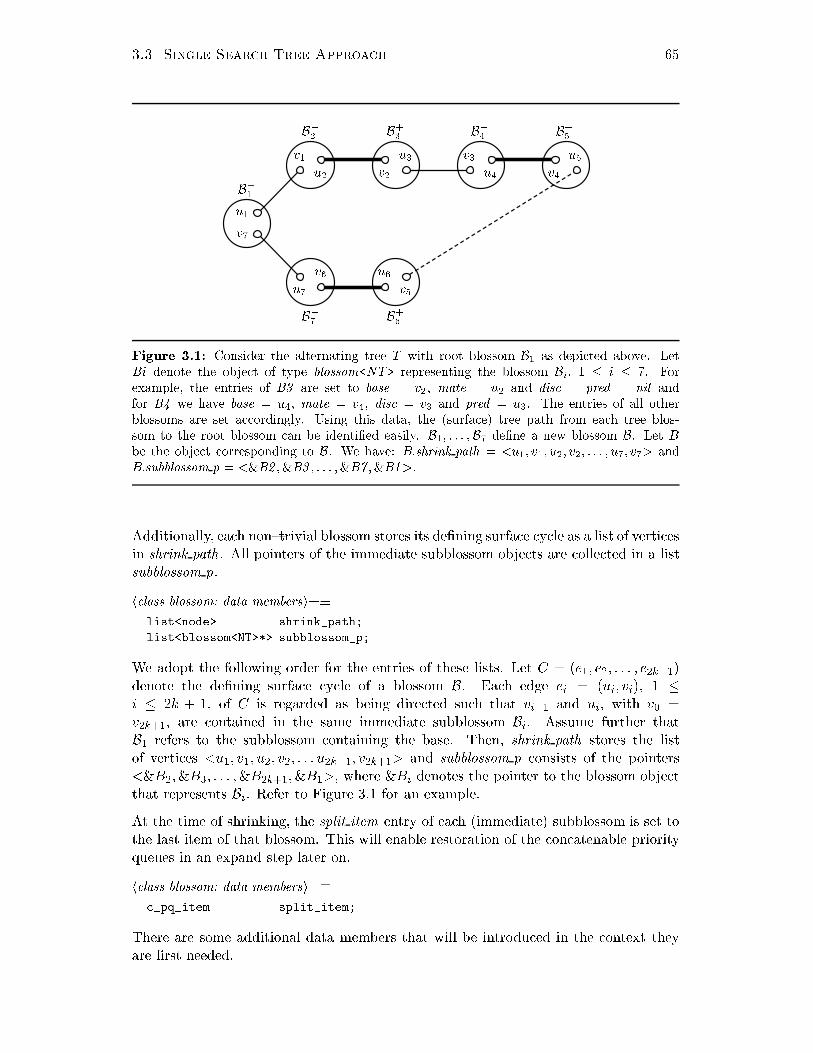
3.3 Single Sear h Tree Approa h 65v1 u2 v2u1B�2B+1 B+3u3 v3B�4u4 v4B+5

v7 u7 v6 u6 v5B�7 B+6u5

Figure 3.1: Consider the alternating tree T with root blossom B1 as depi ted above. LetBi denote the obje t of type blossom<NT> representing the blossom Bi, 1 � i � 7. Forexample, the entries of B3 are set to base = v2, mate = u2 and dis = pred = nil andfor B4 we have base = u4, mate = v4, dis = v3 and pred = u3. The entries of all otherblossoms are set a ordingly. Using this data, the (surfa e) tree path from ea h tree blos-som to the root blossom an be identi�ed easily. B1; : : : ;B7 de�ne a new blossom B. Let Bbe the obje t orresponding to B. We have: B:shrink path = <u1; v1; u2; v2; : : : ; u7; v7> andB:subblossom p = <&B2 ;&B3 ; : : : ;&B7 ;&B1>.Additionally, ea h non{trivial blossom stores its de�ning surfa e y le as a list of verti esin shrink path . All pointers of the immediate subblossom obje ts are olle ted in a listsubblossom p.h lass blossom: data membersi+�list<node> shrink_path;list<blossom<NT>*> subblossom_p;We adopt the following order for the entries of these lists. Let C = (e1; e2; : : : ; e2k+1)denote the de�ning surfa e y le of a blossom B. Ea h edge ei = (ui; vi), 1 �i � 2k + 1, of C is regarded as being dire ted su h that vi�1 and ui, with v0 =v2k+1, are ontained in the same immediate subblossom Bi. Assume further thatB1 refers to the subblossom ontaining the base. Then, shrink path stores the listof verti es <u1; v1; u2; v2; : : : u2k+1; v2k+1> and subblossom p onsists of the pointers<&B2;&B3; : : : ;&B2k+1;&B1>, where &Bi denotes the pointer to the blossom obje tthat represents Bi. Refer to Figure 3.1 for an example.At the time of shrinking, the split item entry of ea h (immediate) subblossom is set tothe last item of that blossom. This will enable restoration of the on atenable priorityqueues in an expand step later on.h lass blossom: data membersi+� _pq_item split_item;There are some additional data members that will be introdu ed in the ontext theyare �rst needed.

66 Chapter 3. Implementation and TestsMember Fun tions: We outline only some of the member fun tions; the remainingfun tions will be �lled in as needed. A fun tion that returns the (stored) redu ed ostof the best edge (of all best edges in ident to verti es) of a blossom is implemented asfollows.h lass blossom: member fun tionsi� onst NT min_prio() onst{ return (find_min() ? prio(find_min()) : INFINITY(NT)); }Here, INFINITY (NT ) simply returns the maximum value of type NT . The followingthree fun tions return the appropriate entries stored in the information part of an itemit (type pq item).h lass blossom: member fun tionsi+� onst NT pot_of ( _pq_item it) onst { return inf(it)->pot; } onst node node_of ( _pq_item it) onst { return inf(it)->my_node; } onst node best_adj( _pq_item it) onst { return inf(it)->best_adj; }We must also provide a fun tion to test whether or not a blossom is trivial: ea h blossom ontaining just one item is said to be trivial.h lass blossom: member fun tionsi+�bool trivial() onst { return size() == 1; }Friend Fun tions: Given the item it of a vertex, the following fun tion will returna pointer to the blossom obje t ontaining that vertex.h lass blossom: friend fun tions | de larationi�friend blossom<NT>* blossom_of<NT>( _pq_item it);The fun tion will also be used for testing whether or not two verti es are ontained inthe same blossom.When a new blossom obje t is reated, we all set owner (pt), where pt is the generi pointer of the new blossom obje t. Consequently, we an later ast the pointer returnedby get owner (it) to a pointer of type blossom<NT>�.h lass blossom: friend fun tions | de�nitioni�template< lass NT> blossom<NT>* blossom_of( _pq_item it) {return (it ? (blossom<NT>*)(get_owner(it)) : nil);}Constru tor: We are now in a position to de�ne the onstru tor of the lass blossom .As an optional argument, the base vertex b of the blossom to be reated an be given.h lass blossom: member fun tionsi+�blossom(node b = nil) : on at_pq<NT, vertex<NT>*>() {set_owner(leda_ ast(this));label = even;

3.3 Single Sear h Tree Approa h 67pot = offset = 0;base = b; mate = nil;dis = pred = nil;marker1 = marker2 = 0;item_in_T = item_in_O = nil;item_in_pq = nil;split_item = nil;}leda ast(this) simply asts the blossom pointer this to a generi pointer. The meaningof the missing data members marker1 , marker2 , item in T , item in O and item in pqwill be ome lear shortly.We also de�ne a friend fun tion that provides a more onvenient way of onstru tingand initializing a trivial blossom obje t. The fun tionh lass blossom: friend fun tions | de larationi+�friend _pq_item new_blossom<>(NT d, node b, blossom<NT>* &B); reates a new blossom obje t that onsists only of the vertex b having potential d. After-wards, B points to this new blossom obje t and the pq item of the item orrespondingto b is returned.h lass blossom: friend fun tions | de�nitioni+�template< lass NT> _pq_item new_blossom(NT d, node b, blossom<NT>* &B) {B = new blossom<NT>(b);vertex<NT> *v = new vertex<NT>(d, b);return B->init(INFINITY(NT), v);}Note that we do not use the data member pot of the blossom lass to store the potentialof b | in fa t, that data member is only used to maintain the potential of a non{trivial blossom. The priority of the item orresponding to b is set to INFINITY (NT )indi ating that urrently no best edge is available.3.3.2 AlgorithmLet us turn to the implementation of Algorithm 1.6.3 that realizes the ideas outlined inChapter 2. The algorithm maintains the lower bounds Æ1; : : : ; Æ4 by the following datastru tures.hlo al variablesi�NT delta1;NT delta2a;p_queue<NT, blossom<NT>*> delta2b;p_queue<NT, edge> delta3;p_queue<NT, blossom<NT>*> delta4;node resp_d1;edge resp_d2a;

68 Chapter 3. Implementation and Testsdelta1 keeps tra k of the minimum (stored) potential of an even tree vertex that hasbeen en ountered. delta1 is only used in the non{perfe t mat hing ase. The (a tual)value of delta2a represents the (a tual) redu ed ost of the best edge of all best edgesfrom an even non{tree vertex to an even tree vertex. The responsible vertex or edgeof delta1 and delta2a is stored in resp d1 and resp d2a , respe tively.6 An item hp; ptiin delta2b represents the best edge of an unlabeled blossom pointed to by pt . The(a tual) priority of p equals the (a tual) redu ed ost of this edge. Ea h edge e thatis a andidate for a shrink step has an item hp; ei in delta3 . The (a tual) priority of pequals one half of the (a tual) redu ed ost of edge e. delta4 ontains one item hp; ptifor ea h non{trivial tree blossom. pt is a pointer to the blossom obje t and the (a tual)priority of p equals one half of the (a tual) potential of that blossom.In Chapter 2 (Se tion 2.3 and Se tion 2.4) we have dis ussed the semanti s of ea h itemin any of those priority queues in more detail; we will not repeat that dis ussion here.A ounter Delta is used to a umulate the total sum of dual adjustments that havebeen performed up to the urrent stage of the algorithm.hlo al variablesi+�NT Delta = 0;We need a me hanism to identify the pq item in delta2b or delta4 orresponding to ablossom obje t. Therefore, we add the following data member to the blossom lass.h lass blossom: data membersi+�pq_item item_in_pq;Whenever a blossom sends an item to delta2b or delta4 , the orresponding pq item isstored in item in pq of that blossom.When a vertex be omes an even tree vertex, its in ident edges will be s anned; it mayhappen that several verti es be ome even tree verti es at on e. Therefore, all new eventree verti es are olle ted in a queue Q whi h is realized by a singly linked list of verti es(type node slist).hlo al variablesi+�node_slist Q(G);At the end of a phase the urrent alternating tree is destroyed and all priorities in ea h on atenable priority queue need to be reset to in�nity . We therefore a umulate in Tall pointers to surfa e blossoms that are part of the urrent alternating tree; and in Othe pointers of all unlabeled surfa e blossoms (outside of T ) that are adja ent to anyeven tree blossom.hlo al variablesi+�list<blossom<NT>*> T;list<blossom<NT>*> O;6In Chapter 2, we assumed that ea h even tree vertex has an item in a priority queue delta1 ; andthat ea h even non{tree surfa e blossom has an item in a priority queue delta2 . However, it is suÆ ientin fa t to keep tra k of the data as des ribed above: initiating the orresponding step for resp d1 orresp d2a will terminate the urrent phase.

3.3 Single Sear h Tree Approa h 69Sin e we must be able to identify a blossom's item (type list item) in T or O, ea hblossom obje t stores this list item in the data member item in T or item in O , respe -tively.h lass blossom: data membersi+�list_item item_in_T;list_item item_in_O;An array item of (type node array< pq item>) is used to identify the orrespondingitem (type pq item) for ea h vertex of G.hlo al variablesi+�node_array< _pq_item> item_of(G);Finally, we introdu e some variables that are used frequently. M is a list of edges andwill be used to represent the resulting mat hing. The maximum value of number typeNT is stored in INFTY .hlo al variablesi+�edge e;node resp, opst, ur, adj, u, v, r;blossom<NT> *RESP, *OPST, *CUR, *ADJ, *R;list<edge> M; onst NT INFTY = INFINITY(NT);The overall stru ture of the algorithm omputing either a maximum{weight mat hingor a maximum{weight perfe t mat hing is as follows.hSST.t: algorithmi�template< lass NT>list<edge> MWM_SST( onst ugraph &G, onst edge_array<NT> &w,node_array<NT> &pot, array<two_tuple<NT, int> > &BT,node_array<int> &b, int heur = 1, bool perfe t = false) {hlo al variablesihinitializationiforall_nodes(r, G) {R = _BLOSSOM_OF(r);if (R->mate) ontinue;h lear priority queues and QiR->status_ hange(even, Delta, T, Q);bool terminate = false;while (!terminate) {hs an all edges of verti es in Qihdetermine lower bounds and2b, : : : , and4 iif (delta2a == Delta) {haugment step using best edge of delta2aiterminate = true;}else if (delta1 == Delta) {

70 Chapter 3. Implementation and Testshalternate step using best node of delta1 iterminate = true;}else if ( and2b == Delta) {hgrow step using best edge of delta2bi}else if ( and3 == Delta) {hshrink step using best edge of delta3 i}else if ( and4 == Delta) {hexpand step using best blossom of delta4 i}else {hdual adjustmenti}}}hextra t mat hing and he ker informationireturn M;}In a main loop, we iterate over all verti es r of G. When the blossom R of r isunmat hed, i.e. the mate of R equals nil , a phase is initiated. We de�ne the followingma ro in order to more elegantly retrieve the pointer to the blossom obje t ontaininga given vertex.hSST.t: data stru turesi+�#define _BLOSSOM_OF(this_node) \(this_node ? blossom_of<NT>(item_of[this_node℄) : nil)At the beginning of ea h phase, delta1 ; : : : ; delta4 are reset and the queue Q is madeempty.h lear priority queues and Qi�delta1 = delta2a = INFTY;delta2b. lear(); delta3. lear(); delta4. lear();Q. lear();R is made an even tree blossom alling the member fun tionvoid status hange(LABEL l, NT Delta, list<blossom<NT>*> &T, node slist &Q)the implementation of whi h will be given shortly. In the inner while loop, we �rsts an all edges in ident to verti es of Q in order to maintain delta1 ; : : : ; delta4 orre tly.Then, the minimum priorities of delta2b, delta3 and delta4 are determined and storedin and2b, and3 and and4 , respe tively.hdetermine lower bounds and2b, : : : , and4 i�NT and2b = (delta2b.empty() ? INFTY : delta2b.prio(delta2b.find_min()));NT and3 = (delta3.empty() ? INFTY : delta3.prio(delta3.find_min()));NT and4 = (delta4.empty() ? INFTY : delta4.prio(delta4.find_min()));

3.3 Single Sear h Tree Approa h 71Thereafter, it is he ked if any of those lower bounds equals zero.7 If so, the appropriatestep is initiated. Note that between two onse utive dual adjustments, di�erent stepsmay have to be exe uted. We adopt the onvention that all grow steps pre ede asingle shrink step, and, further, all shrink steps pre ede any expand step. This seemsreasonable to us, sin e extending the tree in grow steps is rather heap ompared to ashrink step. Moreover, an expand step turned out to be more ostly than a shrink step.Finally, when we an hoose between either an augment step or an alternate step, weprefer the augment step. An augment step will de rease the number of free verti es bytwo, whereas an alternate step produ es only a de rease by one. When neither of thesesteps an be exe uted, a dual adjustment is performed in order to progress.hdual adjustmenti�NT delta = leda_min(delta1,leda_min(delta2a,leda_min( and2b,leda_min( and3, and4))));if ((delta == INFTY) && perfe t) return M; // return empty mat hingDelta = delta; // orresponds to Delta += (delta - Delta)A phase terminates, when either the ase delta1 == Delta (this never happens in theperfe t mat hing ase) or delta2a == Delta has o urred; or delta an be hosen asINFTY and thus no perfe t mat hing exists (in the perfe t mat hing ase only). Inthe latter ase, we return the empty mat hing.Initialization: Depending on the value assigned to the argument heur , the algorithmuses a di�erent method to ompute an initial mat hing and the vertex potentials.hinitializationi�int free = G.number_of_nodes();node_array<node> mate(G, nil);swit h(heur) { ase 0: { hempty mat hingi break; } ase 1: { hgreedy mat hingi break; }default: { hjump start mat hingi break; }}All three methods use the node array pot to store the initial potential of ea h vertexand a node array mate to represent the mat hing. free denotes the number of freeverti es.When the initial mat hing leaves no vertex unmat hed it will be optimal and we animmediately return it.7Remember that the a tual priorities are omputed by subtra ting Delta from the stored priorities.Therefore, an a tual priority equals zero i� the stored priority equals Delta.

72 Chapter 3. Implementation and Testshinitializationi+�if (free == 0) {hprepare solutionireturn M;}Otherwise, for ea h vertex u of G a trivial blossom CUR with potential pot [u℄ is on-stru ted; the orresponding pq item is stored in item of [u℄. When mate[u℄ is di�erentfrom nil , the data member mate of CUR is set to the vertex mate[u℄ and CUR getsunlabeled.hinitializationi+�forall_nodes(u, G) {item_of[u℄ = new_blossom<NT>(pot[u℄, u, CUR);if (mate[u℄) {CUR->mate = mate[u℄;CUR->label = unlabeled;}}Starting with an empty mat hing, the potentials are set as outlined in Se tion 1.6.3.hempty mat hingi�forall_nodes(u, G) {if (outdeg(u) == 0) { pot[u℄ = 0; ontinue; }NT max = -INFTY;forall_adj_edges(e, u) max = leda_max(w[e℄, max);pot[u℄ = max/2;}For ea h vertex u we determine the value max whi h is maximum along all edge weightsof in ident edges. The potential of u is set to max=2; pot [u℄ is set to zero, when noin ident edge exists.The onstru tion of a greedy mat hing or a jump start mat hing will be the subje t ofSe tion 3.5. For now, it shall be suÆ ient to regardhgreedy mat hingi�free = greedy_mat hing(G, w, pot, mate, perfe t);andhjump start mat hingi�free = jump_start(G, w, pot, mate, perfe t);as bla k{boxes that return the appropriate data in pot , mate and free.In ase all verti es are mat hed after the initial mat hing has been omputed, M anbe onstru ted as shown below.

3.3 Single Sear h Tree Approa h 73hprepare solutioni�forall_edges(e, G) {u = sour e(e);v = target(e);if (mate[u℄ && (mate[u℄ == v) &&mate[v℄ && (mate[v℄ == u))M.push(e);}For ea h edge e, it is he ked whether the endpoints are the mates of ea h other, ornot; if so, e is a mat hing edge and added to M . Observe that the information neededto he k optimality is set orre tly: pot ontains the potential of ea h vertex; BT isempty and all entries in the node array b are set to �1, indi ating that ea h vertex isa surfa e blossom.Performing a Status Change: We next outline the member fun tion of lassblossom that realizes a status hange.h lass blossom: member fun tionsi+�void status_ hange(LABEL l, NT Delta, list<blossom<NT>*> &T, node_slist &Q) {if (l == unlabeled) {hmake unlabeled non{tree blossomi}else if (l == odd) {hmake odd tree blossomi}else if (l == even) {hmake even tree blossomi}label = l;}The new status of the blossom obje t is determined by the given label l. The fun tionneeds to adjust the o�set of the blossom by some Delta as developed in Se tion 2.1.Moreover, T and Q must be maintained orre tly.When a blossom gets unlabeled, its o�set is adjusted depending on its urrent labellabel and the list item item in T of that blossom is deleted from T . Note that only treeblossoms an get unlabeled.hmake unlabeled non{tree blossomi�assert((label != l) && item_in_T);offset += (label == odd ? Delta : -Delta);T.del(item_in_T);item_in_T = nil;We only allow non{tree blossoms to be ome odd tree blossoms.8 The o�set is de reasedby Delta and its pointer is added to T .8Why a blossom an hange its status from being an even labeled non{tree blossom to an odd labeledtree blossom will be ome apparent when the realization of an augment step is inspe ted more losely.

74 Chapter 3. Implementation and Testshmake odd tree blossomi�assert((label != l) && !item_in_T);offset -= Delta;item_in_T = T.append(this);Consider the ase where a blossom be omes an even tree blossom. When its label isodd , we only need to update the o�set . Otherwise, the blossom is a non{tree blossom.The o�set gets adjusted and its pointer is added to T .hmake even tree blossomi�assert((label != l) || !item_in_T);if (label == odd) offset += 2*Delta;else { // non-tree blossomoffset += Delta;item_in_T = T.append(this);}happend all verti es to QiThere is something more to do here: all verti es ontained in the blossom obje t mustbe appended to Q. Therefore, we iterate over all items it of the blossom and appendthe vertex of this item (i.e. node of (it)) to Q. Some preparatory work is done as well.happend all verti es to Qi� _pq_item it;forall_items(it, *this) {inf(it)->pot += offset;Q.append(node_of(it));}if (!trivial()) pot -= 2*offset;offset = 0;The potential of ea h vertex ontained in the blossom and the potential of the blossomitself (if non{trivial) is adjusted su h that these a tual potentials are omputed orre tlywith respe t to the new o�set o�set = 0. Sin e every vertex of the blossom has to beinspe ted anyway, it is reasonable to use the provident strategy (see Se tion 2.1.3) atthis point.S anning New Even Verti es: For all verti es that have been added to Q, i.e. theverti es that have re ently be ome even tree verti es, the in ident edges have to bes anned in order to keep the data in the global priority queues delta1 to delta4 as wellas the redu ed ost of edges asso iated with verti es orre tly.hs an all edges of verti es in Qi�NT ur_pot, adj_pot, a tual_p, stored_p;while (!Q.empty()) { ur = Q.pop();CUR = _BLOSSOM_OF( ur); ur_pot = ompute_potential(CUR, Delta, item_of[ ur℄);if (!perfe t) {htry to improve delta1 i

3.3 Single Sear h Tree Approa h 75}forall_adj_edges(e, ur) {adj = opposite( ur, e);ADJ = _BLOSSOM_OF(adj);hdis ard dead and tree edgesiadj_pot = ompute_potential(ADJ, Delta, item_of[adj℄);a tual_p = ur_pot + adj_pot - w[e℄;hprune edgesiif ((ADJ->label == even) && !ADJ->item_in_T) {hnew delta2a edge en ounteredi}else if (ADJ->label == unlabeled) {hnew delta2b edge en ounteredi}else if (ADJ->label == even) // ADJ is even tree blossomdelta3.insert(a tual_p/2 + Delta, e);else if (ADJ->label == odd) {stored_p = a tual_p - ADJ->offset;ADJ->improve_ onne tion(item_of[adj℄, stored_p, ur);}}}For ea h vertex ur of Q we ompute its a tual potential ur pot alling the templatefun tion ompute potential , whi h is essentially a realization of the Formulae (2.1) and(2.2) of Se tion 2.1. The fun tion an also be asked to ompute the a tual potential ofa blossom CUR by setting it to nil .hSST.t: helpersi�template< lass NT>NT ompute_potential(blossom<NT> *CUR, NT Delta, _pq_item it = nil) {int a = (it == nil ? -2 : 1);int sigma = 0;if (CUR->item_in_T) sigma = (CUR->label == even ? -1 : 1);NT stored = (it == nil ? CUR->pot : CUR->pot_of(it));return stored + a * CUR->offset + a * sigma * Delta;}When ur pot is the new minimum potential of all even tree verti es, delta1 and resp d1are set a ordingly (only in non{perfe t mat hing ase).htry to improve delta1 i�if ( ur_pot < delta1 - Delta) {delta1 = ur_pot + Delta;resp_d1 = ur;// if (delta1 == Delta) break;}When the new (a tual) value of delta1 equals zero, i.e. delta1 ==Delta , we ould alsoimmediately break the s an step. The alternate step for resp d1 would de rease thenumber of free verti es by one and terminate the phase. However, we defer this step

76 Chapter 3. Implementation and Testsand omplete the s anning pro edure instead. The reason for doing so is that delta2amight also get de reased to zero and the orresponding augment step will then de reasethe number of free verti es by two.All edges e in ident to ur are onsidered. The potential of ea h adja ent vertex adjis omputed so as to enable the omputation of the a tual redu ed ost a tual p of e.However, dead edges or tree edges are dis arded:hdis ard dead and tree edgesi�// do not onsider edges within a blossomif (CUR == ADJ) ontinue;// do not onsider tree edgesif ((ADJ->label == odd) &&((ADJ->base == adj && ADJ->mate == ur) ||(ADJ->dis == adj && ADJ->pred == ur))) ontinue;Moreover, we use a pruning strategy. Sin e a phase terminates when the stored priorityof delta1 (in non{perfe t ase only) or delta2a equals Delta, we an dis ard all edges ewhose stored priority ex eeds the minimum value of delta1 and delta2a . We will say eis hopeless. Note, in the ase where e is a andidate edge for a shrink step, its storedpriority in delta3 will equal a tual p=2 +Delta.9hprune edgesi�#if !defined(_NO_PRUNING)if ((ADJ->label == even) && ADJ->item_in_T) {if (a tual_p/2 + Delta > leda_min(delta1, delta2a)) ontinue;}else if (a tual_p + Delta > leda_min(delta1, delta2a)) ontinue;#endifDepending on the status of ADJ , four ases are distinguished. First, when ADJ is aneven non{tree blossom, a new delta2a edge has been en ountered.hnew delta2a edge en ounteredi�if (a tual_p < delta2a - Delta) {delta2a = a tual_p + Delta;resp_d2a = e;if (delta2a == Delta) break;}We he k whether e is the new best edge of delta2a ; if ne essary, we update the value ofdelta2a and set resp d2a , a ordingly. In ase where the new (a tual) value of delta2aequals zero, we break the s an step immediately.Se ond, when ADJ is an unlabeled non{tree blossom, a new delta2b edge has beenen ountered.9The user an swit h o� the pruning strategy by de�ning the token NO PRUNING (#defineNO PRUNING) before the �le MWM.t is in luded.

3.3 Single Sear h Tree Approa h 77hnew delta2b edge en ounteredi�stored_p = a tual_p - ADJ->offset + Delta;if (ADJ->improve_ onne tion(item_of[adj℄, stored_p, ur))if (ADJ->item_in_pq)delta2b.de rease_p(ADJ->item_in_pq, a tual_p + Delta);else {ADJ->item_in_pq = delta2b.insert(a tual_p + Delta, ADJ);ADJ->item_in_O = O.append(ADJ);}The stored redu ed ost stored p of e is omputed a ording to (2.5) (as des ribed inSe tion 2.1.2). We he k whether e is the new best edge of adj to an even labeled treevertex and, if so, update the data of the orresponding item by the following memberfun tion:h lass blossom: member fun tionsi+�bool improve_ onne tion( _pq_item it, NT x, node u) {if (!it) return false;NT old_min = min_prio();if (de rease_p(it, x)) inf(it)->best_adj = u;return old_min != min_prio();}When the new priority x is less than the one urrently stored with it , i.e. fun tionde rease p returns true, the best adj entry is set to u. The fun tion returns true i� theminimum priority of the blossom obje t has hanged.In ase e is the new best edge of ADJ , we either de rease the orresponding item indelta2b (if there exists any), or insert an appropriate one. In the latter ase, ADJ isadditionally inserted into O.The last two ases are easy. For an even tree blossom ADJ , an appropriate item issimply inserted into delta3 ; and for an odd tree blossom ADJ , we all the memberfun tion improve onne tion as des ribed above.Alternate Step: We ome to the alternate step whi h is initiated when the a tualvalue of the minimum item in delta1 equals zero. Remember that this will never happenin the perfe t mat hing ase.halternate step using best node of delta1 i�RESP = _BLOSSOM_OF(resp_d1);RESP->base = resp_d1;alternate_path(RESP, item_of);hdestroy alternating tree T iRESP->label = even;First, the surfa e blossom RESP of resp d1 is retrieved. The alive edges along theeven length path from RESP to the root blossom of the tree are alternately unmat hedand mat hed. RESP will be ome free. The base of RESP is set to resp d1 , sin e thatvertex has (a tual) potential zero and thus is allowed to stay unmat hed. The urrentalternating tree gets destroyed (as will be des ribed below). Thereafter, RESP will

78 Chapter 3. Implementation and Testsbe an unlabeled non{tree blossom. Remember, however, that free non{tree blossomsare supposed to be even. Therefore, RESP 's label is orre ted to even (we do not allstatus hange).Next, we des ribe the fun tion alternate path whi h alternates the alive edges along thetree path from RESP to the root blossom of the tree. More pre isely, ea h mat hingedge along this path will be ome non{mat hing and ea h non{mat hing edge be omesmat hing. Re all that mat hing edges are represented by means of the data membersbase and mate of lass blossom. The fun tion will be reused in the augment step below.hSST.t: helpersi+�template< lass NT>void alternate_path(blossom<NT>* RESP, node_array< _pq_item> &item_of) {if (!RESP) return;blossom<NT> *CUR = RESP;node pred = RESP->base, dis = nil, mate;while (CUR) {if (CUR->label == even) {mate = CUR->mate;CUR->mate = dis ;CUR->base = pred;CUR = _BLOSSOM_OF(mate);}else { // CUR->label == oddpred = CUR->pred;dis = CUR->dis ;CUR->mate = pred;CUR->base = dis ;CUR = _BLOSSOM_OF(pred);}}}Starting at CUR = RESP , we follow the tree path towards the root. We keep thefollowing invariants: pred and dis denote the prede essor and dis overy vertex, re-spe tively, of the odd blossom whi h has been onsidered most re ently; initially, predis set to the base of RESP and dis is set to nil . For an even labeled tree blossom CUR,we store the former mate in mate and set its data members mate and base to dis andpred , respe tively. After this, the blossom to be inspe ted next is retrieved by using theformer mate information stored in mate. When CUR is an odd tree blossom, pred anddis are set, and the mate and base data members of CUR are set a ordingly. Thenext blossom to onsider is the blossom of pred .Augment Step: When the a tual redu ed ost of resp d2a equals zero, the urrent(surfa e) mat hing is augmented. We need to determine the two surfa e blossoms RESPand OPST of the endpoints of edge e = resp d2a .

3.3 Single Sear h Tree Approa h 79hdetermine RESP and OPST of ei�resp = sour e(e);opst = target(e);RESP = _BLOSSOM_OF(resp);OPST = _BLOSSOM_OF(opst);if (!OPST->item_in_T) {leda_swap(resp, opst);leda_swap(RESP, OPST);}// invariant: OPST is tree blossomOPST denotes the blossom that is ontained in the alternating tree T . First, the evennon{tree blossom RESP is made an odd tree blossom (here we need to allow an evennon{tree blossom to be ome an odd tree blossom); its pred and dis entries are setappropriately.haugment step using best edge of delta2ai�e = resp_d2a;hdetermine RESP and OPST of eiRESP->status_ hange(odd, Delta, T, Q);RESP->pred = opst;RESP->dis = resp;alternate_path(RESP, item_of);hdestroy alternating tree T iThen, the edges along the tree path from RESP (traversing OPST ) towards the rootblossom of T are alternated alling alternate path . Finally, the alternating tree T getsdestroyed, as des ribed next.Destroy Tree: T stores all pointers to the surfa e blossoms ontained in the alter-nating tree. For ea h su h blossom CUR, we reset the priorities of all items to in�nityby alling the member fun tion reset (see Se tion 3.2), and perform a status hange:CUR gets unlabeled.hdestroy alternating tree T i�forall(CUR, T) {if (CUR->label == odd) {CUR->dis = CUR->pred = nil;CUR->item_in_pq = nil;}CUR->reset();CUR->status_ hange(unlabeled, Delta, T, Q);}T. lear();For an odd tree blossom CUR, the data members dis and pred as well as item in pqhave to be set to nil . Finally, T is made empty.Every unlabeled non{tree blossom that is adja ent to any even tree blossom ontainsat least one item whose priority di�ers from in�nity . All those items need to be reset(to in�nity).

80 Chapter 3. Implementation and Testshdestroy alternating tree T i+�forall(CUR, O) {CUR->reset();CUR->item_in_pq = nil;CUR->item_in_O = nil;}O. lear();The pointers of all unlabeled surfa e blossoms adja ent to any even tree blossom havebeen olle ted in O. Therefore, we all the member fun tion reset for ea h surfa eblossom pointed to by an entry CUR of O; nil gets assigned to CUR's data membersitem in pq and item in O . Alternatively, one ould also delete ea h onne tion from avertex ontained in CUR to an even tree vertex separately. However, it turned out that alling reset on e for ea h su h surfa e blossom is more eÆ ient. O is afterwards madeempty.Grow Step: The implementation of a grow step is as follows. First, we retrieve theunlabeled non{tree blossom RESP having a tual priority zero in delta2b.hgrow step using best edge of delta2bi�RESP = delta2b.inf(delta2b.find_min());delta2b.del_item(RESP->item_in_pq);RESP->item_in_pq = nil;The item of RESP in delta2b is deleted and item in pq is set to nil . The best edge ofRESP is stored with the minimum item. Using the member fun tions of lass blossom ,it is not diÆ ult to obtain resp and opst , the two endpoints of that edge.hgrow step using best edge of delta2bi+� _pq_item best = RESP->find_min();resp = RESP->node_of(best);opst = RESP->best_adj(best);The vertex resp is ontained in RESP , and opst denotes the even labeled vertex in thealternating tree. RESP be omes an odd tree vertex having opst and resp as prede essorand dis overy vertex, respe tively.hgrow step using best edge of delta2bi+�RESP->status_ hange(odd, Delta, T, Q);RESP->pred = opst;RESP->dis = resp;RESP is deleted from O and its data member item in O is set to nil , sin e it is nolonger an unlabeled non{tree blossom; noti e that RESP must have an item in O.hgrow step using best edge of delta2bi+�O.del_item(RESP->item_in_O);RESP->item_in_O = nil;We do not need to delete the onne tion stored with resp from RESP . This will bedone when the tree gets destroyed later on.

3.3 Single Sear h Tree Approa h 81Finally, when RESP is a non{trivial blossom, an item representing RESP and one halfof the value of its potential is inserted into delta4 .hgrow step using best edge of delta2bi+�if (!RESP->trivial())RESP->item_in_pq =delta4.insert( ompute_potential(RESP, Delta)/2 + Delta, RESP);The mate blossom MATE of RESP is also added to T . MATE be omes an even treeblossom.hgrow step using best edge of delta2bi+�node mate = RESP->mate;blossom<NT> *MATE = _BLOSSOM_OF(mate);MATE->status_ hange(even, Delta, T, Q);if (MATE->item_in_pq) {delta2b.del_item(MATE->item_in_pq);MATE->item_in_pq = nil;O.del_item(MATE->item_in_O);RESP->item_in_O = nil;}When MATE has an item in delta2b it must be removed; we also delete its item fromO.Shrink Step: A shrink step is more omplex. The minimum item in delta3 ontainingthe new tight edge e is deleted and the blossoms RESP and OPST ontaining theendpoints resp and opst of e are determined (as des ribed above).hshrink step using best edge of delta3 i�e = delta3.inf(delta3.find_min());delta3.del_min();hdetermine RESP and OPST of eiif (RESP == OPST) ontinue; // dead edge en ountered;In ase e is dead, i.e. RESP and OPST refer to the same blossom, we simply dis arde and ontinue with the main algorithm. Otherwise, we have to determine the lowest ommon an estor blossom LCA of RESP and OPST as well as the shrink path, i.e. thede�ning odd length surfa e y le, of the new blossom.hshrink step using best edge of delta3 i+�blossom<NT> *LCA;list<node> P1, P2;list<blossom<NT>*> sub1, sub2;hdetermine LCA and shrink path of RESP and OPST iThe ode hunk whi h implements this will be presented shortly. For the time being,assume sub1 and P1 orrespond to the lists subblossom p and shrink path of the newblossom as des ribed in Se tion 3.3.1. We onstru t a new surfa e blossom SUPERwhose base and mate equal those of LCA. Note that the priority queue of SUPER

82 Chapter 3. Implementation and Testsis empty. Its a tual potential is set to zero (the stored potential must hen e equal�2Delta); and P1 is assigned to its data member shrink path .hshrink step using best edge of delta3 i+�blossom<NT> *SUPER = new blossom<NT>(LCA->base);SUPER->pot = -2*Delta;SUPER->mate = LCA->mate;SUPER->shrink_path = P1;Subsequently, the priority queues of all subblossoms CUR of SUPER are on atenatedone after another, alling the member fun tion append subblossom dis ussed below.When CUR is an odd tree blossom and has sent an item to delta4 , this item is deleted.Finally, SUPER is added to the list of T .hshrink step using best edge of delta3 i+�forall(CUR, sub1) {if (CUR->item_in_pq) {delta4.del_item(CUR->item_in_pq);CUR->item_in_pq = nil;}SUPER->append_subblossom(CUR, Delta, T, Q);}SUPER->item_in_T = T.append(SUPER);We next need to �ll in details of the member fun tion append subblossom whi h helpsto on atenate the subblossoms.h lass blossom: member fun tionsi+�void append_subblossom(blossom<NT> *CUR, NT Delta,list<blossom<NT>*> &T, node_slist &Q) {if (CUR->label == odd)CUR->status_ hange(even, Delta, T, Q);if (!CUR->trivial())CUR->pot += -2*CUR->offset + 2*Delta;T.del(CUR->item_in_T);CUR->item_in_T = nil; on at(*CUR);CUR->split_item = last_item();subblossom_p.append(CUR);}Ea h odd subblossom is made even by alling the member fun tion status hange . In ase CUR is non{trivial, its potential gets frozen as explained (in Se tion 2.1.3). CURis deleted from T , sin e it is no longer a surfa e blossom. The priority queue of CURgets on atenated to that of the blossom obje t by alling the inherited fun tion on at .split item of CUR is set to the last item of the resulting priority queue (whi h is the lastitem of CUR), and CUR is appended to the subblossom p list of the urrent blossomobje t.

3.3 Single Sear h Tree Approa h 83Determination of the Lowest Common An estor: We will determine the lowest ommon an estor blossom of RESP and OPST by traversing the two tree paths towardsthe root in a lo k{step fashion.10We introdu e an additional ounter lo k , whi h is initially set to zero and will bein remented ea h time a lowest ommon an estor has to be determined; sin e lo kmight get in remented up to n2 times, type double has been hosen (in order to preventan over ow as might o ur for type int).hlo al variablesi+�double lo k = 0;Moreover, ea h blossom o upies two markers alled marker1 and marker2 .h lass blossom: data membersi+�double marker1, marker2;The way we determine the lowest ommon an estor is as follows. We traverse the treepaths from RESP and OPST towards the root. For ea h even blossom CUR1 on the�rst path (starting with RESP), we set marker1 to lo k ; and for ea h even tree blossomCUR2 on the se ond path (starting with OPST ), we set marker2 to lo k . The lowest ommon an estor blossom is en ountered when either marker2 of CUR1 or marker1of CUR2 equals lo k .hdetermine LCA and shrink path of RESP and OPST i�blossom<NT> *CUR1 = RESP, *CUR2 = OPST;CUR1->marker1 = CUR2->marker2 = ++lo k;P1.push(resp); P2.push(opst);while (CUR1->marker2 != lo k && CUR2->marker1 != lo k &&(CUR1->mate != nil || CUR2->mate != nil)) {if (CUR1->mate) {sub1.push(CUR1);P1.push(CUR1->base); P1.push(CUR1->mate);CUR1 = _BLOSSOM_OF(CUR1->mate);sub1.push(CUR1);P1.push(CUR1->dis ); P1.push(CUR1->pred);CUR1 = _BLOSSOM_OF(CUR1->pred);CUR1->marker1 = lo k;}if (CUR2->mate) {sub2.push(CUR2);P2.push(CUR2->base); P2.push(CUR2->mate);CUR2 = _BLOSSOM_OF(CUR2->mate);sub2.push(CUR2);P2.push(CUR2->dis ); P2.push(CUR2->pred);CUR2 = _BLOSSOM_OF(CUR2->pred);10A trivial method to determine the lowest ommon an estor of RESP and OPST is as follows.Starting at RESP we tra e the tree path up to the root, marking ea h traversed blossom. After this,following the tree path from OPST , the �rst marked blossom we meet will be the lowest ommonan estor. However, that method uses time O(n) per determination and thus would not omply withour worst{ ase bound of O(m log n) per phase.

84 Chapter 3. Implementation and TestsCUR2->marker2 = lo k;}}sub1.push(CUR1); sub2.push(CUR2);While we are tra ing the paths towards the lowest ommon an estor, we keep tra kof the subblossoms and edges traversed on either path. The lists sub1 and sub2 (typelist<blossom<NT>�>) ontain the pointers of all traversed surfa e blossoms from RESPand OPST to CUR1 and CUR2 in reversed order, respe tively. P1 and P2 (typelist<node>) onsist of all vertex pairs representing the (dire ted) alive path from RESPand OPST to CUR1 and CUR2 in reversed order, respe tively.Assume the while loop above is left, sin e marker1 of CUR2 equals lo k . CUR2 thendenotes the lowest ommon an estor blossom LCA. We orre t sub1 and P1 su h thatthe head of sub1 equals LCA and the �rst vertex pair of P1 orresponds to the �rst(dire ted) edge on the reversed tree path from RESP to LCA. The ase where CUR1equals the lowest ommon an estor blossom LCA is treated analogously.hdetermine LCA and shrink path of RESP and OPST i+�if (CUR2->marker1 == lo k) { // CUR2 is LCAwhile (sub1.head() != CUR2) {sub1.pop(); sub1.pop();P1.pop(); P1.pop();P1.pop(); P1.pop();}}else if (CUR1->marker2 == lo k) { // CUR1 is LCAwhile (sub2.head() != CUR1) {sub2.pop(); sub2.pop();P2.pop(); P2.pop();P2.pop(); P2.pop();}}// sub1.head() == sub2.head() == LCALCA = sub1.pop();sub2.reverse(); sub1. on (sub2);P2.reverse(); P1. on (P2);Finally, the on atenation of sub1 and sub2 (the �rst element of sub1 is popped andsub2 is reversed beforehand) yields the desired list sub1 orresponding to the listsubblossom p of the new blossom obje t as spe i�ed previously. Analogously, the on- atenation of P1 with the reversed path P2 orresponds to the shrink path of the newblossom.Expand Step: The responsible blossom RESP whi h is going to be expanded aneasily be obtained from delta4 .hexpand step using best blossom of delta4 i�RESP = delta4.inf(delta4.find_min());delta4.del_item(RESP->item_in_pq);

3.3 Single Sear h Tree Approa h 85Next, we need to re over the data for ea h (immediate) subblossom of RESP . Therefore,we de�ne a new member fun tion expand whi h restores the priority queue for ea hsubblossom of RESP and unfreezes the potential if ne essary. RESP is deleted from Tand the pointers of all subblossoms are added to T .hexpand step using best blossom of delta4 i+�RESP->expand(Delta);forall(CUR, RESP->subblossom_p)CUR->item_in_T = T.append(CUR);T.del(RESP->item_in_T);The details of the member fun tion expand are dis ussed next. Later on, we will alsouse that member fun tion to expand an even or unlabeled non{tree blossom. We iterateover all (immediate) subblossoms of the blossom obje t stored in the subblossom p list.For ea h subblossom CUR we split the urrent priority queue of the blossom obje t atCUR's split item into two. The �rst of whi h gets assigned to CUR and the remainingbe omes the new urrent priority queue of the blossom obje t (whi h will be split inthe next iteration). At the end, all subblossom priority queues are restored and thepriority queue of the blossom obje t is empty.h lass blossom: member fun tionsi+�void expand(NT Delta) {blossom<NT> *CUR;forall(CUR, subblossom_p) {split_at_item(CUR->split_item, *CUR, *this);CUR->offset = offset;CUR->label = label;if (!CUR->trivial() && label == odd)CUR->pot += 2*offset + 2*Delta;else if (!CUR->trivial()) {assert(!CUR->item_in_T);assert(CUR->label == even || CUR->label == unlabeled);CUR->pot += 2*offset;}}}Moreover, the o�set of ea h subblossom CUR is set to the o�set value of the blossomobje t. Re all that at the time of shrinking, we arranged that ea h subblossom is labeledeven. However, the a tual potential of ea h vertex, and the redu ed ost asso iated withit, is omputed orre tly with respe t to the status of the blossom obje t ontaining thatvertex. Therefore, ea h subblossom is labeled a ording to the blossom obje t ( allingstatus hange would be wrong). Finally, the potential of ea h non{trivial subblossomCUR gets unfrozen (by the formula given in Se tion 2.1.3).We an now determine the base blossom BASE and the dis overy blossom DISC ofRESP as follows.

86 Chapter 3. Implementation and Testshexpand step using best blossom of delta4 i+�blossom<NT> *BASE = _BLOSSOM_OF(RESP->base);blossom<NT> *DISC = _BLOSSOM_OF(RESP->dis );int dist = RESP->restore_mat hing(BASE, DISC);hextend alternating treeidelete RESP;The mat hing needs to be restored for the subblossoms. We do so by alling themember fun tion restore mat hing whi h will be the subje t of the next paragraph. Inthe ode hunk to extend the alternating tree, we will set up some additional data forthe subblossoms along the even length (alive) path from BASE to DISC , and, moreover,remove the remaining subblossoms from T . Finally, we an destroy the blossom obje tpointed to by RESP .Restoring the Mat hing: The member fun tion restore mat hing restores themat hing data for all subblossoms of the blossom obje t.h lass blossom: member fun tionsi+�int restore_mat hing(blossom<NT> *BASE, blossom<NT> *DISC) {h y li ally rotate subblossom p and shrink path listihalternately mat h/unmat h subblossoms along subblossom pireturn dist;}The idea is simple. We start at the base blossom BASE and alternately unmat h andmat h the edges along the odd length (alive) y le (represented by shrink path). Firstof all, we need to y li ally rotate the lists subblossom p and shrink path until the baseblossom BASE o urs at the end of subblossom p:h y li ally rotate subblossom p and shrink path listi�while (subblossom_p.tail() != BASE) {subblossom_p.append(subblossom_p.pop());shrink_path.append(shrink_path.pop());shrink_path.append(shrink_path.pop());}Note that the i{th vertex pair of shrink path orresponds to the in oming edge of thei{th subblossom on subblossom p. The mate and base entries of the BASE blossom areset to mate and base of the blossom obje t, respe tively.halternately mat h/unmat h subblossoms along subblossom pi�BASE->mate = mate;BASE->base = base;Then, the subblossoms along the subblossom p list are mat hed pairwise. In the pro ess,we keep tra k of the position dist of DISC in subblossom p; we start ounting with 1.

3.3 Single Sear h Tree Approa h 87halternately mat h/unmat h subblossoms along subblossom pi+�node b, m;int dist, pos = 1;list_item p_it = shrink_path.first();list_item sub_it = subblossom_p.first();blossom<NT> *CUR = subblossom_p.inf(sub_it), *ADJ;while (CUR != BASE) {if (CUR == DISC) dist = pos;sub_it = subblossom_p.su (sub_it); pos++;ADJ = subblossom_p.inf(sub_it);if (ADJ == DISC) dist = pos;p_it = shrink_path.su (p_it);p_it = shrink_path.su (p_it); b = shrink_path.inf(p_it);p_it = shrink_path.su (p_it); m = shrink_path.inf(p_it);CUR->base = b; CUR->mate = m;ADJ->base = m; ADJ->mate = b;sub_it = subblossom_p.su (sub_it); pos++;CUR = subblossom_p.inf(sub_it);p_it = shrink_path.su (p_it);}if (CUR == DISC) dist = pos;Extending the Alternating Tree: We need to set up some additional data, su h asthe pred and dis pointers et ., for the subblossoms of RESP lying on the even length(alive) path from BASE to DISC . Furthermore, all remaining subblossoms must leaveT . The way we a hieve the desired result is by another traversal of the blossom y le.We start at the base blossom BASE and follow the even length path to DISC , settingup the ne essary data for ea h tree blossom on this path. After this, all remainingsubblossoms on the blossom y le be ome unlabeled and leave T .Remember that dist stores the position of DISC in subblossom p and that BASE is thelast element in this list. Moreover, we know that the number of elements in subblossom pis odd. When dist is odd, the reversal of subblossom p ontains all subblossoms ofthe even length path from BASE to DISC followed by all subblossoms that leave T .Otherwise, when dist is even, we move BASE to the head of subblossom p. Again,subblossom p then onsists of the subblossoms of the even length path from BASE toDISC followed by the subblossoms leaving T .hextend alternating treei�if (dist % 2) {RESP->subblossom_p.reverse();RESP->shrink_path.reverse();}else RESP->subblossom_p.push(RESP->subblossom_p.Pop());We establish the following invariant for the vertex pairs along shrink path . The i{thvertex pair of shrink path orresponds to the outgoing edge of the i-th subblossom insubblossom p.

88 Chapter 3. Implementation and TestsNext, we turn to the set up of the data for the subblossoms staying in T . First, thedis overy and prede essor verti es of DISC are set a ordingly.hextend alternating treei+�DISC->dis = RESP->dis ;DISC->pred = RESP->pred;Next, the �rst two elements CUR and ADJ are popped from the subblossom p list;CUR orresponds to an odd blossom and ADJ to an even blossom. We set the predand dis entries for CUR; and in ase CUR is non{trivial, insert an item in delta4 .ADJ is made even. This pro ess is repeated until the urrent blossom CUR equalsDISC .hextend alternating treei+�CUR = RESP->subblossom_p.pop();while (CUR != DISC) {ADJ = RESP->subblossom_p.pop(); ur = RESP->shrink_path.pop();adj = RESP->shrink_path.pop();CUR->pred = adj; CUR->dis = ur;if (!CUR->trivial())CUR->item_in_pq =delta4.insert( ompute_potential(CUR, Delta)/2 + Delta, CUR);ADJ->status_ hange(even, Delta, T, Q);RESP->shrink_path.pop();RESP->shrink_path.pop();CUR = RESP->subblossom_p.pop();}// send item for DISC alsoif (!CUR->trivial())CUR->item_in_pq =delta4.insert( ompute_potential(CUR, Delta)/2 + Delta, CUR);Finally, ea h remaining blossom CUR in subblossom p gets unlabeled (and is therebyremoved from T ). When the priority queue of CUR is not empty, its best edge is sentto delta2b and CUR is inserted into O. Moreover, the pred and dis entries of CURneed to be set to nil .hextend alternating treei+�while (!RESP->subblossom_p.empty()) {CUR = RESP->subblossom_p.pop();CUR->status_ hange(unlabeled, Delta, T, Q);if (!CUR->empty()) {CUR->item_in_pq = delta2b.insert(CUR->min_prio() + CUR->offset, CUR);CUR->item_in_O = O.append(CUR);}CUR->pred = CUR->dis = nil;}This on ludes the dis ussion of all details on erned with an expand step.

3.3 Single Sear h Tree Approa h 89Extra ting Mat hing and Che ker Information: The algorithm terminates witha surfa e mat hing. We have to extra t the original mat hing M (type list<edge>) byexpanding all non{trivial blossoms (whi h are either labeled even or unlabeled).hextra t mat hing and he ker informationi�int k = 0;forall_nodes(v, G)unpa k_blossom(_BLOSSOM_OF(v), item_of, pot, b, BT, k, -1, Delta);if (k != 0) BT.resize(k);forall_edges(e, G)if (_BLOSSOM_OF(sour e(e))->mate == target(e)) M.push(e);We use a fun tion unpa k blossom whi h re ursively expands all subblossoms to a givenblossom; simultaneously, the information needed by the he ker will be onstru ted.A surfa e blossom is expanded ompletely, the �rst time when one of its verti es is onsidered. When all blossoms are expanded, we have to reset the index range ofBT to [0; : : : ; k � 1℄, where k will refer to the number of non{trivial surfa e blossoms.Finally, ea h mat hing edge is added to M .We turn to the des ription of the fun tion unpa k blossom :hSST.t: helpersi+�template< lass NT>void unpa k_blossom(blossom<NT> *RESP, onst node_array< _pq_item> &item_of,node_array<NT> &pot, node_array<int> &b,array<two_tuple<NT, int> > &BT,int &k, int parent, NT Delta) {if (RESP->trivial()) {hset up he ker data for trivial blossomi}else {hset up he ker data for non{trivial blossomiRESP->expand(Delta);blossom<NT> *BASE = _BLOSSOM_OF(RESP->base);blossom<NT> *DISC = nil;RESP->restore_mat hing(BASE, DISC);blossom<NT>* CUR;forall(CUR, RESP->subblossom_p)unpa k_blossom(CUR, item_of, pot, b, BT, k, idx, Delta);delete RESP;}}The fun tion reates the data pot , b and BT needed for the he ker. We dis ussedthe semanti s of these arrays in Se tion 3.1 and will not repeat the dis ussion here. kdenotes the index that is used to store the next non{trivial blossom data in BT . Weuse parent to pass the parent index of a non{trivial surfa e blossom to its (immediate)subblossoms.First, assume RESP is a trivial blossom ontaining only the vertex ur . When RESPhas already been expanded, i.e. b[ ur ℄ != �1, we immediately leave unpa k blossom .

90 Chapter 3. Implementation and TestsOtherwise, we simply set up its he ker data:hset up he ker data for trivial blossomi�node ur = RESP->node_of(RESP->first_item());if (b[ ur℄ != -1) return;pot[ ur℄ = ompute_potential(RESP, Delta, item_of[ ur℄);b[ ur℄ = parent;The a tual potential of the vertex ur is omputed and entered in pot [ ur ℄. b[ ur ℄ isset to the parent index parent (of the smallest non{trivial blossom ontaining ur ; or�1).When RESP is non{trivial, its he ker data is set up as follows.hset up he ker data for non{trivial blossomi�if (k > BT.high()) BT.resize(2*k+1);BT[k℄.first() = ompute_potential(RESP, Delta);BT[k℄.se ond() = parent;int idx = k++;We double the size of BT whenever k ex eeds the highest index of BT . The a tualpotential of RESP is omputed and stored in the �rst omponent of BT [k℄. RESP 'sparent index is stored in the se ond omponent. We keep the urrent value of k in idx(whi h will be used as the parent index for the re ursive alls) and in rement k.Subsequently, the subblossoms are expanded and the mat hing is restored for the (im-mediate) subblossoms of RESP . The fun tions needed to a hieve this were dis ussedfor the expand step (see above). Ea h immediate subblossom gets expanded re ursively,by alling unpa k blossom for it. The parent index for the re ursive alls is set to theindex value idx of RESP in BT .3.4 Multiple Sear h Tree Approa hThe eÆ ien y of a priority queue based implementation of Edmonds' blossom{shrinkingapproa h is substantially improved when several trees are grown simultaneously. Wenext sket h the basi ideas underlying our multiple sear h tree approa h. The imple-mentation details will be presented in the subsequent se tions.An alternating tree Ti is rooted at ea h free vertex ri. Ea h tree Ti is extended as in thesingle sear h tree approa h. That is, we perform alternate, grow, shrink and expandsteps as before. However, an augment step is performed di�erently: when a tight edgeuv, u+ 2 Ti and v+ 2 Tj with Ti 6= Tj exists, the urrent mat hing is augmented alongthe two tree paths (from u and v to their roots), and u and v get mat hed. A dualadjustment by Æ hanges the potentials of all verti es and surfa e blossoms as explainedin Se tion 1.6.3. As before, the value of Æ is determined by the lower bounds Æ1; : : : ; Æ4;Æ1 is only taken into a ount in the non{perfe t mat hing ase. But note that thede�nition of Æ3 needs to be re�ned now. The redu ed ost of an edge uv, with u+ 2 Ti,v+ 2 Tj and Ti 6= Tj , de reases by 2Æ for a dual adjustment. Therefore, the redu ed osts of those edges have to be taken into onsideration as well. More pre isely, we

3.4 Multiple Sear h Tree Approa h 91rede�ne Æ3 as follows:Æ3 = minuv2E f�uv=2 : u+ 2 Ti; v+ 2 Tjg;where Ti and Tj refer to any of the alternating trees (di�erent or equal).In the multiple sear h tree approa h, ea h vertex u keeps its best onne tion to analternating tree Ti. An edge uvi in ident to u is alled a best onne tion from u to Ti,when(1) vi is an even tree vertex in Ti, and(2) the (stored) redu ed ost �uvi is minimal along all other (stored) redu ed osts�uvj , with v+j 2 Ti, i.e. �uvi = minuvj2Ef�uvj : v+j 2 Tig:When several best onne tions from u to a �xed tree Ti exist, the best onne tion fromu to Ti will refer to any of those.For ea h vertex u we have a priority queue Pu whi h stores the best onne tions from uto all existing alternating trees. However, even tree verti es form an ex eption: whenu+ 2 Ti is an even tree vertex ontained in an alternating tree Ti, we do not keep thebest onne tion from u to its own tree Ti in Pu. When uvi is the best onne tion fromu to Ti, the orresponding item in Pu equals h�uvi ; vii, where �uvi denotes the (stored)redu ed ost of that edge.As before, ea h surfa e blossom B (trivial or non{trivial) is asso iated with a on- atenable priority queue PB. Ea h vertex u 2 B has a representative item in PB. Therepresentative item of a vertex u in PB orresponds to the minimum of all best onne -tions of u (with regard to the redu ed osts). Thus, the minimum item in PB representsthe best onne tion of B.In Se tion 2.1 we presented a strategy to handle the varying priorities for ea h of thesepriority queues.An alternating tree Ti olle ts all edges uv that are andidates for a shrink step,i.e. u+; v+ 2 Ti, in a priority queue PTi . The priority stored with ea h su h edgeuv orresponds to the (stored) redu ed ost of that edge. In the non{perfe t mat hing ase, Ti knows its even vertex u+i 2 Ti whose (stored) potential is minimum along alleven tree verti es in Ti.The way we will use the data asso iated with ea h surfa e blossom or alternating tree isas follows. Again, the lower bounds Æ1; : : : ; Æ4 that determine the value of Æ are realizedby means of the priority queues delta1 to delta4 .In the non{perfe t mat hing ase, ea h alternating tree Ti has a orresponding itemhyui ; uii in delta1 . u+i 2 Ti denotes the even vertex stored with Ti as introdu ed before;and yui equals the (stored) potential of ui.Ea h non{tree blossomBf?j+g sends its best onne tion to delta2 . An even labeled non{tree blossom will only o ur in the non{perfe t mat hing ase. The (a tual) priority ofea h item in delta2 equals the (a tual) redu ed ost of the represented edge.Æ3 is realized by two priority queues delta3a and delta3b . Generally speaking, delta3akeeps best onne tions that an be used for an augment step, and delta3b olle ts andidate edges for a shrink step. More pre isely, for ea h best onne tion of an even

92 Chapter 3. Implementation and Teststree blossom B+ 2 Ti, we have an appropriate item in delta3a .11 An alternating tree Tisends its best andidate edge uv from PTi to delta3b. In both priority queues, the a tualpriorities will orrespond to one half of the a tual redu ed ost of the orrespondingedges.Finally, in delta4 we olle t all odd tree blossoms. The a tual priority of ea h itemequals one half of the a tual potential of the orresponding blossom.The ideas outlined should suÆ e for the moment. All remaining details will be ome lear in the rest of this se tion, where we dis uss our implementation of a multiplesear h tree approa h. Many parti ulars have been presented for the single sear h treeapproa h in the pre eding se tion. We will therefore fo us on the ensuing modi� ationsand extensions.3.4.1 Data Stru turesWe ome to the data stru tures of our implementation.hMST.t: data stru turesi�template< lass NT> lass blossom;template< lass NT> lass vertex;template< lass NT> lass tree;h lass blossomih lass vertex ih lass treeiAs before, blossoms are represented by an obje t of lass blossom . All data membersand most of the member fun tions that have been introdu ed for that lass in thepre eding se tion will be reused.De�nition of the Additional Class vertex :We de�ne a lass vertex whi h keeps all data asso iated with a vertex. Its overallstru ture is given below.h lass vertex i�template< lass NT> lass vertex : publi virtual p_queue<NT, node> {publi :NT pot;node my_node;h_array<node, pq_item> ITEM_OF;h lass vertex: member fun tionsiLEDA_MEMORY(vertex<NT>);};11Here, we need to have ea h even tree vertex keep tra k of its best onne tions to other, i.e. di�erent,alternating trees.

3.4 Multiple Sear h Tree Approa h 93Class vertex inherits all properties of a priority queue (type p queue<NT ; node>). Thepriorities are of type NT and the information part refers to a vertex. Ea h best on-ne tion uvi of a vertex u to an alternating tree Ti is represented by an item h�uvi ; viiin the priority queue. As before, pot is set to the (stored) potential u and my nodedenotes the vertex u itself. We will need to identify the item orresponding to u'sbest onne tion to a given tree Ti. Therefore, we use a hashing array ITEM OF (typeh array<node ; pq item>) whi h maps the root vertex ri of a tree Ti to the appropriateitem (type pq item). h array is a dynami data type provided by LEDA. It is imple-mented by hashing with haining. All a ess operations take expe ted time O(1). Theoperations of this data type that are used will be explained brie y at the time they are�rst needed.Constru tor: The onstru tor of lass vertex is trivial. It simply reates a new vertexobje t for a vertex u having potential d.h lass vertex: member fun tionsi�vertex(NT d, node u) : p_queue<NT, node>() { pot = d; my_node = u; }The obje t is initialized with the empty priority queue, and ITEM OF is unde�ned forall verti es.Member Fun tions: We ome to some standard a ess fun tions. min prio returnsthe priority of the minimum item; and min inf the information part.h lass vertex: member fun tionsi+�NT min_prio() onst{ return (find_min() ? prio(find_min()) : INFINITY(NT)); }node min_inf() onst{ return (find_min() ? inf(find_min()) : nil); }As before, INFINITY (NT ) or nil is returned, respe tively, when the priority queue isempty.We also need to rede�ne the member fun tion best adj of lass blossom:h lass blossom: member fun tionsi+� onst node best_adj( _pq_item it) onst { return inf(it)->min_inf(); }This fun tion returns the vertex stored with the minimum item in the priority queueof a vertex obje t (inf (it)).The following member fun tion tries to improve the best onne tion of a vertex obje tto a tree, say T , rooted at r.h lass vertex: member fun tionsi+�bool de rease_p(node u, NT x, node r) {NT old_min = min_prio();if (!ITEM_OF.defined(r))

94 Chapter 3. Implementation and TestsITEM_OF[r℄ = insert(x, u);else {pq_item it = ITEM_OF[r℄;if (prio(it) > x) {p_queue<NT, node>::de rease_p(it, x);p_queue<NT, node>:: hange_inf(it, u);}}return old_min != min_prio();}u denotes the even tree vertex in T , and x will orrespond to the (stored) redu ed ostof the edge from my node to u. First, we he k whether the vertex obje t stores an itemrepresenting a best onne tion to T . We do so by means of a de�ned operation providedby the data type h array . de�ned(r) returns true, i� an item has been set for r. In the ase where r is not de�ned for ITEM OF , we insert a new item hx; ui representing thebest onne tion to T . ITEM OF [r℄ is set to the orresponding pq item (and hen eforthde�ned for r). Otherwise, we an retrieve the item it of the urrent best onne tion toT by an a ess operation ITEM OF [r℄. When x is smaller than the priority urrentlystored with it , the priority of it is de reased to x and the information is hanged to u.The fun tion returns true, i� the minimum priority of the vertex obje t has hanged.We will need a member fun tion to delete the best onne tion of a vertex obje t to atree rooted at r.h lass vertex: member fun tionsi+�bool del(node r) {if (!ITEM_OF.defined(r)) return false;NT old_min = min_prio();del_item(ITEM_OF[r℄);ITEM_OF.undefine(r);return old_min != min_prio();}Given the root vertex r, we an look up its item using the a ess operation ITEM OF [r℄;when ITEM OF is not de�ned for r nothing has to be done. This item is deleted fromthe priority queue and ITEM OF be omes unde�ned for r by alling unde�ne(r). If theminimum priority has hanged due to the deletion, the fun tion returns true; otherwisefalse.De�nition of the Additional Class tree:We de�ne a new lass tree to maintain the ne essary data for the alternating trees.h lass treei�h lass tree: friend fun tions | de�nitionitemplate< lass NT> lass tree {h lass tree: friend fun tions | de larationipubli :node root;

3.4 Multiple Sear h Tree Approa h 95node d1_node;list<blossom<NT>*> my_blossoms;p_queue<NT, edge> d3b_edges;pq_item item_in_d3b;h lass tree: member fun tionsiLEDA_MEMORY(tree<NT>);};An obje t T of lass tree (type tree<NT>) stores its root vertex in root . The pointers ofall surfa e blossoms ontained in T are olle ted in a list my blossoms . d1 node denotesan even vertex of T having minimum potential (along all even verti es of T ); this entrywill be used in the non{perfe t mat hing ase only. Additionally, ea h alternating treeT has its own priority queue d3b edges . An item hp; ei in d3b edges represents an edge ehaving (stored) redu ed ost p; moreover, e is a andidate for a shrink step, i.e. e = uvwith u+; v+ 2 T . The minimum item of d3b edges is sent as a representative to a globalpriority queue delta3b. item in d3b enables the identi� ation of this item in delta3b .p qWe brie y explain why we de ided to keep a separate priority queue for ea h alternating tree.One ould, alternatively, simply insert all these edges in the global priority queue delta3b. Butwhen an alternating tree T is destroyed after an augment step, we would need a me hanism toidentify all andidate edges of T in delta3b . Ea h su h edge would have to be deleted separatelyfrom delta3b onsuming time O(logm); or O(m logm) in total.In our strategy, however, we simply delete the representative of T (a essible by item in d3b)and make the priority queue d3b edges empty. This will take total time O(logm+m).x yEa h blossom stores a pointer to its alternating tree. That is, we add the followingdata member to the blossom lass:h lass blossom: data membersi+�tree<NT> *my_tree;When a new blossom obje t is onstru ted, my tree is set to nil . Furthermore, an a essoperation tree root is de�ned to return the root vertex of the alternating tree ontainingthe blossom.h lass blossom: member fun tionsi+� onst node tree_root() onst { return (my_tree ? my_tree->root : nil); }Constru tor: The onstru tion of a tree obje t is trivial. d1 node and item in d3bare set to nil . A root vertex r for the tree obje t to be reated an be given as anoptional argument.h lass tree: member fun tionsi�tree(node r = nil) { root = r; d1_node = nil; item_in_d3b = nil; }Initially, my blossoms is empty and d3b edges ontains no items.Member Fun tions: At this, we present only some basi member fun tions. Theremaining ones will be introdu ed when required.

96 Chapter 3. Implementation and TestsA blossom obje t (pointed to by) B is added to a tree as follows:h lass tree: member fun tionsi+�void add(blossom<NT> *B){ B->item_in_T = my_blossoms.append(B); B->my_tree = this; }B is appended to the list my blossom of the alternating tree. The item (type list item)of B in my blossoms is stored in the data member item in T of B; and my tree of B isset to the urrent tree obje t.Conversely, the removal of a blossom B from an alternating tree is realized by remove :h lass tree: member fun tionsi+�void remove(blossom<NT> *B){ my_blossoms.del(B->item_in_T); B->item_in_T = nil; B->my_tree = nil; }The operations needed to retrieve the priority or information part of the minimum itemin d3b edges are given below.h lass tree: member fun tionsi+� onst NT min_prio() onst {return (d3b_edges.find_min() ? \d3b_edges.prio(d3b_edges.find_min()) : INFINITY(NT)); } onst edge min_inf() onst{ return (d3b_edges.find_min() ? \d3b_edges.inf(d3b_edges.find_min()) : nil); }We de�ne an operation ins : it inserts an item hx; ei for an edge e having (stored)redu ed ost x into the priority queue d3b edges .h lass tree: member fun tionsi+�bool ins(NT x, edge e) {pq_item old_min = d3b_edges.find_min();d3b_edges.insert(x, e);return (old_min != d3b_edges.find_min());}The fun tion returns true, i� the minimum item in d3b edges has hanged.Friend Fun tions: We de lare a fun tion new tree that allows us to reate a newtree obje t more omfortably.h lass tree: friend fun tions | de larationi�friend tree<NT>* new_tree<>(node r, blossom<NT>* &B);It onstru ts a new tree obje t that represents an alternating tree rooted at r. B isthe only blossom ontained in this tree. The fun tion returns a pointer to the new treeobje t.

3.4 Multiple Sear h Tree Approa h 97h lass tree: friend fun tions | de�nitioni�template< lass NT> tree<NT>* new_tree(node r, blossom<NT>* &B) {tree<NT>* T = new tree<NT>(r);B->item_in_T = T->my_blossoms.append(B);return T;}3.4.2 AlgorithmThe data stru tures introdu ed above will suÆ e for our multiple sear h tree algorithm.We now pro eed to present the implementation details of the algorithm. Altogether,�ve priority queues will be needed:hlo al variablesi+�node_pq<NT> delta1(G);delta1 is a spe ialized priority queue of type node pq<NT>. A node pq is realized moreeÆ iently than a priority queue of type p queue<NT ; node>. However, it an only beused with the restri tion that ea h vertex o urs in at most one node pq . The data typesuits our purposes perfe tly. For ea h tree we set the priority of its d1 node in delta1to the (stored) potential of the vertex. Note that delta1 will only be used, however, inthe non{perfe t ase.hlo al variablesi+�p_queue<NT, blossom<NT>*> delta2;delta2 ontains an item hp; pti for ea h non{tree blossom. The a tual priority of pequals the a tual redu ed ost of the best onne tion of the blossom pointed to by pt .In the perfe t mat hing ase, ea h su h non{tree blossom will be unlabeled; however,in the non{perfe t mat hing ase also even labeled non{tree blossoms will o ur.hlo al variablesi+�p_queue<NT, blossom<NT>*> delta3a;p_queue<NT, tree<NT>*> delta3b;In delta3a , ea h item hp; pti refers to an even tree blossom (pointed to by pt). Thea tual priority of p equals one half of the a tual redu ed ost of the best onne tion ofthis blossom.Ea h alternating tree T sends an item hp; pti to delta3b . pt is a pointer to T . The a tualpriority of p orresponds to one half of the a tual redu ed ost of the best andidateedge for a shrink step in T (stored in d3b edges).hlo al variablesi+�p_queue<NT, blossom<NT>*> delta4;An item hp; pti in delta4 represents an odd tree blossom (pointed to by pt) havinga tual potential equal to one half of the a tual priority of p.Many lo al variables, as introdu ed for the single sear h tree algorithm, are needed hereas well. For instan e, the node array item of , the singly linked list of nodes Q (type

98 Chapter 3. Implementation and Testsnode slist), the global ounter Delta, the list of mat hing edgesM (type list<edge>), et .We will not dis uss their meaning again, but refer to the des ription in the pre edingse tion.The overall stru ture of the algorithm hanges slightly.hMST.t: algorithmi�template< lass NT>list<edge> MWM_MST( onst ugraph &G, onst edge_array<NT> &w,node_array<NT> &pot, array<two_tuple<NT, int> > &BT,node_array<int> &b, int heur = 1, bool perfe t = false) {hlo al variablesiint free = G.number_of_nodes();hinitializationiwhile (free) {hs an all edges of verti es in Qihdetermine lower bounds and1, : : : , and4 iif ( and3a == Delta) {haugment step using best onne tion of blossom in delta3aifree -= 2;}else if ( and1 == Delta) {halternate step using best node of delta1 ifree -= 1;}else if ( and2 == Delta) {hgrow or augment step using best onne tion of blossom in delta2 i}else if ( and3b == Delta) {hshrink step using best edge in delta3bi}else if ( and4 == Delta) {hexpand step using best blossom of delta4 i}else {hdual adjustmenti}}hextra t mat hing and he ker informationireturn M;}The ounter free has to be interpreted as follows. In the perfe t mat hing ase, freesimply refers to the number of free verti es. But in the non{perfe t mat hing ase,free denotes the number of free verti es having (a tual) potential larger than zero,i.e. the number of verti es that violate ( s)(2) (see Se tion 1.6.1). An alternate stepwill de rease free by 1, whereas an augment step de reases free by 2.We determine the minimum value and1 , and2 , and3a , and3b and and4 of ea hpriority queue delta1 , delta2 , delta3a , delta3b and delta4 , respe tively:

3.4 Multiple Sear h Tree Approa h 99hdetermine lower bounds and1, : : : , and4 i�NT and1 = (delta1.empty() ? INFTY : delta1.prio(delta1.find_min()));NT and2 = (delta2.empty() ? INFTY : delta2.prio(delta2.find_min()));NT and3a = (delta3a.empty() ? INFTY : delta3a.prio(delta3a.find_min()));NT and3b = (delta3b.empty() ? INFTY : delta3b.prio(delta3b.find_min()));NT and4 = (delta4.empty() ? INFTY : delta4.prio(delta4.find_min()));When any of these values equals Delta (and hen e the a tual priority equals zero),the appropriate step is initiated. Regarding the spe i� order of these steps, the samearguments apply as were given for the single sear h tree approa h. The realization ofea h step will be dis ussed below.We perform a dual adjustment as follows. The ode is similar to the one dis ussed forthe single sear h tree algorithm.hdual adjustmenti�NT delta = leda_min( and1,leda_min( and2,leda_min( and3a,leda_min( and3b, and4))));if ((delta == INFTY) && perfe t) return M; // return empty mat hingDelta = delta; // orresponds to Delta += (delta - Delta)When the value of free drops to zero, the algorithm terminates. We extra t the mat hingand he ker information in exa tly the same way as has been des ribed for the singlesear h tree approa h; therefore, the ode realizing this will not be repeated here.Initialization: The initialization di�ers only slightly. As before, depending on thevalue of heur we onstru t either an empty mat hing, a greedy mat hing or a jumpstart mat hing. Remember that the node array smate and pot represent the onstru tedmat hing and the vertex potentials. What di�ers is the way we set up the data for ea hblossom:hinitializationi+�forall_nodes(u, G) {item_of[u℄ = new_blossom<NT>(pot[u℄, u, CUR);if (mate[u℄) {CUR->mate = mate[u℄;CUR->label = unlabeled;}else {CUR->my_tree = new_tree<NT>(u, CUR);Q.append(u);}}For ea h vertex u of G we onstru t a trivial blossom CUR onsisting of u only. Thepotential of u is set to pot [u℄. When u is mat hed, its mate is stored in the data membermate of CUR, and CUR gets unlabeled. Otherwise, we onstru t a new alternatingtree whi h is rooted at u. CUR is the only blossom of this tree obje t; we let my tree

100 Chapter 3. Implementation and Testsof CUR point to the obje t. u is added to Q su h that the priority queue data for ea hadja ent vertex of u will be set up orre tly when all edges in ident to any vertex in Qare s anned for the �rst time.Performing a Status Change: We next revise the member fun tion of lass blossomthat performs a status hange. The overall stru ture remains the same.h lass blossom: member fun tionsi+�void status_ hange(LABEL l, NT Delta, node_slist &Q) {if (l == unlabeled) {assert((label != l) && item_in_T);offset += (label == odd ? Delta : -Delta);my_tree->remove(this);}else if (l == odd) {assert((label != l) && !item_in_T);offset -= Delta;my_tree->add(this);}else if (l == even) {assert((label != l) || !item_in_T);if (label == odd) offset += 2*Delta;else { // non-tree blossomoffset += Delta;my_tree->add(this);}happend all verti es to Qi}label = l;}We adjust the o�set value of the blossom obje t as outlined for the single sear h treeapproa h. The blossom obje t is added to or removed from the alternating tree usingthe member fun tions add and remove of lass tree , respe tively. What di�ers, however,is the a tion to be taken when a blossom be omes an even tree blossom.happend all verti es to Qi� _pq_item it;forall_items(it, *this) {Q.append(node_of(it));delete_ onne tion(it, my_tree->root);hadjust vertex potential and priorities (in provident ase)i}hadjust blossom potential and o�set (in provident ase)iWe add ea h vertex of the blossom obje t to the list Q and also delete the best on-ne tion for ea h su h vertex to the urrent tree; the member fun tion delete onne tionwill be dis ussed below. We do so in order to omply with the onvention that ea heven tree vertex keeps its best onne tions to every di�erent tree.Another di�eren e is that we do not use the provident strategy (see Se tion 2.1.3) as

3.4 Multiple Sear h Tree Approa h 101in the ase of the single sear h tree approa h. That is, the potential and prioritiesasso iated with ea h vertex of the blossom are not adjusted so as to ompute theira tual value with respe t to the o�set o�set = 0. Instead, we implement the non{provident strategy. We will ome ba k to this point when the implementation of ashrink step is onsidered more losely.We have experimented with both strategies for the multiple sear h tree approa h. Thenon{provident strategy seems to be slightly more eÆ ient in pra ti e and is thus usedby default.p qHowever, we brie y state all additional details for the implementation of the provident strat-egy.12hadjust vertex potential and priorities (in provident ase)i�#ifdef _PROVIDENTif (offset != 0) {inf(it)->pot += offset;if (inf(it)->empty()) ontinue;inf(it)->adjust_priorities(offset);in rease_p(it, prio(it) + offset);}#endifAs before, we iterate over all items it of the blossom obje t. When the blossom o�set di�ersfrom zero, the potential of ea h vertex (inf (it)) ontained in the urrent blossom obje t isadjusted as des ribed in Se tion 2.1.3. Moreover, we need to in rease all priorities stored withea h vertex obje t by o�set . This is a hieved by alling the member fun tion adjust prioritiesof lass vertex. Its implementation will be dis ussed for the shrink step, later on. The priorityof item it is also in reased by o�set , alling the inherited fun tion in rease p.hadjust blossom potential and o�set (in provident ase)i�#ifdef _PROVIDENTif (!trivial()) pot -= 2*offset;offset = 0;#endifFinally, the blossom potential is adjusted (when non{trivial) and o�set is set to zero.x yWhat remains to be presented is the member fun tion delete onne tion of lass blos-som:h lass blossom: member fun tionsi+�bool delete_ onne tion( _pq_item it, node r) {if (!it) return false;NT old_min = min_prio();if (inf(it)->del(r))if (inf(it)->empty())del_item(it);elsein rease_p(it, inf(it)->min_prio());return old_min != min_prio();}12De�ning the token PROVIDENT (#define PROVIDENT), before the �le MWM.t is in luded, for es thealgorithm to use the provident instead of the non{provident strategy.

102 Chapter 3. Implementation and TestsFor a given item it (type pq item), the fun tion deletes the best onne tion fromthe orresponding vertex obje t (pointed to by inf (it)) to the tree rooted at r. Therealization is simple: we use the member fun tion del of lass vertex to delete the orresponding item in the priority queue of the vertex obje t. When del returns true,i.e. when the minimum item has been hanged due to this operation, we need to updatethe priority of it in the on atenable priority queue. Two ases are distinguished: whenthe priority queue of the vertex obje t is empty, it is deleted (its priority is set toin�nity); otherwise, the priority of it is in reased to the new minimum priority storedin the priority queue of the vertex obje t. The fun tion returns true i� the minimumpriority of the blossom has hanged.S anning New Even Verti es: We next give some details of the s anning pro e-dure. All edges e in ident to a vertex ur in Q are inspe ted in order to orre tlymaintain the priority queues delta1 to delta4 as well as the priorities asso iated withea h vertex, tree or blossom. Most of the details are similar to those dis ussed for thesingle sear h tree approa h.hs an all edges of verti es in Qi�NT ur_pot, adj_pot, a tual_p, stored_p;while (!Q.empty()) { ur = Q.pop();CUR = _BLOSSOM_OF( ur); ur_pot = ompute_potential(CUR, Delta, item_of[ ur℄);if (!perfe t) {htry to improve delta1 i}forall_adj_edges(e, ur) {adj = opposite( ur, e);ADJ = _BLOSSOM_OF(adj);hdis ard dead and tree edgesiadj_pot = ompute_potential(ADJ, Delta, item_of[adj℄);a tual_p = ur_pot + adj_pot - w[e℄;if (!ADJ->item_in_T) {hnew delta2 edge en ounteredi}else if ((ADJ->label == even) && (ADJ->my_tree != CUR->my_tree)) {hnew delta3a edge en ounteredi}else if ((ADJ->label == even) && (ADJ->my_tree == CUR->my_tree)) {hnew delta3b edge en ounteredi}else if (ADJ->label == odd) {stored_p = a tual_p - ADJ->offset;ADJ->improve_ onne tion(item_of[adj℄, stored_p, ur, CUR->tree_root());}}}In the non{perfe t mat hing ase, we need to keep the even tree vertex d1 node for

3.4 Multiple Sear h Tree Approa h 103ea h alternating tree. Re all that the vertex d1 node is supposed to denote the vertexthat has minimum potential along all even tree verti es ontained in the tree obje t.htry to improve delta1 i�if (!CUR->my_tree->d1_node) {delta1.insert( ur, ur_pot + Delta);CUR->my_tree->d1_node = ur;}else if ( ur_pot < delta1.prio(CUR->my_tree->d1_node) - Delta) {delta1.del(CUR->my_tree->d1_node);delta1.insert( ur, ur_pot + Delta);CUR->my_tree->d1_node = ur;}When no vertex is stored in d1 node of the tree obje t ontaining CUR, we simply setthis data member to ur and insert an appropriate item into delta1 . Otherwise, welook up the urrent stored potential of d1 node (in delta1 ). When the a tual potentialof d1 node is larger than the a tual potential ur pot of ur , we pro eed as follows.d1 node is deleted from delta1 and the new vertex ur is inserted with its storedpotential ur pot +Delta . Moreover, the vertex stored in d1 node is repla ed by ur .When ADJ is a non{tree blossom, we have possibly dis overed a new best onne tionfrom adj to the alternating tree ontaining CUR; let T denote the obje t representingthis alternating tree.hnew delta2 edge en ounteredi�stored_p = a tual_p - ADJ->offset + Delta;if (ADJ->improve_ onne tion(item_of[adj℄, stored_p, ur, CUR->tree_root()))if (ADJ->item_in_pq)delta2.de rease_p(ADJ->item_in_pq, a tual_p + Delta);elseADJ->item_in_pq = delta2.insert(a tual_p + Delta, ADJ);We ompute the stored redu ed ost stored p of that edge and try to improve the on-ne tion from adj to T by alling improve onne tion , whi h will be dis ussed shortly.The fun tion returns true if the minimum priority of ADJ has hanged, i.e. the ur-rently inspe ted edge is the new best onne tion of ADJ . If so, we either de rease the orresponding priority in delta2 (when ADJ has an item in delta2 ), or insert a newitem into delta2 .We pro eed in a similar way when ADJ represents an even tree blossom ontained ina di�erent tree:hnew delta3a edge en ounteredi�stored_p = a tual_p - ADJ->offset + 2*Delta;if (ADJ->improve_ onne tion(item_of[adj℄, stored_p, ur, CUR->tree_root())) {if (ADJ->item_in_pq)delta3a.de rease_p(ADJ->item_in_pq, a tual_p/2 + Delta);elseADJ->item_in_pq = delta3a.insert(a tual_p/2 + Delta, ADJ);}

104 Chapter 3. Implementation and TestsThe member fun tion improve onne tion of lass blossom is implemented as follows.h lass blossom: member fun tionsi+�bool improve_ onne tion( _pq_item it, NT x, node u, node r) {if (!it) return false;NT old_min = min_prio();if (inf(it)->de rease_p(u, x, r)) de rease_p(it, x);return old_min != min_prio();}For a given item it (type pq item), we try to improve the best onne tion from the orresponding vertex (pointed to by inf (it)) to the tree rooted at r. x denotes the(stored) redu ed ost of the newly dis overd onne tion, and u refers to an even vertex ontained in the tree rooted at r. We use the member fun tion de rease p of lassvertex . Its implementation has been des ribed before. When this onne tion is thenew minimum item of the priority queue of the vertex, i.e. de rease p returns true, thepriority of item it is de reased to x as well. The fun tion returns true i� the minimumpriority of the blossom obje t has hanged.We next dis uss the ase where ADJ is an even tree blossom ontained in the sametree as CUR.hnew delta3b edge en ounteredi�tree<NT> *T = CUR->my_tree;if (T->ins(a tual_p/2 + Delta, e))if (T->item_in_d3b)delta3b.de rease_p(T->item_in_d3b, a tual_p/2 + Delta);elseT->item_in_d3b = delta3b.insert(a tual_p/2 + Delta, T);Using the member fun tion ins of lass tree, we insert the new andidate edge e intothe priority queue d3b edges of T . When e is the new minimum edge of this tree (insreturns true), we update T 's item in delta3b a ordingly.Alternate Step: An alternate step will only be initiated in the non{perfe t mat hing ase. The responsible vertex resp whi h attains the minimum in delta1 is retrieved.RESP denotes the surfa e blossom of resp.halternate step using best node of delta1 i�resp = delta1.del_min();RESP = _BLOSSOM_OF(resp);RESP->base = resp;alternate_path(RESP, item_of);The edges along the tree path are alternated starting from RESP . RESP will be omefree, and hen e we must set the base of RESP to resp; resp's a tual potential equalszero and is thus allowed to stay free. The fun tion alternate path has been given in thepre eding se tion.

3.4 Multiple Sear h Tree Approa h 105halternate step using best node of delta1 i+�slist<blossom<NT>*> orre t;RESP->my_tree->destroy_tree( orre t, delta1, delta3a,delta3b, delta4, Delta, Q, item_of); orre t_pqs( orre t, delta2, delta3a);RESP->label = even;The tree obje t ontaining RESP is destroyed by alling the member fun tiondestroy tree, whi h will be the subje t of the next paragraph. Destroying an alter-nating tree obje t is more ompli ated than in the single sear h tree approa h: weneed to remove all best onne tions to this tree. As a onsequen e, the minimum itemof some non{tree blossoms or even labeled tree blossoms may hange, and thus their orresponding items in delta2 and delta3a need to be adjusted. destroy tree will returnthese blossoms (represented by their pointers) in a list orre t . Calling orre t pqs forthis list will a hieve the desired result. Finally, we have to set the label of RESP toeven (destroy tree makes RESP unlabeled).Destroy Tree: When a tree obje t T is going to be destroyed, it is not suÆ ient todelete the orresponding items of ea h even or odd tree blossom from delta3a or delta4 ;we also have to delete all best onne tions to this tree. We tried two di�erent strategiesto a hieve the latter goal.One of the strategies is as follows: we keep all verti es that store a best onne tionto T in a list. When T gets destroyed, we traverse this list and simply delete ea hsu h onne tion. The time needed to do so is O(n logn), sin e there an be at most nverti es.Another possibility is to inspe t ea h edge uv in ident to any even vertex u+ 2 T .When v (still) stores a best onne tion to T , it gets deleted.13 The time required bythis method is O(deg(T ) + n logn), where deg(T ) refers to the total number of edgesin ident to all even verti es ontained in T . Obviously, deg(T ) is bounded by m, thenumber of edges.Although the �rst strategy looks better with respe t to the theoreti al running{time,the latter turned out to be more eÆ ient in pra ti e. We therefore de ided to use thelatter strategy.h lass tree: member fun tionsi+�void destroy_tree(slist<blossom<NT>*> & orre t,node_pq<NT> &delta1,p_queue<NT, blossom<NT>*> &delta3a,p_queue<NT, tree<NT>*> &delta3b,p_queue<NT, blossom<NT>*> &delta4,NT Delta, node_slist &Q, node_array< _pq_item> &item_of) {blossom<NT>* CUR;forall(CUR, my_blossoms) {if (CUR->label == even)CUR->delete_all_ onne tions(item_of, orre t);hdelete item of CUR from delta3a or delta4 i13Note that a vertex v may be onsidered several times due to the existen e of di�erent edgesu1v; u2v; : : : where u+1 ; u+2 ; : : : 2 T .

106 Chapter 3. Implementation and Testsif (!CUR->min_ hanged) { orre t.push(CUR);CUR->min_ hanged = true;}CUR->pred = CUR->dis = nil;CUR->status_ hange(unlabeled, Delta, Q);}hdelete item of tree from delta1 and delta3bidelete this;}We iterate over all blossoms CUR ontained in the tree. When CUR is even, the best onne tion from ea h adja ent vertex of CUR to the tree is deleted. The way we a hievethis is by alling the member fun tion delete all onne tions of lass vertex . We will ome ba k to the realization of this member fun tion shortly.When CUR has sent an item to delta3a (in the ase where CUR is even) or an item todelta4 (in the ase where CUR is odd) we delete that item.hdelete item of CUR from delta3a or delta4 i�if (CUR->item_in_pq) {if (CUR->label == even)delta3a.del_item(CUR->item_in_pq);elsedelta4.del_item(CUR->item_in_pq);CUR->item_in_pq = nil;}In orre t (type slist<blossom<NT>�>), we olle t all non{tree blossoms or even labeledtree blossoms whose orresponding item in delta2 or delta3a needs to be adjusted. Ea htree blossom CUR will be ome an unlabeled non{tree blossom and thus we add CUR to orre t . Sin e we want ea h su h blossom to o ur only on e in this list, we introdu ea new data member for lass blossom:h lass blossom: data membersi+�bool min_ hanged;Initially, min hanged is set to false . Whenever a blossom obje t is stored in orre t ,min hanged will be set to true. The pred and dis entries of CUR are set to nil andthe status of CUR is hanged to unlabeled.Finally, the priority stored for d1 node in delta1 has to be removed. Moreover, whenthe alternating tree has an item in delta3b, we delete this item as well.hdelete item of tree from delta1 and delta3bi�if (d1_node)delta1.del(d1_node);if (item_in_d3b)delta3b.del_item(item_in_d3b);We now dis uss the member fun tion delete all onne tions of lass blossom.

3.4 Multiple Sear h Tree Approa h 107h lass blossom: member fun tionsi+�void delete_all_ onne tions( onst node_array< _pq_item> &item_of,slist<blossom<NT>*> & orre t) {edge e; _pq_item it;node ur, adj;blossom<NT> *ADJ;forall_items(it, *this) { ur = node_of(it);forall_adj_edges(e, ur) {adj = opposite( ur, e);ADJ = blossom_of<NT>(item_of[adj℄);bool min_ hanged = ADJ->delete_ onne tion(item_of[adj℄, tree_root());if (min_ hanged && !ADJ->min_ hanged && ADJ->label != odd) { orre t.append(ADJ);ADJ->min_ hanged = true;}}}}For ea h vertex ur ontained in the blossom obje t, we inspe t ea h in ident edgee. adj denotes the vertex whi h is adja ent to ur with respe t to e. The blossom ontaining adj is pointed to by ADJ . We delete the best onne tion from adj to thetree ontaining the urrent blossom by alling delete onne tion . The implementationdetails for this fun tion have already been given above. When the minimum of ADJ has hanged and ADJ is either labeled even or unlabeled we add ADJ to orre t . However,this will be done only when ADJ is not already ontained in orre t .Corre ting Global Priority Queues: We ome to the orre tions that are ne es-sary for the blossoms stored in the list orre t . Note that ea h blossom in orre t iseither a non{tree blossom or an even tree blossom.hMST.t: helpersi+�template< lass NT>void orre t_pqs(slist<blossom<NT>*> & orre t,p_queue<NT, blossom<NT>*> &delta2,p_queue<NT, blossom<NT>*> &delta3a) {blossom<NT> *CUR;forall(CUR, orre t) {if (CUR->item_in_pq) {hdelete item of CUR from delta2 or delta3ai}if (!CUR->empty()) {hinsert item for CUR in delta2 or delta3ai}CUR->min_ hanged = false;} orre t. lear();}

108 Chapter 3. Implementation and TestsFor ea h blossom CUR, we �rst delete its item (if any) from delta2 or delta3a :hdelete item of CUR from delta2 or delta3ai�if (!CUR->item_in_T)delta2.del_item(CUR->item_in_pq);elsedelta3a.del_item(CUR->item_in_pq);CUR->item_in_pq = nil;and then insert a new item (if ne essary) into delta2 or delta3a :hinsert item for CUR in delta2 or delta3ai�if (!CUR->item_in_T)CUR->item_in_pq = delta2.insert(CUR->min_prio() + CUR->offset, CUR);elseCUR->item_in_pq = delta3a.insert((CUR->min_prio() + CUR->offset)/2, CUR);The data member min hanged of CUR is set to false , and, eventually, orre t is madeempty.Augment Step: When the a tual priority of the minimum item in delta3a equalszero, an augment step is initiated. Most of the details given previously suÆ e for thedis ussion of the implementation details of this step.haugment step using best onne tion of blossom in delta3ai�RESP = delta3a.inf(delta3a.find_min());delta3a.del_item(RESP->item_in_pq);RESP->item_in_pq = nil;We retrieve the even tree blossom RESP stored in the information part of the minimumitem and then delete this item from delta3a .The best onne tion of RESP orresponds to the new tight edge that we will use toaugment the mat hing. We de�ne a member fun tion best edge for lass blossom asfollows:h lass blossom: member fun tionsi+�void best_edge(node &resp, node &opst) onst {resp = node_of(find_min());opst = best_adj(find_min());}This member fun tion allows us to determine the endpoints of the best onne tion toa given blossom more elegantly.haugment step using best onne tion of blossom in delta3ai+�RESP->best_edge(resp, opst);OPST = _BLOSSOM_OF(opst);resp orresponds to the vertex ontained in the blossom RESP and opst denotes theother endpoint ontained in OPST . OPST represents an even tree blossom. Note that

3.4 Multiple Sear h Tree Approa h 109the trees ontaining RESP and OPST are distin t. The two tree paths from RESPand OPST to their roots are alternated, alling the fun tion alternate path for ea hblossom.haugment step using best onne tion of blossom in delta3ai+�alternate_path(RESP, item_of);alternate_path(OPST, item_of);RESP->base = OPST->mate = resp;RESP->mate = OPST->base = opst;After this, we mat h RESP and OPST with ea h other by setting their base and mateentries appropriately. What remains to be done is to delete the two trees ontainingRESP and OPST . The fun tion used to a hieve this has been dis ussed above.haugment step using best onne tion of blossom in delta3ai+�slist<blossom<NT>*> orre t;RESP->my_tree->destroy_tree( orre t, delta1, delta3a,delta3b, delta4, Delta, Q, item_of);OPST->my_tree->destroy_tree( orre t, delta1, delta3a,delta3b, delta4, Delta, Q, item_of); orre t_pqs( orre t, delta2, delta3a);Finally, we update the items in delta2 and delta3a for blossoms olle ted in orre t .Grow or Augment Step: The priority queue delta2 keeps all best onne tions ofnon{tree blossoms. In the perfe t mat hing ase, ea h su h blossom will be unlabeledand thus its best onne tion an be used for a grow step. However, sin e alternate stepsmight o ur in the non{perfe t mat hing ase, non{tree blossoms an also be labeledeven. We will use the best onne tion of an even non{tree blossom to augment themat hing.hgrow or augment step using best onne tion of blossom in delta2 i�RESP = delta2.inf(delta2.find_min());delta2.del_item(RESP->item_in_pq);RESP->item_in_pq = nil;if (RESP->label == even) {haugment step using best onne tion of RESPi}else {hgrow step using best onne tion of RESPi}The blossom obje t RESP is retrieved from delta2 and the minimum item is deletedfrom delta2 . If RESP is labeled even, an augment step for the best onne tion of RESPis initiated; otherwise, we use the best onne tion of RESP for a grow step. Let us onsider the augment step �rst.haugment step using best onne tion of RESPi�RESP->best_edge(resp, opst);OPST = _BLOSSOM_OF(opst);

110 Chapter 3. Implementation and TestsWe extra t the verti es resp and opst . resp is part of the blossom RESP and theblossom ontaining opst is denoted by OPST . The blossom obje t OPST representsan even tree blossom.haugment step using best onne tion of RESPi+�alternate_path(OPST, item_of);RESP->base = OPST->mate = resp;RESP->mate = OPST->base = opst;RESP->label = unlabeled;The way we augment the mat hing is as follows. We all alternate path for OPST . Alledges along the tree path from OPST to the root are alternated; OPST be omes free.We then mat h RESP and OPST and set the label of RESP to unlabeled .The tree of OPST is destroyed and the priority queues delta2 and delta3a are orre tedas dis ussed before. free is de reased by 1 (not by 2), sin e the number of free verti eswith potential larger than zero has been de reased by 1.14haugment step using best onne tion of RESPi+�slist<blossom<NT>*> orre t;OPST->my_tree->destroy_tree( orre t, delta1, delta3a,delta3b, delta4, Delta, Q, item_of); orre t_pqs( orre t, delta2, delta3a);free -= 1;We ome to the grow step. The best onne tion stored with the unlabeled blossomRESP is retrieved.hgrow step using best onne tion of RESPi�RESP->best_edge(resp, opst);OPST = _BLOSSOM_OF(opst);OPST denotes an even tree blossom. We make RESP an odd tree blossom of the treethat ontains OPST .hgrow step using best onne tion of RESPi+�RESP->my_tree = OPST->my_tree;RESP->status_ hange(odd, Delta, Q);RESP->pred = opst;RESP->dis = resp;if (!RESP->trivial())RESP->item_in_pq =delta4.insert( ompute_potential(RESP, Delta)/2 + Delta, RESP);When RESP is non{trivial, we insert a representative item for RESP into delta4 .The mate blossom MATE of RESP is also added to the alternating tree. MATEbe omes an even tree blossom.14Note that all verti es in RESP already satis�ed the omplementary sla kness ondition ( s)(2)before the augment step, i.e. we have de reased free for ea h of these verti es in some earlier step.

3.4 Multiple Sear h Tree Approa h 111hgrow step using best onne tion of RESPi+�node mate = RESP->mate;blossom<NT> *MATE = _BLOSSOM_OF(mate);MATE->my_tree = OPST->my_tree;MATE->status_ hange(even, Delta, Q);if (MATE->item_in_pq) {delta2.del_item(MATE->item_in_pq);if (!MATE->empty())MATE->item_in_pq =delta3a.insert((MATE->min_prio() + MATE->offset)/2, MATE);else MATE->item_in_pq = nil;}When MATE has an item in delta2 , we delete that item. The best onne tion (if any)of MATE to another (distin t) tree is inserted into delta3a .Shrink Step: We next des ribe the realization of a shrink step. Ea h item in delta3brepresents the best andidate edge (for a shrink step) of an alternating tree. First ofall, we determine the tree obje t T whose best andidate edge has (a tual) redu ed ostzero.hshrink step using best edge in delta3bi�tree<NT> *T = delta3b.inf(delta3b.find_min());delta3b.del_item(T->item_in_d3b);T->item_in_d3b = nil;The new tight edge e itself is stored in the information part of the minimum item ofT 's priority queue d3b edges .hshrink step using best edge in delta3bi+�e = T->min_inf();T->d3b_edges.del_min();resp = sour e(e); RESP = _BLOSSOM_OF(resp);opst = target(e); OPST = _BLOSSOM_OF(opst);resp and opst refer to the endpoints of e. We let RESP and OPST denote the blossoms ontaining these endpoints. The lowest ommon an estor blossom LCA and the shrinkpath P1 now have to be determined.hshrink step using best edge in delta3bi+�blossom<NT> *LCA;list<node> P1, P2;list<blossom<NT>*> sub1, sub2;hdetermine LCA and shrink path of RESP and OPST iThe ode realizing this has been dis ussed in detail for the single sear h tree approa h;it is not repeated here. A new blossom obje t SUPER is reated and some of its datamembers are set appropriately.

112 Chapter 3. Implementation and Testshshrink step using best edge in delta3bi+�blossom<NT> *SUPER = new blossom<NT>(LCA->base);SUPER->mate = LCA->mate;SUPER->my_tree = T;SUPER->shrink_path = P1;Re all that the immediate subblossom obje ts are olle ted in the list sub1 . For ea hsu h obje t CUR, we delete its item (if any) from delta4 or delta3a depending on thestatus of CUR.hshrink step using best edge in delta3bi+�forall(CUR, sub1) {if (CUR->item_in_pq) {if (CUR->label == odd)delta4.del_item(CUR->item_in_pq);elsedelta3a.del_item(CUR->item_in_pq);CUR->item_in_pq = nil;}SUPER->append_subblossom(CUR, Delta, Q);}CUR is made a subblossom of the new blossom SUPER by alling the member fun tionappend subblossom . The implementation of append subblossom di�ers from the onepresented for the single sear h tree approa h. It realizes the non{provident strategy(see Se tion 2.1.3) as will be dis ussed below.hshrink step using best edge in delta3bi+�SUPER->pot = 2*(SUPER->offset - Delta);T->add(SUPER);if (!SUPER->empty())SUPER->item_in_pq =delta3a.insert((SUPER->min_prio() + SUPER->offset)/2, SUPER);Finally, the stored potential of SUPER is set su h that its a tual potential equals zero.We need to add SUPER to T and (possibly) insert an item that represents its best onne tion into delta3a . Finally, we delete all dead edges ontained in the priorityqueue d3b edges of T as shown below and (if ne essary) insert a new representative intodelta3b.hshrink step using best edge in delta3bi+�T->del_dead_edges(item_of);if (!T->d3b_edges.empty())T->item_in_d3b = delta3b.insert(T->min_prio(), T);Deleting all dead (minimum) edges from d3b edges of a given tree obje t is simple. Wesimply delete the minimum item from d3b edges until its edge e is alive (CUR != ADJ ),or d3b edges is empty.

3.4 Multiple Sear h Tree Approa h 113h lass tree: member fun tionsi+�void del_dead_edges( onst node_array< _pq_item> &item_of) {blossom<NT> *CUR, *ADJ;while (!d3b_edges.empty()) {edge e = min_inf();CUR = blossom_of<NT>(item_of[sour e(e)℄);ADJ = blossom_of<NT>(item_of[target(e)℄);if (CUR != ADJ) break;else d3b_edges.del_min();}}The member fun tion append subblossom is realized as follows. Ea h all makes CURa subblossom of the blossom obje t.h lass blossom: member fun tionsi+�void append_subblossom(blossom<NT>* CUR, NT Delta, node_slist &Q) {if (CUR->label == odd)CUR->status_ hange(even, Delta, Q);if (!CUR->trivial())CUR->pot += -2*CUR->offset + 2*Delta;if (offset != CUR->offset) {hadjust potentials and priorities of smaller groupi}CUR->my_tree->remove(CUR); on at(*CUR);CUR->split_item = last_item();subblossom_p.append(CUR);}As in the single sear h tree approa h, CUR is made even, when it refers to an oddsubblossom. Moreover, the potential of a non{trivial subblossom is frozen, as explainedbefore. When the o�set urrently assigned to the blossom obje t di�ers from the o�setvalue of CUR we adjust the vertex potentials and asso iated redu ed osts of the smallergroup. After that, all a tual values (potentials and redu ed osts) are omputed withrespe t to the same o�set value o�set . We an, therefore, on atenate the priorityqueue of CUR to the priority queue of the blossom obje t and append CUR to thesubblossom p list. CUR is removed from its alternating tree.The ideas underlying the uni� ation of di�erent o�set values of two blossoms have beengiven in Se tion 2.1.3. We now pro eed to present our realization.The a tual potentials and priorities asso iated with ea h vertex ontained in the ur-rent blossom obje t are omputed with respe t to the value o�set . Correspondingly,the a tual potentials and priorities of a vertex ontained in the subblossom CUR are omputed with regard to the o�set value of CUR. First of all, we determine the blossomSMALL B that ontains fewer verti es. The other blossom is referred to as LARGE B .The di�eren e of their o�set values is stored in adjustment .

114 Chapter 3. Implementation and Testshadjust potentials and priorities of smaller groupi�blossom<NT>* SMALL_B = (size() < CUR->size() ? this : CUR);blossom<NT>* LARGE_B = (size() < CUR->size() ? CUR : this);NT adjustment = SMALL_B->offset - LARGE_B->offset;Next, we iterate over all items of the smaller blossom SMALL B .hadjust potentials and priorities of smaller groupi+� _pq_item it;forall_items(it, *SMALL_B) {SMALL_B->inf(it)->pot += adjustment;if (SMALL_B->inf(it)->empty()) ontinue;SMALL_B->inf(it)->adjust_priorities(adjustment);NT ur_prio = SMALL_B->prio(it);if (adjustment < 0)SMALL_B->de rease_p(it, ur_prio + adjustment);elseSMALL_B->in rease_p(it, ur_prio + adjustment);}offset = LARGE_B->offset;For ea h item it , we adjust the potential of the orresponding vertex by adjustment .When the priority queue asso iated with this vertex is not empty, we also need to adjustall priorities ontained in this queue. The member fun tion adjust priorities (whi h willbe dis ussed next) of lass vertex has been implemented to a hieve this. Finally, thepriority of it is de reased or in reased by adjustment as well.The priorities in a priority queue of a vertex obje t are adjusted by a value adjustmentas follows.h lass vertex: member fun tionsi+�void adjust_priorities(NT adjustment) {if (adjustment == 0) return;node r;pq_item it;NT ur_prio;forall_defined(r, ITEM_OF) {it = ITEM_OF[r℄; ur_prio = prio(it);if (adjustment < 0)p_queue<NT, node>::de rease_p(it, ur_prio + adjustment);else { // simulate in rease_pnode v = inf(it);del_item(it);ITEM_OF[r℄ = insert( ur_prio + adjustment, v);}}}We iterate over all root verti es r for whi h an item it (type pq item) has been de�ned.When the value of adjustment is smaller than zero, we simply de rease the urrentpriority of it by adjustment , alling operation de rease p. Otherwise, we simulate an

3.5 Constru ting Better Initial Solutions 115in rease p operation by deleting it and then inserting it with the new priority again.The new item (type pq item) needs to be set for ITEM OF [r℄. Note that we do infa t need the fun tionality of the forall de�ned iterator provided by the data type lassh array .This on ludes our des ription of the implementation details for the shrink step. Wenext onsider the expand step.Expand Step: Only a few minor hanges ensue for the expansion of a blossom. Mostdetails are exa tly the same as for the single sear h tree approa h.hexpand step using best blossom of delta4 i�RESP = delta4.inf(delta4.find_min());delta4.del_item(RESP->item_in_pq);The responsible blossom RESP is retrieved from delta4 and the orresponding item isdeleted. After that, RESP is expanded by alling the member fun tion expand . Alldetails of this fun tion have been dis ussed for the expand step in the single sear h treeapproa h.hexpand step using best blossom of delta4 i+�RESP->expand(Delta);forall(CUR, RESP->subblossom_p)RESP->my_tree->add(CUR);RESP->my_tree->remove(RESP);What di�ers here is the way we add ea h subblossom CUR to the tree ontainingRESP , and the way we subsequently remove RESP from its tree: we do so by usingthe member fun tions add and remove , respe tively.We restore the mat hing for the immediate subblossoms, extend the alternating treeand, �nally, destroy the blossom obje t RESP . Again, the ode realizing this is exa tlythe same as before.hexpand step using best blossom of delta4 i+�blossom<NT> *BASE = _BLOSSOM_OF(RESP->base);blossom<NT> *DISC = _BLOSSOM_OF(RESP->dis );int dist = RESP->restore_mat hing(BASE, DISC);hextend alternating treeidelete RESP;3.5 Constru ting Better Initial SolutionsThe performan e of both algorithms is onsiderably improved when a heuristi is usedto onstru t an initial mat hing and the vertex potentials. We will dis uss two heuris-ti s in this se tion: a greedy heuristi and a fra tional mat hing heuristi .The greedy heuristi will set the initial vertex potentials as in the empty mat hing ase and then hoose a mat hing within the tight edges in a greedy fashion. The time

116 Chapter 3. Implementation and Testsrequired by this heuristi will be O(n+m).The fra tional mat hing heuristi �rst solves the fra tional mat hing problem; the fra -tional mat hing problem only omprises of onstraints (1) and (3) of (wm) or (wpm)(see Se tion 1.4), respe tively. The solution to this problem will be half{integral and,moreover, the edges with value 12 will form vertex disjoint odd length y les. The initialmat hing will then onsist of all edges having value 1 and of bjCj=2 edges from everyodd length y le C. Constru ting an initial mat hing and the vertex potentials in thisway will take time O(n(m+ n logn)).The fun tionint greedy mat hing( onst ugraph &G, onst edge array<NT> &w,node array<NT> &pot, node array<node> &mate,bool perfe t);realizes the greedy heuristi andint jump start( onst ugraph &G, onst edge array<NT> &w,node array<NT> &pot, node array<node> &mate,bool perfe t);implements the fra tional mat hing heuristi . Given an undire ted graph G and aweight fun tion w, either fun tion onstru ts an initial mat hing of G and, moreover,returns the vertex potentials in a node array pot . The mat hing is represented by anode array mate : an edge e = uv is a mat hing edge i� the endpoints u and v are matesof ea h other, i.e. mate [u℄ == v and mate [v℄ == u. The fun tion returns the number offree verti es.The omputed mat hing and the vertex potentials will satisfy the following onditions:( 1) the redu ed ost of ea h edge is non{negative,( 2) ea h mat hing edge is tight, and( 3) when perfe t is set to false : ea h potential is non{negative.We present the implementation details of ea h fun tion in the subsequent se tions.3.5.1 Greedy Heuristi The idea underlying the onstru tion of a greedy mat hing is simple. We omputethe initial potential pot [u℄ of ea h vertex u as for the empty mat hing, i.e. we setthe potential pot [u℄ to one half of the weight of the heaviest in ident edge: pot [u℄ =maxfwe=2 : e 2 Æ(u)g. When u is an isolated vertex, we set pot [u℄ = 0, sin e it willnever be mat hed. The redu ed osts of all edges will then satisfy ( 1) and, moreover,( 3) is also satis�ed.1515( 3) only holds under the assumption that all edge weights are non{negative. We may makethis assumption here, sin e the weighted mat hing problem is not a�e ted when a positive onstant = maxfjwej : e 2 Eg is added to all edge weights.

3.5 Constru ting Better Initial Solutions 117hgreedy.t: initialize vertex potentialsi�edge e;node u, v;pot.init(G, -INFINITY(NT));forall_nodes(u, G)if (outdeg(u) == 0) pot[u℄ = 0;forall_edges(e, G) {u = sour e(e);v = target(e);pot[u℄ = leda_max(pot[u℄, (w[e℄/2));pot[v℄ = leda_max(pot[v℄, (w[e℄/2));}After this, we inspe t ea h edge e = uv of G: when e is tight and, moreover, neither unor v is mat hed, we make e a mat hing edge (u is made a mate of v and vi e versa).Note that ( 2) is met. The number of free verti es is kept in free.hgreedy.t: onstru t greedy mat hingi�int free = G.number_of_nodes();mate.init(G, nil);forall_edges(e, G) {u = sour e(e);v = target(e);if ((pot[u℄ + pot[v℄ == w[e℄) &&(mate[u℄ == nil) && (mate[v℄ == nil)) {mate[v℄ = u;mate[u℄ = v;free -= 2;}}In the non{perfe t mat hing ase, the vertex potentials are not restri ted to being non{negative. We an therefore tighten the redu ed osts of edges that are in ident to freeverti es.hgreedy.t: adjust vertex potentials in non{perfe t asei�if (perfe t) {forall_nodes(u, G) {if (!mate[u℄) {NT sla k = INFINITY(NT);forall_adj_edges(e, u) {v = opposite(u, e);sla k = leda_min(pot[u℄ + pot[v℄ - w[e℄, sla k);}pot[u℄ -= sla k;}}}We inspe t all edges uv in ident to a free vertex u and determine the value sla k , whi hrefers to the minimum redu ed ost of these edges. The redu ed ost of ea h su h edgewill also stay non{negative when we de rease the value of pot [u℄ by sla k .

118 Chapter 3. Implementation and TestsThe omplete greedy algorithm to ompute an initial mat hing and the vertex potentialssatisfying ( 1) to ( 3) now redu es to:hgreedy.t: algorithmi�template< lass NT>int greedy_mat hing( onst ugraph &G, onst edge_array<NT> &w,node_array<NT> &pot, node_array<node> &mate,bool perfe t) {hgreedy.t: initialize vertex potentialsihgreedy.t: onstru t greedy mat hingihgreedy.t: adjust vertex potentials in non{perfe t aseireturn free;}Obviously, the time required by this fun tion will be O(n+m).3.5.2 Fra tional Mat hing ProblemLet us onsider the linear programming formulation (fwpm) of the so{ alled fra tional(perfe t) mat hing problem to a given instan e G = (V;E;w).16 (fwpm) is the linearprogramming relaxation of (iwpm) presented in Se tion 1.4.2.(fwpm) maximize wTxsubje t to x(Æ(u)) = 1 for all u 2 V , (1)xuv � 0 for all uv 2 E. (2)The following theorem states that an optimal solution to (fwpm) meets ertain re-quirements.Theorem 3.5.1 (Half{Integrality of Fra tional Mat hing Problem) Let x bean optimal solution to (fwpm) and let P(fwpm) denote the onvex hull de�ned bythe in iden e ve tors of (fwpm). Then, x is half{integral, i.e. xe 2 f0; 12 ; 1g for alle 2 E. Moreover, the edges e for whi h xe = 12 form vertex disjoint odd length y lesif x is a vertex of P(fwpm).17p qWe sket h a onstru tive proof of Theorem 3.5.1.First, we show that every optimal solution x to (fwpm) must be half{integral. As mentionedpreviously (see Se tion 1.4), Birkho� [Bir46℄ proved that every optimal solution to the fra tionalmat hing problem is integral when G is restri ted to being bipartite. We onstru t a bipartite16There also exists a fra tional non{perfe t mat hing problem: (fwpm)(1) is repla ed by x(Æ(u)) � 1for all u 2 V . However, we will on entrate on the perfe t mat hing ase here. All results to ome aneasily be transferred to the non{perfe t ase using the redu tion presented in Se tion 1.5.17At this point we assume that the reader is familiar with ertain on epts and results from the �eldof polyhedral ombinatori s. We brie y summarize the two results needed here (for a more extensivedis ussion see Cook et al. [CCPS98℄). (1) A ve tor v of a polyhedron P(lp) is a vertex of P(lp) i� v annot be written as a onvex ombination of ve tors in P(lp) n v. (2) If an optimal solution to a linearprogram (lp) exists, then (lp) has also an optimal solution x, whi h is a vertex of the orrespondingpolyhedron P(lp).

3.5 Constru ting Better Initial Solutions 119graph G0 = (A _[B) as follows. For ea h vertex v in G we have a vertex v0 2 A and a vertexv00 2 B. Ea h edge e = uv in G orresponds to two edges e0 = u0v00 and e00 = u00v0 in G0.The weight of ea h edge e0 and e00 in G0 equals the weight of the orresponding edge e in G.An optimal solution x0 to (fwpm) for G0 = (A _[B;E0; w0) will be integral. Thus, hoosingxe = 12 (x0e0 + x0e00) gives us a half{integral solution whi h is optimal for the fra tional mat hingproblem for G = (V;E;w), as desired.We now pro eed to prove that all edges e with xe = 12 form vertex disjoint odd length y lesif x is a vertex of P(fwpm). Clearly, every edge e with xe = 12 must be part of a y le, sin ex(Æ(u)) = 1 for all u 2 V . Moreover, all y les are vertex disjoint. Let x be an optimal solutionand assume there exists an even length y le C with xe = 12 for ea h edge e 2 C. We show thatx is not a vertex of the onvex hull P(fwpm) de�ned by the in iden e ve tors of (fwpm). Wede�ne a ve tor d as follows: de = 0 for all e 62 C and de is alternately set to 12 and � 12 for theedges e along C. Then, x+ d as well as x� d are feasible solutions to (fwpm) (and at least oneof those has obje tive value larger or equal to that of x). Sin e x an be written as a onvex ombination x = 12 (x+ d) + 12 (x� d), x annot be a vertex of P(fwpm).x yTheorem 3.5.1 gives rise to the idea that one an use an optimal solution of (fwpm)to onstru t an initial mat hing M . This idea was put forward by Derigs and Metz[DM86℄. We pro eed as follows. First, we ompute an optimal (vertex) solution xto (fwpm) using a primal{dual method whi h is similar to (but onsiderably simplerthan) the one developed in Se tion 1.6. The omputed solutions (primal and dual) willmeet the following onditions:(i1) ea h edge e with xe > 0 is tight,(i2) the redu ed ost of ea h edge is non{negative,(i3) in the non{perfe t mat hing ase: all vertex potentials are non{negative.The initial mat hing M is then onstru ted as follows. Ea h edge e with xe = 1 isadded to M . Moreover, we add bjCj=2 edges of every odd length y le C to M . Dueto the feasibility of (i1) to (i3), the invariants ( 1) to ( 3) will hold for M and the omputed vertex potentials.A realization of a primal{dual method for the fra tional mat hing problem is as follows.We des ribe a single sear h tree approa h. The algorithm starts with an initial mat hingM (xe 2 f0; 1g) and vertex potentials su h that (i1) to (i3) are met. Initially, everymat hed vertex is unlabeled and every free vertex is labeled even. The algorithmpro eeds in phases. In ea h phase an alternating tree T is grown from a free vertex r;a vertex r is said to be free in this ontext, when x(Æ(r)) = 0. Only tight edges areused by the algorithm. The details for an alternate step (in the non{perfe t ase), agrow step and an augment step are identi al to those given for the blossom{shrinkingapproa h. However, when a tight edge uv with u+ 2 T and v+ 2 T exists, we pro eeddi�erently. xe is set to 12 for all edges along the en ountered odd length y le C, andthe edges along the tree path from the lowest ommon an estor of u and v to the rootr get alternately unmat hed and mat hed (r be omes mat hed). After this, all verti esin T are unlabeled and T is destroyed. When a tight edge uv with u+ 2 T and v? 62 Tis en ountered and v is moreover part of a half{valued odd length y le, the edges alongthe odd length y le get alternately unmat hed and mat hed starting in v (v be omesfree) and then all edges along the path p = (v; u; : : : ; r) get alternately mat hed andunmat hed (v and r be ome mat hed). Following this, all verti es in T get unlabeledand T is destroyed.

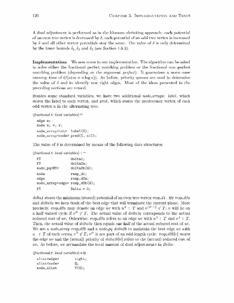
120 Chapter 3. Implementation and TestsA dual adjustment is performed as in the blossom{shrinking approa h: ea h potentialof an even tree vertex is de reased by Æ, ea h potential of an odd tree vertex is in reasedby Æ and all other vertex potentials stay the same. The value of Æ is only determinedby the lower bounds Æ1; Æ2 and Æ3 (see Se tion 1.6.3).Implementation: We now ome to our implementation. The algorithm an be askedto solve either the fra tional perfe t mat hing problem or the fra tional non{perfe tmat hing problem (depending on the argument perfe t). It guarantees a worst{ aserunning{time of O(n(m + n logn)). As before, priority queues are used to determinethe value of Æ and to identify new tight edges. Most of the ideas presented in thepre eding se tions are reused.Besides some standard variables, we have two additional node arrays: label , whi hstores the label to ea h vertex, and pred , whi h stores the prede essor vertex of ea hodd vertex u in the alternating tree.hfra tional.t: lo al variablesi�edge e;node u, v, r;node_array<int> label(G);node_array<node> pred(G, nil);The value of Æ is determined by means of the following data stru tures:hfra tional.t: lo al variablesi+�NT delta1;NT delta2a;node_pq<NT> delta2b(G);node resp_d1;edge resp_d2a;node_array<edge> resp_d2b(G);NT Delta = 0;delta1 stores the minimum (stored) potential of an even tree vertex resp d1 . By resp d2aand delta2a we keep tra k of the best edge that will terminate the urrent phase. Morepre isely, resp d2a may denote an edge uv with u+ 2 T and vf?j+g 62 T ; v will lie ona half{valued y le if v? 62 T . The a tual value of delta2a orresponds to the a tualredu ed ost of uv . Otherwise, resp d2a refers to an edge uv with u+ 2 T and v+ 2 T .Then, the a tual value of delta2a then equals one half of the a tual redu ed ost of uv .We use a node array resp d2b and a node pq delta2b to maintain the best edge uv withu+ 2 T of ea h vertex v? 62 T ; v? is not part of an odd length y le. resp d2b[v℄ storesthe edge uv and the (a tual) priority of delta2b[v℄ refers to the (a tual) redu ed ost ofuv. As before, we a umulate the total amount of dual adjustments in Delta:hfra tional.t: lo al variablesi+�slist<edge> tight;slist<node> Q;node_slist T(G);

3.5 Constru ting Better Initial Solutions 121A list tight is used to olle t all edges that have re ently be ome tight and an thusbe used by the algorithm. Q and T are essentially used as in the single sear h treealgorithm of the blossom{shrinking approa h: Q stores all new even verti es, and Tkeeps all verti es that are part of the alternating tree.The overall stru ture of our algorithm is as follows.hfra tional.t: algorithmi�template< lass NT>int jump_start( onst ugraph &G, onst edge_array<NT> &w,node_array<NT> &pot, node_array<node> &mate,bool perfe t) {hfra tional.t: lo al variablesihfra tional.t: initializationiforall_nodes(r, G) {if (mate[r℄ || pred[r℄) ontinue;h lear priority queues, Q and tightipot[r℄ += Delta;T.append(r); Q.append(r);bool terminate = false;while (!terminate) {hs an all edges of verti es in Qiif (delta1 == Delta) {halternate step using best node of delta1 i}else if (!tight.empty()) {huse all tight edgesi}else {hdual adjustmentihextra t tight edgesi}}}hmat h all odd length y lesireturn free;}The initialization is simple: we ompute a greedy mat hing and label all verti es ap-propriately.hfra tional.t: initializationi�int free = greedy_mat hing(G, w, pot, mate, perfe t);if (free == 0) return free;forall_nodes(u, G)label[u℄ = (mate[u℄ ? unlabeled : even);Next, a phase is initiated for ea h free vertex r. We use the following onvention to

122 Chapter 3. Implementation and Testsdetermine the value x(Æ(u)) to a given vertex u:x(Æ(u)) = 8><>:0 when mate [u℄ = nil and pred [u℄ = nil ,12 when mate [u℄ = nil and pred [u℄ 6= nil ,1 when mate [u℄ 6= nil .For a half{valued odd length y le C we will set the pred [u℄ entry of ea h ver-tex u 2 C su h that the y le an be traversed following these entries, i.e. C =u; pred [u℄; pred [pred [u℄℄; : : : .At the beginning of ea h phase, delta1 and delta2a are reset and delta2b, Q and T aremade empty.h lear priority queues, Q and tighti�delta1 = delta2a = INFINITY(NT);delta2b. lear();Q. lear(); tight. lear();The free vertex r is added to T and entered into Q. Due to the status hange ofr, we have to adjust its potential by +Delta (see formula (2.3), Se tion 2.1); we donot maintain an o�set for ea h vertex, but instead adjust its potential when a status hange o urs. In a while loop, all edges in ident to verti es in Q are s anned as willbe explained below. Afterwards, we initiate an alternate step when the a tual valueof delta1 equals zero (this will only happen in the non{perfe t ase), or use the tightedges olle ted in tight to extend T . When neither ase applies, a dual adjustment isperformed.hdual adjustmenti�NT and2b = (delta2b.empty() ? \INFINITY(NT) : delta2b.prio(delta2b.find_min()));NT delta = leda_min(delta1, leda_min(delta2a, and2b));if (delta == INFINITY(NT) && perfe t) {mate.init(G, nil);return 0;}Delta = delta; // orresponds to Delta += (delta - Delta)When the a tual value of delta1 equals zero, we immediately resume the while loop.When delta2a has a tual value zero, the responsible edge resp d2a is appended to tight(resp d2a is the only element). The next step will terminate the phase; note that Q isempty. Otherwise, all new tight edges are retrieved from delta2b and added to tight .hextra t tight edgesi�if (delta1 == Delta) ontinue;else if (delta2a == Delta) {tight.append(resp_d2a);resp_d2a = nil;}else {while (!delta2b.empty() &&

3.5 Constru ting Better Initial Solutions 123(delta2b.prio(delta2b.find_min()) == Delta)) {u = delta2b.del_min();tight.append(resp_d2b[u℄);resp_d2b[u℄ = nil;}}Finally, the algorithm terminates with an optimal solution to the fra tional mat hingproblem. We alternately mat h and unmat h (xe 2 f0; 1g) the edges along all existingodd length y les to obtain the �nal mat hing. Exa tly one vertex per y le (whi h isu below) will be ome free.hmat h all odd length y lesi�forall_nodes(u, G)if (pred[u℄) {alternate_ y le(u, mate, pred);free++;}The fun tion alternate y le is easily de�ned as follows.hfra tional.t: helpersi�void alternate_ y le(node u, node_array<node> &mate,node_array<node> &pred) {node ur1 = pred[u℄;while ( ur1 != u) {mate[pred[ ur1℄℄ = ur1;mate[ ur1℄ = pred[ ur1℄;node h = pred[ ur1℄;pred[ ur1℄ = nil; ur1 = h;h = pred[ ur1℄;pred[ ur1℄ = nil; ur1 = h;}pred[u℄ = nil;}Starting with ur1 = pred [u℄, we traverse the odd length y le, alternately mat hingand unmat hing the edges along this y le by setting the mate and pred entries appro-priately.All remaining details will be �lled in subsequently.S anning New Even Verti es: As in the blossom{shrinking approa h, all edgesin ident to any vertex that has re ently be ome an even tree vertex need to be inspe ted.This is ne essary so as to maintain delta1 , delta2a as well as delta2b orre tly.hs an all edges of verti es in Qi�while (!Q.empty()) {u = Q.pop();NT pot_u = pot[u℄ - Delta;

124 Chapter 3. Implementation and Testsif (!perfe t) {htry to improve delta1 i}forall_adj_edges(e, u) {v = opposite(u, e);if (label[v℄ == odd) ontinue;NT pot_v = pot[v℄ - (((label[v℄ == even) && T.member(v)) ? Delta : 0);NT pi = pot_u + pot_v - w[e℄;if (pi == 0) {hadd edge e to tighti}else {hprune edgesiif ((label[v℄ == unlabeled) && mate[v℄) {hnew delta2b edge en ounteredi}else {hnew delta2a edge en ounteredi}}}}We ompute the a tual potential pot u for ea h even tree vertex u in Q. The a tualpotential of a vertex u will be determined as stated in Se tion 2.1 (formula (2.1)); theonly di�eren e is that no o�set exists.delta1 is only maintained in the non{perfe t mat hing ase.htry to improve delta1 i�if (pot_u < leda_min(delta1, delta2a) - Delta) {delta1 = pot_u + Delta;resp_d1 = u;if (delta1 == Delta) break;}All edges e = uv in ident to u are onsidered. When the adja ent vertex v of u is oddwe simply ontinue, sin e nothing has to be done. Otherwise, we ompute the a tualpotential pot v of v and the a tual redu ed ost pi of uv. When e is tight, i.e. pi equalszero, we add e to the list tight .hadd edge e to tighti�if ((label[v℄ == unlabeled) && mate[v℄) tight.append(e);else {tight. lear(); Q. lear();tight.append(e);break;}If we have en ountered a tight edge that will terminate the urrent phase, we pro eedas follows. Q and tight are emptied and e be omes the only element of tight ; we breakthe s anning pro edure.Otherwise, the a tual redu ed ost pi is larger than zero. As for our single sear h tree

3.5 Constru ting Better Initial Solutions 125algorithm of the blossom{shrinking approa h, we prune hopeless edges; i.e. edges whosestored priority in delta2a or delta2b ex eeds the minimum value of delta1 and delta2a .18hprune edgesi�#if !defined(_NO_PRUNING)if (label[v℄ == even && T.member(v)) {if (pi/2 + Delta >= leda_min(delta1, delta2a)) ontinue;}else if (pi + Delta >= leda_min(delta1, delta2a)) ontinue;#endifWhen v is an unlabeled vertex and does not lie on a half{valued y le, we he k whetheror not e is the new best edge for v. If it is, we set resp d2b[v℄ to e and store the (stored)redu ed ost of e in delta2b.hnew delta2b edge en ounteredi�if (delta2b.member(v)) {if (pi < delta2b.prio(v) - Delta) {delta2b.de rease_p(v, pi + Delta);resp_d2b[v℄ = e;}}else {delta2b.insert(v, pi + Delta);resp_d2b[v℄ = e;}When v is not of the kind above, we have dis overed a new edge for delta2a . A he k isperformed to determine whether e is the new best edge of delta2a ; if it is, delta2a andresp d2a are set appropriately. Note that pi must be halved in the ase where v is aneven labeled tree vertex.hnew delta2a edge en ounteredi�if ((label[v℄ == even) && T.member(v)) pi /= 2;if (pi < delta2a - Delta) {delta2a = pi + Delta;resp_d2a = e;}Alternate Step: Let us onsider the alternate step. The edges along the (evenlength) tree path from resp d1 towards the root r get alternately unmat hed andmat hed.halternate step using best node of delta1 i�alternate_path(resp_d1, label, mate, pred);destroy_tree(T, label, pot, mate, pred, Delta);label[resp_d1℄ = even;terminate = true;18De�ne the token NO PRUNING (#define NO PRUNING) to swit h o� this strategy.

126 Chapter 3. Implementation and TestsAfter this, T is destroyed and the phase terminates. Note that destroy tree will set thelabel of resp d1 to unlabeled . We therefore need to orre t it to even.We give the implementation details of the fun tion alternate path , whi h alternates theedge along the tree path starting with the given vertex u.hfra tional.t: helpersi+�void alternate_path(node u, node_array<int> &label,node_array<node> &mate, node_array<node> &pred) {node ur = u;node pre = nil, nxt;while ( ur) {if (label[ ur℄ == even) {nxt = mate[ ur℄;mate[ ur℄ = pre; ur = nxt;}else {pre = ur;mate[ ur℄ = pred[ ur℄;nxt = pred[ ur℄;pred[ ur℄ = nil; ur = nxt;}}}Following the path from u towards the root, the mate and pred entries are set appro-priately for ea h vertex on the path.The urrent alternating tree T is easily destroyed.hfra tional.t: helpersi+�template< lass NT>void destroy_tree(node_slist &T, node_array<int> &label, node_array<NT> &pot,node_array<node> &mate, node_array<node> &pred, NT Delta) {node v;while (!T.empty()) {v = T.pop();if (label[v℄ == even) pot[v℄ -= Delta;else {pot[v℄ += Delta;if (mate[v℄) pred[v℄ = nil; // only for verti es not on y le}label[v℄ = unlabeled;}}Ea h vertex v is removed from T . Depending on the status of v, its potential pot [v℄needs to be adjusted as stated in formula (2.3). Moreover, when u is an odd vertex,pred [u℄ is set to nil ; however, it is ru ial that pred [u℄ is not set to nil when u is part

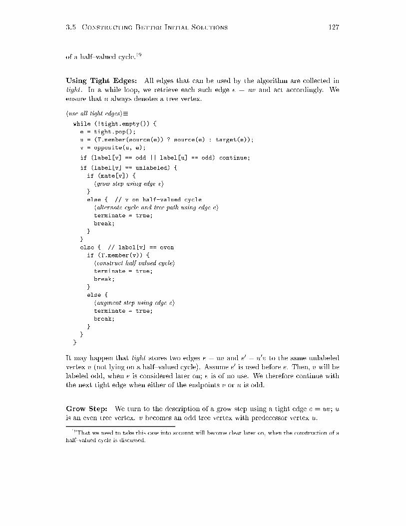
3.5 Constru ting Better Initial Solutions 127of a half{valued y le.19Using Tight Edges: All edges that an be used by the algorithm are olle ted intight . In a while loop, we retrieve ea h su h edge e = uv and a t a ordingly. Weensure that u always denotes a tree vertex.huse all tight edgesi�while (!tight.empty()) {e = tight.pop();u = (T.member(sour e(e)) ? sour e(e) : target(e));v = opposite(u, e);if (label[v℄ == odd || label[u℄ == odd) ontinue;if (label[v℄ == unlabeled) {if (mate[v℄) {hgrow step using edge ei}else { // v on half-valued y lehalternate y le and tree path using edge eiterminate = true;break;}}else { // label[v℄ == evenif (T.member(v)) {h onstru t half valued y leiterminate = true;break;}else {haugment step using edge eiterminate = true;break;}}}It may happen that tight stores two edges e = uv and e0 = u0v to the same unlabeledvertex v (not lying on a half{valued y le). Assume e0 is used before e. Then, v will belabeled odd, when e is onsidered later on; e is of no use. We therefore ontinue withthe next tight edge when either of the endpoints v or u is odd.Grow Step: We turn to the des ription of a grow step using a tight edge e = uv ; uis an even tree vertex. v be omes an odd tree vertex with prede essor vertex u.19That we need to take this ase into a ount will be ome lear later on, when the onstru tion of ahalf{valued y le is dis ussed.

128 Chapter 3. Implementation and Testshgrow step using edge ei�label[v℄ = odd;pred[v℄ = u;pot[v℄ -= Delta;T.append(v);delta2b.del(v);resp_d2b[v℄ = nil;The potential of v is adjusted a ording to its status hange. We delete the best edgedata for v from delta2b and resp d2b.The mate m of v is also added to T . m be omes an even tree vertex and is added toQ. Its entry in delta2b as well as in resp d2b is deleted.hgrow step using edge ei+�node m = mate[v℄;label[m℄ = even;pot[m℄ += Delta;T.append(m);Q.append(m);delta2b.del(m);resp_d2b[m℄ = nil;Alternate Cy le and Tree Path: We next onsider the ase where e = uv is atight edge with u+ 2 T , v? 62 T and v lies on a half{valued y le C. We alternatelyunmat h and mat h the edges along C starting at v; the fun tion alternate y le toa hieve this has already been presented. v will afterwards be free.halternate y le and tree path using edge ei�alternate_ y le(v, mate, pred);alternate_path(u, label, mate, pred);mate[u℄ = v;mate[v℄ = u;destroy_tree(T, label, pot, mate, pred, Delta);free--;We alternately unmat h and mat h the edges along the tree path from u to r allingalternate path and �nally mat h u and v with ea h other. T is subsequently destroyed.Constru ting a Half{Valued Cy le: When a tight edge e = uv is of the kindu+ 2 T and v+ 2 T , we pro eed as follows. We determine the lowest ommon an estorvertex l a of u and v by alling the fun tion seek l a . Starting in l a the edges along thetree path are alternately unmat hed and mat hed by the fun tion alternate path (l abe omes free). Then, a new half{valued y le C = (l a ; : : : ; u; v; : : : ; l a) is onstru ted, alling onstru t y le. Finally, the tree T is destroyed and free is de reased by one,sin e the root r is now mat hed.

3.5 Constru ting Better Initial Solutions 129h onstru t half valued y lei�node l a;seek_l a(u, v, l a, mate, pred, P1, P2, lo k);alternate_path(l a, label, mate, pred); onstru t_ y le(u, v, l a, mate, pred);destroy_tree(T, label, pot, mate, pred, Delta);free--;The lowest ommon an estor vertex is determined in lo k{step fashion as dis ussedbefore. We therefore additionally introdu e the following lo al data stru tures.hfra tional.t: lo al variablesi+�double lo k = 0;node_array<double> P1(G, 0);node_array<double> P2(G, 0);The determination of the lowest ommon an estor vertex is a hieved as follows.hfra tional.t: helpersi+�void seek_l a(node u, node v, node &l a,node_array<node> &mate, node_array<node> &pred,node_array<double> &P1, node_array<double> &P2,double &lo k) {node ur1 = u, ur2 = v;P1[ ur1℄ = P2[ ur2℄ = ++lo k;while ((P1[ ur2℄ != lo k) && (P2[ ur1℄ != lo k) &&(mate[ ur1℄ || mate[ ur2℄)) {if (mate[ ur1℄) { ur1 = pred[mate[ ur1℄℄;P1[ ur1℄ = lo k;}if (mate[ ur2℄) { ur2 = pred[mate[ ur2℄℄;P2[ ur2℄ = lo k;}}if (P1[ ur2℄ == lo k) // ur2 is l al a = ur2;else if (P1[ ur1℄ == lo k) // ur1 is l al a = ur1;else l a = nil;}We follow the two tree paths from u and v towards the root r. All even verti es onthe path from u to r are marked by lo k using the node array P1 and all even verti eson the path from v to r are marked by lo k using the node array P2 . When eitherP1 [ ur2 ℄ or P2 [ ur1 ℄ equals lo k , the lowest ommon an estor l a has been found.We now dis uss the details of the half{valued y le onstru tion. The idea is simple.Let pu and pv denote the two tree paths from u and v to the l a vertex, respe tively.First, the pred entries of all verti es along pu are set su h that they represent thereversed path of pu. Then, the pred entries of all verti es along pv are set su h that

130 Chapter 3. Implementation and Teststhey represent pv itself. Finally, we set pred [u℄ to v and obtain the representation of Cas desired.hfra tional.t: helpersi+�void onstru t_ y le(node u, node v, node l a,node_array<node> &mate, node_array<node> &pred) {node ur1 = u, ur2 = v;while ( ur1 != l a) {// set pred data to reversed tree path; delete mate entriesnode h = mate[ ur1℄;mate[ ur1℄ = nil; ur1 = pred[h℄;pred[h℄ = mate[h℄;mate[h℄ = nil;pred[ ur1℄ = h;}while ( ur2 != l a) {// set pred data to tree path; delete mate entriesnode h = mate[ ur2℄;pred[ ur2℄ = mate[ ur2℄;mate[ ur2℄ = nil;mate[h℄ = nil; ur2 = pred[h℄;}pred[u℄ = v;}Augment Step: The only detail that has not been presented yet is how to performan augment step for a tight edge e = uv with u+ 2 T and v+ 62 T . We �rst alternatelyunmat h and mat h the edges along the tree path from u to the root vertex r (u be omesfree). Thereafter, u and v are mat hed with ea h other (v be omes unlabeled), the treeT is destroyed and free is de reased by 2.haugment step using edge ei�alternate_path(u, label, mate, pred);mate[u℄ = v;mate[v℄ = u;label[v℄ = unlabeled;destroy_tree(T, label, pot, mate, pred, Delta);free -= 2;This on ludes the dis ussion of all the details involved in the onstru tion of an initialmat hing M and the vertex potentials by solving the fra tional mat hing problem.3.6 Experimental ResultsWe performed several experiments in order to rate the pra ti al eÆ ien y of our algo-rithms. The omparisons we made are as follows.

3.6 Experimental Results 131(1) Comparison of di�erent strategies: single sear h tree approa h with and with-out pruning strategy, multiple sear h tree approa h with and without providentstrategy.(2) Comparison of the single sear h tree approa h with the multiple sear h tree ap-proa h, and the e�e t of using di�erent heuristi s.(3) Comparison of our multiple sear h tree approa h with other mat hing algorithmsavailable in LEDA.(4) Comparison of our multiple sear h tree approa h with the urrently most eÆ ientalgorithm, Blossom IV, of Cook and Rohe [CR97℄.In this se tion we will dis uss the results of these omparisons. In summary, they revealthe eÆ ien y of our algorithms in pra ti e. We wish to state that our multiple sear htree approa h is (at least) ompetitive to Blossom IV: so far, we have not en ounteredan instan e on whi h our algorithm is inferior (if the omparison is fair, as we areabout to explain). However, we would like to leave the de ision on whether or not ouralgorithm is superior to Blossom IV to the reader. We de ided so, due to the fa t thatBlossom IV uses a so{ alled pri e and repair strategy for omplete geometri instan esthat we have not yet implemented for our algorithm. The pri e and repair strategysigni� antly improves the running{time of Blossom IV on these instan es. Due to thela k of a similar strategy for our algorithm, the omparisons on omplete geometri instan es are regarded to be not quite fair.Experimental Setting: We experimented with three kinds of instan es: Delaunayinstan es, (sparse and dense) random instan es and omplete geometri instan es.For the Delaunay instan es we hose n random points in the unit square and omputedthe Delaunay triangulation (using the LEDA Delaunay implementation). The edgeweights orrespond to the Eu lidean distan es s aled to integers in the range [0; : : : ; 216).Delaunay graphs are known to ontain perfe t mat hings (see Dillen ourt [Dil90℄).For the random instan es we reated random graphs with n verti es. The number ofedges for sparse graphs was hosen as m = �n for small values of �, � � 10.The number of edges for dense graphs is about 20%, 40% and 60% of the density of a omplete graph, i.e. m = dn(n� 1)=2, with d 2 f0:2; 0:4; 0:6g.Complete geometri instan es were indu ed by n random points in a n� n square andtheir Eu lidean distan e.The running{times of all our experiments are stated in se onds and are the average oft = 5 runs, unless stated otherwise. All experiments were performed on a Sun UltraSpar , 333 Mhz.Di�erent Strategies We dis uss the in uen e of the usage of di�erent strategies forea h approa h. The omparisons were made on sparse random graphs with n verti esand a �xed � = 10. Both algorithms omputed a maximum{weight mat hing; thegreedy heuristi was used.

132 Chapter 3. Implementation and TestsThe single sear h tree approa h (SST) has been implemented to use a pruning strategyby default. Table 3.1 implies this to be reasonable.n � SST+pru� SST+pru+ t10000 6 37:42 28:17 520000 6 125:95 99:60 540000 6 428:78 364:67 5Table 3.1: E�e t of pruning strategy for single sear h tree algorithm (SST).We ompared the single sear h tree algorithm using the pruning strategy (SSTpru+)with the single sear h tree algorithm not using the pruning strategy (SSTpru�). Therunning{time of the single sear h tree algorithm is onsiderably improved using thepruning strategy. Re all that the pruning strategy is also implemented for the fra tionalmat hing heuristi .For the multiple sear h tree approa h, the user may hoose between the providentand the non{provident strategy. As mentioned previously, the non{provident strategy(MSTpro�) seems to us to be slightly superior to the provident strategy (MSTpro+).However, the di�eren es are negligible, as indi ated in Table 3.2.n � MST+pro+ MST+pro� t10000 6 13:14 12:89 520000 6 29:20 28:59 540000 6 67:02 66:01 5Table 3.2: E�e t of non{provident strategy for multiple sear h tree algorithm (MST).In the subsequent omparisons, we will always use the strategies that are hosen bydefault. That is, the single sear h tree approa h as well as the fra tional mat hingheuristi use the pruning strategy, and the multiple sear h tree approa h implementsthe non{provident strategy.Single Sear h Tree vs. Multiple Sear h Tree Approa h: We ompared thesingle sear h tree approa h (SST) to the multiple sear h tree approa h (MST) usingdi�erent heuristi s. The results are given in Table 3.3.n SST� MST� SST+ MST+ GY SST� MST� FM t10000 37:01 6:27 24:05 4:91 0:13 5:79 3:20 0:40 520000 142:93 14:81 89:55 11:67 0:24 18:54 8:00 0:83 540000 593:58 31:53 367:37 25:51 0:64 76:73 17:41 1:78 5Table 3.3: SST vs. MST algorithm and e�e t of greedy and fra tional mat hing heuristi s.Both algorithms omputed a maximum{weight perfe t mat hing on Delaunay instan eswith n verti es. Either no heuristi (�), the greedy heuristi (+) or the fra tionalmat hing heuristi (�) was used. The time needed to onstru t a greedy or a fra tionalmat hing is given in olumns GY and FM , respe tively.

3.6 Experimental Results 133The fra tional mat hing heuristi is omputationally more intensive than the greedyheuristi . However, the fra tional mat hing heuristi improves the overall running{time of both algorithms signi� antly. We draw attention to the fa t that the di�eren ebetween the two heuristi s is more pronoun ed for the single sear h tree approa h. Themultiple sear h tree approa h is superior to the single sear h tree approa h.p qWe will attempt to give an interpretation for the better running{time performan e of the mul-tiple sear h tree approa h. We take a loser look at the number of dual adjustments that wereperformed during the ourse of the algorithms. Our algorithms an be asked to output ertainstatisti al information (not do umented in the pre eding se tions). We give a sample outputbelow.MST SST----------------------------------------------------- -----------------------------------------------------INIT: 0.28 se . INIT: 0.19 se .MATCHING: 14.40 se . MATCHING: 40.07 se .EXTRACT: 0.14 se . EXTRACT: 0.12 se .CHECKER: 0.23 se . CHECKER: 0.22 se .----------------------------------------------------- -----------------------------------------------------ADJUSTMENTS: 7663 ADJUSTMENTS: 13428SCAN: 29295 5.91 se . (avg. 0.20 mse .) SCAN: 81237 4.93 se . (avg. 0.06 mse .)GROW: 16593 0.44 se . (avg. 0.03 mse .) GROW: 62265 0.86 se . (avg. 0.01 mse .)SHRINK: 8 0.00 se . (avg. 0.00 mse .) SHRINK: 155 0.11 se . (avg. 0.71 mse .)EXPAND: 5 0.00 se . (avg. 0.00 mse .) EXPAND: 148 0.16 se . (avg. 1.08 mse .)ALTERNATE: 43 0.00 se . (avg. 0.00 mse .) ALTERNATE: 258 0.21 se . (avg. 0.81 mse .)AUGMENT: 4983 7.40 se . (avg. 1.49 mse .) AUGMENT: 4983 0.44 se . (avg. 0.09 mse .)DESTROY TREE: 10000 6.54 se . (avg. 0.65 mse .) DESTROY TREE: 5241 0.57 se . (avg. 0.11 mse .)----------------------------------------------------- -----------------------------------------------------TOTAL TIME (without he king): 14.84 se . TOTAL TIME (without he king): 40.39 se .Both algorithms omputed a maximum{weight mat hing on the same random instan e withn = 10000, m = 60000 and edge weights in the range [0; : : : ; 216). No heuristi was used.We �rst of all observe that the multiple sear h tree approa h needs to perform fewer dualadjustments than the single sear h tree approa h. This is to be expe ted; we onsider the rateof hange �f of the dual obje tive value. For the single sear h tree approa h we observedthat �f = �Æ, when a dual adjustment is performed by Æ ( f. dis ussion on page 30). In themultiple sear h tree approa h, however, we have a de rease by Æ for ea h existing tree. That is,�f = �tÆ, where t refers to the number of alternating trees that urrently exist when a dualadjustment is performed.Further, it seems to us that the single sear h tree approa h needs to initiate needless steps, sin eit is for ed to sear h from a �xed free vertex. Note, for example, that the average number ofs an, alternate, grow, shrink and expand steps per augmentation di�ers drasti ally. However,this statement is vague.x yIn the omparisons that follow, we hose the multiple sear h tree approa h using thefra tional mat hing heuristi (MST�) as the anoni al implementation.Comparisons to Mat hing Algorithms in LEDA: LEDA provides an algorithmfor ea h of the four variants of the mat hing problem introdu ed in Chapter 1: amaximum{ ardinality bipartite mat hing algorithm (BCM), a maximum{ ardinalitymat hing algorithm (GCM), a maximum{weight bipartite mat hing algorithm (BWM)and a maximum{weight mat hing algorithm (GWM). The theoreti al running{time ofthe algorithms are as follows: O(pnm) for BCM, O(nm�(n;m)) for GCM (� denotesthe inverse A kermann fun tion), O(n(m + n logn)) for BWM and O(n3) for GWM.For a detailed des ription of the underlying algorithms and their implementations seethe book by Mehlhorn and N�aher [MN99, Chapter 7℄.

134 Chapter 3. Implementation and TestsWe ompared our MST algorithm to ea h of the algorithms. The tests were performedon sparse random graphs with n verti es and �n edges. In the ardinality ases, unitweights (we = 1) were used by our algorithm. The results an be seen in Table 3.4.Due to the time intensity of GWM, the omparisons were made on small instan es onlywith n = 10000.n � BCM MST� GCM MST� BWM MST� GWM MST� t10000 4 0:73 1:14 0:55 1:94 3:67 1:57 585:43 1:44 510000 6 0:92 0:67 0:50 0:91 7:81 3:95 883:66 3:96 510000 8 1:28 0:74 0:45 1:18 9:82 6:62 897:81 6:25 520000 4 1:81 2:69 1:42 5:19 9:30 3:31 � 3:42 520000 6 2:23 1:61 1:42 5:06 29:64 11:05 � 10:05 520000 8 3:06 1:65 1:29 2:56 35:62 18:05 � 18:53 540000 4 5:52 8:04 4:26 9:19 24:45 8:39 � 8:23 540000 6 5:92 4:54 3:86 14:10 109:35 32:50 � 30:22 540000 8 7:41 4:31 3:66 9:69 128:66 51:13 � 56:46 5Table 3.4: Comparison of our MST algorithm to the mat hing algorithms available in LEDA.We draw attention to the fa t that, for bipartite instan es, our algorithm is ompetitivewith the spe ialized algorithms in LEDA. In the bipartite ase, the fra tional mat hingheuristi will always ompute an optimal mat hing. That is, MST essentially redu esto the fra tional mat hing algorithm dis ussed in the pre eding se tion.Blossom IV: The Blossom IV algorithm of Cook and Rohe [CR97℄ is the most ef-� ient ode urrently available for weighted perfe t mat hings in general graphs. TheeÆ ien y of Blossom IV is revealed in two papers:(1) In [CR97℄ Blossom IV is ompared to the implementation of Applegate andCook [App93℄. It is shown that Blossom IV is substantially faster.(2) In [App93℄ the Applegate and Cook implementation is ompared to other imple-mentations. The authors show that their ode is superior to all other odes.Blossom IV an be asked to run either a single sear h tree approa h, a multiple sear htree approa h or a re�nement of the multiple sear h tree approa h alled the variableÆ approa h. In the variable Æ approa h, ea h alternating tree Tri hooses its own dualadjustment value Æri so as to maximize the de rease in the dual obje tive value. Aheuristi is used to make these hoi es, sin e the determination of optimum Æri 's wouldbe too ostly. The experiments in [CR97℄ show that the variable Æ approa h is superiorto the other approa hes in pra ti e.We ompared our MST algorithm to the multiple sear h tree approa h (B4) as well asto the variable Æ approa h (B4var) of Blossom IV. Blossom IV (B4 and B4var) also usesa fra tional mat hing heuristi to ompute an initial mat hing (indi ated by �).Delaunay Instan es: We give the experiments on Delaunay instan es with n verti esin Table 3.5.

3.6 Experimental Results 135n B4� B4�var MST� t10000 73:57 4:11 3:37 520000 282:20 12:34 7:36 540000 1176:58 29:76 15:84 5Table 3.5: MST algorithm vs. Blossom IV (B4 and B4var) on Delaunay instan es.Observe that the variable Æ approa h (B4var) is signi� antly faster than the multi-ple sear h tree approa h (B4). Our MST algorithm is ompetitive to the variable Æapproa h B4var.Asymptoti s: In Table 3.6 we ompared Blossom IV to our MST approa h on ran-dom instan es; we varied n for a �xed � = 6.n � B4� B4�var MST� t10000 6 20:94 18:03 3:51 520000 6 82:96 53:87 9:97 540000 6 194:48 177:28 29:05 5Table 3.6: MST algorithm vs. Blossom IV (B4 and B4var) on random instan es.Both algorithms, B4var and MST, seem to grow less than quadrati ally as a fun tionin n. B4var takes about six times as long as our multiple sear h tree approa h MST. InTable 3.7 we additionally varied �.n � B4� B4�var MST� t10000 6 20:90 20:22 3:49 510000 8 48:50 22:83 5:18 510000 10 37:49 30:78 5:41 520000 6 96:34 54:08 10:04 520000 8 175:55 89:75 12:20 520000 10 264:80 102:53 15:06 540000 6 209:84 202:51 29:27 540000 8 250:51 249:83 36:18 540000 10 710:08 310:76 46:57 5Table 3.7: MST algorithm vs. Blossom IV (B4 and B4var) on random instan es.A log{log plot indi ating the asymptoti s of Blossom IV (B4var) and our MST algorithmon random instan es (� = 6) is depi ted in Figure 3.2.In uen e of Edge Weights: Table 3.8 shows the in uen e of edge weights on therunning{time. We took random instan es with m = 4n edges and random edge weightsin the range [1; : : : ; b℄ and varied b.

136 Chapter 3. Implementation and TestsMST�B4�var

n

se .

32000016000080000400002000010000

1000100101Figure 3.2: Asymptoti s of MST algorithm and Blossom IV (B4var) on random instan es.n � b B4� B4�var MST� t10000 40000 1 3:98 3:99 0:85 110000 40000 10 2:49 3:03 2:31 110000 40000 100 3:09 3:10 2:58 110000 40000 1000 17:41 8:40 2:91 110000 40000 10000 13:69 11:91 2:78 110000 40000 100000 12:06 11:20 2:69 1Table 3.8: MST algorithm vs. Blossom IV (B4 and B4var). In uen e of edge weights.Both B4 and B4var are sensitive to di�erent edge weights. Their running{time signif-i antly depends on the range of hosen edge weights. The running{time of our MSTalgorithm is stable (ex ept for the unweighted ase (b = 1), whi h is simpler).p qWe attempt an explanation. When the range of edge weights is small, a single dual adjustmentis more likely to produ e more than one tight edge. In addition to or as a onsequen e of this,it seems to us that the number of dual adjustments needed to ompute an optimal mat hing issmaller. Table 3.9 indi ates that this assumption is in fa t true. We re orded the number ofdual adjustments needed by Blossom IV (B4var) and our MST algorithm.n � b B4�var MST� t10000 4 1 0 0 110000 4 10 2094 2076 110000 4 100 5269 5101 110000 4 1000 7487 7091 110000 4 10000 8063 7877 110000 4 100000 8491 8134 1Table 3.9: MST algorithm vs. Blossom IV (B4 and B4var). Number of dual adjustments.

3.6 Experimental Results 137Sin e Blossom IV needs time O(n) to perform a dual adjustment, whereas our implementationneeds time O(m logn) for all dual adjustments in a phase, our MST algorithm is less harmedwhen the edge weights are hosen from a large range.Observe that, although the variable Æ approa h (B4var) of Blossom IV was used, our algorithmneeds less dual adjustments.x yVarian e: Table 3.10 gives information about the varian e in running{time of Blos-som IV (B4var) and our MST algorithm. For ea h algorithm the best, worst and averagetime of �ve random instan es, with n verti es and � = 6, is given. The u tuation seemsto be about the same for the B4var and the MST algorithm.n � B4�var MST� tbest worst average best worst average10000 6 16:88 20:03 18:83 3:34 4:22 3:78 520000 6 49:02 60:74 55:15 9:93 11:09 10:30 540000 6 162:91 198:11 180:88 25:13 32:24 29:09 5Table 3.10: MST algorithm vs. Blossom IV (B4var) on random instan es. Varian e.Dense Random Instan es: The experiments suggest that our MST algorithm issuperior to B4var on sparse instan es. Table 3.11 shows the running{time on denseinstan es with n verti es and about 20%, 40% and 60% density. Our MST algorithmis ompetitive to B4var on these instan es as well.n m B4� B4�var MST� t1000 100000 6:97 5:84 1:76 51000 200000 16:61 11:35 3:88 51000 300000 18:91 18:88 5:79 52000 200000 46:71 38:86 8:69 52000 400000 70:52 70:13 16:37 52000 600000 118:07 115:66 23:46 54000 400000 233:16 229:51 42:32 54000 800000 473:51 410:43 92:55 54000 1200000 523:40 522:52 157:00 5Table 3.11: Comparison of MST algorithm to Blossom IV (B4 and B4var). Dense graphs.Complete Random Instan es and Pri e and Repair: Blossom IV provides aso{ alled pri e and repair heuristi for omplete geometri instan es. The instan es areimpli itly represented by a set of points in an n�n square (the edge weights orrespondto the Eu lidean distan e). Using the pri e and repair strategy signi� antly improvesthe running{time of Blossom IV on these instan es. We have not yet implementedsu h a heuristi for our algorithm. We ompared our MST algorithm to Blossom IVon omplete geometri instan es (B4var did not and B4parvar did use the pri e and repairstrategy). Our algorithm requires an expli it representation of the underlying graphand we thus were only able to experiment with rather small instan es. The results arepresented in Table 3.12.

138 Chapter 3. Implementation and Testsn B4�var B4�parvar MST� t1000 37:01 0:43 24:05 52000 225:93 1:10 104:51 54000 1789:44 4:33 548:19 5Table 3.12: MST algorithm vs. Blossom IV (B4var and B4parvar ). E�e t of pri e and repair.The idea underlying the pri e and repair heuristi is simple. Instead of running thealgorithm on the omplete set of edges, the pri e and repair heuristi starts with asparse subgraph. On e an optimum weighted mat hing is omputed for the sparsesubgraph a he k is performed to determine whether or not the omputed mat hing isalso optimum for the omplete graph. This is what is alled pri ing. Some of the edgeshaving negative redu ed ost are added to the urrent graph, with the mat hing andthe potentials being modi�ed su h that all pre onditions of the mat hing algorithm aresatis�ed. The algorithm is resumed so as to repair the mat hing for the urrent graph.This pro ess is repeated until the obtained mat hing is optimum for the omplete graph.There are several natural hoi es for the sele tion of the sparse subgraph. For example,a minimum{weight mat hing will have a natural tenden y to avoid heavy edges. Thus,taking the k lightest edges in ident to any vertex seems to be a reasonable hoi e. Infa t, this was the way Applegate and Cook [App93℄ onstru ted the initial subgraph(they alled it the k{nearest neighbour graph). Another hoi e, proposed by Cookand Rohe [CR97℄, is to use the Delaunay triangulation of the point set as the initialsubgraph. For more extensive sour es related to the pri e and repair strategy see Derigsand Metz [DM91℄, Applegate and Cook [App93℄ and Cook and Rohe [CR97℄.`Worse{ ase' Instan es for Blossom IV: A demanding task would be to imple-ment a generator, whi h onstru ts instan es that for e either algorithm, i.e. our MSTor the Blossom IV algorithm, into its worst ase. Random graphs tend to be rathersimple instan es; during the performan e of our experiments, for example, many ran-dom instan es o urred that had been solved almost optimal by the fra tional mat hingheuristi . So far, we have not been able to generate worst{ ase instan es for either al-gorithm. However, we wish to on lude this se tion with two `worse{ ase' instan esthat demonstrate the superiority of our algorithm to Blossom IV.The �rst `worse{ ase' instan e for Blossom IV is simply a hain. We onstru ted a hain having 2n verti es and 2n � 1 edges. The edge weights along the hain werealternately set to 0 and 2 (the edge weight of the �rst and last edge equals 0). BlossomIV (B4var) and our MST algorithm were asked to ompute a maximum{weight perfe tmat hing. Note that the fra tional mat hing heuristi will always ompute an optimalsolution on instan es of this kind. Table 3.13 shows the results.2n B4�var MST� t10000 94:75 0:25 120000 466:86 0:64 140000 2151:33 2:08 1Table 3.13: Comparison of MST algorithm to Blossom IV (B4var) on hains.

3.6 Experimental Results 139The running{time of Blossom IV grows more than quadrati ally (as a fun tion of n),whereas the running{time of our MST algorithm grows about linearly with n. Wepresent our argument as to why this is to be expe ted. First of all, the greedy heuristi will mat h all edges having weight 2; the two outer verti es remain unmat hed. Ea halgorithm will then have to perform O(n) dual adjustments so as to obtain the opti-mum mat hing. A dual adjustment takes time O(n) for Blossom IV (ea h potentialis expli itly updated), whereas it takes O(1) for our MST algorithm. Thus, BlossomIV will need time O(n2) for all these adjustments and, on the other hand, the timerequired by our MST algorithm will be O(n). The idea of testing both algorithms onthis kind of hains is due to Kurt Mehlhorn (personal ommuni ation).Another `worse{ ase' instan e for Blossom IV o urred in VLSI{Design having n =151780 verti es and m = 881317 edges. Kindly, Andreas Rohe made this instan eavailable to us. We ompared the Blossom IV algorithms (B4 and B4var) to our MSTalgorithm. We ran our algorithm with the greedy heuristi (MST+) as well as with thefra tional mat hing heuristi (MST�). The results are given in Table 3.14.n m B4� B4�var MST+ MST� t151780 881317 200019:74 200810:35 3172:70 5993:61 1(332:01) (350:18) (5:66) (3030:35)Table 3.14: Comparison of MST algorithm to Blossom IV (B4var) on boese.edg instan e.The se ond row states the times that were needed by the heuristi s. Observe that bothBlossom IV algorithms need more than two days to ompute an optimum mat hing,whereas our algorithm solves the same instan e in less than an hour. For our MSTalgorithm the fra tional mat hing heuristi did not help at all on this instan e: to ompute a fra tional mat hing took almost as long as omputing an optimum mat hingfor the original graph (using the greedy heuristi ).

Open ProblemsWe have des ribed a priority queue based O(nm log n) algorithm of Edmonds' blossom{shrinking approa h. Two implementations, a single sear h tree and a multiple sear htree algorithm, were presented. The additional programming expenditure for the mul-tiple sear h tree algorithm turned out to be well worth the e�ort when eÆ ien y inpra ti e is onsidered.Our multiple sear h tree algorithm is ompetitive with the most eÆ ient known im-plementation, Blossom IV, due to Cook and Rohe [CR97℄. Blossom IV implementsa re�nement of a multiple sear h tree approa h, alled the variable Æ approa h, andonly requires simple data stru tures. We an thus provide an aÆrmative answer tothe question whether or not sophisti ated data stru tures su h as on atenable priorityqueues help in pra ti e.Our resear h raises several questions. (1) The variable Æ algorithm is substantially fasterthan the other algorithms of Blossom IV. Would it be possible to integrate the variableÆ approa h into a priority queue based O(nm logn) algorithm? Moreover, it wouldbe interesting to see if an O(nm logn) variable Æ algorithm will improve the pra ti aleÆ ien y as dramati ally as for Blossom IV. (2) A pri e and repair strategy is worth onsidering for the O(nm log n) algorithm as well. We expe t that su h a strategy willimprove the running{time of our algorithm on dense and omplete instan es tremen-dously. (3) As previously mentioned, a generator of instan es for ing either algorithminto its worst ase would be of use. (4) Re ently, Stefan N�aher (personal ommu-ni ation) observed that using a stati variant of the graph data stru ture in LEDA( urrently, we use a dynami graph data stru ture) improves the overall running{timeof other graph algorithms by a fa tor of about two. Most likely, a similar e�e t anbe a hieved for our algorithm too. (5) Our fra tional mat hing heuristi also uses pri-ority queue data stru tures. So far, however, it only implements a single sear h treeapproa h. We believe that a fra tional mat hing heuristi based on the multiple sear htree approa h would further improve the running{time. Possibly, this would also resultin a more eÆ ient algorithm for bipartite mat hing problems. (6) At the end of Chap-ter 1, we (very roughly) sket hed the ideas underlying an O(n(m+ n log n)) approa h.Although we doubt that an eÆ ient implementation of this approa h is possible, it isworth attempting to falsify our hypothesis.

141

Bibliography[ADK+00℄ E. Althaus, D. Du hier, A. Koller, K. Mehlhorn, J. Niehren, and S. Thiel.An eÆ ient algorithm for the dominan e problem. Submitted, 2000.[AE85℄ J. Ar�aoz and J. Edmonds. A ase of non{ onvergent pivoting in assignmentproblems. Dis rete Appl. Math., 11:95{102, 1985.[AHU74℄ A. V. Aho, J. E. Hop roft, and J. D. Ullmann. The design and analysis of omputer algorithms. Addison-Wesley, 1974.[AMO93℄ R. K. Ahuja, T. L. Magnanti, and J. B. Orlin. Network ows : theory,algorithms and appli ations. Prenti e Hall, 1993.[App93℄ W. Applegate, D. and Cook. Solving large-s ale mat hing problems. InDavid S. Johnson and Catherine C. M Geo h, editors, Network Flows andMat hings, volume 12 of DIMACS Series in Dis rete Mathemati s and The-oreti al Computer S ien e, pages 557{576, Providen e, RI, 1993. Ameri anMathemati al So iety.[BBD83℄ M. O. Ball, L. D. Bodin, and R. Dial. A mat hing based heuristi fors heduling mass transit rews and vehi les. Transportation S ien e, 17:4{31, 1983.[Bel94℄ C. E. Bell. Weighted mat hing with vertex weights: an appli aton tos heduling training sessions in NASA spa e shuttle o kpit simulators. Eu-ropean Journal of Operational Resear h, 73:443{449, 1994.[Ber57℄ C. Berge. Two theorems in graph theory. In Pro eedings of the NationalA ademy of S ien es, volume 43, pages 842{844, USA, 1957.[Ber58℄ C. Berge. Sur le ouplage maximum d�un graphe. C. R. A ad. S i. ParisS�er. I Math., 247:258{259, 1958.[Bir46℄ G. Birkho�. Tres observa iones sobre el algebra lineal. Rev. Fa . Ci. Exa -tas, Puras y Apli adas Univ. Na . Tu uman, Ser. A 5:147{151, 1946.[BS00℄ R. Beier and J. Sibeyn. A powerful heuristi for telephone gossiping. Te h-ni al report, Max{Plan k Institut f�ur Informatik, 2000.[BT97℄ D. Bertsimas and J. N. Tsitsiklis. Introdu tion to linear optimization, vol-ume 6. Athena S ienti� , 1997.143

144 Bibliography[CCPS98℄ W. J. Cook, W. H. Cunningham, W. R. Pulleyblank, and A. S hrijver.Combinatorial optimization. Wiley-inters ien e series in dis rete mathe-mati s and optimization. Wiley, 1st edition, 1998.[Chr76℄ N. Christo�des. Worst{ ase analysis of a new heuristi for the travellingsalesman problem. Te hni al report, Graduate S hool of Industrial Admin-istration, Carnegie{Mellon University, Pittsburgh, PA, 1976.[Chv83℄ V. Chv�atal. Linear programming. W. H. Freeman and Co., 1983.[CLR92℄ T. H. Cormen, C. E. Leiserson, and R. L. Rivest. Introdu tion to algorithms.The MIT ele tri al engineering and omputer s ien e series. MIT Press, 6thprinting edition, 1992.[CR97℄ W. Cook and A. Rohe. Computing minimum{weight perfe t mat hings.Te hni al Report 97863, Fors hungsinstitut f�ur Diskrete Mathematik, Uni-versit�at Bonn, 1997.[Dil90℄ M. B. Dillen ourt. Toughness and delaunay triangulations. Dis rete andComputational Geometry, 5:575{601, 1990.[DM86℄ U. Derigs and A. Metz. On the use of optimal fra tional mat hings for solv-ing the (integer) mat hing problem. Mathemati al Programming, 36:263{270, 1986.[DM91℄ U. Derigs and A. Metz. Solving (large s ale) mat hing problems ombina-torially. Mathemati al Programming, 50:113{122, 1991.[DM92℄ U. Derigs and A. Metz. A mat hing{based approa h for solving deliv-ery/pi kup vehi le routing problem with time onstraints. Operations Re-sear h Spektrum, 14:91{106, 1992.[Edm65a℄ J. Edmonds. Maximum mat hing and a polyhedron with (0,1) verti es.Journal of Resear h of the National Bureau of Standards, 69B:125{130,1965.[Edm65b℄ J. Edmonds. Paths, trees and owers. Canadian Journal of Mathemati s,17:449{467, 1965.[FT87℄ M. L. Fredman and R. E. Tarjan. Fibona i heaps and their uses in improvednetwork optimization algorithms. Journal of the ACM, 34, 1987.[Gab74℄ H. N. Gabow. Implementation of algorithms for maximum mat hing andnonbipartite graphs. PhD thesis, Stanford University, 1974.[Gab85℄ H. N. Gabow. A s aling algorithm for weighted mat hing on general graphs.In 26th Annual Symposium on Foundations of Computer S ien e, pages 90{100. IEEE Computer So iety Press, O tober 1985.[Gab90℄ H. N. Gabow. Data stru tures for weighted mat hing and nearest ommonan estors with linking. In David Johnson, editor, Pro eedings of the 1stAnnual ACM-SIAM Symposium on Dis rete Algorithms (SODA '90), pages434{443, San Fran is o, CA, USA, January 1990. SIAM.

Bibliography 145[GGS89℄ H. N. Gabow, Z. Galil, and T. H. Spen er. EÆ ient implementation ofgraph algorithms using ontra tion. Journal of the ACM, 36, 1989.[GKT99℄ H. N. Gabow, H. Kaplan, and R. E. Tarjan. Unique maximum mat hingalgorithms. To appear in STOC, 1999.[GMG86℄ Z. Galil, S. Mi ali, and H. N. Gabow. An O(EV log V ) algorithm for �nd-ing a maximal weighted mat hing in general graphs. SIAM J. Computing,15:120{130, 1986.[GT91℄ H. N. Gabow and R. E. Tarjan. Faster s aling algorithms for general graphmat hing problems. Journal of the ACM, 38:815{853, 1991.[K�on16℄ D. K�onig. �Uber Graphen und ihre Anwendung auf Determinatentheorie undMengenlehre. Math. Ann., 77:453{465, 1916.[Law76℄ E. L. Lawler. Combinatorial Optimization: Networks and Matroids. Holt,Rinehart and Winston, New York, 1976.[LP86℄ L. Lov�asz and M. D. Plummer. Mat hing theory, volume 121/29 of North{Holland mathemati s studies. North{Holland, 1986.[Meh84℄ K. Mehlhorn. Data stru tures and algorithms. Volume 1: Sorting andsear hing, volume 1 of EATCS monographs on theoreti al omputer s ien e.Springer, 1984.[MN99℄ K. Mehlhorn and S. N�aher. LEDA : a platform for ombinatorial and geo-metri omputing. Cambridge University Press, 1999.[PS82℄ C. H. Papadimitriou and K. Steiglitz. Combinatorial optimization | algo-rithms and omplexity. Prenti e-Hall, 1982.[Pul95℄ W. R. Pulleyblank. Mat hings and extensions. In Ronald L. Graham,Martin Gr�ots hel, and L�aszl�o Lovasz, editors, Handbook of ombinatori s,volume 1, pages 179{232, Amsterdam, 1995. Elsevier.[RT81℄ E. M. Reingold and R. E. Tarjan. On a greedy heuristi for omplete mat h-ing. SIAM Journal of Computing, 10:676{681, 1981.[Tut47℄ W. T. Tutte. The fa torisation of linear graphs. J. London Math. So .,22:107{111, 1947.