weight estimation through frequency analysis - …223502/fulltext01.pdf · weight estimation...
TRANSCRIPT

Weight Estimation through Frequency Analysis
Hampus Johansson Nicklas Höglund
Fluid and Mechanical Engineering Systems
Master thesis Department of Management and Engineering (IEI)
LIU-IEI-TEK-A—09/00638—SE
Source: Semcon Informatic Graphic Solutions
Weight Estimation through Frequency Analysis
Thesis for the Degree of Master of Science
Department of Management and Engineering (IEI) Division of Fluid and Mechanical Engineering Systems
Linköping University
By Hampus Johansson
Nicklas Höglund
Supervisor at Linköping University: Karl-Erik Rydberg
Supervisor at Scania CV AB: Pär Degerman
Master thesis
Department of Management and Engineering (IEI) LIU-IEI-TEK-A—09/00638—SE

Abstract The weight of a heavy duty vehicle plays an important role when dealing with different control systems. Examples of control units in a truck that need this parameter are the ones used to control the brakes, the engine and the gearbox. An accurate estimation of the weight leads not only to a more fuel efficient and safer transport, but also assures the driver that current law limits are not exceeded. The weight can be estimated with pretty good accuracy if the truck is equipped with air suspension. In trucks that lack this type of suspension other methods are used to estimate the weight. At present these methods are inaccurate. In this thesis a new method where the weight is to be estimated through frequency analysis of the truck’s driveline is developed and evaluated.
The results show that this method is not better than existing ways of determining the weight. The method could, however, be used for other purposes.

Acknowledgements It has been an interesting, developing and fun experience writing our master thesis at Scania. Throughout the project we have encountered many challenges and difficulties which often led to discussions with different people at Scania. First, we would like to thank our supervisor Pär Degerman at Scania’s department for pre-development, REP. Pär gave us great responsibility and freedom to work in our own way and was always there for us to answer our questions and support and encourage us when we encountered difficulties. We would also like to thank everyone else at REP for their guidance and feedback on our work. We really appreciate the time they have spared to answer questions and explain how a Scania truck works. Second, we send our thanks to Professor Karl-Erik Rydberg at Linköping Institute of Technology for helping us getting in contact with Pär and approving the thesis idea. Karl-Erik is professor in fluid power at the division for Fluid and Mechanical Engineering Systems and is also the examinator for this thesis. Finally, we would like to thank everyone else at Scania that has been involved in our project for their kindness and willingness to help us.

Contents 1 INTRODUCTION ....................................................................................................................................... 1
1.1 PURPOSE AND OBJECTIVE .......................................................................................................................... 1
1.2 METHOD .................................................................................................................................................... 1
1.3 DELIMITATIONS ......................................................................................................................................... 2
2 PILOT STUDY ............................................................................................................................................ 3
2.1 METHODS USED TODAY ............................................................................................................................. 3
2.2 THE CAN PROTOCOL ................................................................................................................................. 3
2.3 FFT – FAST FOURIER TRANSFORM ............................................................................................................ 5
2.4 WINDOW FUNCTION ................................................................................................................................... 7
2.5 TEST VEHICLES AND SENSORS.................................................................................................................... 8
3 DRIVELINE MODELLING .................................................................................................................... 10
3.1 DRIVELINE MODEL ................................................................................................................................... 10
3.2 SIMPLIFIED DRIVELINE MODEL ................................................................................................................ 15
4 FIRST WEIGHT ESTIMATION STRATEGY ...................................................................................... 18
5 SIMULATION RESULTS ........................................................................................................................ 20
5.1 DRIVELINE MODEL ................................................................................................................................... 20
5.2 SIMPLIFIED DRIVELINE MODEL ................................................................................................................ 21
5.3 COMPARISON BETWEEN THE MODELS ...................................................................................................... 23
5.4 DYMOLA SIMULATIONS ........................................................................................................................... 27
5.5 SIMULATION CONCLUSIONS ..................................................................................................................... 28
6 FREQUENCY ANALYSIS ....................................................................................................................... 29
6.1 DATA SELECTION ..................................................................................................................................... 29
6.2 FREQUENCY SELECTION ........................................................................................................................... 30
7 DEVELOPMENT OF WEIGHT ESTIMATION METHOD ............................................................... 36
7.1 SECOND WEIGHT ESTIMATION STRATEGY ................................................................................................ 36
8 RESULTS ................................................................................................................................................... 37
8.1 FREQUENCY ANALYSIS ............................................................................................................................ 37
8.2 MODEL VERIFICATION ............................................................................................................................. 44
8.3 WEIGHT ESTIMATION ............................................................................................................................... 46
9 ANALYSIS AND DISCUSSION .............................................................................................................. 50
9.1 UNCERTAINTIES....................................................................................................................................... 50
9.2 COMPARISON WITH EXISTING METHODS .................................................................................................. 50
10 CONCLUSIONS ........................................................................................................................................ 52
11 FUTURE WORK ....................................................................................................................................... 53
REFERENCES .................................................................................................................................................... 54
APPENDIX 1 – EBOLA CONSTANTS ............................................................................................................ 56
APPENDIX 2 – MULLE CONSTANTS ........................................................................................................... 57
APPENDIX 3 – DRIVE SHAFT STIFFNESS AND INERTIA ...................................................................... 58
APPENDIX 4 – PROPELLER SHAFT STIFFNESS ...................................................................................... 60

1
1 Introduction The weight of a heavy truck is of great importance. The weight varies with the load that the truck has to pull and accurate knowledge about this parameter is central to different control systems such as engine control, automated gearboxes, breaking aid systems and interactive driver training systems. In addition, it is vital for the driver to know the weight so the payload can be maximized without exceeding law limits. At present, the weight is estimated by the use of air suspension (if the truck is equipped with such), acceleration and longitudinal forces or by a combination of these.
1.1 Purpose and objective
The objective with this master thesis is to evaluate a new weight estimating method based on frequency analysis of the driveline. The method is evaluated and compared with today’s methods by the use of simulations and tests. The idea is to approximate the truck as a spring-mass system and determine the weight. The project is associated with some requirements presented in the table below.
1.2 Method
First, to get an idea of how the problem is tackled today, meetings were held with people at Scania that have been working with mass estimation earlier. Second, a literature study was made to gather even more information and to see how people outside Scania have solved similar problems. During the literature study useful information regarding mathematical modelling of a truck’s driveline was found. One of the discovered models later formed the basis for the driveline model used in this project. Data was collected from Scania’s test trucks for verification and evaluation of this driveline model. Throughout the whole working process, many meetings were arranged to broaden the knowledge about how a truck works and how its important control units communicate.
1 Controller Area Network
Requirement nr
Description Priority Comment
1. Only use existing sensors.
Base
2. Determine if the proposed method is feasible.
Base
3. Model the driveline as a spring-mass system.
Base
4. The trucks CAN1-system has to be used to measure all signals.
Extra
5. The weight estimate has to be better than today’s methods that are used on trucks without air suspension.
Extra
6. The new method has to consider different driving scenarios and estimate the weight only when the results are reliable.
Extra Difficulties arise when driving up- or downhill.
Table 1 - Project requirements.

2
1.3 Delimitations
The task was to investigate this new weight estimation method and try to determine if it could work. There were no requirements of implementation or automation of the method. At this stage of the developing process it was good enough if the method would work on one single truck with a certain configuration. The time frame for this thesis work was set to six months.

3
2 Pilot study
2.1 Methods used today
Currently, there are three methods used in Scania’s trucks to estimate the vehicle mass. Two of the methods are based on a change in acceleration and the third one is based on measuring the pressure in the air suspension’s bellows.
2.1.1 Estimation based on acceleration
The total weight can be estimated by measuring the wheel acceleration, the propulsive torque and other external forces that affects the truck and then apply Newton’s second law (∑F=m*a). The wheel acceleration can be determined by differentiating the wheel speed and the propulsive torque from the engine torque and the trucks gear ratio. One problem with this method is that the measurements of the wheel speed and engine torque have to be made during a short period of time to guarantee that the external forces can be approximated as constant [14]. The accuracy of this method is not high for a normal truck, but is even lower for heavier vehicles and/or weaker engines.
2.1.2 Estimation during gear change
Another method estimates the weight throughout a gear change. There is a big change in both acceleration and engine torque once the change is performed and by measuring these, the weight can be obtained from Newton’s second law (∑F=m*a). The benefit of using this method is that the big difference in acceleration and motor torque during the gear change makes the measurement errors less significant [14]. The disadvantage is the oscillations in the driveline which are induced by the big difference in acceleration and motor torque. The accuracy of this method is similar to that of the acceleration method.
2.1.3 Estimation based on air suspension pressure
The most accurate weight estimation method used at Scania is to measure the pressure in each of the air suspension bellows and then calculate the weight. The advantage with this method, more than its accuracy, is that it gives information about the weight distribution among the different wheel axles. The disadvantage is that it requires air suspension on all axles, which not every truck has.
2.2 The CAN protocol
Controller Area Network (CAN) is a protocol that enables different ECU’s2 to communicate in a vehicle. The protocol uses serial communication and the different messages are prioritized to avoid collision between them. This means that the most critical message (e.g. brake request) get the highest priority and is sent before a less important message (e.g. climate control).
As seen in figure 1, the CAN protocol in a Scania truck has three different levels namely green, yellow and red. The red level is the most critical and deals with messages related to the breaking system and the engine for example. The red level
2 Electronic Control Unit. A device that controls electronic systems in a vehicle.

4
has the highest priority and if an error on the red level occurs, the truck cannot be driven. The yellow level is the second most critical. Therefore, it has priority number 2 and deals with messages related to the tachometer and the all wheel drive system for example. The green level is the least critical level, with priority number 3, and deals with systems such as climate control. The three buses are connected by the coordinator system (COO).
Figure 1 - The structure of the Controller Area Network (CAN) in a Scania truck. There are three buses: green, yellow and red connected via the coordinator (COO).
In order to check diagnostics and change ECU algorithms it is possible to connect a laptop to CAN on test vehicles held at Scania. By creating this connection it is also possible to log different CAN messages that are sent over the network. By the use of a device called M-LOG (showed in Figure 2) CAN messages can be stored during a test drive and used for analysis and diagnostic purposes. The messages on CAN are not sent with a fixed frequency which complicates the procedure of logging data. However, the M-LOG is quite competent in that sense because it can handle these signals (as well as offsets and different units) and convert them to physical units.
COO Coordinator system
SMS/SMA Suspension management system
AWD All wheel drive system
ICL Instrumental cluster system
TCO Tachometer system
GMS Gear management system
EMS Engine management system
BMS Brake management system
CSS Crash safety system
ACC Automatic climate control
CTS Clock and timer system
Green
Red
Yellow

5
Figure 2 – M-LOG, a device that is used for storing CAN data.
The CAN data can be converted to mat-files, which are compatible with the computer software MATLAB, containing the different messages. This makes it possible to analyse and process the data in a more convenient and easy way using an M-LOG compared to other programs such as CANalyser.
2.3 FFT – Fast Fourier transform
The Fast Fourier transform (FFT) is an algorithm that computes the Discrete Fourier transform (DFT) in a more efficient way than according to the definition of DFT. The DFT transforms a digital (discrete) signal to the frequency domain and thus making it possible to see the frequencies and amplitudes that build up the signal. For example, the signal )52cos()2cos(2 ttY ⋅+⋅⋅= ππ has one frequency at 1 Hz with amplitude 2 and one frequency at 5 Hz with amplitude 1. The Fourier transform of this signal is shown in Figure 3.
Figure 3 - The signal to the left contain the two frequencies 1 and 5 Hz with amplitude 2 and 1 respectively, which is displayed in the FFT spectrum to the right.
It is now easy to see the frequencies as peaks in the frequency domain, with the height of the peak corresponding to the amplitude of the oscillation with that frequency.
The Fourier transform works on signals of infinite duration. The Fourier transform assumes that any signal can be created by adding a series of sine or cosine waves of infinite duration. Because sine waves are periodic, the Fourier transform works as if the data were periodic for all time. This induces problems when an integral number of cycles do not exactly fit into the measurement time. In that case the end point of one signal segment in the infinite FFT signal does not connect
FFT
0 1 2 3 4 5 60
1
2
f [Hz]
Am
plitu
de
0 0.5 1 1.5 2 2.5 3-5
0
5
t [s]
Y

6
smoothly with the beginning of the next, resulting in broadened frequency peaks. This phenomenon is called frequency leakage and is illustrated in Figure 4.
Figure 4 - Frequency leakage occurs when the oscillation period does not exactly fit the measurement time.
If not, false frequency peaks will show in the spectrum
If the signal period is an integer multiple of the measurement time, the spectrum will be true.

7
2.4 Window function
A way of solving the problem of frequency leakage is to use a technique called windowing. This is done by multiplying the measured signal with a window function. The purpose of doing so is to match the beginning and the end of the signal and thus minimizing the frequency leakage. It is important to study the frequencies present in the signal before it is windowed in order to verify that no vital frequencies are lost. The theory of windowing is illustrated in Figure 5.
Figure 5 - Window functions can match the beginning and the end of the signal and thus minimize the frequency leakage.
2.4.1 Blackman window
The equation for the Blackman window signal, which is used in this report, is
NnN
n
N
nnw ≤≤
+
−= 0,4cos08.02cos5.042.0)( ππ
where N is the window length n is the data index Because the window signal is zero at the beginning and the end, the windowed signal segments will connect perfectly in the infinite FFT signal.
If the signal period is NOT an integer multiple of the measurement time, spectral leakage will occur.
×
However, if the signal is windowed, the leakage is reduced.
window

8
2.5 Test vehicles and sensors
Two test vehicles have been used throughout the project and these can be seen in Figure 6. It is tradition at Scania to name the different test vehicles in order to separate them from each other. The first vehicle is called Mulle and is an R500 rigid truck with a 16-litre V8 engine and 500 horsepower. Mulle has air suspension on all axles so the weight of the truck can be calculated by measuring the pressure in the air bellows. The second vehicle is called Ebola and is an R440 tractor with a 13-litre inline 6 cylinder engine with 440 horsepower. Ebola has leaf springs on the front axle and air suspension on the rear axle.
Figure 6 – The two test vehicles used throughout the project: Mulle (left) is a R500 rigid with a V8 engine and air suspension on all axles. Ebola (right) is a R440 tractor with an inline 6 cylinder engine and leaf springs on the front axle and air suspension on the rear axle.
The weight was changed during the tests with Ebola by connecting specially made weight frames to the tractor. There is a certain coupling underneath the frame that connects to the turntable of the tractor and the legs that support the frame can be raised and secured. In addition, a trailer can be connected to the tractor to increase the weight.
Figure 7 – One of the weight frames that were used to change the weight of the tractor Ebola. This particular frame has a weight of approximately 5 tonnes.

9
The sensors that have been used to measure the vehicle’s speed are a fair few and only two will be covered here. The first one is called a tachometer and is attached to the propeller shaft just after the gearbox. The tachometer is a sensor that measures rotational speed and by passing this information on via CAN it can be transformed into translational vehicle speed in an ECU. The second sensor is called an RPM sensor and measures the revolution per minute of the engine’s crank shaft. Again, the signal from this sensor can also be transformed from rotational speed into vehicle speed in an ECU.
The signals are sampled at a rate of 50 Hz through the CAN system which may seem like a low rate. However, the frequencies of interest in this project are up to
roughly 15-20 Hz and thus still fulfilling the Nyquist criteria at 252
50= Hz.

10
3 Driveline modelling Two driveline models have been used to analyze the frequencies in the driveline. The first model includes all parts of the driveline that are considered important for the driveline dynamics. The second model includes the same components but is simplified to a one degree of freedom system, where the equivalent stiffness is calculated at the drive shafts.
Figure 8 - Schematic picture of the driveline.
Because the truck’s driveline is a very complex system it has to be simplified so as to describe its dynamic properties in a manner that does not demand unnecessary complicated calculations. The first simplification done in this thesis was to neglect the damping that existed in the system and only consider the stiffnesses and moments of inertia. Only the weakest parts of the driveline have been included in the model, namely the clutch, the gearbox, the propeller shaft and the drive shafts.
3.1 Driveline model
To determine which components in the driveline that are the weakest, the references [8], [16], [5] were studied and calculations according to Appendix 3 and 4 were carried out. The weakest parts of the driveline were the clutch, the gearbox, the propeller shaft and the drive shafts resulting in the model described by Figure 9.
J1
J=J_1
clutch
c=k_c
J2
J=J_2
gear_box
c=k_t
gear__box=i_t
J3
J=J_3
prop_shaft
c=k_p
J4
J=J_4
final_gear=i_f
drive_shaft
c=k_d
J5
J=J_5 Figure 9 - The driveline model visualized with the simulation and modelling tool Dymola. The clutch, the gearbox, the propeller shaft and the drive shafts are considered to be the weakest parts of the driveline and they are therefore included in the model.
Final drive
Propeller shaft
Drive shaft
Engine Gearbox
Clu
tch
Wheel

11
The inertias in the model are distributed as follows:
++=
++=
=
=
++=
vwd
f
df
p
p
t
cfwe
JJJJ
i
JJ
JJ
JJ
JJ
JJJJ
5
24
3
2
1
2
2
(3.1.1)
where the indices represents: e – engine fw – flywheel c – clutch t – gearbox transmission p – propeller shaft f – final gear d – one drive shaft w – wheels v – vehicle
vJ represents the inertia from the gross weight ( m ) of the vehicle. Because the
propulsion force of the truck is actuated in the contact point between the road and the wheel, the truck can be represented as a point mass with the wheel radius ( wr ) as its
distance to the centre of rotation [3], [12] and [14].
Figure 10 - The total weight of the truck is represented as a point mass with the wheel radius as its distance to the centre of rotation.
This results in the following equation
2
wv mrJ =
By applying Newton’s second law of rotation (∑ = θτ &&J ) on each inertia, the system
can be identified. First inertia (J1): ( )2111 θθθ −−= ce kMJ && (3.1.2)
Second inertia (J2): ( ) ( )ttc ikkJ 322122 θθθθθ −−−=&& (3.1.3)
Third inertia (J3): ( ) ( )
433233 θθθθθ −−⋅−= pttt kiikJ && (3.1.4)
wrm

12
Fourth inertia (J4): ( ) ( )ffdp iikkJ 544344 θθθθθ −−−=&& (3.1.5)
Fifth inertia (J5): ( )wwfd rFikJ −−= 5455 θθθ&& (3.1.6)
wF represents the external forces acting on the vehicle.
αFFFF raw ++= (3.1.7)
where 22
2
1wwaawa rAcF θρ &= is the air drag force (3.1.8)
( )wwrrr rccmF θ&21 += is the rolling resistance force (3.1.9)
where 1rc and 2rc are the rolling resistance coefficients
( )αα sinmgF = is the road slope force and α the road slope (3.1.10)

13
3.1.1 State space equations
To model this system as a state space system, the states were chosen to get as simple equations as possible. The easiest way was to select the torsion of each spring and the velocity of each inertia as states. The states are represented by the variables x1 to x9.
=
=
=
=
=
−=
−=
−=
−=
59
48
37
26
15
544
433
322
211
θ
θ
θ
θ
θ
θθ
θθ
θθ
θθ
&
&
&
&
&
x
x
x
x
x
ix
x
ix
x
f
t
(3.1.11)
By using equation (3.1.2) to (3.1.11) the state space equations can be written as follows.
( )
( )
( )
( )( )
+−−−=
−=
−=
−=
−=
−=
−=
−=
−=
αρ sin2
11
1
1
1
1
1
2
9
3
11
2
24
5
9
4
3
4
8
32
3
7
21
2
6
1
1
5
9
8
4
873
762
651
gcmrxrAcxrmcxkJ
x
i
xkxk
Jx
xkxikJ
x
xkxkJ
x
xkMJ
x
xi
xx
xxx
ixxx
xxx
rwwaawwrd
f
d
p
ptt
tc
ce
f
t
&
&
&
&
&
&
&
&
&
(3.1.12)
The easiest way to calculate the natural frequencies of this system is to describe it on matrix form and calculate the eigenvalues of the system matrix.

14
+−
+
−
+
−
−
−
−
−
−
−
−
−
=
))sin((
0
0
0
0
0
0
0
0
2
1
0
0
0
0
0
0
0
0
0000/000
00000)/(/00
000000//0
0000000//
00000000/
1/10000000
011000000
00100000
000110000
1
2
3
2
25
44
33
22
1
αρ gcmr
x
rAc
x
rmcJk
iJkJk
JkJik
JkJk
Jk
i
i
x
rwwaaw
A
wrd
fdp
pft
tc
c
f
t
44444444444444 844444444444444 76
&
(3.1.13)
where A is the system matrix.
3.1.2 Natural frequencies
The air drag makes the states nonlinear, which is not preferred when analyzing the system. Because the air drag is a relatively static force at small time intervals where the speed is constant, it has been neglected when analyzing the frequencies in the driveline.
According to [17], the rolling resistance of truck tires is normally lower than that of passenger cars due to the higher inflation pressure in truck tires (typically 620-827 kPa for trucks and 193-248 kPa for passenger cars). In addition, [17] also states that the influence of speed on the rolling resistance may be ignored in initial calculations. The second coefficient of rolling resistance ( 2rc ) has therefore been neglected in the calculations of the natural frequency.
The natural frequencies of the mechanical system described by equation (3.1.13) is given by the eigenvalues ( λ ) of the system matrix ( A ).
π
λ
π
ω
2
)(
2
absf n
n == (3.1.14)
The eigenvalues, in turn, are given by the equation
( ) 0det =− IA λ (3.1.15)
15
where λ represent the eigenvalues and I is the identity matrix.
3.2 Simplified driveline model
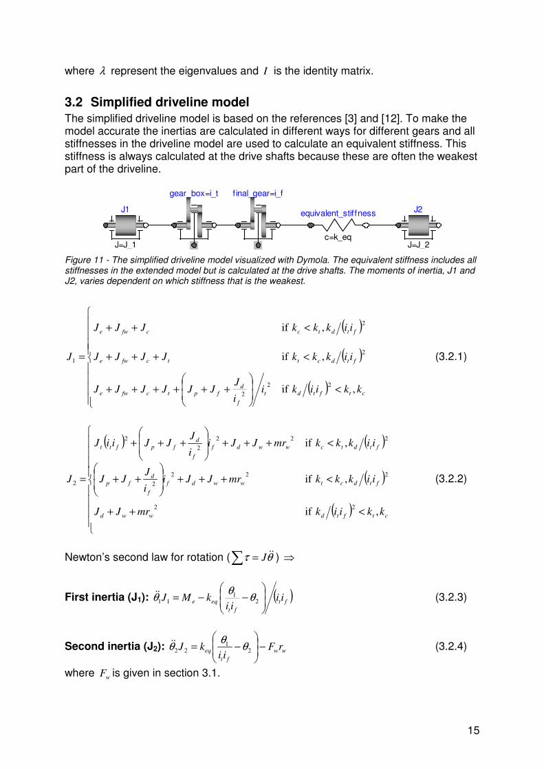
The simplified driveline model is based on the references [3] and [12]. To make the model accurate the inertias are calculated in different ways for different gears and all stiffnesses in the driveline model are used to calculate an equivalent stiffness. This stiffness is always calculated at the drive shafts because these are often the weakest part of the driveline.
J1
J=J_1
J2
J=J_2
equivalent_stiffness
c=k_eq
gear_box=i_t f inal_gear=i_f
Figure 11 - The simplified driveline model visualized with Dymola. The equivalent stiffness includes all stiffnesses in the extended model but is calculated at the drive shafts. The moments of inertia, J1 and J2, varies dependent on which stiffness that is the weakest.
( )
( )
( )
<
++++++
<+++
<++
=
ctftdt
f
dfptcfwe
ftdcttcfwe
ftdtccfwe
kkiikii
JJJJJJJ
iikkkJJJJ
iikkkJJJ
J
, if
, if
, if
22
2
2
2
1 (3.2.1)
( ) ( )
( )
( )
<++
<+++
++
<+++
+++
=
ctftdwwd
ftdctwwdf
f
dfp
ftdtcwwdf
f
dfpftt
kkiikmrJJ
iikkkmrJJii
JJJ
iikkkmrJJii
JJJiiJ
J
, if
, if
, if
22
222
2
222
2
2
2 (3.2.2)
Newton’s second law for rotation (∑ = θτ &&J ) ⇒
First inertia (J1): ( )ft
ft
eqe iiii
kMJ
−−= 2
111 θ
θθ&& (3.2.3)
Second inertia (J2): ww
ft
eq rFii
kJ −
−= 2
122 θ
θθ&& (3.2.4)
where wF is given in section 3.1.

16
3.2.1 State space equations
To analyze this system in a good way it is preferred to describe it on state space form. The drive shaft torsion, the engine speed ( 1θ& ) and the wheel speed ( 2θ& ) are used as state variables (x1, x2 and x3).
=
=
−=
23
12
21
1
θ
θ
θθ
&
&
x
x
iix
ft
(3.2.5)
( )
−=
−=
−=
ww
ft
e
ft
rFkxJ
x
xii
kM
Jx
xii
xx
1
2
3
1
1
2
32
1
1
1
&
&
&
(3.2.6)
On matrix form the state space equations for the simplified driveline model yields
( )( )
( )( )
+−
+
−
+
−
−
−
=
αρ sin
0
0
2
10
0
0
00
110
1
2
3
2
22
1
gcmr
x
rAc
x
A
rmcJk
iiJk
ii
x
rwwaaw
wreq
fteq
ft
444444 8444444 76
&
(3.2.7)
where A is the system matrix.
3.2.2 Natural frequencies
The air drag ( aF ) and the second coefficient of rolling resistance ( 2rc ) have been
neglected when analyzing the frequencies as mentioned in section 3.1.2. The natural frequencies are calculated as in equations (3.1.14) and (3.1.15). For this simplified system, the determinant can be calculated analytically and equation (3.1.15) yields
+±==⇒=
+−⇒
=
−−
−−
2
2
1
3,21
2
2
1
3
2
1
1
)(
1 and 00
)(
0
00/
0)/(
1)/(1
det
JiiJk
J
k
iiJ
k
Jk
iiJk
ii
ft
eq
eq
ft
eq
eq
fteq
ft
λλλλ
λ
λ

17
Equation (3.1.14) then gives the following expression for the natural frequency for the simplified driveline model, using the second or third eigenvalue.
( )
+=
2
2
1
11
2
1
JiiJkf
ft
eqnπ
(3.2.8)

18
4 First weight estimation strategy This strategy is based on frequency analysis of speed data via CAN. If the vehicle’s driveline dynamics are approximated as a spring-mass system with the drive shafts as the weakest link, the equation for the natural frequency would be (analogous with equation (3.2.9)):
+=
2
12
11
2
1
iJJkf eqn
π (4.1.1)
where i is the total gear ratio, keq is the equivalent stiffness of the driveline and 1J
and J2 are the two inertias, respectively. For high gears the ratio ( i) is small making 1
J1i2
>>1
J2
and thus simplifying the expression to
2
1
,2
1
high
eq
highniJ
kf
π= (4.1.2)
where the index “high” indicates that the expression is valid at high gears. An
example that validates this simplification is that, for Ebola 2
2
1
1343
1
JiJ⋅= at the
highest gear and a vehicle weight of 40 000 kg. Every vehicle has its own specific constants like for example the wheel radius, number of cylinders in the engine and stiffness of the drive shafts. These parameters are stored in the different ECU’s control systems in the truck and are used to optimize the vehicle’s performance. Using some of these parameters to calculate the moment of inertia ( 1J ), where the number of included elements depends on the model’s complexity, it is possible to determine the equivalent stiffness of the driveline from equation (4.1.2):
( ) 2
1
2
,2 highhighneq iJfk π= . (4.1.3)
If frequency analysis is applied, the natural frequency ( lown,
ω ) of the driveline can be
determined. In accordance with the reasoning in section 3.1 the truck’s overall mass can be approximated as a rotating point mass with the wheel radius ( rw) as its distance to the centre of rotation. The second moment of inertia ( 2J ) may then be described by
2
2 ww mrJJ += . (4.1.4)
Combining the equations (4.1.1 – 4.1.4) leads to the following expression for the vehicle weight:
19
( )
−
−= w
eqlowlown
loweq
w
JkifJ
iJk
rm
2
,1
2
1
22
1
π.

20
5 Simulation results Simulations are important because they illustrate mathematical relationships that are sometimes hard to see in equations and they are often useful to verify analytic calculations. In this chapter the results from various simulations are presented. First, the results from the two driveline models described in chapter 3 are displayed where the natural frequency of the driveline is shown in relation to different gears and vehicle weights. Second, the models are compared with each other and the analytic results are verified by Dymola simulations. Finally, the results from the simulations are concluded.
The constants that define the driveline’s rotational dynamics have to be accurately known to make a good estimation of the frequency. Appendix 1 and 2 show the constants for Ebola and Mulle, respectively.
5.1 Driveline model
Solving equation (3.1.15) for the state space system described by equation (3.1.13) and using equation (3.1.14) for the second eigenvalue, representing the first oscillation mode of the driveline, gives the results plotted in Figure 12 for Ebola and Figure 13 for Mulle.
CRL1
35
79
11 0.51
1.52
2.53
3.54 x 10
4
0
1
2
3
4
5
6
7
8
X: -1Y: 5000Z: 1.766
Vehicle weight [kg]
Natural frequency of the driveline for the driveline model
X: -1Y: 4e+004Z: 0.8852
X: 12Y: 5000Z: 7.612
Gear
X: 12Y: 4e+004Z: 7.525
Nat
ural
fre
quen
cy f
or t
he d
rivel
ine
[Hz]
Figure 12 - The natural frequency for the driveline model for Ebola. The extreme values of the weight and gear are pinpointed which makes it easy to see that the frequency depend more on the weight for lower gears than for higher.

21
CRL1
35
79
11 0.51
1.52
2.53
3.54 x 10
4
0
1
2
3
4
5
6
7
8
9
X: -1Y: 5000Z: 1.65
Vehicle weight [kg]
Natural frequency for the driveline for the driveline model
X: -1Y: 4e+004Z: 0.8523
X: 12Y: 5000Z: 8.185
Gear
X: 12Y: 4e+004Z: 8.108
Nat
ural
fre
quen
cy f
or t
he d
rivel
ine
[Hz]
Figure 13 - The natural frequency for the driveline model for Mulle.
The labeled corners of the surface point out that the natural frequency depend more on the weight for low gears than for high. This makes it easier to estimate the weight for low gears.
Another conclusion that can be made from studying Figure 12 and Figure 13 is that for higher vehicle weight, the frequency is not as dependent on the weight. Graphically, this means that the slope of the curve along the weight axis gets steeper with decreasing weight and thus making it easier to estimate the weight at low vehicle weight.
5.2 Simplified driveline model
Figure 14 (for Ebola) and Figure 15 (for Mulle) shows the natural frequency for the simplified driveline model, described by equation (3.2.8), for different weights and gears. The constants that have been used for this model are attached in Appendix 1 and 2. The equivalent stiffness has to be calculated for each gear because it depends on the gear ratio and the gearbox stiffness.
( ) ( )
1
222
1111−
+++=
dfpfttftc
eqkikiikiik
k (5.2.1)

22
CRL1
35
79
11 0.51
1.52
2.53
3.54 x 10
4
0
1
2
3
4
5
6
7
8
X: -1Y: 5000Z: 1.765
Vehicle weight [kg]
Natural frequency for the driveline for the simplified driveline model
X: -1Y: 4e+004Z: 0.885
X: 12Y: 5000Z: 7.857
Gear
X: 12Y: 4e+004Z: 7.783
Nat
ural
fre
quen
cy f
or t
he d
rivel
ine
[Hz]
Figure 14 - Natural frequency for the simplified driveline model for Ebola. Once again it is noticeable that the frequency depend more on the weight for low gears than for high gears.

23
CRL1
35
79
11 0.51
1.52
2.53
3.54 x 10
4
0
1
2
3
4
5
6
7
8
X: -1Y: 5000Z: 1.65
Vehicle weight [kg]
Natural frequency for the driveline for the simplified driveline model
X: -1Y: 4e+004Z: 0.8522
X: 12Y: 5000Z: 7.725
Gear
X: 12Y: 4e+004Z: 7.65
Nat
ural
fre
quen
cy f
or t
he d
rivel
ine
[Hz]
Figure 15 - Natural frequency for the simplified driveline model for Mulle.
The corners of the surfaces are labeled to point out that the natural frequency depend more on the weight for low gears than for high gears, which was expected because Figure 12 showed the same property. This property can also be seen in equation (3.2.9) where the gear ratio ( ti ) is high for low gears making the second
inertia ( 2J ) contribute more to the natural frequency (remembering that 2J includes the vehicle weight).
5.3 Comparison between the models
To compare the two driveline models, the natural frequency for the driveline model was subtracted from the natural frequency for the simplified driveline model. The results from this subtraction are displayed in Figure 16 (for Ebola) and Figure 18 (for Mulle).

24
CRL 1 3 5 7 9 110.5
1
1.5
2
2.5
3
3.5
4
x 104
-0.4
-0.3
-0.2
-0.1
0
0.1
0.2
0.3
X: 7Y: 5000Z: -0.01894
Gear
Difference in natural frequency of the driveline betweenthe driveline model and the simplified driveline model
Vehicle weight [kg]
Nat
ural
fre
quen
cy d
iffer
ence
[H
z]
Figure 16 - Comparison between the models for Ebola. The simplified driveline model is a good approximation for gears lower than the seventh.
The difference between the two driveline models is close to zero for gears lower than the seventh for Ebola. For higher gears than the seventh, it is clear that the difference between the models becomes more significant. It is important to remember from section 5.1 that the weight is easier to estimate at lower gears, making the simplified model a reasonable approximation.

25
CRL CRH 1 2 3 4 5 6 7 8 9 10 11 120
2
4
6
8
10
12
14
16
18x 10
4
Gear
Stif
fnes
s [N
m/r
ad]
The stiffnesses which are compared in the simplified driveline model
drive shafts (kd/(i
t2i
f2))
gearbox (kt)
clutch (kc)
Figure 17 - The three stiffnesses, compared in section 3.2 to distribute the inertias, for Ebola. Note that the drive shafts hold the lowest stiffness for all gears except the twelfth, where the clutch is the weakest.
Figure 17 reveals that the drive shafts hold the lowest and hence the dominant stiffness for all gears but the twelfth. At the twelfth gear, the clutch has the lowest stiffness. The inertias are therefore moved, according to section 3.2, so that the value of the first inertia ( 1J ) gets lower and the frequency higher. This explains the appearance of Figure 16 for the highest gear. The reason that the difference between the two models is small for low gears (as seen in Figure 16) is that the drive shaft stiffness is by far the lowest there, making the simplification accurate. For higher gears, the drive shaft stiffness approaches the clutch stiffness, which makes the simplification less accurate. When the drive shaft stiffness is moved, to be able to compare it with the gearbox and the clutch stiffness, it is in inverse proportion to the
quadratic of the gear ratio ( )
2
ft
d
ii
k. The difference displayed in Figure 16 seems to
mirror this behaviour, which strengthens the theory described above.

26
CRL1
35
79
111
2
3
4
x 104
-0.5
-0.45
-0.4
-0.35
-0.3
-0.25
-0.2
-0.15
-0.1
-0.05
0
Vehicle weight [kg]
Difference in natural frequency of the driveline betweenthe driveline model and the simplified driveline model
X: 8Y: 5000Z: -0.02919
Gear
Nat
ural
fre
quen
cy d
iffer
ence
[H
z]
Figure 18 - Comparison between the models for Mulle. The simplified driveline model is a good approximation for gears lower than the eighth.
The difference between the two driveline models is close to zero for gears lower than the eighth for Mulle, making the simplified driveline model a good approximation for those gears.

27
CRL CRH 1 2 3 4 5 6 7 8 9 10 11 120
2
4
6
8
10
12
14
16
18x 10
4
Gear
Stif
fnes
s [N
m/r
ad]
The stiffnesses which are compared in the simplified driveline model
drive shafts (kd/(it2if
2))
gearbox (kt)
clutch (kc)
Figure 19 - The three stiffnesses, compared in section 3.2 to distribute the inertias, for Mulle. The drive shaft stiffness is the lowest for all gears.
In Figure 19 it is obvious that the drive shafts has the lowest stiffness for all gears, which explains why Figure 18 does not show the same behaviour as Figure 16 does for the highest gear.
5.4 Dymola simulations
Dymola is a multi-engineering modelling and simulation tool used in the automotive industry to simulate complex and integrated systems. By the use of Dymola, two models representing the driveline were created and can be viewed in Figure 20 and Figure 21. The idea was to verify that the analytic models were correct and hence secure that the results from these could be trusted. As mentioned earlier in this chapter, the models consist of blocks that represent the driveline’s different parts in terms of stiffness and moment of inertia.
J1
J=J_1
clutch
c=k_c
J2
J=J_2
gear_box
c=k_t
gear__box=i_t
J3
J=J_3
prop_shaft
c=k_p
J4
J=J_4
f inal_gear=i_f
drive_shaft
c=k_d
J5
J=J_5 Figure 20 – Illustration of the Dymola model that represents the rotational dynamics of a truck’s driveline.

28
J1
J=J_1
J2
J=J_2
equivalent_stiffness
c=k_ekv
gear_box=i_t f inal_gear=i_f
Figure 21 – The simplified Dymola model for a truck’s driveline.
Both models were linearized in Dymola and by the use of a MATLAB script written by Eric Gomez at Scania, the natural frequencies were determined through the eigenvalues of the systems. These calculations showed the exact same frequencies as the ones displayed in Figure 12 to Figure 15. Thus, the analytic calculations are correct.
5.5 Simulation conclusions
As stated in section 5.2, the equivalent stiffness varies between different gears because the gear ratio as well as the gearbox stiffness is not constant for different gears. Furthermore, the simplified driveline model does not match the driveline model for high gears. This unfortunately leads to the conclusion that the strategy that has played a central role during the project is not going to work as intended remembering from chapter 4 that the equivalent stiffness ( keq ) has to be the same for both high and
low gears. A new successful strategy would be to analyze the natural frequency of the driveline at low enough engine speed for the engine to excite this frequency (described further in section 6.2.1). In addition, the stiffness of the driveline is determined by the use of constants instead of being calculated from the natural frequency. The resulting frequency could then be used to determine the vehicle weight.

29
6 Frequency analysis It is important to have knowledge about what frequencies to expect when analyzing dynamic systems. This chapter explains how the data that form the basis for the frequency analysis have been selected. In addition, it also gives details on how the natural frequency of the driveline can be determined and how the engine and the propeller shaft contribute to driveline oscillations.
6.1 Data selection
Two methods were used in order to find the frequencies present in the driveline dynamics. The first method includes measuring the vehicle speed with the tachometer described in section 2.5. A typical graph of the vehicle speed during a test drive from Södertälje Technical Centre (STC) to Oxelösund 090129 is displayed in Figure 22.
0 500 1000 1500 2000 2500 3000 3500 40000
10
20
30
40
50
60
70
80
90
Time [s]
Veh
icle
spe
ed [
km/h
]
Vehicle speed from tachometer sensor
Figure 22 – The vehicle speed during a test drive with Mulle between Södertälje Technical Centre and Oxelösund 090129.
Now, if this signal would be used to form the basis for a frequency analysis, the mean value would first have to be removed so that only the frequencies that originate from the vehicle dynamics would appear. This work can become quite extensive and challenging because the speed varies a lot over time and hence making it hard to decide the length of the segment where the mean value should be subtracted.
The second method is based on the ratio between the engine speed (measured with the RPM sensor) and the tachometer speed. The gear ratio, which thereby is formed, oscillates about a gear specific value. The advantage with this method is that the oscillations are preserved at the same time as possible trends are removed. This ratio is plotted in Figure 23 for the test drive STC – Oxelösund 090129. It is clear that

30
this data set is much easier to analyze because the oscillations occur about a specific value (the gear ratio).
0 500 1000 1500 2000 2500 3000 3500 40000
0.5
1
1.5
2
2.5
3
3.5
4
4.5
5
Time [s]
Gea
r ra
tioGear ratio for the gearbox
Figure 23 – The ratio between the input and output shaft speed of the gearbox during the same test drive as displayed in Figure 22.
6.2 Frequency selection
As seen in the figures in chapter 5, the natural frequency of the driveline should approximately lie in the range 1 Hz to 8 Hz, for the test truck Ebola, depending on the gear and the vehicle weight. To measure the natural frequency, there has to be resonance in the driveline. The most likely excitation source is the engine, which oscillates because of the ignition and the forces and moments created when the cylinders move up and down. Another excitation source could be the unbalance in the propeller shaft. To decide with confidence, where the frequencies come from, an oscillation order analysis has been done. This is described in sections 6.2.1 and 6.2.2.
6.2.1 Engine frequency
The cylinders in the engine introduce several frequencies. The highest frequency originates from the motion of each cylinder, i.e. every time a cylinder in the engine changes direction. The lowest frequency comes from the ignition of one single cylinder. The oscillation mode with order one is something that happens once every revolution of the crank shaft. This oscillation mode does not depend on the type of engine, because all truck engines are of four stroke type, but only on the crank shaft speed. The same applies for the oscillation mode of order ½, representing the ignition frequency from one cylinder (a four stroke cylinder ignites every other revolution of the crank shaft), which is the frequency that is most likely to excite the natural frequency of the driveline (see equation (5.1.1)).

31
602
⋅
=n
f ee
ω (5.1.1)
where
cycle per Strokes
[RPM] speed Engine
[Hz] 1/2)(order cylinder one fromfrequency Ignition
=
=
==
n
f
e
e
ω
For a certain engine speed at each gear the engines first oscillation mode may excite the driveline’s natural frequency.
400 600 800 1000 1200 1400 1600 1800 2000 2200 24002
4
6
8
10
12
14
16
18
20
Igni
tion
freq
uenc
y fr
om o
ne c
ylin
der
[Hz]
Engine speed [RPM]
Ignition frequency from one cylinder
Figure 24 - The ignition frequency from one cylinder in a truck engine. The frequency varies between approximately 3.5 Hz and 20 Hz in a normal engine speed range for a truck.
Figure 24 shows that the ignition frequency from the engine is 8 Hz at an engine speed of approximately 1000 RPM. This means that the engine frequency may excite the natural frequency in the driveline at engine speeds of 1000 RPM and lower. The lowest engine frequency possible is approximately 3.5 Hz because of the truck’s idle control system. At gears lower than the sixth, where the natural frequency of the driveline lies beneath 3 Hz, the engine frequency should therefore not excite the natural frequency in the driveline.
An example of the gear ratio Fourier transform is illustrated in Figure 25. In this case it is easy to distinguish between the engine frequency at 10.4 Hz (see Figure 24) and the natural frequency in the driveline at 7.7 Hz.

32
0 5 10 15 20 25 30 35 40 45 500
1
2
x 10-4
X: 10.44Y: 0.0002037
Frequency [Hz]
Am
plitu
de
FFT for the gear ratio at the specified time interval
X: 7.701Y: 0.0001722
X: 1.532Y: 6.301e-005
X: 20.89Y: 7.052e-005
X: 29.07Y: 4.124e-005
X: 39.51Y: 6.41e-005
X: 42.26Y: 2.794e-005
Figure 25 - Fourier transform for the gear ratio for Ebola at the highest gear and ~1200 RPM. The peaks at 10.4 Hz and 7.7 Hz probably correspond to the ignition frequency and the natural frequency for the driveline, respectively.
Because the engine frequencies depend on the engine speed, there should be an engine speed where the ignition frequency oscillates in resonance with driveline, resulting in a high amplitude gain for that specific frequency. To investigate the presence of resonance, the engine speed has been varied for each gear and plotted in 3D-plots. Figure 26 shows that resonance occurs at 3.9 Hz and 487 RPM for the eighth gear for the truck Ebola.

33
010
2030
4050
0
500
1000
1500
2000
2500
0
0.01
0.02
0.03
0.04
0.05
0.06 X: 3.906Y: 487.1Z: 0.05445
Frequency [Hz]
FFT for the gear ratio at gear no. 8 after windowing
Engine speed [RPM]
Am
plitu
de
Figure 26 - The Fourier transform for the gear ratio at varying engine speed for Ebola. Resonance occurs at 487 RPM and 3.9 Hz.
If the first order engine frequency is used to normalize the frequencies from the Fourier analysis, it is easy to decide whether an oscillation comes from the engine or not. The first engine oscillation mode frequency represents something that happens once every crank shaft revolution, i.e. it is the same as engine speed in revolutions per second and can be expressed as
601,
e
efω
= (5.1.2)
where [RPM] speed Engine=eω
The oscillation order with respect to the engine is then calculated as
1,ef
forder =
where [Hz] FFTby frequency Measured=f In Figure 27 an example is shown were the natural frequency is excited by the engine frequency of order 0.5 (the ignition frequency from one cylinder) and a very clear peak at 0.5 is visible. The smaller peaks at 0.4, which are visible for each engine speed, cannot come from the engine because 1/0.4 is no integer. It does not,

34
however, vary with the engine speed so it has to be connected to the speed of the crank shaft in some way. For other gears these smaller peaks occur at other frequencies saying that they must originate from something after the gearbox, for instance the propeller shaft.
00.511.52
0
1000
2000
3000
0
0.01
0.02
0.03
0.04
X: 0.4123Y: 2359Z: 0.0008808
X: 0.5013Y: 479.3Z: 0.0403
FFT for the gear ratio at gear no. 8 after windowing
Oscillation order with respect to the engine
X: 1.083Y: 486.9Z: 0.01103
Engine speed [RPM]
Am
plitu
de
Figure 27 - It is obvious that it is the engine frequency of order 0.5 that excites the driveline. Noticeable are the smaller hills at order 0.4, which cannot come from the engine because 1/0.4 is no integer.
6.2.2 Propeller shaft frequency
The propeller shaft frequency of order one can be expressed as
t
ep
pi
f6060
1,
ωω==
where [RPM] speed shaft Propeller=pω
[RPM] speed Engine=eω
ratio gearGearbox =ti
The oscillation order with respect to the propeller shaft is then calculated as
1,pf
forder =
where [Hz] FFTby frequency Measured=f

35
Figure 28 shows a propeller shaft order plot for the same data as in Figure 27. The small peaks were, as predicted, from the propeller shaft because they all lie at order one.
00.511.522.53
0
1000
2000
3000
0
0.01
0.02
0.03
0.04
0.05
X: 1Y: 1216Z: 0.001658
FFT for the gear ratio at gear no. 8 after windowing
Oscillation order with respect to the propeller shaft
X: 1.219Y: 481.5Z: 0.04936
X: 2.651Y: 486.1Z: 0.01329
Engine speed [RPM]
Am
plitu
de
Figure 28 - The small peaks at oscillation order one represents something that happens once per revolution of the propeller shaft.
It is important to account for where the resonance comes from to know if it really is a resonance and to exclude other frequencies.

36
7 Development of weight estimation method As discussed in section 5.5, the equivalent stiffness of the driveline is not constant for different gears and thus making it difficult to determine the weight using the first strategy. However, if the relation between the stiffness, gear and weight could be approximated by simulations then this information could be used to determine the weight. This concept is investigated further in this chapter.
7.1 Second weight estimation strategy
This method is based on the theory that if a simulation manages to reassemble a real system in an acceptable manner it can be used to calculate certain parameters. By analyzing measured data from the real system and using that information as input to the driveline model simulation, the weight can be estimated. The flow chart of the strategy is showed in Figure 29.
Figure 29 – The flow chart for the second weight estimation method.
0 500 1000 1500 2000 2500 3000 3500 40000
0.5
1
1.5
2
2.5
3
3.5
4
4.5
5
Time [s]
Gea
r ra
tio
Gear ratio for the gearbox
010
2030
4050
0
500
1000
1500
2000
2500
0
0.01
0.02
0.03
0.04
0.05
0.06 X: 3.906Y: 487.1Z: 0.05445
Frequency [Hz]
FFT for the gear ratio at gear no. 8 after windowing
Engine speed [RPM]
Am
plitu
de
CRL1
35
79
110.5
11.5
22.5
33.5
4 x 10⁴
0
1
2
3
4
5
6
7
8
X: -1Y: 5000Z: 1.766
Vehicle weight [kg]
Natural frequency of the driveline for the driveline model
X: -1Y: 4e+004Z: 0.8852
X: 12Y: 5000Z: 7.612
Gear
X: 12Y: 4e+004Z: 7.525
Na
tura
l fr
equ
enc
y fo
r th
e d
rivel
ine
[Hz]
Speed
Gear ratio
Frequency &
Gear
Weight
37
8 Results This chapter presents the results of this thesis. First the results from the frequency analysis are presented, and then the mathematical driveline models are verified followed by the actual weight estimation results.
8.1 Frequency analysis
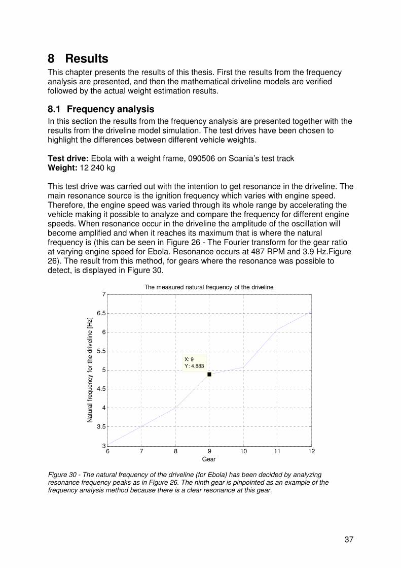
In this section the results from the frequency analysis are presented together with the results from the driveline model simulation. The test drives have been chosen to highlight the differences between different vehicle weights. Test drive: Ebola with a weight frame, 090506 on Scania’s test track Weight: 12 240 kg This test drive was carried out with the intention to get resonance in the driveline. The main resonance source is the ignition frequency which varies with engine speed. Therefore, the engine speed was varied through its whole range by accelerating the vehicle making it possible to analyze and compare the frequency for different engine speeds. When resonance occur in the driveline the amplitude of the oscillation will become amplified and when it reaches its maximum that is where the natural frequency is (this can be seen in Figure 26 - The Fourier transform for the gear ratio at varying engine speed for Ebola. Resonance occurs at 487 RPM and 3.9 Hz.Figure 26). The result from this method, for gears where the resonance was possible to detect, is displayed in Figure 30.
6 7 8 9 10 11 123
3.5
4
4.5
5
5.5
6
6.5
7
X: 9Y: 4.883
Nat
ural
fre
quen
cy f
or t
he d
rivel
ine
[Hz]
Gear
The measured natural frequency of the driveline
Figure 30 - The natural frequency of the driveline (for Ebola) has been decided by analyzing resonance frequency peaks as in Figure 26. The ninth gear is pinpointed as an example of the frequency analysis method because there is a clear resonance at this gear.

38
6 7 8 9 10 11 122.5
3
3.5
4
4.5
5
5.5
6
6.5
7
7.5
8
X: 9Y: 4.919
Gear
Nat
ural
fre
quen
cy o
f th
e dr
ivel
ine
[Hz]
The natural frequency of the driveline at thevehicle weight 12240 kg for the driveline model
Figure 31 - The natural frequency of the driveline described in section 3.1 for Ebola. By comparing this plot with Figure 30 it is clear that they do not match exactly. They match relatively well at the lower gears where the weight affects the frequency the most.
At the ninth gear there is a clear resonance in the gear ratio signal. Therefore, this gear is pinpointed in Figure 30 and Figure 31. This resonance is shown in Figure 32 and Figure 33 and occurs at low engine speeds where the engine frequency excites the natural frequency of the driveline.
05
1015
2025
500
1000
1500
2000
2500
0
0.005
0.01
0.015
0.02
Frequency [Hz] (X)
FFT for the gear ratio at gear no. 9 after windowing
X: 4.883Y: 478.3Z: 0.01321
Engine speed [RPM] (Y)
Am
plitu
de [
-] Z
Figure 32 - Fourier transform of the gear ratio during a test drive with Ebola. At 4.883 Hz, the engine frequency excites the natural frequency at 478.3 rpm.

39
1600 1650 1700 1750 1800
1.8
1.85
1.9
1.95
2
2.05
2.1
Time [s]
Gea
r ra
tio [
-]
Gear ratio for the gearbox
Figure 33 – The calculated gear ratio at the ninth gear where the resonance in the driveline is obvious. This is why the frequency shown in Figure 32 is so easy to spot.
Test drive: Ebola with a trailer, 090506 on Scania’s test track Weight: 36 320 kg The test method was the same as the one described above. When driving in uphill slopes at low gears and low engine speed, the engine torque was so high that the wheels slipped. At plane ground, the engine’s idle control made it impossible to achieve resonance (described in section 6.2.1) for lower gears than the seventh. Comparing Figure 34 and Figure 35 it is obvious that the model does not fit the measured data well, other than for gear seven. These results are still important because the weight estimation method is better for lower gears (as explained in section 5.1).

40
7 8 9 10 11 123
3.5
4
4.5
5
5.5
6
6.5
Nat
ural
fre
quen
cy f
or t
he d
rivel
ine
[Hz]
Gear
The measured natural frequency of the driveline
Figure 34 - The measured frequency should be a little lower for this test drive than for the one described above because of the higher vehicle weight, which it is.
7 8 9 10 11 123
3.5
4
4.5
5
5.5
6
6.5
7
7.5
8
Gear
Nat
ural
fre
quen
cy f
or t
he d
rivel
ine
[Hz]
The natural frequency of the driveline at thevehicle weight 36320 kg for the driveline model
Figure 35 - The natural frequency from the driveline model described in section 3.1 for Ebola. Comparing this figure with Figure 34 it is clear that only the seventh gear match the measured data well.

41
Test drive: Mulle, 090525 on Scania’s test track Weight: 12 590 kg This test was performed in the same manner as the tests described previously in this section.
4 5 6 7 8 9 10 11 121
1.5
2
2.5
3
3.5
4
4.5
5
5.5
6
6.5
7
Nat
ural
fre
quen
cy f
or t
he d
rivel
ine
[Hz]
Gear
The measured natural frequency of the driveline
Figure 36 - The measured frequency for Mulle. The reason why the frequency is the same for the eighth and the ninth gear is explained later in this section.
4 5 6 7 8 9 10 11 122
2.5
3
3.5
4
4.5
5
5.5
6
6.5
7
7.5
8
8.5
9
Gear
Nat
ural
fre
quen
cy f
or t
he d
rivel
ine
[Hz]
The natural frequency of the driveline at thevehicle weight 12590 kg for the driveline model
Figure 37 - The natural frequency of the driveline described in section 3.1 for Mulle.

42
It is obvious that the model fits the measured data better at low gears than at high, just as for Ebola. The best matches are found at the fourth, seventh and eighth gear. The resonance should occur at lower engine speeds for lower gears. However, for this test drive the resonance for the eighth gear occurs at a higher engine speed than for the ninth, which can be seen in Figure 38 and Figure 39. This means that the true natural frequency of the driveline at the eighth gear is probably lower than the measured and could not be seen because the engine speed was not low enough. The resonance at the eighth gear must then be due to the engine frequency being close to the natural frequency and not exactly the same.
0510152025
500
1000
1500
2000
0
0.005
0.01
0.015
0.02
0.025 X: 4.004Y: 508.9Z: 0.02067
FFT for the gear ratio at gear no. 9 after windowing
Frequency [Hz] (X)
Engine speed [RPM] (Y)
Am
plitu
de [
-] (
Z)
Figure 38 - The Fourier transform for Mulle at the ninth gear and varying engine speed. Noticeable is that there are a number of resonance peaks around the natural frequency of the driveline.

43
0510152025
500
1000
1500
2000
0
0.005
0.01
0.015
0.02
X: 4.004Y: 515.7Z: 0.01836
FFT for the gear ratio at gear no. 8 after windowing
Frequency [Hz] (X)Engine speed [RPM] (Y)
Am
plitu
de [
-] (
Z)
Figure 39 - The Fourier transform for Mulle at the eighth gear and varying engine speed. The resonance peak at 4.004 Hz could be a frequency close to the natural frequency of the driveline, which has been amplified as in Figure 38.
An example of the phenomenon that the resonance peak is spread over several different engine speeds is shown in Figure 40. This is why it is so difficult to determine if a peak is the actual natural frequency.
0
5
10
15
20
25
400600
8001000
12001400
0
0.005
0.01
0.015
0.02
Frequency [Hz] (X)
FFT for the gear ratio at gear no. 11 after windowing
X: 5.762Y: 709.3Z: 0.0165
Engine speed [RPM] (Y)
Am
plitu
de [
-] (
Z)
Figure 40 - The Fourier transform for Mulle at the eleventh gear and varying engine speed. It is clear that there is resonance at several different engine speeds, but the peak is higher for the pinpointed speed indicating that this must be the natural frequency of the driveline.

44
Test drive: Mulle, 090121 Södertälje to Nyköping Weight: 12 590 kg
At this test drive it is difficult to see resonance peaks at any gear. Most data is collected for the twelfth gear because the test was carried out mostly on a motorway. Although there is a lot of data for this gear, as seen in Figure 41, there is no resonance because of the high engine speed when driving on the motorway.
05
1015
2025
900
1000
1100
1200
0
0.5
1
1.5
x 10-3
X: 7.324Y: 1151Z: 0.0007747
Frequency [Hz] (X)
X: 5.957Y: 949.4Z: 0.0007775
FFT for the gear ratio at gear no. 12 after windowing
Engine speed [RPM] (Y)
Am
plitu
de [
-] (
Z)
Figure 41 - Fourier transform of the gear ratio for the test drive from Södertälje to Nyköping with Mulle. There is no sign of any resonance in the driveline. The only visible frequencies are the ones that originate from the ignition, which are pinpointed at two different engine speeds.
8.2 Model verification
Comparing the measured frequencies (for example Figure 30) and the modelled frequencies (for example Figure 31) it is easy to see that the driveline model described in section 3.1 gives a good estimate of the natural frequency of the driveline for low gears, but not for high. The simplified model (Figure 42 and Figure 43) does not give as good results as the driveline model for low gears, where the most accurate weight estimation is possible, and has therefore not been used for weight estimation.

45
6 7 8 9 10 11 122
2.5
3
3.5
4
4.5
5
5.5
6
6.5
7
7.5
8
Gear
Nat
ural
fre
quen
cy f
or t
he d
rivel
ine
[Hz]
The natural frequency of the driveline at the vehicleweight 12240 kg for the simplified driveline model
Figure 42 - The simulation results from the simplified driveline model for Ebola with a weight of 12 240 kg. This model does not match the Fourier transform results in Figure 30 for low gears and has therefore not been used when estimating the weight.
4 5 6 7 8 9 10 11 122
2.5
3
3.5
4
4.5
5
5.5
6
6.5
7
7.5
8
Gear
Nat
ural
fre
quen
cy f
or t
he d
rivel
ine
[Hz]
The natural frequency of the driveline at the vehicleweight 12590 kg for the simplified driveline model
Figure 43 - The simulation results from the simplified driveline model for Mulle with a weight of 12 590 kg. This model does not match the Fourier transform results in Figure 36 for low gears and has therefore not been used when estimating the weight.
It is difficult to see any resonance peaks for low gears and for high gears, the frequencies from the driveline model and the measured data does not match well.

46
This means that the weight should be estimated at the lowest gear where the resonance frequency is detectable.
8.3 Weight estimation
As described in chapter 6 the weight is estimated by using the driveline model described in section 3.1. Doing so, the weight can be estimated without solving the complex driveline equations analytically. This section presents the results of this weight estimation method. Test drive: Ebola, 090506 on Scania’s test track Weight: 12 240 kg As an example of this weight estimation method, the frequency as a function of the vehicle weight at the ninth gear is given in Figure 44. The measured frequency (see Figure 30) is pinpointed in Figure 44 and corresponds to the estimated weight 20 580 kg.
1 1.2 1.4 1.6 1.8 2 2.2 2.4 2.6 2.8 3
x 104
4.86
4.87
4.88
4.89
4.9
4.91
4.92
4.93
4.94
X: 2.058e+004Y: 4.883
Vehicle weight [kg]
Nat
ural
fre
quen
cy f
or t
he d
rivel
ine
[Hz]
The natural frequency of the driveline at the 9:th gear for the driveline model
Figure 44 - The natural frequency of the driveline as function of the vehicle weight at the ninth gear for Ebola.
The same principle has been applied to all gears where it is possible to see any resonance peaks (gears 6 to 12) and the result is presented in Figure 45.

47
6 7 8 9 10 11 120
10
20
30
40
50
60
Est
imat
ed w
eigh
t [t
onne
s]
Gear
The weight estimation
Estimated weight
Actual weight, m = 12240 kg
Figure 45 - The weight estimation for different gears for the truck Ebola with a weight frame. The weight estimation gives best result at the sixth and the seventh gear and poor result for other gears. The estimations over 65 tonnes have been excluded.
The weight estimation from the test drive 090506 on Scania’s test track with the truck Ebola is showed in Figure 45. Noticeable is that the weight estimate is quite good for low gears (gear number 6 and 7) but inaccurate at higher gears. There are two likely factors explaining this. The first one being that the driveline model is more correct at low gears, as discussed in section 8.2. The second factor has to do with the relation between the natural frequency and the vehicle weight, as explained in section 5.1, making it difficult to estimate the weight at high gears.

48
Test drive: Ebola with a trailer, 090506 on Scania’s test track Weight: 36 320 kg
7 8 9 10 11 120
10
20
30
40
50
60E
stim
ated
wei
ght
[ton
nes]
Gear
The weight estimation
Estimated weight
Actual weight, m = 36320 kg
Figure 46 - The estimated weight for Ebola with a trailer connected. The weight estimation method does not work well because of the low accuracy in the frequency selection.
Figure 46, which shows a test drive for Ebola with a trailer, reveals that the weight estimation method does not work well for higher vehicle weight as predicted in simulations (section 5.1).

49
Test drive: Mulle, 090525 on Scania’s test track Weight: 12 590 kg The final test drive was done with Mulle on Scania’s test track and the weight estimation is illustrated in Figure 47.
4 5 6 7 8 9 10 11 120
10
20
30
40
50
60
Est
imat
ed w
eigh
t [t
onne
s]
Gear
The weight estimation
Estimated weight
Actual weight, m = 12590 kg
Figure 47 - The estimated weight for Mulle is not accurate for any gear. This is probably due to the uncertainty in the constant values of the stiffnesses and moments of inertia in the driveline model.
It is obvious that this estimation is not as good as the one for Ebola. One of the reasons for this may be the uncertainties related to the constants used in the driveline model. Another cause could be the fact that Mulle has an eight cylinder engine, which probably runs in a smoother manner than Ebola’s six cylinder engine. The smoother an engine runs, the more difficult it is to excite the natural frequency of the driveline.

50
9 Analysis and discussion The natural frequency of the driveline varies less with the vehicle weight for higher gears, making it harder to estimate the weight for those gears. On the other hand, it is a problem to estimate the frequency for low gears since the engine speed has to be very low for the engine frequency to excite the natural frequency of the driveline. For this reason, the lowest gear where resonance occurs should give the best weight estimation.
It is difficult to distinguish the propeller shaft frequency from the natural frequency of the driveline because the propeller shaft does not seem to excite the driveline and both frequencies depend on the gear ratio in a similar way. Also, to get a good weight estimation, the constant values of the moments of inertia and the stiffnesses have to be accurately decided for each gear. Difficulties arise because the values of these constants are probably not accurate enough to get a good estimation. The reason for this is that the natural frequency varies so little with the vehicle weight at higher gears where resonance could occur and thereby making an estimation possible.
It is important to know that a lot of effort is done trying to avoid or when necessary damp oscillations in the driveline. This has much to do with the driver comfort in the cab as well as wear and tear of the vehicle. At present there are two main ways of doing this. The first technique is to use a clutch that is designed specifically for the engine used in the truck. By selecting the stiffness of the clutch in a smart way it is possible to determine in what engine speed range the resonance in the driveline will occur and hence choose an engine range that is seldom used. The other technique is to use active gear shifting control. Most trucks now have electronic controlled gear shifting, which makes it possible to avoid engine speeds that produce resonance. In conclusion, resonance wants to be avoided, which will make it difficult to use the strategies discussed in this thesis.
9.1 Uncertainties
As stated in this chapter’s introduction, the values that define the driveline models are related to some uncertainty. That is, both the components moment of inertia and their related stiffness are difficult determine with great accuracy. Every driveline is a bit different when it comes to moments of inertia, stiffness and the natural frequency linked to these. This is mainly due to that there are so many connections between all the mechanical elements that the complex driveline consists of. It would be very difficult trying to take every driveline component into account when building a model. There are always simplifications that have to be made (in order to make the model executable) and hence introducing small errors.
The sensor resolution should not be a big source of uncertainty because the frequencies of interest are in the range of up to about 20 Hz. Also, the CAN protocol should not conflict with the resolution from the sensors because the CAN bus that transmits the speed data is not that strained so the send frequency is affected.
9.2 Comparison with existing methods
Mainly due to the difficulties of determining the natural frequency of the driveline the estimation method does not work as intended and is not better than existing methods. During circumstances where it has been possible to detect this frequency the estimated weight has not been very accurate. The existing methods are not

51
precise either but they do, in contrast with the method investigated, have an error which lies within certain limits.

52
10 Conclusions To conclude the results of this thesis, the investigated weight estimation method is not better than the existing methods. The engine frequency of order ½, described in section 6.2.1, is crucial for the method because that is the frequency which excites the natural frequency of the driveline, creating resonance. The engine frequency depends on the engine speed and the clutch of a vehicle is chosen to avoid resonance at the more commonly used engine speeds. That is the main reason why the resonance frequencies are difficult to see and why this weight estimation method does not work as good as the existing ones.
To estimate the weight, low gears are preferred because the weight estimate is not as dependent on the accuracy of the frequency selection there. However, the natural frequency of the driveline is lower for lower gears. This means that in order to get resonance, originating from the engine ignition, the required engine speed has to be very low. This is difficult to achieve, especially for the lowest gears, where the required speed is lower than the idle speed. This tradeoff between high and low gears is another difficulty with this weight estimation method.

53
11 Future work As mentioned in the previous chapter, this method is no good alternative for estimating the weight of a truck. Therefore, the recommendation to Scania is to not investigate the method further until the natural frequency of the driveline can be decided with greater accuracy. However, the theory from this thesis work could be of interest for other areas than weight estimation. For instance, the driveline stiffness could be approximated by estimating the resonance frequency. By monitoring the driveline stiffness, several applications would be possible.

54
References
[1] Andersson, Lennart et al. 1999 Linjär algebra med geometri, Studentlitteratur, Lund, Sweden
[2] Andersson, Per 2007 Beräkning av tröghetsmoment på ingående axel för
GRS905, Report at Scania CV AB [3] Bruce, Maria 2005 Model Based Powertrain Control, Damping of Oscillations
in a Heavy Duty Vehicle, Thesis for the degree of licentiate engineering, Department of signals and systems, Chalmers University of Technology, Sweden
[4] Dahlberg, Tore 2001 Teknisk hållfasthet, tredje upplagan, Studentlitteratur,
Lund, Sweden [5] Dawoud, Ghena 2005 Vridstyvhet av växellådan GRS905, Report at Scania
CV AB [6] Glad, Torkel & Ljung, Lennart 2006 Reglerteknik, grundläggande teori, fjärde
upplagan, Studentlitteratur, Lund, Sweden
[7] Glad, Torkel & Ljung, Lennart 1997 Reglerteknik, flervariabla och olinjära metoder, Studentlitteratur, Lund, Sweden
[8] Gomez, Erik 2008 Parameterstudie av Egensvägningar I Drivlinan Vid Lågt
Motorvarvtal, Internal report at Scania CV AB [9] Gomez, Erik 2008 Low-Rev Opticruise: Mätdata av Drivlinesvängningar på
Provbilen Moby och Linné, Internal report at Scania CV AB
[10] Gustafsson, Fredrik & Ljung, Lennart & Millnert, Mille 2001 Signalbehandling, Studentlitteratur, Lund, Sweden
[11] Jansson, Per-Johan 2005 Driveline modelling for different vehicle
combination for simulation in Adams, Internal report at Scania CV AB
[12] Petterson, Magnus 1997 Driveline modeling and control, Linköpings tryckeri AB, Sweden
[13] Pytel, Andrew & Kiusalaas, Jaan 2001 Engineering Mechanics: Dynamics,
second edition Thomson Learning, United Kingdom [14] Ritzén, Emil 1997 Adaptive vehicle weight estimation, Master thesis at
Linköping Institute of Technology, Department of Electrical Engineering, Sweden
[15] Schubert, Olle & Örning, Camilla 2008 Vikter och trögheter på komponenter I
vevrörelsen, Internal report at Scania CV AB
55
[16] Skött, Mats 1993 Kardanaxel och Mellanaxel P300, P400, P500, P600 Produktionsutförande -91, -92 Vridstyvhet och Statisk Hållfasthet, Report at Scania CV AB
[17] Wong, J. Y. 2001 Theory of ground vehicles, third edition, John Wiley &
Sons, Inc., Canada

56
Appendix 1 – Ebola constants These constants have been excluded due to Scania’s secrecy policy.

57
Appendix 2 – Mulle constants These constants have been excluded due to Scania’s secrecy policy.

58
Appendix 3 – Drive shaft stiffness and inertia The drive shafts are assumed to be homogenous cylinders with dimensions and material according to the drawing for the current drive shafts. All calculations are for one drive shaft and the stiffness and inertia has to be multiplied by two to fit the drive shaft models described in this thesis. Stiffness According to [4] the torsion angle (θ ) of a straight, homogenous shaft is given by
v
v
GK
LM=θ (1)
where vM is the torque in the shaft
L is the length of the shaft G is the shear modulus vK is the torsion constant
For a homogenous circular shaft the torsion constant is
32
4D
K v
π= (2)
where D is the diameter of the shaft. The shear modulus is calculated from Young’s modulus ( E ) and Poisson’s ratio (ν ).
( )ν+=
12
EG (3)
The torsional stiffness is defined as the fraction between torque and torsion angle
=
θvM
k . The definition of torsional stiffness together with equations (1), (2) and (3)
gives the expression for the stiffness for one drive shaft.
( )ν
π
+=
164
4
L
EDkd

59
Moment of inertia The moment of inertia for a circular, homogenous shaft is given by
8
2mD
J = (4)
The mass ( m ) for a drive shaft is given by the density ( ρ ) and the volume (V ) of the shaft.
Vm ρ= (5) The volume for a circular homogenous shaft is
4
4 LDV
π=
Using the constants stated in the stiffness calculations, the moment of inertia for each drive shaft can be determined.
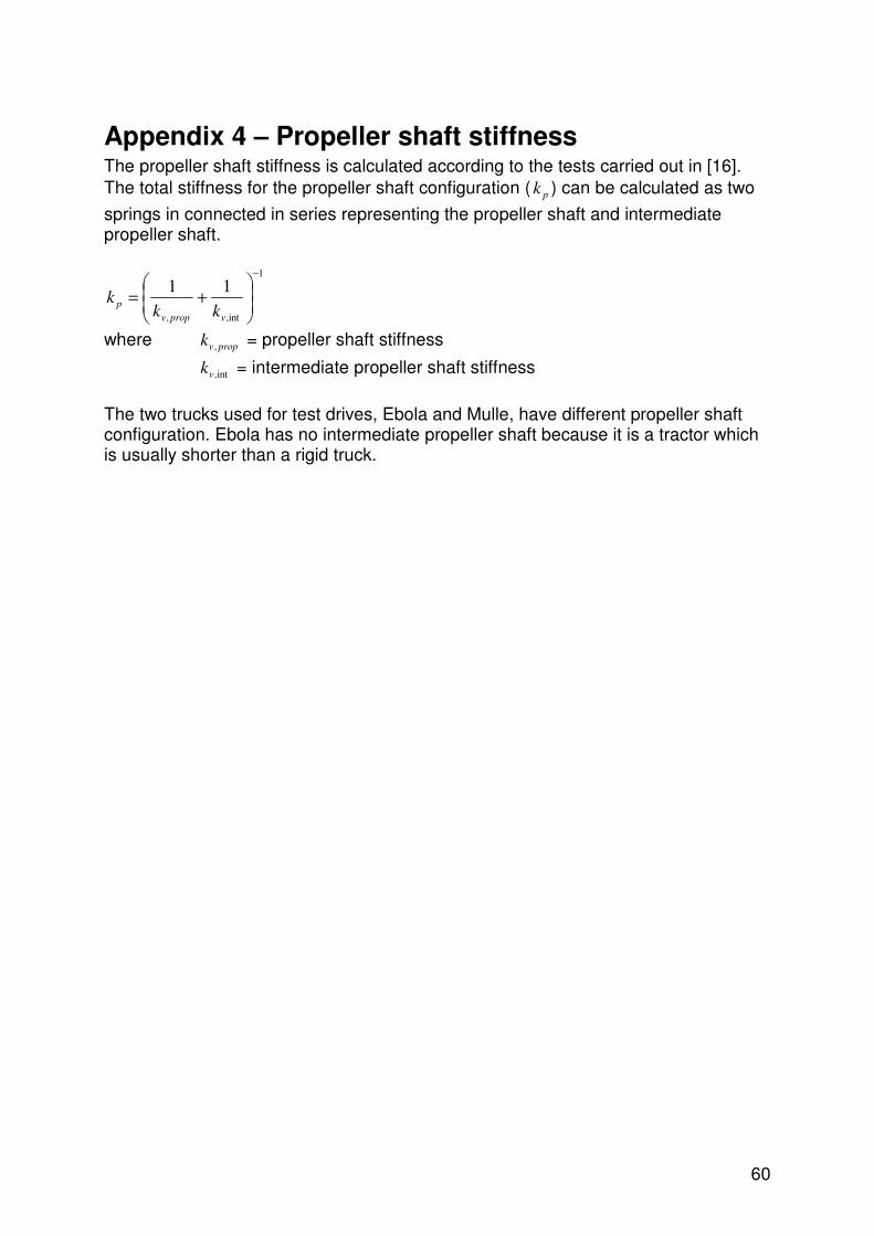
60
Appendix 4 – Propeller shaft stiffness The propeller shaft stiffness is calculated according to the tests carried out in [16]. The total stiffness for the propeller shaft configuration ( pk ) can be calculated as two
springs in connected in series representing the propeller shaft and intermediate propeller shaft.
1
int,,
11−
+=
vpropv
pkk
k
where propvk , = propeller shaft stiffness
,intvk = intermediate propeller shaft stiffness
The two trucks used for test drives, Ebola and Mulle, have different propeller shaft configuration. Ebola has no intermediate propeller shaft because it is a tractor which is usually shorter than a rigid truck.