week 3: supervised learning today's lectures - the semantica...

1/29/16 lecture3_1

file:///home/dt07dm0/EDA025F/EDA025F/lectures/lecture3/lecture3.html 1/74

Week 3: Supervised learning### Today's lecturer: Dennis Medved

Today's lecturesOverview of machinelearning algorithms. Some linear algebra. How to design a ML pipeline.Programming with MLlib.

Today's scheduleOverview of machine learning and linear algebra. <Exercise in linear algebra.Regression and machine learning (ML) pipeline.Exercise in linear regression.Classification and logistic regression.Exercise in logistic regression.

Overview of machinelearning

A definition:### Machine learning is related to statistics.### Cultures and backgrounds are different.### More specifically, explores the construction and study of algorithms that can:

### Learn from data and### Make predictions on data.

1/29/16 lecture3_1


Examples of machinelearningSpam filtering

1/29/16 lecture3_1


Examples of machinelearning (continued)Optical character recognition (OCR)

1/29/16 lecture3_1


Examples of machinelearning (continued)Protein structure prediction

1/29/16 lecture3_1


Examples of machinelearning (continued)Playing Jeopardy

1/29/16 lecture3_1


Examples of machinelearning (continued)Machine vision

Vocabulary

Observations Examples used for learning or evaluation, e.g. wikipedia articles, scanned characters, and films.

Feature A feature is an individual measurable property of an observation, represented as a number or category,e.g. length, year, director.

Label The category or value attached to an observation, e.g. cancer or not cancer, shoe size, score.

1/29/16 lecture3_1


Data set exampleData from Internet Movie DataBase (IMDB)

Title year length director score

The Shawshank Redemption 1994 142 Frank Darabont 9.3

The Godfather 1972 175 Francis Ford Coppola 9.2

Saving Christmas 2014 80 Darren Doane 1.6

Disaster Movie 2008 87 Jason Friedberg 1.9

Models and performance

Model A function that takes the feature vector as input and produces an output, which predicts the category ora value, e.g. a model produced by logistic regression.

Title year length director score




Disaster Movie 2008 87 Jason Friedberg 1.9

Pulp Fiction 1994 154 Quentin Tarantino ? <model

Performance MeasureA measure of of the quality of the predicted label compared to the real label of the observations, e.g.mean absolute value or accuracy. In our case the score (label) is 8.9, the closer, the better.

1/29/16 lecture3_1


Performance evaluation framework

Training, validation, and test data The data set consists of observations (together with their labels) used in training and evaluating themodel, e.g. a set of potential cancer patients.

The data set is usually split up in the three following subsets:

Training data is used to train the model.Validation data is used to improve the performance of the model, by evaluating the result andchanging the model accordingly.Test data is used to evaluate the end result, do not use this for model selection.

The distribution is for example: 70% / 15% / 15%.

Cross validationThe whole data set is partitioned into k equal sized subsamples.

Of the k subsamples, a single subsample (in red) is retained as the validation data for testing themodel, and the remaining k − 1 samples are used as training data.

The crossvalidation process is then repeated k times (the folds). A normal value for k is 5.

1/29/16 lecture3_1


Broad learning settings

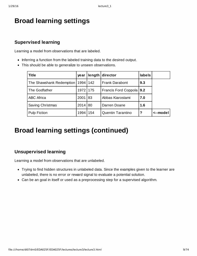
Supervised learning

Learning a model from observations that are labeled.

Inferring a function from the labeled training data to the desired output.This should be able to generalize to unseen observations.

Title year length director labels



ABC Africa 2001 83 Abbas Kiarostami 7.0


Pulp Fiction 1994 154 Quentin Tarantino ? <model

Broad learning settings (continued)

Unsupervised learning

Learning a model from observations that are unlabeled.

Trying to find hidden structures in unlabeled data. Since the examples given to the learner areunlabeled, there is no error or reward signal to evaluate a potential solution.Can be an goal in itself or used as a preprocessing step for a supervised algorithm.

1/29/16 lecture3_1


Supervised learning

Regression

Outputs a real value from an observation, e.g. the IMDB score.

The output is continous (the score, a real number).Evaluation defined by the closeness on the real values.

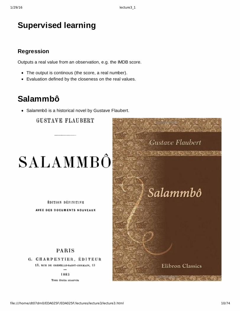
SalammbôSalammbô is a historical novel by Gustave Flaubert.

1/29/16 lecture3_1


Salammbô (continued)Original in French, but there exists an English translation.

Chapter French # chars # A English # chars # A

1 36,961 2,503 35,680 2,217

2 43,621 2,992 42,514 2,761

3 15,694 1,042 15,162 990

4 36,231 2,487 35,298 2,274

5 29,945 2,014 29,800 1,865

6 40,588 2,805 40,255 2,606

7 75,255 5,062 74,532 4,805

8 37,709 2,643 37,464 2,396

9 30,899 2,126 31,030 1,993

10 25,486 1,784 24,843 1,627

11 37,497 2,641 36,172 2,375

12 40,398 2,766 39,552 2,560

13 74,105 5,047 72,545 4,597

14 76,725 5,312 75,352 4,871

15 18,317 1,215 18,031 1,119

1/29/16 lecture3_1


Example of regressionRegression on French version: given the number of characters, predict the number of A:s

# chars on xaxis# A on Yaxis:

1/29/16 lecture3_1


Supervised learning (continued)

Classification

Outputs a class or category for each observation, e.g:

French orEnglish

depending on the number of characters and A:s.

The output is discrete.Closeness can not usually be defined on categories.

Example of classificationClassifying the language in Salammbô: French is the green line, English the purple:

1/29/16 lecture3_1


Here the classifier is a straight line.

1/29/16 lecture3_1


Example of classification (continued)Binary classification, class: 1 = French, 0 = English:

Chapter French # chars # A Class English # chars # A Class

1 36,961 2,503 1 35,680 2,217 0

2 43,621 2,992 1 42,514 2,761 0

3 15,694 1,042 1 15,162 990 0

4 36,231 2,487 1 35,298 2,274 0

5 29,945 2,014 1 29,800 1,865 0

6 40,588 2,805 1 40,255 2,606 0

7 75,255 5,062 1 74,532 4,805 0

8 37,709 2,643 1 37,464 2,396 0

9 30,899 2,126 1 31,030 1,993 0

10 25,486 1,784 1 24,843 1,627 0

11 37,497 2,641 1 36,172 2,375 0

12 40,398 2,766 1 39,552 2,560 0

13 74,105 5,047 1 72,545 4,597 0

14 76,725 5,312 1 75,352 4,871 0

15 18,317 1,215 1 18,031 1,119 0

Unsupervised learning

Dimensionality reduction

The task to transforms the data in a higher dimensional space to a space of fewer dimensionsEnables us to visualize the data in 2D.

1/29/16 lecture3_1


Example of dimensionality reduction77 dimensions reduced to 2Blue points are patients that are alive, red are deadTrue version on the left, predicted on the right:

Unsupervised learning (continued)

Clustering

The task to group observations in clustersThe observations in a cluster are more "similar" to each other than to those in other clustersE.g. clustering different customer types together.

1/29/16 lecture3_1


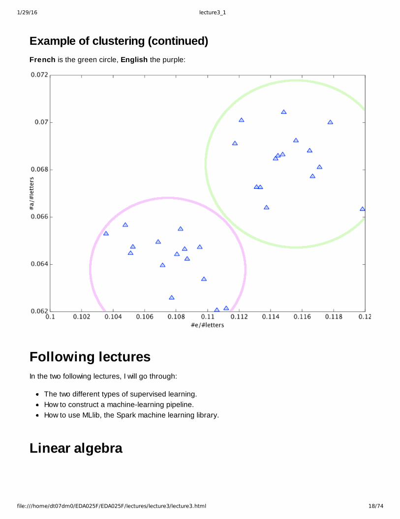
Example of clusteringClustering of Salammbô: Relative frequency:

E:s on XaxisA:s on Yaxis

1/29/16 lecture3_1


Example of clustering (continued)French is the green circle, English the purple:

Following lecturesIn the two following lectures, I will go through:

The two different types of supervised learning.How to construct a machinelearning pipeline.How to use MLlib, the Spark machine learning library.

Linear algebra

1/29/16 lecture3_1


MatricesWe represent data sets using matrices.

A matrix is a rectangular array of numbers, where in our case:

The rows are the observations, in the example below the movies Shawshank Redemption andthe Godfather.The columns are the features: year, length, number of Oscars, first weekend box office.

A =1994 142 7 7273271972 175 3 302393

Matrices are symbolized using bold uppercase letters, e.g. A in the example above.An n × m matrix has n rows and m columns, e.g. A is 2 × 5 matrix.

Matrices (continued)

A =1994 142 7 7273271972 175 3 302393 A =

a1 ,1 a1 ,2 a1 ,3 a1 ,4a2 ,1 a2 ,2 a2 ,3 a2 ,4

Entries are denoted using lowercase letter with two subscript indices, ai , j corresponds to theentry at the ith row and jth column, e.g. a2 , 4 = 302393.

VectorsA vector is a special case of a matrix with several rows and one column or one row and severalcolumns. It is a 1 dimensional data structure (here representing class and scores).

w =10 v =

9.39.2 v =

a1a2

Vectors are denoted by bold lowercase letters, e.g. v in the example above.Entries are symbolized by lowercase letters with one subscript index. For instance, aicorresponds to the entry at the ith row.

[ ]

[ ] [ ]

[ ] [ ] [ ]

1/29/16 lecture3_1


NumPyNumPy is the standard Python library to perform numerical computing. It adds:

Multidimensional arrays and matrices, to store the data sets.A large library of highlevel mathematical functions to operate on these arrays.It is used by MLlib.

In [14]:

# The convention is to import NumPy as the alias npimport numpy as np

Creating arrays with NumPyNumpy's array class is called ndarray; it is also known by the alias array.Ndarray is a multidimensional array of fixedsize that contains numerical elements of one type,e.g. floats or integers.Creating an array from a python list of numbers results into a onedimensional array, which is,for our purposes, equivalent to a vector.You can also use the following class to represent matrices: np.matrix().

Ndarray exampleTo create a matrix object, either pass the constructor a twodimensional ndarray, or a list oflists to the function, or a string e.g. '1 2; 3 4'.

A =1994 142 7 7273271972 175 3 302393 v =

10

Utilizing the np.array() to create the above matrix and vector:

[ ] [ ]

1/29/16 lecture3_1


In [15]:

A = np.array([[1994,142,7,7273274], [ 1972,175,3,302393 ]])v = np.array([1,0])

print(str(A)) print(str(v))

[[ 1994 142 7 7273274] [ 1972 175 3 302393]][1 0]

NormNorm defines the length or magnitude of a vector.In many cases we need to know the magnitude of the observations.In the IMDB data set, a succesful movie will have greater magnitude.Pnorms are usually used.

Mv Mp = (n

∑i=1

| xi |p)1 /p

The pnorm of a vector v is denoted by MvMp.

Euclidian normThe Euclidian norm is the special case of the pnorm when p = 2.Capture the intuitive notion of length of a vector.

Mv Mp = (n

∑i=1

| xi |p)1 / p ã M v M2 =

n

∑i=1

xi2 = x1

2 + ø + xn2

Norm exampleA = 1994 142 7 727327 M v M2 = √19942 + 1422 + 72 + 7273272 ≈ 7273274

NumPy has built in function to calculate the Euclidian norm of a vector, np.linalg.norm(v):

√ √

[ ]

1/29/16 lecture3_1


In [16]:

v = A[0] #[1994,142,7,7273274]norm = np.linalg.norm(v)print(norm)

7273274.27472

Infinity normThe infinity norm is the special case of the pnorm when p = ∞.

MvM∞ = max ( xi )

Property of the norms pnorms: MvM∞ ≤ MvM2

NormalizingIn the IMDB data set, the box office feature outweighs the number of Oscars for example.

A =1994 142 7 7273271972 175 3 302393

The idea is to normalize the features so they become more homogeneous.This usually improves the prediction result and speeds up the training of the model.

Normalizing (continued)Normalizing a feature vector, i.e. making the feature vector have unit length, i.e. length = 1 inthe norm:

Mv Mp = (n

∑i=1

| xi |p)1 /p v ′ =

vMvMp

M v ′ M = 1

Normalizing

Mv Mp = (n

∑i=1

| xi |p)1 /p v ′ =

vMvMp

M v ′ M = 1

| |

[ ]

1/29/16 lecture3_1


In [17]:

print(v) # Shawshank Redemptionprint(norm)vNorm = v/norm print(vNorm)norm = np.linalg.norm(vNorm)print(norm)

[ 1994 142 7 7273274]7273274.27472[ 2.74154380e-04 1.95235316e-05 9.62427613e-07 9.99999962e-01]1.0

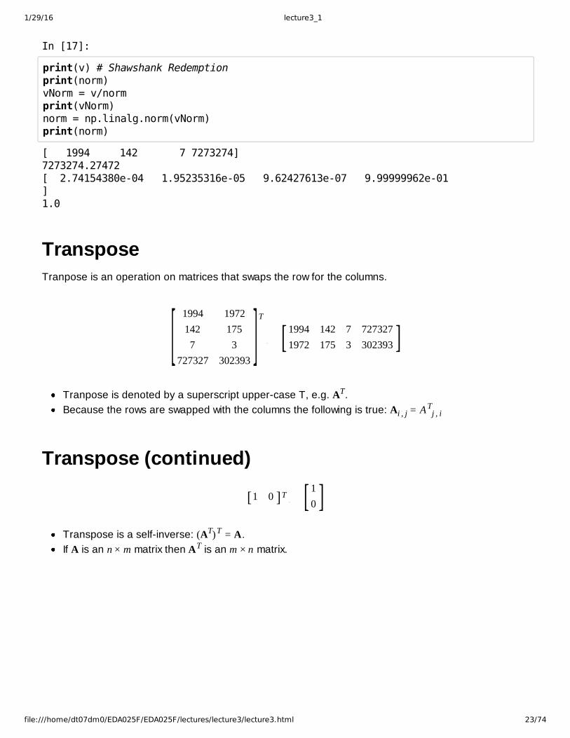
TransposeTranpose is an operation on matrices that swaps the row for the columns.

1994 1972142 1757 3

727327 302393

T

ã1994 142 7 7273271972 175 3 302393

Tranpose is denoted by a superscript uppercase T, e.g. AT.Because the rows are swapped with the columns the following is true: Ai , j = A

Tj , i

Transpose (continued)

1 0 Tã10

Transpose is a selfinverse: (AT)T = A.If A is an n × m matrix then AT is an m × n matrix.

[ ] [ ]

[ ] [ ]

1/29/16 lecture3_1


Transpose example

1994 1972142 1757 3

727327 302393

T

ã1994 142 7 7273271972 175 3 302393

To transpose a matrix you can use either np.matrix.transpose() or .T on the matrix object:

In [18]:

A = np.matrix([[1994,1972],[142,175],[7,3],[727327,302393]])At = A.T #Identical to np.matrix.transpose(A)print(A)print(At)

[[ 1994 1972] [ 142 175] [ 7 3] [727327 302393]][[ 1994 142 7 727327] [ 1972 175 3 302393]]

Scalar productGives an idea of the similarity of the vectors.Is also known as dot product or inner product.The scalar product is symbolized by the operator Î , e.g. v Î u.Only defined on vectors, of the same length.The result is a scalar.The operations are done elementwise, e.g. v Î u = k then ∑ v i × u i = k

[ ] [ ]

1/29/16 lecture3_1


Example scalar product

19721753

302393

Î

2001830559

= 1972 × 2001 + 175 × 83 + 3 × 0 + 302393 × 559 = 172998184

You can use either:np.dot() ornp.array.dot()The order of the arrays does not matter: np.dot(x, y), np.dot(y, x), x.dot(y), or y.dot(x).

In [19]:

u = np.array([1994,142,7,727327]) # Shawshank redemptionv = np.array([1972,175,3,302393]) # The Godfatherw = np.array([2001,83,0,559]) # ABC Africaprint(u.dot(v))print(v.dot(w))

219942550550172998184

Scalar product (continued)A geometric interpretation of dot product is the product between:

the length of the vectors (norm) andthe cosine of the angle between the vectors (θ).

v Î u = M v M M u M cosθ

Cosine similarityCosine similarity is defined as the cosine between the angle of the vectors (θ).Useful as a similarity measure, e.g. in natural language processing to decide closeness of twosentences.

cosine_similarity(u, v) = cosθ

[ ] [ ]

1/29/16 lecture3_1


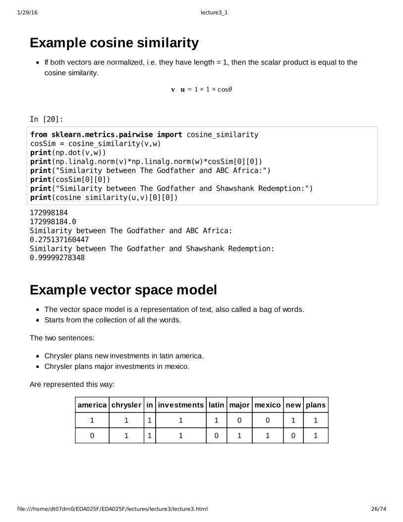
Example cosine similarityIf both vectors are normalized, i.e. they have length = 1, then the scalar product is equal to thecosine similarity.

v Î u = 1 × 1 × cosθ

In [20]:

from sklearn.metrics.pairwise import cosine_similaritycosSim = cosine_similarity(v,w)print(np.dot(v,w))print(np.linalg.norm(v)*np.linalg.norm(w)*cosSim[0][0])print("Similarity between The Godfather and ABC Africa:")print(cosSim[0][0])print("Similarity between The Godfather and Shawshank Redemption:")print(cosine_similarity(u,v)[0][0])

172998184172998184.0Similarity between The Godfather and ABC Africa:0.275137160447Similarity between The Godfather and Shawshank Redemption:0.99999278348

Example vector space modelThe vector space model is a representation of text, also called a bag of words.Starts from the collection of all the words.

The two sentences:

Chrysler plans new investments in latin america.Chrysler plans major investments in mexico.

Are represented this way:

america chrysler in investments latin major mexico new plans

1 1 1 1 1 0 0 1 1

0 1 1 1 0 1 1 0 1

1/29/16 lecture3_1


Example vector space model (continued)Using the vector space model and cosine similarity we can compute the closeness of two sentences:

In [21]:

from sklearn.feature_extraction.text import TfidfVectorizer

tfIdf = TfidfVectorizer(use_idf=False, norm=None).fit_transform( ["chrysler plans new investments in latin america", "chrysler plans major investments in mexico",])print(tfIdf.A) print(cosine_similarity(tfIdf[0],tfIdf[1])[0][0])

[[ 1. 1. 1. 1. 1. 0. 0. 1. 1.] [ 0. 1. 1. 1. 0. 1. 1. 0. 1.]]0.617213399848

Scalar matrix multiplication

2 ×1 64 8

11 ×

235

A scalar is a real number.The operation is done elementwise, e.g. k × A = C then k × a i , j = kci , j.

[ ]

[ ]

1/29/16 lecture3_1



2 ×1 64 8 =

2 × 1 2 × 62 × 4 2 × 8

11 ×

235

=

11 × 211 × 311 × 5



2 ×1 64 8 =

2 × 1 2 × 62 × 4 2 × 8 =

2 128 16

11 ×

235

=

11 × 211 × 311 × 5

=

223355


Scalar matrix multiplication example

2 ×1 64 8 11 ×

235

[ ] [ ]

[ ] [ ]

[ ] [ ] [ ]

[ ] [ ] [ ]

[ ] [ ]

1/29/16 lecture3_1


In [22]:

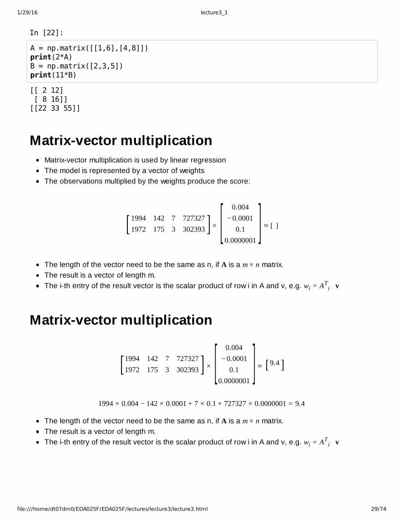
A = np.matrix([[1,6],[4,8]]) print(2*A)B = np.matrix([2,3,5]) print(11*B)

[[ 2 12] [ 8 16]][[22 33 55]]

Matrixvector multiplicationMatrixvector multiplication is used by linear regressionThe model is represented by a vector of weightsThe observations multiplied by the weights produce the score:

1994 142 7 7273271972 175 3 302393 ×

0.004−0.0001

0.10.0000001

≈ [ ]

The length of the vector need to be the same as n, if A is a m × n matrix.The result is a vector of length m.The ith entry of the result vector is the scalar product of row i in A and v, e.g. wi = A

Ti Î v

Matrixvector multiplication

1994 142 7 7273271972 175 3 302393 ×

0.004−0.00010.1

0.0000001

≈ 9.4

1994 × 0.004 − 142 × 0.0001 + 7 × 0.1 + 727327 × 0.0000001 = 9.4


Ti Î v

[ ] [ ]

[ ] [ ] [ ]

1/29/16 lecture3_1


Matrixvector multiplication

1994 142 7 7273271972 175 3 302393 ×

0.004−0.0001

0.10.0000001

≈9.48.2

1972 × 0.004 − 175 × 0.0001 + 3 × 0.1 + 302393 × 0.0000001 = 8.2


Ti Î v

Matrixvector multiplication example

1994 142 7 7273271972 175 3 302393 ×

0.004−0.0001

0.10.0000001

≈9.48.2

Instead of elementwise multiplication, as is the case for ndarray, the operator *, using the matrix class,does matrix multiplication.

In [23]:

A = np.array([[1994,142,7,7273274], [ 1972,175,3,302393 ]])v = np.matrix('0.004;-0.0001;0.1;0.0000001')print(A*v)

[[ 9.3891274] [ 8.2007393]]

Matrixmatrix multiplicationA × B = CThe ci , j entry is the dot product of the ith row in A and the jth column in BMatrixmatrix multiplication is only defined on matrices A and B, where the number of columnsin A equals the number of rows in B.If A is m × n and B is n × p then C is m × p

[ ] [ ] [ ]

[ ] [ ] [ ]

1/29/16 lecture3_1


Matrixmatrix multiplication (continued)An example of matrixmatrix multiplication:

1994 142 7 7273271972 175 3 302393 ×

0.004 1−0.0001 20.1 3

0.0000001 4

≈9.48.2


1994 142 7 7273271972 175 3 302393 ×

0.004 1−0.0001 20.1 3

0.0000001 4

≈9.48.2

1994 × 1 − 142 × 2 + 7 × 3 + 727327 × 4 = 9.4


1994 142 7 7273271972 175 3 302393 ×

0.004 1−0.0001 20.1 3

0.0000001 4

≈9.4 290953958.2 1211903

1972 × 1 − 175 × 2 + 3 × 3 + 302393 × 4 = 8.2

[ ] [ ] [ ]

[ ] [ ] [ ]

[ ] [ ] [ ]

1/29/16 lecture3_1


In [24]:

A = np.matrix([[1994,142,7,7273274], [ 1972,175,3,302393 ]])B = np.matrix('0.004,1;-0.0001,2;0.1,3;0.0000001,4')print(A*B)

[[ 9.38912740e+00 2.90953950e+07] [ 8.20073930e+00 1.21190300e+06]]

Computational complexity of matrixmultiplication

Using the definition of matrix multiplication gives an naive algorithm that takes time on theorder of n3 to multiply two n × n matrices, O(n3 ).Fastest practical algorithm is the Strassen algorithm, which only uses 7 multiplications formultiplying two 2 × 2 matrices, resulting in O(n log2 7) ≈ O(n2.8), not a big difference.Fastest theoretical is an optimized version of the Coppersmith–Winograd algorithm, with acomplexity of O(n2.373), but with a huge constant making it infeasible for matrices withreasonable sizes.

Identity matrix

I3 =

1 0 00 1 00 0 1

An identity matrix is square (n × n) with ones on the main diagonal and zeros elsewhere.Is usually denoted by In where n is the dimension.The identity matrix is the multiplicative identity for matrix multiplication, i.e. InA = AIn = A forany matrix A.

Identity matrix (continued)To utilize the identity matrix in NumPy, use np.identity(n):

[ ]

1/29/16 lecture3_1


In [25]:

I3 = np.identity(3)A = np.matrix([[2,3,5],[8,12,20],[12,18,30]])print(I3)print(A)

[[ 1. 0. 0.] [ 0. 1. 0.] [ 0. 0. 1.]][[ 2 3 5] [ 8 12 20] [12 18 30]]

In [26]:

print(I3*A)print(A*I3)

[[ 2. 3. 5.] [ 8. 12. 20.] [ 12. 18. 30.]][[ 2. 3. 5.] [ 8. 12. 20.] [ 12. 18. 30.]]

Inverse matrixInverse of a matrix A is denoted A−1.Inverses of matrices are only defined on square matrices and not all matrices are invertible.The inverse of matrix is the multiplicative inverse, i.e. AA−1 = A−1A = In.Inverting a matrix has the same computational complexity as matrix multiplication.

Example inverse matrixTo calculate the inverse of a matrix you can use np.linalg.inv() or .I on the matrix object:

1/29/16 lecture3_1


In [27]:

A = np.matrix([[2,3,4],[8,12,20],[12,19,30]])Ainv = np.linalg.inv(A) #Identical to A.Iprint(A)print(Ainv)

[[ 2 3 4] [ 8 12 20] [12 19 30]][[ 2.5 1.75 -1.5 ] [-0. -1.5 1. ] [-1. 0.25 -0. ]]

Should be equal to the identity matrix (within some numerical rounding error):

In [28]:

print((A*Ainv).round(13))

[[ 1. 0. 0.] [ 0. 1. 0.] [ 0. 0. 1.]]

SummaryMachine learning

SupervisedUnsupervised

Linear algebraMatrixVectorScalar productMatrix multiplication

First exerciseWill involve vector and matrix math, the NumPy Python package:

#### 1. Math checkup Where you will do some of the math by hand.

#### 2. NumPy and Spark linear algebra You will do some exercise using the NumPy package.

1/29/16 lecture3_1


Extra slides

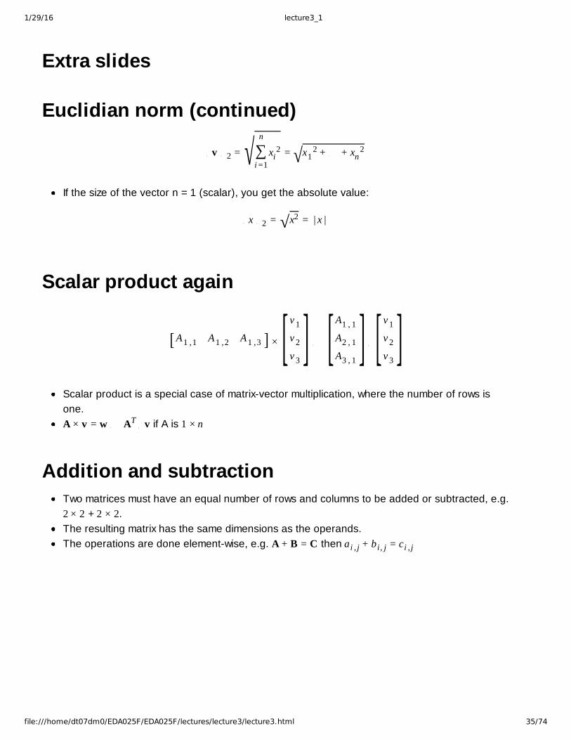
Euclidian norm (continued)

Mv M2 =n

∑i=1

xi2 = x1

2 + ø + xn2

If the size of the vector n = 1 (scalar), you get the absolute value:

Mx M2 = √x2 = | x |

Scalar product again

A1 ,1 A1 ,2 A1 ,3 ×

v 1v 2v 3

ã

A1 , 1A2 , 1A3 , 1

Î

v 1v 2v 3

Scalar product is a special case of matrixvector multiplication, where the number of rows isone.A × v = w ã AT Î v if A is 1 × n

Addition and subtractionTwo matrices must have an equal number of rows and columns to be added or subtracted, e.g.2 × 2 + 2 × 2.The resulting matrix has the same dimensions as the operands.The operations are done elementwise, e.g. A + B = C then a i , j + b i , j = ci , j

√ √

[ ] [ ] [ ] [ ]

1/29/16 lecture3_1


Addition and subtraction (continued)Example of addition:

2 53 7 +

1 64 8

Example of subtraction:

57 −

14


2 53 7 +

1 64 8 =

2 + 1 5 + 63 + 4 7 + 8


57 −

14 =

5 − 17 − 4


2 53 7 +

1 64 8 =

2 + 1 5 + 63 + 4 7 + 8 =

3 117 15


57 −

14 =

5 − 17 − 4 =

43

[ ] [ ]

[ ] [ ]

[ ] [ ] [ ]

[ ] [ ] [ ]

[ ] [ ] [ ] [ ]

[ ] [ ] [ ] [ ]

1/29/16 lecture3_1


In [29]:

A = np.matrix([[2,5],[3,7]])B = np.matrix([[1,6],[4,8]])print(A+B) C = np.array([5,7])D = np.array([1,4])print(C-D)

[[ 3 11] [ 7 15]][4 3]

Matrixmatrix multiplication (continued)Some properties of matrix multiplication:

Is an associative operation, rearranging the parentheses in such an expression will not changeits value, e.g. A(BC) = (AB)CIs not a commutative operation, the order of the operands matter, e.g. generally AB ≠ BAThe transpose of AB is the tranpose of B multiplied by the transpose of A, e.g. ABT = BTAT

Outer productThe operation is symbolized by à , e.g. v à w = AIs defined on two vectors and the result is a matrix.Is a special case of matrix multiplication: và w = vwT = A, i.e. a i , j = v iwj

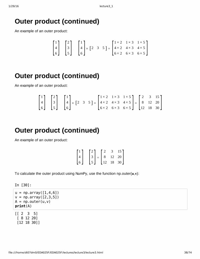
Outer product (continued)An example of an outer product:

146à

235ã

146

× 2 3 5[ ] [ ] [ ] [ ]

1/29/16 lecture3_1



146à

235ã

146

× 2 3 5 =

1 × 2 1 × 3 1 × 54 × 2 4 × 3 4 × 56 × 2 6 × 3 6 × 5


146à

235ã

146

× 2 3 5 =

1 × 2 1 × 3 1 × 54 × 2 4 × 3 4 × 56 × 2 6 × 3 6 × 5

=

2 3 158 12 2012 18 30


146à

235

=

2 3 158 12 2012 18 30

To calculate the outer product using NumPy, use the function np.outer(u,v):

In [30]:

u = np.array([1,4,6])v = np.array([2,3,5])A = np.outer(u,v)print(A)

[[ 2 3 5] [ 8 12 20] [12 18 30]]

[ ] [ ] [ ] [ ] [ ]

[ ] [ ] [ ] [ ] [ ] [ ]

[ ] [ ] [ ]

1/29/16 lecture3_1


Supervised learning and regression

Today's scheduleOverview of machinelearning and linear algebra.Exercise in linear algebra.Regression and ML pipeline. <Exercise in linear regression.Classification and logistic regression.Exercise in logistic regression.

Regression

RegressionTo learn a model that predicts a continuous label, i.e. a numeric value, from observations (features).

Examples of values that can be predicted:

Age of a person from his/her shoe size, length,etc.Price of a car from manufacturer, country ofpurchase, etc.IMDb score of a movie from year, director, etc.

1/29/16 lecture3_1


Linear regressionEach observation is represented by a label y and a feature vector x:

y 0 R xT = x1 x2 x3 … xi

We assume that there exists a linear mapping between the features and the label:

y ≈ y = w0 + w1x1 + w2x2 + w3x3 +… + wixi

Linear regression (continued)If we extend the feature vector with a constant x0 = 1, we get the following:

xT = 1 x1 x2 x3 … xi

And let the weights be the vector w:

wT = w0 w1 w2 w3 … wi

And then we can write the linear mapping as the following scalar product:

y ≈ y =n

∑i=1

wixi = w Î x

Linear regression (continued)The model (w) enables us to predict the IMDb score from the observations (x):

1 1994 142 7 7273271 1972 175 3 302393 ×

00.004

−0.00010.1

0.0000001

≈9.48.2

[ ]

[ ]

[ ]

[ ] [ ] [ ]

1/29/16 lecture3_1


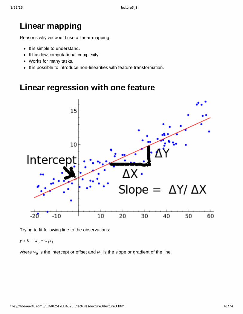
Linear mappingReasons why we would use a linear mapping:

It is simple to understand.It has low computational complexity.Works for many tasks.It is possible to introduce nonlinearities with feature transformation.

Linear regression with one feature

Trying to fit following line to the observations:

y ≈ y = w0 + w1x1

where w0 is the intercept or offset and w1 is the slope or gradient of the line.

1/29/16 lecture3_1


Representing an observation: regressionMLlib's represents a data point with the class LabeledPoint(label, features), which consists of thefollowing:

A label, represented by a real value.A list of features.

In [15]:

LabeledPoint(9.3, [1994,142,7,727327]) #Shawshank Redemption

Out[15]:

LabeledPoint(9.3, [1994.0,142.0,7.0,727327.0])

Representing an observation (continued)The feature vector can be inputed in one of the following formats:

A list.NumPy array.SparseVector, if we have many zeros.DenseVector, a NumPy compatible MLib representation.

Sparse representationEncodes only the nonzero elements.Efficient storage if it has got many zeros.Consists of:

the lengthindices of nonzero elementsthe values

In [23]:

vecA = [ 0, 2, 1, 0, 1, 3, 0, 2, 0, 0]vecB = [ 0, 0, 0, 1, 1, 2, 1, 2, 0, 0]

vecASparse = (10,[1,2,4,5,7],[2.0,1.0,1.0,3.0,2.0])vecBSparse = (10,[3,4,5,6,7],[1.0,1.0,2.0,1.0,2.0])

1/29/16 lecture3_1


Representing an observation: classificationIn the case of a classification, the label is a class:

0 (negative) and 1 (positive) for binary.0,1,2,... for multiclass.

In [16]:

LabeledPoint(1, [36961, 2503]) #Salammbô first chapter French

Out[16]:

LabeledPoint(1.0, [36961.0,2503.0])

Example of LabeledPointIn [17]:

from pyspark.mllib.regression import LabeledPointimport numpy as np#Create a 10000x4 matrix with random numbers randomMatrix = np.random.rand(10000, 4) print(randomMatrix[0])printobs = sc.parallelize(randomMatrix)#Take first number as label, rest as feature vectorobs = obs.map(lambda x: LabeledPoint(x[0], x[1:])) print(obs.take(1)[0].label, obs.take(1)[0].features)

[ 0.5735422 0.90549853 0.10395045 0.5981861 ]

(0.5735421994807254, DenseVector([0.9055, 0.104, 0.5982]))

Evaluating regressionWe can measure the closeness between the labels (yi) and the predictions (yi) with the followingperformance measures:

Mean absolute error (MAE):

1n

n

∑i=1

| yi − yi |

1/29/16 lecture3_1


Evaluating regression (continued)Mean squared error (MSE):

1n

n

∑i=1

(yi − yi)2

Has nice mathematical properties, as we soon will see.

Evaluating regression (continued)Root mean squared error (RMSE):

1n

n

∑i=1

(yi − yi)2,

which has the same unit as the quantity being estimated, e.g. IMDb score instead of IMDb score2. It isusually slightly higher than MAE.

Evaluating using MLlibIn MLlib you can use the RegressionMetrics class to calculate the previously mentionedperformance measures. It takes a RDD of (prediction, label) pairs as an argument.

The following variables are than available from the class:

meanAbsoluteErrormeanSquaredErrorrootMeanSquaredError

An example will follow after we introduce LinearRegressionWithSGD.

√

1/29/16 lecture3_1


Linear least squaresLet us first define some mathematical objects:

n is the number of observations.d is the number of features.X 0 Rn× d Matrix containing the observations.y 0 Rn The labels.w 0 Rd The weights of the model.y = Xw 0 Rn The predictions.

Linear least squares (continued)We want to learn a model w, that tries to minimize the MSE:

minw

1n

n

∑i=1

(yi − yi)2 = min

w

1n

n

∑i=1

(yi − wxi)2 ã min

wM y − XwM22

It has the following closed form solution, if the inverse exist:

w = (XTX) −1XTy

Ridge regressionWe want the model to generalize well, i.e. predict unseen data correctly.

Least squares tries to minimize the error on the training data and it could overfit.

A simpler model may be less prone to overfitting.A model with smaller weights is simpler.

1/29/16 lecture3_1


Ridge regression (continued)We can introduce a term representing the model complexity, represented by the square of the normof the weights:

minwM y − Xw M22 + λ M wM

22

Where λ is a tunable parameter, to trade off model complexity with training error.

It has the following closed form solution, if the inverse exists:

w = (XTX + λId)−1XTy

Optimizing linear regressionWe saw a closed form solution that minimizes My − XwM22

If the number of features is large, this solution is unusable.We need to iteratively solve the problem.

Gradient descent is an iterative way to optimize the function.

Least squares with gradient descentThe iterative solution is given by this update formula:

wi+1 = wi − αi

n

∑i= j

(wix j − yj)x j

It has the parameter α (step size), which decides how big the jump for each iteration is.

(see "Extra slides: gradient descent" for more information)

Choosing the α (step size)If you choose an alpha (step size) that is:

Smaller than needed, you will converge slowly.Larger than needed, it is possible to overshoot the target and even diverge.

1/29/16 lecture3_1


Choosing the α (continued)It is possible to change the α during the descent, so that it will decrease with the number ofiterations.

This will make the jumps smaller the closer you come to the solution.

αi =αn√i

In the equation:

α is a constant.n is the number of observations.i is the number of iterations.

Linear regression with stochastic gradient descent(SGD)

The MLib implementation of stochastic gradient descent uses a simple (distributed) samplingof the data examples.Calculating the true gradient, would require access to the full data set, instead we use afraction of the data.For each iteration, a computation of the sum of the partial results is performed.

Linear regression with Stochastic Gradient Descent(continued)The advantages of SGD are:

Efficiency.Can handle large amount of features and observations.

The disadvantages are:

Requires several hyperparameters, e.g. step size or regularization.Sensitive to feature scaling.

1/29/16 lecture3_1


SGD with MLlibThe class that trains linear regression with stochastic gradient descent is calledLinearRegressionWithSGD.

The class has the method train(), which returns a LinearRegressionModel, the method has thefollowing arguments:

data – The training data, an RDD of LabeledPoint.Optional:

iterations – The number of iterations.step – The step parameter used in SGD.miniBatchFraction – Fraction of data to be used for each iteration.initialWeights – The initial weights.

SGD with MLlib (continued)Optional arguments continued:

regParam – The regularizer parameter.regType – The type of regularizer used for training our model.

“l1” for using L1 regularization (lasso).“l2” for using L2 regularization (ridge).None for no regularization.

intercept – Boolean parameter, to use an intercept.validateData – Boolean parameter, to validate data.

SGD exampleIn the following example I will do the following:

Reuse the observations that was created in a previous example.It contains 10000 observations with a label and 3 features.The numbers are all uniformly distributed between 0 and 1.

Split the data set into a 75% training set and 25% validation set.

1/29/16 lecture3_1


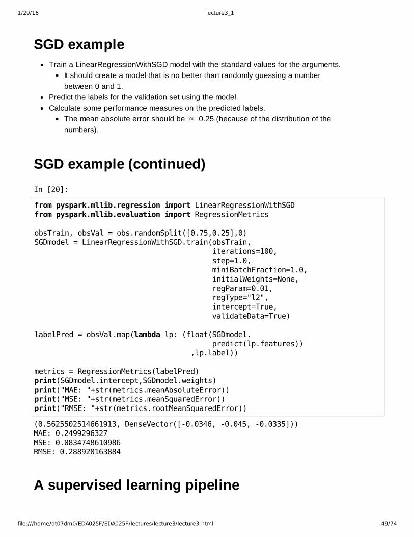
SGD exampleTrain a LinearRegressionWithSGD model with the standard values for the arguments.

It should create a model that is no better than randomly guessing a numberbetween 0 and 1.

Predict the labels for the validation set using the model.Calculate some performance measures on the predicted labels.

The mean absolute error should be ≈ 0.25 (because of the distribution of thenumbers).

SGD example (continued)In [20]:

from pyspark.mllib.regression import LinearRegressionWithSGDfrom pyspark.mllib.evaluation import RegressionMetrics

obsTrain, obsVal = obs.randomSplit([0.75,0.25],0)SGDmodel = LinearRegressionWithSGD.train(obsTrain, iterations=100, step=1.0, miniBatchFraction=1.0, initialWeights=None, regParam=0.01, regType="l2", intercept=True, validateData=True)

labelPred = obsVal.map(lambda lp: (float(SGDmodel. predict(lp.features)) ,lp.label))

metrics = RegressionMetrics(labelPred) print(SGDmodel.intercept,SGDmodel.weights)print("MAE: "+str(metrics.meanAbsoluteError))print("MSE: "+str(metrics.meanSquaredError))print("RMSE: "+str(metrics.rootMeanSquaredError))

(0.5625502514661913, DenseVector([-0.0346, -0.045, -0.0335]))MAE: 0.2499296327MSE: 0.0834748610986RMSE: 0.288920163884

A supervised learning pipeline

1/29/16 lecture3_1


Supervised learning pipelineStarts out as raw data.

Raw dataYou need to collect the data somehow, e.g:

Record which ads an user clicks on.Crawl the IMDb website.Get patient data from a registry.

Real world data tends to be "dirty".

Supervised learning pipeline (continued)Starts out as raw data.Preprocessing data.

Preprocessing dataA tip is to do an ocular inspection (on samples) of the data set before starting thepreprocessing procedure.You often see if something obivious stands out on the data, e.g. if a variable is coded wrongor if a feature has many missing values.

Then you may want to do any of the following steps:

Formatting the data.Removing corrupt data.Handle missing values:

Remove observations with missing data.Impute the missing value.

Converting the data, e.g. Yes > 1, No > 0.Sampling the data.

1/29/16 lecture3_1


Supervised learning pipeline (continued)Starts out as raw data.Preprocessing data.Feature extraction.

Extracting featuresCreating the possible features (feature engineering) that are going to be used to train themodel.This can be done as a part of the preprocessing step or on the fly by the program.

Some ways of creating the features:

Using the data as it is.Changing the unit of the data, e.g. creatinine from mg/dl to μmol/l.Using onehot encoding to represent categorical data.Using bagofwords to represent text.

Extracting features (continued)Creating categorical data from real valued, e.g angle ( @ ) to direction (N,S,W,E).Using mathematical functions, e.g. √x or sin(x).Combining features:

Creating polynomial features, e.g. x 2 or xy.Using binary operators, e.g. AND or XOR.Using any combination of mathematical functions.

Supervised learning pipeline (continued)Starts out as raw data.Preprocessing data.Feature extraction.Transformation of features.

1/29/16 lecture3_1


Scaling and normalizingThe idea is to scale/standardize/normalize the features so they become more homogeneous.This may:

Improve the prediction result.Speed up the training of the model.

In the IMDB data set, the box office feature outweights the number of Oscars for example.

A =1994 142 7 7273271972 175 3 302393

This means that the norm of an observation will likely to be equal to this feature.The idea is to normalize the features so they become more homogeneous.

Scaling and normalizing (continued)Rescaling a feature, i.e. scaling the feature to the interval [0,1]:

x ′ =x − min (x)max x − min x

Standardizing a feature, i.e. that the feature has zeromean and unitvariance:

x ′ =x − xσ

Scaling and normalizing (continued)Normalizing a feature vector, i.e. making the feature vector have unit length in the norm(usually the euclidan norm, i.e p = 2):

Mv Mp = (n

∑i=1

| xi |p)1 /p v ′ =

vMvMp

M v ′ M = 1

[ ]

1/29/16 lecture3_1


Scaling and normalizing with MLlibMLlib has two classes representing feature standardization and normalizing: StandardScaler andNormalizer.

The StandardScaler takes an RDD[Vector] as input, using the fit() and the transform()methods, learns the summary statistics, and then returns a standardized data set.

x ′ =x − xσ

The Normalizer takes a float p and then transforms individual feature vectors to have unit pnorm.

Mv Mp = (n

∑i=1

| xi |p)1 /p v ′ =

vMvMp

M v ′ M = 1

Scaling and normalizing exampleIn [19]:

from pyspark.mllib.feature import StandardScalerfrom pyspark.mllib.feature import Normalizer

features = sc.parallelize([[666,1337,1789],[1066,21,1],[1,3,5]])

scaler = StandardScaler().fit(features)scaledFeatures = scaler.transform(features)print(scaledFeatures.collect())printnorm = Normalizer(float('inf'))normScaledFeatures = norm.transform(scaledFeatures)print(normScaledFeatures.collect())

[DenseVector([1.238, 1.7476, 1.735]), DenseVector([1.9815, 0.0274, 0.001]), DenseVector([0.0019, 0.0039, 0.0048])]

[DenseVector([0.7084, 1.0, 0.9928]), DenseVector([1.0, 0.0139, 0.0005]), DenseVector([0.3834, 0.8087, 1.0])]

1/29/16 lecture3_1


Supervised learning pipeline (continued)Starts out as raw data.Preprocessing data.Feature extraction.Transformation of features.Supervised learning.

Learning a modelTrain a model on your training set, e.g. using any of these algorithms:

Regression.Linear (lasso/ridge).Nonlinear.Regression trees.

Classification (will go through in next lecture).

Learning a model (continued)Both.

Random forest.Artificial neural network (ANN).Support vector machine (SVM).

Supervised learning pipeline (continued)Starts out as raw data.Preprocessing data.Feature extraction.Transformation of features.Supervised learning.Evaluation.

1/29/16 lecture3_1


EvaluationEvaluate on your validation set, and then test set, if you created one.Possibly use cross validation, instead of a validation set.Either way you need a performance meassure/metric, e.g. using any of these:

Mean absolute error (MAE).Mean squared error (MSE).Root mean squared error (RMSE).


Feature extraction.Transformation of features.Supervised learning.Evaluation.

Possible reiteration (of the above steps).

Reiteration/optimizationYou usually want to reiterate through some of the previously mentioned steps, to be able to improvethe prediction of unseen examples, which we estimate by predicting the validation set and thenapplying an appropriate evaluation metric.

Changes that may improve the result includes:

The features being used (the feature set).The scaling and normalization of features.The algorithm to create the model.Hyperparameters of the model.

1/29/16 lecture3_1


Tuning of the hyperparametersFor example:

LinearRegressionWithSGD has a number of hyperparameters, e.g. the number of iterationsand the step size.These parameters can sometimes greatly influence the quality of the model.You want to optimize the model with the best choice of these arguments.Crossvalidation is often used to estimate this performance.

Tuning of the hyperparameters (continued)Grid search is an exhaustive search, which may be computationally infeasible, if the parameters aresomewhat independent of each other, it is possible to tune on at a time:

Optimizing one parameter at a time.Choose reasonable starting values for the parameters.Tune one parameter.Evaluate on validation data.Fix the best parameter value.May need to reiterate for some parameters.


Feature extraction.Transformation of features.Supervised learning.Evaluation.

Possible reiteration (of the above steps).Prediction.

1/29/16 lecture3_1


PredictionOnce the model is ready you can predict:

I.e. apply the model to an unseen observation.E.g. predicting if a patient has cancer or not.You may want to reserve a test set from the original data, to be able to estimate thegeneralization of the model.

SummaryRegression

EvaluationGradient descentSGD with MLlib

Supervised learning pipelineExtract featuresScaling and normalizingLearning a modelEvaluate / reiterate

Second exerciseWill involve linear regression with stochastic gradient descent and with MLlib.

This exercise will be divided into three parts:

#### 1. Importing and preparing the data#### 2. Creating a baseline benchmark#### 3. Utilizing MLlib

1/29/16 lecture3_1


Parkinsons Telemonitoring Data SetA data set from the UCI Machine Learning Repository.Unified Parkinson’s Disease Rating Scale (UPDRS)

Measures a person's progress in the disease in a scale from 0 to 176.Has about 6000 observations and 26 features, which are numerical and taken from voicesamples.Your task is to correctly predict the UDPRSscore based on these voice measures.The performance metric is the mean absolute error (MAE).

Extra slides: gradient descent (they got missingimages)

Convex functionA convex function is Ushaped, which means that there only exist one local minimum and it is theglobal minimum.

Nonconvex functionA non convex function may have several local minima, which are not the the global minimum.

ConvextivityFortunately Least Squares, Ridge Regression and Logistic Regression are all convex minimizationproblems.

Gradient descent (continued)First pick an arbitrary starting point.Iterate:

Decide a descent direction.Pick a step size.Update.

Until stoping criterion is satisfied.

1/29/16 lecture3_1


Deciding the descent directionBecause it is a convex function, the direction of descent is the negtive slope.

This gives the following update rule:

wi+1 = wi − αidfdw

(wi)

Least squares with gradient descentUsing least squares as the function gives the following update rule:

wi+1 = wi − αidfdw

(wi) = wi − αidfdw

(n

∑j=1

(wix j − yj)2) ã

Using the chain rule gives the following formula:

wi+1 = wi − αi

n

∑i= j

(wix j − yj)x j

Evaluation (continued)Classification.

Confusion matrix.Accuracy.Precision, recall, and F1.

Receiver operator characteristic (ROC).Area under ROC (AUROC).

Tuning of the hyperparameters (continued)Grid search

Define and discretize the search space (linear or log scale), e.g:iter 0 10, 50, 100, 500, 1000α 0 1, 2, 3, 4, 5

Test all ntuples in the cartesian set of the parameters, e.g:para 0 iter × α = (1, 10), (1, 50), …|para| = 25

1/29/16 lecture3_1


Grows quickly with the number of parameters.Evaluate on the validation data.

Classification and logistic regression

Today's scheduleOverview of machinelearning and linear algebra.Exercise in linear algebra.Regression and ML pipeline.Exercise in linear regression.Classification and logistic regression. <Exercise in logistic regression.

ClassificationTo learn a model that predicts a categorical label, i.e. a discrete value, which may be binary (1 or0), or multiclass (1,2,3,...) from observations (features).

Examples of values that can be predicted:

An email as either spam or not spam, fromthe subject, body of the mail, etc.A patient as having cancer or not cancer,from the age, blood values, etc.A customer as having low, medium, or highinterest, from click patterns, buying patterns,etc.

Features

1/29/16 lecture3_1


Types of dataThe raw data may contain several types of information, for example:

Numeric, e.g. age or blood creatinine value.Binary, e.g. gender or apple/pc user.Categorical, e.g. country or car brand.

Ordinal, e.g. customer interest (low, medium, high)Text, e.g. body of an email or wikipedia article.

Ordinal variablesFor ordinal variables, there exists an ordering of the categories, e.g. high > low, but usually nomeasure of closeness.

We can represent the variable as a single numerical feature, e.g. low = 1, medium = 2, and high =3

Then we introduce a degree of closeness, which may or may not be desirable.Or we can use onehot encoding (a way to represent nominal/categorical data).

Categorical variablesFor categorical variables, there is no intrinsic ordering or measure of closeness, you can not saythat Germany > France.

We could represent the variable as a single numerical feature, e.g. Germany = 0, France = 1,Belgium = 2

Then we introduce both an ordering and a degree of closeness, which usually is notdesirable.Better to use onehot encoding!

1/29/16 lecture3_1


Onehot encoding (OHE)Also called dummy encoding.Create a vector of binary features, where one of them is equal to 1 and rest is 0

Where the index in the vector represents the category value.Like in C bit field encoding.This does not introduce spurious relationships between the categories.Exist in MLib from version 1.4 as OneHotEncoder.

For example:Germany = 0, France = 1, Belgium = 2 → Germany = [1,0,0] France = [0,1,0] Belgium = [0,0,1]

Example of OHEIn [1]:

'Belgium': 2, 'Sweden': 3, 'Germany': 0, 'Russia': 4, 'France': 1Sweden = [ 0. 0. 0. 1. 0.]France = [ 0. 1. 0. 0. 0.]

Text dataA way to represent text data is to use the bagofwords representation:

First create a dictionary of the words similar to OHE encoding.Instead of binary values for the indices, we store a number corresponding to thefrequency of the word in that observation.

This usually results in quite sparse feature vectorThe number of unique words in the English language is over 1 million, althoughall words are not used in any corpus.

1/29/16 lecture3_1


Example of bag of wordsText 1: John likes to watch movies. Mary likes movies too.Text 2: John also likes to watch football games

John = 0, likes = 1, to = 2, watch = 3, movies = 4, also = 5, football = 6, games = 7, Mary = 8, too= 9 →

Encoding of text 1: [1, 2, 1, 1, 2, 0, 0, 0, 1, 1]Encoding of text 2: [1, 1, 1, 1, 0, 1, 1, 1, 0, 0]

The element values are called the term frequency (TF).

Feature hashingUse a hash function to calculate the index of the token, modulus the length of thedesired vector.

This is less memory and computationally expensive then creating a dictionary.

If the hash function is a reasonable one, the distribution of tokens should be somewhatuniform.

This can reduce the dimension of the feature vector considerably.Which possibly could create collisions, which may lower the quality of the model.

HashingTFIn Mllib there exist a class, called HashingTF

It represents feature hashing and the counting of the frequencies of thehashes.The class takes as argument the number of features.It has got the method transform(), that takes the input dataset and return anRDD of SparseVector:s.

Example of feature hashing using TF

1/29/16 lecture3_1


In [2]:

(10,[1,2,4,5,7],[2.0,1.0,1.0,3.0,2.0])(10,[3,4,5,6,7],[1.0,1.0,2.0,1.0,2.0])[ 0. 2. 1. 0. 1. 3. 0. 2. 0. 0.][ 0. 0. 0. 1. 1. 2. 1. 2. 0. 0.]

Inverse document frequency (IDF)Term frequency (TF) is used to measure the importance.It is easy to overemphasize terms that appear very often, e.g. “a”, “the”, and “of”.If a term appears very often across the corpus, it means it does not carry specialinformation.Inverse document frequency (IDF) is a numerical measure of how much information aterm provides.IDF is defined as the inverse of the number of documents that contain the term.The TF multiplied by the IDF is often called TFIDF.

TFIDFIn Mllib there exist a class, called IDF, that represents the TDIDF model.

It needs to do a pass through the data first to calculate the IDF.Then you can use the method transform(HashingTF), that multiplies the TFwith the IDF.

Example of IDFIn [4]:

(10,[1,2,4,5,7],[2.0,1.0,1.0,3.0,2.0])(10,[3,4,5,6,7],[1.0,1.0,2.0,1.0,2.0])(10,[1,2,4,5,7],[0.810930216216,0.405465108108,0.0,0.0,0.0])(10,[3,4,5,6,7],[0.405465108108,0.0,0.0,0.405465108108,0.0])

1/29/16 lecture3_1


0

0.5

1

−6 −4 −2 0 2 4 6

Logistic regressionThe following equation is the logistic function:

σ(t) =1

1 + e− t

Logistic regression (continued)If t is a linear combination of weights, i.e. t = w Î x we get the following equation:

σ(t) =1

1 + ew0+w1x1 + … +wixi

σ(t) is between 0 and 1 for every t, for positive infinity it is equal to 1 and for negative it is 0. It istherefore interpretable as a probability.

1/29/16 lecture3_1


Logistic regression (continued)To go from a probability to a binary classification we use a threshold, often 0.5.

If it is over the treshold we classify it as positive.

σ(t) ≥ 0.5 ã 1

If it is under we classify it as negative.

σ(t) < 0.5 ã 0

Logistic regression with limitedmemory BFGS(LBFGS)There exists a SGD variant of logistic regression in MLlib also, but the LBFGS tends to be bothfaster and use less memory.

It is an optimization algorithm in the family of quasiNewton methods that approximates theBroyden–Fletcher–Goldfarb–Shanno (BFGS) algorithm using a limited amount of computermemory.

LBFGS with MLlibThe class that trains logistic regression with LBFGS is called LogisticRegressionWithLBFGS. Theclass has the method train, which returns a LogisticRegressionModel, the method has thefollowing arguments:

data – The training data, an RDD of LabeledPoint.Optional:

iterations – The maximum number of iterations.initialWeights – The initial weights.corrections – The number of corrections used in the LBFGS update.tolerance – The convergence tolerance of iterations for LBFGS

1/29/16 lecture3_1


LBFGS with MLlib (continued)Optional continued:

regParam – The regularizer parameter.regType – The type of regularizer used for training our model.

“l1” for using L1 regularization (lasso).“l2” for using L2 regularization (ridge).None for no regularization.

intercept – Boolean parameter, to use an intercept.validateData – Boolean parameter, to validate data.numClasses – The number of classes a label can take.

Example of LBFGSIn [5]:

[-0.258464021679,0.740603840877,-0.671843280475,0.805617017835,-0.469895541298,0.134604891419,-0.407452394167,-1.27835829141,0.572797907614]0.170672270554

1/29/16 lecture3_1


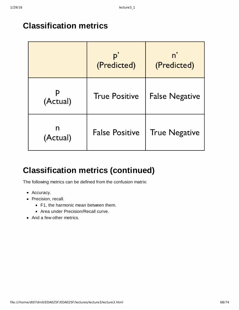
Classification metrics

Classification metrics (continued)The following metrics can be defined from the confusion matrix:

Accuracy.Precision, recall.

F1, the harmonic mean between them.Area under Precision/Recall curve.

And a few other metrics.

1/29/16 lecture3_1


Receiver operating characteristic (ROC)

1/29/16 lecture3_1


ROC (continued)The ROC is a graph over true positive rate/false positive rate (can be defined from the confusionmatrix).

The area under the ROC graph can be interpeted as the probability that as randomly chosenpositive example > negative example.

A model that assigns random labels to observations has an AUROC of 0.5.A perfect model has an AUROC of 1.0A reasonable model should therefore have an AUROC between 0.5 and 1.0

BinaryClassificationMetricsIn MLlib there exist a class called BinaryClassificationMetrics, that takes a pair RDD of predictedlabels and true labels, and then has the following methods:

areaUnderPR(): Computes the area under the precisionrecall curve.areaUnderROC(): Computes the area under the ROC curve.

Before using it you need call clearThreshold() on the model to remove the classification and getthe raw probability.

Example of AUROCIn [7]:

[(0.43377292697214964, 1.0), (0.30489754918354856, 0.0), (0.41113216061927377, 1.0), (0.4474745011380102, 0.0), (0.2708764900478493, 0.0), (0.3322889798311969, 1.0), (0.6380750346426529, 1.0)]

The AUROC of random features: 0.538194444444

The AUPR of random features: 0.608066661347

1/29/16 lecture3_1


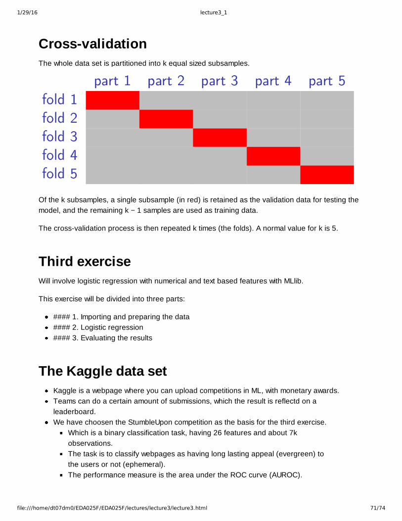
CrossvalidationThe whole data set is partitioned into k equal sized subsamples.

Of the k subsamples, a single subsample (in red) is retained as the validation data for testing themodel, and the remaining k − 1 samples are used as training data.

The crossvalidation process is then repeated k times (the folds). A normal value for k is 5.

Third exerciseWill involve logistic regression with numerical and text based features with MLlib.

This exercise will be divided into three parts:

#### 1. Importing and preparing the data#### 2. Logistic regression#### 3. Evaluating the results

The Kaggle data setKaggle is a webpage where you can upload competitions in ML, with monetary awards.Teams can do a certain amount of submissions, which the result is reflectd on aleaderboard.We have choosen the StumbleUpon competition as the basis for the third exercise.

Which is a binary classification task, having 26 features and about 7kobservations.The task is to classify webpages as having long lasting appeal (evergreen) tothe users or not (ephemeral).The performance measure is the area under the ROC curve (AUROC).

1/29/16 lecture3_1


The Kaggle data set (continued)

Imputation of variablesIf you use real world data, and in this exercise, it is likely that you will encounter missing featurevalues, often represented in the data as:

"" (the empty string)?NA

There can be missing values, because in the real world, for various reasons there is not alwayscomplete information available, e.g:

some value was not recorded at collection timeis not applicable to that data point

1/29/16 lecture3_1


Imputation of variables (continued)Ways of handling observations with missing data

Casewise deletion: delete the observations that has missing values.This effectively reduces the size of the data set.If the missing values are random, no bias is introduced in the model.However missing values rarely tend to be completely random.

Imputation of variables (continued)Mean/mode imputation: replace the missing value with the mean for real valued featuresand mode for categorical.

Has the property that the sample mean for that variable is unchanged.But this can severely distort the distribution for this variable.Distorts relationships between variables by “pulling” estimates of the correlationtoward zero.

This is the one you will use in the exercise.

Imputation of variables (continued)Hotdeck imputation: replacing the missing value from a uniform distribution of the nonmissing values.

Has the property that the the distribution for that variable is unchanged.

Using a model: replace the missing values based on a model created on the othervariables.

Works good if the variable is correlated with the other variables.

Extra slides

1/29/16 lecture3_1


Exhaustive crossvalidationLeaveoneout crossvalidation (LOCV) involves using one observation as the validation set andthe remaining observations as the training set.

This is repeated on all ways to cut the original sample on a validation set of one observation anda training set. And then calculating the mean validation metric over all partitions.

So as soon as the number of observations is quite big it becomes infeasible to calculate.

kfold crossvalidationThe original sample is randomly partitioned into k equal sized subsamples. Of the k subsamples,a single subsample is retained as the validation data for testing the model, and the remaining k −1 samples are used as training data.

The crossvalidation process is then repeated k times (the folds), with each of the k subsamplesused exactly once as the validation data.

A normal value for k is 10. When k = the number of observations, the kfold crossvalidation isexactly the leaveoneout crossvalidation.

week 3: supervised learning today's lectures - the semantica...

Documents