week 11 image compression - canerozcan.netcanerozcan.net/files/cme429_week10.pdf · image...
TRANSCRIPT
CME429 Introduction to Image Processing
Assist. Prof. Dr. Dr. Caner ÖZCAN
Week 11 Image Compression
But life is short and information endless ... Abbreviation is a necessary evil and the abbreviator's business is to make the best of a job which, although
intrinsically bad, is still better than nothing. ~Aldous Huxley

Outline
2
8. Image Compression ►Fundamentals
►Some Basic Compression Methods
►Digital Image Watermarking
Relative Data Redundancy
3
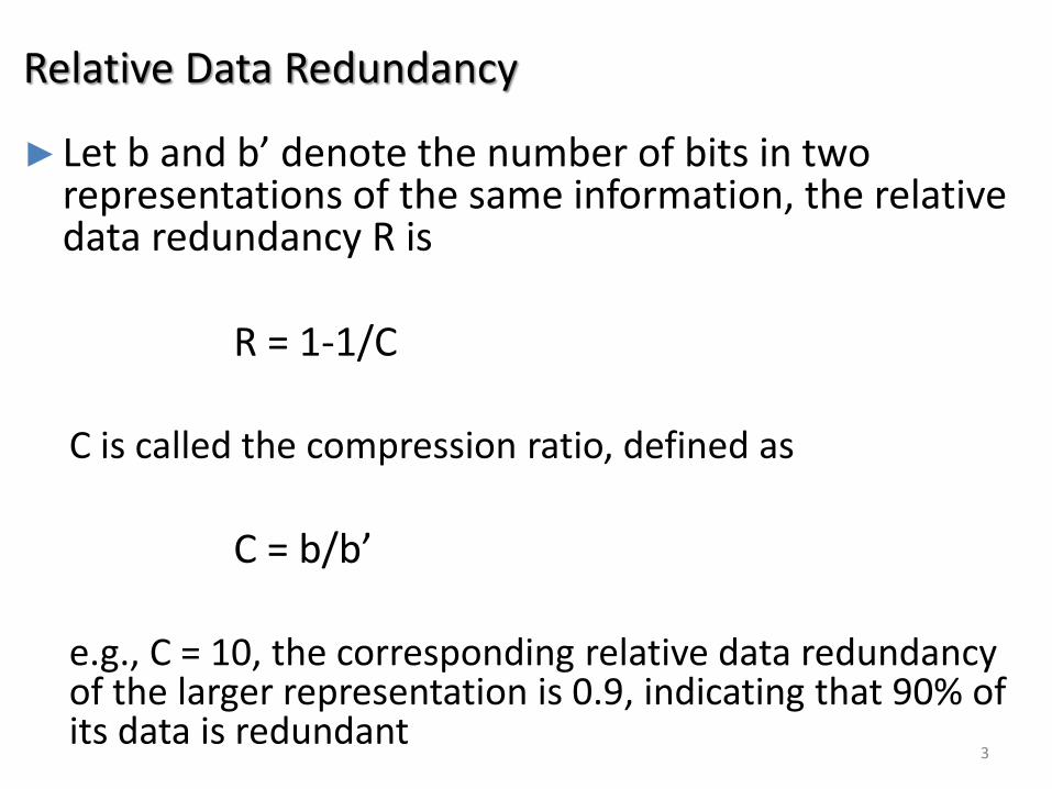
►Let b and b’ denote the number of bits in two representations of the same information, the relative data redundancy R is
R = 1-1/C C is called the compression ratio, defined as
C = b/b’
e.g., C = 10, the corresponding relative data redundancy of the larger representation is 0.9, indicating that 90% of its data is redundant

Why do we need compression?
4
►Data storage
►Data transmission
How can we implement compression?
5
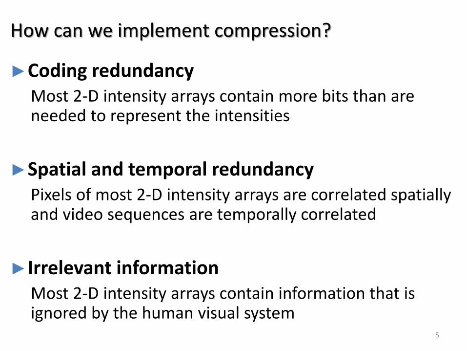
►Coding redundancy Most 2-D intensity arrays contain more bits than are needed to represent the intensities
►Spatial and temporal redundancy Pixels of most 2-D intensity arrays are correlated spatially and video sequences are temporally correlated
►Irrelevant information Most 2-D intensity arrays contain information that is ignored by the human visual system

Examples of Redundancy
6

Image Compression Standards
7

8

9
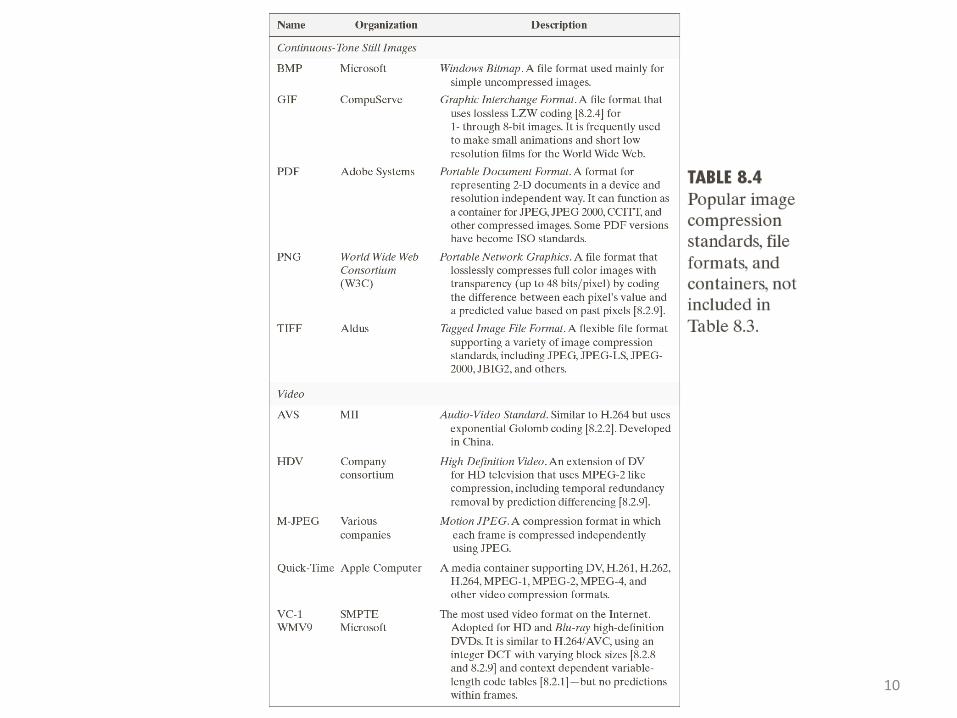
10
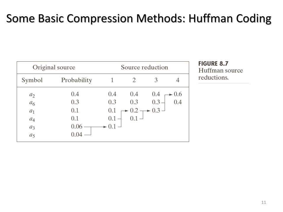
Some Basic Compression Methods: Huffman Coding
11

Some Basic Compression Methods: Huffman Coding
12
The average length of this code is
0.4*1 0.3*2 0.1*3 0.1*4 0.06*5 0.04*5
= 2.2 bits/pixel
avgL

CME429 Introduction to Image Processing
Assist. Prof. Dr. Dr. Caner ÖZCAN
Week 13 Image Segmentation
The whole is equal to the sum of its parts. ~Euclid The whole is greater than the sum of its parts. ~Max Wertheimer
Outline
14
10. Image Segmentation ►Fundamentals
►Point, Line, and Edge Detection
►Thresholding
►Region-Based Segmentation
►Segmentation Using Morphological Watersheds
►The Use of Motion in Segmentation

15

Background
16
►First-order derivative
►Second-order derivative
'( ) ( 1) ( )f
f x f x f xx
2
2( 1) ( 1) 2 ( )
ff x f x f x
x

17

Detection of Isolated Points
18
►The Laplacian
2 2
2
2 2( , )
( 1, ) ( 1, ) ( , 1) ( , 1)
4 ( , )
f ff x y
x y
f x y f x y f x y f x y
f x y
1 if | ( , ) |( , )
0 otherwise
R x y Tg x y
9
1
k k
k
R w z

19

Line Detection
20
►Second derivatives to result in a stronger response and to produce thinner lines than first derivatives
►Double-line effect of the second derivative must be handled properly

21

Detecting Line in Specified Directions
22

23

Edge Detection
24
►Edges are pixels where the brightness function changes abruptly
►Edge models

25

26

27

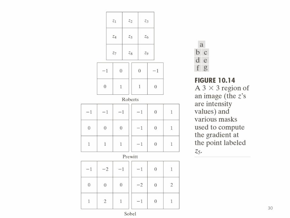
Basic Edge Detection by Using First-Order Derivative
28
2 2
1
( )
The magnitude of
( , ) mag( )
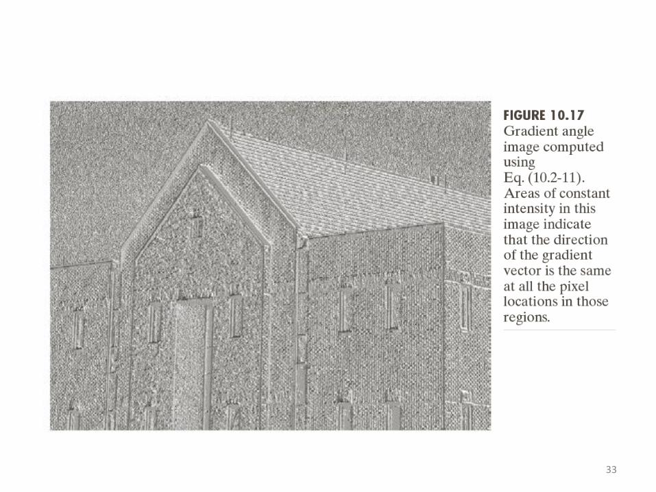
The direction of
( , ) tan
The direction of the edge
-90
x
y
x y
x
y
f
g xf grad f
fg
y
f
M x y f g g
f
gx y
g

Basic Edge Detection by Using First-Order Derivative
29
Edge normal: ( )
Edge unit normal: / mag( )
x
y
f
g xf grad f
fg
y
f f
In practice,sometimes the magnitude is approximated by
mag( )= + or mag( )=max | |,| |f f f f
f fx y x y
30

31
32
33

34
35

36

The Canny Edge Detector
37
►Optimal for step edges corrupted by white noise.
►The Objective
1.Low error rate The edges detected must be as close as possible to the true edge
2.Edge points should be well localized The edges located must be as close as possible to the true edges
3.Single edge point response The number of local maxima around the true edge should be minimum

The Canny Edge Detection: Summary
38
►Smooth the input image with a Gaussian filter
►Compute the gradient magnitude and angle images
►Apply nonmaxima suppression to the gradient magnitude image
►Use double thresholding and connectivity analysis to detect and link edges

39
0.04; 0.10; 4 and a mask of size 25 25L HT T

40 0.05; 0.15; 2 and a mask of size 13 13L HT T

41

42