1Prof. John H. Munro munro5@chass.utoronto.caDepartment of Economics john.munro@utoronto.caUniversity of Toronto http://www.economics.utoronto.ca/munro5/

9 January 2013

ECONOMICS 303Y

The Economic History of Modern Europe to 1914

Prof. John Munro

Lecture Topic No. 15:

III. GREAT BRITAIN AS THE UNCHALLENGED INDUSTRIAL POWER, 1815 - 1873

D. Agriculture in Great Britain: Innovation, Expansion, and Contraction, 1815 - 1914:

D. Agriculture in Great Britain: Innovation, Expansion, and Contraction, 1815 - 1914:

1. Main Trends in 19th-Century British Agriculture:

a) This lecture, commencing the second semester, logically follows from the end of the last semester:

i) i.e., following from the previous two lectures that ended the first semester:

(1) on the transportation revolution: in steam powered railroad and steam shipping, and

(2) on Free Trade: which, in Britain, hinged entirely on the question of agricultural protection.

ii) thus today’s lecture will demonstrate the ultimate, far reaching, and dramatic consequences of both Free Trade and that

transportation revolution:

(1) of the Transportation Revolution: especially in the combined role of railroads and steam shipping in opening up and developing vast new

grain lands for international commerce; and thus

(2) of Free Trade: beginning with the Repeal of the Corn Laws in 1846.

# thus in ultimately permitting a flood of cheap foreign grain imports from the 1860s.

# and those grain imports became all the cheaper as transport costs fell so sharply

iii) the consequence of these two factors combined – the transportation revolution and Free Trade (itself a veritable revolution): was to

bring about a drastic shrinkage of Britain’s agricultural sector, so that only about 7% of the population was engaged in agricultural in 1914, when

this course ends.

iv) The adoption of the Gold Standard was also a vital component of British Free Trade (as seen in the last lecture, on foreign trade in

December).

(1) there could have been no genuine Free Trade without the Gold Standard: to prevent currency manipulations

(2) the international gold standard meant fixed exchange rates between nations on the standard:

# in that the value of each currency was defined as a fixed weight (grams) of pure gold

# as the necessary component of the Gold Standard thus prevented protectionism in the form of exchange rate depreciation or

‘devaluations’

(3) devaluations were frequently used by non-GS countries (then and later) as artificial devices to promote exports and curb imports.

(4) consider this situation in light of the current problems of world trade, and the role of the euro zone.

v) We shall see proof of my arguments about the benefits of Free Trade: when we go to continental Europe to examine the changes in the

post-1860 economies of France, Germany, and Russia:

(1) For all these countries maintained or restored agricultural protection,

(2) in order to prevent a contraction of their agricultural sectors, with a flood of cheap imports.

(3) so that, indeed, their agricultural sectors contracted far less than did the British agricultural sector

(4) consequently their citizens experienced much higher cost food and other agricultural products, and living costs in general”

# because of less productive (more costly) agriculture, their living standards (real incomes) remained lower than the British, up to World

War I

# again, the chief factor in the rise of real incomes in Great Britain after the 1850s was relatively cheaper foodstuffs

vi) Britain’s economic transformation by the Law of Comparative Advantage:

(1) The key message to be understood is this:

# that the combination of the international Transportation Revolutions and Free Trade – more accurately, Free Trade plus the Gold

Standard– together forced the British economy to obey the law of comparative advantage:

# i. e., to contract its agricultural sector: in which it had no such advantage, except in some specialized crops and some aspects of livestock

production,

# and thus: to divert capital, labour, and resources to industry, finance, commerce, and shipping, where the British did enjoy such

advantages in exports,

(2) That allowed Great Britain to acquire its food – and especially grains – far more cheaply through imports that were financed by exporting those

goods and services.

vii) No other country in the world had its economy more dramatically altered

(1) by this combination of the transportation revolution + Free Trade + Gold Standard,

(2) and, consequently, by an agricultural contraction that shifted resources to be used more productively in other sectors of the economy.

viii) Welfare effects: can at least be deduced from the fact that Britain consistently enjoyed the highest real incomes in Europe from the 1870s to

World War I, as I will demonstrate with statistical tables at the end of this lecture – and again in the final lectures of this course.

b) Historical survey of the major changes in British agriculture during the 19th century:

from the Napoleonic Wars in to the outbreak of World War I in 1914,:

i) 1793 - 1815: period of the French Revolutionary and Napoleonic Wars:

(1) very high, inflated grain prices:

# as population pressure mounted forcing England to import more and more grain,

# and as foreign grain supplies were often cut off in time of war.

(2) But grain price increases were partly inflationary, during the era of the ‘paper pound’ (1797-1821, though grain prices began to fall from

1815.)

ii) 1815 - 1846: Post Napoleonic Wars: the Era of the Corn Laws

(1) Marked the completion of the so-called Agricultural Revolution:

# with enclosures, convertible husbandry, multiple course crop rotations, etc.

# but not yet with any significant mechanisation.

(2) grain farmers experienced a mild recession, with falling prices.

(3) As a result of that recession, British farmers clamoured for protection:

# in the form of the Corn Laws [to be analysed separately], which dominated this era,

# until their repeal and the adoption of Free Trade in 1846.

iii) 1846 - 1873: Free Trade and the age of ‘High Farming’

# with an unexpected expansion and general prosperity for most farmers:

# a veritable Golden Age of British Farming, despite fears about Free Trade.

iv) 1873 - 1914: Agricultural Depression:

(1) To repeat with justified emphasis, this finally was the era, but only from the 1870s, when both Free Trade and the Transportation Revolution

brought home bitter fruits for British grain farmers especially, with severely falling prices.

(2) Agriculture experienced a much more pronounced shift to livestock raising;

(3) nevertheless there was still an overall contraction in the agricultural sector: with a fall in its share GDP from about 25% in the 1860s to 7% by

the eve of World War I.

c) Major Features of Agrarian change in summary:

i) first, over the long-run, the predominant feature was a shift away from grain or arable agriculture into livestock raising, essentially reflecting a

shift of relative prices in favour of livestock products;

ii) second, the symbiotic role of agriculture in the Free Trade Movement, and the role of both Free Trade and the Transportation Revolutions

on in changing the agricultural sector

iii) third, from the 1870s, as these two forces hit Britain,

(1) a very radical reduction in the grain-growing sector and then -

(2) an overall contraction in the agricultural sector, by 1914

2. Farming in the Era of the Corn Laws, 1815 - 1846

a) Behaviour of Prices during the Corn Law era: showing some shift in relative prices that further favoured livestock production.

i) the behaviour of grain prices, with the end of the Napoleonic Wars in 1815 (as we saw in the Free Trade lecture, in December):

(1) grain prices plunged almost immediately, right after the wars, with the resumption of normal trade

(2) and then, grain prices fluctuated around a much lower level until the 1830s.

(3) though admittedly at a generally higher level than those for pre-war grain prices.

ii) livestock prices, however, did not fall as much, remained stable, or even rose in some periods.

iii) This shift in relative prices favouring livestock products is a fairly constant trend throughout the 19th century, from the Napoleonic

Wars to World War I, from 1815 to 1914.

iv) Differences in elasticities of demand and supply explain that shift: but especially in demand (price elasticity and income elasticity):

(1) cheaper grain, with inelastic demand, liberated more income to be spent on livestock products (and indeed other non-grain products);

(2) livestock products are more elastic in supply to the agricultural sector than are grain crops;

(3) For it is easier to adjust livestock products for the market, especially with convertible husbandry.

b) Reasons for the Price Slump in Grains after 1815:

i) in part just monetary factors:

(1) with the end of inflationary wartime deficit financing, the end of the paper pound and the return to a gold-backed pound (from 1821),

monetary contraction and deflation quickly set in.

(2) But since grain prices fell more than did the price level, and certainly more than industrial prices, we also have to look at various real factors

also.

ii) real factors:

(1) restoration of grain imports with return to peace: very important since Britain had become a net food importer from the 1770s (and

remained so to this very day).

(2) Expansion and completion of Enclosures: and the related spread of modern farming techniques, sufficient to raise the general level of

agricultural productivity [to be demonstrated later in the lecture].

(3) Then, from the 1830s, the development of the railroad: which had a very significant impact in cutting costs and lowering agrarian prices.

c) Other Cost-Cutting Innovations after 1815:

i) widespread use of guano fertilizers: from Peru (reflecting British trade expansion with South America in the 1820s): bat dung.

ii) introduction of steam-powered agricultural machinery:

(1) the Scottish mechanical thresher:

(2) and steam-powered ploughs, using portable steam-engines

(3) but chiefly only from the 1840s

iii) improved scientific livestock breeding: to increase the size and weight of cattle to increase the amount of meat so produced.

d) Patterns of Agrarian Change:

i) as noted and stressed, a gradual shift away from grain farming into livestock farming

(1) often as part of convertible husbandry or Norfolk four-course rotations, with stall-fed livestock

(2) in response to that shift in relative prices, which, as noted, favoured livestock farming.

(3) see the graph: which shows that livestock product prices were rising in relation to grain prices, from the 1820s, and more markedly so from the

1840s

ii) Cause and effect were also interrelated in agrarian changes:

(1) because the spread of improved farming techniques that reduced costs and thus prices were also undertaken in response to falling grain prices:

(2) i.e., the necessity to cut costs just in order to survive

(3) and/or to shift out of grain into convertible husbandry,

(4) or completely into livestock farming.

e) Barriers to Further Agricultural Changes, 1815 - 1846:

i) Continued population growth accompanied by low and falling agricultural wages: thus curbed the incentive to mechanize agriculture (i.e.

to substitute costly capital for cheap labour).

ii) Lack of capital, or access to sufficient capital, for many farmers:

(1) the new husbandry, with more livestock, required 40% more capital than the traditional three-field system.

(2) and that was true, even without the application of agricultural machinery.

iii) Geography and Adverse soils:

(1) especially the critical problem of water drainage in the eastern Midlands.

(2) heavy, wet clay soils were quite unsuitable for the new husbandry and multiple course rotations; (3) such soils thus restricted local agriculture

to the traditional grain-oriented three-field system.

iv) Agricultural protection under the Corn Laws:

(1) Protective tariffs had sheltered many grain farmers from the necessity of making adjustments. (2) This brings us to the next and important

topic of the Corn Laws

f) The Corn Laws: the bulwark of agricultural protection.

i) Please note once again that the word ‘corn’ in England (and in Europe) means grain in general, or the chief grain of the region, which in

England was wheat.

ii) The English Corn Laws, which went back to the later 17th century, were the bulwark of agricultural protection: they provided

(1) a combination of import tariffs, import prohibitions, and

(2) export bounties (government subsidies to export)

(3) all of which were designed to protect and foster grain English grain growing.

iii) After the Napoleonic Wars, with the immediate post-war slump in grain prices, this protection was sharply increased.

iv) Much land that had been brought under the plough during wartime high prices was now uneconomic for grain farming,

v) so that British farmers demanded complete protection, i.e., against imported foreign grains.

vi) The Corn Law of 1815: was thus enacted in response to the sharp fall in post-war grain prices.

(1) This law prohibited wheat imports unless prices rose above the war time average of 80 shillings (s.) = £4 sterling, a ‘quarter’ (a grain measure

= 8 bushels or 64 gallons).

(2) But this 1815 Corn Law proved almost impossible to enforce.

(3) Thus forcing a major amendment in the Corn Laws, in:

vii) The Corn Law of 1828:

(1) it substituted a sliding scale of import duties, in place of import prohibitions: i.e., the lower the market price for grain, the higher would be the

duties imposed

(2) with no duties imposed when prices rose higher than 73s. a quarter.

(3) The object was to make it expensive to import grain during normal times, but to permit grain imports during times of high or famine prices.

viii) 1839: formation of the Anti-Corn Law League in Manchester:

(1) in the midst of a severe industrial depression, from 1836 to 1842

(2) which I have mentioned several times now: an era bad harvests, high prices, and high unemployment.

ix) Harvest and Famine Crises of 1846: Drastic harvest failures in northern Europe, with famine grain prices and a severe economic crisis

(which we saw with the Bank of England).

x) The result:

(1) was the Repeal of the Corn Laws, as we saw in more detail in the previous topic on Free Trade (in December), by, ironically, the Tory

(Conservative) government of Robert Peel.

(2) Remember from the last lecture that the Conservatives had long championed the Corn Laws, to secure support from the mass of rural voters,

from land owners to tenants

(3) That Repeal of the Corn Laws thus meant the complete removal of agricultural protection.

3. The Golden Age of British Farming: ‘High Farming’, 1846 - 1873

a) The Consequences of Repealing the Corn Laws in 1846:

i) contrary to what so many farmers had feared or expected, the results were by no means disastrous:

(1) true, grain imports did increase: in fact, in proportional terms, they more than doubled (Table 11),

# from feeding 8.2% of the population in 1831-40 (1.4 million)

# to feeding 18.4% of the population in 1841-50 (3.6 million)

(2) and grain prices did fall somewhat,

# but only by about 5s. a quarter

# or less, as the table on screen (and in the appendix)shows

(3) Then in the 1850s and 1860s, grain prices (including potato prices) collectively actually rose somewhat (graph).

ii) Disaster for grain farmers would indeed come later,

(1) but only twenty or more years later:

(2) in the interim, British grain farmers were still partly protected by high transportation costs

# or what was rightly called the ‘tariff of bad roads’

# i.e., high shipping costs, before the onset of the revolution in steam-powered maritime transport.

iii) Furthermore, the entire agricultural sector benefited from a general economic boom:

(1) This was a European-wide economic boom, for the mid century decades.

(2) As we saw in the previous lecture on Free Trade (in December):

# from the late 1840s to the early 1870s, Britain especially, but also most West European countries,

# experienced a tremendous boom in international trade, in exports and imports combined, obviously.

iv) The Livestock and other non-grain sectors benefited especially:

(1) thus while wheat and some other grain prices did fall gently,

(2) prices for livestock, dairy products, fruits and vegetables, industrial crops, etc., generally rose fairly sharply over this period (in both nominal

and real terms), as the graph shows.

b) Factors Promoting Agricultural Prosperity:

i) Considerable growth in urbanization:

(1) with industrialization and the railroad.

(2) Thus larger, more concentrated markets for foodstuffs.

(3) Remember the obvious point: urban dwellers do not produce their own food, which they must purchase from sources outside the city: either

rural hinterlands or imports

ii) Effect of the railroad, as noted before,

(1) in bringing all agrarian areas within the market economy, and

(2) especially in improving markets for livestock and dairy products and

(3) in creating new urban markets for perishable fruits and vegetables.

iii) Rising Living Standards: Engels Law, Inferior Goods, and Giffen Goods

(1) both pessimists (Marxists) and optimists (Conservatives) seem to be in agreement that, from the later 1840s, the real wages and living

standards of the working classes (of almost everybody) were now, finally, rising – and rising strongly.

(2) Engels Law: The significance of rising real incomes for agriculture can be seen in Engels Law, concerning the income elasticity of demand:

i.e.,

# with rising real incomes, proportionately less of an average family’s real income is spent on bread or cheap carbohydrates (inferior goods)

and thus

# proportionately more of that average family’s disposable income is spent on meat, dairy products, fruits and vegetables, etc.

(3) The Economic Significance of Inferior goods:

# goods for which demand falls when their prices fall or when real incomes rise;

# and vice versa: demand rises when their prices rise, or real incomes fall

(4) The Economic Significance of Giffen Goods

# A Giffen Good is a special case of an Inferior Good

# This term is named after Sir Robert Giffen ‘to whom Alfred Marshall attributed the observation that, among the labouring classes, when

the price of bread (the main item of their diet) rose, their consumption rose; and when its price fell, their consumption also fell’.1

# and a rise in his real income will conversely lead to a relative decline in the consumption of the inferior good (bread).

# In the case of a Giffen good, a rise in its price will cause a rise in its (relative) consumption; and a fall in its price will similarly cause a

relative fall in its consumption.

# Thus apparently contradicting the basic ‘law of demand’: namely, that demand, i.e., the quantity demanded, varies inversely with the

price.

# For this to be true (that demand varies directly with the price), the income effect must outweigh the substitution effect.

# i.e., expenditures on bread represent a large proportion of a labourer’s real income,

! so that a rise in its price has an important effect in reducing his real income, ceteris paribus, forcing a reduction in his

expenditures on other more expensive foodstuffs,

1 Graham Bannock, R.E.Baxter, R. Rees, The Penguin Dictionary of Economics, 3rd edn (London, 1984), pp. 190-91.

! thus also forcing him to consume more bread in their place, so long as there are no other cheaper foodstuffs (with the same

nutritional value) that can be substituted for the bread.2

(4) The overall significance of the combined fall in the real price of bread grains and in rising real incomes (especially for the working

classes): Thus a significant force in providing growing prosperity for these non-grain sectors of agriculture.

4. Technological Change in the Age of High Farming, 1846 - 1873

a) British agriculture underwent significant technological changes from the 1840s

i) The two most important features were:

(1) mechanization: with steam powered-machinery

(2) the resort to chemical fertilizers

ii) These two aspects were interrelated: especially in terms of the impact of mechanization upon the supplies of livestock for draught animals

and on the fodder crops to feed them

b) Greater Mechanization of Agriculture during ‘Age of High Farming’: steam-powered machinery

i) key incentive to mechanize lay in the increasing scarcity of agricultural labourers : and the 1840s marks the first time that the absolute

numbers of agricultural workers actually fell.

(1) From the 1840s to the 1870s, their numbers fell by 22%.

(2) Evidence indicates that this fall, the drift of labour away from the land, preceded any significant mechanization;

(3) and so mechanization should not be seen as the cause of the fall in labour supply, of labour displacement.

ii) Factors producing an outflow of labour from agriculture:

(1) railroad construction from the 1830s: drew heavily on rural labour.

(2) labour mobility that railroads provided: moving people to the towns.

(3) increased steam-powered urban industrialization, certainly with a decisive shift of textile manufacturing from rural to urban areas,

2 Ibid., p. 191: ‘The overall change in the quantity of the good demanded following a change in its price is the resultant of these two effects: the income effect and the substitution effect. If the income effect works so as to change the demand in the same direction as the price change (i.e., the good is an inferior good), while the substitution effect works so as to change demand in the opposite direction to the price change (always the case), and if the former effect outweighs the latter, the net effect is that the quantity demanded changes in the same direction as price. It was this special case which was observed by Giffen.’

(4) especially when most industries were offering much higher wages than agriculture.

iii) Examples of Steam-Mechanization in British Agriculture:

(1) increased use of the aforementioned steam-powered ploughs

(2) steam powered Scottish threshers (which first came into use during the 1820s).

(3) from the 1850s, the American mechanical reaper: the McCormack Reaper.

(4) Also: mechanical, steam-powered harvesters, binders, separators.

c) The Drainage of the Midland Clay Soils: from the 1840s

i) invention of drain-tile making machines in the 1840s: an aspect of mechanization

(1) i.e., clay pipes for water drainage.

(2) Steam pumps and mass produced drain tiles cut drainage costs by up to 40%.

ii) Government Assistance, in 1846: British government offered low cost, subsidized loans for drainage in the East Midlands.

iii) Such drainage schemes offered possibility of converting these heavy wet clay soils (alluvial) from three-field rotations to convertible

husbandry or to Norfolk Farming (multiple rotations without fallow), with much higher yields.

iv) Reality, however, did not match such hopes:

(1) it has been estimated that by the 1880s only about 20% of the clay soils had been adequately drained;

(2) and at a very high costs, which largely reflected mis-investment.

d) Comparisons of Mechanization in European and North American agriculture

i) in Europe: not surprisingly, British agriculture, by 1900, came to be much more mechanized than continental European agriculture, with the

exception of some parts of eastern Germany.

ii) but in North America, especially the US, the contrary was true: By

(1) by the later 19th century, early 20th century, American agriculture was, also not surprisingly, much more extensively mechanized than

was the British:

(2) in 1910, American agriculture was about 80% mechanized, while British agriculture was only about 50% mechanized.

iii) Differing factors: to explain the relative extent of mechanization in U.S. vs. Great Britain

(1) Higher wages in U.S. farms: more incentive to mechanize, i.e., to substitute capital for labour

(2) Capital was more readily accessible to U.S. farmers.

(3) farming scale was much larger in the U.S. than in Britain:

# large scale necessary to justify application of machinery

# though many small British farms rented portable and itinerant steam engines

(4) Terrain was also much flatter in much of the U.S, especially the major grain-growing areas of the Great Plains: and thus such terrain was much

less injurious to machinery.

e) The Impact of Mechanization on Livestock Husbandry, Food Supplies, and Fertilizers.

i) First, Mechanization and the Food Supply: contributions to productivity and growth

(1) First, obviously, these machines, in displacing labour, vastly increased labour productivity (and indirectly land productivity).

(2) thus significantly increasing output at falling marginal costs.

ii) increased efficiency of capital:

(1) in that farm machines were displacing not only labour, but other forms of capital,

(2) especially capital in the form of draft animals: horses and oxen principally

iii) The impact on livestock husbandry: draught animals

(1) in doing so, agricultural machinery thus machines significantly economized on arable food production:

# i.e., foodstuffs that otherwise would have been used as fodder crops to feed these animals.

# According to one economic historian, for example, in the US, in the 1920s, even with extensive mechanization, but before complete

mechanization, draft animals were still consuming about 25% of total arable outputs.3

iii) However, the pronounced shift, especially in British agriculture during the late nineteenth-century into livestock-oriented agriculture

necessarily entailed:

3 See D. Gale Johnson, review for EH.Net (28 November 2001), of: Vaclav Smil, Enriching the Earth: Fritz Haber, Carl Bosch, and the Transformation of World Food Production (Cambridge, MA: MIT Press, 2001). xxii + 338 pp. $34.95 (hardcover), ISBN: 0-262-19449-x. [D. Gale Johnson, Professor of Economics, Emeritus, University of Chicago. <j015@midway.uchicago.edu>]In his review, Johnson states that : ‘What Crookes did not foresee, and what Smil does not recognize, was the role the tractor played in contributing to the food supply, especially in the industrial nations, after World War I. It was estimated that draft animals utilized a quarter of all the harvested output of American agriculture in the 1920s (Gray, 1924). In fact, researchers in the United States Department of Agriculture wrote a long article in the early 1920s in which they indicated that the United States would have to reduce its consumption of animal products in order to feed a population of 150 million (Gray, 1924)’.

# a related shift in arable production to the cultivation of those fodder crops (other than grasses and hay) for feeding non-draft farm animals:

# i.e., cattle and sheep, for meat, milk, butter, cheese, and industrial products.

iv) but consider also the impact from the displacement of draft animals: the fertilizer problem

(1) as just noted, that would have meant a some shift or switch in agricultural production from fodder crops, for feeding livestock, to other arable

crops, for human consumption (grains, vegetables), or for industrial uses.

(2) but since so many fodder crops had been nitrogen-fixing legumes, that switch would thus have necessarily diminished the addition of nitrogen

to the soils, from growing those fodder crops

v) the manure problem: furthermore the reduction in the use of draft animals also meant a reduction in the quantity of animal manure available

for fertilizing the soils.

iv) thus the next and obvious question: what further technological changes occurred to remedy this potential deficiency in natural nitrogen

production, for fertilizing the soil?

f) Chemical Fertilizers: provided the solution in what was the key advance of this era.

i) This was much more of a German than a British innovation: the application of synthetic or chemical fertilizers as opposed to natural.

ii) The German chemist Justus von Liebig was the father of modern agricultural chemistry: (1) In 1840, he published [originally, of course,

in German]: Chemistry and Its Application to Agriculture;

(2) and as we shall see later under German agriculture, the Germans quickly took the lead in this field, advancing beyond the British.

iii) The British, however, if behind the Germans, were certainly much ahead of the French:

(1) 1838: foundation of the Royal Agricultural Society.

(2) 1843: establishment of the Rothamstead Experimental Station: important for promoting the use of more productive seeds, better crop rotations,

selective livestock breeding, fertilizers, disease control.

(3) J. B. Lawes: British scientist who discovered a very important, powerful fertilizer called superphosphates: by applying sulphuric acid (H 2SO4)

to animal bones.

g) Overall results of productivity changes in British agriculture: it has been estimated that from the 1830s to 1870s crop yields improved by

50%.

h) The following statistics demonstrate not only the productivity gains in British agriculture, but provide a useful comparison with the

agrarian sectors of the other countries we will be examining:

Indices of European and American Agricultural ProductivityFrom 1810 to 1910

Annual net output per agricultural worker (male)measured in million of calories

COUNTRY 1810 1840 1860 1880 1900 1910

Britain 14.0 17.5 20.0 23.5 22.5 23.5

France 7.0 11.5 14.5 14.0 15.5 17.0

Germany 7.5 10.5 14.5 22.0 25.0

Russia 7.0 7.5 7.0 9.0 11.0

U.S.A 21.5 22.5 29.0 31.0 42.0

Source: Paul Bairoch, ‘Niveaux de développement économique de 1810 à 1910,’ Annales: Économies, sociétés, civilisations, 20 (1965), 1096, Table 1.

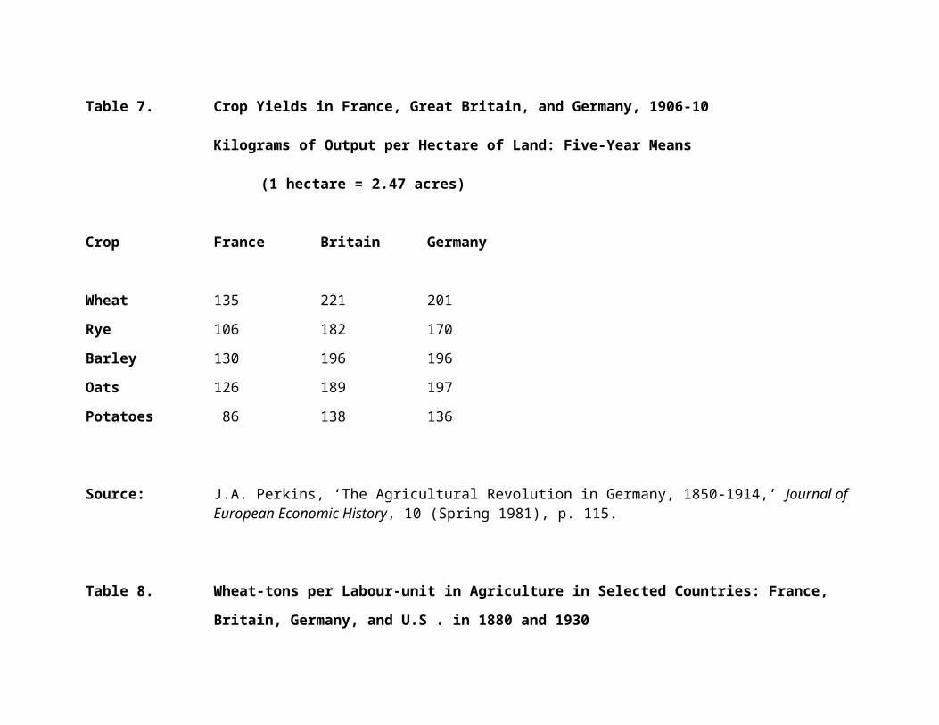
Crop Yields in France, Britain, and Germany, 1906-10

Kilograms of Output per Hectare of Land: Five-Year Means

(1 hectare = 2.47 acres)

Crop France Britain Germany

Wheat 135 221 201

Crop France Britain Germany

Rye 106 182 170

Barley 130 196 196

Oats 126 189 197

Potatoes 86 138 136

Source: J.A. Perkins, ‘The Agricultural Revolution in Germany, 1850-1914,’ Journal of European Economic History, 10 (Spring 1981), p. 115.

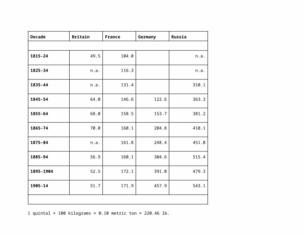
Output of Principal Grain Crops of Selected European Countries, in millionsof quintals, in decennial averages, 1871-90 to 1905-14

Decade Britain France Germany Russia

1781-90 35.0 85.3

1800-13 43.0 94.5 268.6

1815-24 49.5 104.0 n.a.

1825-34 n.a. 116.3 n.a.

Decade Britain France Germany Russia

1835-44 n.a. 131.4 310.1

1845-54 64.0 146.6 122.6 363.3

1855-64 68.0 158.5 153.7 381.2

1865-74 70.0 160.1 204.8 410.1

1875-84 n.a. 161.8 248.4 451.0

1885-94 56.9 160.1 304.6 515.4

1895-1904 52.5 172.1 391.0 479.3

1905-14 51.7 171.9 457.9 543.1

1 quintal = 100 kilograms = 0.10 metric ton = 220.46 lb.

Source: Carlo Cipolla, ed., Fontana Economic History of Europe, Vol. IV:2, pp. 752-53.

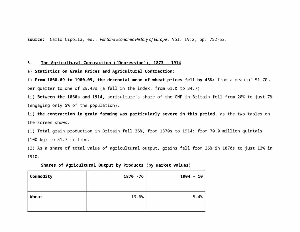
5. The Agricultural Contraction (‘Depression’), 1873 - 1914

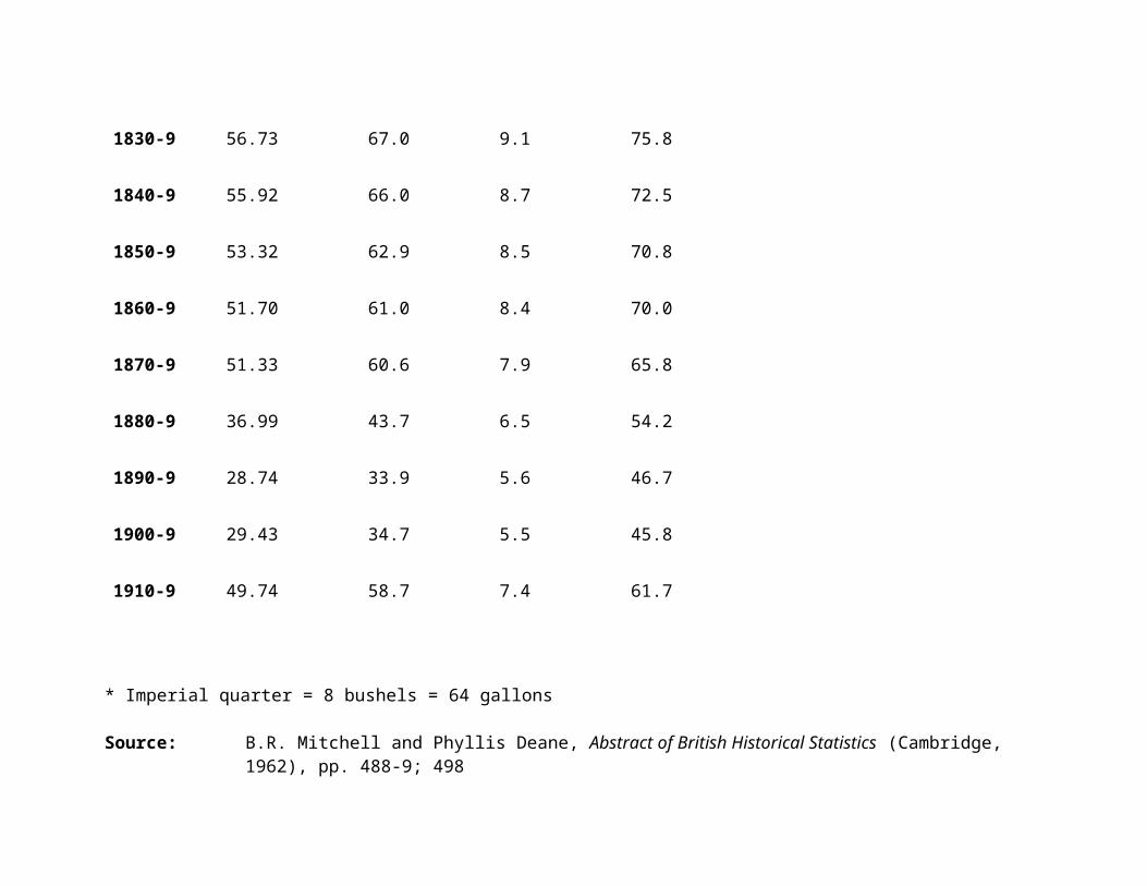
a) Statistics on Grain Prices and Agricultural Contraction:

i) From 1860-69 to 1900-09, the decennial mean of wheat prices fell by 43%: from a mean of 51.70s per quarter to one of 29.43s (a fall in the

index, from 61.0 to 34.7)

ii) Between the 1860s and 1914, agriculture's share of the GNP in Britain fell from 20% to just 7% (engaging only 5% of the population).

ii) the contraction in grain farming was particularly severe in this period, as the two tables on the screen shows.

(1) Total grain production in Britain fell 26%, from 1870s to 1914: from 70.0 million quintals (100 kg) to 51.7 million.

(2) As a share of total value of agricultural output, grains fell from 26% in 1870s to just 13% in 1910:

Shares of Agricultural Output by Products (by market values)

Commodity 1870 -76 1904 - 10

Wheat 13.6% 5.4%

All Grains 25.5% 13.0%

All Arable Crops 41.4% 28.5%

Animal Products 58.6% 71.5%

Total Agricultural Output 100.0% 100.0%

b) Chief reason for this agricultural contraction: was, to repeat (for about the tenth time, now), the combination of the world-wide steam

powered transportation revolution and Free Trade

i) see the graph on the screen (figure 4): for the dramatic drop in trans-Atlantic transport costs in the grain trade:

(1) the rapid decline had begun in the 1860s (though having risen because of the US Civil War)

(2) and then those costs rose briefly in the late 1860s and early 1870s –

(3) insurance and transaction costs also figure into these rates: reflecting European wars

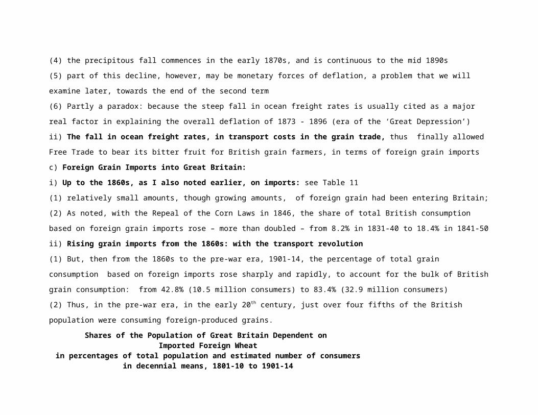
(4) the precipitous fall commences in the early 1870s, and is continuous to the mid 1890s

(5) part of this decline, however, may be monetary forces of deflation, a problem that we will examine later, towards the end of the second term

(6) Partly a paradox: because the steep fall in ocean freight rates is usually cited as a major real factor in explaining the overall deflation of 1873 -

1896 (era of the ‘Great Depression’)

ii) The fall in ocean freight rates, in transport costs in the grain trade, thus finally allowed Free Trade to bear its bitter fruit for British grain

farmers, in terms of foreign grain imports

c) Foreign Grain Imports into Great Britain:

i) Up to the 1860s, as I also noted earlier, on imports: see Table 11

(1) relatively small amounts, though growing amounts, of foreign grain had been entering Britain;

(2) As noted, with the Repeal of the Corn Laws in 1846, the share of total British consumption based on foreign grain imports rose – more than

doubled – from 8.2% in 1831-40 to 18.4% in 1841-50

ii) Rising grain imports from the 1860s: with the transport revolution

(1) But, then from the 1860s to the pre-war era, 1901-14, the percentage of total grain consumption based on foreign imports rose sharply and

rapidly, to account for the bulk of British grain consumption: from 42.8% (10.5 million consumers) to 83.4% (32.9 million consumers)

(2) Thus, in the pre-war era, in the early 20th century, just over four fifths of the British population were consuming foreign-produced grains.

Shares of the Population of Great Britain Dependent on Imported Foreign Wheat

in percentages of total population and estimated number of consumersin decennial means, 1801-10 to 1901-14

Decade Percentage of Total Population

Estimated Number of Consumers of Foreign Wheat

in millions

1801-10 7.0 0.8

1811-20 5.5 0.7

1821-30 4.9 0.7

1831-40 8.2 1.4

1841-50 18.4 3.6

1851-60 28.8 6.3

1861-70 42.8 10.5

1871-80 60.0 16.6

1881-90 70.0 21.9

1891-00 76.5 26.7

1901-14 83.4 32.9

Source:

Mette Enrnæs, Karl Gunnar Persson, and Søren Rich, ‘Feeding the British: Convergence and Market Efficiency in the Nineteenth-Century Grain Trade’, The Economic History Review, 2nd ser., 61: No. S1 (August 2008): Special Issue: Feeding the Masses, ed. Steve Hindle and Jane Humphries, pp. 140-71.

iii) sources of foreign grains: see Table 10, in the Appendix

(1) from the 1870s to the 1890s,

# the predominant source of that grain was the United States, accounting for just under half (43.3% to 47.8%)

# the next most important source was Russia: with about 20% of total imports

(2) from the 1890s to World War I, the US share fell by half (to 23.8%), and the Russian share fell to 14.5%, with the growth of

imports from newer sources: Canada, Argentina, India, Australia-New Zealand.

iv) Thus, as noted, high transportation costs had continued to provide some protection to British grain farmers, up to the

1860s,

v) at the same time, the rapid growth of European population and industrial urbanization had been consuming most of the increased

European supplies.

vi) But finally, as stressed before, the combination of railroads and steam shipping together: opened up vast new grain-growing

lands in Ukraine and S.E. Europe, in Canada and the U.S., in Australia, South America (Argentina), and also India – as the table

shows..

vii) Cheap sea transport allowed a growing flood of that new grain to pour into Britain and Europe, with the consequent

plummeting of grain prices so evident in the table.

viii) Note also the effects of the operation of the international gold standard:

(1) when all major currencies were tied to and evaluated into gold, they were therefore freely convertible into each other and into gold,

(2) the gold standard thus meant an automatic transmission of price changes to the British economy without any deviations.

(3) and, as noted, gold-standard countries could not protect themselves against imports by engaging in currency depreciation (i.e., to

make imports more expensive).

c) Consequences:

i) That problem was the most severe in Great Britain because of her Free Trade policies, which, as we have seen in the previous

lecture (in December), were rigidly maintained up until World War I.

ii) In Britain, the consumption of home-grown wheat: fell from 61% of the total in 1860s to just 27% (27.1%, to be more exact) in

1900.

iii) But on the continent, as we shall see later, most countries reacted to the agricultural slump by restoring agricultural tariffs;

and with that protection their grain-farming sectors did not contract as much.

iv) In Britain, the other non-grain sectors, especially livestock, also did not contract as much, because

(1) international competition in those areas was not so severe.

(2) relative prices for these products remained much more favourable than prices for grains, etc.

iv) Thus these forces completed the shift away from grain into livestock and dairy farming: and what survived of British

agriculture was and remained very highly efficient.

v) Though British grain farmers suffered, Britain as a whole benefited greatly from these changes: benefited from the law of

comparative advantage, the gains of trade, with much cheaper food.

(1) It was far cheaper for Britain to import foodstuffs exchanged for manufactured goods and services than it was for Britain to

produce all of her food at home.

(2) But the food produced at home in the now small surviving agricultural sector was very efficiently produced at low cost, in an

agriculture now strongly devoted to livestock, dairying, and truck farming (fruits and vegetables).

vi) Population Growth, Economic Growth, and Trade: Grain Imports

(1) note, and remember, that the population of Great Britain (Table 10) more than tripled in the 19th and early 20th centuries:

# from about 12 million, in 1810, just before end of the Napoleonic Wars in 1815

# to about 41 million in 1910, before the outbreak of World War I (in 1914)

# In England and Wales: from 10.563 million in 1811 to 36.136 million in 1911

(2) Thus the importance of these economic developments and Free Trade: for there is absolutely no way that England and Wales (or

Great Britain) could possibly have fed itself from its own agrarian resources.

(3) Thus Britain could only have done so, fed that rapidly growing and very large population, through industrialization and foreign

trade: by exporting industrial and various shipping and financial services in order to import those necessary foodstuffs, and to do so

cheaply.

(4) Cheap food imports were thus the consequence of:

# the aforesaid transportation revolution

# Free Trade, combined with the Gold Standard (to prevent currency value fluctuations)

# rapid growth of the industrial, commercial, and financial sectors

(5) Note from Table 12 that, while Britain’s population almost quadrupled from 1800, no other Western European country came close

to that demographic increase.

(6) While Russia’s demographic growth did match the British, the consequences were entirely different, for reasons that we shall see

next term.

vii) Note the importance of foodstuffs for the cost of living and thus the standard of living of much of British society: especially

for the working and lower-middle classes

(1) For centuries and up to the very late 19th century, the combination of food and drink together – grains, meats, dairy products, beer,

etc – accounted for as much as 80% of typical household expenditures.4

(2) In the 1890s, as much as 25% of British working class male expenditures went on drink, principally beer & ale, but also gin.

(3) Currently in Canada (2009 data), food and drink together account for just 20% of household expenditures: see Table 15 in the

Appendix

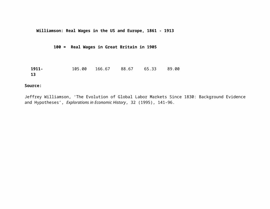
viii) The impact of cheap imported foodstuffs on the British standard of living can best be appreciated from the following

tables (which I will show again, at the end of this course) – and the real-wage graph for England, on the screen:

4 See E.H. Phelps Brown and Sheila V. Hopkins, ‘Seven Centuries of the Prices of Consumables, Compared with Builders’ Wage Rates’, Economica, 23:92 (November 1956), 296-314; reprinted in E.M. Carus-Wilson, ed., Essays in Economic History, 3 vols. (London, 1954-62), vol. II, pp. 179-96, and in E.H. Phelps Brown and Sheila V. Hopkins, A Perspective of Wages and Prices (London: Methuen, 1981), pp. 13-59, containing additional statistical appendices not provided in the original publication, or in earlier reprints. See also John Munro, ‘Builders’ Wages in Southern England and the Southern Low Countries, 1346 -1500: A Comparative Study of Trends in and Levels of Real Incomes’, in Simonetta Cavaciocchi, ed., L’Edilizia prima della rivoluzione industriale, secoli XIII-XVIII, Atti delle “Settimana di Studi” e altri convegni, no. 36, Istituto Internazionale di Storia Economica “Francesco Datini” (Florence: Le Monnier, 2005), pp. 1013-76, on the construction of Consumer Price and Real Wage indices.

Williamson: Real Wages in the US and Europe, 1861 - 1913

100 = Real Wages in Great Britain in 1905

Years Great Britain

U.S. Belgium France Germany

1861-65 61.20 87.60 50.80 45.00 56.20

1866-70 63.20 100.40 56.60 48.20 55.40

1871-75 74.00 120.60 66.00 50.60 61.60

1876-80 83.60 115.60 64.60 54.80 63.80

1881-85 88.00 129.60 71.00 59.60 66.60

1886-90 95.40 139.80 79.80 62.60 73.20

1891-95 100.00 145.00 83.00 63.60 75.60

1896-00 104.80 152.00 89.40 67.60 82.20

1901-05 100.40 163.00 85.80 71.60 83.40

1906-10 107.40 170.20 86.00 74.80 87.00

1911-13 105.00 166.67 88.67 65.33 89.00

Source:

Jeffrey Williamson, ‘The Evolution of Global Labor Markets Since 1830: Background Evidence and Hypotheses’, Explorations in Economic History, 32 (1995), 141-96.

Indices of Relative GDP per capita, compared to US GDP per capita (1.000)for each year of the series

Country 1820 1830 1840 1850 1860 1870 1880 1890 1900 1913 1929 1938

United Kingdom

0.965 1.004 0.975 1.000 0.971 1.004 0.903 0.915 0.917 0.847 0.774 0.898

France 0.713 0.784 0.790 0.781 0.821 0.809 0.753 0.784 0.768 0.770 0.605 0.623

Nether-lands

0.800 0.768 0.814 0.791 0.766 0.787 0.708 0.735 0.715 0.668 0.594 0.704

Belgium 0.749 0.742 0.792 0.836 0.793 0.791 0.772 0.743 0.560 0.698

Germany 0.609 0.681 0.679 0.620 0.738 0.753 0.742 0.607 0.811

Austria 0.551 0.554 0.541 0.518 0.575 0.523 0.543 0.531 0.532 0.504 0.570

Denmark 0.513 0.584 0.616 0.661 0.626 0.659 0.618 0.644 0.668 0.667 0.662 0.741

Switzerland 0.687 0.726 0.741 0.726 0.674 0.761

Italy 0.641 0.589 0.535 0.525 0.512 0.526 0.472 0.529

Spain 0.638 0.638 0.554 0.564 0.567 0.521 0.511 0.463 0.331

Russia 0.410 0.445 0.452 0.451

Australia 1.022 1.174 1.370 1.096 1.304 1.130 1.049 1.085 0.976 0.976 0.860 0.924

Canada 0.827 0.834 0.828 0.740 0.809 0.853 0.968 0.900 0.914

Japan 0.265 0.307 0.335 0.375 0.412 0.440

Argentina 0.734 0.782 0.762 0.813 0.648 0.558

Source: Leandro Prados de la Escosura, ‘International Comparisons of Real Product, 1820 - 1990: An Alternative Data Set’, Explorations in Economic History, 37:1 (January 2000), 1-41.

Table 1. UNITED KINGDOM: GRAIN PRICESDecennial Means of Wheat Prices in the United Kingdom

and of Bread Prices in London, 1770/79 to 1910/9Mean of Prices for 1800-09 = 100

Year Wheat Prices Bread Prices

Shillings Index: pence per Index:

per 1800-9 = loaf of 1800-9 =

Quarter* 100 4 lb 100

1770-9 46.85 55.3 6.5 54.2

1780-9 46.12 54.4 6.4 53.3

1790-9 57.62 68.0 7.7 64.2

1800-9 84.71 100.0 12.0 100.0

1810-9 91.40 107.9 13.6 113.3

1820-9 59.81 70.6 9.9 82.5

1830-9 56.73 67.0 9.1 75.8

1840-9 55.92 66.0 8.7 72.5

1850-9 53.32 62.9 8.5 70.8

1860-9 51.70 61.0 8.4 70.0

1870-9 51.33 60.6 7.9 65.8

1880-9 36.99 43.7 6.5 54.2

1890-9 28.74 33.9 5.6 46.7

1900-9 29.43 34.7 5.5 45.8

1910-9 49.74 58.7 7.4 61.7

* Imperial quarter = 8 bushels = 64 gallons

Source: B.R. Mitchell and Phyllis Deane, Abstract of British Historical Statistics (Cambridge, 1962), pp. 488-9; 498

Table 2. BRITISH AGRICULTURAL STATISTICS

Indices of Output, Prices, and Incomes, 1860 - 1910

Mean of 1860 = 100

Year Agricultural Agricultural Agricultural Agri. RealOutput Prices Population Incomes

1860 100 100 100 100

1870 105 102 89 116

1880 100 91 79 120

1890 106 76 75 130

1900 97 73 69 127

1910 103 83 72 136

Table 3. Percentage Changes in Total Factor Productivity:

Average Annual Rates

From 1790 to 1815 +0.2% per annum growth

From 1816 to 1846 +0.3% per annum growth

From 1847 to 1870 +0.5% per annum growth

....................................................................

Table 4. Value of Agricultural Output as a Share of the British GNP

1860 20% of GNP

1914 7% of GNP

Table 5. Shares of British Agricultural Output by Products

1870 - 76 1904 - 10

Wheat 13.6% 5.4%

All Grains 25.5% 13.0%

All Arable Crops 41.4% 28.5%

Animal Products 58.6% 71.5%

Total Agricultural Output 100.0% 100.0%

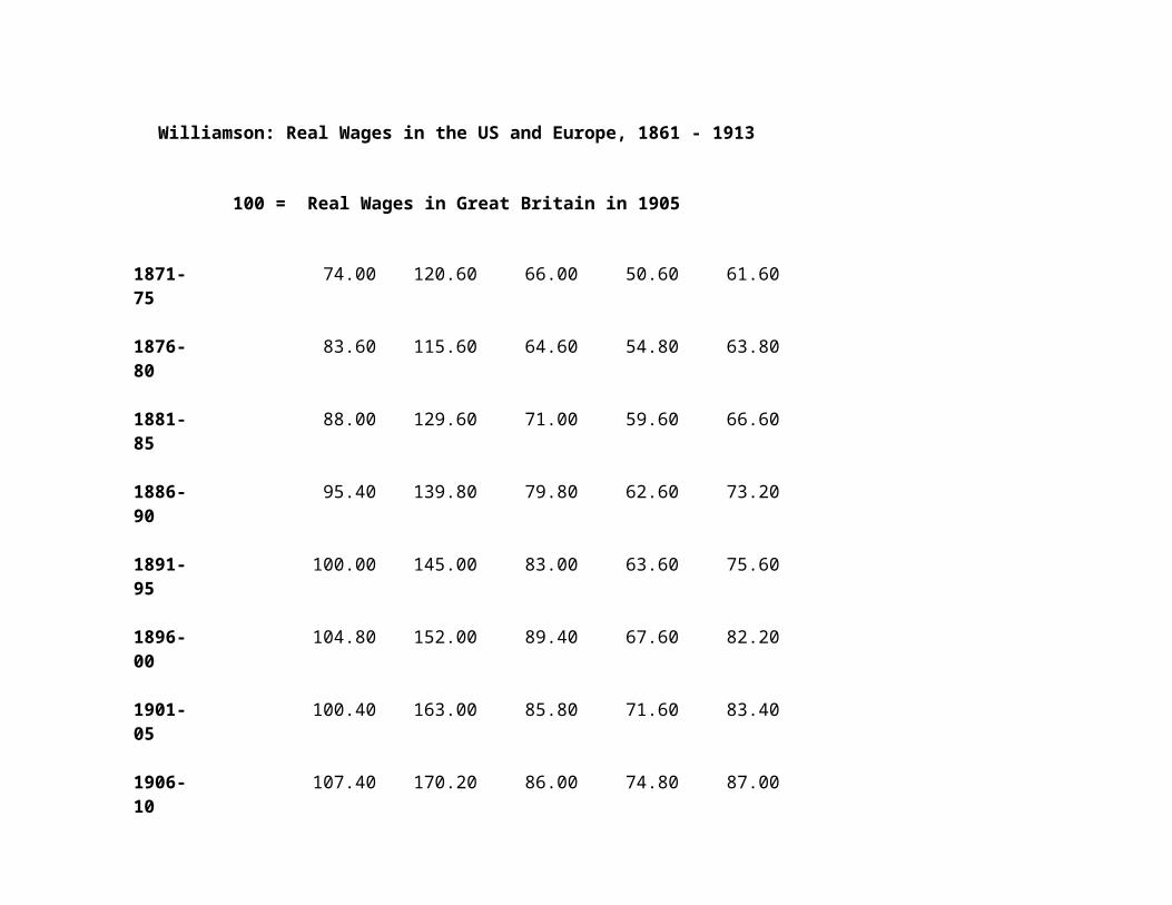
Table 6. Output of Principal Grain Crops of Selected European Countries, in millions

of quintals, in decennial averages, 1871-90 to 1905-14

GreatDecade Britain France Germany Russia

1781-90 35.0 85.3

1800-13 43.0 94.5 268.6

1815-24 49.5 104.0 n.a.

1825-34 n.a. 116.3 n.a.

1835-44 n.a. 131.4 310.1

1845-54 64.0 146.6 122.6 363.3

1855-64 68.0 158.5 153.7 381.2

1865-74 70.0 160.1 204.8 410.1

1875-84 n.a. 161.8 248.4 451.0

1885-94 56.9 160.1 304.6 515.4

1895-1904 52.5 172.1 391.0 479.3

1905-14 51.7 171.9 457.9 543.1

1 quintal = 100 kilograms = 0.10 metric ton = 220.46 lb.

Source: Carlo Cipolla, ed., Fontana Economic History of Europe, Vol. IV:2, pp. 752-53.

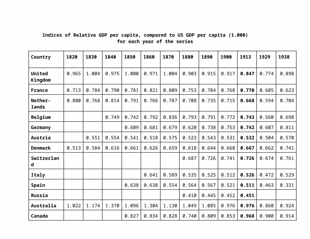
Table 7. Crop Yields in France, Great Britain, and Germany, 1906-10

Kilograms of Output per Hectare of Land: Five-Year Means

(1 hectare = 2.47 acres)

Crop France Britain Germany

Wheat 135 221 201

Rye 106 182 170

Barley 130 196 196

Oats 126 189 197

Potatoes 86 138 136

Source: J.A. Perkins, ‘The Agricultural Revolution in Germany, 1850-1914,’ Journal of European Economic History, 10 (Spring 1981), p. 115.

Table 8. Wheat-tons per Labour-unit in Agriculture in Selected Countries: France, Britain, Germany, and U.S . in

1880 and 1930

Country 1880 1930

France 7.4 13.2

Great Britain 16.2 20.1

Germany 7.9 16.0

United States 13.0 22.5

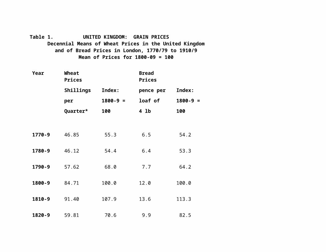
Table 9.

Indices of European and American Agricultural Productivity

from 1810 to 1910

Annual net output per agricultural worker (male)measured in million of calories

COUNTRY 1810 1840 1860 1880 1900 1910

Britain 14.0 17.5 20.0 23.5 22.5 23.5

France 7.0 11.5 14.5 14.0 15.5 17.0

Germany 7.5 10.5 14.5 22.0 25.0

Russia 7.0 7.5 7.0 9.0 11.0

U.S.A 21.5 22.5 29.0 31.0 42.0

Source: Paul Bairoch, ‘Niveaux de développement économique de 1810 à 1910,’ Annales: Économies, sociétés, civilisations, 20 (1965), 1096, Table 1.

Table 10.

Wheat Imports into the United Kingdom by Exporting Nations, 1831-40 to 1901-1914in percentages of total imports

Decade Germany France Russia Canada U.S. Argentina India Australia NZ

Denmark

1831-40 32.0 11.8 13.3 4.5 1.9 n.a. n.a n.a. 3.9

1841-50 40.3 9.8 15.1 1.8 4.2 n.a. 0.0 0.4 3.5

1851-60 26.1 8.9 18.4 1.6 15.5 n.a.. 0.0 n.a 6.2

1861-70 20.5 3.2 26.9 5.5 27.2 n.a. 0.0 0.4 2.0

1871-80 7.4 1.6 20.4 6.8 47.8 n.a. 3.9 3.3 0.7

1881-90 3.5 n.a. 20.2 3.7 43.3 2.1 16.2 4.8 0.1

1891-00 1.2 n.a. 16.8 5.9 45.8 11.5 9.7 3.2 0.0

1901-14 n.a. n.a. 14.5 15.1 23.8 17.5 16.4 9.5 0.0

Source:

Mette Enrnæs, Karl Gunnar Persson, and Søren Rich, ‘Feeding the British: Convergence and Market Efficiency in the Nineteenth-Century Grain Trade’, The Economic History Review, 2nd ser., 61: No. S1 (August 2008): Special Issue: Feeding the Masses, ed. Steve Hindle and Jane Humphries, pp. 140-71.

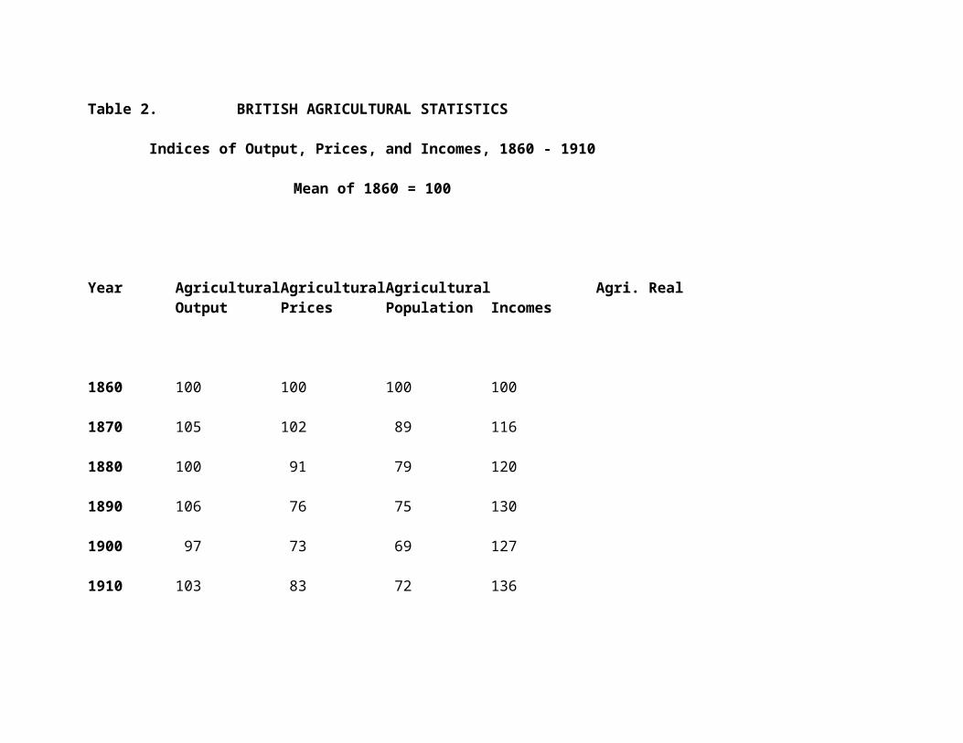
Table 11.

Shares of the Population of Great Britain Dependent on Imported Foreign Wheat

in percentages of total population and estimated number of consumersin decennial means, 1801-10 to 1901-14

Decade Percentage of Total Population

Estimated Number of Consumers of Foreign Wheatin millions

1801-10 7.0 0.8

1811-20 5.5 0.7

1821-30 4.9 0.7

1831-40 8.2 1.4

1841-50 18.4 3.6

1851-60 28.8 6.3

1861-70 42.8 10.5

1871-80 60.0 16.6

1881-90 70.0 21.9

1891-00 76.5 26.7

1901-14 83.4 32.9

Source:

Mette Enrnæs, Karl Gunnar Persson, and Søren Rich, ‘Feeding the British: Convergence and Market Efficiency in the Nineteenth-Century Grain Trade’, The Economic History Review, 2nd ser., 61: No. S1 (August 2008): Special Issue: Feeding the Masses, ed. Steve Hindle and Jane Humphries, pp. 140-71.

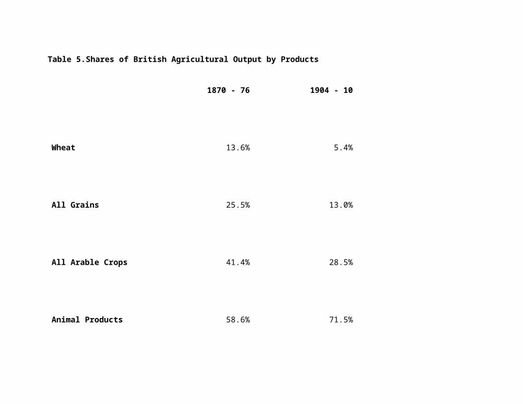
Table 12. The Populations of Selected European Countries in Millions, in decennial

intervals, 1800-1910

GreatYear Britain Belgium France Germany Russia

1800 10.7 3.1 27.3 n.a. 35.5

1810 12.0 n.a. n.a. n.a. n.a.

1820 14.1 n.a. 30.5 25.0 48.6

1830 16.3 4.1 32.6 28.2 56.1

1840 18.5 4.1 34.2 31.4 62.4

1850 20.8 4.3 35.8 34.0 68.5

1860 23.2 4.5 37.4 36.2 74.1

1870 26.0 4.8 36.1a 40.8b 84.5

1880 29.7 5.3 37.7 45.2 97.7

1890 33.0 6.1 38.3 49.4 117.8

1900 37.0 6.6 39.0 56.4 132.9

1910 40.9 7.4 39.6 64.9 160.7

a Excluding Alsace-Lorraine.

b Including Alsace-Lorraine.

Sources: B.R. Mitchell and P. Deane, Abstract of British Historical Statistics (Cambridge, 1962), pp. 8-10; Carlo Cipolla, ed., Fontana Economic History of Europe, Vol. IV:2 (1972), pp. 747-48.

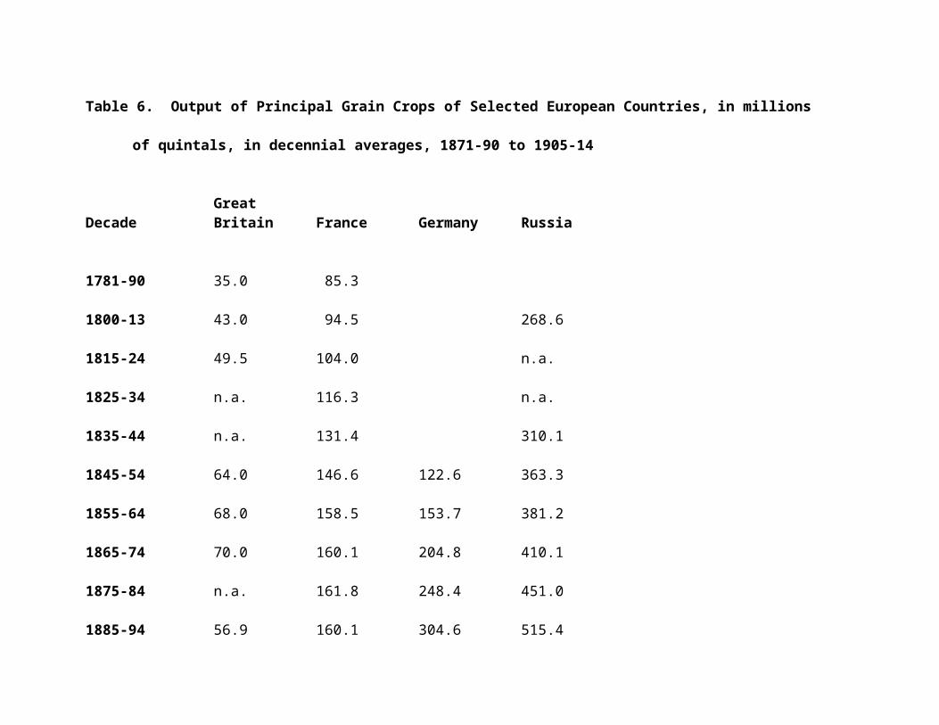
Table 13.Williamson: Real Wages in the US and Europe, 1861 - 1913

100 = Real Wages in Great Britain in 1905

Years Gr Britain U.S. Belgium France Germany

1861-65 61.20 87.60 50.80 45.00 56.20

1866-70 63.20 100.40 56.60 48.20 55.40

1871-75 74.00 120.60 66.00 50.60 61.60

1876-80 83.60 115.60 64.60 54.80 63.80

1881-85 88.00 129.60 71.00 59.60 66.60

1886-90 95.40 139.80 79.80 62.60 73.20

1891-95 100.00 145.00 83.00 63.60 75.60

1896-00 104.80 152.00 89.40 67.60 82.20

1901-05 100.40 163.00 85.80 71.60 83.40

1906-10 107.40 170.20 86.00 74.80 87.00

1911-13 105.00 166.67 88.67 65.33 89.00

Source: Jeffrey Williamson, ‘The Evolution of Global Labor Markets Since 1830: Background Evidence and Hypotheses’, Explorations in Economic History, 32 (1995), 141-96.

Table 14. Indices of Relative GDP per capita, compared to US GDP per capita (1.000)

for each year of the series

Country 1820 1830 1840 1850 1860 1870 1880 1890 1900 1913 1929 1938

United Kingdom

0.965 1.004 0.975 1.000 0.971 1.004 0.903 0.915 0.917 0.847 0.774 0.898

France 0.713 0.784 0.790 0.781 0.821 0.809 0.753 0.784 0.768 0.770 0.605 0.623

Nether-lands

0.800 0.768 0.814 0.791 0.766 0.787 0.708 0.735 0.715 0.668 0.594 0.704

Belgium 0.749 0.742 0.792 0.836 0.793 0.791 0.772 0.743 0.560 0.698

Germany 0.609 0.681 0.679 0.620 0.738 0.753 0.742 0.607 0.811

Austria 0.551 0.554 0.541 0.518 0.575 0.523 0.543 0.531 0.532 0.504 0.570

Denmark 0.513 0.584 0.616 0.661 0.626 0.659 0.618 0.644 0.668 0.667 0.662 0.741

Switzerland 0.687 0.726 0.741 0.726 0.674 0.761

Italy 0.641 0.589 0.535 0.525 0.512 0.526 0.472 0.529

Spain 0.638 0.638 0.554 0.564 0.567 0.521 0.511 0.463 0.331

Russia 0.410 0.445 0.452 0.451

Australia 1.022 1.174 1.370 1.096 1.304 1.130 1.049 1.085 0.976 0.976 0.860 0.924

Canada 0.827 0.834 0.828 0.740 0.809 0.853 0.968 0.900 0.914

Japan 0.265 0.307 0.335 0.375 0.412 0.440

Argentina 0.734 0.782 0.762 0.813 0.648 0.558

Source: Leandro Prados de la Escosura, ‘International Comparisons of Real Product, 1820 - 1990: An Alternative Data Set’, Explorations in Economic History, 37:1 (January 2000), 1-41.

Table 15:

CANADA: CONSUMER PRICE INDEX AND RELATIVE IMPORTANCE OF THE MAJOR COMPONENTS

February 2009Index: 2002 =

100

June 2007 June 2008 June 2007 Feb 2009 June 2008Percentage to June 2008 to Feb 2009

share of the per cent change

per cent change

components

All-items 100.00 111.90 115.40 3.13% 113.80 -1.39%

Food 17.04 112.60 115.80 2.84% 121.20 4.66%

Alcoholic beverages and tobacco products 3.07 125.70 127.70 1.59% 129.20 1.17%

Shelter 26.62 116.80 122.30 4.71% 123.20 0.74%

Household operations and furnishings 11.10 103.00 104.30 1.26% 106.40 2.01%

Clothing and footwear 5.36 93.10 92.50 -0.64% 93.60 1.19%

Transportation 19.88 119.20 125.80 5.54% 110.20 -12.40%

Health and personal care 4.73 107.90 108.70 0.74% 110.40 1.56%

Recreation, education and reading 12.20 102.50 102.90 0.39% 101.10 -1.75%

CANADA: CONSUMER PRICE INDEX AND RELATIVE IMPORTANCE OF THE MAJOR COMPONENTS

February 2009Index: 2002 =

100

All-items (1992=100) 100.00 133.20 137.30 3.08% 135.40 -1.38%

Source: Statistics Canada: http://www.statcan.gc.ca/

Note: in the Consumer Price Indexes used for England and the Low Countries, in the later-medieval and early-modern eras, up to the 18th century, foodstuffs – grains, meat, fish, drink – constitute an 80% weighting of the total index, compared to just 20% in this Canadian CPI.

Keep in mind that alcoholic products were, before the late 19th century, more of a necessity than a luxury: to provide bacteria-free beverages, or those known to be safe, when water and milk were so dangerous – before Koch’s and Pasteur’s discovery of the bacterial transmission of diseases, most of which were water-borne.