Weather variability and food consumption: Evidence from Uganda.

A Research Paper presented by:

Sara Lazzaroni

(Italy)

in partial fulfillment of the requirements for obtaining the degree of

MASTERS OF ARTS IN DEVELOPMENT STUDIES

Specialization:

Economics of Development

(ECD)

Members of the Examining Committee:

Prof. Dr. Arjun Bedi

Prof. Dr. Peter Van Bergeijk

The Hague, The Netherlands December 2012

ii

iii

Contents

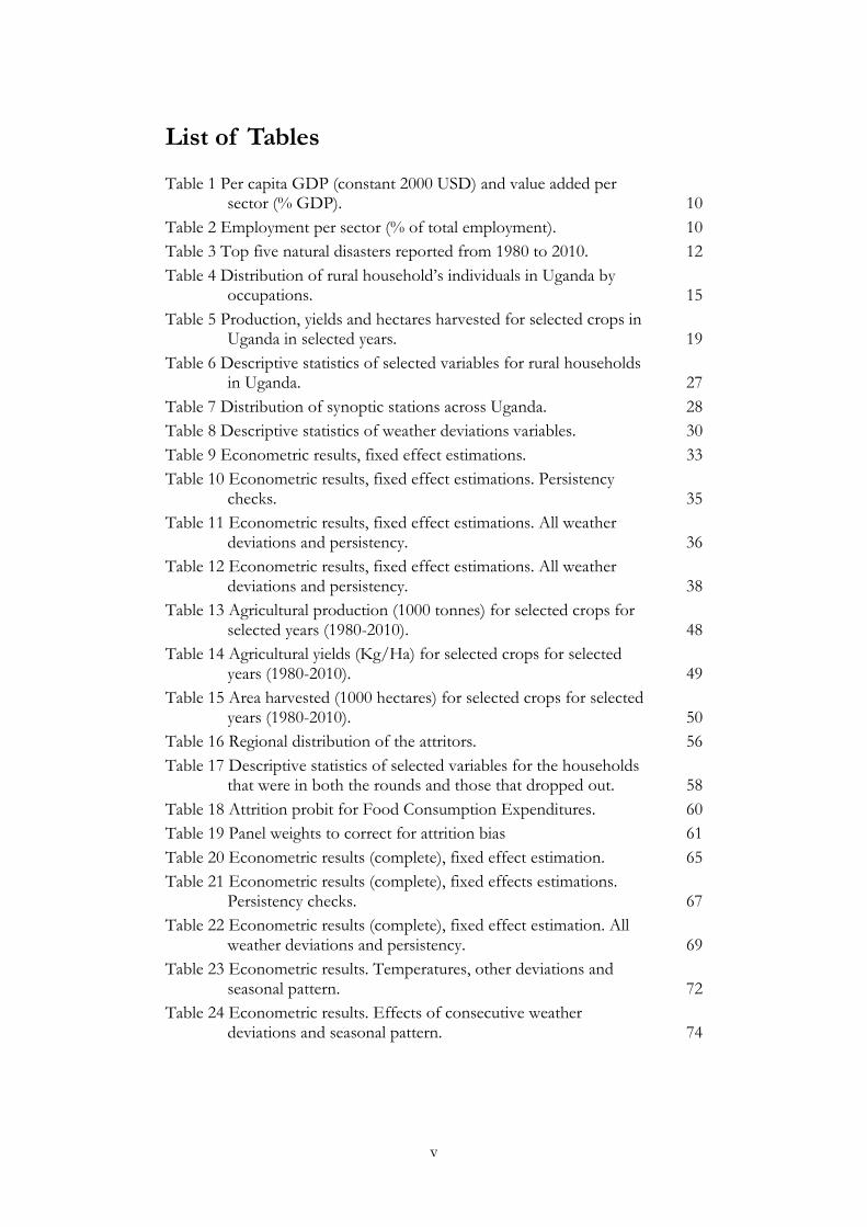
List of Tables v

List of Figures vi

List of Acronyms vii

Aknoledgments viii

Abstract ix

Chapter 1 Introduction 1

Chapter 2 Background and theoretical framework 4

2.1 Climatic shocks and welfare impacts 4

Climatic shocks 4

Welfare impacts 5

Coping mechanisms and adaptation 8

2.2 Weather variability and welfare in Uganda 10

Background 10

Uganda’s climate and recent changes 13

Agricultural productivity, income and consumption effects 15

2.3 Model Specification 19

Basic model 19

Choice of variables 21

Persistency 23

Heterogeneity of impacts 23

Chapter 3 The Data 25

3.1 Household data 25

3.2 Weather data 28

Chapter 4 Results 31

4.1 Average effects of weather deviations on food consumption 31

Rainfall, rainy days and temperatures deviations separately 32

Persistency 34

All weather deviation and persistency 35

Household socio-demographic variables 37

4.2 Heterogeneity of impacts 37

Chapter 5 Conclusions 40

iv

References 41

Appendices 48

Appendix A Agricultural production, yield and harvested area data for selected crops 48

Appendix B Distribution of monthly average long term mean for rainfall and temperatures for the 13 synoptic stations of Uganda 51

Appendix C Attrition detection and correction 56

Appendix D1 Results of specifications for 2005/06 cross-section. Dependent Variable: Log Food consumption 62

Appendix D2 Results of specifications for the 2009/10 cross-section. Dependent Variable: Log Food consumption 63

Appendix D3 Results of specifications for the pooled cross-sections. Dependent Variable: Log Food consumption 64

Appendix E Complete results of specifications (1)-(16). Dependent Variable: Log Food consumption 65

Appendix F Effects of weather deviations in particular seasons 71

Appendix G Effects of persistency in weather deviation and seasonal pattern 73

Appendix H Map of Uganda with synoptic stations 75

v

List of Tables

Table 1 Per capita GDP (constant 2000 USD) and value added per sector (% GDP). 10

Table 2 Employment per sector (% of total employment). 10

Table 3 Top five natural disasters reported from 1980 to 2010. 12

Table 4 Distribution of rural household’s individuals in Uganda by occupations. 15

Table 5 Production, yields and hectares harvested for selected crops in Uganda in selected years. 19

Table 6 Descriptive statistics of selected variables for rural households in Uganda. 27

Table 7 Distribution of synoptic stations across Uganda. 28

Table 8 Descriptive statistics of weather deviations variables. 30

Table 9 Econometric results, fixed effect estimations. 33

Table 10 Econometric results, fixed effect estimations. Persistency checks. 35

Table 11 Econometric results, fixed effect estimations. All weather deviations and persistency. 36

Table 12 Econometric results, fixed effect estimations. All weather deviations and persistency. 38

Table 13 Agricultural production (1000 tonnes) for selected crops for selected years (1980-2010). 48

Table 14 Agricultural yields (Kg/Ha) for selected crops for selected years (1980-2010). 49

Table 15 Area harvested (1000 hectares) for selected crops for selected years (1980-2010). 50

Table 16 Regional distribution of the attritors. 56

Table 17 Descriptive statistics of selected variables for the households that were in both the rounds and those that dropped out. 58

Table 18 Attrition probit for Food Consumption Expenditures. 60

Table 19 Panel weights to correct for attrition bias 61

Table 20 Econometric results (complete), fixed effect estimation. 65

Table 21 Econometric results (complete), fixed effects estimations. Persistency checks. 67

Table 22 Econometric results (complete), fixed effect estimation. All weather deviations and persistency. 69

Table 23 Econometric results. Temperatures, other deviations and seasonal pattern. 72

Table 24 Econometric results. Effects of consecutive weather deviations and seasonal pattern. 74

vi

List of Figures

Figure 1 Weather variability and its impact on household welfare. 6

Figure 2 Agricultural cycle in Uganda. 29

Figure 3 Example of the mechanism of assignment of weather deviations. 29

List of Maps

Map 1 Map of Uganda (regions and districts) with the 13 synoptic stations. 74

vii

List of Acronyms

BOU Bank of Uganda

CRED Center for Research on the Epidemiology of Disasters

DRC Democratic Republic of Congo

EAs Enumeration Areas

EM-DAT Emergency Event Database

FAO Food and Agriculture Organization

GoU Government of Uganda

ISDR International Strategy for Disaster Reduction

IPCC Intergovernmental Panel on Climate Change

ISS Institute of Social Studies

LRA Lord’s Revolutionary Army

LSMS Living Standard Measurement Study (World Bank)

MAAIF Ministry of Agriculture

NAPA National Adaptation Programmes of Action

UBOS Uganda Bureau Of Statistics

UDOM Uganda Department of Meteorology

UNHS Uganda National Household Survey

UNDP United Nations Development Programme

UNPS Uganda National Panel Survey

WB World Bank

viii

Acknowledgments

This has been an intense year, full of people, cultures, experiences, places and, overall, knowledge and emotions. Trying to list the people that I have to thank mentioning their role in this 15 months would require another RP to be writ-ten.

In any case, first of all I have to thank my Family for the constant support from home, without you and your love, I wouldn’t be the person that I am to-day.

Second, I have to thank my supervisors for the guidance and support dur-ing the year and in the writing of this thesis. Enthusiasm sometimes faded away but they were able to always motivate me to do my best, handling the ups and downs that life brings with its constant flowing.

Last, but not least, I have to thank the people that I have met here and that have accompanied me throughout this experience. My thanks go especially to those wonderful ones that have been close enough to me to go beyond the surface and get to know me in my (good and bad) entirety. You will never lose the special place that I gave to you in my heart.

Praise to God that gave me all this.

ix

Abstract

In the wake of the continuing debate on the effects of climate change on households’ wellbeing, this study considers the impact of short-term weather variations, as an indicator of climatic change, on food consumption of rural households in Uganda. After defining and placing climatic shocks in the litera-ture on shocks and vulnerability, the paper explores the channels through which weather variations may affect rural household welfare in the context of a subsistence agricultural system such as Uganda. For the purpose of the analy-sis, we combined households data from the World Bank LSMS panel dataset on Uganda covering the period 2005/06-2009/10 with weather data from 13 synoptic stations across the four regions of the country. Weather variations were described by rainfall, number of rainy days and temperature deviations from their respective long term means calculated over the period 1960-90 (1980-2010 for temperatures) thanks to data compiled by the Ministry of Water and Environment, Department of Meteorology of Uganda. The results of the empirical model suggest that weather variability has relatively minor effects on food consumption. In particular, household welfare is affected by deviations in the number of rainy days and minimum temperatures with the effects depend-ing on the season in which they occurred.

The relatively minor impact of weather variations on food consumption, combined with the analysis of other studies and agricultural sector recent de-velopments showing relatively small effects of climatic shocks, suggests that rural households are involved in ex-ante income smoothing strategies that in-sure them from the adverse effects of weather variability on food consumption in the country. Future research should examine the effects of weather variabil-ity on agricultural production or income generation process in order to obtain a better understanding of how households may have been adapting to weather changes.

Relevance to Development Studies

In light of the concerns about climate change effects on households’ welfare, this study attempts to analyze the impact of short term weather variations as indicators of a change in the pattern of climate. However, as the study has sug-gested, poor rural households have been able, to a certain extent, to adapt to continuous changes in weather indicators in such a way that their food con-sumption is only slightly affected by shocks to the agricultural production and income, although agriculture is still conducted on a subsistence basis. In light of this, catastrophic predictions on the potential effects of climate change, at least in the current context, seem to be exaggerated. Attention should be given to understand how to enhance households adaptation strategies to fully ensure their welfare from adverse climatic shocks. In particular, Uganda appears to be an example of ex-ante adaptation to the (not much explored) potential effects of climatic shocks in the country.

Keywords

Weather variability, food consumption, Uganda.

1

Chapter 1 Introduction

Climate change has been defined by the Intergovernmental Panel on Climate Change as “any change in climate over time, whether due to natural variability or as a result of human activity”(IPCC 2001: 22). Lots of words have been spent on this phenomenon since the ‘90s and the research and the discourses around it are now common in the academic and daily life. With this respect, we have that the debate around climate change has moved from the discussion about the reality, sources and possible effects of it to the treatment of it as a fact, even though there is still lot of uncertainty about the actuality and magni-tude of its consequences (Crist 2007: 29). Besides, when considering the im-pact of atmospheric phenomena on indicators of interest, a crucial distinction has to be put forward between weather and climate. In fact, while the former can be defined by the atmospheric hourly and daily fluctuations as captured by temperature, humidity and precipitation data, climate is defined as “the prevail-ing weather, describing both the average conditions and the variations (and distributions) [in a time-series perspective] of weather conditions for some par-ticular geographical locality or region” (Stenseth et al. 2003: 2088). Hence, weather variability can be considered ultimately a signal of climate change to the extent that it departs from the average prevalent atmospheric condition measured in the past and it is a source of change in the long-term pattern of climate for the location considered. This being said, as entrepreneurs and pro-ponents of agricultural development have agreed, it is in the context of devel-oping countries, and especially in Sub Saharan Africa, that changes in the weather patterns bite more because of the high degree of vulnerability1 that individuals and households in these countries experience (Cooper et al. 2008: 25). In addition, when it comes to analysing climate variations in developing countries, the intellectual challenge is very high due to constraints on the avail-ability of historical data and the complexity of the context at hand in terms of modeling, national and international stakeholders involved and available policy options (ibid: 12). Finally, as mentioned before, since climate change is a phe-nomenon that requires long time to materialize because it generally takes place trough small changes in the pattern of weather cycles and weather indicators, in the process of development the constant improvements in technology have been able, to a certain degree, to mitigate the impacts of weather changes on individuals and economic activities (Nordhaus 1993: 14). To the extent than developing countries have been able to appropriate or develop these technolo-

1 For a comprehensive definition of vulnerability in the context of climate change re-search refer to Füssel (2007). In a broader sense here we consider the cross-scale inte-grated vulnerability, namely, the one that is a combination of internal and external scale and socio-economic and biophysical domains. On the other side, in applying our empirical analysis we will make use of Dercon’s concept of risk-related vulnerability, that is “the exposure to risk and uncertainty, the responses to these, the welfare con-sequences, and the implications for policy” (Dercon 2006: 2).

2

gies, then, they have been able to cope or, as the literature on climate change states, adapt2, to climatic shocks3.

Traditionally, the relationship between weather vagaries (and more gener-ally natural hazards or shocks) and people’s welfare in developing countries has been analysed in the context of the dependence of these countries on the rain-fed agricultural sector as the main source of income. It’s mainly due to this rea-sons that climate change constitutes a threat to the development of these economies (Skoufias et al. 2011: 2). However, households in rural areas are not the only one affected: the increase in urbanization in developing countries also poses challenges to the wellbeing of urban households, overall as far as the management of water resources and health is concerned. In fact, in a limited space cities can concentrate a high number of individuals, households, activi-ties, sectors and infrastructures. The impact of shocks could then be exacer-bated in urban contexts that are under the pressure of many socio-economic actors and factors within the same limited area (Hallegatte et al. 2011). At the same time, analysing both the rural and urban households in the same frame-work doesn’t constitute the optimal strategy since the context of rural areas is completely different for the opportunities, challenges and mechanisms in which people are involved. For example, an extensive period of drought is likely to impact primarily on rural households due to their dependence on the agricultural or natural resources-dependent sectors, while the impact on urban households is more through the availability of drinkable water and food prices, not much directly on the economic activities in the city (Satterthwaite et al. 2007: 27). Moreover, rural and urban households differ for their income pat-tern and diversification, and the impact and coping methods in reaction to cli-matic shocks. For instance, in his work on Zimbabwe Ersado (Ersado 2005) found out that in the early ‘90s wealthier urban households had less diversified income sources while the contrary was happening for rural households. How-ever, after two severe droughts and the implementation of the Economic Structural Adjustment Program (climatic and economic shocks combined) the wealthier rich had diversified income sources like the rural counterparts in or-der to better cope with the shocks.

With these premises in mind, this paper attempts to analyse the impact of weather variability in the period 2005/06-2009/10, measured as the deviation of rainfall, number of rainy days and temperatures from their long term mean, on the wellbeing of rural households in Uganda. In connection with our previ-

2 Although the terms cope and adapt are often used interchangeably (see Smit and Wandel (2006) for a review of the conceptualization of adaptation to realize how the two terms have been linked in the literature), we agree with the differentiation made by Peltonen (2005). The author distinguishes between short term coping capacity that individuals use to immediately respond to a shock, and long-term adaptive capacity that entails learning processes on how to deal with the phenomena at hand (ibid). 3 Here we have to make a specification that will be clearer also in the following sec-tion: with the term “climatic shocks” we mean variations from the general pattern of rainfall (including droughts and floods), temperatures as well as crop pests and dis-eases caused by weather deviations in a specific period of time. In other words, in this case the attribute “climatic” does not explicitly refer to the long-term phenomena of climate change but to short-term weather deviations (from the general pattern of cli-mate).

3

ous discussion, since weather variations can be considered markers of climate change, we are going to calculate our weather variables as deviations from the 1960-1990 and 1980-2010 long term means4 in order to not incorporate in the long term means the effects of more recent climate change (similarly to the approach of Skoufias et al. (2011)). Indeed, despite the increasing importance of climate change in the country (highlighted for example by Magrath (2008)), and the availability of weather data dating back to the 1960s, we only have a households microeconomic dataset covering the period aforementioned. Hence, the choice to concentrate on the impact of more short-term weather variations. Moreover, we will concentrate on those households that were living in rural areas in both the rounds of the panel dataset, since we want to specifi-cally take care of the rural dimension of the impact of climatic shocks.

In order to quantify the impact of weather variability on the welfare of households in Uganda we will make use of the 2005/06-2009/10 Living Stan-dard Measurement Study (LSMS) panel dataset provided by the World Bank on Uganda and we will concentrate on the food consumption variations in the country, this choice motivated also by the concerns about food security in the country (Shively and Hao 2012). For the purpose of the analysis, the LSMS data will be merged with rainfalls and temperatures recordings made by the Ministry of Water and Environment, Department of Meteorology of Uganda.

To begin with, we will situate climatic shocks in the literature on shocks in developing countries and we will analyse the channels through which they af-fect households welfare. Moreover, we will briefly introduce the possible cop-ing and adapting strategies available to households to mitigate the impact of these shocks. After, we will contextualize the previous analysis in the case of Uganda, highlighting the main aspects that weather variability affects. In order to go from the general to the specific approach we will start from recent re-ports on the state of the country and move towards a review of recent applied works dealing also with the coping and adaptation strategies in which rural households have engaged in response to climatic shocks. Finally, after a de-scription of the weather and socio-economic characteristics of the country, with a special attention to the agricultural sector due to its close connection with rural households wellbeing, we will proceed with the empirical analysis of the impact of weather variability in Uganda.

The remainder of this paper is organized as follows. Section 2 presents climatic shocks and the channels through which they affects households wel-fare firstly with a general approach and then specifically in the case of Uganda. Section 3 deals with the empirical analysis while Section 4 reports the results. Section 5 concludes.

4 We will use the 1960-1990 long term means for rainfall millimetres and number of rainy days and the 1980-2010 long term means for maximum and minimum tempera-tures. The change in the period of reference for the long-term means calculation is due to data constraints.

4

Chapter 2 Background and theoretical framework

2.1 Climatic shocks and welfare impacts

Climatic shocks

Within the field of development economics and particularly in connection with the study of the determinants of poverty, much of the emphasis has been put on the role of risk, shocks and vulnerability. Furthermore, in the last decade the analysis of the context of developing countries has been more and more relying on micoreconometric techniques to understand which type of shocks5 and how they impact on individuals and households welfare. In particular, it is in the African setting that the analysis of the impact of shocks and coping strategies on households welfare now constitute a quite large body of literature.

In their work on Ethiopia, Dercon et al. generally defined shocks as “ad-verse events that lead to a loss of household income, a reduction in consump-tion and/or a loss of productive assets” (Dercon et al. 2005: 5). The authors classified shocks into five broad categories. First of all, there are the climatic shocks, namely, those disturbances in the usual pattern of rainfall and tempera-tures but also complex events like droughts and floods and other climate-induced distresses affecting crops and livestock such as pests and diseases. Second, economic shocks affecting access or prices of inputs and outputs on the market. Third, political, social and legal shock (for example conflicts, dis-criminations or disputes), that we put together with crime shocks (theft and crimes towards the individuals). Finally health shocks such as illnesses and death. As expressed in our introduction, we will concentrate on the first cate-gory, climatic shocks, because, as Tol has stated in his review of the economic effects of climatic variability, these shocks can be considered “the mother of all externalities” (Tol 2009: 29). Indeed, amongst the different measurable dimen-sions of welfare6, unexpected weather changes can potentially affect all of them because unexpected weather changes, especially if they come with high magni-tude (in the form of a severe drought or flood), constitute a pervasive phe-nomenon affecting “agriculture, energy use, health and many aspects of na-ture” (ibid)7. Moreover, their effects are long-lasting. For example, in a paper

5 For example, a macro classification is the one between covariate or idiosyncratic shocks, the former happening at a aggregate level and the latter at the individ-ual/household level. 6 Espig-Andersen (2000: 8) lists welfare components according to a resource-view of welfare. Her classification comprises income and monetary-equivalent resources; health; housing; family, social integration and networks; free time and leisure; working life; political resources; insecurity. 7 If we consider weather variability as a result of climate change, this phenomena is pervasive also on the side of the producers because almost every activity and person produce greenhouse gases, and even more worrisome, their long-lasting effects are likely to affect more those that contribute less to the propagation of the phenomena, namely, people in low-income countries (Tol 2009: 29).

5

analysing 342 rural households in Ethiopia in the period 1989-1997 Dercon (2004) found that 1% lower current food consumption growth rates were ex-plained by a 10% decrease in rainfall that had taken place 4-5 years earlier. Analogously, Newhouse (2005) revealed that 30% of the 1993 rainfall shock on the income of Indonesian rural farm households persisted in determining farm income in 1997. On the other side and looking to other welfare indicators in the context of Indonesia, Maccini and Young (2008) found a positive impact on women that experienced 20% more rains at the year of birth on self-reported health, height, education attainments and household asset index when they were adults. Hence, the importance of analysing the impact of climatic shocks on households welfare.

Welfare impacts

In discussing the effects of climatic shocks on households welfare, we may re-fer to the 2001 report of the Working Group II to the Third Assessment Re-port of the IPCC (IPCC 2001) and support its claims with the findings in the microeconomic literature. The IPCC has classified the projected changes in climate into two broad categories: simple extremes and complex extremes (ibid: 29). Within the former we can find higher maximum and minimum tem-peratures (with the connected increase of hot days and heat waves) and the increase in the intensity of precipitation events. An increasing occurrence of droughts and floods, especially when precipitations are associated with El Niño events, of storms and tropical cyclones and more variability in the monsoon season are, instead, some examples of extreme events (ibid). Coming to the impact of the two kinds of events on welfare8, we follow the approach of Skoufias et al. (2011) and discuss some aspects of rural households welfare. In doing this, we refer to Figure 1 to visualize the chain of effects that climatic changes causes. The solid lines represent direct effects while the dashed lines represent indirect effects. Then, for our analysis we will concentrate on one of the aspects discussed: food consumption.

First of all, weather variability impacts on economic activity in different sectors, nevertheless, the agricultural one is likely to be the most affected for its close connection with the natural system. This, combined with the importance of agriculture in developing countries, implies that weather variability can have an impact on the performance of the entire economy. According to the IPCC (2001: 31), weather variations have a direct impact on the agricultural produc-tivity and consequently on the agricultural income since higher temperatures and changing rainfall patterns are likely to change the hydrological cycle9, ulti-

8 In this work we don’t separate the analysis of the two kinds of extreme events be-cause, as suggested by Anderson (1994: 555), complex events are nothing but simple extreme events that occur in a more disruptive way due to their particular duration and temporal shape. 9The hydrological cycle is the process through which water circulates among the oceans, atmosphere and biosphere by evaporation, condensation and precipitation (Chahine 1992). According to the FAO (1995), among the major weather variables, temperatures, evaporation and rainfall are those that are more likely to accelerate the water cycle, ultimately changing the spatial and temporal (daily/seasonal) distribution of water in the different ecosystems (the other variables considered were cloudiness, wind and evapotranspiration potential).

6

mately affecting crop yields and total factor productivity. In fact, according to Lansigan et al. (2000) weather changes have short-term impacts on crop yields through changes in temperatures when they exceed the optimal thresholds at which crops develop10. Moreover, mismatches between the amount of water received (and its potential evapotranspiration) and required along the growing and harvesting seasons, and the timing of the water stresses faced by the crops, also affect the agricultural productivity11. For example, Skoufias et al. (2011) showed negative consumption responses to colder weather shocks during the pre-canícula season in the Northern region of Mexico. On the other side, when water comes or doesn’t come in extreme quantities, its potential impact can be very high due to the potential losses of lives and infrastructures for example in the case of floods (IPCC 2001: 29). Note here that, as Arnell has argued, water resources infrastructure characteristics are crucial in determining the impact of weather variability on human and natural systems wellbeing (Arnell 1998: 84). Hence, the need of a constant rethinking of the structures implemented for water management, especially in developing countries where water scarcity is combined with problems of water quality and accessibility.

Figure 1 Weather variability and its impact on household welfare.

Source: Adapted from Skoufias et al. (2011).

Going back to our chain of effects, an instability or a decrease in agricul-tural income will have effects on consumption (a share of income), depending on the subsistence nature of the agricultural activity or on the price of the pur-

10 For instance, Prasad et al. (2008) demonstrated that sorghum exposed to high tem-perature stress was subject to a delay in the inflorescence and lower height, number of seeds and yields. 11 For example, Wopereis et al. (1996) found that a reduction in water at the vegetative stage of rice can reduce its morphological and physiological characteristics while droughts at the stage of reproduction can sensibly lower the yields. Similarly, Otegui et al. (1995) revealed that maize that suffered prolonged shortage of water at silking was subject to yield reduction.

7

chased products. Indeed, when the agricultural activity is of subsistence, the effect on consumption is through the quantities produced while in the case of market-oriented activity, the effect can be both through quantities and prices. In the latter case, according to the Agricultural Household Model there could be a positive net effect on households income and then consumption (Singh et al. 1986) but this doesn’t seem to be the case in the context we will analyse due to the prevalence of subsistence agriculture in the country12. The impact of de-creased income will affect different types of consumption in different ways. Generally, food consumption is likely to decrease less that non-food consump-tion (Skoufias and Quisumbing 2005) but this behaviour can depend on household characteristics (for example on the sex of the income earner as in Duflo and Udry (2004)). Moreover, even when the yield is more or less the same, erratic weather can stress the crops and lower the quality of the harvest.

The indirect impacts of weather changes come firstly from their direct im-pact on the individual health and secondly as the outcomes of a reduction of income and consumption at the household level. The first is explained by the fact that weather variability affects the productivity in the agricultural sector. These effects are symbolized in Figure 1 by the dashed arrow (indirect effect) pointing from the development of vector/water/food-borne diseases to the agricultural productivity, the former being a direct consequence of weather variations on parasites life cycles. In fact, weather provide those conditions that allow pathogens already existing in the environment to develop and spread or make their life longer than their usual historic range (Anderson et al. 2004: 540). This applies for infectious diseases of plants and animals13 and to human being as well. For example, Piao et al. (2010) have shown in a recent study on China that changed local ecology of water borne and food borne infective dis-eases can cause an increase in the incidence of infectious diseases and crop pests. Similarly but concerning human beings, the research has highlighted that individuals are affected in different ways14 by changes in illness and death rates as well as injuries and psychological disorders due to higher temperatures or complex extreme events such as floods and storms. For instance, some authors cite as examples of vector-borne diseases sensitive to climatic changes the mosquitoes responsible of malaria, filariasis, dengue fever, yellow fever; sand-flies causing leishmaniasis and tsetse flies bringing African trypanosomiasis (Haines et al. 2006: 2104). In addition, also infectious diseases and diarrhoea are likely to increase due to the prolonged range and activity of pathogens (ibid). This being said, the productivity of the labour force, especially in the agricultural sector, is potentially highly affected.

12 This argument is further supported by Benson et al. (Benson et al. 2008). The au-thors analysed the mechanism of global and regional prices transmission and its wel-fare effects in Uganda suggesting that not many would benefit from rising food prices. In fact, only 12 to 27% of the population seems to be a net seller of food. 13 For example see the study by Anderson et al. on the impact of climate change on plants diseases: “Climate change can lead to disease emergence through gradual changes in climate (e.g. through altering the distribution of invertebrate vectors or increasing water or temperature stresses on plants) and a greater frequency of unusual weather events (e.g. dry weather tends to favour insect vectors and viruses, whereas wet weather favours fungal and bacterial pathogens)” (Anderson et al. 2004: 540) 14 McMichael and Haines (1997) highlighted that health effects are different for indi-viduals depending on their sex, age, living and poverty conditions.

8

Finally, the malnutrition effects on human capital are one of the most ex-plored phenomena following lower food productivity through the food con-sumption effects of weather vagaries (de la Fuente and Dercon 2008). Malnu-trition affects adults and children in different ways15. If adult malnutrition is an important problem because it has an impact on productivity on the workplace, children malnutrition can have very detrimental effects also in the long run16. Household members state of health can differ due to the choices in the alloca-tion of the food to the different components (Skoufias et al. 2011: 6). Then, in connection with problems of food security and malnutrition, lower BMI and labour productivity for the adults as in the study by Dercon and Krishnan in Ethiopia (Dercon and Krishnan 2000: 6), and children stunted growth, as demonstrated by Yamano et al. (Yamano et al. 2005), are examples of the indi-rect impacts of a reduction of household income and consumption on individ-ual health. Concluding our analysis of the channels through which weather variations can affect human wellbeing, we have to highlight the fact that weather changes will affect households and individuals depending on the ex-ante and ex-post coping mechanism that they are able to put in place.

Coping mechanisms and adaptation

According to Morduch (1995: 104) there are two possible strategies that households can adopt in order to cope with risk: income smoothing and con-sumption smoothing.

Income smoothing consists of those decisions concerning production, employment and the diversification of the economic activities. On the produc-tion side, rural households can chose different types of crops to be cultivated and input intensities (ibid: 104). However, despite ensuring a certain amount of income, these strategies can have also adverse effect on households final wel-fare. For example, Dercon (1996) analyzed the interdependence of the crop choices between low-risk, low-return crops (sweet potatoes in the paper) and household’s consumption security derived by the ownership of liquid assets in Shinyaga District of Tanzania. The author found that, in the absence of devel-oped markets for credit, combined with the lack of accessibility to off-farm labour, households were cultivating sweet potatoes, hence obtaining less in-come and less possibility to build assets for the future. A poverty trap of low-income and assets ownership, induced low-risk, low-return crop choice (to fur-ther ensure against possible income and consumption losses due to the cultiva-tion of higher-return, higher-risk crops) and hence low-income and assets ac-cumulation seemed to capture households in the district studied (ibid). Another possible income smoothing strategies in the rural activity is the use of

15 For instance, a study on Ethiopia by Dercon and Krishnan found that adult BMI decreased by about 0.9% in those areas characterized by fewer rains and less strong consumption smoothing strategies (Dercon and Krishnan 2000). 16 A study on Zimbabwe, Alderman et al. (2006).found that adolescents that experi-enced drought when they were between 1 and 2 years old were 2.3 centimetres shorter, enrolled 3.7 months later and had 0.4 grades of retard in school grade com-pletion. Similarly, Maccini and Yang (2008) showed that early-life rainfall increased the height and school grade completion and decreased (self-reported) morbidity of Indo-nesian women borne in the period 1953-1974 most probably reflecting higher agricul-tural output in those years.

9

intercropping (that combines mixed cropping with field fragmentation) or adoption of new production technologies (like high-yielding varieties-HYV and fertilizers) to lower the risk of the agricultural activity. In this case, authors have demonstrated that behavioural norms and households specific character-istics play a further important role in the decision process (for example Foster and Rosenzweig (1995) showed that rural households in India adopted the HYV depending on the level of own and neighbors’ experience and initial asset stocks).

On the other side, consumption smoothing comprises decisions regarding borrowing and saving, selling or buying non financial assets (Fafchamps et al. 1998)(Fafchamps et al. 1998), modifying the labour supply and making use of formal/informal insurance mechanisms (Bardhan and Udry 1999: 95). For ex-ample, Paxon (1992) found that household in Thailand were able to use sav-ings to compensate for losses of income due to rainfall shocks, hence leaving consumption unaffected. The case of informal insurance schemes at the village level was instead revealed by Dercon (2004) in his analysis of food consump-tion growth in 342 rural communities in Ethiopia. The author showed that the households considered were able offset the risk of consumption losses from shocks at the household level (idiosyncratic shocks) thanks to the allocation of the risk within the village. This was supported by the fact that in the same con-text households were not able to ensure against rainfall shocks that were affect-ing all the households in the village (aggregate or covariate shocks)17. We will discuss the decisions about labour supply later on in the discussion of the case of Uganda where they have been tested by Kijima et al. (2006).

Thus we can say that income and consumption smoothing differ in the time horizon over which they deal with shocks: income smoothing is aimed to prevent or mitigate the effects of shocks before they occur while consumption smoothing is concerned with the effects of shocks after they have taken place. Then, when we try to estimate the effects of shocks occurred in the past on the actual measured outcome variable, it may be that we cannot find any effect precisely because households have engaged into one (or more) of these mechanism. The possibility to involve in coping mechanisms in response to short term weather variations and towards longer-term adaptation strategies to persistent climatic shocks is then crucial in mitigating the final impact of ad-verse events on households welfare. In the discussion of the impact of weather variability in Uganda, hence, we have to take into account the issues just raised. First of all, given the general vulnerability of the agricultural sector to weather changes due to the lack of irrigation systems and the use of traditional prac-tices, the recent less stable weather (possibly due to the process of climate change) could have pushed households to put in palce ex-ante/ex-post measures. In the next section we will then explore the performance of the agricultural sector since most of the households are employed in it and, overall, a big framework of modernization of this sector (the Plan for Modernization of Ag-riculture – PMA) the has been guiding since 2000 investments and interven-tions in “agricultural research, advisory services, rural finance, agro-processing and marketing, rural infrastructure, agricultural education and sustainable natu-

17 The lagged village average consumption was able to explain part of the household food consumption growth while the coefficients on the idiosyncratic shocks were not significant.

10

ral resource management” (MAAIF 2010: 27). Second, weather variations can be considered a country-level exogenous shock to the households in Uganda, if the chain of weather effects on agricultural productivity and income is not “compromised” by coping strategies, the coefficients on the weather deviations variables that we will use should significantly affect food consumption. Never-theless, the weather deviations recorded have a certain variability on regional and synoptic station area level. Hence, it may be that the food consumption of the areas adversely affected is compensated by the production obtained in other areas of the country. Notwithstanding this remark, the fact that the agri-cultural activity is mainly for subsistence constitutes a deterrent from consider-ing weather variations a sort of idiosyncratic shock in a country-level analysis.

2.2 Weather variability and welfare in Uganda

Background

Uganda is a landlocked country classified by the World Bank as a low income nation. Poverty in Uganda is high, nevertheless, there has been a decline in re-cent years. In fact, the percentage of population living with or less than 2$ a day (PPP) declined from 86% of the mid-nineties to about 76% in 2006, reach-ing 65% in 2009 (World Bank. 2011b). As Table 1 and 2 show, although the agricultural sector share of total GDP has decreased during the years, the country is still highly reliant on agriculture for the generation of its income, the agricultural sector employing more than 60% of the labour force (ibid).

Table 1 Per capita GDP (constant 2000 USD) and value added per sector (% GDP).

1990-1994 1995-1999 2000-2004 2005-2010

GDP per capita

(constant 2000 UDS) 193.99 239.11 273.38 345.13

Agriculture

value added (% GDP) 52.40 43.41 26.61 24.60

Industry

value added (% GDP) 12.72 17.17 23.22 25.75

Services

value added (% GDP) 34.88 39.42 50.17 49.65

Source: World Bank (2011b)

Table 2 Employment per sector (% of total employment).

2002 2005 2009

Agriculture 65.50 71.60 65.60

Industry 6.50 4.50 6.00

Services 22.00 23.20 28.40

Source: World Bank (2011b)

Note: Data on employment per sector are available only for the years presented in the table when a national household survey was conducted.

The fact that the economy and the livelihoods of many households and individuals is highly dependent on rain-fed agriculture makes the country par-ticularly vulnerable to weather changes and, more generally, to climatic shocks

11

(Mubiru et al. 2012: 1). Indeed, the unreliability and variability of onset, cessa-tion, amount and distribution of rainfall has led, according to Mubiru et al. to a decrease in agricultural productivity, especially for small farmers using back-ward techniques (ibid). However, convincing empirical studies quantifying the impact of weather variations on production, income and consumption in Uganda are missing18. Hence, the need to unveil if and how weather variations affect the rural households in the country to understand the risk that they face and if they are or not already able to ensure against it. In the former case, we will have some lessons learnt on the management of climatic shocks by rural households in Uganda while in the latter we will have to investigate adequate measures to counteract possible decreases in welfare.

Starting with a general view of the context at hand, rough estimates on the disaster profile of Uganda can be drawn from the Emergency Events Database (EM-DAT) maintained by the Center for Research on the Epidemiology of Disasters (CRED) at the Catholic University of Leuven, Belgium19. As we can see in Table 3, droughts and floods are those phenomena that mostly have af-fected the Ugandan population, even if they are not the main cause of deaths in the country. Nevertheless the registered events with the maximum amount of deaths is again hydrological (while the most killing events are epidemics20). The data on the economic losses are of course biased towards those disasters that involve a destruction of physical capital, the earthquake of 1994 dominat-ing this ranking. However, again droughts and floods appear as highly impor-tant in Uganda. Moreover, according to the 2009 Global Assessment Report, Uganda has more than 10% of its population exposed to the risk of droughts and it is listed as 19th out of 184 countries in the human exposure ranking for this type of hazard. Finally, Uganda has also a high to very high vulnerability index (in increasing order) for floods, earthquake and landslides (ISDR 2009).

18 The only empirical study we found on the impact of weather changes in Uganda is the one by Asiimwe and Mpuga (2007). We will discuss it later on. 19 EM-DAT contains essential core data on the occurrence and effects of over 18,000 mass disasters in the world from 1900 to present. It is compiled from various sources, including UN agencies, non-governmental organisations, insurance companies, re-search institutes and press agencies. This database contains information about disas-ters in the world that satisfy at least one of the following criteria: 10 or more people reported killed, 100 or more people reported affected, declaration of a state of emer-gency or call for international assistance. Earthquakes, floods, droughts, extreme tem-perature events and landslides are some of the phenomena recorded in the sample. 20 An epidemic is defined by EM-DAT as “either an unusual increase in the number of cases of an infectious disease, which already exists in the region or population con-cerned; or the appearance of an infection previously absent from a region” (EM-DAT. 2012).

12

Table 3 Top five natural disasters reported from 1980 to 2010.

Top 5 Disaster Date Affected

Affected people

(no. of people)

Drought 2008 1,100,000

Flood 2007 718,045

Drought 1999 700,000

Drought 2002 655,000

Drought 1987 600,000

Killed people

(no. of people)

Mass movement wet21 2010 388

Epidemic 2000 197

Epidemic 1990 156

Epidemic 1989 115

Drought 1999 100

Economic damages

(US$ x 1,00022)

Earthquake 1994 70,000

Drought 1998 1,600

Flood 1997 1,000

Flood 2007 71

Epidemic 1982 0

Source: Adapted from www.preventionweb.net, accessed 30 June 2012.

Again from a nation-wide perspective, the National Adaptation Plan of Action elaborated in 2007 summarizes the five channels through which climate change is impacting on Uganda’s development. Firstly the health sector has been affected in the latest decades since waterborne diseases such as malaria, diarrhoea and cholera and respiratory diseases spread in a easier manner as the occurrence of floods increased and/or long dry spells took place (NAPA 2007: 11). Moreover, climatic changes impinge on food production that in turn has an impact on health through malnutrition, lowering children wellbeing and adults productivity and, ultimately, lowering the country’s social and economic development (ibid). Secondly, the problem of water scarcity is exacerbated by droughts (for example the one of 1999/2000) and increasing water scarcity in the cattle corridor and in the overpopulated areas. Again, waterborne diseases can spread when floods pollute sources of drinkable water in poor rural areas where households do not have pit latrines. Third, the rain-fed agricultural sec-tor that is the backbone of the Ugandan economy has suffered from high weather instability due to the no longer predictable pattern of rainfall. Indeed, even in the best case in which the quantity of millimetres of rain is the same during the rainy and dry seasons, the distribution of the rain is concentrated in fewer days, shortening the rainy season (Magrath 2008: 3). Hence, food prices, food security and income stability are altered, making poor households more vulnerable (NAPA 2007: 12). Fourth, but less relevant to our analysis, is the melting of the ice caps of the Rwenzori Mountains, increasing the chances of conflict because of the variation of the natural borders with Congo, and put-

21 The disaster category “mass movement wet” refers to sudden movements of land, rocks or snow caused by a change in the hydrological conditions. In this category we can find for example rockfall, avalanches and landslides (IFRC. 2012). 22 At the current exchange rates, 1,000 USD convert to 2,584,962.77 UGX. However, for each disaster, the figures in the table correspond to the damage value at the mo-ment of the event.

13

ting at risk the wildlife of Uganda23. Finally, climate warming is causing more wildfires that are reducing forest on which the Ugandan population highly re-lies to satisfy energy needs24.

We will not deal on the effects of climatic shocks on the water manage-ment and health sphere, in the former case because the data in the first round of the panel do not pay much attention to this aspect25, in the latter one be-cause we refer to further analysis to do this. We will not consider also the en-ergy sector and the impact of weather variability on the wildlife and environ-ment due to the specificity of these domains and the need of more detailed data. Nevertheless, despite this lack of completeness of our analysis of the im-pact of weather changes on the country, we think that dealing with food con-sumption only already sheds much light on the effects of these phenomena on the welfare of households and individuals in Uganda.

Uganda’s climate and recent changes

Uganda’s climate is influenced by the Inter-Tropical Convergence Zone, whose position varies over the year: from October to December it goes to the south-ern part of the country while from March to May it returns in the northern part (McSweeney et al. 2007: 1). Consequently, the prevalent rainfall pattern is bi-modal with the aforementioned two rainy seasons, with rains falling with the north-easterly winds coming from the Indian Ocean (Mubiru et al. 2012: 2). On the other side, in the northern part of Uganda, the moisture coming from the Congo basin makes the period between the first and second rainy season close enough to form a unique rainy season (ibid). Projections made with the Global Circulation Model for the future climate indicate an increase in annual rainfall, especially in the months of October, November and December (McSweeney et al. 2007: 3).

The two agricultural seasons are composed by a dry season and a rainy season. The first agricultural season goes from December to May, December-January-February being the first dry season in which the fields are prepared after the harvest for the coming first rainy season from March to May. The second agricultural season starts in June with the harvest and preparation of fields until August, leading to the second planting season from September to

23 Uganda has half of the world’s gorillas population and some particular species of chameleon living on the mountains and attracting wild-life turism that makes up “about 64.1% of the service export receipts for the country” (NAPA 2007: 14). Hence, climatic changes are likely to affect also the income from tourism, but the analysis of this aspect is beyond our scopes both for the time span that has to be con-sidered and the nature of the problem (we are concerned mainly with agricultural ac-tivities). 24 Climate change-led deforestation is adding to the energy consumption-led defores-tation and if this trend will continue, by 2025 most of Uganda’s forest will be ex-hausted (Magrath 2008: 14). 25 The water aspect is taken up by the second round only since the Government of Uganda has more recently put in place many measures in order to improve the water system. Hence, we refer to further analysis in the water aspect, in light of the coming out of the third round in the future. We will not consider also the energy sector and the impact of weather variability on the wildlife and environment due to the specificity of these domains and the need of more detailed data.

14

November (Asiimwe and Mpuga 2007: 10). As Asiimwe and Mpuga reported, the crop cycle highly depends on the rains onset because irrigation is not very common in the country (ibid).

A recent report from OXFAM, made mainly through qualitative inter-views, highlights the fact that, little by little, climatic changes are taking place in Uganda and their impact is changing the lives of the people. In fact, the coun-try is experiencing more erratic rainfall in what used to be the traditional rainy season (March to May/June), with the result that droughts are more frequent and crop yields and plant varieties are decreasing. On the contrary, the rainfall in the short rainy season (October to December) have become more intense and devastating, often being the cause of floods, landslides and soil erosion (Magrath 2008: 1). Moreover, during the latest twenty years there has been an increase in the average monthly temperatures. As mentioned in the report, the Executive Director of the Karughe Farmers Partnership in the Kasese district stated in one of the interviews:

“Because of the current weather changes the yields have completely gone down. We used to have much more rainfall than we are having now, that’s one big change, and to me this area is warmer than 20 years ago. Until about 1988 the climate was okay, we had two rainy seasons and they were very reliable. Now the March to June season in particular isn’t reliable, which doesn’t favour the crops we grow. Rain might stop in April. Because of the shortened rains you have to go for early maturing varieties and now people are trying to select these. That’s why some local varieties of pumpkins and cassava that need a lot of rain, even varieties of beans, have disappeared. We need things that mature in two months - maize needs three months of rain to grow so two months is not enough. Coffee isn’t doing badly, but it’s not doing well either – not like the 1970s when we harvested lots.” (Magrath 2008: 7).

These claims are supported by a study by Mubiru et al. (2012). The authors analyzed historical data about daily rainfall and temperatures and found that there is high variability of the onsets of rainfalls across the country. However, the withdrawal dates remained quite stable, resulting in a shortening of the growing season. Moreover, the number of rainy days during the rainy season from March to May has decreased, putting at risk the crop cycles (ibid). This doesn’t apply to the unimodal rainfall regime that showed stable onset and withdrawal dates while the onset and withdrawal dates for the second rainy season (September-November) in the bimodal areas are changeable but less than the March to May season. When it comes to the intraseasonal variations, the authors found a decrease in the number of rainy days in the first rainy sea-son with a general increase in unusual events like heavy rains in the dry sea-sons. In other words, the March to May rainy season seems the the most af-fected by variability both in the quantity and distribution of rainfall while the October to December rainy season seems to be stable as far as the distribution of rains (stable number of rainy days) but with an increasing trend in the amount of rain received. On the other side, even if the pattern of rainfall is on average stable during the dry seasons, the frequency of unusual events within both the dry and rainy seasons has increased (this is revealed both by the time series analysis made by Mubiru et al. (2012) and the qualitative interviews con-ducted by Jennings and Magrath (2009)). Therefore, it could be argued that, given that the major rainfall pattern instability is in the fist rainy season (first agricultural season), the production obtained in the more reliable second agri-

15

cultural season could, to a certain extent, buffers the food consumption along the year. In this case we should not find any impact of the rainfall variables in our model. However, again the subsistence nature of the agricultural activity (see Table 4 and discussion below) discourages us to support the argument just put forward, suggesting that in the context analyzed households are able to produce in each agricultural season just the amount of products enough to cover the current period.

Parallel to changes in rainfall patterns, maximum and minimum tempera-tures changed across the country, with the latter limit increasing more than the former, implying warmer days and nights (Mubiru et al. 2012). The northern and north-east part have been so far the warmest part of the country but the regions that are experiencing higher increases in the temperatures are those in the south-west side, accounting for an increase of about 0.3°C per decade (NAPA 2007)26. The magnitude and the path of increase in temperature sug-gest then rooms for adjustments in the agricultural activity to accommodate these changes through the use of heat-resistant varieties of the crops planted or changing the crop-mix in the area affected by increasing temperatures. For in-stance, Olasantan et al. (1996) demonstrated that intercropping cassava with maize is able to lower the temperature of the soil and allow higher yields for the former crop also thanks to the improved soil moisture27 and earthworms activity. Hence, in order to better understand the results of our analysis of the impact of weather variations on food consumption, we have to take a close look to the pattern of the crops cultivated in the country.

Agricultural productivity, income and consumption effects

As aforementioned, the bulk of the population is employed in the agricultural sector for the generation of its income, moreover, the activity in the sector is generally undertaken for subsistence rather than being market-oriented. As an anticipation to the following analysis on the (representative) data at hand, the reader can see in Table 4 the percentage of individuals that were employed as subsistence agricultural and fishery workers in the week before the interview, together with the data on those working in other sections of the agricultural sector and finally in other job categories.

Table 4 Distribution of rural household’s individuals in Uganda by occupations.

Occupation 2005 2009

Subsistence agricultural and fishery workers

Subsistence agricultural workers 77.94% 76.87%

Subsistence animal rearing 2.80% 3.69%

Subsistence fishery and related workers 0.63% 0.18%

Market-oriented skilled agricultural and fishery w. 2.6% 2.84%

Elementary occupations

26 Projections made with the Global Circulation Model for the future climate show an increase by 1.0 to 3.1°C by 2060s, assuming that emissions keep in the order of 1.0-2.0°C (McSweeney et al. 2007: 3). 27 Soil moisture can be defined as the quantity of water contained in the pore spaces of the soil. Different plants need different soil moistures to develop optimally.

16

Agricultural, fishery and related laborers 3.39% 2.46%

Other elementary occupations 2.78% 3.78%

Other job categories 9.86% 10.18%

Total 100% 100%

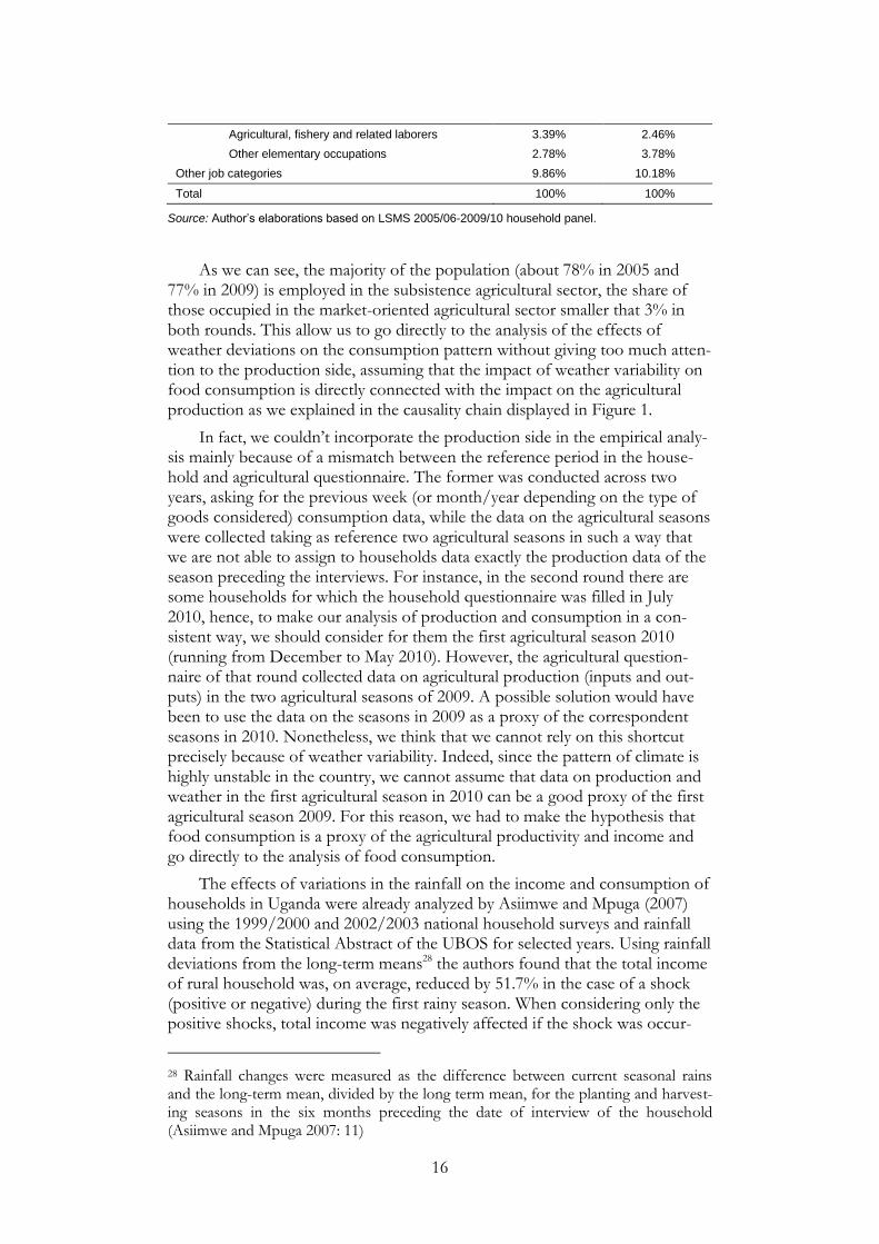
Source: Author’s elaborations based on LSMS 2005/06-2009/10 household panel.

As we can see, the majority of the population (about 78% in 2005 and 77% in 2009) is employed in the subsistence agricultural sector, the share of those occupied in the market-oriented agricultural sector smaller that 3% in both rounds. This allow us to go directly to the analysis of the effects of weather deviations on the consumption pattern without giving too much atten-tion to the production side, assuming that the impact of weather variability on food consumption is directly connected with the impact on the agricultural production as we explained in the causality chain displayed in Figure 1.

In fact, we couldn’t incorporate the production side in the empirical analy-sis mainly because of a mismatch between the reference period in the house-hold and agricultural questionnaire. The former was conducted across two years, asking for the previous week (or month/year depending on the type of goods considered) consumption data, while the data on the agricultural seasons were collected taking as reference two agricultural seasons in such a way that we are not able to assign to households data exactly the production data of the season preceding the interviews. For instance, in the second round there are some households for which the household questionnaire was filled in July 2010, hence, to make our analysis of production and consumption in a con-sistent way, we should consider for them the first agricultural season 2010 (running from December to May 2010). However, the agricultural question-naire of that round collected data on agricultural production (inputs and out-puts) in the two agricultural seasons of 2009. A possible solution would have been to use the data on the seasons in 2009 as a proxy of the correspondent seasons in 2010. Nonetheless, we think that we cannot rely on this shortcut precisely because of weather variability. Indeed, since the pattern of climate is highly unstable in the country, we cannot assume that data on production and weather in the first agricultural season in 2010 can be a good proxy of the first agricultural season 2009. For this reason, we had to make the hypothesis that food consumption is a proxy of the agricultural productivity and income and go directly to the analysis of food consumption.

The effects of variations in the rainfall on the income and consumption of households in Uganda were already analyzed by Asiimwe and Mpuga (2007) using the 1999/2000 and 2002/2003 national household surveys and rainfall data from the Statistical Abstract of the UBOS for selected years. Using rainfall deviations from the long-term means28 the authors found that the total income of rural household was, on average, reduced by 51.7% in the case of a shock (positive or negative) during the first rainy season. When considering only the positive shocks, total income was negatively affected if the shock was occur-

28 Rainfall changes were measured as the difference between current seasonal rains and the long-term mean, divided by the long term mean, for the planting and harvest-ing seasons in the six months preceding the date of interview of the household (Asiimwe and Mpuga 2007: 11)

17

ring in the first planting season or in the second harvesting season (on average, -45.9% and -16.3% respectively). The analysis of the rainfall shocks only on the agricultural income of rural households emphasized the importance of positive shocks in reducing agricultural income if the event was taking place during the second dry season. The 40% average decline indicated by the study in this case could be due to the fact that the shock impeded the realization of the harvest because of the too abundant rains. On the other side, the magnitude and sig-nificance of rainfall shocks on the consumption of rural households were sub-ject to sensible changes. Indeed, when rainfall shocks were not significant or positive and significant but accounting only for 1.2% average increase in con-sumption for a shock in the second dry season. When considering positive shocks only they were found detrimental to consumption (-22.8%) if taking place during the first rainy season, advantageous (+9%) if during the second dry season, non significant otherwise29. This seems to suggest the existence of consumption smoothing strategies (ibid: 18)30. However, a caveat in the analy-sis of the authors could be the fact that rainfall deviations are calculated from the long-term mean including the year considered in the surveys, hence, the estimations could be downward biased in the case those years were particularly different from the other ones. For example, if 1999/2000 was a year of mas-sive rains as compared to the usual rainfall pattern, the long-term mean calcu-lated including the 1999/2000 data would spread the effect of that particular year on the other data, lowering the magnitude of the shock in the analysis. Then, the ability of the method used to capture the effects of the shock on the outcome variable would be compromised.

Concerning the possible coping strategies to mitigate climatic shocks, Hisali et al. (2011) analyzed the determinants of the choice of adaptation (in the words of the author, for a clarification on coping/adapting ability see footnote 2 in the introductory chapter) strategies in response to these particular adverse events using data from the 2005/06 Uganda national household survey (part of which we will use in the analysis in this paper). The authors identified five categories of coping/adaptation strategies: borrowing, modifying the labour supply, decreasing consumption, selling of assets or usage of savings and changing technology or crops. The study suggested that age of the head of the household, credit access, availability of off-farm labour and tenure of land are some of the variables that explain the different choices, depending also on the agro-climatic zone to which households belong. Similarly, Kijima et al. (2006) showed that the coping strategies adopted depend also on the wealth of the household. The authors analyzed the role played by off-farm labour in mitigat-ing the effects of agricultural shocks such as excess or shortage of rainfall (as covariate shocks) and crop and livestock diseases (as idiosyncratic shocks) thanks to a panel of 894 rural households in the period 2003-2005. The results showed an increase in the labour supply only in the case of idiosyncratic shocks and only in the artisanal off-farm labour, especially if the household

29 All the level of significance of the coefficients reported in this paragraph are at con-ventional levels (5 or 1%). 30 the 1999/2000 data would spread the effect of that particular year on the other data, lowering the magnitude of the shock in the analysis. Then, the ability of the method used to capture the effects of the shock on the outcome variable would be compro-mised.

18

had lower asset endowments. Both shocks didn’t have significant impact on self-employed and regular salaried off-farm jobs probably reflecting the diffi-culty in accessing these positions or their more long-term nature. In any case, despite the engagement in more labour of different natures to compensate for the shocks, the extra-income didn’t seem to be enough to compensate the loss of agricultural income, resulting in a higher probability of falling into poverty for the non-poor in 2003. In the study poverty was measured using expendi-tures per adult equivalent, hence, the result just reported implicitly tell us that, in the case analyzed, households that experienced climatic shocks were not able to smooth consumption with the income obtained from secondary jobs under-taken to that purpose. This being said, the discussion of climate and weather variations in the country, through the slowness of the changes in climate and/or the high frequency of weather variations towards a certain pattern, has given some reasons to investigate further in the agricultural activity in the country. Indeed, the words of a farmer interviewed by Magrath (2008: 7), and the awareness of the efforts of the GoU to enhance the development of the agricultural sector in the country promoting its modernization, suggested us to take a look to the production path, hypothesizing that household could have engaged during the years in ex-ante income smoothing strategies such as land extension, crops selection and diversification and the use of fertiliz-ers/pesticides, in a nutshell, technology for adaptation.

Data on production, yields and harvested area for selected crops (the most important in the country as cash and food crops) are reported in Table 5 for selected years, while in Appendix A the reader can find more data. As we can see, the agricultural production in Uganda has generally increased for almost all the crops considered31. In light of the persistency of traditional and basic tech-niques in the agricultural activity32 and of the growing number of studies con-cerning the creation and use of new varieties of heat or drought-resistant seeds33 combined with the increasing technical assistance given by the National Agricultural Advisory Services – NAADS institution, we thought to a modern-ization of agriculture in the country. However, yields remained fairly stable and the studies by Benin et al. (2007) and James (2010) revealed that the govern-ment efforts to modernize agricultural practices were only partially effective. Hence, as the data in Table 5 confirm, the increase in production was mainly due to the progressive extension of the land cultivated. This is also confirmed by the descriptive statistics of our dataset (see Table 6) where the average number of owned parcels of land and their size slightly increased between the two rounds of the panel. We refer to further studies for the analysis of the rea-sons behind this phenomena, for the purpose of our research we only acknowledge that this could have allowed farmers to more effectively diversify

31 Beans and cassava productions were subject to a decline after 2005 because of the spread of particular diseases affecting these cultivations (see for instance Alicai et al. (2007) and Mbanzibwa et al. (2011) on cassava). 32 According to the MAAIF “[t]he hand hoes is still the predominant means for land tillage and other secondary operations in Uganda’s agriculture” {{376 MAAIF 2010/f: 39;}}. 33 See for example Balyejusa Kizito et al. (2007) on cassava, Gibson et al. (2008) on sweet potatoes and Kijima et al. (2008) on rice.

19

the risk from the agricultural activity. We proceed now with the explanation of the empirical strategy.

Table 5 Production, yields and hectares harvested for selected crops in Uganda in selected years.

Production

(1000 Tonnes)

Yield

(Kg/Ha)

Hectares harvested

(1000 Ha)

2000 2005 2010 2000 2005 2010 2000 2005 2010

Banana 610 563 600 4519 3976 4196 135 142 143

Beans 420 478 455 601 577 489 699 828 930

Cassava 4966 5576 5282 12384 14408 12728 401 387 415

Coffee 143 158 162 477 601 600 301 263 270

Groundnuts 139 159 172 699 707 732 199 225 235

Maize 1096 1170 1373 1742 1500 1543 629 780 890

Millet 534 672 850 1391 1600 1809 384 420 470

Plantains 9428 9045 9550 5900 5400 5618 1598 1675 1700

Potatoes 478 585 695 7029 6802 6814 68 86 102

Rice paddy 109 153 218 1514 1500 1558 72 102 140

Sorghum 361 449 500 1289 1527 1515 280 294 330

Soybeans 120 158 175 1132 1097 1129 106 144 155

Sugarcane 1476 2350 2400 73811 69118 60000 20 34 40

Sunflower seeds 79 173 230 1000 1102 1211 79 157 190

Sweet potatoes 2398 2604 2838 4321 4414 4577 555 590 620

Wheat 12 15 22 1714 1667 1720 7 9 13

Source: FAO (2012).

2.3 Model Specification

Basic model

In order to do our analysis of the impact of weather variability on food con-sumption we chose to use a fixed effect model. We explain briefly why, refer-ring for this to the results in Appendix D1-3.

First, we estimated OLS models for the 2005 and 2009 cross sections separately. For both the years the initial estimated equation was

(1)

where is the logarithm of the food consumption expenditures

for household in period when the interview took place, is the

vector of weather deviation variables accounting for deviation from the long-term means (we will elaborate on the construction of these variables in the fol-

lowing chapter), and is the error term. If weather variations have an impact

on food consumption, the coefficients of the weather deviation variables should be negative and significant, since a departure of weather from its usual pattern affects the growth and harvest of the crops, implying (in a subsistence agricultural system) the decrease of food consumption due to the loss of agri-cultural productivity and income. For OLS to be unbiased and consistent, the error term has to be uncorrelated with the explanatory variables, hence, the

20

strict exogeneity34 of weather shocks would allow us to obtain good estimates of how weather variations effects on food consumption. However, this specifi-cation is likely to suffer from omitted variables problem, in other words, there may be other observed and unobserved variables that are correlated with the error term and the weather deviation variables in the explanation of the de-

pendent variable, hence would be biased. For example, we can argue that a households with more adult members is likely to suffer less from losses of in-come and consumption because the sources of income within the unit are more diversified or that households that live in a poorer area are likely to be more affected by weather shocks. Therefore, we modify equation (1) to include a vector of household characteristics (we will discuss them below) able to fur-ther explain the food consumption variable. Similarly, we included a set of variables to take into account unobserved time-invariant factors that can affect the outcome variable to control for unobserved fixed heterogeneity (Wooldridge 2009: 456). In particular, we controlled for the synoptic station to which households were assigned because, although the prevalent rainfall and temperature is bimodal across the country, there are some small variations in the weather variables depending on the different latitude, longitude and alti-tude of the area covered by each synoptic station (the reader may take a look to Table 7 and Appendix B to see the geographical characteristics and the graphi-cal representation of the long-term distribution of monthly rainfall and tem-peratures for each synoptic station35). We also accounted for the region in which the household was settled because each region in the country has differ-ent specific characteristics due different regional poverty dynamics (Deininger 2003, Okurut et al. 2002).

Nevertheless, the results for the separate cross sections models could be driven by some specific weather shocks occurring in the year considered. Hence, we pooled the two cross sections, adding a dummy to account for the change of the year considered (with value one when the year of survey is 2009, zero otherwise). The advantage of having pooled cross section is twofold. Firstly, it increases the size of the sample and secondly, pooled data help to achieve more efficient estimators (especially in the case samples are random). However, pooled cross sections do not allow us to control for differences across households, then, thanks to the nature of the data we had, we could conduct a panel analysis. Panel datasets combine the time series and cross sec-tion dimensions of the observations since every individual/household is fol-lowed across time. In our case we had two periods observations over time for each cross-sectional household in the dataset. The benefits of this feature of panel datasets are multiple. First of all, with longitudinal data we can control for certain individual/household specific unobserved characteristics, allowing for more room to infer causality thanks to the availability of more than one

34 The strict exogeneity assumption states that , in other words, that the explanatory variables are independent from the error term across time. In our case, being the weather shocks likely to be random, once we control for them, there should be no correlation of these variables with the error term, then the hypothesis holds and the OLS estimates should be unbiased and consistent. 35 To a certain extent, we could have controlled for observed synoptic station-specific characteristics, however, accounting for all the agro-climatic characteristics of the lo-cality would have been difficult, hence, the choice of using the fixed effect shortcut.

21

observation per individual/household (Wooldridge 2009: 11). As long as the omitted variables do not change over time, we can obtain unbiased estimators using a differenced specification of the model, provided that the strict exoge-neity assumption conditional on unobserved variables holds36. Also, when the periods are two, fixed effect estimators and first difference estimators coincide, as in our case (ibid: 487). Second, as Baltagi (1995: 5) states: “more informative data, more variability, less collinearity among variables, more degrees of free-dom and more efficiency” are some advantages of this methodology together with the higher suitability for the study of the dynamics of change in the vari-able of interest, accounting also for behavioural changes (Gujarati and Porter 2009: 637). If the panel is unbalanced (for some individuals/households there are missing years, this phenomena called attrition), “one degree of freedom is lost for every cross-sectional observation due to time-demeaning”, however, a fixed effect estimation would “allow attrition to be correlated with [...] the un-observed effect (we will deal with the attrition problem concerning our dataset in Appendix C). Note that if the unobserved effects were not correlated with the error term, a random effects model would be better in terms of consistency and efficiency of the parameters estimated (the latter property is lowered in the case of fixed effects models due to the loss of some information). However, the Hausman test supports the use of a fixed effects model (p-value 0.000 im-plies that the null hypothesis of non-systematic difference in the coefficients of the two models is rejected). Hence we estimate the following model

(2)

where is the logarithm of the food consumption expenditures for

the household h assigned to the synoptic station s in year t, is a vec-

tor describing the weather deviations from the respective long term means

while is a vector of household specific characteristics. , and are

the synoptic station, region and time fixed effects while is the error

term. This model is expected to have consistent estimates of the effects of weather variability on food consumption expenditures, provided that the un-observed time-invariant households, synoptic stations and regions (and all oth-er fixed characteristics in time) in the dataset are not correlated to the idiosyn-cratic error.

Choice of variables

The decision about the households specific characteristics variables to take into account in the analysis is largely based on the study by Bird and Shinyekwa (2005) on poverty in Uganda, which combines households surveys and partici-patory studies, and on the general understanding of the poverty dynamics in a poor rural developing country.

36 The strict exogeneity assumption conditional on the unobserved effects states that

. In other words, this assumption states that, provided we controlled

for the unobserved effects , “there is no correlation between the and the re-

maining idiosyncratic error, , for all and ” (Woolridge 2009: 479). Using first difference estimators, since the procedure leaves out the time invariant unobserved

effects, reduces the assumption to , for consistency. Hence estimators will be unbiased.

22

The sex of the head of the household was included because in the context we are analyzing female-headed households are likely to be poorer (lower con-sumption) due to many reasons. For example, lower possibility to access land and other assets (even in the case of separation or divorce) due to the fact that generally property rights are retained by the men, makes female-headed house-holds more vulnerable. Moreover, in districts affected by conflict, the female-headed households could be in this role due to the death of the husband/male-head. The sudden loss of the income of the male-head, in connection with the likely transfer of land rights to other male individuals, could affect the ability of the newly female-headed household (ibid: 69). Hence, we expect this variable to have a negative coefficient on the food consumption variable. Similarly, the age of the head of the household was included because it is likely that older heads enjoy higher ability to earn (and then more food consumption possibili-ties for the household as a whole). Then, we generally expect the coefficient of the variable to be positive. However, it is likely that after a certain age older heads constitute a less important source of income in the unit (for example in the case of retirement), then we introduced the head age squared variable to account for decreasing marginal returns to food consumption (hence the coef-ficient on this variable should be negative).

Household size and demographic composition should be very important in determining the level of food consumption. Indeed, since nutrition is a basic need, we can expect the sign of the coefficient of the variable accounting for the size of the household to be positive (more members require more food consumption expenditures). When it comes to the analysis of the composition of the household, we can argue that the signs and magnitudes of the coeffi-cients will depend on the prevalent behavioral norms in the country. In other words, if priority is given to adults as income-earners instead that to children (since they do not contribute to the generation of resources) we will expect bigger coefficients for older cohorts. On the other side, the awareness that children need better nutrition in order to become strong (and productive) adults could be reflected in higher coefficients for the younger cohorts. In any case the signs are expected to be positive for the reasons aforementioned. Moreover, in light of the young structure of the population in Uganda (World Bank. 2011a), we can argue that larger coefficients should be found for the younger cohorts.

The ownership of the house seemed to be fairly common in the country (see Table 6) and it is generally considered a sign of wealth, increasing as the size of the house in terms of room is growing. Then, we included both the var-iables in the analysis and we expect a positive sign for both the coefficients. The ownership of land in terms of number of parcels and size of the parcels owned was introduced to account for possibility to diversify the risk from weather and as a sign of wealth respectively. Hence, we suppose that the signs of both the coefficients of these variables will be positive. However, we intro-duced these variables only in some specifications because for them we had some missing observations. Even more problematic for the missing observa-tions were the variables accounting for the education of the head of the house-hold. More educated heads are likely to have access to better paid jobs or to have a better knowledge of the most recent agricultural techniques to obtain a higher agricultural income and a higher food consumption, hence the high

23

probability to have a positive coefficient. These variables were introduced only in secondary specifications as the variables on land ownership.

Besides the household characteristics, we had to take into account for the season when the household was interviewed. Indeed, as suggested by Behrman et al. (1997: 189) in the absence of complete markets and/or perfect insurance, consumption is driven by the expectations on the income realized in the har-vesting season, implying food consumption seasonality (especially in the case of subsistence agriculture). In other words, if the household was interviewed during one of the rainy/planting seasons, it is likely that its consumption is lower because it is relying on the harvest or on the income received from the selling of the crop harvested in the previous dry season. On the contrary, a household interviewed in the dry season is likely to be in the process of receiv-ing or has already received the revenues of the selling of the just harvested crops, hence a higher consumption, especially of food when the agricultural activity is for subsistence.

We will discuss the weather deviation variables in the following chapter, here we just want to make clear that their calculation is made with reference to the long term-means calculated in the period 1960-90 (1980-2010) and on a seasonal (dry/rainy) basis. We will first estimate the models for the rainfall de-viations only, then for rainfall and number of rainy days together, after for the temperatures deviation only, and finally for all the weather deviations together.

Persistency

The work of Dercon (2004) on shocks in Ethiopia and the relationship be-tween the subsistence nature of the agricultural activity and the likely seasonal pattern of the food consumption, inspired us to investigate the persistency of weather deviation effects. Then, in order to check for the persistency of shocks occurring in the second season back in time on the current food consumption,

we estimated equation (2) adding the persistency term

(3)

If weather variations have persistent negative effects on food consump-

tion, should be negative and significant.

Heterogeneity of impacts

According to Skoufias (2011: 20), it may be that the average effect of weather variations on the outcome variable is masking differences of impacts between households with different welfare levels depending on the ownership of crucial asset such as the house where the household lives or land. Hence, we estimated equations (2) introducing an interaction term

(4)

The term incorporates the specific household feature that we think

important in determining different impacts of weather variations on food con-

sumption. Therefore, measures the impact of weather variations independ-

ently of particular households characteristics while measures the

24

impact of weather deviations on those households with the specific characteris-tic considered (house or land ownership).

We proceed now with the preliminary analysis of the data at hand and the definition of the weather deviation variables.

25

Chapter 3 The Data

3.1 Household data

The analysis of the impact of weather variability on food consumption is con-ducted using a panel dataset made publicly available by the World Bank Living Standard Measurement Study (LSMS) website. The baseline survey comes from the Uganda National Household Survey (UNHS) conducted in 2005/2006. Within this, 3,123 households distributed over 322 enumeration areas (EAs) over the 783 EAs visited by the UNHS were selected by the Uganda National Panel Survey (UNPS) to conduct the interviews in 2009/2010. In the panel a household “was defined as a group of people who have normally been living and eating their meals together for at least 6 of the 12 months preceding the interview” (UBOS 2010: 8). In the 2009/2010 follow-up also guests or visitors and members abroad or overseas were surveyed but, for the purpose of our analysis we decided to consider only usual and regular members. About 10% of the households were selected for tracking in 2005/06 in order to take into ac-count in 2009/10 of split-off households for representativeness. However, for the purpose of comparison of changes between the surveys of the panel we will not take into account of the split-off households. In the analysis we will consider only those households that were reported as rural households in both the rounds of interview (2,248 in total) since, as we made clear in the previous sections, urban households differ from rural households for the level of vul-nerability of their income and consumption to weather variation37. The dataset contains information on the socioeconomic status of the households, with a detailed module on food and non-food (non-durable and semi-durable) con-sumption expenditures. Descriptive statistics for the household variables of interest are reported in Table 6.

The panel is unbalanced (11.5% attrition rate), hence, we need to check if the 258 households that dropped out of the 2005/06 sample in 2009/10 are systematically different from those who remained in it. In this case the dataset representativeness of the original population would be undermined, the results of the empirical analysis based only on those households that were in both rounds. Therefore, these results might be critically influenced by the attrition bias. If the attrition is random nothing has to be done to correct for it, while in the opposite case two procedures can be applied to correct for this problem in order to avoid coefficients biases. The first is the use of inverse probability weights while the second is the estimation of a Heckman type selectivity model (Baulch and Quisumbing 2011). The discussion of the attrition problem in the data analyzed is dealt with in Appendix C were we detected the presence of non-random attrition and we estimated inverse probability weights to correct

37 In fact, it is likely that urban households derive their income from activities different from the agricultural one, hence, for them the chain of causality explained in Figure 1 is less likely to hold. Weather deviations may have an impact on urban households food consumption through agricultural output prices but this analysis is beyond our concerns.

26

the data and give more importance to those observations that had the same characteristics of the “droppers” in the second round. With this procedure the bias in the estimations should be reduced. However, the inverse probability weights that we calculated didn’t change sensibly the weight of the different households in the panel (the mean value of the weights calculated was 1.0185). Moreover, standard error of the models estimated were fairly robust to both the representativeness and attrition weights. Nevertheless, we decided to report the results of the models with the attrition weights because we are also con-cerned with the magnitude of the coefficients.

To conclude, since the food consumption data were collected on the basis of a week recall, we made the variable monthly, corrected for inflation (monthly in 2005, and monthly using the base year 2005 for the 2009 data) and we took the logarithm of it38. In Table 6 we report however the level instead of the logarithm of the monthly food consumption variable in Ugandan Shillings (UGX) because we think in this way it is easier to understand the level of eco-nomic welfare in the country.

38 Monthly inflation rates for food items came from the Bank of Uganda statistics (BOU. 2012).

27

Table 6 Descriptive statistics of selected variables for rural households in Uganda.

2005/06 2009/10

Variable Mean St. Dev Mean St. Dev

Month survey 8 1.5782 7 3.5884

Year survey 2005 0.4793 2009 0.4805

Dummy season (Rainy=1) 0.4225 0.4941 0.4962 0.5001

Sex Head HH (Female=1) 0.2656 0.4417 0.2844 0.4513

Age Head HH 42.9057 15.6442 46.9789 15.1369

Education head of the household°

(1) No education 0.0094 0.0966 0.0234 0.1514

(2) Some/completed primary 0.7394 0.4391 0.7334 0.4423

(3) Post-primary specialization 0.0371 0.1890 0.0315 0.1747

(4) Some/completed junior high 0.0200 0.1400 0.0221 0.1471

(5) Some/completed secondary 0.1553 0.3623 0.0221 0.3559

(6) Post secondary specialization 0.0347 0.1831 0.1487 0.1851

(7) Degree or above 0.0041 0.0641 0.0053 0.0730

Household size 5.5338 3.0451 6.1779 3.1325

Share of males 0-5 0.1023 0.1347 0.0951 0.1265

Share of males 6-11 0.0798 0.1169 0.0911 0.1165

Share of males 12-17 0.0683 0.1181 0.0863 0.1241

Share of males 18-64 0.2236 0.2280 0.1984 0.1983

Share of males >65 0.0245 0.1154 0.0258 0.1133

Share of females 0-5 0.1041 0.1393 0.0923 0.1244

Share of females 6-11 0.0794 0.1126 0.0909 0.1176

Share of females 12-17 0.0663 0.1133 0.0818 0.1213

Share of females 18-64 0.2235 0.1672 0.2087 0.1479

Share of females >65 0.0283 0.1250 0.0298 0.1225

Own house (Yes=1) 0.8794 0.3257 0.9140 0.2805

No. Rooms 4.0321 2.3635 2.9552 1.7326

Owned parcels number° 1.6677 1.4910 1.8898 1.4281

Owned parcels size (Hectares)° 3.5447 19.2189 3.8293 20.0519

Food consumption (monthly, adj.)° 82,027.72 64,446.99 84,053.09 64,963.12

Region 1 – Central 0.2464 0.4310 0.2417 0.4282

Region 2 – Eastern 0.2513 0.4339 0.2553 0.4361

Region 3 – Northern 0.2473 0.4316 0.2573 0.4372

Region 4 – Western 0.2549 0.4359 0.2457 0.4306

N 2248 1990

Source: Author’s elaborations based on LSMS 2005/06-2009/10 household panel.

Note: 1 USD=1,780 UGX in 2005. HH stands for “household”.

° The number of observations for the education of head of the household variables is 1700 for the year 2005/06 and 1493 for 2009/10. Similarly, the number of observations for the variables accounting for the owned parcels number and size is 2010 in 2005/06 and 1879 in 2009/10. Finally, 6 and 25 observations were missing for the food consumption variable in 2005/06 and 2009/10 respectively.

28

3.2 Weather data

The climate data are given by the Uganda Ministry of Water and Environment, Department of Meteorology (UDOM). The UDOM has registered daily weather data about precipitation, maximum and minimum temperatures for 13 synoptic stations located throughout the country (Appendix H reports the map of the country showing where the synoptic stations are located). The long term averages for the rainfall data are comprehensive of the period 1960-1990 while for temperatures they are calculated on the 1980-2010 time frame. Table 7 shows the distribution of the synoptic stations in the country while in Appen-dix B the reader can find the figures with the monthly average long term means of rainfall and maximum and minimum temperatures for every synoptic sta-tion.

Table 7 Distribution of synoptic stations across Uganda.

Synoptic Station

Region Longitude Latitude Altitude (meters)

Region Area (sq-Km)

Arua

Northern

30.917 3.05 1280

85,391.7 Gulu 32.283 2.783 1105

Kitgum 32.883 3.3 940

Lira 32.933 2.317 1110

Soroti

Eastern

33.617 1.717 1132

39,478.8 Tororo 34.167 0.683 1170

Jinja 33.183 0.45 1175

Kampala Kampala 32.633 0.25 1200 197.0

Entebbe Central w/o Kampala 32.45 0.05 1155 61206.3

Mbarara

Western

30.683 -0.6 1420

55,276.5 Masindi 31.717 1.683 1147

Kasese 30.1 0.183 691

Kabale 29.983 -1.25 1869

Source: Author’s elaborations based on UDOM weather data.

Households and individual members were assigned data on the synoptic station on the basis of the proximity to the district of residence39. From the weather data we calculated the average seasonal rainfall millimetres, number of rainy days and maximum and minimum temperatures for the two seasons pre-ceding the day of interview in order to take into account for the effects of weather variability on the reported food consumption. We calculated the devia-tions of these averages from the respective seasonal long term means, follow-ing the procedure of Paxson (1992) except for the fact that we used the 1960-1990 long term means instead of the means calculated over all the years. Our choice, similarly to Skoufias et al. (2011), is to exclude more recent years that may have incorporated the impact of climatic change on the country. Hence, we assigned two rainfall and temperature variables for each household, one pertaining to the previous dry (harvesting) season and one pertaining to the previous rainy (planting) season. Since the households were interviewed in dif-

39 The average distance is 32.5 Km with a standard deviation of 22.4 Km.

29

ferent months, they were assigned different rainfall deviations. In the case the household was interviewed in the first dry season of year t, it was assigned firstly the deviations calculated in the second rainy season of year t-1 and sec-ondly the deviations calculated in the second dry season of t-1, to check for persistence in the weather shocks (analogously to the analysis of Dercon (2004)). If the household was interviewed in the first rainy season of year t, it was assigned firstly the deviations calculated in the first dry season of year t and secondly the deviations calculated in the second rainy season of t-1. This pro-cedure can be made clearer looking to Figure 2 and 3. For example, an house-hold interviewed in June 2005 was assigned firstly the March-April-May 2005 deviations and secondly the December-January-February 2004/05 deviations.

Figure 2 Agricultural cycle in Uganda.

Source: Author’s elaborations based on LSMS 2005/06-2009/10 household panel and Asiimwe and Mpuga (2007).

Note: In light grey we can see the month in which the interviews were conducted.

Figure 3 Example of the mechanism of assignment of weather deviations.

Source: Author’s elaborations based on LSMS 2005/06-2009/10 household panel and Asiimwe and Mpuga (2007).

Weather deviation descriptive statistics for the two years are reported in Table 8, while from Table 7 we recall that between 40 and 50% of the house-holds were interviewed during one of the two rainy seasons in the year consid-ered. On average in the country there is a good amount of variability in the

30

seasonal rainfall precipitations towards a wetter climate. In fact, the means of the variables for the deviations of millimetres of rain from the long-term mean both in the first and second previous period in both the rounds (except in 2005/06) are positive and increasing between the two periods.

On the other side, temperatures increased, especially when we look to the minimum ones, that on average increased by one degree, in some places even to almost five more degrees.

Table 8 Descriptive statistics of weather deviations variables.

2005/06

Variable Mean St. D. Min Max

Rain deviation (-1) 4.1195 30.7680 -69.6 62.6

No. rainy days dev. (-1) 0.1876 1.8244 -4 4

Max temp. dev. (-1) 0.6070 1.1620 -2.4 4.6

Min temp. dev. (-1) 1.0359 1.0774 -0.7 4.7

Rain deviation (-2) -5.3511 23.4353 -69.6 67.1

No. rainy days dev. (-2) -0.4786 1.8526 -4 5

Max temp. dev. (-2) 0.9499 1.2333 -2.2 4.8

Min temp. dev. (-2) 1.0957 1.0855 -0.7 4.7

N 2248

2009/10

Variable Mean St. Dv. Min Max

Rain deviation (-1) 9.6531 34.3391 -68.5 110.2

No. rainy days dev. (-1) 0.5583 2.2847 -5 5

Max temp. dev. (-1) 0.3897 0.9736 -3 3

Min temp. dev. (-1) 0.8866 0.9038 -0.8 3.7

Rain deviation (-2) 1.6347 38.2037 -68.5 110.2

No. rainy days dev. (-2) 0.2251 2.3028 -5 5

Max temp. dev. (-2) 0.3919 1.0071 -3 3

Min temp. dev. (-2) 0.8528 0.9392 -0.5 3.7

N 1990

Source: Author’s elaborations based on UDOM weather data.

We will control for regional effects because, despite the fact that the prevalent distribution of rains is bimodal, we are aware that the northern re-gion has an unimodal distribution with a unique rainy season lasting from March to August and dry season from September to February. However, our decision to use the two weather variables also in this region is still a valid choice since the subdivision corresponds to the point of peak of the two sea-sons, hence, with this repartition we can track from the onset of the rainy sea-son to its peak and the same for the dry season.

31

Chapter 4 Results

4.1 Average effects of weather deviations on food consumption

The results for the impact of weather deviations on food consumption are given in the following Tables and in the Appendixes. Negative and significant coefficients will mean that weather deviations, either negative or positive, from the long-term mean can have a negative impact on the consumption of food items. We will discuss first the impact of rainfall deviations, then the joint im-pact of rainfall and number of rainy days, after the effect of temperatures varia-tions only and finally the effect of all the weather deviations combined on the outcome variable. Moreover, we will also check for the persistency of weather deviations shocks in the second season back in time with respect to the date of interview. The control variables for the odd numbered specifications in the tables are sex and age (also squared) of the head of the household, size and demographic composition of the household, ownership and size of the house, a dummy for the season of interview (taking value one when the season is the rainy) and a year dummy (taking value one when the year is 2009). The even numbered specifications also include ownership of land (number and size of parcels) and education of the head of the household. We chose to include these variables only after because for them (especially for the education vari-ables) we had many missing observations that could have resulted in biased estimations.

As we mentioned in the model specification section, estimating the model using only the 2005/06 or 2009/10 cross sections without any control variable would bring us biased estimates due to omitted observed variables and the likely correlation of the error term with time-invariant unobserved factors. In fact, when we look at the results in Appendix D1 and D2 for the specifications a-d, we find that no weather deviation variables except temperatures have a significant impact on food consumption in 2005/06 while in 2009/10 only minimum temperatures and number of rainy days deviations are significant. Moreover, when it comes to the magnitude of these coefficients it seems that weather variations also have a positive impact on our outcome variable, con-trary to our expectations40. The results for the pooled cross sections without control variables are similar, suggesting that the estimations for the individual cross-sections were not driven by particular weather phenomena in the years considered. Therefore, we estimated the separate and pooled cross-sections models including some observed and unobserved fixed households characteris-

40 We would be more keen to accept positive signs if we knew that weather variations were small. In fact, we can argue that, for example, slightly more rains can have a posi-tive impact during the planting season, allowing for better yields in the harvesting sea-son and ultimately in a higher agricultural income and food consumption. However, we know from the descriptive statistics of the weather variables that their variability is quite important in the sample, then, ceteris paribus the expectation of negative signs should be confirmed.

32

tics41 (see Appendix D1-3, specifications e-h). The signs of some of the weather variables became negative and temperatures gained significance in the 2009/10 models. The pooled cross-sections estimations instead highlighted the deviation of the number of rainy days variable both when considered alone and together with the other weather deviations. Nevertheless, we emphasized the advantages of panel estimations and for the aforementioned reasons here we discuss more in detail only the results of this particular methodology.

Rainfall, rainy days and temperatures deviations separately

Rainfall deviations seem to have a small but significant impact on food con-sumption. Indeed, on average and controlling for households demographic and economic characteristics, we have that 10 millimetres of rain deviation from the long-term mean lower the food consumption by 0.8%, with a 5% level of significance. When we control for the number and size of the parcels of land owned by the household and for the education of the head of the household, we have that the impact on food consumption becomes significant at 1% and it is higher. The magnitude in this case is on average 1.2% for 10 millimetres deviation, suggesting that the ownership of land allows the households to slightly insure from potential losses. In particular, if we look to Appendix E in which we reported the complete results, we can see that what really matters is number of parcels owned (significant at 1% while the size of the land and the education variables are positive but not significant). In fact, we can argue that if the household owns more parcels, it can diversify the risk from weather variations choosing to cultivate different crops or crop mixes in every parcel42.

When we combine the rainfall with the number of rainy days deviations, we can see that the real shock is given by the change in the number of rainy days, the coefficients on rainfall decreasing and losing significance. This result confirms what was described by the interviewees in the OXFAM report (Ma-grath 2008) and by the time series analysis of Mubiru (2012), namely, the fact that even if on average the millimetres of rain received during the season are the same as they used to be, the problem arises with their distribution. In other words, for example during the rainy season March to May, the rain comes heavily concentrated in fewer days instead of coming every day in little quanti-ties in such a way that the crops receive the daily (and seasonal) quantity of wa-ter that they need to grow43. In (3) we can see that on average, the effect of one day deviation in the number of rainy days decreases food consumption by 1.36% with a 10% level of significance, while a deviation in rainfall millimetres

41 The observed households characteristics included in the specifications were the sex, age and age squared of the head of the household, the size and demographical compo-sition of the unit, ownership of the house and number of rooms and a dummy for the season of interview. A dummy for the year was added in the case of pooled cross-section. 42 It may also be that diversification is brought about by the different location of the parcels in the country. In this case, shocks experienced by the cultivations in every parcels will be different. 43 Here we recall the already cited work by Otegui et al. (1995) in which the authors proved that if maize (that is one of the most cultivated crops in Uganda) receives too low amount of water particularly at the silking (flowering) phase the yields will be af-fected, despite the water and pollination received after are in the right amount.

33

seems to not affect the outcome variable significantly anymore. Controlling for land and head education makes the weather deviation variables not significant, suggesting again for some kind of smoothing strategies due to different land management when the land is owned (again, the number of owned parcels has a positive coefficient, significant at 1%, the size of the parcels and the educa-tion of the head of the household being positive but not significant).

Table 9 Econometric results, fixed effect estimations.

ln food consumption expenditures

Variable (1) (2) (3) (4) (5) (6)

Rainfall (-1) -0.0008** -0.0012*** -0.0004 -0.0008

(0.0003) (0.0004) (0.0004) (0.0005)

Rainy days (-1) -0.0136* -0.0096

(0.0074) (0.0090)

Max temp. (-1) 0.0086 0.0048

(0.0141) (0.0170)

Min temp. (-1) 0.0030 -0.0277

(0.0202) (0.0227)

Dummy season (R=1)

-0.0738*** -0.0685** -0.0795*** -0.0724*** -0.0818*** -0.0736**

(0.0235) (0.0278) (0.0237) (0.0278) (0.0248) (0.0287)

Constant 9.497*** 8.390*** 9.483*** 8.368*** 9.481*** 8.418***

(0.291) (0.530) (0.291) (0.533) (0.290) (0.539)

N 4,137 2,937 4,137 2,937 4,137 2,937

NH 2,213 1,694 2,213 1,694 2,213 1,694

R2 within 0.137 0.166 0.139 0.167 0.135 0.162

Source: Author’s elaborations based on LSMS 2005/06-2009/10 household panel and UDOM weather data.

Note: The control variables included in the odd numbered specifications are: sex and age (also squared) of the head of the household, size and demographic composition of the household, ownership of the house and number of rooms, year dummy. The even numbered specifications include also the education of the head of the household and the number and size of the owned parcels of land. Robust standard errors in parenthesis. *, **, *** stand for level of significance at 10, 5 and 1% respectively.

Temperature deviations alone do not seem to affect food consumption significantly, if so, they would have positive impacts on food consumption, a result that doesn’t seem to be very much in line with the understanding of the crops cycle.

Consistently with the subsistence nature of the agricultural activity, the dummy capturing the season when the household was interviewed is always fairly large, negative and significant at conventional levels, depending on the fact that we add more control variables to the specifications. This result seems to account for a seasonal pattern in the food consumption for households in Uganda. In other words, on average if the household was interviewed during the rainy season, the food consumption is likely to be lower by 7.38% (6.85%) when we consider the rainfall deviations only, 7.95% (7.24%) when we con-sider also the number of rainy days, and 8.18% (7.36%) in case of temperature deviations only, with a 1% (5%) level of significance. As we stated, this result is not surprising if we consider the fact that the bulk of the households members are employed in the agricultural sector for subsistence (see Table 4). In fact, being the rainy season the season of planting, if the household was surveyed during it, it means that it would have been still relying on the harvest of the

34

previous (dry) season- or eventually on the revenues from its sale on the mar-kets in the case of a surplus harvesting season- for its own consumption. On the other side, if the household was interviewed during a dry/harvesting season it would have been in the position of having just collected the harvest, hence, it is likely to have a higher food consumption. In Appendix F and G we explored more the seasonality pattern of food consumption, to understand the magni-tude of the phenomena, in light of the fact that some authors claimed the im-portance of exploring this aspect often overlooked (Chambers 2009, Gill 1991).

Persistency

We added to the analysis that we discussed before the weather deviation re-lated to the second season back in time with respect to the season when the household was interviewed in order to check for the persistence of weather shocks on the food consumption of rural households in Uganda.

When we account for rainfall deviations only, we can see that on average, 10 millimetres deviation in rainfall in the second preceding season will decrease food consumption by 0.7% with a 5% level of significance, the same magni-tude and level of significance of a shock in the (closer) previous season. Similar effects are reported in the case we add as control variables the land ownership (size and number of parcels) and the head of the household level of education (-1.1 and -0.9% in the first and second previous season respectively, significant at 1% for 10 millimetres rainfall deviation). When considering also the devia-tions for the number of rainy days, we can see again the importance of this variable as the real shock to the households (lowering the impact of rainfall deviations), but the significance of this shock is limited to the first previous season (-1.45% for one day deviation with 10% level of significance in (9)). In-cluding other control variables, however, makes both rainfall and number of rainy days insignificant. In the same way as in the discussion above, the dummy variable for the season of interview is highly significant and replicating the sea-sonal pattern of food consumption.

As far as temperature deviations is concerned, we found that on average the deviations that adversely affect food consumption, and in a persistent manner, are those occurring in the minimum temperatures. Indeed, a one de-gree deviation in minimum temperatures in the previous period lowers food consumption by 4.63% with a 10% level of significance while, if this change happens in the second season back in time, it decreases consumption by 8.12% with the highest level of significance. This result can easily be understood if we remember that the specification is taking as reference a household interviewed in the dry season. In fact, going back two seasons, it means that the reference household has experienced a warmer dry season, probably losing the harvest and in the current dry season it is probably still relying on the small harvest of that period for the consumption, waiting to realize the current one, or trying to limit its consumption in order to build up stocks for the coming period (for a deeper discussion of seasonal effects of shocks see Appendix F and G).

35

Table 10 Econometric results, fixed effect estimations. Persistency checks.

ln food consumption expenditures

Variable (7) (8) (9) (10) (11) (12)

Rainfall (-1) -0.0007** -0.0011*** -0.0002 -0.0006

(0.0003) (0.0004) (0.0004) (0.0005)

Rainy days (-1) -0.0145* -0.0115

(0.0075) (0.0092)

Rainfall (-2) -0.0007** -0.0009*** -0.0006 -0.0005

(0.0004) (0.0004) (0.0005) (0.0005)

Rainy days (-2) -0.0037 -0.0092

(0.0079) (0.0095)

Max temp. (-1) -0.0077 -0.0195

(0.0155) (0.0184)

Min temp. (-1) 0.0463* 0.0086

(0.0259) (0.0284)

Max temp. (-2) 0.0165 0.0419**

(0.0142) (0.0175)

Min temp. (-2) -0.0812*** -0.0654**

(0.0303) (0.0330)

Dummy season (R=1)

-0.0765*** -0.0746*** -0.0809*** -0.0753*** -0.0925*** -0.0586*

(0.0236) (0.0280) (0.0241) (0.0283) (0.0279) (0.0326)

Constant 9.489*** 8.373*** 9.468*** 8.342*** 9.528*** 8.389***

(0.291) (0.528) (0.292) (0.528) (0.293) (0.539)

N 4,137 2,937 4,137 2,937 4,137 2,937

NH 2,213 1,169 2,213 1,169 2,213 1,169

R2 within 0.139 0.169 0.141 0.170 0.138 0.169

Source: Author’s elaborations based on LSMS 2005/06-2009/10 household panel and UDOM weather data.

Note: The control variables included in the odd numbered specifications are: sex and age (also squared) of the head of the household, size and demographic composition of the household, ownership of the house and number of rooms, year dummy. The even numbered specifications include also the education of the head of the household and the number and size of the owned parcels of land. Robust standard errors in parenthesis. *, **, *** stand for level of significance at 10, 5 and 1% respectively.

When we account for ownership of land and education of the head of the household it seems that only the temperatures in the second season back in time affect food consumption. In fact, a one degree increase in the minimum temperatures in the second season back in time seems to reduce food con-sumption by 6.54% (with 5% level of significance) while the same variation in maximum temperatures seems to increase food consumption by 4.19% (sig-nificant at 5%). This result could be influenced either by specific crops tem-perature requirements during the harvesting season or by the fact that in this specification we lost many observations due to amount of missing values for some of the variables that we included, hence, any interpretation with this re-spect must be taken with caution.

All weather deviation and persistency

We consider now in Table 11 all the weather deviations together since we know that the results of the agricultural activity are a combination of all the weather indicators: millimetres of rain, number of rainy days and minimum and

36

maximum temperatures. In specifications (13) and (14) we have the results for the previous season deviations only while in (15) and (16) we check also for the persistency of weather deviation effects from the two seasons before the inter-view.

Table 11 Econometric results, fixed effect estimations. All weather deviations and persistency.

ln food consumption expenditures

Variable (13) (14) (15) (16)

Rainfall (-1) -0.0004 -0.0008 -0.0002 -0.0006

(0.0004) (0.0005) (0.0004) (0.0005)

Rainy days (-1) -0.0145* -0.0118 -0.0140* -0.0154

(0.0075) (0.0092) (0.0078) (0.00975)

Rainfall (-2) -0.0239 -0.0007

(0.0163) (0.0006)

Rainy days (-2) 0.0280 0.0172

(0.0269) (0.0098)

Max temp. (-1) -0.0073 -0.0146 -0.0007 -0.0418**

(0.0148) (0.0179) (0.0005) (0.0192)

Min temp. (-1) 0.0006 -0.0309 -0.0009 -0.0177

(0.0204) (0.0228) (0.0081) (0.0300)

Max temp. (-2) 0.0117 0.0378*

(0.0157) (0.0199)

Min temp. (-2) -0.0654** -0.0424

(0.0316) (0.0349)

Dummy seas .(R=1) -0.0763*** -0.0632** -0.0860*** -0.0470

(0.0249) (0.0291) (0.0287) (0.0350)

Constant 9.486*** 8.421*** 9.525*** 8.383***

(0.291) (0.535) (0.295) (0.534)

N 4,137 2,937 4,137 2,937

NH 2,213 1,694 2,213 1,694

R2 within 0.139 0.168 0.143 0.177

Source: Author’s elaborations based on LSMS 2005/06-2009/10 household panel and UDOM weather data.

Note: The control variables included in the odd numbered specifications are: sex and age (also squared) of the head of the household, size and demographic composition of the household, ownership of the house and number of rooms, year dummy. The even numbered specifications include also the education of the head of the household and the number and size of the owned parcels of land. Robust standard errors in parenthesis. *, **, *** stand for level of significance at 10, 5 and 1% respectively.

In (13) we can see again that the weather indicator that really matters in af-fecting the consumption of food is the one that concerns the number of rainy days: on average, food consumption decreases by 1.45% for one day deviation (negative or positive) from the long-term mean with a 10% level of signifi-cance). When considering the land ownership and the education of the house-hold head, all the weather variables become insignificant suggesting for a cer-tain insurance mechanism induced by these variables. We will explore this in the following sections.

Persistency of deviations seems to hold for minimum temperatures. In-deed, this variable would cause a reduction of food consumption by 6.54% for

37

a one degree deviation (significant at 10%). A possible reason is that, consider-ing that the reference household was interviewed in the dry season, the second season back in time is again a dry season, then, an increase in the minimum temperatures could cause the loss of the harvest because higher minimum temperatures do not allow the right level of humidity for the crops not to be damaged during the harvesting phase. On the other side, when we include land and head education we have that only maximum temperatures seem to affect food consumption. However, their effects are mixed. In fact, on average maximum temperature seem to have a negative impact if occurring in the first season back in time (-4.18% at 5% level of significance for one degree devia-tion) while if the same change occur in the second previous season, the impact on food consumption is positive (+3.78 at 10% significance level for one de-gree deviation). Again we have to warn the reader from possible problems de-riving from missing data or clarify that a better study of the crops characteris-tics could shed some light on the different effects of minimum and maximum temperatures during the harvesting season.

Household socio-demographic variables

Households socio-demographic characteristics proved to be very important in influencing the amount of food consumption. Indeed, as we can see in Appen-dix E where we reported the complete results for specifications (1) to (16), the household size is always positive and significant at 1% level, indicating that when the households has more members, its food consumption is higher. For example, on average an additional member increases consumption by 6 to 6.76% depending on the type of weather deviation and other control variables considered. The magnitude and level of significance of the variables accounting for the shares of male and female members divided by groups of age show that not only the size but also the actual composition of the household have an in-fluence on the amount of food consumed overall. For instance, a 1% increase in the share of girls aged 6 to 11 brings, on average, an increase in food con-sumption by 0.81 to 1.89% with a 1% level of significance (the reference cate-gory here is the share of female members more than 65 years old). The latter figure is reported when we control for ownership of land, suggesting that when the household is wealthier, it gives more attention to the nutrition of female children in primary schooling age.

The sex of the head of the household has always negative sign as expected, suggesting the fact that female-headed households can afford lower food con-sumption with respect of their male-headed counterparts. However, this vari-able becomes significant only when we control for land ownership, highlight-ing the fact that property rights in Uganda are generally in the hands of men. Again on the head of the household, it seems that older heads have a positive impact on food consumption with decreasing marginal returns, again confirm-ing our expectations.

4.2 Heterogeneity of impacts

As we argued in the model specification section, it may be that the average ef-fect of weather variations on the outcome variable is masking differences of impacts between households with different welfare levels depending on the

38

ownership of crucial assets such as the house or the land. Hence, we estimated our model introducing an interaction term to account for the impact of shocks when the household owns the house, depending on the number of parcels owned and depending on the size of the land owned. The estimations account-ing for land are conducted also in light of our analysis on the agricultural pro-duction where we emphasized an increase during the years of both the number and size of parcels of land cultivated. Here we report only the results for the specifications that consider the rainfall millimetres deviation alone since in all the other specifications the F-test for the joint significant of the weather vari-ables with the interaction terms were rejecting the null hypothesis of joint sig-nificance.

Table 12 Econometric results, fixed effect estimations. All weather deviations and persistency.

ln food consumption expenditures

Variable (17) (18) (19)

Rainfall (-1) 0.0026 -0.0005 -0.00107***

(0.0024) (0.0005) (0.0004)

Ownership House 0.0964 -0.0101 -0.103

(0.0679) (0.0669) (0.0665)

Owned parcels (n.) 0.04241*** -0.0453*** -0.0422***

(0.0112) (0.0118) (0.0112)

Owned parcels (size) 0.0001 -0.0001 0.0004

(0.0004) (0.0004) (0.0005)

Rainfall X OwnHouse -0.0037

(0.0024)

Rainfall X NParcels -0.0002

(0.0002)

Rainfall X SizeParcels 0.00004

(0.00003)

Dummy seas .(R=1) -0.0748*** -0.0740*** -0.0730***

(0.0240) (0.0242) (0.0243)

Constant 9.486*** 9.336*** 9.342***

(0.291) (0.311) (0.311)

N 3,809 3,809 3,809

NH 2,068 2,068 2,068

R2 within 0.140 0.138 0.138

F-test 0.0023 0.0096 0.0166

Source: Author’s elaborations based on LSMS 2005/06-2009/10 household panel and UDOM weather data.

Note: The control variables included in all the specifications are: sex and age (also squared) of the head of the household, size and demographic composition of the household, number of rooms in the house, year dummy. Robust standard errors in parenthesis. *, **, *** stand for level of significance at 10, 5 and 1% respectively.

From the results in specification (17) it seems that, rainfall deviations have positive impacts on the food consumption when the household doesn’t own the house. Nevertheless, when the household owns the house the net effect of the rainfall shock is negative and significant (the p-value of the F-test for joint significance of the shock and interaction term is 0.0023) accounting on average for a net effect of -1.1% for a 10 millimetres deviation in rainfall. This could be

39

due to the fact that, although the house is a sign of wealth, maintenance is costly and could affect food consumption. On the other side, when we con-sider the number of parcels of land owned by the household we find that the shock in the case the household has no land is negative and any additional par-cel of land on average will increase the negative impact of the rainfall deviation by 0.02% (F-test p-value: 0.0096). This result is contrary to our hypothesis that owning more parcels allows diversification in the case of weather shocks. On the contrary, when we interact the rainfall shock with the size of the parcels of land owned we find that the more land the household own, the lower the nega-tive impact of the rainfall deviation, however, the difference is really small (on average the deviation lowers consumption by 1.07% for 10 millimetres rainfall deviation, by 1.03% if the household owns one hectare of land, p-value of the F-test for joint significance of the shock and interaction variables being 0.0166). Again, it seems that land ownership is not one of the factors that allow the household to largely insure from weather deviations. With this in mind, we refer to further studies in order to better understand how households in Uganda are able to mitigate the effects of weather variability on food con-sumption.

40

Chapter 5 Conclusions

In light of the rising awareness about the possible adverse effect of climate change, many studies have been conducted to try to assess the actual and pro-jected impacts of changes in the pattern of climate on the livelihood of indi-viduals and households. However, capturing this in developing countries is more difficult mainly due to the scarcity of historical data on weather variables and microeconomic data on households and individuals. Nevertheless, it is in these contexts that climatic variations are more likely to harm households well-being due to the less strong ability of individuals, households and governments to engage in adaptation strategies (Cooper et al. 2008: 1245, Hisali et al. 2011: 24). In fact, as claimed by Eakin (2000), traditional strategies to cope with risk and vulnerability in these countries could be not effective anymore. With this in mind, we started our journey in the analysis of the impact of weather varia-tions on food consumption in Uganda using a panel dataset covering the pe-riod 2005/06-2009/10. Since the period of time covered was fairly short to claim some conclusions on the effects of climate change in the country, we concentrated on more short-term weather variations in rainfall (millimetres and number of rainy days) and temperatures with reference to their respective long term means. To avoid the inclusion of more recent changes in climate in the long-term weather data, long term means were calculated in the period 1960/90 (1980/2010 for temperatures). On the other side, the decision to con-centrate on food consumption was driven by the importance of the subsistence agricultural sector in the provision of food and income for the majority of the population.

The results suggested that there is weak evidence that weather variability affects food consumption in the country. Rainfall deviations individually con-sidered account only for minor (and persistent) decreases in food consump-tion. However, when we consider deviations in the number of rainy days and temperatures, the adverse (and in certain cases persistent) impact on our out-come variable is higher, confirming what some qualitative studies on the popu-lation revealed (see Magrath 2008). Moreover, although there has been a gen-eral increase in the land owned and cultivated by households in the country, this asset doesn’t seem to constitute the main means through which house-holds mitigate the risk from weather variations. Similarly, households that own the house where they live do not seem better insured against climatic shocks.

Some caveats in the analysis could have influenced the results. First, we at-tempted to correct the attrition problem, nevertheless we are aware that any procedure adopted to do this is not able to fully compensate for the loss of information caused by the drop out of some observations. Second, the high number of missing values for the education of the head of the household vari-able could have biased the results for those specifications that were considering these variables. We can in fact argue that the education of the household head can be important in the management of climatic shocks to the agricultural pro-duction, then, missing values could reduce the explanatory power of this co-variate with respect to food consumption and decrease the estimates of the impact of the weather deviations variables. Third, data availability for more

41

than 13 synoptic stations across the country could have been useful to capture weather variability on a reduced scale. However, historical data were available only for the 13 stations considered. Fourth, it may be that weather variations affect more other types of consumption expenditures, such as those for non-durable or semi-durable goods. Fifth, despite the fact that we excluded intra-regional transfers of food goods in the case adverse weather deviations are only local due to the subsistence nature of the agricultural activity, this aspect should be explored more. Finally and most important, as also the literature on shocks has revealed, individuals and households do learn through experience on how risk can affect their wellbeing. Consequently, if in the first place they coped with losses of income and consumption with the readily available means, in the long-term there is more room to adapt in such a way that risk is insured for the largest part. To the extent that weather variability is an indicator of cli-mate change, given that changes in climate occur slowly over time, it is possible for households to gradually introduce technology (such as drought/heat resis-tant seeds or new techniques in the agricultural activity) or put in place mecha-nisms that reduce the impacts of adverse climatic shocks at the aggregate level. In light of this, catastrophic predictions on the effects of climate change should be taken with some caution.

In conclusion, given the weather variability revealed by the data on rainfall and temperatures, we can argue that there is genuinely no effect of short-term weather variability on food consumption and that households in Uganda have probably engaged into some successful coping/adaptation strategies that allow them to mitigate the effects of climatic shocks. As an alternative, it may be that government’s efforts to maintain a certain level of wellbeing in the country have been successful in compensating for losses of agricultural income and decreases in food consumption in areas affected by weather shocks through food transfers across the country. Whether the sharp increase in the agricul-tural production through the expansion of the land cultivated or the introduc-tion of other ex-ante income smoothing strategies are the reasons behind the small effects of weather variations on food consumption has still to be investi-gated more thoroughly. An analysis of the agricultural production process could be the way forward to understand how Ugandan households seemed to have adapted to weather variations.

42

References

Alderman, H., J. Hoddinott and B. Kinsey (2006) 'Long Term Consequences of Early Childhood Malnutrition', Oxford Economic Papers 58(3): 450-474.

Alicai, T., C. Omongo, M. Maruthi, R. Hillocks, Y. Baguma, R. Kawuki et al. (2007) 'Re-Emergence of Cassava Brown Streak Disease in Uganda', Plant Disease 91(1): 24-29.

Anderson, C. (1994) 'The Aggregate Excess Measure of Severity of Extreme Events', Journal of research of the National Institute of Standards and Technology 99(4): 555-561.

Anderson, P.K., A.A. Cunningham, N.G. Patel, F.J. Morales, P.R. Epstein and P. Daszak (2004) 'Emerging Infectious Diseases of Plants: Pathogen Pollution, Climate Change and Agrotechnology Drivers', Trends in Ecology & Evolution 19(10): 535-544.

Arnell, N.W. (1998) 'Climate Change and Water Resources in Britain', Climatic Change 39(1): 83-110.

Asiimwe, J.B. and P. Mpuga (2007) Implications of Rainfall Shocks for Household Income and Consumption in Uganda. Nairobi: African economic research consortium (AERC).

Baltagi, B.H. (1995) Econometric Analysis of Panel Data. Chichester [etc.]: Wiley.

Balyejusa Kizito, E., L. Chiwona-Karltun, T. Egwang, M. Fregene and A. Westerbergh (2007) 'Genetic Diversity and Variety Composition of Cassava on Small-Scale Farms in Uganda: An Interdisciplinary Study using Genetic Markers and Farmer Interviews', Genetica 130(3): 301-318.

Bardhan, P.K. and C. Udry (1999) Development Microeconomics. Oxford [etc.]: Oxford University Press.

Baulch, B. and A.R. Quisumbing (2011) Testing and Adjusting for Attrition in Household Panel Data. London: Cronic Poverty Research Centre.

Behrman, J.R., A.D. Foster and M.R. Rosenzweig (1997) 'The Dynamics of Agricul-tural Production and the Calorie-Income Relationship: Evidence from Pakistan', Jour-nal of Econometrics 77(1): 187-207.

Benin, S., E. Nkonya, G. Okecho, J. Pender, S. Nahdy and S. Mugarura (2007) 'Assessing the Impact of the National Agricultural Advisory Services (NAADS) in the Uganda Rural Livelihoods', IFPRI Discussion Paper No. 724. Washington, DC: IFPRI.

Benson, T., S. Mugarura and K. Wanda (2008) 'Impacts in Uganda of Rising Global Food Prices: The Role of Diversified Staples and Limited Price Transmission', Agricul-tural Economics 39(s1): 513-524.

Bird, K., K. Higgins and A. McKay (2010) 'Conflict, Education and the Intergenera-tional Transmission of Poverty in Northern Uganda', Journal of International Development 22(8): 1183-1196.

Bird, K. and I. Shinyekwa (2005) 'Even the ‘rich’are Vulnerable: Multiple Shocks and Downward Mobility in Rural Uganda', Development Policy Review 23(1): 55-85.

43

BOU (Last updated 2012) 'Real Sector Statistics: Inflation Rates'. Accessed July 12 2012 <http://www.bou.or.ug/bou/rates_statistics/statistics.html>.

Chahine, M.T. (1992) 'The Hydrological Cycle and its Influence on Climate', Nature 359(6394): 373-380.

Chambers, R. (2009) 'Seasonal poverty: integrated, overlooked and therefore opportunity', draft of the paper presented at the International Conference “Seasonality revisited” at the Institute of Development Studies, University of Sussex, 8th-10th July.

Cooper, P., J. Dimes, K. Rao, B. Shapiro, B. Shiferaw and S. Twomlow (2008) 'Coping Better with Current Climatic Variability in the Rain-Fed Farming Systems of Sub-Saharan Africa: An Essential First Step in Adapting to Future Climate Change?', Agri-culture, Ecosystems & Environment 126(1): 24-35.

Crist, E. (2007) 'Beyond the Climate Crisis: A Critique of Climate Change Discourse', Telos 141: 29-55.

de la Fuente, A. and S. Dercon (2008) 'Disasters, Growth and Poverty in Africa: Re-visiting the Microeconomic Evidence'. Accessed 15 June 2012 <http://gar-isdr.desinventar.net/gar11/en/bgdocs/GAR-2009/background_papers/Chap3/Fuente-and-dercon--nov-08.doc>.

Deininger, K. (2003) 'Causes and Consequences of Civil Strife: Micro‐level Evidence from Uganda', Oxford Economic Papers 55(4): 579-606.

Dercon, S. (1996) 'Risk, Crop Choice, and Savings: Evidence from Tanzania', Economic development and cultural change 44(3): 485-513.

Dercon, S., J. Hoddinott and T. Woldehanna (2005) 'Shocks and Consumption in 15 Ethiopian Villages, 1999-2004', Journal of African Economies 14(4): 559.

Dercon, S. and P. Krishnan (2000) 'In Sickness and in Health: Risk Sharing within Households in Rural Ethiopia', Journal of Political Economy 108(4): 688-727.

Dercon, S. (2006) 'Vulnerability: A Micro Perspective', QEH Working Papers n. 149. Oxford: Queen Elizabeth House, University of Oxford.

Dercon, S. (2004) 'Growth and Shocks: Evidence from Rural Ethiopia', Journal of De-velopment Economics 74(2): 309-329.

Duflo, E. and C. Udry (2004) 'Intrahousehold Resource Allocation in Cote d'Ivoire: Social Norms, Separate Accounts and Consumption Choices.', NBER Working Paper 10498.

Eakin, H. (2000) 'Smallholder Maize Production and Climatic Risk: A Case Study from Mexico', Climatic Change 45(1): 19-36.

EM-DAT (Last updated 2012) 'The OFDA/CRED International Disaster Database.' (a webpage of Université Catholique de Louvain – Brussels – Belgium). Accessed June 14 2012 <www.emdat.net>.

Ersado, L. (2005) 'Income Diversification before and After Economic Shocks: Evi-dence from Urban and Rural Zimbabwe', Development Southern Africa 22(1): 27-45.

44

Esping-Andersen, G. (2000) 'Social Indicators and Welfare Monitoring', Social Policy and Development Programme Paper 2: 12 September 2012<http://www.unrisd.org/unrisd/website/document.nsf/240da49ca467a53f80256b4f005ef245/6d649feb5030431980256b5e004de81a/$FILE/esping.pdf>.

Fafchamps, M., C. Udry and K. Czukas (1998) 'Drought and Saving in West Africa: Are Livestock a Buffer Stock?', Journal of Development Economics 55(2): 273-305.

FAO (Last updated 2012) 'FAOSTAT Database' (a webpage of FAO). Accessed 15th October 2012 <http://faostat.fao.org/site/567/DesktopDefault.aspx?PageID=567#ancor>.

FAO (1995) 'FAOCLIM 1.2, Worldwide Agroclimatic Data', FAO Agrometeorological Working Paper Series N.11, No. 1 CD-ROM and 66p. Rome: FAO.

Foster, A.D. and M.R. Rosenzweig (1995) 'Learning by Doing and Learning from Others: Human Capital and Technical Change in Agriculture', Journal of political Econo-my : 1176-1209.

Füssel, H.M. (2007) 'Vulnerability: A Generally Applicable Conceptual Framework for Climate Change Research', Global Environmental Change 17(2): 155-167.

Gibson, R.W., E. Byamukama, I. Mpembe, J. Kayongo and R.O.M. Mwanga (2008) 'Working with Farmer Groups in Uganda to Develop New Sweet Potato Cultivars: Decentralisation and Building on Traditional Approaches', Euphytica 159(1): 217-228.

Gill, G.J. (1991) Seasonality and Agriculture in the Developing World: A Problem of the Poor and the Powerless. Cambridge, UK: Cambridge University Press.

Gujarati, D.N. and D.C. Porter (2009) Basic Econometrics. Fifth Edition. Boston [etc.]: McGraw Hill.

Haines, A., R.S. Kovats, D. Campbell-Lendrum and C. Corvalán (2006) 'Climate Change and Human Health: Impacts, Vulnerability, and Mitigation', The Lancet 367(9528): 2101-2109.

Hallegatte, S., F. Henriet and J. Corfee-Morlot (2011) 'The Economics of Climate Change Impacts and Policy Benefits at City Scale: A Conceptual Framework', Climatic Change 104(1): 51-87.

Hisali, E., P. Birungi and F. Buyinza (2011) 'Adaptation to Climate Change in Uganda: Evidence from Micro Level Data', Global Environmental Change 21(4): 1245-1261.

IASC (2009) 'Update on IDPs Movement'. Kampala: IASC Working group in Uganda.

IFRC (Last updated 2012) 'Hydrological Hazards: Mass Movement Wet (Subsidences, Rockfalls, Avalanches and Landslides)'. Accessed 5th November 2012 <http://www.ifrc.org/en/what-we-do/disaster-management/about-disasters/definition-of-hazard/mass-movement-wet/>.

IPCC (2001) Climate Change 2001: The Scientific Basis. Contribution of Working Group I to the Third Assessment Report of the Intergovernmental Panel on Climate Change. Cambridge, UK: Cambridge University Press.

45

ISDR (2009) 'Global Assessment Report on Disaster Risk Reduction'. Geneva, Swit-zerland: United Nations.

Jagger, P., G. Shively and A. Arinaitwe (2011) 'Circular Migration, Small-Scale Log-ging, and Household Livelihoods in Uganda', Population & Environment : 1-22.

James, P.A.S. (2010) 'Using Farmers' Preferences to Assess Development Policy: A Case Study of Uganda', Development Policy Review 28(3): 359-378.

Jennings, S. and J. Magrath (2009) 'What Happened to the Seasons?'. UK: Oxfam.

Kijima, Y., K. Otsuka and D. Sserunkuuma (2008) 'Assessing the Impact of NERICA on Income and Poverty in Central and Western Uganda', Agricultural Economics 38(3): 327-337.

Kijima, Y., T. Matsumoto and T. Yamano (2006) 'Nonfarm Employment, Agricultural Shocks, and Poverty Dynamics: Evidence from Rural Uganda', Agricultural Economics 35(3): 459-467.

Lansigan, F., W. De los Santos and J. Coladilla (2000) 'Agronomic Impacts of Climate Variability on Rice Production in the Philippines', Agriculture, Ecosystems & Environment 82(1): 129-137.

MAAIF (2010) 'Agriculture Sector Development Strategy and Investment Plan: 2010/11-2014/15.', Agriculture for Food and Income Security. Kampala, Uganda: MAAIF.

Maccini, S.L. and D. Yang (2008) 'Under the Weather: Health, Schooling, and Eco-nomic Consequences of Early-Life Rainfall', NBER Working Paper 14031.

Magrath, J. (2008) 'Turning Up the Heat: Climate Change and Poverty in Uganda'. UK: Oxfam.

Mbanzibwa, D., Y. Tian, A. Tugume, B. Patil, J. Yadav, B. Bagewadi et al. (2011) 'Evolution of Cassava Brown Streak Disease-Associated Viruses', Journal of General Virology 92(4): 974-987.

McMichael, A.J. and A. Haines (1997) 'Global Climate Change: The Potential Effects on Health', British Medical Journal 315(7111): 805-809.

McSweeney, C., M. New and G. Lizcano (2007) 'Uganda.', UNDP Climate Change Coun-try Profiles 27.

Miller, R.B. and C.S. Hollist (2007) 'Attrition Bias', in N.J. Salkind (ed.) Encyclopedia of Measurement and Statistics, Vol. 1. pp. 1:57-60. Thousand Oaks, CA: Sage.

Morduch, J. (1995) 'Income Smoothing and Consumption Smoothing', The journal of economic perspectives 9(3): 103-114.

Mubiru, D.N., E. Komutunga, A. Agona, A. Apok, T. Ngara, S. Energy et al. (2012) 'Characterising Agrometeorological Climate Risks and Uncertainties: Crop Production in Uganda', South African Journal of Science 108(3/4).

46

Mulley, B.G. and J.D. Unruh (2004) 'The Role of Off-Farm Employment in Tropical Forest Conservation: Labor, Migration, and Smallholder Attitudes Toward Land in Western Uganda', Journal of environmental management 71(3): 193-205.

Mulumba, D. and W.M. Olema (2009) 'Policy analysis report: Mapping Migration in Uganda', paper presented at the African Migration and Gender: Focus on Eastern Af-rica international conference, Humboldt University Berlin, Germany, 25-26 Septem-ber.

NAPA (2007) 'Uganda National Adaptation Programmes of Action'. Kampala, Ugan-da: Republic of Uganda, Ministry of Environment.

Newhouse, D. (2005) 'The Persistence of Income Shocks: Evidence from Rural Indonesia', Review of development Economics 9(3): 415-433.

Nordhaus, W.D. (1993) 'Reflections on the Economics of Climate Change', The Journal of Economic Perspectives 7(4): 11-25.

Okurut, F.N., J.O.O. Odwee and A. Adebua (2002) 'Determinants of Regional Pov-erty in Uganda', AERC Research Paper, No. 122. Nairobi, Kenya: African Economic Research Consortium.

Olasantan, F., H. Ezumah and E. Lucas (1996) 'Effects of Intercropping with Maize on the Micro-Environment, Growth and Yield of Cassava', Agriculture, Ecosystems & Environment 57(2): 149-158.

Otegui, M.E., F.H. Andrade and E.E. Suero (1995) 'Growth, Water use, and Kernel Abortion of Maize Subjected to Drought at Silking', Field Crops Research 40(2): 87-94.

Outes-Leon, I. and S. Dercon (2008) 'Survey Attrition and Attrition Bias in Young Lives', Young Lives Technical Note No 5: 15 October 2012<http://94.126.106.9/r4d/PDF/Outputs/YoungLives/R8519-YL-TN05-Attrition.pdf>.

Paxson, C.H. (1992) 'Using Weather Variability to Estimate the Response of Savings to Transitory Income in Thailand', The American Economic Review : 15-33.

Peltonen, L. (2005) Coping Capacity and Adaptive Capacity. Finland: Centre for Urban and Regional Studies, Helsinki University of Technology.

Piao, S., P. Ciais, Y. Huang, Z. Shen, S. Peng, J. Li et al. (2010) 'The Impacts of Cli-mate Change on Water Resources and Agriculture in China', Nature 467(7311): 43-51.

Prasad, P., S. Pisipati, R. Mutava and M. Tuinstra (2008) 'Sensitivity of Grain Sorghum to High Temperature Stress during Reproductive Development', Crop Science 48(5): 1911-1917.

Satterthwaite, D., S. Huq, H. Reid, M. Pelling and P.R. Lankao (2007) Adapting to Cli-mate Change in Urban Areas. the Possibilities and Constraints in Low- and Middle-Income Na-tions. London: IIED.

Savolainen, J. (2011) 'Internal migration and social livelihood networks in Uganda', paper presented at the ECAS 4 : 4th European Conference on African Studies, Upp-sala, Sweden. 15-18 June.

47

Shively, G. and J. Hao (2012) 'A Review of Agriculture, Food Security and Human Nutrition Issues in Uganda', Purdue University Department of Agricultural Economics Staff Paper 12.

Singh, I., L. Squire and J. Strauss (1986) 'A Survey of Agricultural Household Models: Recent Findings and Policy Implications', The World Bank Economic Review 1(1): 149-179.

Skoufias, E. and A.R. Quisumbing (2005) 'Consumption Insurance and Vulnerability to Poverty: A Synthesis of the Evidence from Bangladesh, Ethiopia, Mali, Mexico and Russia', The European journal of development research 17(1): 24-58.

Skoufias, E., K. Vinha and H. Conroy (2011) 'The Impacts of Climate Variability on Welfare in Rural Mexico'.

Smit, B. and J. Wandel (2006) 'Adaptation, Adaptive Capacity and Vulnerability', Glob-al Environmental Change 16(3): 282-292.

Stenseth, N.C., G. Ottersen, J.W. Hurrell, A. Mysterud, M. Lima, K.S. Chan et al. (2003) 'Studying Climate Effects on Ecology through the use of Climate Indices: The North Atlantic Oscillation, El Nino Southern Oscillation and Beyond', Proceedings of the Royal Society of London.Series B: Biological Sciences 270(1529): 2087-2096.

Tol, R.S.J. (2009) 'The Economic Effects of Climate Change', The Journal of Economic Perspectives 23(2): 29-51.

UBOS (2010) 'The Uganda National Panel Survey 2009/2010. Basic Information Document'. Kampala, Uganda: Uganda Bureau of Statistics.

UDOM (2012) Weather Statistics. Kampala, Uganda: UDOM.

Wooldridge, J.M. (2009) Introductory Econometrics: A Modern Approach / Jeffrey M. Wooldridge. Mason, OH [etc.]: South-Western/Cengage Learning.

Wopereis, M., M. Kropff, A. Maligaya and T. Tuong (1996) 'Drought-Stress Respons-es of Two Lowland Rice Cultivars to Soil Water Status', Field Crops Research 46(1): 21-39.

World Bank (Last updated 2011a) 'Uganda - Demography and Economic Growth in Uganda ' (a webpage of World Bank, License: Creative Commons Attribution CC BY 3.0.). Ac-cessed 1 August 2012 <https://openknowledge.worldbank.org/handle/10986/2811>.

World Bank (Last updated 2011b) 'World Bank Database'. Accessed 30 June 2012 <http://data.worldbank.org/country/uganda>.

Yamano, T., H. Alderman and L. Christiaensen (2005) 'Child Growth, Shocks, and Food Aid in Rural Ethiopia', American Journal of Agricultural Economics 87(2): 273-288.

48

Appendices

Appendix A Agricultural production, yield and harvested area data for selected crops

Table 13 Agricultural production (1000 tonnes) for selected crops for selected years (1980-2010).

1980-89° 1990-99° 2000 2001 2002 2003 2004 2005 2006 2007 2008 2009 2010

Banana 425 584 610 630 615 603 602 563 563 574 583 592 600

Beans 278 362 420 511 535 525 455 478 424 435 440 452 455

Cassava 2998 2960 4966 5265 5373 5450 5500 5576 4926 4973 5072 5179 5282

Coffee 148 188 143 197 210 151 170 158 133 175 212 196 162

Groundnuts 106 142 139 146 148 130 155 159 154 165 173 185 172

Maize 387 787 1096 1174 1217 1300 1080 1170 1258 1262 1266 1272 1373

Millet 483 581 534 584 590 640 659 672 687 732 783 841 850

Plantains 6577 8618 9428 9732 9888 9700 9686 9045 9054 9231 9371 9512 9550

Potatoes 177 335 478 508 546 557 573 585 628 650 670 689 695

Rice paddy 22 76 109 114 120 132 121 153 154 162 178 206 218

Sorghum 314 370 361 423 427 421 399 449 440 456 477 497 500

Soybeans 8 74 120 144 166 187 158 158 175 176 178 180 175

Sugarcane 389 1149 1476 1543 1850 2150 2350 2350 2450 2350 2750 3300 2400

Sunflower seeds 2 48 79 76 124 160 164 173 176 190 217 234 230

Sweet potaotes 1604 1967 2398 2515 2592 2610 2650 2604 2628 2602 2707 2766 2838

Wheat 10 9 12 14 14 15 15 15 18 19 19 20 22

Source: (FAO. 2012).

° Average data calculated on the period.

49

Table 14 Agricultural yields (Kg/Ha) for selected crops for selected years (1980-2010).

1980-89° 1990-99° 2000 2001 2002 2003 2004 2005 2006 2007 2008 2009 2010

Banana 4059 4688 4519 4595 4417 4299 4270 3976 3975 4050 4107 4164 4196

Beans 744 632 601 699 699 673 560 577 499 500 491 489 489

Cassava 8638 8171 12384 13500 13500 13457 13514 14408 12997 12883 12744 12601 12728

Coffee 656 696 477 748 963 572 644 601 606 615 614 612 600

Groundnuts 748 749 699 702 701 602 701 707 670 702 709 731 732

Maize 1229 1483 1742 1801 1800 1831 1440 1500 1536 1495 1469 1434 1543

Millet 1466 1478 1391 1501 1490 1600 1600 1600 1601 1675 1748 1828 1809

Plantains 5346 5755 5900 6000 6000 5840 5800 5400 5399 5501 5578 5655 5618

Potatoes 6861 7168 7029 6959 7000 6963 6904 6802 6978 6989 6907 6822 6814

Rice paddy 1300 1385 1514 1500 1500 1535 1301 1500 1363 1361 1390 1491 1558

Sorghum 1569 1415 1289 1500 1498 1452 1400 1527 1429 1452 1486 1511 1515

Soybeans 875 1092 1132 1134 1099 1133 1097 1097 1207 1197 1203 1200 1129

Sugarcane 12943 63314 73811 78285 69811 65152 68116 69118 70000 67143 69975 69915 60000

Sunflower seeds 432 842 1000 974 1000 1103 1101 1102 1067 1098 1186 1200 1211

Sweet potatoes 4279 4081 4321 4397 4401 4387 4402 4414 4500 4502 4519 4542 4577

Wheat 2036 1819 1714 1750 1750 1667 1667 1667 1800 1727 1727 1667 1720

Source: {{377 FAO 2012}}.

° Average data calculated on the period.

50

Table 15 Area harvested (1000 hectares) for selected crops for selected years (1980-2010).

1980-89° 1990-99° 2000 2001 2002 2003 2004 2005 2006 2007 2008 2009 2010

Banana 105 125 135 137 139 140 141 142 142 142 142 142 143

Beans 370 583 699 731 765 780 812 828 849 870 896 925 930

Cassava 348 359 401 390 398 405 407 387 379 386 398 411 415

Coffee 226 268 301 264 218 264 264 263 220 285 345 320 270

Groundnuts 143 191 199 208 211 216 221 225 230 235 244 253 235

Maize 314 530 629 652 676 710 750 780 819 844 862 887 890

Millet 330 394 384 389 396 400 412 420 429 437 448 460 470

Plantains 1228 1496 1598 1622 1648 1661 1670 1675 1677 1678 1680 1682 1700

Potatoes 26 47 68 73 78 80 83 86 90 93 97 101 102

Rice paddy 17 55 72 76 80 86 93 102 113 119 128 138 140

Sorghum 201 262 280 282 285 290 285 294 308 314 321 329 330

Soybeans 10 67 106 127 151 165 144 144 145 147 148 150 155

Sugarcane 30 19 20 20 27 33 35 34 35 35 39 47 40

Sunflower seeds 5 56 79 78 124 145 149 157 165 173 183 195 190

Sweet potaotes 378 484 555 572 589 595 602 590 584 578 599 609 620

Wheat 5 5 7 8 8 9 9 9 10 11 11 12 13

Source:(FAO. 2012).

° Average data calculated on the period.

51

Appendix B Distribution of monthly average long term mean for rainfall and temperatures for the 13 synoptic stations of Uganda

0.0

5.0

10.0

15.0

20.0

25.0

30.0

35.0

0.0

50.0

100.0

150.0

200.0

250.0 T

em

pera

ture

(°C)

Rain

fall

(m

m)

Arua

Rainfall

Max

Min

0.0

5.0

10.0

15.0

20.0

25.0

30.0

35.0

0.0

50.0

100.0

150.0

200.0

250.0

Tem

pera

ture

(°C)

Rain

fall

(m

m)

Gulu

Rainfall

Max

Min

0.0

5.0

10.0

15.0

20.0

25.0

30.0

35.0

40.0

0.0

20.0

40.0

60.0

80.0

100.0

120.0

140.0

160.0

180.0

200.0

Tem

pera

ture

(°C)

Rain

fall

(m

m)

Kitgum

Rainfall

Max

Min

52

0.0

5.0

10.0

15.0

20.0

25.0

30.0

35.0

0.0

50.0

100.0

150.0

200.0

250.0

Tem

pera

ture

(°C)

Rain

fall

(m

m)

Lira

Rainfall

Max

Min

0.0

5.0

10.0

15.0

20.0

25.0

30.0

35.0

0.0

20.0

40.0

60.0

80.0

100.0

120.0

140.0

160.0

180.0

200.0

Tem

pera

ture

(°C)

Rain

fall

(m

m)

Soroti

Rainfall

Max

Min

0.0

5.0

10.0

15.0

20.0

25.0

30.0

35.0

0.0

50.0

100.0

150.0

200.0

250.0

Tem

pera

ture

(°C)

Rain

fall

(m

m)

Tororo

Rainfall

Max

Min

53

0.0

5.0

10.0

15.0

20.0

25.0

30.0

35.0

0.0

20.0

40.0

60.0

80.0

100.0

120.0

140.0

160.0

180.0

200.0

Tem

pera

ture

(°C)

Rain

fall

(m

m)

Jinja

Rainfall

Max

Min

0

5

10

15

20

25

30

35

0.0

20.0

40.0

60.0

80.0

100.0

120.0

140.0

160.0

180.0

Tem

pera

ture

(°C)

Rain

fall

(m

m)

Masindi

Rainfall

Max

Min

0.0

5.0

10.0

15.0

20.0

25.0

30.0

35.0

0.0

20.0

40.0

60.0

80.0

100.0

120.0

140.0

160.0

180.0

Tem

pera

ture

(°C)

Rain

fall

(m

m)

Kampala

Rainfall

Max

Min

54

0.0

5.0

10.0

15.0

20.0

25.0

30.0

0.0

50.0

100.0

150.0

200.0

250.0

300.0

Tem

pera

ture

(°C)

Rain

fall

(m

m)

Entebbe

Rainfall

Max

Min

0.0

5.0

10.0

15.0

20.0

25.0

30.0

0.0

20.0

40.0

60.0

80.0

100.0

120.0

140.0

Tem

pera

ture

(°C)

Rain

fall

(m

m)

Mbarara

Rainfall

Max

Min

0.0

5.0

10.0

15.0

20.0

25.0

30.0

35.0

0.0

20.0

40.0

60.0

80.0

100.0

120.0

140.0

Tem

pera

ture

(°C)

Rain

fall

(m

m)

Kasese

Rainfall

Max

Min

55

Source: Author’s elaboration on UDOM weather data (UDOM 2012).

0.0

5.0

10.0

15.0

20.0

25.0

30.0

0.0

20.0

40.0

60.0

80.0

100.0

120.0

140.0

160.0

Tem

pera

ture

(°C)

Rain

fall

(m

m)

Kabale

Rainfall

Max

Min

56

Appendix C Attrition detection and correction

Attrition detection and discussion

The problem of attrition has important consequences on the econometric analysis of panel datasets. Indeed, in the case the cause of drop out of the ob-servation from the sample is correlated with the error term, the estimates of the model can be biased, affecting both the external and internal validity of the study (Miller and Hollist 2007: 58). The former is affected because the sample in the second round will be no longer a representation of the sample in the first round of the panel. Then, generalizations across the sample will not be possible. For instance, in our case it may be that those households that dropped out were the most affected by weather shocks, then, on average we would underestimate the impact of weather variations on food consumption. On the other side, the internal validity is potentially affected because the corre-lations among the variables in the model can be altered due to the fact that some observations are underrepresented in the sample. For example, if the households that were mostly affected by the weather deviations dropped out of the sample because they migrate since they didn’t own the house in which they were living, the correlation between the weather deviation variables and the ownership of the house should be underestimated. Then, the need to detect the nature of the attrition and correct for it in the case it is non-random.

In order to detect attrition we first took a look to the difference in means for the variables of interest between the group of the “stayers” and the group of the “droppers”. From Table 17 we can see that there are many variables that show differences between the two samples. In fact, household demographic composition, the ownership of the house and its size, the consumption vari-able and being surveyed in a rainy season and/or in the Northern or Eastern region of Uganda seem to characterize those households that dropped out. A further test is applied by estimating probit models in which the dependent variables take the value one for the units that dropped out in the second round and zero otherwise (Baulch and Quisumbing 2011: 3). Before applying it, we want to discuss some of the issues connected with the recorded attrition in the panel.

Table 16 Regional distribution of the attritors.

Region Number of attritors Percentage

Kampala° - -

Central w/o Kampala 72 27.91

Eastern 57 22.09

Northern 44 17.05

Western 85 32.95

Total 258 100

Source: Author’s elaborations based on LSMS 2005/06-2009/10 household panel.

° There are no households in the Kampala city area since we considered only those households that were rural in both rounds of the panel.

Generally, attrition in longitudinal datasets is caused by two main reasons. First, the fact that individuals can migrate between the different rounds of data collection and cannot be located again, and second, individuals may die or be-

57

come unable to take part to the survey again (Miller and Hollist 2007: 57). In our case, since we are concerned with households, as groups of individuals, we think that the former reason is the one that is more likely to apply to our case. In fact, Uganda has a long tradition of external but overall internal migration due to conflict situations, type of working activity and increasing urbanization. In Table 16 we showed the regional subdivision of the households that dropped out in the second wave and we will then discuss the possible determi-nants of attrition before mentioned.

As far as conflict is concerned, the Northern region has been affected by conflict and insecurity between the Lord’s Resistance Army (LRA) and the Government of Uganda since Museveni became president in 1986. The con-flict reached the peak in June 2006 with the displacement of 1.8 million people. Hence, the first round of the panel we use could incorporate households that were living in that region, who moved in the following five years making it dif-ficult to be tracked in the second round. On the other side, some households that had migrated to other regions before the baseline data collection may have returned to the Northern one following the signing of the Cessation of Hostili-ties agreement in August 2006 by the LRA and the government (Bird et al. 2010)44. Similarly, in the Western region there were issues of conflict during the baseline data collection because of the civil strives at the borders with the De-mocratic Republic of Congo (DRC). However, despite the repatriation policy implemented after 2000, the outbreak of a war in Eastern Congo in 2006 dis-placed again about 12,000 Congolese in Uganda (see Deininger (2003) and Mu-lumba and Olema (2009) for further information on both the conflicts and displacement problems in the Western and Northern regions).

Next, attrition in the Western region could be explained by the circular migration of small-scale loggers living in southwestern Uganda to the west-central part of the country to exploit tropical forests for some weeks/months as the paper by Jagger et al. (2011) suggests. The authors studied 180 house-holds in the Ikumba sub-county (Western region) and found out that migrant loggers own less land, have a younger head of the households and are poorer than the non-logger households, consistently with our findings in the mean differences for droppers and stayers. Similarly, Mulley and Unruh (2004) found that the tea industry in the western part of the country was attracting many in-ternal migrants to occupy the unskilled positions (ibid: 199). On the other way round, climatic shocks as drought, landslides and floods provided the incentive for households to move in search of more fertile land (Mulumba and Olema 2009: 17, Savolainen 2011: 5).

44 According to the Inter-Agency Standing Committee about 70% of the internally displaced people had come back to their original place of residence by May 2009 (IASC 2009).

58

Table 17 Descriptive statistics of selected variables for the households that were in both the rounds and those that dropped out.

2005/06 – 2009/10 2005/06 only Mean difference Variable Mean St. Dev. Mean St. Dev.

Month survey 8 1.5696 8 1.6190 0.000

Year survey 2005 0.4802 2005 0.4723 -0.0269

Dummy season (Rainy=1) 0.4129 0.4925 0.4961 0.5010 -0.0832**

Sex Head HH (Female=1) 0.2618 0.4397 0.2946 0.4567 0.0328

Age Head HH 43.0462 15.2702 41.8217 18.2718 -1.2245

Education Head of the household°

(1) No education 0.0085 0.0024 0.0167 0.0096 -0.0081

(2) Some/compl. primary 0.7375 0.0113 0.7556 0.0321 -0.0181

(3) Post-primary special. 0.0395 0.0050 0.0167 0.0096 0.0228

(4) Some/compl. junior high 0.0204 0.0036 0.0167 0.0096 0.0037

(5) Some/compl. second. 0.1553 0.0093 0.1556 0.0271 -0.0003

(6) Post sec. special. 0.0342 0.0047 0.0347 0.0145 -0.0047

(7) Degree or above 0.0046 0.0017 0.000 0.000 0.0046

Household size 5.7658 2.9904 3.7442 2.8688 -2.0216***

Share of males 0-5 0.1055 0.1348 0.0777 0.1315 -0.0277***

Share of males 6-11 0.0829 0.1167 0.0562 0.1156 -0.0267***

Share of males 12-17 0.0719 0.1171 0.0404 0.1222 -0.0316***

Share of males 18-64 0.2116 0.2028 0.3160 0.3555 0.1044***

Share of males >65 0.0206 0.0980 0.0542 0.2029 0.0336***

Share of females 0-5 0.1074 0.1394 0.0788 0.1361 -0.0286***

Share of females 6-11 0.0820 0.1123 0.0592 0.1132 -0.0228***

Share of females 12-17 0.0696 0.1141 0.0410 0.1044 -0.0286***

Share of females 18-64 0.2245 0.1586 0.2152 0.2227 -0.0094

Share of females >65 0.0240 0.1081 0.0613 0.2121 0.0374***

Own house 0.9045 0.2939 0.6848 0.4655 -0.2197***

No. Rooms 4.1590 2.3747 3.0506 2.0256 -1.1085***

Owned parcels number 1.7233 0.0351 1.0805 0.0906 0.6429***

Owned parcels size (ha)° 3.7731 0.4687 1.1356 0.1580 2.6375*

Food consumption

(ln, monthly, adjusted)° 11.0988 0.7020 10.8186 0.7559 0.2802***

Region 1 – Central 0.2422 0.4285 0.2791 0.4494 0.0369

Region 2 – Eastern 0.2553 0.4361 0.2209 0.4157 -0.0343

Region 3 – Northern 0.2573 0.4372 0.1705 0.3768 -0.0867***

Region 4 – Western 0.2452 0.4303 0.3295 0.4709 0.0842***

N 1990 258

Source: Author’s elaborations based on LSMS 2005/06-2009/10 household panel.

° The number of observations for the education of head of the household variables is 1700 for the year 2005/06 and 1493 for 2009/10. Similarly, the number of observations for the variables accounting for the owned parcels number and size is 2010 in 2005/06 and 1879 in 2009/10. Finally, 6 and 25 observations were missing for the food consumption variable in 2005/06 and 2009/10 respectively.*, **, *** if the mean diff. is different from zero at 10, 5 and 1% level of significance.

59

Besides conflict and the household member’s occupation, the moderniza-tion trend and the prevalent poverty in rural areas have contributed to the ru-ral-urban migration of households in search for better jobs and perspectives (ibid). However, this cannot be captured by the analysis of our data.

After our analysis of the possible determinants of migration in the coun-try, we run a probit model to further check for the attrition using as control variables the head of the household sex and age characteristics, the household demographic composition, ownership of the house and number of rooms, the food consumption variable and the regional dummies. Different probit models are reported in Table 18 because we tried to explain attrition with observables such as the conflict dummy variable (with value 1 if the household experienced this shock) in specification (II) and a dummy with value 1 to account for those households in which at least one of the members was a logger and zero other-wise in specification (III). Specifications (IV) also included a variable account-ing for the number of owned parcels of land while (V) accounted for the level of education of the head of the household. However, the inclusion of these variables was causing the loss of many observations due to a large num-ber of missing values for these variables, hence, we opted for the second speci-fication in order to calculate the attrition correction factor. According to the reported R-squared, the model explains 15.58% of the panel attrition that, in the words of Baulch and Quisumbing (2011: 4) “is a relatively high explanatory power for attrition probit”. The Wald tests for the joint significance of the co-efficients reveals that they are jointly different form zero at 1% level of signifi-cance. Hence, attrition is not random and we have to calculate the attrition correction factor for the food consumption variable.

Calculation of attrition correction factor

To correct for the attrition problem we used the method of the inverse prob-ability weights. These will give more importance in the estimation procedure to those observations that have on average the same characteristics of the obser-vations that dropped out of the sample in order to lower the eventual bias due to the drop out. The weights are calculated relying on observables since we could explain 15% of the attrition with our probit models. In fact, according to Outes-Leon and Dercon (Outes-Leon et al. 2008: 10), a low R-squared value can be regarded as a measure of the proportion of non-random attrition, while the non-explained attrition would be primarily a random phenomenon.

60

Table 18 Attrition probit for Food Consumption Expenditures.

Variable (I) (II) (III) (IV) (V)

Month of interview 0.0407 0.0529* 0.0391 0.0215 0.0272

(0.0255) (0.0273) (0.0322) (0.0348) (0.0399)

Year of interview 0.0133 0.0455 0.00208 -0.101 -0.200

(0.0830) (0.0905) (0.102) (0.111) (0.134)

Sex head HH (F=1) 0.195* 0.1400 0.242* 0.0218 0.127

(0.102) (0.105) (0.130) (0.131) (0.170)

Age head of HH -0.00521 -0.00387 -0.0112** -0.00382 -0.00224

(0.00334) (0.00335) (0.00451) (0.00434) (0.00559)

Own house (Y=1) -0.569*** -0.542*** -0.613*** -0.457* -0.424

(0.107) (0.108) (0.123) (0.240) (0.268)

No. rooms -0.104*** -0.0895*** -0.126*** -0.0606** -0.0884***

(0.0249) (0.0255) (0.0321) (0.0289) (0.0330)

Share males 0-5 -1.329*** -1.204*** -0.636 -1.208** -1.266

(0.402) (0.433) (0.747) (0.510) (0.867)

Share males 6-11 -0.957** -0.847* -0.734 -1.251** -2.179**

(0.421) (0.449) (0.811) (0.551) (0.944)

Share males 12-17 -1.438*** -1.241** -0.396 -1.281** -2.091**

(0.472) (0.490) (0.814) (0.576) (0.957)

Share males 18-64 -0.310 -0.342 0.416 -0.441 -0.485

(0.324) (0.342) (0.709) (0.441) (0.805)

Share males >65 0.408 0.312 0.874 0.199 0.279

(0.382) (0.381) (0.822) (0.505) (0.895)

Share females 0-5 -1.335*** -1.135*** -0.780 -1.605*** -1.639*

(0.419) (0.440) (0.760) (0.578) (0.912)

Share females 6-11 -0.826* -0.547 -1.006 -0.145 -0.733

(0.428) (0.461) (0.784) (0.535) (0.906)

Share fem. 12-17 -1.194*** -1.054** -0.399 -1.252** -1.315

(0.440) (0.454) (0.776) (0.567) (0.855)

Share fem. 18-64 -0.860*** -0.848*** -0.170 -0.548 -0.881

(0.306) (0.311) (0.686) (0.407) (0.807)

ln food cons. -0.0262 -0.00553 0.0761 -0.144 -0.0294

(0.0677) (0.0744) (0.0849) (0.0917) (0.103)

Conflict (Yes=1) -0.978*** -0.575 -0.361

(0.374) (0.429) (0.465)

OwnedParcelsSize -0.0610** -0.0672**

(0.0252) (0.0319)

Region 2 0.0509 0.294** 0.152 -0.0292 0.0882

(0.113) (0.137) (0.146) (0.144) (0.163)

Region 3 -0.196* -0.156 0.0612 -0.248 -0.275

(0.118) (0.147) (0.146) (0.163) (0.194)

Region 4 0.339*** 0.388*** 0.378*** 0.153 0.169

(0.109) (0.121) (0.135) (0.151) (0.179)

Logger (Yes=1) -0.419

(0.400)

N 2,239 2,213 1,444 1,670 1,249

Pseudo Rsq 0.1334 0.1558 0.1834 0.1042 0.1328

Source: Author’s elaborations based on LSMS 2005/06-2009/10 household panel.

Notes: All specification were run with constant (not significant), specification (II) and (III) incorporate the household size (not sig.) and the weather deviations variables (some significant at 5%, some not) while (V) incorporates non-significant head of the household education dummies. *, ** and *** stand for 10, 5 and 1% level of significance respectively.

61

The inverse probability weights are calculated estimating firstly the same probit model as in the attrition detection procedure, but with the retention variable R (assuming value 1 if the household remained in the sample and zero otherwise) as dependent variable. After estimating equation (1), we estimated equation (2) that is the same equation without those variables that do not pre-dict attrition.

(1)

(2)

The weights are then calculated as the ratio between the predicted value of the restricted and unrestricted model. The weights descriptive statistics given by the procedure for the different consumption variables are given in Table 19.

Table 19 Panel weights to correct for attrition bias

Weights Obs Mean Std.Dev. Min Max

Food consumption 2213 1.0185 0.1814 0.7644 3.4059

Source: Author’s elaborations based on LSMS 2005/06-2009/10 household panel.

As we can see, the inverse probability weights give at the mean the same weight to the observations (the average weight is 1.02), therefore, results of the models calculated with and without weights should be very similar in terms of robustness of the standard errors. In fact, this was the case, however, we de-cided to apply the weights in order to have slightly better estimates of the magnitude of the phenomena analysed, assuming that the attrition not ex-plained by the probit model we considered for the calculation of the attrition weights is random.

62

Appendix D1 Results of specifications for 2005/06 cross-section.

Dependent Variable: Log Food consumption

(D1a) (D1b) (D1c) (D1d) (D1e) (D1f) (D1g) (D1h)

Rainfall (-1) 6.44e-05 0.0001

0.0001 0.0003 0.0005

0.0006

(0.0005) (0.0005) (0.0005) (0.0005) (0.0006) (0.0006)

No. rainy days (-1) -0.0054

-0.0032

-0.0133*

-0.0185**

(0.0088)

(0.0089)

(0.0074)

(0.0079)

Max temp. (-1)

0.0407*** 0.0399***

-0.0162 -0.0158

(0.0131) (0.0134)

(0.0164)

(0.0165)

Min temp. (-1)

-0.0664*** -0.0665***

-0.0365 -0.0739

(0.0146) (0.0146)

(0.0498)

(0.0530)

Dummy season (rainy=1)

-0.0232 -0.0273 -0.0141 -0.0186

(0.0250) (0.0253) (0.0260) (0.0262)

Constant 11.05*** 11.05*** 11.09*** 9.933*** 9.869*** 9.887*** 9.890*** 9.933***

(0.0164) (0.0165) (0.0228) (0.196) (0.196) (0.194) (0.198) (0.196)

Observations 2,213 2,213 2,213 2,213 2,213 2,213 2,213 2,213

Controls No No No No Yes Yes Yes Yes

R-squared 0.000 0.000 0.012 0.489 0.487 0.488 0.488 0.489

Source: Author’s elaborations based on LSMS 2005/06-2009/10 household panel and UDOM weather data.

Note: The control variables included in specifications e-h are: sex and age (also squared) of the head of the household, size and demographic composition of the household, owner-ship of the house and number of rooms, year dummy. Robust standard errors in parenthesis. *, **, *** stand for level of significance at 10, 5 and 1% respectively.

63

Appendix D2 Results of specifications for the 2009/10 cross-section.

Dependent Variable: Log Food consumption

(D2a) (D2b) (D2c) (D2d) (D2e) (D2f) (D2g) (D2h)

Rainfall (-1) 0.0003 -0.0005

-0.0010 -0.0007** -0.0008

-0.0009

(0.0005) (0.0007) (0.0007) (0.0004) (0.0007) (0.0006)

No. rainy days (-1) 0.0158

0.0235**

0.0011

0.0047

(0.0106)

(0.0116)

(0.0105)

(0.0116)

Max temp. (-1)

-0.0147 0.0010

0.0311* 0.0151

(0.0173) (0.0198)

(0.0169) (0.0224)

Min temp. (-1)

-0.0864*** -0.0968***

-0.0651* -0.0050

(0.0185) (0.0192)

(0.0380) (0.0391)

Dummy season (rainy=1)

-0.0387 -0.0384 -0.0467* -0.0407

(0.0262) (0.0265) (0.0276) (0.0278)

Constant 11.10*** 11.10*** 11.18*** 11.18*** 10.08*** 10.08*** 10.07*** 10.07***

(0.0175) (0.0177) (0.0230) (0.0239) (0.292) (0.292) (0.292) (0.294)

Observations 1,932 1,932 1,932 1,932 1,924 1,924 1,924 1,924

Controls No No No No Yes Yes Yes Yes

R-squared 0.000 0.002 0.014 0.016 0.399 0.399 0.400 0.399

Source: Author’s elaborations based on LSMS 2005/06-2009/10 household panel and UDOM weather data.

Note: The control variables included in specifications e-h are: sex and age (also squared) of the head of the household, size and demographic composition of the household, owner-ship of the house and number of rooms, year dummy. Robust standard errors in parenthesis. *, **, *** stand for level of significance at 10, 5 and 1% respectively.

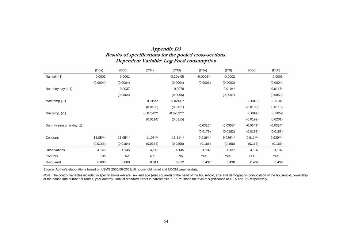
64

Appendix D3 Results of specifications for the pooled cross-sections.

Dependent Variable: Log Food consumption

(D3a) (D3b) (D3c) (D3d) (D3e) (D3f) (D3g) (D3h)

Rainfall (-1) 0.0002 0.0001

-3.20e-05 -0.0006** -0.0002

-0.0003

(0.0004) (0.0004) (0.0004) (0.0003) (0.0003) (0.0004)

No. rainy days (-1) 0.0037

0.0078

-0.0104*

-0.0117*

(0.0064)

(0.0066)

(0.0057)

(0.0059)

Max temp (-1)

0.0195* 0.0241**

-0.0018 -0.0101

(0.0106) (0.0111)

(0.0109) (0.0115)

Min temp. (-1)

-0.0754*** -0.0763***

-0.0088 -0.0059

(0.0114) (0.0115)

(0.0199) (0.0201)

Dummy season (rainy=1)

-0.0316* -0.0355* -0.0349* -0.0324*

(0.0179) (0.0182) (0.0185) (0.0187)

Constant 11.05*** 11.05*** 11.05*** 11.11*** 9.916*** 9.926*** 9.911*** 9.929***

(0.0163) (0.0164) (0.0164) (0.0206) (0.166) (0.166) (0.166) (0.166)

Observations 4,145 4,145 4,145 4,145 4,137 4,137 4,137 4,137

Controls No No No No Yes Yes Yes Yes

R-squared 0.000 0.000 0.011 0.012 0.437 0.438 0.437 0.438

Source: Author’s elaborations based on LSMS 2005/06-2009/10 household panel and UDOM weather data.

Note: The control variables included in specifications e-h are: sex and age (also squared) of the head of the household, size and demographic composition of the household, ownership of the house and number of rooms, year dummy. Robust standard errors in parenthesis. *, **, *** stand for level of significance at 10, 5 and 1% respectively.

65

Appendix E Complete results of specifications (1)-(16).

Dependent Variable: Log Food consumption (monthly, adj.)

Table 20 Econometric results (complete), fixed effect estimation.

(1) (2) (3) (4) (5) (6)

Sex head HH (F=1) -0.0718 -0.131** -0.0721 -0.130** -0.0754 -0.138**

(0.0497) (0.0657) (0.0494) (0.0654) (0.0498) (0.0657)

Age head HH 0.0133 0.0213* 0.0139* 0.0216* 0.0134* 0.0211*

(0.00811) (0.0117) (0.00812) (0.0117) (0.00807) (0.0117)

Age head squared -0.000108 -0.000190 -0.000114 -0.000192 -0.000110 -0.000193

(8.01e-05) (0.000123) (8.02e-05) (0.000123) (7.96e-05) (0.000123)

HH size 0.0667*** 0.0602*** 0.0668*** 0.0599*** 0.0660*** 0.0601***

(0.00705) (0.00864) (0.00705) (0.00862) (0.00709) (0.00869)

Share males 0-5 0.529* 1.446*** 0.539** 1.464*** 0.558** 1.506***

(0.273) (0.468) (0.272) (0.470) (0.274) (0.471)

Share males 6-11 0.854*** 1.841*** 0.860*** 1.854*** 0.878*** 1.895***

(0.282) (0.475) (0.281) (0.478) (0.283) (0.478)

Share males 12-17 0.678** 1.615*** 0.683** 1.625*** 0.693** 1.654***

(0.274) (0.483) (0.273) (0.486) (0.275) (0.486)

Share males 18-64 0.570** 1.466*** 0.574** 1.476*** 0.578** 1.502***

(0.255) (0.454) (0.255) (0.457) (0.256) (0.459)

Share males >65 0.0527 0.683 0.0732 0.701 0.0630 0.714

(0.345) (0.564) (0.343) (0.565) (0.346) (0.569)

Share females 0-5 0.755*** 1.636*** 0.763*** 1.649*** 0.773*** 1.687***

(0.276) (0.476) (0.275) (0.478) (0.276) (0.479)

Share females 6-11 0.868*** 1.763*** 0.865*** 1.767*** 0.887*** 1.814***

(0.265) (0.468) (0.265) (0.472) (0.266) (0.472)

Share females 12-17 0.721*** 1.790*** 0.720*** 1.794*** 0.725*** 1.795***

(0.263) (0.463) (0.263) (0.466) (0.264) (0.467)

Share females 18-64 0.492** 1.419*** 0.501** 1.434*** 0.502** 1.434***

(0.246) (0.441) (0.246) (0.444) (0.247) (0.446)

Own House 0.131** 0.113 0.132** 0.111 0.129** 0.105

(0.0576) (0.0737) (0.0576) (0.0741) (0.0581) (0.0752)

No. Rooms 0.0487*** 0.0396*** 0.0479*** 0.0395*** 0.0489*** 0.0396***

(0.00893) (0.00981) (0.00896) (0.00981) (0.00887) (0.00974)

Owned Parcels (No.)

0.0418***

0.0421***

0.0416***

(0.0127)

(0.0126)

(0.0128)

Owned Parcels Size 6.81e-06

4.14e-05

0.000146

(0.000521)

(0.000514)

(0.000516)

Continued…

66

Continued (1) (2) (3) (4) (5) (6)

Education HH (2)

0.0654

0.0702

0.0448

(0.179)

(0.179)

(0.184)

Education HH (3)

0.192

0.193

0.161

(0.200)

(0.200)

(0.205)

Education HH (4)

0.0824

0.0846

0.0730

(0.208)

(0.209)

(0.213)

Education HH (5)

0.0836

0.0843

0.0743

(0.187)

(0.187)

(0.192)

Education HH (6)

0.172

0.171

0.142

(0.204)

(0.204)

(0.208)

Education HH (7)

0.336

0.336

0.287

(0.254)

(0.252)

(0.254)

Rainfall (-1) -0.000839** -0.00116*** -0.000386 -0.000826

(0.000340) (0.000394) (0.000415) (0.000503)

Rainy days (-1)

-0.0136* -0.00964

(0.00736) (0.00899)

Max temp. (-1)

0.00864 0.00478

(0.0141) (0.0170)

Min temp. (-1)

0.00296 -0.0277

(0.0202) (0.0227)

Dummy season (R=1) -0.0738*** -0.0685** -0.0795*** -0.0724*** -0.0818*** -0.0736**

(0.0235) (0.0278) (0.0237) (0.0278) (0.0248) (0.0287)

Dummy year (2009=1) 0.0274 0.0346 0.0292 0.0359 0.0271 0.0262

(0.0234) (0.0287) (0.0234) (0.0288) (0.0240) (0.0295)

Constant 9.497*** 8.390*** 9.483*** 8.368*** 9.481*** 8.418***

(0.291) (0.530) (0.291) (0.533) (0.290) (0.539)

Observations 4,137 2,937 4,137 2,937 4,137 2,937

R-squared 0.137 0.166 0.139 0.167 0.135 0.162

Number of HH 2,213 1,694 2,213 1,694 2,213 1,694

Source: Author’s elaborations based on LSMS 2005/06-2009/10 household panel and UDOM weather data.

Note:. Robust standard errors in parenthesis. *, **, *** stand for level of significance at 10, 5 and 1% respectively.

67

Table 21 Econometric results (complete), fixed effects estimations. Persistency checks.

Dep.var=ln food cons. (7) (8) (9) (10) (11) (12)

Sex head HH (F=1) -0.0726 -0.138** -0.0729 -0.136** -0.0772 -0.131**

(0.0497) (0.0660) (0.0493) (0.0653) (0.0498) (0.0658)

Age head HH 0.0135* 0.0215* 0.0143* 0.0221* 0.0130 0.0213*

(0.00808) (0.0116) (0.00810) (0.0116) (0.00810) (0.0116)

Age head squared -0.000109 -0.000191 -0.000116 -0.000195 -0.000105 -0.000198

(7.98e-05) (0.000122) (8.01e-05) (0.000122) (8.01e-05) (0.000123)

HH size 0.0673*** 0.0605*** 0.0675*** 0.0603*** 0.0664*** 0.0605***

(0.00704) (0.00862) (0.00706) (0.00860) (0.00710) (0.00867)

Share males 0-5 0.514* 1.425*** 0.523* 1.445*** 0.560** 1.518***

(0.272) (0.464) (0.272) (0.465) (0.276) (0.471)

Share males 6-11 0.854*** 1.839*** 0.861*** 1.857*** 0.878*** 1.899***

(0.282) (0.472) (0.282) (0.474) (0.284) (0.478)

Share males 12-17 0.681** 1.618*** 0.686** 1.633*** 0.698** 1.668***

(0.274) (0.480) (0.274) (0.481) (0.276) (0.486)

Share males 18-64 0.567** 1.455*** 0.571** 1.470*** 0.591** 1.539***

(0.255) (0.450) (0.255) (0.451) (0.257) (0.458)

Share males >65 0.0536 0.688 0.0710 0.693 0.0512 0.730

(0.343) (0.560) (0.342) (0.560) (0.346) (0.571)

Share females 0-5 0.746*** 1.622*** 0.753*** 1.638*** 0.796*** 1.714***

(0.275) (0.471) (0.275) (0.473) (0.278) (0.479)

Share females 6-11 0.866*** 1.758*** 0.862*** 1.761*** 0.896*** 1.839***

(0.264) (0.464) (0.265) (0.466) (0.267) (0.471)

Share females 12-17 0.723*** 1.796*** 0.722*** 1.804*** 0.725*** 1.801***

(0.262) (0.457) (0.263) (0.459) (0.265) (0.466)

Share females 18-64 0.492** 1.420*** 0.500** 1.436*** 0.502** 1.453***

(0.246) (0.437) (0.246) (0.439) (0.249) (0.446)

Own House (Yes=1) 0.132** 0.117 0.133** 0.116 0.124** 0.103

(0.0575) (0.0734) (0.0575) (0.0735) (0.0577) (0.0753)

No. Rooms 0.0482*** 0.0393*** 0.0474*** 0.0394*** 0.0486*** 0.0392***

(0.00892) (0.00978) (0.00892) (0.00973) (0.00891) (0.00970)

Owned parcels (No.)

0.0396***

0.0398***

0.0385***

(0.0127)

(0.0126)

(0.0127)

Owned Parcels Size 7.31e-06

5.57e-05

0.000119

(0.000523)

(0.000514)

(0.000539)

Head education (2)

0.0795

0.0787

0.0653

(0.174)

(0.174)

(0.182)

Head education (3)

0.202

0.199

0.192

(0.196)

(0.196)

(0.204)

Head education (4)

0.0964

0.0987

0.0815

(0.204)

(0.205)

(0.212)

Head education (5)

0.101

0.0983

0.0881

(0.182)

(0.182)

(0.191)

Continued…

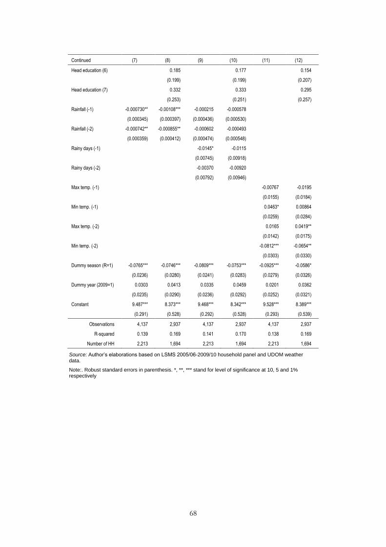
68

Continued (7) (8) (9) (10) (11) (12)

Head education (6)

0.185

0.177

0.154

(0.199)

(0.199)

(0.207)

Head education (7)

0.332

0.333

0.295

(0.253)

(0.251)

(0.257)

Rainfall (-1) -0.000730** -0.00108*** -0.000215 -0.000578

(0.000345) (0.000397) (0.000436) (0.000530)

Rainfall (-2) -0.000742** -0.000855** -0.000602 -0.000493

(0.000359) (0.000412) (0.000474) (0.000548)

Rainy days (-1)

-0.0145* -0.0115

(0.00745) (0.00918)

Rainy days (-2)

-0.00370 -0.00920

(0.00792) (0.00946)

Max temp. (-1)

-0.00767 -0.0195

(0.0155) (0.0184)

Min temp. (-1)

0.0463* 0.00864

(0.0259) (0.0284)

Max temp. (-2)

0.0165 0.0419**

(0.0142) (0.0175)

Min temp. (-2)

-0.0812*** -0.0654**

(0.0303) (0.0330)

Dummy season (R=1) -0.0765*** -0.0746*** -0.0809*** -0.0753*** -0.0925*** -0.0586*

(0.0236) (0.0280) (0.0241) (0.0283) (0.0279) (0.0326)

Dummy year (2009=1) 0.0303 0.0413 0.0335 0.0459 0.0201 0.0362

(0.0235) (0.0290) (0.0236) (0.0292) (0.0252) (0.0321)

Constant 9.487*** 8.373*** 9.468*** 8.342*** 9.528*** 8.389***

(0.291) (0.528) (0.292) (0.528) (0.293) (0.539)

Observations 4,137 2,937 4,137 2,937 4,137 2,937

R-squared 0.139 0.169 0.141 0.170 0.138 0.169

Number of HH 2,213 1,694 2,213 1,694 2,213 1,694

Source: Author’s elaborations based on LSMS 2005/06-2009/10 household panel and UDOM weather data.

Note:. Robust standard errors in parenthesis. *, **, *** stand for level of significance at 10, 5 and 1% respectively

69

Table 22 Econometric results (complete), fixed effect estimation. All weather deviations and

persistency.

Dep.var=ln food cons. (13) (14) (15) (16)

Sex head HH -0.0730 -0.131** -0.0754 -0.131**

(0.0495) (0.0658) (0.0496) (0.0659)

Age head HH 0.0138* 0.0211* 0.0136* 0.0214*

(0.00811) (0.0117) (0.00814) (0.0115)

Age head squared -0.000113 -0.000187 -0.000109 -0.000192

(8.01e-05) (0.000123) (8.05e-05) (0.000121)

HH size 0.0666*** 0.0604*** 0.0676*** 0.0610***

(0.00709) (0.00873) (0.00711) (0.00868)

Share males 0-5 0.540** 1.467*** 0.530* 1.459***

(0.273) (0.469) (0.275) (0.466)

Share males 6-11 0.860*** 1.855*** 0.863*** 1.860***

(0.282) (0.477) (0.285) (0.476)

Share males 12-17 0.683** 1.627*** 0.692** 1.643***

(0.274) (0.484) (0.276) (0.482)

Share males 18-64 0.573** 1.481*** 0.583** 1.505***

(0.255) (0.456) (0.257) (0.453)

Share males >65 0.0740 0.703 0.0626 0.721

(0.343) (0.563) (0.342) (0.563)

Share females 0-5 0.764*** 1.654*** 0.775*** 1.664***

(0.276) (0.477) (0.277) (0.474)

Share females 6-11 0.867*** 1.771*** 0.875*** 1.789***

(0.265) (0.470) (0.267) (0.467)

Share females 12-17 0.720*** 1.792*** 0.724*** 1.801***

(0.264) (0.464) (0.265) (0.459)

Share females 18-64 0.499** 1.429*** 0.499** 1.444***

(0.247) (0.443) (0.249) (0.442)

Own House 0.133** 0.105 0.129** 0.105

(0.0577) (0.0743) (0.0573) (0.0742)

No. Rooms 0.0482*** 0.0395*** 0.0477*** 0.0391***

(0.00894) (0.00983) (0.00894) (0.00973)

Owned parcels (No.)

0.0434*** 0.0393***

(0.0126)

(0.0125)

Owned Parcels Size 2.66e-05

1.06e-05

(0.000527) (0.000558)

Head education (2)

0.0674

0.0973

(0.179)

(0.172)

Head education (3)

0.186

0.219

(0.200)

(0.195)

Head education (4)

0.0771

0.0945

(0.208)

(0.203)

Head education (5)

0.0793

0.107

(0.187)

(0.180)

Continued…

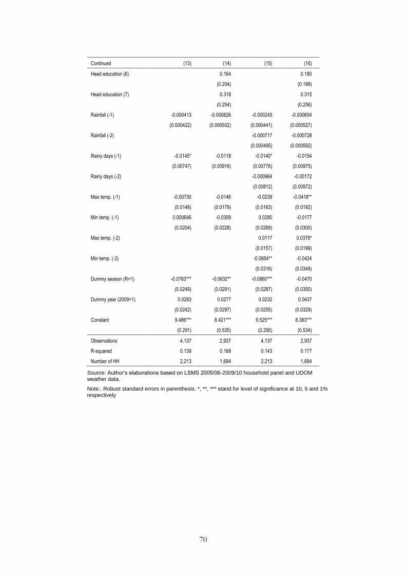
70

Continued (13) (14) (15) (16)

Head education (6)

0.164

0.180

(0.204)

(0.199)

Head education (7)

0.318

0.315

(0.254)

(0.256)

Rainfall (-1) -0.000413 -0.000826 -0.000245 -0.000604

(0.000422) (0.000502) (0.000441) (0.000527)

Rainfall (-2)

-0.000717 -0.000728

(0.000495) (0.000592)

Rainy days (-1) -0.0145* -0.0118 -0.0140* -0.0154

(0.00747) (0.00916) (0.00776) (0.00975)

Rainy days (-2)

-0.000964 -0.00172

(0.00812) (0.00972)

Max temp. (-1) -0.00730 -0.0146 -0.0239 -0.0418**

(0.0148) (0.0179) (0.0163) (0.0192)

Min temp. (-1) 0.000646 -0.0309 0.0280 -0.0177

(0.0204) (0.0228) (0.0269) (0.0300)

Max temp. (-2)

0.0117 0.0378*

(0.0157) (0.0199)

Min temp. (-2)

-0.0654** -0.0424

(0.0316) (0.0349)

Dummy season (R=1) -0.0763*** -0.0632** -0.0860*** -0.0470

(0.0249) (0.0291) (0.0287) (0.0350)

Dummy year (2009=1) 0.0283 0.0277 0.0232 0.0437

(0.0242) (0.0297) (0.0255) (0.0329)

Constant 9.486*** 8.421*** 9.525*** 8.383***

(0.291) (0.535) (0.295) (0.534)

Observations 4,137 2,937 4,137 2,937

R-squared 0.139 0.168 0.143 0.177

Number of HH 2,213 1,694 2,213 1,694

Source: Author’s elaborations based on LSMS 2005/06-2009/10 household panel and UDOM weather data.

Note:. Robust standard errors in parenthesis. *, **, *** stand for level of significance at 10, 5 and 1% respectively

71

Appendix F Effects of weather deviations in particular seasons

In the previous sections we emphasized the seasonal pattern of food consump-tion in Uganda. In order to further check for this, we investigate how much of the weather deviations impacts on food consumption depend on the season in which they occur. To do this we added to the specifications an interaction vari-able of whether the household was interviewed in the rainy season with the deviation variable we wanted to take care of. Here we consider the minimum and maximum temperatures. Table 23 shows the results, to discuss the sea-sonal pattern we compare the results of specifications (5)-(6) with (21)-(22) at first and (13)-(14) with (23)-(24) after.

When comparing (5)-(6) with (17)-(18) we immediately note that both magnitude and level of significance of the coefficients have changed with the introduction of the interaction variable, suggesting the importance of the sea-son when the shock occurs for the determination of food consumption. In fact, on average maximum and minimum temperatures seem to have a greater impact on food consumption (-3.56% with respect to 0.86% and -0.87% with respect to 0.30% for a one degree deviation in the maximum and minimum temperatures respectively). However, the coefficients are not significant. On the other side, the dummy for the rainy season as period of interview also ex-perienced an increase of magnitude, while the significance of both the dummy and the interaction variables range from 5% to 1% level. Ultimately, we have that if the household had been interviewed in the dry season, a one degree temperature deviation during the previous rainy season wouldn’t have affected food consumption. On the contrary, if the household had been interviewed during the rainy season, it would have experienced a decrease in consumption by 9.12% in the case of a one degree deviation in maximum temperatures and 10.55% in the case of a one degree deviation in minimum temperatures (a higher effect with respect to (5) and (6)). This can be understood with the fact that when the interview takes place in the rainy season, it means that we are analysing the impact of temperature deviations in the previous dry season. Hence, a warmer dry season constitute a potential damage for the harvest, in the end affecting food consumption in the current season while the same shock during a rainy season would have had smaller effects, probably a quicker maturation of the crops if the rainfall and number of rainy days remained fairly stable.

When we consider all the weather deviations together with their respective dummies for the season, we find that all the coefficients have increased of magnitude (the dummy for the rainy season has almost doubled). Moreover, the impact of a deviation in the maximum temperatures is now very important. In fact, for a household interviewed in the dry season, a one degree deviation in the maximum temperature in the previous rainy season from the long term mean, brings, other weather variables being stable, a decrease in the food con-sumption by 6.54% with a 1% level of significance. Eventually, this impact can be explained by the damages to the crops during their growing period due to the too hot weather. If the household was interviewed in the rainy season, in-stead, the negative effect would be higher and amounting on average to 14.74% food consumption less for one degree deviation in maximum tempera-tures during the previous dry season. Hence, we can argue that temperatures deviations have more negative impacts on food consumption if they occur dur-

72

ing a dry season than during a rainy season, we argue in close connection with the damages to the crop yields deriving from that warmer period.

Table 23 Econometric results. Temperatures, other deviations and seasonal pattern.

ln food consumption expenditures

Variable (21) (22) (23) (24)

Max temp. (-1) -0.0356 -0.0504 -0.0654*** -0.0881**

(0.0233) (0.0349) (0.0247) (0.0368)

Min temp. (-1) -0.0087 -0.0151 0.0023 0.0030

(0.0225) (0.0266) (0.0243) (0.0288)

Rainfall (-1) -0.00101 -0.00148*

(0.0006) (0.0009)

No. Rainy days (-1) -0.0230** -0.0259**

(0.0094) (0.0125)

Max temp (-1) X dummy rainy season 0.0578** 0.0665* 0.0762*** 0.0916**

(0.0234) (0.0358) (0.0250) (0.0372)

Min temp (-1) X dummy rainy season 0.0435* 0.0223 0.0358 0.00701

(0.0224) (0.0277) (0.0234) (0.0296)

Rainfall (-1) X dummy rainy season

0.0010 0.0011

(0.0008) (0.0011)

No. rainy days (-1) X dummy rainy season

0.0092 0.0165

(0.0147) (0.0195)

Dummy seas. (R=1) -0.149*** -0.115** -0.158*** -0.118**

(0.0337) (0.0476) (0.0371) (0.0548)

N 4,137 2,589 4,137 2,589

NH 2,213 1,547 2,213 1,547

R2 within 0.140 0.140 0.145 0.148

R2 between 0.384 0.355 0.375 0.351

R2 overall 0.330 0.317 0.324 0.316

F-test (p-value) for interac-tion terms

0.0028 0.1071 0.0076 0.1091

Source: Author’s elaborations based on LSMS 2005/06-2009/10 household panel and UDoM weather data.

Note: The control variables included in the odd numbered specifications are: sex and age (also squared) of the head of the household, size and demographic composition of the household, ownership of the house and number of rooms, year dummy. The even numbered specifications include also the education of the head of the household and size of the owned parcels of land. Robust standard errors in parenthesis. *, **, *** stand for level of significance at 10, 5 and 1% respectively.

Similar results are obtained when we control also for land ownership and education of the head of the household but generally the level of significance lowers or fades away, again suggesting for better insurance for those that have land assets even though this variable per se doesn’t have a significant impact..

73

Appendix G Effects of persistency in weather deviation and seasonal pattern

We look now at the effect of weather deviations considering also the per-sistency of effects from deviations occurred two seasons before the interview again making use of the instrumental variables method. Elaborating on the previous analysis we look to temperature deviations and to all the weather deviations together. Table 24 shows the results: specifications (25) and (27) control for household demographic composition, sex and age of the head, house ownership and number of rooms in the house while (26) and (27) con-trol also for size of land owned and education of the head. The F-test for the joint significance of the interaction terms is significant at conventional levels for (25) and (27) but not for (26) and (28). Hence, further investigations should be done on the effects of shocks and land ownership/head education.

When analysing (25), we have that, on average, when the household is in-terviewed in the dry season and experienced a deviation in minimum tempera-tures in the previous rainy season, it didn’t have a significant impact on food consumption. In the case it experienced a one degree deviation in maximum temperatures, instead, on average its consumption would decrease by 5.66% with a 5% level of significance. When the deviations were experienced two sea-sons before (during a dry/harvesting season) the household would have ex-perienced positive effects on current consumption in the case of a one degree deviation in maximum temperatures but non-significant negative effects for the same variation in minimum temperatures. It seems that maximum temperature deviations have persistent effects on food consumption but their impact is now positive. These results are not in line with our expectations form the pre-vious analysis.

On the other side, when the household was interviewed in a rainy season, the reported deviations were referred to the previous dry (-1) and rainy (-2) season. In light of the joint significance of minimum temperatures when tested with their respective interaction variables, on average we can say that a one de-gree deviation in period (-1) would cause a decrease in food consumption of 8.8% (bigger compared to the specification without interactions) while the same deviation in period (-2) would cause a decrease of 21.89% (as compared to about -8%). Similar results can be computed for the deviations in maximum temperatures and for other weather deviations in the other specifications.

To conclude, we can then argue that, if at a first sight temperature devia-tions didn’t seem to affect food consumption or seemed more damaging if oc-curring in the dry season, explicitly accounting for the season when the devia-tion took place gives us more insights on the importance of minimum temperature deviations in the rainy seasons in determining the availability of food (being the agriculture activity of subsistence) and the food consumption.

74

Table 24 Econometric results. Effects of consecutive weather deviations and seasonal pattern.

ln food consumption expenditures

Variable (25) (26) (27) (28)

Rainfall (-1) -0.0007 -0.0008

(0.0007) (0.0010)

No. Rainy days (-1) -0.0253*** -0.0289**

(0.0096) (0.0132)

Max temp. (-1) -0.0566** -0.0780** -0.0803*** -0.107***

(0.0246) (0.0352) (0.0270) (0.0373)

Min temp. (-1) 0.0194 -0.0144 0.0123 -0.0379

(0.0398) (0.0497) (0.0426) (0.0552)

Rainfall (-1) X dummy rainy season 0.0009 0.0006

(0.0009) (0.0012)

No. rainy days (-1) X dummy rainy sea-son

0.0100 0.0142

(0.0157) (0.0209)

Max temp (-1) X dummy rainy season 0.0665** 0.0635 0.0775** 0.0789*

(0.0283) (0.0408) (0.0312) (0.0430)

Min temp (-1) X dummy rainy season 0.0570 0.103 0.0530 0.0942

(0.0525) (0.0701) (0.0562) (0.0773)

Rainfall (-2) -0.0003 -0.0009

(0.0008) (0.0010)

No. Rainy days (-2) -0.0119 -0.0132

(0.0127) (0.0168)

Max temp. (-2) 0.0277* 0.0507** 0.0155 0.0279

(0.0163) (0.0229) (0.0191) (0.0259)

Min temp. (-2) -0.0585 -0.0322 -0.0332 2.42e-05

(0.0449) (0.0573) (0.0470) (0.0624)

Rainfall (-2) X dummy rainy season -0.0004 0.0006

(0.0010) (0.0013)

No. rainy days (-2) X dummy rainy sea-son

0.0191 0.0258

(0.0159) (0.0224)

Max temp (-2) X dummy rainy season -0.0138 0.00297 0.0023 0.0290

(0.0295) (0.0378) (0.0318) (0.0411)

Min temp (-2) X dummy rainy season -0.0144 -0.0758 -0.0175 -0.0858

(0.0525) (0.0664) (0.0561) (0.0747)

Dummy season (rainy=1) -0.146*** -0.0964* -0.156*** -0.102*

(0.0365) (0.0512) (0.0400) (0.0614)

N 4,137 2,589 4,137 2,589

NH 2,213 1,547 2,213 1,547

R2 within 0.144 0.149 0.139 0.140

Source: Author’s elaborations based on LSMS 2005/06-2009/10 household panel and UDoM weather data.

Note: The control variables included in the odd numbered specifications are: sex and age (also squared) of the head of the household, size and demographic composition of the household, ownership of the house and number of rooms, year dummy. The even numbered specifications include also the education of the head of the household and size of the owned parcels of land. Robust standard errors in parenthesis. *, **, *** stand for level of significance at 10, 5 and 1% respectively.

75

Appendix H Map of Uganda with synoptic stations

Map 1 Map of Uganda (regions and districts) with the 13 synoptic stations.

Source: Adapted from http://commons.wikimedia.org/wiki/File:UgandaRegionsLegend.png, accessed 13

November 2012