weather effects on electricity loads modeling and forecasting

Final Report EPA Weather Effects on Electricity Loads of 48

Weather Effects on Electricity Loads: Modeling and Forecasting 12 December 2005

Christian Crowley and Frederick L. Joutz

Research Program on Forecasting Department of Economics

The George Washington University

Prepared for USEPA

Summary of Findings We investigated climate change-driven effects on electricity demand. The research focused on the estimating the impact of higher temperatures on electricity consumption using hourly data and annual data. The Pennsylvania-New Jersey-Maryland (PJM) Independent System Operating (ISO) or mid-Atlantic council region of the North American Electric Reliability council was primary area for the study. Additional data was used from the East Central Area Reliability (ECAR) and Southeastern Electric Reliability council (SERC). Scenarios were constructed to present the impact of a 2 degree Fahrenheit increase in temperatures. Short-run and long-run models were used in generating the scenarios. The short-run models were constructed to estimate the sensitivity of the daily load curve to hourly temperature for all ten load regions in the PJM separately. The responses are conditional on a given stock of electricity using equipment, building shell efficiencies, stock of electricity generation facilities, and transmission network. Simulations were run to examine the effect of the temperature increase. These short-run models are especially useful for their detail and relating peak loads and changes in the load curve or human response in terms of electricity demand. The long-run model results are based on a “general equilibrium approach” for the entire U.S. The National Energy Modeling System (NEMS) which the Energy Information Administration (EIA) uses in making projections to 2025-2030 was the primary model. In the NEMS, households and firms can adjust stock of electricity using equipment and building shell efficiencies in response to relative prices, economic activity, and technology choices. Similarly, the electric utility sector adjust the mix and stock of generating facilities and transmission network in response to expected demand, relative prices of input sources, technology, and regulatory environment. The output from the short-run and long-run consumption models in terms of load projections and elasticities serve as the inputs to supply side models which allocate or dispatch the electricity from the generation stock and mix to meet the load. Given the dispatch assumptions, that model will project with electricity sector emissions, with a focus on NOx. Climate change will alter the level and timing of electricity demands, as well as the thermal efficiency of electricity generating units. With a given capital stock of generating plant (short run analysis), this will change their operations and emissions. Even in the presence of seasonal or annual emissions caps, emissions might then increase during the warmest days when ozone episodes are most likely to occur. In the long run, the mix and amounts of various types of generation technologies will adjust, and if climate change occurs, the resulting generation plant will be different than if climate change does not occur. This has further implications for the


timing and amount of emissions. This portion of the research project developed and demonstrated methods for obtaining temporal and spatial distributions of NOx emissions from power plants, and for quantifying the effects of climate change scenarios on those distributions. In Section 1 of this report we explain the methodology and models used in the short-run (hourly) responses of electricity consumption to changes in temperature. Section 2, contains results on the potential long-run impacts of temperature on electricity loads. Two different modeling approaches were used. The first is based on the U.S. Energy Information Administration’s National Energy Modeling System (NEMS) and the second is based on a regional econometric model by sector of electricity consumption. In the next section, we provide a brief background on the analyses of weather effects on electricity consumption. In Section 4, the database programs used in the analysis are briefly described so that the work may be replicated. The final section provides other explicit accomplishments of this research projects. All material is provided in electronic format on a CD by section.

The major findings concerning the short- and long-run effects of climate change on electricity loads are summarized as follows:

1. Short-run Effects of Weather on Electricity Loads

Hourly forecasting models were built and parameterized using approximately eight years’ worth of hourly temperature and load data for the ten utility companies of the PJM control area. Two seasonal OLS models were developed (Summer and Winter) using deterministic variables (Day, Month, Holiday), linear, quadratic, and cubic functions of hourly temperature ( 32 ,, TTT ) and an autoregressive component (1-hour, 2-hour, 3-hour, and 24-hour lagged loads). The results of testing over fifty model specifications for goodness of fit indicate that a model including the variables listed above, and with a single parameter for each temperature variable, is the specification with the best explanatory power for the utilities in the PJM region.

A simulation of a 2°F increase in temperature for July and August 2000 resulted in a 4.6% increase in electricity demand for the region as a whole. These being the peak cooling demand months, the average increase over the year would likely be somewhat lower. These results are similar in magnitude to resultsreported for a simulation of electricity demand in California by Baxter and Calandri (1992), who found a 3.8% increase over the year for a similar warming scenario.

As a verification of the OLS results, a set of hourly models was also developed using the artificial neural network (ANN) approach. ANN modeling for the Baltimore region within PJM showed that simulated electricity demand using ANNs is similar to simulated demand using OLS models, in terms of magnitude and variation of hourly loads above the baseline forecast (the forecast made in the absence of any temperature change). Over a simulation period from July 1, 2000 through August 30, 2000, for a uniform two-degree Fahrenheit increase in temperature, the ANN specification predicted an average increase of 4.5 percent over the baseline forecast, with individual hourly models’ results ranging from 2.0 percent up to 6.9 percent above the baseline ANN forecast. The OLS specification for Baltimore only (as opposed to all of PJM), meanwhile predicted a 4.4 percent increase above baseline, with individual hourly models’ results ranging from 2.1 percent up to 6.3 percent above the baseline OLS forecast. 2. Long-run Effects of Weather on Electricity Loads


The NEMS attempts to capture the interaction between the energy markets and economic activity. In the NEMS, households and firms can adjust the stock of electricity using equipment and building shell efficiencies in response to relative prices, economic activity, and technology choices. Similarly, the electric utility sector adjusts the mix and stock of generating facilities and transmission network in response to expected demand, relative prices of input sources, technology, and the regulatory environment. Economic growth and demographic trends are included in making the projections by the 9 U.S. Census regions. Weather and temperature are important drivers for electricity consumption. More than 40% of end-use energy consumption is related to the heating and cooling needs in the residential and commercial sectors. Electricity consumption forecasting models typically use thresholds for defining when the cooling and heating needs are required. A fairly standard set of thresholds are temperatures above 72 degrees Fahrenheit and below 65 degrees Fahrenheit respectively. The difference in the daily high and the 72 degrees is referred to as a cooling-degree day (CDD); a similar calculation is performed to construct a heating-degree day (HDD) by taking the difference between the low and 65 degrees. We constructed a scenario based on the average of the 5 warmest summers and the 5 warmest winters relative to the remaining periods to examine the effects of a warming in temperature. This yields approximately a 2.09 degree Fahrenheit increase in CDDs and almost 4 degree Fahrenheit decrease in HDDs. These temperatures are consistent with climate change considered by the ICCG. Our hypothesis was that warmer weather would change the annual pattern or shape of the load from winter to summer. In addition, the implied daily load could change more toward peaking periods. Higher temperatures would reduce residential and commercial demand for space heating in the winter and increase the demand for space cooling in the summer. The former is typically supplied by fossil fuels while the later is almost exclusively provided by electricity. The impact could lead to greater relative peaking capacity needs. The electricity demand modules of NEMS, particularly residential and commercial, calculate electric loads based conditional on the CDD and HDD variables along with the economic and embodied technical change in the stock of energy using equipment and structures. The load is allocated on what is called the “load curve”which illustrates the relationship of power consumption/supply during sub-periods of the period covered. This can be broken out be season, day of the week, and time of day.

The impact of temperature warming in the summer scenario had two important effects. First, average load demand was about 2.7 percent higher in the summer months. Second, peak demand was 5.4 percent higher. Thus, the results suggest an important impact on the load shape. Climate change will have a disproportionate effect on load in the peak periods. This may be exactly the periods when ozone is likely to be more of a problem. The JHU teams’ dispatch and supply emissions models and weather models will examine these potential these effects.

3. Additional Accomplishments

• The EPA STAR grant support a research assistant, Christian Crowley, to formulate and complete his PhD dissertation, on economic modeling as applied to natural resource issues. Portions from two his three essays are presented in this report. Christian Crowley defended his dissertation on Monday, December 12, 2005. The two essays are included in the report: 1) Electricity Demand Forecasting and


Climate Change: Results for the PJM Region and 2) Forecasting Electricity Demand: A Neural Network Approach.

• The grant supported presentations national and international conferences on energy demand In addition, several working papers are in process and will be submitted for publication in professional journals. They include:

o RER/Itron MetrixND Users Meeting (September 2002), San Diego, CA o IAEE (July 2003), Mexico City o IAEE (July 2004), Washington, DC o INFORMS (October 2004), Denver, CO o IAEE (June 2005), Taipei o Working Paper: Seasonality and Weather Effects on Electricity Loads: Modeling and

Forecasting • The results from the consumption forecasting and simulation models were linked to supply and weather

models. The scenarios of hourly load projections and the long-run load projections for the PJM region estimated from this research were able to be fed into the supply side models for generating the dispatch of electricity and resulting emissions. In addition, simulations were performed based on weather models projections for hourly temperature warming scenario data for 1991-1997 and 2050-2055


Section 1: Background on Electricity Demand Modeling and Weather Section 1.1 Short-run or Hourly Models Bunn and Farmer (1985) and EPRI (1977) contain collections of papers on the modeling forecasting of hourly electricity loads. Total system loads were modeled by Schneider et al. (1985) in terms of base load, weather sensitive load, error adjustment, and a bias correction. Ackerman (1985) compared alternative forms of ARIMA models. Gupta (1985) proposed a model with seasonal time varying parameters to historical loads and weather information. The parameters were adaptive and would change in response to changing load processes. Ramanathan et al. (1997) developed a series of models for forecasting loads as functions of hourly, daily and seasonal factors, autoregressive components, and weather effects. The innovation of their framework was that rather than modeling the entire load series, they developed individual models for each hour. This proved productive in terms of explaining the data and in forecasting. In general, aggregate analyses have found that commercial and residential uses are much more sensitive to temperature increases than industrial uses, justifying the focus of this proposal on the former. These studies have usually concluded that climate warming would produce a few percentage point increase in cooling requirements, and a similar decrease in heating requirements (Scott et al., 1994; Morris et al., 1996; Sailor and Munoz, 1997); the canceling of the two effects often implies that the net impact on annual energy use may be relatively small (e.g., Darmstadter, 1993). As an example of such a study, Baxter and Calandri (1992) projected that a 1.9oC warming would increase California’s annual electricity requirements by 2.6%. What is more relevant, however, is how that change is distributed within the year. In particular, the greatest increases are likely to occur during weekdays during the air conditioning season, precisely at those times that tropospheric ozone violations occur. For instance, Baxter and Calandri’s (1992) analysis indicates that their assumed 1.9oC increase would magnify peak summer electricity demands by 3.7%. It is possible that the proportional increase during periods of high ozone may be even higher; however, no studies have analyzed climate’s effect on energy demands on a temporal scale fine enough to consider this possibility. One of this project’s purposes is to fill that gap. The result of using load duration curves in a long-run production simulation model is a set of estimates of average cost and emissions by generating unit type for a given period of time. This will permit a general assessment of the strength of the linkage between regional climate change and emissions of criteria pollutants. However, because of the high correlation between time-varying electricity demands (and thus emissions) and the meteorological conditions that influence ambient pollutant concentrations, the impact of that linkage upon concentrations and ensuing health effects must be based upon a detailed chronological simulation of both power system operations and pollutant transport and transformation. Utility experience across the U.S. shows that variations in weekday demands are most strongly associated with temperature, although wind, humidity, and cloud cover are also factors that are frequently considered in short-term models in Liu et al. (1996). Typically, 80% or more of the variation is associated with weather, and for systems we have studied, peak electric demands in the summer can easily vary by 25% or more because of day-to-day changes in temperature [Hobbs et al., 1998]. Section 1.2 Long-run Models


In Climate Change Impacts in the United States (NAST 2000) the National Assessment Synthesis Team identified areas where human and economic behavior would be affected by climate change. These effects may increase energy costs for consumers and firms, depending on the types of energy used and the geographic region considered. These impacts, and resulting feedback responses, may further impact cost effects and overall carbon emissions. One area the Team identified was heating and cooling requirements for residential and commercial buildings.

Rosenthal, Gruenspecht, and Moran (1995) worked with data from national building surveys and five global climate change models to estimate the cost impacts. They used historical regional weather data and expectations of future weather patterns, converting these into cooling and heating measures. Data on building and equipment stocks were converted into efficiency or intensity units to analyze the requirements for energy use and the resulting economic costs. The results of this study suggested that total U.S. energy requirementswould show a slight decrease in the aggregate in response to climate warming.

Hadley, Erickson, and Hernandez (2004) examined the impacts of climate warming using the National Energy Modeling System (NEMS) and a general circulation model of the Earth’s climate. The authorsconsidered two cases: a 2.1°F increase and a 6.0°F increase. They present results by U.S. Census region and find offsetting effects: heating needs decline in the winter while cooling needs increase in summer. Total energy consumption declines with the former effect, and increase with the latter. Responses vary by region as well as with the energy fuel mix considered and with end-use demand. On the whole, costs tend to decline in northern parts of the country, and tend to rise in the southern regions. Section 2: Short-run Modeling and Forecasting of Electricity

Section 2.1: OLS The General Model

A seasonal model was chosen to isolate differences between summer demand and winter demand. Hourly temperature terms include the level, the square and the cube of the temperature, to account for non-linearities in the temperature-load relationship. An autoregressive component accounts for the loads of previous hours. Deterministic variables capture the effects of different load patterns for different days of the week or holidays, and for the individual months within a model’s season. The summer months are June, July, August and September, while the winter months are December, January, February and March. The most general form of the summer model contains the full complement of variables:

7 3

01 1

4 4 42 3

1 1 1

log( )

( )

ht i iht i ihti i

i iht iht i iht iht i iht ihti i i

ht ht

Load Day Month

Month T Month T Month T

L Load e

β β δ

α γ λ

φ

= =

= = =

= + +

+ ⋅ + ⋅ + ⋅

+ ⋅ +

� �

� � � (1)

In Equation (1), the subscript ht refers to hour h on day t, T is the temperature, and Day and Month are dummies that take on the value of 1 or 0 to isolate the effects of the various weekdays (or holidays) and months. For any given model specification, there is a family of twenty-four related hourly models, one each for

1 24h = �


In the summer version of the model, �0 captures the combined effect of Monday and June. The next seven � terms capture Tuesday through Sunday and the Holiday variable, which takes on a value of 1 for days that fall on common holidays, and 0 otherwise. The three � terms represent July, August and September. The levels, squares and cubes of hourly temperature interact with the Month variables through the multipliers iα , iγand iλ , where i = 1, 2, 3, or 4, to represent June, July, August or September. As an example, the static

component of the electric load for hour h on Fridays ( )5β in July ( )1δ is given by the expression 2 3

0 5 1 2 2 2h h hT T Tβ β δ α γ λ+ + + + + .

The dynamic component of demand is given by the autoregressive portion of the model, 1 2 3 24

1 2 3 4( )L L L L Lφ φ φ φ φ= + + + , where L is the lag operator. This term captures the loads of the previous three

hours, as well as the previous day’s load. The winter model is similar in form to the summer model, referencing the winter months December, January, February and March. For the winter model, the constant term �0 captures the effects of Mondays and January. The goal of the modeling procedure is to investigate hourly demand elasticities with respect to temperature. Given the model specification in Equation (1), the elasticity for hour h in month j is given by

( )22 3hj hj hjhj hj hj hjT T Tη α γ λ= + + ⋅ , (2)

where hjT indicates the monthly mean temperature (in month j) for the hour under consideration (hour h).

Model Selection Carrying out the “general to specific” modeling approach advocated by Hendry (1993) involves

beginning with the general model listed above in Equation (1), then excluding classes of variables to generate a family of related, simplified models. To find a parsimonious model specification with the most explanatory power, Diebold (2001) recommends comparing the Akaike information criterion (AIC) and Schwartz information criterion (SIC) of the various models with the original, “unrestricted” model of Equation (1). The AIC and SIC are expressions of mean squared error, with a penalty for degrees of freedom1; these measures are commonly used for selecting among various forecasting models.

Ranking Models by Explanatory Power

Model statistics were calculated using EViews 4.1 (Quantitative Micro Software, 2002), for a group of fifty- three related candidate model specifications. Specification #1 is the unrestricted specification given in Equation 1. The remaining fifty-two model specifications were derived from a list of alternate hypotheses about the relationships among the variables in the unrestricted specification. These hypotheses take the form of restrictions to the parameters in Equation (1). A complete list of the models tested, and their generating hypotheses, is given in Appendix 1 for the summer model specifications, and Appendix 2 for the winter model specifications.

A mean AIC for Specification #1 was found by averaging the AIC scores across the family of twenty-four hourly models that use Specification #1 ( 1,tLoad =� up to 24,tLoad =�). A mean SIC score for

Specification #1 was derived similarly. In addition to the mean scores, a pair of median scores was calculated using the median AIC or SIC from the family of twenty-four hourly models. Similar composite scores were

1 ��=

−

=

==T

tt

TkT

tt eTSICe

T

TkAIC

1

21/

1

2 ;)/2exp(


found for all fifty-three candidate model specifications. The candidate specifications were then ranked by each of these “composite” selection criteria, from lowest to highest2 to consider which specifications created the best fitting models in the most parsimonious way. This model generation and ranking procedure was performed for each of the ten utility control regions within PJM3, once for the summer models, and once for the winter models.

Each selection criterion in turn, is examined in an attempt at identifying one “universal” model specification that performs well across the entire PJM area. Considering the top specifications across the utility regions, the summer models have a more clear-cut set of “winners” than the winter models do. Among the “composite” selection criteria, the mean-composites produced more consistent results than the median scores, giving stronger recommendations for the preferred models across all utility regions. Compared with the mean AIC, the mean SIC score tends to favor a smaller set of models across all regions, due to the SIC’s higher penalty for degrees of freedom. In light of these results, the mean-composite-SIC was chosen as the selection criterion for this study, as the most selective of the four criteria considered. Using the mean SIC score to choose the best model for each region resulted in two different specifications coming out ahead: for nine regions Specification #52 was the best, and for one region #49 had the lowest mean SIC.

The Winning Specification

The results of the selection process indicate that the explanatory power of a model is increased by

including the deterministic effects of weekdays, weekends, holidays and the months. Temperatures in level, squared and cubed terms also tend to add to the explanatory power of a model. The clear winner across all regions is model #52, which achieved the lowest mean SIC in nine of the ten PJM utility regions for both summer and winter, coming in second-lowest in the tenth region (BGE).

The specification for model #52 includes the full complement of deterministic variables (Day, Month, Holiday), the autoregressive components (1-hour, 2-hour and 3-hour lags, plus a 1-day lag), and one parameter each for the level, square and cube of the temperature. The assumption underlying Model #52 is that there is no variation in temperature effects across the months of the season, i.e. 4321 αααα === , and likewise for iγ and

iλ . In other words, the demand effect of the temperature level ( iα ) is the same in June as it is in July, August

or September, and likewise for the square (iγ ) and cube ( iλ ) of the temperature. These restrictions hold for

both summer and winter models (though the winter months are December, January, February and March). The parameterization of Specification #52 for the Hour 8 model of the AE region (Atlantic Electric Co.) is reported in Table 2.1.

The parameterization of Specification #52 for the Hour 8 model indicates small but highly significant negative Day effects (Tuesday through Sunday, and Holiday). The same is true for the Month effects, although July appears to be insignificantly different from zero. The Temperature effects are highly significant: small and negative for the temperature level; smaller still and positive for the square of temperature; minute and negative for the cube of temperature. Among the lagged loads, the load from the previous hour (listed as “Load_07(0)” in Table 2.1) and the load from the same hour on the previous day (“Load_08(–1)” in the table) are highly significant and have a positive effect on the load for Hour 8. The high R2 value reported for this model is typical for highly autocorrelated series that include lags in the model specification. This autocorrelation also accounts for the large and significant coefficient on the 1-hour lag.

2 Both AIC and SIC are measures of model error, thus a low score indicates a better model fit. 3 Error! Reference source not found. contains information on the utility companies in the PJM control area.


Dependent Variable: LOG(LOAD_08) Method: Least Squares Date: 04/28/04 Time: 14:45 Sample: 6/01/1995 9/30/1995 6/01/1996 9/30/1996 6/01/1997 9/30/1997 6/01/1998 9/30/1998 6/01/1999 9/30/1999 6/01/2000 9/30/2000 6/01/2001 9/30/2001 6/01/2002 9/30/2002 6/01/2003 9/30/2003 Included observations: 1098 Newey-West HAC Standard Errors & Covariance (lag truncation=6)

Variable Coefficient Std. Error t-Statistic Prob.

C 1.525062 0.184488 8.266477 0.0000 TUESDAY -0.004523 0.001528 -2.960444 0.0031 WEDNESDAY -0.004593 0.001531 -2.999382 0.0028 THURSDAY -0.004750 0.001341 -3.542811 0.0004 FRIDAY -0.003617 0.001483 -2.438794 0.0149 SATURDAY -0.026965 0.002636 -10.22842 0.0000 SUNDAY -0.039265 0.003404 -11.53554 0.0000 HOLIDAY -0.024218 0.005282 -4.584677 0.0000 JUL -0.001572 0.001467 -1.071752 0.2841 AUG -0.010664 0.001755 -6.076508 0.0000 SEP -0.027428 0.001585 -17.30021 0.0000 (JUN+JUL+AUG+SEP)*TEMP_08 -0.030828 0.008163 -3.776449 0.0002 (JUN+JUL+AUG+SEP)*TEMP_08^2 0.000410 0.000119 3.448763 0.0006 (JUN+JUL+AUG+SEP)*TEMP_08^3 -1.64E-06 5.72E-07 -2.867345 0.0042 LOG(LOAD_07(0)) 1.011322 0.038935 25.97456 0.0000 LOG(LOAD_06(0)) -0.186012 0.119803 -1.552649 0.1208 LOG(LOAD_05(0)) 0.054116 0.095028 0.569470 0.5692 LOG(LOAD_08(-1)) 0.017087 0.006160 2.773783 0.0056

R-squared 0.993694 Mean dependent var 7.065505 Adjusted R-squared 0.993595 S.D. dependent var 0.144466 S.E. of regression 0.011562 Akaike info criterion -6.065925 Sum squared resid 0.144375 Schwarz criterion -5.983937 Log likelihood 3348.193 F-statistic 10010.95 Durbin-Watson stat 1.773299 Prob(F-statistic) 0.000000

Table 2.1. Statistics for Specification #52, Hour 8 Model (AE region)

Elasticities for Specification #52

Figure 2.1 shows an average load curve for the AE region by hour. In the figure, the load reported for each hour is the average load at that hour over the month of July 2000. The load is measured in megawatt-hours (MWh) on the right-hand vertical axis. The left-hand vertical axis records the corresponding hourly temperature elasticities, shown as bars, and calculated using Equation (2). Shading of the hourly elasticity bars indicates significance: solid bars have temperature elasticities that are significant at 95%. Note that the elasticity depends on three estimated coefficients associated with the temperature: α , γ and λ , for the level, square and cube of the temperature. The solid (significant) bars in Figure 2.1 indicate significant values for all three coefficients (α , γ , λ ), elasticities with at least one insignificant coefficient are shown with hashed bars. Throughout this study, Hour 1 refers to the hour between midnight and 1:00 a.m.

Temperature elasticities appear to be lowest in the nighttime and early morning, with elasticities from 0.02 to 0.05 between the hours of 1 a.m. and 7 a.m. Though there is some air conditioning responsiveness on


hot nights, most consumers are asleep or otherwise “off- line” during these hours. With the start of the work day, temperature elasticity increases dramatically, rising above 0.19 between 7 a.m. and 10 a.m.: temperatures and loads rise as businesses open and people begin their daily activities. Throughout the working day, elasticities are more moderate, remaining between 0.08 and 0.12 from 10 a.m. to 4 p.m. Elasticities are relatively low during the late afternoon and into the night, falling to between 0.05 and 0.10 after 4 p.m., until the cycle repeats.

Temperature Elasticity and Load - AE July 2000

0.00

0.05

0.10

0.15

0.20

0.25

1 6 11 16 21

Hour of the Day

Ela

stic

ity

900

1200

1500

1800M

Wh

Temp Elasticity Load

(solid bars have significant t-stat)

Figure 2.1. Temperature Elasticity and Load, AE region, July 2000

Simulation A climate change simulation was conducted for July and August 2000, using the simple scenario of a

uniform 2°F increase in all hourly temperatures. This simulation involves parameterizing the twenty-four hourly models (Specification #52) on the historical temperature data from January 1, 1995, and forecasting all hourly loads for the first day in the simulation period (July 1, 2000). The difference from the original forecast is that these simulation forecasts for July 1 are made using the simulation temperatures for July 1, where all hourly temperatures are two degrees above higher than historical series. Next the 1-day ahead forecasts are made for July 2, using the simulation temperatures for July 2. For these 1-day ahead forecasts, the lagged load values are the simulation forecasts from July 1. The July 2 simulation forecasts are used to make the 2-day ahead simulation forecasts for July 3, and so on, through the end of the simulation period on August 31.

The change from the unconditional forecast (made using the original temperature series) to the conditional forecast (that is, conditional on the artificial temperature series) gives the model’s estimate of the effect of warming on electricity demand. This change is shown in percentage terms in Figure 2, for the month of August 2000. Two hours of the day have been selected as representative: Hour 18 (5:00 p.m. to 6:00 p.m.) typically has the highest demand of any hour of the day, while Hour 5 (4:00 a.m. to 5:00 a.m.) has the lowest.


AE Load: August 2000 with 2°F Increase

0%

2%

4%

6%

8%

8/1/00 8/8/00 8/15/00 8/22/00 8/29/00

% In

crea

se fr

om B

asel

ine

For

ecas

t

0%

2%

4%

6%

8%

Hour 18 Hour 5

8/1/00 = Tuesday

Figure 2.2. Percent Increase in Simulated Load: AE region, August 2000

The simulation shows an increase in load forecasts throughout the month of August 2000 (July 2000 shows the same result). On most days, the response at Hour 18 is one percent to three percent higher than the Hour 5 response, reflecting the higher demand for electricity, in particular cooling, at that time of the day in August. The overall result for the AE region over the two-month simulation period is a 5.4% increase in electricity demand due to the 2°F rise in temperatures. The AE region is somewhat more responsive than the PJM region taken as a whole. When the results for all ten utility regions are averaged4, the entire PJM region sees a 4.6% increase in demand over the same two months. The response for the PJM region as a whole (for the same two hours) is shown in Figure 2.3.

As for the AE region alone, the PJM region as a whole shows a greater increase in load for the high-

demand hours than for the low-demand hours. In Figure 2.3, peak loads for Hour 18 are shown increasing between four and six percent over the baseline forecast, while loads for Hour 5 are typically between two and five percent above baseline. Low-demand days tend to affect all hours of the day similarly: the third week of August is a low-demand period throughout the day, as both Hour 5 and Hour 18 dip to a low point in the forecast. These effects were found to be consistent across all regions of PJM.

4 Note that these are population-weighted averages. The weights are taken from the relative contribution of each utility’s average load over the period to the average load for the entire PJM region during the same period.


PJM Load: August 2000 with 2°F Increase

0%

2%

4%

6%

8%

8/1/2000 8/8/2000 8/15/2000 8/22/2000 8/29/2000

% In

cre

ase

fro

m B

ase

line

F

ore

cast

0%

2%

4%

6%

8%

Hour 18 Hour 5

8/1/00 = Tuesday

Figure 2.3. Percent Increase in Simulated Load: PJM region, August 2000

Section 2.2: ANN This section compares the results of the simulation forecasts obtained in the OLS modeling effort with

the results of an artificial neural network (ANN) approach. This exercise was conducted in part as a verification of the results obtained from the OLS models. Thus the ANN modeling effort focuses on a single region of PJM, namely the area served by Baltimore Gas and Electric (BGE).

The inputs to the ANN models are identical to those used in the OLS approach, including deterministic calendar variables, temperature and lagged loads. The optimal neural network specification was determined by conducting a performance analysis on various hypothesized network architectures, and by training the “winning” network with historical data. The hourly neural network models each used eighteen independent “input” variables to produce an hourly load result. The final architecture for each hourly model (i.e. the number of neurons in each model’s input layer) is reported in Table 2.2


Model Optimal Input Neurons

Hour 1 2 � �

Hour 2 2 � �

Hour 3 2 � �

Hour 4 3 � � �

Hour 5 4 � � � �

Hour 6 2 � �

Hour 7 2 � �

Hour 8 2 � �

Hour 9 2 � �

Hour 10 3 � � �

Hour 11 2 � �

Hour 12 3 � � �

Hour 13 2 � �

Hour 14 2 � �

Hour 15 1 �

Hour 16 1 �

Hour 17 1 �

Hour 18 1 �

Hour 19 2 � �

Hour 20 3 � � �

Hour 21 2 � �

Hour 22 2 � �

Hour 23 2 � �

Hour 24 2 � �

Table 2.2. Optimal Model Architecture

As the focus of the OLS modeling effort was the PJM region as a whole, this section includes a brief discussion of the OLS results for the BGE region alone. The remainder of this section compares the general results of the two approaches, proceeding to a more detailed consideration of the daily high- and low-demand hours. The final sub-section reports average results for each of the hourly series obtained. OLS Simulation Results for BGE Region

The average predicted increase in BGE’s hourly load over the simulation period is remarkably similar for both OLS and ANN specifications: a 4.4 percent increase for the OLS models, and a 4.5 percent increase for the ANN models. The range of increases over baseline predicted by the OLS specification is demonstrated by


Figure 2.4, which shows the simulation-to-baseline forecast ratio over the two-month simulation period, for Hours 5 and 17. For the data considered here, Hour 5 is on average the lowest-demand hour of the day, while Hour 17 is the highest-demand hour. The ANN version of this graph is given in Figure 2.5.

Sim:Baseline Ratio - Hour 5 and Hour 17(OLS Specification)

1.00

1.01

1.02

1.03

1.04

1.05

1.06

1.07

7/1

7/15

7/29

8/12

8/26

Sim

: B

ase

line

Ra

tio

Hr 17 (ave. daily max load)

Hr 5 (ave. daily min load)

Figure 2.4 Ratio of Simulated to Baseline Load: BGE region, 7/1/2000 – 8/31/2000


Figure 2.5 Ratio of Simulated to Baseline Load: BGE region, 7/1/2000 – 8/ 31/2000

Both OLS and ANN simulations show a fairly stable temperature-related increase in forecasted load over July and August 2000. The two-degree temperature rise is predicted to increase daily peak load (Hour 17) about 4 to 6 percent above the baseline load forecast. The smallest daily loads (Hour 5) are also shown to increase, about 3 percent to 4.5 percent above the baseline. The ranges are somewhat lower and more compact than those derived using the neural network specification. This description also holds true on average across all twenty-four hours of the daily model.

A Closer Look: Two Representative Hours To offer some insight into the differences between the results of the OLS models and the ANN models,

the Hour 5 ratio series for the two specifications are compared in Figure 2.6, and the Hour 17 ratio series are compared in Figure 2.7. In both figures, the two series are seen to be quite similar in terms of range and trend, that is to say they tend to predict similar increases over baseline load forecasts, with relatively larger predictions for the same days. The neural network specification shows more variability than the OLS specification, especially for the high-demand period (Hour 17) shown in Figure 2.7. This higher variability in the ANN simulation may be due to the relatively large number of parameters in the ANN specification.5 More

5 The total number of estimated parameters in an ANN is given by ( )2 1N k + + , where N is the number of

neurons in the input layer, and k is the number of input variables.


parameters may allow the ANN forecast to be more flexible than the OLS model for modeling high-demand episodes.

Sim:Baseline Ratio - Hour 5(OLS and ANN Specifications)

1.00

1.01

1.02

1.03

1.04

1.05

1.06

7/01

7/15

7/29

8/12

8/26

Sim

: B

asel

ine

Rat

io

Hr 5 (OLS) Hr 5 (ANN)

Figure 2.6. Simulation-to-Baseline Ratio for Hour 5 (OLS and ANN Specifications)


Sim:Baseline Ratio - Hour 17(OLS and ANN Specifications)

1.00

1.01

1.02

1.03

1.04

1.05

1.06

1.07

1.08

7/01

7/15

7/29

8/12

8/26

Sim

: B

asel

ine

Rat

io

Hr 17 (OLS) Hr 17 (ANN)

Figure 2.7. Sim:Baseline Ratio for Hour 17 (OLS and ANN Specifications)

Average Results over all Hours The average predicted increase by both OLS and ANN models for the two-month simulation period is

compared across all twenty-four hourly models in Figure 2.8. In the figure, the OLS ratios of simulation load to baseline forecast (standing bars) is shown to have the same general profile as the ANN ratios. For most hours, the neural network specification predicts a larger temperature-related increase over the baseline forecast. Notably, the exceptions to this relationship are the highest-demand hours of the day: the afternoon and evening period captured in the models for Hour 15 through Hour 19 (2:00 p.m. to 3:00 p.m., through 7:00 p.m.). For these hours, the OLS specification predicts a larger increase over baseline load forecasts, by about one-half of a percent. It is unclear why the ANN simulation forecasts predict a smaller increase in load for the peak-demand hours.

As with the difference in forecast variation for Hour 17 shown in Figure 2.7, this difference may be due to the larger number of parameters in the ANN specification, and the greater potential for variation in model specification from one hourly model to the next. That is, all hourly OLS models used the Specification #52, which was selected as the best specification across all hours of the day. Each hour’s model was parameterized individually, allowing for differences in the relationship among the variables at different times of the day. In contrast, the specification of the ANN models is not consistent across all hourly models, as the optimal architecture (number of input neurons) was selected separately for each hour’s model. As a result, the ANN may be modeling a slightly different underlying process for these high-demand hours, as compared to the more consistent specification of the OLS models.


Sim : Baseline Ratio (OLS and ANN Specifications)

1.025

1.030

1.035

1.040

1.045

1.050

1.055

1 2 3 4 5 6 7 8 9 1011 12 13 1415 16 17 1819 20 21 2223 24

Hourly Model

Sim

: B

asel

ine

Rat

ioOLS

ANN

Figure 2.8. Predicted load increase for all hourly models

(average over 6/1/2000 - 7/31/2000)

A relatively smaller temperature-related increase during the peak load hours of the day may not be unlikely. For example, some sort of threshold effect could be at work: summer afternoon and evening hours are currently marked by high electricity demand, as warm temperatures during these times create a demand for space cooling. With many air conditioning units are already in use, an increase in air temperature may have little effect on electricity consumption for these times of the day. In the late evening and early morning however, historically cooler temperatures have allowed for lower space cooling demand in these periods. A rise in temperatures during these hours could prompt a shift in cooling demand, and as more people leave their air conditioners on overnight, the result would be an increase in electricity use over historical patterns. Section 2: Summary The results of the ANN modeling exercise showed that simulated electricity demand using ANNs is similar to simulated demand using OLS models, in terms of magnitude and variation of hourly loads above the baseline forecast (the forecast made in the absence of any temperature change). Over a simulation period from July 1, 2000 through August 30, 2000, for a uniform two-degree Fahrenheit increase in temperature, the ANN specification predicted an average increase of 4.5 percent over the baseline forecast, with individual hourly models’ results ranging from 2.0 percent up to 6.9 percent above the baseline ANN forecast. The OLS specification, meanwhile predicted a 4.4 percent increase above baseline, with individual hourly models’ results ranging from 2.1 percent up to 6.3 percent above the baseline OLS forecast.


Section 3: Long-Run This section is in two parts. .Part 1 describes the NEMS model responses to climate change. Part 2 explains the long-run temperature sensitivities from the Regional Short-term Energy Outlook (RSTEO). Section 3.1 The NEMS Model Responses to Climate Change The long-run model results for climate change impacts on electricity consumption are based on two kinds of models. The first is a “general equilibrium approach” for the entire U.S. The National Energy Modeling System (NEMS) which the Energy Information Administration (EIA) uses in making projections to 2025-2030 was the primary model. In the NEMS, households and firms can adjust stock of electricity using equipment and building shell efficiencies in response to relative prices, economic activity, and technology choices. Similarly, the electric utility sector adjusts the mix and stock of generating facilities and transmission network in response to expected demand, relative prices of input sources, technology, and regulatory environment.

Section 3.1.1 Brief Overview of the NEMS Model

The figure 3.1.1 below illustrates the modules of the NEMS. It is taken from the documentation for NEMS on the EIA website. NEMS is comprised of 13 modules. There are four supply modules (oil and gas, natural gas transmission and distribution, coal, and renewable fuels) and two energy conversion modules (electricity and petroleum refineries). Demand by end-use broken out into four modules (residential, commercial, transportation, and industrial). There are two modules characterizing the energy/economy interactions (macroeconomic activity and world oil markets or international energy activity). The final or integrating module provides the mechanism to achieve general market equilibrium among all the other modules.

The electricity market is comprised of the interaction between the Energy Market Model (EMM) on the supply side and the sector demand models: Residential, Commercial and Industrial. The EMM receives electricity demand from the NEMS demand modules every year. In addition other inputs like fuel prices from the NEMS fuel supply modules, and macroeconomic drivers or indicators from the NEMS macroeconomic module. It thenestimates the responses by electric utilities and non-utilities to meet demand using economic criteria. The outputs from the EMM include: electricity prices to the demand modules, fuel consumption to the fuel supply modulescapital requirements to the macroeconomic module, emissions to the integrating module, and. The model iterates until a solution is reached for that model year. The EMM has several sub-modules: capacity planning, fuel dispatching, finance and pricing, and load and demandside management. In addition, non-utility supply and electricity trade are accounted for in the dispatch and capacity planning sub-modules. The demand and fuel supply modules feed the non-utility generation. This is primarily from co-generators and other facilities whose primary business is not the generation of electricity. The EMM submodules or components are designed to embody pricing of electricity, generation, transmission, and capacity planning subject to: the delivered fuel prices for coal, petroleum distillates, and natural gas; the cost of operating centralized generation plants; macroeconomic inputs for capital costs and domestic investment; and electricity load shapes and demand.


Figure 3.1.1


Section 3.1.2 Brief Overview of the NEMS Electricity Modules

Table 3.1.1 below shows the inputs, outputs, and exogenous factors used in the Electricity Market modules and the related Demand Modules. It is taken from the NEMS documentation on the EIA website too. Table 3.1.1

Module Outputs Inputs from NEMS Exogenous Inputs Electricity Market

Electricity prices and price components Fuel demands Capacity additions Capital requirements Emissions Renewable capacity Avoided costs

Electricity sales Fuel prices Cogeneration supply and fuel consumption Electricity sales to the grid Renewable technology characteristics, allowable capacity, and costs Renewable capacity factors Gross domestic product Interest rates

Financial data Tax assumptions Capital costs Operation and maintenance costs Operating parameters Emissions rates New technologies Existing facilities Transmission constraints Hydropower capacity and capacity factors

Residential Energy demand by service and fuel type Changes in housing and appliance stocks Appliance stock efficiency

Energy product prices Housing starts Population

Current housing stocks, retirement rates Current appliance stocks and life expectancy New appliance types, efficiencies, and costs Housing shell retrofit indices Unit energy consumption Square footage

Commercial

Energy demand by service and fuel type Changes in floorspace and appliance stocks

Energy product prices Interest rates Floorspace growth

Existing commercial floor space Floorspace survival rates Appliance stocks and survival rates New appliance types, efficiencies, costs Energy use intensities

Industrial Energy demand by service and fuel type Electricity sales to the grid Cogeneration output and fuel consumption

Energy product prices Economic output by industry Refinery fuel consumption Lease and plant fuel consumption Cogeneration from refineries and oil and gas production

Production stages in energy- intensive industries Technology possibility curves Unit energy consumption Stock retirement rates


The electricity demand modules of interest with respect to climate change are the residential and commercial sectors. The simple flowchart, Figure 3.1.2 at the right briefly illustrates the process used to forecast the demand for electricity in terms of cooling and heating needs and other appliances. Given building stocks Each year residential households and business firms have as given their stock of buildings with their shell efficiencies and stock of appliances with given embedded technology. They receive as inputs relative prices of alternatives to centralized or electric power from the grid, macroeconomic indicators or drivers for income, spending, and interest rates or capital costs. In addition, they have information technologies for new structures and energy using appliances. They can choose to retire old structures, build new build buildings, renovate, and choose to replace or add new appliances. Once decisions are made the resulting electricity demand is calculated. Technology adoption and efficiency choices made for residential equipment are based on a logistic function. The choices are calculated based assumed market shares for competing technologies based on the relative weights of capital (first cost) and discounted operating (annual fuel) costs. A deterministic time logistic function calculates the penetration and capital cost of equipment in new construction based. If climate change is expected to occur (actually realized through model input assumptions) and or relative fuel prices increase significantly and remain high over a number of years, then more efficient appliances will be available earlier in the forecast period than would have been otherwise. Technology choices and switching are based on logistic models. Households replace space heaters, air conditioners (heat pumps and central air conditioners), water heaters, refrigerators, stoves, and clothes dryers by comparing the pay-off of competing technologies in single-family homes. The demand modules assume that 20 only percent of the replacement market in single-family homes and multifamily and mobile homes are eligible to switch fuels in any forecast year. This is an assumption that could be examined further in any future study. The functional form is flexible and will allow the users to specify different parameters, like retail equipment costs and technology switching costs.


Section 3.1.3 Regional Coverage of the NEMS Model

The NEMS attempts to capture the interaction between the energy markets and economic activity. There are different modules for energy supply, energy conversion, and end-use energy demand. The model achieves a supply/demand balance in the 9 U.S. Census regions by solving for energy product prices with the quantities demand and supplied. See Figure 3.1.3 below. In addition, four states, California, Florida, New York, and Texas are analyzed separately.

Figure 3.1.3 U.S. Census Regions

The modules for the electricity sector attempt to reflect market structure and existing energy policies and regulations. The electricity market in the U.S. is structured around the 10 NERC regions or reliability councils. The NEMS integrating module allocates the Census region level consumption projections each year to the NERC regions for dispatching of loads, financial planning, and maintenance and capital construction of generating facilities.


Figure 3.1.2


Section 3.1.4 The Impact of Climate Change in the NEMS Model for the PJM Region

Weather and temperature are important drivers for electricity consumption. More than 40% of end-use energy consumption is related to the heating and cooling needs in the residential and commercial sectors. Electricity consumption forecasting models typically use thresholds for defining when the cooling and heating needs are required. A fairly standard set of thresholds are temperatures above 72 degrees Fahrenheit and below 65 degrees Fahrenheit respectively. The difference in the daily high and the 72 degrees is referred to as a cooling-degree day (CDD); a similar calculation is performed to construct a heating-degree day (HDD) by taking the difference between the low and 65 degrees. CDD and HDD are further adjusted by population changes to account growth in a particular area and demographic changes in population across regions.

The PJM region has experienced significant variation in heating and cooling degree days from the “normal” weather during the period from 1973-2003. The two degree day measures do not appear to be correlated. We constructed a scenario based on the average of the 5 warmest summers and the 5 warmest winters relative to the remaining periods to examine the effects of a warming in temperature. This yields approximately a 2.1 degree Fahrenheit increase in CDDs and an almost 4 degree Fahrenheit decline in HDDs. The range for summer temperatures and cooling needs ranged from 16 percent below (1976) to 15 percent above (1998) average respectively. Heating degree days or winter temperature needs ranged from 11 percent colder (1978) to 12 percent warmer (1998) than average respectively. Figure 3.1.3 shows the historical values for CDD and HDD in the Mid-Atlantic Census region from 1973-2003. Histograms and summary statistics are presented in Figures 3.1.4 and 3.1.5 respectively for the two measures.


Figure 3.1.3

500

600

700

800

900

1000

1100

1975 1980 1985 1990 1995 2000

CDD

4400

4800

5200

5600

6000

6400

1975 1980 1985 1990 1995 2000

HDD

Heating and Cooling Degree Daysfor the Mid-Atlantic Census Region


Figure 3.1.4

Figure 3.1.5

0

1

2

3

4

5

6

7

4800 5200 5600 6000

Series: HDD_MAACSample 1973 2004Observations 32

Mean 5467.082Median 5545.959Maximum 6081.678Minimum 4542.408Std. Dev. 351.3224Skewness -0.780910Kurtosis 3.290782

Jarque-Bera 3.365118Probability 0.185898

0

1

2

3

4

5

6

7

600 700 800 900 1000

Series: CDD_MAACSample 1973 2004Observations 32

Mean 795.6617Median 791.8929Maximum 1001.884Minimum 557.6620Std. Dev. 114.7943Skewness -0.031238Kurtosis 2.082890

Jarque-Bera 1.126660Probability 0.569310

Cooling Degree Days for the Mid-Atlantic Census Region


The electricity demand modules of NEMS, particularly residential and commercial, calculate electricity

loads conditional on the CDD and HDD variables along with economic inputs and the embodied technical efficiency in the stock of energy using equipment and structures. The load is allocated on what are called “load curves.” They illustrate the relationship of power consumption/supply during sub-periods of the period covered. This can be broken out be season, day of the week, and time of day.

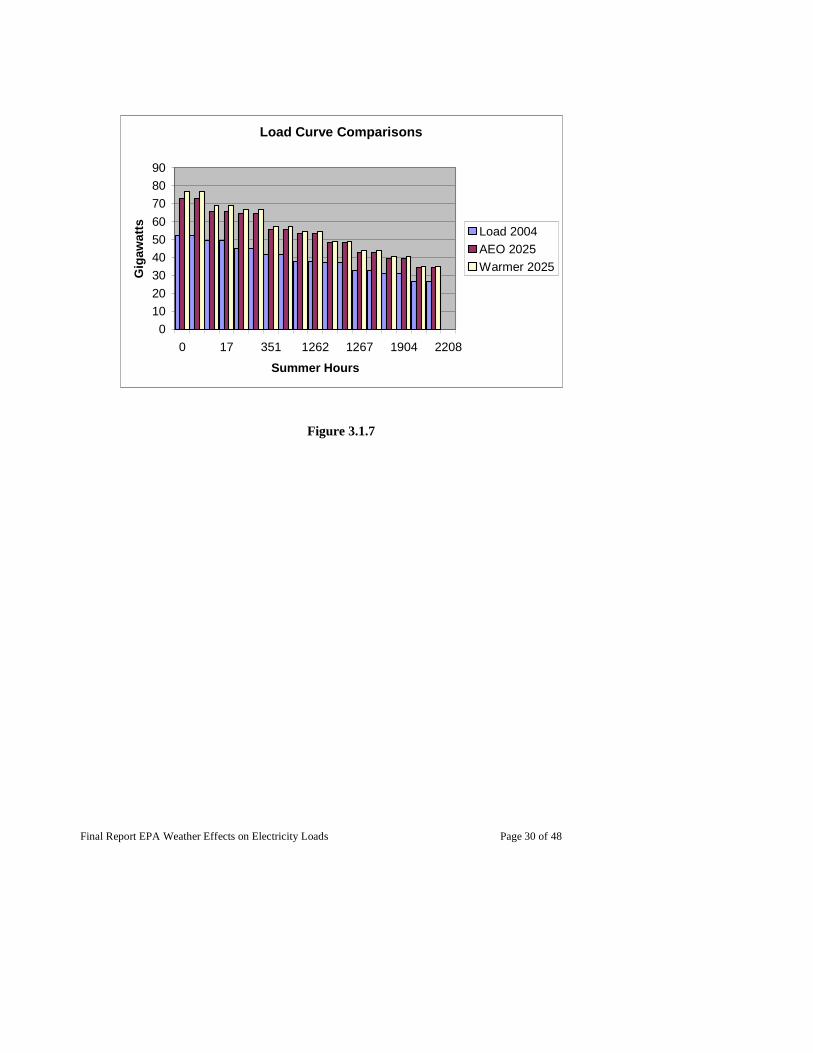
Our hypothesis was that warmer weather would change the annual pattern or shape of the load from winter to summer. In addition, the implied daily load could change more toward peaking periods. This was observed in the short-run models. Higher temperatures will reduce residential and commercial demand for space heating in the winter and increase the demand for space cooling in the summer. The former is typically supplied by fossil fuels while the later is almost exclusively provided by electricity. The impact could lead to greater relative peaking capacity needs, particularly in the summer. Table 3.1.2 presents the results from the Comparison for PJM (MAAC) Summer Load Slice with warming climate change scenario. The first four columns categorize the nine slices of the load curve. Load groups 7,8, and 9 refer to the midday, morning and evening, and night-time hours respectively. These are the hours 8-18, 6-7 and 19-24, and 1-5 respectively. There is a further breakdown by load group into three segments relating to the percent of load expected in each group. The breakdown is into top 1% or peak load in the group, the next 33%, and finally the 66% lowest expected load in each (time) group. These are the three load segments 1,2, and 3 respectively. Column four presents the total number of hours for the summer load in load slice. The load in Gigawatts for 2004 is given in column 5 followed by the NEMS reference projection for 2025 and then the projection for 2025 in the climate change scenario. This is followed by the percent change in the loads in 2025 from the 2004 in the next two columns. The percent increase over the NEMS reference case by load slice for the climate warming scenario. The last two columns show the annual percent increase in loads by for the NEMS and warming scenarios from 2004. The impact of temperature warming in the summer scenario had two important effects. First, average load demand is about 2.7 percent higher in the summer months than in the NEMS reference case. Second, the load demand is not proportionately higher by load slice. Peak demand was 5.4 percent higher in the climate warming scenario. Thus, the results suggest an important impact on the load shape. Climate change will have a disproportionate effect on load in the peak periods in each load group. This may be exactly the periods when ozone is likely to be more of a problem. Figure 3.1.7 illustrates the impacts in a bar chart with three bars in each section showing the 2004 load, 2025 NEMS reference load, and the 2025 climate change scenario.


Table 3.1.2

Summer Load Slice Comparison for PJM (MAAC)

Load GigaWatts Percent Change from 2004

Annual Percent Change 2004

Slice Load Group

Load Segment

Hours 2004 Reference 2025

Warmer 2025

Reference Warmer

Percent Increase

Over Reference

Case Reference Warmer

1 7 1 10.1 52.5 73.1 77.08 39.19% 46.68% 5.38% 1.59%

2 8 1 7.4 49.5 65.8 69.05 32.75% 39.41% 5.02% 1.36%

3 7 2 334.0 45.3 64.5 66.84 42.45% 47.70% 3.68% 1.70%

4 8 2 242.9 41.9 55.6 57.36 32.80% 37.04% 3.19% 1.36%

5 7 3 667.9 37.6 53.1 54.58 41.05% 44.99% 2.79% 1.65%

6 9 1 4.6 37.2 48.1 49.10 29.45% 32.01% 1.98% 1.24%

7 8 3 485.8 33.0 43.0 43.82 30.08% 32.71% 2.02% 1.26%

8 9 2 151.8 30.8 39.6 40.31 28.75% 30.97% 1.72% 1.21%

9 9 3 303.6 26.8 34.5 34.98 28.87% 30.78% 1.48% 1.22%

2004 Load is an estimate for the base year of the Annual Energy Outlook 2005 Source: EIA

Reference 2025 Load is the Reference Case for the Annual Energy Outlook 2005 Source: EIA Warmer 2025 Load is an estimate for the impact of an increase in CDD for PJM (MAAC) region. The 30 year population weighted average was about 800. The scenario considers a case where the average of the 5 warmest years in the region is used. The estimate was 950.

Acknowledgements: John Cymbalsky (EIA), Laura Martin (EIA), and Frank Morra (Booz Allen Hamilton)


Load Curve Comparisons

0

10

20

30

40

50

60

70

80

90

0 17 351 1262 1267 1904 2208

Summer Hours

Gig

awat

ts Load 2004AEO 2025Warmer 2025

Figure 3.1.7


Section 3.2 The RSTEM Description and Temperature Elasticities A second model, also from EIA, the Regional Short-Term Energy Model (RSTEM) estimates regional electricity consumption by sector was used as a complement to the analysis. It is a short-term econometric forecasting model by region and sector and is part of EIA’s new Regional Short Term Energy Outlook. While the forecasting model is focused on a horizon of 1 quarter to two years, the electricity consumption model is a dynamic one. Thus long-run price, income, cooling degree day and heating degree day elasticities can be calculated. The temperature sensitivities from this model can be roughly compared with the long-run model results from the NEMS.

We developed this model with the support of David Costello, Office of Energy Markets and End Use (EMEU), EIA, U.S. Department of Energy. We realized the complementary nature of this research on the EPA STAR grant. The temperature sensitivities from this model can be roughly compared with the long-run model results from the NEMS. Below we 1) briefly describe the econometric issues, 2) summarize the sector specific models, 3) provide detailed descriptions of the residential and commercial equations, and 4) present the short-run and long run elasticity estimates. The data for the model is briefly described in Appendix 3.

Section 3.2.1 Econometric Modeling Issues

The time series energy-econometric consumption models are designed to provide analytical and forecasting support by the nine U.S. Census Regions and four particular states (California, Florida, New York, and Texas). Sectoral electricity demand equations are developed for the residential, commercial, and industrial sectors. The demand equations are based on time series energy econometric techniques. The specifications address issues related to dynamics, stationarity, integration, cointegration, seasonality, and structural breaks. The consumption equations are aggregated into regional models and nationally by sector.

Figures 3.1.8 present the monthly (population weighted) CDD and HDD values for the period 1990-2004. The residential and commercial consumption loads per month per day are provided in Figure 3.1.9 respectively. There are clear seasonal peaks in the two series. In addition, the data show the impact of trends related to economic activity, population growth, and energy consumption. Also, the commercial sector data illustrate the potential for fluctuations due to economic activity.

The RSTEM_EC were developed using the principles of the general-to-specific modeling approach advocated by Hendry (1986a, 1986b, 1993, 1995, and 2000). The general-to-specific modeling approach is a relatively recent strategy used in econometrics. (See Appendix 4.) It attempts to characterize the properties of the sample data in simple parametric relationships, which remain reasonably constant over time, account for the findings of previous models, and are interpretable in an economic and financial sense. Rather than using econometrics to illustrate theory, the goal is to "discover" which alternative theoretical views are tenable and test them scientifically.


0

100

200

300

400

94 95 96 97 98 99 00 01 02 03 04

Cooling

0

200

400

600

800

1000

1200

1400

1600

94 95 96 97 98 99 00 01 02 03 04

Heating

Monthly CDD and HDD for the Mid-Atlantic (PJM) Region

Figure 3.1.8


12

14

16

18

20

22

24

26

28

94 95 96 97 98 99 00 01 02 03 04

RESIDENTIAL

14

16

18

20

22

24

26

94 95 96 97 98 99 00 01 02 03 04

COMMERCIAL

Residential and Commercial Electricity ConsumptionMid-Atlantic Region

Bill

ions

of K

WH

per

Mon

th p

er D

ay

Figure 3.1.9


Section 3.2.2 Summary of Sector Specific Models Residential Demand: There are economic, seasonal, and trend issues which need to be addressed in the residential models. The primary determinants of residential electricity demand in a region are: occupied housing units or households; share of occupied housing units or households using electricity as the primary energy source for heating; share of occupied housing units or households with installed air conditioning; cooling degree-days; heating degree-days; real delivered residential per-unit electricity charges; real personal income per household. Commercial Demand: The primary determinants of commercial electricity demand in a region are: employment, hours worked or real wage disbursements in commercial employment (as a proxy for commercial sector output); cooling degree-days; heating degree-days; real commercial-sector per-unit delivered electricity charges; self-generating capacity in the commercial sector. Autonomous trends in commercial electricity use intensity are additional factors in commercial demand related to commercial building shell efficiencies, average commercial floor-space per unit of output, and penetration of electricity-using equipment in commercial establishments. Industrial Demand: The primary determinants of industrial electricity demand in a region are: employment, hours worked or real wage disbursements in industrial employment or industrial output as measured by the Federal Reserve Board; real industrial-sector per unit delivered electricity charges; cooling degree-days; heating degree-days; self-generating capacity in the industrial sector. Autonomous trends in industrial electricity use intensity are additional factors in industrial demand related to energy efficiency trends in industrial processes and equipment, shifts in regional industrial output patterns among industry sectors of varying levels of electricity use intensity per unit of output, and penetration of general electricity-using equipment in industrial establishments. Other Demand: Other electricity demand in a region, which consists of electricity sales not designated as residential, commercial or industrial (municipal lighting and other general service as well as transportation, for examples), is assumed to be determined by general growth of economic activity in the region, as measured by gross regional product or other aggregate activity measures. Also seasonal factors are important determinants of demand in certain regions. The above-listed demands for electricity relate to retail sales, or sales distributed by local distribution companies, either for own account or for the account of independent service providers. Two other demand components are: electricity generated by and consumed by an entity or facility, such as an industrial establishment (with either combined heat and power (CHP) or electric-only generating capability) or a commercial facility such as a University or other non-industrial facility; electricity generated by one entity and delivered directly to another entity, by-passing retail distribution. The bulk of such non-retail demand is in the industrial sector (approximately 2 percent in 2002). In RSTEM, the non-retail component of electricity demand is treated separately and at the national level. The consumption equations are specified in terms of MWHR per day per month. The generic regional model with the sectoral components or modules can be represented as:

��¶��


( ) / ( / , / ; , ,

, , )

( ) ( / , , , , ,

, , , )

( ) ( / , , , , ,

, , , ,

( )

r r

c c

i i

o

A L EXRCP HH f ESRCU CPI PY HH PrO PNG

Eshr HDD CDD

A L EXCMCP f ESCMU CPI GSP EESPP CW Cshr

PrO PNG HDD CDD

A L EXICP f ESICU WPI IP EESPP GSP CW

Cshr PrO PNG HDD

A L EXOTP

� �� =� ��

)

( / , ; , )

.

r

c

i

o o

e

e

eCDD

f ESOTU WPI GSP HDD CDD e

EXTCP EXRCP EXCMP EXICP EXOTP

� � � �� +� � � ��

= + + +

There are four estimated equations and one identity for total consumption. The equations are time series models. For example, the A(L) terms can imply both regular and seasonal autoregressive components. Lags of the right hand side variables are included in the specification as well. Appendix 3 contains a glossary of the variables in the specification. Section 3.2.3 Detailed Descriptions of the Residential and Commercial Equations The residential electricity consumption demand models are estimated using ordinary least squares. Aggregate sales in BkWh in a month are divided by the number of days in the month. The dependent variable is in terms of daily consumption (EXRCP) per household (QHALLC). These two transformations are based on intuitive reasoning and help control for heteroscedasticity in the monthly models. Households are thought to reflect the number of customers. A different equation is estimated for each region and the particular states. They have similar features, but vary for reasons related to geographical location, weather, and access to substitute energy sources like natural gas and heating oil. Below is a generic description of the residential consumption per household per day equations. The residential consumption series has two distinctive time series properties in most regions. There are two seasonal cycles per year, one for cooling in the summer and the other for heating in the winter. The nature of the cycles and their peaks differ. In addition, there appears to be some trend in the consumption series. The specification of the RSTEO-EC equations differs from the current aggregate level STEO model in that seasonal dummy variables and a deterministic time trend are not included in the equations. Consumption per household per day is transformed into natural logarithms. The residential consumption series is non-stationary. There is a question of whether the series are integrated and what the appropriate specification is. This version of the RSTEM treats the order integration as following an annual seasonal cycle6. The data is first transformed into natural logarithms and then the first difference at the annual frequency is calculated. This appears to produce a stationary series for modeling. The consumption series are obtained from reported monthly sales, but are not strictly related to consumption in the month they are reported. Reported sales are based on an as- reported basis by billing cycle

6 Unit root tests for a sample of series were performed at both the zero and annual frequency were performed and appear to support this specification. A more thorough analysis of the data is expected in future versions of the model.


rather than calendar months. Thus a particular month’s electricity sales volume represents consumption by customers for the current month and part for the previous month. Electricity prices per kWh (ESRCU) are entered in the models with a one-month lag to more accurately reflect the prices that consumers know they paid. The data is first transformed into natural logarithms and then the first difference at the annual frequency is calculated. Several regions had a sizable portion of households using natural gas (NGRCU) for heating and hot water use based on the Residential Energy Consumption Survey. This survey also shows that heating oil (D2RCUUS) was an important heating fuel in the Northeast. The prices of natural gas and heating oil were tested in these equations. The Consumer Price Index (CPI2000) is used to deflate the retail price series unless otherwise specified, to remove inflation effects. Population weighted cooling degree-day and heating degree-day series, ZWCD and ZWHD respectively, are used to capture weather effects. They are incorporated in the equation specification in three ways. First, the annual change in the number of cooling and heating degree-days is consistent with the annual difference of the dependent variable. The actual level is considered as well. In addition, the degree-day measures are interacted with the price series for several regions to capture the joint sensitivity to these series. Household real disposable income (PY) effects on a monthly basis are assumed to be small, if not zero. The nominal disposable personal income series is deflated by the Consumer Price Index (CPI2000). Annual changes in income per household were included in the models, but for the most part did not provide explanatory power. Also, real disposable income is included in a budget share term to capture a possible long run or error correction component to consumption demand. The specifications for every region included an electricity budget share variable. The budget share is calculated as the monthly household electric bill divided by the household disposable income, (EXRCP* ESRCU* ZSAJQUS)/PY. Consumption per day is rescaled by the days per month to obtain total sales. This expression is appealing from economic theory. Also, it is consistent with an error correction representation for integrated series and the concept of cointegration. Households have a desired or equilibrium budget share allocated to electricity services. If expenditures exceed that level or share, because of higher prices or a fall in income, this will slow down the growth in consumption of electricity. The budget share measure was considered at the one- month and one-year lag; in some cases the change in budget share over the previous year provided a valid simplification. The annual lag appears to be the more important in general. Monthly dummy variables are not used in the residential consumption models, because the effects are accounted for through the annual differencing and use of the cooling degree-day and heating degree-day variables. However, dummy variables have been incorporated to capture outlier effects from severe weather and possible measurement error in the data. The commercial electricity consumption demand models are estimated using ordinary least squares. Aggregate sales in X BkWh are divided by the number of days in the month. The dependent variable is in terms of daily consumption (EXCMP=EXCM/ZSAJQUS). A different equation is estimated for each region and the individual states. They have similar features, but will vary for reasons related to geographical location, economic activity, weather, and access to substitute energy sources like natural gas. Below is a generic description of the commercial consumption per day equations. The primary determinants of commercial electricity demand in a region are: employment and or real


wage disbursements in commercial employment (as a proxy for commercial sector output); cooling degree-days; heating degree-days; real industrial-sector per-unit delivered electricity charges, and natural gas prices. The commercial consumption series has two distinctive time series properties in most regions similar to the residential series, but perhaps not as pronounced. There are two seasonal cycles per year, one for cooling and the other for heating in the winter. The nature of the cycles and their peaks differ. In addition, there appears to be some trend in the consumption series. The commercial consumption series are non-stationary. There is a question of whether the series are integrated and what the appropriate specification is. This version of the RSTEM-EC treats most regions with the order of integration as following an annual seasonal cycle7. The data is first transformed into natural logarithms and then the first difference at the annual frequency is calculated. This appears to produce a stationary series for modeling. There may be 1-2 exceptions where only a first difference is used. Real Electricity prices per kWh (ESICU) are entered in the models with a one-month lag to more accurately reflect the prices that consumers know they paid. The data is first transformed into natural logarithms and then the first difference at the annual frequency is calculated. Several regions had a sizable portion of commercial firms using natural gas (NGRCU) according to the Commercial Buildings Energy Consumption Survey. The retail energy price series are deflated by the Consumer Price Index (CPI2000) or specified in relative terms. Population weighted cooling degree-day and heating degree-day series, ZWCD and ZWHD respectively, are used to capture weather effects. They are incorporated in the equation specification in three ways. First the annual change in the number of cooling and heating degree-days is consistent with the annual difference of the dependent variable. The actual level is considered as well. In addition, the degree-daymeasures are interacted with the price series for several regions to capture the joint sensitivity to these series. There is no direct economic commercial or service sector revenue or expenditure series. The level of employment in the private service sector (EESPPC) serves as a proxy for the level of economic activity in the region. Electricity consumption per worker (EXCMP/EESPPC) is used to capture trends and/or correct for deviations in consumption from “equilibrium” consumption. Another indicator for “equilibrium” consumption is the ratio of electricity expenditures to labor costs ((EXCMP*ESCMU*ZSAJQUS)/ CWDSPPC). This measure attempts to represent firms’ concerns over relative input costs. These expressions are appealing from economic theory. Also, they may be consistent with an error correction representation for integrated series and the concept of cointegration. Both measures were considered in the general model specifications, but often only one was necessary in the specific models. The variables were entered with a one-year lag or as the change over the past year from the previous month. Section 3.2.4 The Short-run and Long-run Elasticity Estimates. The model specifications range from simple autoregressive components with explanatory variables to seasonal differenced models with autoregressive components and explanatory variables. The residential models

7 Unit root tests for a sample of series were performed at both the zero and annual frequency were performed and appear to support this specification. A more thorough analysis of the data is expected in future versions of the model.


dependent variable is in terms of household electricity consumption per day. The commercial sector dependent variable is in terms on consumption per day. Below is a generic specification example in seasonal differences with autoregressive components at lags one and the seasonal lag.

( ) ( ) ( ) ,4

1 ln (2) 1 ln (3) 1 ln ( )

12 , 4,5,6,..., 0,12,3,...,

kS S S S

t t t i t j ti

L y c L L y c L L y c i x

where s i k and j p

ε−=

− = − + − + +

= = =

�

The x variables are explanatory variables like prices, economic activity like income, weather data like heating-degree day and cooling-degree day, and other deterministic variables. The short-run elasticity for an explanatory variable like cooling degree days is given by

, (4) *SY CDD tc CDDη =

The long-run elasticity for cooling degree days is equal to

( ) ( ) ( )4

,

( ) *

1 (2) 1 3 1

k

L iY CDD s s s

c i CDD

c L L c L Lη ==

− − + −

�

Tables 3.2.1 and 3.2.2 present the price and income elasticity estimates and the cooling-degree day and heating-degree day elasticities respectively. Results for the Mid-Atlantic region, East North Central Region, and South Atlantic region are provided, because the include the PJM, ECAR, and SERC regions used in the EPA study respectively.


The signs on the elasticities are as hypothesized and conform to the first and second laws of demand. That is the short-run elasticities are smaller than the long-run elasticities. In the short-run households and businesses cannot immediately respond to an increase in CDD and HDD, because their stock and housing and building shell efficiency and appliances are given. As time progresses however, they adjust their housing and building stocks and energy using appliances stocks. We note that the CDD effects appear larger in the Mid-Atlantic and South Atlantic region than in the East North Central region. This is likely due to the greater summer cooling needs and lower heating needs with a warming temperature.

Table 3.2.1

Regional STEO Elasticity Estimates

Region Price Elasticities Income Elasticities

Short-run Long-run Short-run Long-run

East North Central -0.02 -0.06 0.34 1.04

Mid-Atlantic -0.03 -0.59 0.32 0.72

South Atlantic -0.05 -0.22 0.11 0.47

Table 3.2.2

Regional STEO Elasticity Estimates

Region Cooling Degree Day Elasticities Heating Degree Day Elasticities

Short-run Long-run Short-run Long-run

East North Central 0.05 0.23 0.18 0.37

Mid-Atlantic 0.33 0.56 0.13 0.28

South Atlantic 0.04 0.64 0.11 0.19


Bibliography

Ackerman, G, “Short-term Load Prediction for Electric Utility Control of Generating Units,” in D.W. Bunn and E.D. Farmer, eds. Comparative Models for Electrical Load Forecasting, (1985) Wiley: New York.

Baxter, Lester W., and Kevin Calandri. “Global warming and electricity demand; A study of California.” Energy Policy March (1992): 233-244.

Belzer, David B., Michael J. Scott, Ronald D. Sands. “Climate Change Impacts on U.S. Commercial Building Energy Consumption: An Analysis Using Sample Survey Data.” Energy Sources 18 (1996): 177-201.

Darmstadter, Joel. “Climate change impacts on the energy sector and possible adjustments in the region.” Climatic Change 24 (1993): 117-129.

Electric Power Research Institute, “Forecasting and Modeling Time-of-Day and Seasonal Electricity Demands,” (1977) EPRI EA-578-SR, Palo Alto, CA.

Gupta, P.C., “Adaptive Short-term Forecasting of Hourly Loads Using Weather Information,” in D.W. Bunn and E.D. Farmer, eds. Comparative Models for Electrical Load Forecasting, (1985) Wiley: New York.

Hadley, Stanton W., David J. Erikson III, Jose Luis Hernandez, and Starley Thompson, “Future U.S. Energy Use for 2000-2025 as Computed with a Global Climate Change Prediction Model and Energy Demand Model,” Proceedings of the 24th Annual North American Conference of the USAEE, United States Association for Energy Economics, Cleveland OH.

Harvey, Andrew, Siem Jan Koopmans, “Forecasting Hourly Electricity Demands Using Time-Varying Splines,” Journal of the American Statistical Association, (1993) 88, pp 1228-1237.

Hendry, David F., 1986, " Econometric Modelling with Cointegrated Variables: An Overview," Oxford Bulletin of Economics and Statistics, 48, 3, pp 201-12.

Hendry, David F., and Juselius, Katarina, 2000, “Explaining Cointegration Analysis: Part I,” The Energy Journal, vol. 21, no. 1, pp1-42.

Hendry, D. F., (1986). "Using PC-GIVE in econometrics teaching" Oxford Bulletin of Economics and Statistics, 48, 87--98.

Hendry, D. F.,(1993). Econometrics: Alchemy or Science? Oxford: Blackwell Publishers.

Hendry, D. F., (1995). Dynamic Econometrics. Oxford: Oxford University Press.

Hobbs, Benjamin F. (2001). “Linear Complementarity Models of Nash-Cournot Competition in Bilateral and POOLCO Power Markets.” IEEE Transactions on Power Systems , vol. 16.2, pp194-202.

Hobbs, Benjamin F., Carolyn B. Metzler, and Jong-Shi Pang. (2000). “Strategic Gaming Analysis for Electric Power Systems: An MPEC Approach.” IEEE Transactions on Power Systems ,Volume 15, 2.


Hobbs, Benjamin F., et al. “Artificial neural networks for short-term energy forecasting: Accuracy and economic value.” Neurocomputing 23 (1998): 71-84.

Holtedahl, Pernhille and Frederick Joutz, "Residential Electricity Demand in Taiwan: A Error Correction Approach," Energy Economics, 2004, vol. 26 (2) pp 201-224.

Hongyi Li, G. S. Maddala, Frederick Joutz, and Robert Trost, "Estimation of Short Run and Long Run Elasticities of Energy Demand from Panel Data Using Shrinkage Estimators"), Journal of Business and Economics Statistics, Vol. 15, No. 1, January, 1997.

Jaeger, C., G. Dürrenberger, H. Kastenholz, B. Truffer. “Determinants of environmental action with regard to climatic change.” Climatic Change 23 (1993): 193-211.

Joutz, Frederick and Julian Silk, “Short- and Long-Run Elasticities in U.S. Residential Electricity Demand: A Cointegration Approach,” Energy Economics, (August 1997).

Joutz, Frederick and Robert Trost, "Using Stochastic Simulation to Test the Effect of Different Data Seasonal Adjustment on Forecast Standard Errors of Motor Gasoline Demand," International Journal of Forecasting, 1992, volume 8, p219-231.

Leppitsch, Michael J., and Benjamin F. Hobbs. “The Effect of NOx Regulations on Emission Dispatch: A Probabilistic Production Costing Analysis.” IEEE Transactions on Power Systems 11, No. 4 (1996): 1711-1717.

Matsuura, K. “Effects of Climate Change on Building Energy Consumption in Cities.” Theoretical and Applied Climatology 51 (1995): 105-117.

McMenamin, J. Stuart, and Frank A. Monforte. “Short Term Energy Forecasting with Neural Networks.” The Energy Journal 19, No. 4 (1998): 43-61.

Morris III, Samuel C., Gary A, Goldstein, Ajay Sanghi, and Douglas Hill. “Energy Demand and Supply in Metropolitan New York with Global Climate Change.” Annals New York Academy of Sciences Volume (PubDate): 139-150.

National Assessment Synthesis Team (NAST) 2000, Climate Change Impacts on the United States, U.S. Global Change Research Program, Cambridge University Press. [http:www.gcrio.org/NationalAssessment/ondex.html]

Rosenthal, Donald H. and Howard K. Gruenspecht, “Effects of Global Warming on Energy Use for Space Heating and Cooling in the United States,” Energy Journal, 16(2): 77-96.

Ramanathan, Ramu, Robert Engle, Clive W.J. Granger, Farshid Vahid-Araghi, and Casey Bruce, “Short-run Forecasts of Electricity Loads and Peaks,” International Journal of Forecasting, (1997) 13, pp 161-74.

Sailor, David J., and J. Ricardo Muñoz. “Sensitivity of electricity and natural gas consumption to climate in the U.S.A. – Methodology and results for eight states.” Energy 22, No. 10 (1997): 987-998.


Sailor, David J., Jesse N. Rosen, and J. Ricardo Muñoz. “Natural gas consumption and climate: a comprehensive set of predictive state-level models for the United States.” Energy the International Journal, 23, No. 2 (1998): 91-103.

Schneider, A.M. and T. Takenawa and D.A. Schiffman, “24-Hour Electric Load Forecasting,” ,” in D.W. Bunn and E.D. Farmer, eds. Comparative Models for Electrical Load Forecasting, (1985) Wiley: New York.

Scott, Michael J., Laura E. Wrench, and Donald L. Hadley. “Effects of Climate Change on Commercial Building Energy Demand.” Energy Sources 16 (1994): 317-332.


Appendix 1: Summer Hypotheses

logLoad(i) C Tue Wed Thu Fri Sat Sun Holiday Jul Au g Sep Jun°F Jul°F Aug°F Sep°F Jun°F^2 Jul°F^2 Aug°F^2 Sep°F^2 Jun°F^3 Jul°F^3 Aug°F^3 Sep°F^3 logLoad(i-1) logLoad(i-2) logLoad(i-3) logLoad(i-24 )

Restricted Models SpecificationH0:1 There are no Day or Holiday effects Tue = Wed = Thu = Fri = Sat = Sun = Holiday = 0H0:2 There are no Weekend or Holiday effects Sat = Sun = Holiday = 0H0:3 There are no Weekend effects Sat = Sun = 0H0:4 There are no Sunday or Holiday Effects Sun = Holiday = 0H0:5 There are no Weekend effects; Weekday effects are a ll the same Sat = Sun = 0; Tue = Wed = Thu = FriH0:6 There are no Month effects Jul = Aug = Sep = 0H0:7 There are no Day or Holiday or Month effects Tue = Wed = Thu = Fri = Sat = Sun = Holiday = Jul = Aug = Sep = 0H0:8 There are no Weekend or Holiday or Month effects Sat = Sun = Holiday = Jul = Aug = Sep = 0H0:9 There are no Weekend or Month effects Sat = Sun = Jul = Aug = Sep = 0H0:10 There are no Sunday or Holiday or Month Effects Sun = Holiday = Jul = Aug = Sep = 0H0:11 There are no Weekend or Month effects; Weekday effe cts are all the same Sat = Sun = Jul = Aug = Sep = 0; Tue = Wed = Thu = FriH0:12 There are no Weekday effects Tue = Wed = Thu = Fri = 0H0:13 There are no Weekday or Month effects; Weekend and Holiday effects are the same Tue = Wed = Thu = Fri = Jul = Aug = Sep = 0; Sat = Sun = HolidayH0:14 There are no Temp Level effects Jun °F = Jul °F = Aug °F = Sep °F = 0H0:15 There are no Temp Level effects for June or Septemb er Jun °F = Sep °F = 0H0:16 There are no Temp Level effects for June Jun °F = 0H0:17 There are no Temp Level effects for September Sep °F = 0

H0:18 There are no Temp Level effects for September; Temp Level effects for other months are all equalSep °F = 0; Jun °F = Jul °F = Aug °F

H0:19 There are no Temp Level effects for June; Temp Leve l effects for other months are all equal Jun °F = 0; Jul °F = Aug °F = Sep °F

H0:20There are no Temp Level effects for June or Septemb er; Temp Level effects for July and August are equal Jun °F = Sep °F = 0; Jul °F = Aug °F

H0:21 Temp Level effects for June and September are equal; Temp Level effects for July and August are e qualJun °F = Sep °F; Jul °F = Aug °F

H0:22 Temp Level effects for all months are equal Jun °F = Jul °F = Aug °F = Sep °FH0:23 There are no Temp Squared effects Jun °F^2 = Jul °F^2 = Aug °F^2 = Sep °F^2 = 0H0:24 There are no Temp Squared effects for June or Septe mber Jun °F^2 = Sep °F^2 = 0H0:25 There are no Temp Squared effects for June Jun °F^2 = 0H0:26 There are no Temp Squared effects for September Sep °F^2 = 0

H0:27 There are no Temp Squared effects for Septembe r; Temp Squared effects for other months are all eq ualSep °F^2 = 0; Jun °F^2 = Jul °F^2 = Aug °F^2

H0:28 There are no Temp Squared effects for June; Te mp Squared effects for other months are all equalJun °F^2 = 0; Jul °F^2 = Aug °F^2 = Sep °F^2

H0:29There are no Temp Squared effects for June or Septe mber; Temp Squared effects for July and August are equal Jun °F^2 = Sep °F^2 = 0; Jul °F^2 = Aug °F^2

H0:30Temp Squared effects for June and September are equ al; Temp Squared effects for July and August are equal Jun °F^2 = Sep °F^2; Jul °F^2 = Aug °F^2

H0:31 Temp Squared effects for all months are equal Jun °F^2 = Jul °F^2 = Aug °F^2 = Sep °F^2

H0:32 There are no Temp Level or Squared effectsJun °F = Jul °F = Aug °F = Sep °F = Jun °F^2 = Jul °F^2 = Aug °F^2 = Sep °F^2 = 0

H0:33 There are no Temp Level or Squared effects for June or September Jun °F = Sep °F = Jun °F^2 = Sep °F^2 = 0H0:34 There are no Temp Level or Squared effects for June Jun °F = Jun °F^2 = 0H0:35 There are no Temp Level or Squared effects for Sept ember Sep °F = Sep °F^2 = 0

H0:36 There are no Temp Level or Squared effects for September; Temp effects for other months are all e qualSep °F = 0; Jun °F = Jul °F = Aug °F; Sep °F^2 = 0; Jun °F^2 = Jul °F^2 = Aug °F^2

H0:37 There are no Temp Level or Squared effects for June; Temp effects for other months are all equalJun °F = 0; Jul °F = Aug °F = Sep °F; Jun °F^2 = 0; Jul °F^2 = Aug °F^2 = Sep °F^2

H0:38There are no Temp Level or Squared effects for June or September; Temp effects for July and August are equal

Jun °F = Sep °F = 0; Jul °F = Aug °F; Jun °F^2 = Se p °F^2 = 0; Jul °F^2 = Aug °F^2

H0:39 Temp effects for June and September are equal; Temp effects for July and August are equalJun °F = Sep °F; Jul °F = Aug °F; Jun °F^2 = Sep °F ^2; Jul °F^2 = Aug °F^2

H0:40 Temp effects for all months are equalJun °F^2 = Jul °F^2 = Aug °F^2 = Sep °F^2; Jun °F^2 = Jul °F^2 = Aug °F^2 = Sep °F^2

H0:41 No Cubic Effects Jun °F^3 = Jul °F^3 = Aug °F^3 = Sep °F^3 = 0H0:42 No Jun/Sept Cubic Effects Jun °F^3 = Sep °F^3 = 0H0:43 Cubic Effects for Jun = Sep; Jul = Aug Jun °F^3 = Sep °F^3; Jul °F^3 = Aug °F^3H0:44 Cubic Effects are the same across all months Jun °F^3 = Jul °F^3 = Aug °F^3 = Sep °F^3

H0:45 No Squared/Cubic EffectJun °F^2 = Jul °F^2 = Aug °F^2 = Sep °F^2 = Jun °F^ 3 = Jul °F^3 = Aug °F^3 = Sep °F^3 = 0

H0:46 No Jun or Sep Squared/Cubic Effects Jun °F^2 = Sep °F^2 = Jun °F^3 = Sep °F^3 = 0

H0:47 Squared/Cubic Effects for Jun = Sep; Jul = AugJun °F^2 = Sep °F^2; Jul °F^2 = Aug °F^2; Jun °F^3 = Sep °F^3; Jul °F^3 = Aug °F^3

H0:48 Squared/Cubic Effects are the same in all mont hsJun °F^2 = Jul °F^2 = Aug °F^2 = Sep °F^2; Jun °F^3 = Jul °F^3 = Aug °F^3 = Sep °F^3

H0:49 No Level/Squared/Cubic EffectsJun °F = Jul °F = Aug °F = Sep °F = Jun °F^2 = Jul °F^2 = Aug °F^2 = Sep °F^2 = Jun °F^3 = Jul °F^3 = Aug °F^3 = Sep °F^3 = 0

H0:50 No Jun or Sep Level/Squared/Cubic Effects Jun °F = Sep °F = Jun °F^2 = Sep °F^2 = Jun °F^3 = Sep °F^3 = 0

Unrestricted Model


Appendix 2: Winter Hypotheses

logLoad(i) C Tue Wed Thu Fri Sat Sun Holiday Feb Ma r Dec Jan°F Feb°F Mar°F Dec°F Jan°F^2 Feb°F^2 Mar°F^2 Dec°F^2 Jan°F^3 Feb°F^3 Mar°F^3 Dec°F^3 logLoad(i-1) logLoad(i-2) logLoad(i-3) logLoad(i-24 )

Restricted Models SpecificationH0:1 There are no Day or Holiday effects Tue = Wed = Thu = Fri = Sat = Sun = Holiday = 0H0:2 There are no Weekend or Holiday effects Sat = Sun = Holiday = 0H0:3 There are no Weekend effects Sat = Sun = 0H0:4 There are no Sunday or Holiday Effects Sun = Holiday = 0H0:5 There are no Weekend effects; Weekday effects are a ll the same Sat = Sun = 0; Tue = Wed = Thu = FriH0:6 There are no Month effects Feb = Mar = Dec = 0H0:7 There are no Day or Holiday or Month effects Tue = Wed = Thu = Fri = Sat = Sun = Holiday = Feb = Mar = Dec = 0H0:8 There are no Weekend or Holiday or Month effects Sat = Sun = Holiday = Feb = Mar = Dec = 0H0:9 There are no Weekend or Month effects Sat = Sun = Feb = Mar = Dec = 0H0:10 There are no Sunday or Holiday or Month Effects Sun = Holiday = Feb = Mar = Dec = 0H0:11 There are no Weekend or Month effects; Weekday effe cts are all the same Sat = Sun = Feb = Mar = Dec = 0; Tue = Wed = Thu = FriH0:12 There are no Weekday effects; Weekend and Holiday e ffects are the same Tue = Wed = Thu = Fri = 0, Sat = Sun = HolidayH0:13 There are no Weekday or Month effects; Weekend and Holiday effects are the same Tue = Wed = Thu = Fri = Feb = Mar = Dec = 0; Sat = Sun = HolidayH0:14 There are no Temp Level effects Jan °F = Feb °F = Mar °F = Dec °F = 0H0:15 There are no Temp Level effects for March or Decemb er Mar °F = Dec °F = 0H0:16 There are no Temp Level effects for December Dec °F = 0H0:17 There are no Temp Level effects for March Mar °F = 0

H0:18 There are no Temp Level effects for December; Temp Level effects for other months are all equalDec °F = 0; Jan °F = Feb °F = Mar °F

H0:19 There are no Temp Level effects for March; Temp Lev el effects for other months are all equal Mar °F = 0; Feb °F = Mar °F = Dec °F

H0:20There are no Temp Level effects for March or Decemb er; Temp Level effects for January and February are equal Mar °F = Dec °F = 0; Jan °F = Feb °F

H0:21Temp Level effects for March and December are equal ; Temp Level effects for January and February are equal Mar °F = Dec °F; Jan °F = Feb °F

H0:22 Temp Level effects for all months are equal Jan °F = Feb °F = Mar °F = Dec °FH0:23 There are no Temp Squared effects Jan °F^2 = Feb °F^2 = Mar °F^2 = Dec °F^2 = 0H0:24 There are no Temp Squared effects for March or Dece mber Mar °F^2 = Dec °F^2 = 0H0:25 There are no Temp Squared effects for March Mar °F^2 = 0H0:26 There are no Temp Squared effects for December Dec °F^2 = 0

H0:27 There are no Temp Squared effects for December ; Temp Squared effects for other months are all equ alDec °F^2 = 0; Jan °F^2 = Feb °F^2 = Mar °F^2

H0:28 There are no Temp Squared effects for March; T emp Squared effects for other months are all equal Mar °F^2 = 0; Jan °F^2 = Feb °F^2 = Mar °F^2

H0:29There are no Temp Squared effects for March or Dece mber; Temp Squared effects for January and February are equal Mar °F^2 = Dec °F^2 = 0; Jan °F^2 = Feb °F^2

H0:30Temp Squared effects for March and December are equ al; Temp Squared effects for January and February are equal Mar °F^2 = Dec °F^2; Jan °F^2 = Feb °F^2

H0:31 Temp Squared effects for all months are equal Jan °F^2 = Feb °F^2 = Mar °F^2 = Dec °F^2

H0:32 There are no Temp Level or Squared effectsJan °F = Feb °F = Mar °F = Dec °F = Jan °F^2 = Feb °F^2 = Mar °F^2 = Dec °F^2 = 0

H0:33 There are no Temp Level or Squared effects for Marc h or December Mar °F = Dec °F = Mar °F^2 = Dec °F^2 = 0H0:34 There are no Temp Level or Squared effects for Dece mber Dec °F = Dec °F^2 = 0H0:35 There are no Temp Level or Squared effects for Marc h Mar °F = Mar °F^2 = 0

H0:36 There are no Temp Level or Squared effects for December; Temp effects for other months are all eq ualDec °F = 0; Jan °F = Feb °F = Mar °F; Dec °F^2 = 0; Jan °F^2 = Feb °F^2 = Mar °F^2

H0:37 There are no Temp Level or Squared effects for March; Temp effects for other months are all equalMar °F = 0; Jan °F = Feb °F = Dec °F; Mar °F^2 = 0; Mar °F^2 = Feb °F^2 = Dec °F^2

H0:38There are no Temp Level or Squared effects for Marc h or December; Temp effects for January and February are equal

Mar °F = Dec °F = 0; Jan °F = Feb °F; Mar °F^2 = De c °F^2 = 0; Jan °F^2 = Feb °F^2

H0:39 Temp effects for March and December are equal; Temp effects for January and February are equal Jan °F = Feb °F; Mar °F^2 = Dec °F^2; Jan °F^2 = Fe b °F^2

H0:40 Temp effects for all months are equalJan °F^2 = Feb °F^2 = Mar °F^2 = Dec °F^2; Jan °F^2 = Feb °F^2 = Mar °F^2 = Dec °F^2

H0:41 No Cubic Effects Jan °F^3 = Feb °F^3 = Mar °F^3 = Dec °F^3 = 0H0:42 No Jan/Dec Cubic Effects Jan °F^3 = Dec °F^3 = 0H0:43 Cubic Effects for Jan = Dec, Feb = Mar Jan °F^3 = Dec °F^3; Feb °F^3 = Mar °F^3H0:44 Cubic Effects are the same across all months Jan °F^3 = Feb °F^3 = Mar °F^3 = Dec °F^3

H0:45 No Squared/Cubic EffectJan °F^2 = Feb °F^2 = Mar °F^2 = Dec °F^2 = Jan °F^ 3 = Feb °F^3 = Mar °F^3 = Dec °F^3 = 0

H0:46 No Jan or Dec Squared/Cubic Effects Jan °F^2 = Dec °F^2 = Jan °F^3 = Dec °F^3 = 0

H0:47 Squared/Cubic Effects for Jan = Dec; Feb = MarJan °F^2 = Dec °F^2; Feb °F^2 = Mar °F^2; Jan °F^3 = Dec °F^3; Feb °F^3 = Mar °F^3

H0:48 Squared/Cubic Effects are the same in all mont hsJan °F^2 = Feb °F^2 = Mar °F^2 = Dec °F^2; Jan °F^3 = Feb °F^3 = Mar °F^3 = Dec °F^3

H0:49 No Level/Squared/Cubic EffectsJan °F = Feb °F = Mar °F = Dec °F = Jan °F^2 = Feb °F^2 = Mar °F^2 = Dec °F^2 = Jan °F^3 = Feb °F^3 = Mar °F^3 = Dec °F^3 = 0

H0:50 No Jan or Dec Level/Squared/Cubic Effects Jan °F = Dec °F = Jan °F^2 = Dec °F^2 = Jan °F^3 = Dec °F^3 = 0

Unrestricted Model


Appendix 3. RSTEM Data Sources and Descriptions

The historical energy data used to estimate the model come primarily from the IMDS electronic database. IMDS merges data regularly reported in several EIA publications: Petroleum Supply Monthly, Petroleum Marketing Monthly, Electric Power Monthly, Natural Gas Monthly, and Monthly Energy Review. Because of data limitations there are inconsistencies in the level of dis-aggregation of each type of fuel. For example, electricity and natural gas demands are represented by market sector, but petroleum products are generally represented only as national totals or for a combination of sectors (distillate and residual fuel oil are exceptions). Market-level data are available for the regulated industries (electricity and natural gas) while product-level data are available for the petroleum product markets, particularly for data frequencies higher than annual.

These energy price and volume data are supplemented by data from outside sources; the most common are listed below.

• Employment and Earnings, Bureau of Labor Statistics, U.S. Department of Labor. • Industrial Production, Board of Governors, U.S. Federal Reserve System. • Monthly Labor Review, Bureau of Labor Statistics, U.S. Department of Labor. • Monthly State, Regional, and National Heating/Cooling Degree-Days Weighted by

Population, National Oceanic and Atmospheric Administration, U.S. Department of Commerce.

• National Income and Product Accounts of the United States, Bureau of Economic Analysis, U.S. Department of Commerce.

• Survey of Current Business, Bureau of Economic Analysis, U.S. Department of Commerce.

Most of the data sources provide monthly data and are used directly. Quarterly data are interpolated into monthly series. These data are primarily for macroeconomic variables in the national income and product accounts and gross state domestic product accounts.


Simple Glossary of Terms

Acronyms Description EXRCP Residential electricity consumption per day

EXCMP Commercial electricity consumption per day

EXICP Industrial electricity consumption per day

EXOTP Other electricity consumption per day

EXTCP Total electricity consumption per day

HH Number of households

ESRCU Residential retail electricity per kWh

ESCMU Commercial retail electricity per kWh ESICU Industrial retail electricity per kWh ESOTU Other retail electricity per kWh

PY Disposable personal income

CPI Consumer price index: urban households, Base 2000

PrO Price of home heating oil, $/gallon

EShr Electricity expenditure budget share

Cshr Electricity cost per labor costs

EESPP Number of Employees: Commercial or Industrial

GSP Gross State Product: Region-wide or Industrial

IP Industrial Production: Electricity Weighted

CW Wages and Salaries: Commercial or Industrial WPI Wholesale Price Index, Base 2000 PNG Price of Natural Gas

HDD Heating degree-days per month

CDD Cooling degree-days per month


Appendix 4: The General-to-Specific Modeling Approach

The General to Specific Approach follows a set of principles laid out by Haavelmo in 19448. He introduced econometricians to the general principles of analyzing statistical models instead of applying methods. The implication of applying statistical models instead of applying methods is that the researcher should use models based on systems of equations. VARs have a number of advantages in this regard. They allow for dynamic interactions and correlations among variables which is the basis of applied times econometrics. Social scientists definition struggle, because their data does not conform to the hypothetical case knowing the true data generating process. Their data has been collected or simulated in controlled experiments. The applied econometrician must use a probability approach to their craft. We start by assuming a probability structure to the data. This is effectively conjecturing the existence of a data generating process (hereafter DGP).reality the DGP is unknown. The general principles suggest an iterative approach or progressive research strategy.

• Conjecture the DGP • Develop the associated probability theory • Use theory for modeling the empirical evidence • Revise the starting point when the results do not match consistently.

The strategy involves recent development in econometrics known as the Theory of Reduction which motivates the General-to-Specific Approach.

8 Much of the discussion below of Haavelmo’s general principles has benefited from K. Juselius’ applied econometrics book manuscript, chapter 1 Introduction. Oxford University Press expects to publish the book in 2006.

Approaches and or Methodology for Research

Economists Statisticians

Formulate an economically well-specified

model as the empirical model.

Formulate a statistically well-specified

model for the data.

Apply statistical techniques to estimate the

parameters.

Analyze the statistical model to answer the

economic questions of interest.

Methodology for Research

Use statistics passively as a tool to some

derived results.

Statistical model is taken seriously and

used actively as a means of analyzing the

underlying DGP of the economic

phenomenon.


Empirical models are at best approximations of the true data generating process (DGP). The econometric model should exhibit certain desirable properties that render it a valid representation of the true DGP. Hendry (1995) and Mizon (1995) suggest the following six criteria according to the General-to-Specific or LSE methodology.

1. There are identifiable structures in the model that are interpretable in light of economic theory. 2. The residuals must be white noise for the model to be a valid simplification of the DGP. 3. The model must be admissible on accurate observations. For example nominal interest rates and prices

cannot be negative. 4. The conditioning variables are at least weakly exogenous for the parameters of interest in the model.

Forecasting models require strong exogeneity, while policy models require super exogeneity. 5. The parameters of interest must be constant over time and remain invariant to certain classes of

interventions. This relates to the purpose of the model in the previous criteria. 6. The model must be able to explain the results from rival models; it is able to encompass them.

A model that has these six properties is said to be congruent. The sector demand model specification begins by analyzing the time series properties of the energy and economic variables. Autocorrelation functions and partial autocorrelation functions of the series in (log) levels, first differences, and annual differences are examined to look for dynamic patterns and integration. Plots of the series in (log) levels, first differences, annual differences, and monthly seasonal stacks are examined for trends, seasonal effects, shifts in the data generating process, and outliers. Unit root tests are conducted to test for (seasonal) integration and cointegration. The principles and approach have not been fully implemented in the RSTEO modeling effort to-date because of time and resource constraints. But the work is on-going.

weather effects on electricity loads modeling and forecasting

Documents