Weather Adjusting Economic Data

Michael Boldin and Jonathan H. Wright∗

First version: December 18, 2014This version: August 31, 2015

Abstract

This paper proposes and implements a statistical methodology for adjustingemployment data for the effects of deviations in weather from seasonal norms.This is distinct from seasonal adjustment, which only controls for the normalvariation in weather across the year. We simultaneously control for both ofthese effects by integrating a weather adjustment step in the seasonal adjust-ment process. We use several indicators of weather, including temperature andsnowfall. We find that weather effects can be important, shifting the monthlypayrolls change number by more than 100,000 in either direction. The effectsare largest in the winter and early spring months and in the construction sector.A similar methodology is constructed and applied to NIPA data, although themanner in which NIPA data are reported makes it impossible fully to integrateweather and seasonal adjustments.

JEL Classifications: C22, C80Keywords: Weather, employment data, seasonal adjustment, big data.

∗Federal Reserve Bank of Philadelphia, Ten Independence Mall, Philadelphia, PA 19106,michael.boldin@phil.frb.org and Department of Economics, Johns Hopkins University, 3400North Charles St. Baltimore, MD 21218, wrightj@jhu.edu. This is a revised version of an ear-lier manuscript entitled “Weather Adjusting Employment Data”. We are grateful to KatharineAbraham, Roc Armenter, Bob Barbera, Francois Gourio, David Romer, Claudia Sahm, Tom Starkand Justin Wolfers for helpful discussions, and to Natsuki Arai for outstanding research assistance.All errors are our sole responsibility. The views expressed here are those of the authors and donot necessarily represent those of the Federal Reserve Bank of Philadelphia or the Federal ReserveSystem.

1 Introduction

Macroeconomic time series are affected by the weather. For example, in the first

quarter of 2014, real GDP contracted by 0.9 percent at an annualized rate. Com-

mentators and Federal Reserve officials attributed part of the decline to an unusually

cold winter and large snowstorms that hit the East Coast and the South during the

quarter.1 Similarly the slowdown in growth in the first quarter of 2015 was widely

ascribed to another exceptionally harsh winter and other transitory factors. While

the effects of regular variation in weather within a year should, in principle, be taken

care of by the seasonal adjustment procedures that are typically applied to economic

data, these adjustments are explicitly not supposed to adjust for variations that are

driven by deviations from the weather norms for a particular time of year. It is typ-

ically cold in February, depressing activity in some sectors, and seasonal adjustment

controls for this. But seasonal adjustment does not control for whether a particular

February is colder or milder than normal.

Our objective in this paper is to construct and implement a methodology for

estimating how the data would have appeared if weather patterns had followed their

seasonal norms. Monetary policymakers view weather effects as transitory—given

the long and variable lags in monetary policy, they do not generally seek to respond

to weather-related factors. It follows that the economic indicators that they are

provided with ought, as far as possible, be purged of weather effects. Moreover,

we argue that failing to control for abnormal weather effects distorts conventional

seasonal adjustment procedures.

1Prior to the start of the first quarter of 2014, professional forecasters were expecting a seasonallyadjusted increase of around 2.5 percent. The original report for the quarter was 0.1 percent, laterrevised to -2.1 percent, and subsequently revised to -0.9 in the 2015 annual NIPA adjustments thatincluded revisions to the seasonal adjustment process, as discussed in section 4 below. With a snap-back rate of 4.6 percent in the second quarter, it is highly plausible that weather played a significantrole in the decline.

1

The measurement of inflation provides a useful analogy. The Federal Reserve

focuses on core inflation, excluding food and energy, rather than headline inflation.

The motivation is not that food and energy are inherently less important expendi-

tures, but that fluctuations in their inflation rates are transitory. Core inflation is

more persistent, and forecastable, and indeed a forecast of core inflation may be the

best way of predicting overall inflation (Faust and Wright, 2013). In the same way,

economic fluctuations caused by the weather are real, but transitory. We may obtain

a better measure of the economy’s underlying momentum by removing the effects of

abnormal weather.

Economists have studied the effects of the weather on agricultural output for a

long time, going back to the work of Fisher (1925). More recently, they have also

used weather as an instrumental variable (see, for example, Miguel et al. (2004)),

arguing that weather can be thought of as an exogenous driver of economic activ-

ity. Statistical agencies sometimes judgmentally adjust extreme observations due to

specific weather events before applying their seasonal adjustment procedures.2 Al-

though there is a long literature on seasonal adjustment, we are aware of only a

few papers on estimating the effect of unseasonal weather on macroeconomic aggre-

gates. The few papers on the topic include Macroeconomic Advisers (2014), which

regressed seasonally adjusted aggregate GDP on snowfall totals, estimating that snow

reduced 2014Q1 GDP by 1.4 percentage points at an annualized rate, Bloesch and

Gourio (2014) who likewise studied the relationship between weather and seasonally

adjusted data, Dell et al. (2012) who implemented a cross-country study of the effects

of annual temperature on annual GDP, and Foote (2015) who studied weather effects

on state-level employment data. None of these papers integrates weather adjustment

2Even when agencies do this, their goal is just to prevent the anomalous weather from distortingseasonals, not to actually adjust the data for the effects of the weather.

2

in the seasonal adjustment process. This is what the current paper attempts to do.

We focus mainly, but not exclusively, on the seasonal adjustment of the Bureau of

Labor Statistics (BLS) current employment statistics (CES) survey (the “establish-

ment” survey) that includes total nonfarm payrolls. We do so because it is clearly the

most widely followed monthly economic indicator, and also because it is an indicator

for which it is possible for researchers to approximately replicate the official seasonal

adjustment process, unlike for National Income and Product Account (NIPA) data.

We consider simultaneously adjusting these data for both seasonal effects and for

unseasonal weather effects. This can be quite different from ordinary seasonal ad-

justment, especially during the winter and early spring. Month-over-month changes

in nonfarm payrolls are in several cases higher or lower by as much as 100,000 jobs

when using the proposed seasonal-and-weather adjustment rather than ordinary sea-

sonal adjustment. Using seasonal-and-weather adjustment increases the estimated

pace of employment growth in the winters of 2013-2014 and 2014-2015.

The plan for the remainder of this paper is as follows. In Section 2, we discuss

alternative measures of unusual weather and evaluate how they relate to aggregate

employment. This is intended to give us guidance on which weather indicators have

an important impact on employment data. Section 3 describes seasonal adjustment

in the CES and discusses how adjustment for unusual weather effects may be added

into this—seasonal adjustment is implemented at the disaggregate level. Section 4

extends the analysis to NIPA data. Section 5 concludes.

3

2 Measuring unusual weather and its effect on ag-

gregate employment data

We need to construct measures of unseasonal weather that are suitable for adjusting

the CES survey. We first obtained data from the National Centers for Environmental

Information (NCEI) on daily maximum temperatures, precipitation, snowfall and

heating degree days (HDDs) 3 at one station in each of the largest 50 Metropolitan

Statistical Areas (MSAs) by population, in the United States from 1960 to the present.

The stations were chosen to provide a long and complete history of data,4 and are

listed in Table 1. We averaged these across the 50 MSAs, with the averages weighted

by population. MSA population was determined from the 2010 census. This was

designed as a way of measuring U.S.-wide temperature, precipitation and snowfall in

a way that makes a long time series easily available and that puts the highest weight

on areas with the greatest economic activity.5

Let temps denote the actual average temperature on day s, and define the unusual

temperature for that day as temp∗s = temps − 130

Σ30y=1temps,y where temps,y denotes

the temperature on that same day y years previously. Likewise, let prp∗s, snow∗s and

hdd∗s denote the unusual precipitation, snowfall or HDD on day s, relative to the 30-

3The HDD at a given station on a given day is defined as max(18.3-τ, 0) where τ is the averageof maximum and minimum temperatures in degrees Celsius.

4An alternative measure of snowfall, used by Macroeconomic Advisers (2014), is based on adataset of daily county-level snowfall maintained by the NCEI. This clearly has the advantage ofgreater cross-sectional granularity. However, these data only go back to 2005. Our data go muchfurther back, allowing us to construct a longer history of snowfall effects, and to measure normalsnowfall from 30-year averages.

5Weather, of course, varies substantially around the country, and it might seem more natural toadjust state-level employment data for state-level weather effects. We used national-level employ-ment data with national-level weather because the BLS produces state and national data separatelyusing different methodologies. National CES numbers are quite different from the “sum of states”numbers. The reason is that both state and national CES numbers are constructed by survey meth-ods, but the national data uses more disaggregated cells. Meanwhile, it is the national numbersthat garner virtually all the attention from Wall Street and the Federal Reserve.

4

year average. This is in line with the meteorological convention of defining climate

norms from 30-year averages.

In assessing the effect of unusual weather on employment as measured in the

CES, we want to take careful account of the within-month timing of the CES survey.

The CES survey relates to the pay period that includes the 12th day of the month.

Some employers use weekly pay periods, others use biweekly, and a few use monthly.

A worker is counted if (s)he works at any point in that pay period. Cold weather

or snow seems most likely to affect employment status on the day of that unusual

weather, but it is also possible that, for example, heavy snow might affect economic

activity for several days after the snowstorm had ceased. Putting all this together,

temperature/snowfall conditions in the days up to and including the 12th day of the

month are likely to have some effect on measured employment for that month. The

further before the 12th day of the month the unusual weather occurred, the less likely

it is to have affected a worker’s employment status in the pay period bracketing the

12th, and so the less important it should be. But it is hard to know a priori how

to weight unusual weather on different days up to and including the 12th day of the

month. On the other hand, it seems quite reasonable to assume that unusual weather

after the 12th day of the month ought to have a negligible effect on employment data

for that month.6

In solving this problem, we try to let the data speak. Our proposed approach as-

sumes that the relevant temperature/precipitation/snowfall conditions are a weighted

average of the temperature/precipitation/snowfall in the 30 days up to and includ-

6There are actually ways in which weather after the 12th could matter for CES employment thatmonth. For example, suppose that a new hire was supposed to begin work on the 13th, and the 13thhappens to be the last day of the pay period. She would be counted as employed in that month.But if bad weather caused the worker’s start date to be delayed, then she would not be defined asemployed in that month. Still, this seems a bit contrived. In any case, we do evaluate the possibilitythat weather just after the 12th could affect employment, and find no evidence that it does.

5

ing the 12th day of the month using a Mixed Data Sampling (MIDAS) polynomial

as the weights—a model that instead estimated weights on individual days would

be over-parameterized. We shall estimate the parameters of the MIDAS polynomial

from aggregate employment data, as described below. The presumption is that un-

usual weather on or just before the 12th day of the month should get more weight

than unusual weather well before this date. MIDAS polynomials were proposed by

Ghysels et al. (2004, 2005) and Andreou et al. (2010) as a device for handling mixed

frequency data in a way that is parsimonious yet flexible—exactly the problem that

we face here.

In addition to temperature, precipitation, snowfall and HDDs, there are two other

weather indicators that we consider. First, as an alternative way of measuring snow-

fall, the NCEI produces regional snowfall indices that measure the disruptive impact

of significant snowstorms. These indices take into account the area affected by the

storm and the population in that area, for six different regions of the country. See

Kocin and Uccellini (2004) and Squires et al. (2014) for a discussion of these regional

snowfall impact (RSI) indices. They are designed to measure the societal impacts

of different storms, which makes them potentially very useful for our purposes. Any

snowstorm affecting a region has an index, a start date, and an end date. We treat

the level of snowfall in that region as being equal to the index value from the start

to the end date, inclusive. For example, a storm affecting the Southeast region was

rated as 10.666, started on February 10, 2014, and ended on February 13, 2014. We

treat this index as having a value of 10.666 on each day from February 10 to 13, 2014.

On each day, we then create a weighted sum of the 6 regional snowstorm indices to

get a national value, where the weights are the populations in the regions (from the

2010 Census). We then used this RSI index as an alternative to the average snow-

fall. Second, the household Current Population Survey (CPS) asks respondents if

6

they were unable to work because of the weather. We seasonally adjust the number

who were absent from work in month t, and treat this variable, abst, as an additional

weather indicator.

We first estimate eight candidate models giving the effects of different weather

measures on aggregate employment. Each involves estimating a mixed-frequency

MIDAS-augmented seasonal ARIMA(0,1,1)x(0,1,1) model7 for aggregate NSA em-

ployment by pseudo-Gaussian maximum likelihood. This is intended as a precursor

to incorporating weather effects in CES seasonal adjustment. We want to see which

weather measures impact employment, and at what lags. Each model is of the form:

(1− L)(1− L12)(yt − γ′xt) = (1 + θL)(1 + ΘL12)εt, (1)

where yt is total NSA employment for month t and εt is an i.i.d. error term. The

models differ in the specification of the regressors in xt. The specifications that we

consider are:

1. Temperature only. There are 12 elements in xt, each of which is Σ30j=0wjtemp

∗s−j

interacted with one of 12 monthly dummies, where day s is the 12th day of

month t, wj = B( j30, a, b) and B(x; a, b) = exp(ax+bx2)

Σ30j=0 exp(a j

30+b( j

30)2)

. B(x; a, b) is the

MIDAS polynomial.

2. HDD only. There are 12 elements in xt, each of which is Σ30j=0wjhdd

∗s−j inter-

acted with one of 12 monthly dummies where wj = B( j30, a, b).

3. Temperature and snowfall. There are 13 elements in xt. The first 12 are

as in specification 1. The 13th element is Σ30j=0wjsnow

∗s−j where snow∗s denotes

7This model—the so called “airline model” —is the default model in the Reg-ARIMA stage ofthe X-13 program.

7

the unusual snowfall on the 12th day of month t, measured as the population-

weighted average across MSAs.

4. Temperature, snowfall (RSI index). The specification is as in (3), except

using the RSI index to measure snowfall.

5. Temperature, snowfall (RSI index) and weather-related absences from

work. The specification is as in (3) except that abs∗t is included as the 14th

element of xt.

6. Temperature, snowfall (RSI index) and precipitation. There are 14

elements in xt. The first 13 are as in specification 4. The 14th element is

Σ30j=0wjprp

∗s−j where prp∗s denotes the unusual precipitation on the 12th day of

month t, measured as the population-weighted average across MSAs.

7. Temperature, snowfall (RSI index) and lags of temperature and snow-

fall. There are 13 elements in xt. Each of the first 12 is Σ90j=0wjtemp

∗s−j interacted

with one of 12 monthly dummies, where wj = B( j30, a, b) for j ≤ 30, wj = c

for 31 ≤ j ≤ 60 and wj = d for j > 60. The last element is Σ90j=0wjsnow

∗s−j.

In this specification, c and d determine the weight of weather two and three

months prior.

8. Temperature, snowfall (RSI index) and temperature and snowfall just

after the CES survey date. There are 13 elements in xt. Each of the first

12 is Σ90j=−2wjtemp

∗s−j interacted with one of 12 monthly dummies, where wj =

B( j30, a, b) for j ≥ 0 and wj = c otherwise. The last element is Σ90

j=−2wjsnow∗s+j.

In this specification, c determines the weight of weather on the 13th and 14th

of the month.

8

In all of these specifications, temperature (or heating degree days) are interacted

with month dummies. The motivation for this is that the effect of temperature on the

economy depends heavily on the time of year. For example, unusually cold weather in

winter lowers building activity, but unusually cold weather in the summer might have

little effect on this sector, or might even boost it. Likewise, warm weather boosts

demand for electricity in summer but weakens demand for electricity in winter. On

the other hand, snow falls only in the winter months, and its effect on employment

is likely to be similar no matter when it occurs.

Table 2 reports the parameter estimates from specifications 1-8. Coefficients on

snowfall are generally significantly negative, while coefficients on temperature are

generally significantly positive, but only in the winter and early spring months. That

is, not surprisingly, unusually warm weather boosts employment (in these months),

while unusually snowy weather lowers employment. The estimated coefficients give a

“rule of thumb” for the effect of weather in month t on employment in month t. For

example, in specification 1 we estimate that a 1◦C decrease in average temperature

in March lowers employment by 23,000.

Table 2 also reports the maximized log-likelihood from each specification, and

p-values from various likelihood ratio tests. We overwhelmingly reject a model with

no weather effect in favor of specification 1. Among specifications 1 and 2 (using

temperature or heating degree days), the former gives the higher log-likelihood, and

so we prefer using temperature to heating degree days. We reject specification 1

in favor of specifications 3 and 4, meaning that a snow indicator is important over

and above the temperature effect. Among specifications 3 and 4, specification 4

(measuring snowfall using the RSI index) gives the higher log-likelihood, and this

9

RSI index is consequently our preferred snowfall measure.8 The fact that the RSI

index gives a better fit to employment than is obtained using simple snowfall totals

indicates that Kocin and Uccellini (2004) and Squires et al. (2014) succeeded in their

aim of constructing indices to measure societal impact of snowstorms. However, we

reject specification 4 in favor of specifications 5, 6 and 7, meaning that work absences,

precipitation and further lags are all important.9 All of the weather indicators that

we consider are physical measures of weather that are essentially exogenous,10 except

for self-reported work absences due to weather (specification 5). We are consequently

a little more cautious about the use of weather-related work absences as a weather

measure. Of course, it could be that this variable is giving us more information

about the economic costs of weather conditions than any statistical model can hope

to obtain. On the other hand, in a strong labor market, employers and employees

may make greater efforts to overcome weather disruptions, leading to a problem of

endogeneity with this measure.11 Finally, there is no significant difference between

specifications 4 and 8, meaning that there isn’t much evidence for weather on the

13th and 14th of the month having any additional impact. We find this unsurprising

8The NCEI also categorizes snowstorms on a discrete scale of 1-5. This scale takes into accountthe typical nature of snowstorms in each region. For example, the same physical snowstorm mighthave a higher rating in the South than in the Northeast region because the Northeast region isbetter equipped to handle large snowstorms. We also constructed a measure of severe snowstorms,defined as the national RSI index but ignoring all category 1 and 2 storms. This is a fairly stringentdefinition. Summing over the six regions, the NCEI identifies a total of 375 regional storms—only53 of these are category 3 and above. However, this severe snowstorms index gave a less good fit toaggregate employment than the standard RSI index, and so we did not consider it further.

9Another weather indicator that we considered is the value of damage done by large hurriancesin the previous month, relative to the 30-year average. This is the value in 2010 dollars, deflatedby the price deflator for construction, as discussed in Blake et al. (2011). However, hurricanes didnot turn out to be significant when added to specification 4, and so we do not consider hurricanesfurther.

10Scientists agree that economic activity influences the climate, but this does not mean that itinfluences deviations of weather from seasonal norms.

11Note also that there is a timing issue in using the CPS weather-related absences from workmeasure. That measure specifically refers to absence from work in the Sunday-Saturday periodbracketing the 12th of the month. This lines up with the employment definition in the CES onlyfor establishments with a Sunday-Saturday weekly pay period.

10

given the CES timing conventions.

The upper panel of Figure 1 plots the MIDAS polynomial implied by the pseudo-

maximum likelihood estimates of a and b in specification 4. The estimated polynomial

puts most weight on the few days up to and including the 12th of the month. This

pattern can be found in the other specifications as well. The lower panel of Figure

plots the lag structure {wj}90j=0 corresponding to the estimates of specification 7. This

specification allows for richer dynamics of the weather effect. The estimated value

of c is positive, meaning that the weather effect in the level of employment lasts into

the subsequent month. The estimated value of d is of very small magnitude but is

negative. This means that bad weather actually boosts employment two months later.

This could be because of a catch-up effect. If bad weather delayed a construction

project in February, then this might make the builder employ more workers than

otherwise in April to try to get back on schedule.

3 Weather and seasonal adjustment

The X-13 ARIMA seasonal adjustment methodology, used by the BLS and other

U.S. statistical agencies, is quite involved. Let yt be a monthly series (possibly trans-

formed) that is to be seasonally adjusted. The methodology first involves fitting a

seasonal ARIMA model:

φ(L)Φ(L12)(1− L)d(1− L12)D(yt − β′xt) = θ(L)Θ(L12)εt, (2)

where xt is a vector of user-chosen regressors, β is a vector of parameters, L denotes

the lag operator, φ(L), Φ(L12), θ(L) and Θ(L12) are polynomials of orders p, P , q

and Q respectively, d and D are integer difference operators and εt is an i.i.d. error

11

term. The model, denoted as an ARIMA(p,d,q)x(P,D,Q) specification, is estimated

by pseudo-Gaussian maximum likelihood. The regression residuals, yt − β′xt, are

then passed through filters as described in the appendix of Wright (2013), and in

more detail in Ladiray and Quenneville (1989) to estimate seasonal factors. Note

that our specifications in the previous section are all special cases of equation (2).

Seasonal adjustment in the CES is implemented at the three-digit NAICS level

(or more disaggregated for some series), and these series are then aggregated to con-

structed SA total nonfarm payrolls. In all, there are 150 disaggregates. We used the

modeling choices, including ARIMA lag orders in equation (2), chosen by the BLS

for each of the disaggregates but simply included measures of unusual weather, xwt , in

the vector of user-chosen regressors, xt. We consider the specifications in the previ-

ous section. Depending on the specification, our weather regressor xwt consists of the

unusual temperature for month t, as constructed in the previous section12, interacted

with 12 monthly dummies, the unusual snowfall for month t (defined analogously, but

not interacted with any dummies), the unusual HDD for month t, hurr∗t and/or abst.

All in all, this gives a total of 12-14 elements in xwt , depending on the specification,

for inclusion as regressors in the X-13 filter.13

The sample period is January 1990 to May 2015 in all cases. For each of the

150 series, we compute the seasonally adjusted data net of weather effects, which

we refer to as seasonally-and-weather adjusted (SWA). It is important to note that

when we construct the SWA data we remove the weather effect before computing

the seasonal adjustment and we do not add back these effects. In contrast, when

12In specification 1 for aggregate employment data, let a and b denote the pseudo-maximumlikelihood estimates of a and b. We measure the unusual temperature for month t asΣ30

j=0B( j30 , a, b)temp

∗s−j where temp∗s is the unusual temperature on the 12th day of month t.

13Note that we are assuming that the effect is linear in weather; unusually cold and unusuallywarm temperatures are assumed to have effects of equal magnitude but opposite sign. A nonlinearspecification would also be possible.

12

the BLS judgmentally adjusts for extreme weather effects before calculating seasonal

adjustments, they add back these initial adjustments. Their aim is not to purge

the data of weather effects, but simply to ensure that the unusual weather does not

contaminate estimates of seasonal patterns. Our aim for making weather adjustments

is not only to improve seasonal adjustment, but also to produce data that are purged

of unusual weather effects. A researcher who wants to keep these weather effects in

the data, but not to have them affect seasonal patterns, could apply our methodology,

and add the weather effects back in after the seasonal adjustments have been made.

In this paper, we control for both the direct effect of weather on the data and the

impact of weather on seasonal adjustment. The SWA data can then be summed

across the 150 disaggregates and can be compared with the standard version that is

only seasonally adjusted (SA).14

Note also that our methodology uses aggregate employment to estimate the pa-

rameters a, b, c and d that specify how employment is affected by the weather on dif-

ferent days. However, the seasonal-and-weather adjustment is otherwise conducted

by applying the full X-13 methodology at the disaggregate level, as described earlier.

Other than these parameters (which affect the construction of the monthly weather

regressors xwt ), no parameters from the estimation of equation (1) are used in our

seasonal-and-weather adjustment. We use the same lag weights and model speci-

fication for each of the disaggregates for reasons of computational cost, parsimony,

and ease of interpretation. The price that we pay for this is that we do not allow

the persistence of weather effects or the choice of weather indicators to differ across

industries. It is important to emphasize that we do allow the magnitude of weather

14Our SA data differ somewhat from the official SA data because we use current-vintage dataand the current specification files. In contrast, the official seasonal factors in the CES are frozen asestimated five years after the data are first released. Also, we use the full sample back to 1990 forseasonal adjustment. But our SA and SWA data are completely comparable.

13

effects to differ across industries—we only restrict the lag structure and choice of

weather indicators to be the same.

3.1 Results: Specification 4

Figure 2 compares total nonfarm payrolls from using ordinary seasonal adjustment

and our SWA adjustment, using specification 4. The top panel shows the month-

over-month changes in total payrolls with ordinary seasonal adjustment along with

the comparable series that we constructed by adjusting for both abnormal weather

and normal seasonal patterns. The bottom panel shows the differences in the two se-

ries (ordinary SA less SWA). The differences represent the combination of the directly

estimated weather effects that are removed from the SWA series and differences be-

tween the seasonal factors in the two series. The latter source of differences is driven

by the fact that failing to control for unusual weather events affects estimated seasonal

factors.

Of course, the weather effects in the bottom panel of Figure 2 can be either posi-

tive or negative. They can be more than 100,000 in absolute magnitude. While these

effects are generally small relative to the sampling error in preliminary month-over-

month payrolls changes in the CES (standard deviation: 57,000), financial markets,

the press, and the Fed are hypersensitive to employment data. The weather adjust-

ments that we propose might often substantially alter their perceptions of the labor

market.

3.1.1 Autocorrelation

Figure 3 shows the autocorrelogram of estimated weather effects. At a lag of one

month, the weather effects are significantly negatively autocorrelated. This is because

they are estimates of the weather effects in month-over-month changes. Unusually

14

cold weather in month t will lower the change in payrolls during that month but will

boost the change in payrolls for month t + 1, assuming that normal weather returns

in month t+ 1.

The autocorrelation of the weather effect in payrolls changes at lag 12 is also

significantly negative. This is because bad weather has some effect on estimated

seasonal factors, leading to an “echo” effect of the opposite sign one year later.15 This

underscores the importance of integrating the weather adjustment into the seasonal

adjustment process, as opposed to simply attempting to control for the effect of

weather on data that have been seasonally adjusted in the usual way.

3.1.2 Recent Winters

In Figure 2, the effects of the unusually cold winter of 2013-2014 can be seen. We

estimate that weather effects lower the month-over-month payrolls change for Decem-

ber 2013 by 62,000 and by 64,000 in February 2014. Meanwhile, we estimate that

the weather effect raised the payrolls change for March 2014 by 85,000, as more nor-

mal weather returned. The weather effect was quite consequential, but still does not

explain all of the weakness in employment reports during the winter of 2013-2014.

In March 2015, colder-than-normal weather is estimated to have lowered monthly

payroll changes by 36,000.

3.1.3 Historical Effects

The winters of 2013-2014 and 2014-2015 are far from the biggest weather effects in

the sample. The data in February and March 2007 contained a large swing as that

February was colder than usual. That fact was not missed by the Federal Reserve’s

15Wright (2013) argues that the job losses in the winter of 2008-2009 produced an echo effect ofthis sort in subsequent years. The distortionary effects of the Great Recession on seasonals are ofcourse far bigger than the effects of any weather-related disturbances.

15

Greenbook which noted in March 2007 that:

“In February, private nonfarm payroll employment increased only 58,000,

as severe winter weather likely contributed to a 62,000 decline in construc-

tion employment.”

Payrolls changes were weak in April and May 2012. Then Fed Chairman Ben Bernanke,

in testimony to the Joint Economic Committee, attributed part of this to weather

effects, noting that:

“the unusually warm weather this past winter may have brought forward

some hiring in sectors such as construction, where activity normally is

subdued during the coldest months; thus, some of the slower pace of job

gains this spring may have represented a payback for that earlier hiring.”

The data in February and March 1999 contained a big swing, as that February was

unseasonably mild. According to our estimates, weather drove the month-over-month

change in payrolls up by 90,000 in February 1999 and down by 115,000 the next month.

The biggest effect in the sample was March 1993 where weather is estimated to have

lowered employment growth by 178,000.16 This is an enormous estimated weather

effect, but does not seem unreasonable: In March 1993, reported nonfarm payrolls

fell by 49,000, while employment growth was robust in the previous and subsequent

few months.17

Table 3 lists the ten months in which the weather effect (the bottom panel of

Figure 2) is the largest in absolute magnitude. These all occur in the first four

months of the year.

16Note that there were very big snowstorms in three regions of the country in that month.17These are current-data-vintage numbers, with ordinary seasonal adjustment. The first released

number for March 1993 was minus 22,000. The BLS employment situation write-up for that monthmade reference to the effects of the weather. But the BLS made no attempt to quantify the weathereffect.

16

Table 4 gives the minimum, maximum, and standard deviation of the total weather

effect in payrolls changes broken out by month.18 The standard deviation is the largest

in March (68,000), followed by February (58,000). The standard deviations show that

weather effects are potentially economically significant in winter and early spring, but

they are relatively small in the summer months.

Figure 4 plots the difference between ordinary SA data and SWA data for payrolls

changes in the construction sector alone (again using specification 4). Weather effects

in the construction sector drive a substantial part, but not all, of the total weather

effects.

In all, the weather adjustment involves estimating 14 parameters in βw for each

of the 150 disaggregates for a total of 2,100 parameters. We do not report all of

these parameter estimates. Most of the parameters are individually statistically in-

significant. But the parameters associated with temperature in December, January,

February and March, and the parameters associated with snowfall, are significantly

negative for components of construction employment.

3.1.4 Persistence

Purging employment data of the weather effect might make the resulting series more

persistent, in much the same way as purging CPI inflation of the volatile food-and-

energy component makes the resulting core inflation series smoother, as discussed

in the introduction. To investigate this, we compare the standard deviation and

autocorrelation of month-over-month changes in SA and SWA payrolls data, both for

total payrolls and for nine industry subaggregates. The results are shown in Table 5.

In the aggregate, month-over-month payrolls changes show a higher degree of

autocorrelation using SWA data than using SA data. This primarily reflects the fact

18Means are not shown because they are close to zero by construction.

17

that the weather adjustments remove noise from the levels data which is a source

of negative autocorrelation in month-over-month changes. In fact, in every sector

except government, payrolls changes show a higher degree of autocorrelation using

SWA data than using SA data. But the effect is small in most sectors. The exception

is construction, where the proposed weather adjustment raises autocorrelation from

0.59 to 0.77. Particularly in the construction sector, weather adjustment removes

noise that is unrelated to the trend, cyclical or seasonal components. This gives a

better measure of the underlying strength of the economy.

3.2 Results with other specifications

We also considered seasonal adjustment using specifications 5 and 7 to construct the

weather variables. Specification 5 includes absences from work, and specification 7

adds monthly lags to admit richer dynamics. Figures 5 and 6 show our estimates of

the weather effects in these two cases, respectively. In both these cases, the MIDAS

function parameters a, b, c and d were re-estimated applying equation (1) to aggregate

employment data.

The effects of seasonal-and-weather adjustment reported in Figures 5 and 6 are

mostly similar to those in the bottom panel of Figure 2 (that simply used tempera-

ture and the RSI index). But there are differences. For example, in September 2008,

the number who reported absence from work due to weather spiked to levels nor-

mally observed only in winter. Consequently, using specification 5, we estimate that

the weather effect was to lower monthly payrolls changes by 70,000 in that month,

whereas the other specifications find no material weather effect. The weather ef-

fects for changes in employment are strongly negatively autocorrelated, but are very

slightly little less so when using lags—the autocorrelation at lag one of weather effects

on changes in employment rises from -0.50 in specification 4 to -0.48 in specification 7.

18

The baseline specification 4 forces the effects of weather on the level of employment to

dissapear the next month. Specification 7 is more flexible in regards to the dynamics

of weather effects. Nonetheless, the estimated weather effect is similar with the more

flexible specification.

4 NIPA Data

Our focus in this paper has been on the employment report because it is the most

widely-followed economic news release, and because it is possible closely to replicate

the seasonal adjustment process that the BLS uses in the reported CES data. GDP

and other NIPA-based economic data are also widely followed, and are also potentially

subject to weather effects. In fact, weather effects could be more important for these

series because harsh weather only affects employment statistics when it causes an

employee to miss an entire pay period, but it could have broader effects on NIPA

series by lowering hours worked or consumer spending. On the other hand, weather

effects on NIPA series could be mitigated by the fact that NIPA data are averaged

over a whole quarter, not just a pay period. Unfortunately, the SWA steps described

above cannot be applied to NIPA data because there is no way for researchers to

replicate the seasonal adjustment process in these data, let alone to add weather

effects to it.19

As an alternative, we instead apply weather adjustments directly to seasonally

adjusted NIPA aggregates. We consider the model:

19Although the BEA compiles NIPA data, seasonal adjustment is done at a highly disaggregatedlevel, and many series are passed from other agencies to the BEA in seasonally adjusted form. Asnoted in Wright (2013) and Manski (2015), while the BEA used to compile not-seasonally-adjustedNIPA data, they stopped doing so a few years back as a cost-cutting measure. Happily, the June2015 Survey of Current Business indicated plans to resume publication of not-seasonally-adjustedaggregate data, but this will still not allow researchers to replicate the seasonal adjustment process.

19

yt = µ1s1t + µ2s2t + µ3s3t + µ4s4t + φ1yt−1 + φ2yt−2 + φ3yt−3 + φ4yt−4

+γ1w1td1t + γ2w1td2t + γ3w1td3t + γ4w1td4t + γ5(w2t − w2t−1) + εt, (3)

where yt is the quarter-over-quarter growth rate of real GDP or some component

thereof, s1t, ...s4t are four quarterly dummies,20 w1t is the unusual temperature in

quarter t (defined as the simple average of daily values in that quarter), w2t is the

unusual snowfall in quarter t (using the RSI index) and d1t, ...d4t are four quarterly

variables, each of which takes on the value one in a particular quarter, minus one in

the next quarter, and zero otherwise. The particular specification in equation (3) has

the property that no weather shock can ever have a permanent effect on the level of

real GDP—any weather effect on growth has to be “paid back” eventually, although

not necessarily in the subsequent quarter, given the lagged dependent variables.21

Our sample period is 1990Q1-2015Q2, using August 2015 vintage data (after the

August 27 release). Coefficient estimates are shown in Table 6 for real GDP growth

and selected components. For real GDP growth, unusual temperature is statistically

significant in the first and second quarters.

We think that the assumption that no weather shock can have a permanent effect

on the level of GDP is an important and reasonable restriction to impose. But we

tested this restriction. We ran a regression of yt on four quarterly dummies, four

lags of yt, unusual temperature interacted with quarterly dummies, lags of unusual

temperature interacted with quarterly dummies, unusual snowfall, and lagged unusual

snowfall. In this specification, there were 18 free parameters—equation (3) is a

special case of this, imposing 5 constraints, that can be tested by a likelihood ratio

test. The restriction is not rejected at the 5 percent level for GDP growth or any of

20Their inclusion is motivated by “residual seasonality” discussed further below.21Macroeconomic Advisers (2014) find that snowfall effects on growth are followed by effects of

opposite sign and roughly equal magnitude in the next quarter.

20

the components, except government spending where the p-value is 0.04.

Having estimated equation (3), we then compute the dynamic weather effect by

comparing the original series to a counterfactual series where all unusual weather

indicators are equal to zero (w1t = w2t = 0), but with the same residuals. The

difference between the original and counterfactual series is our estimate of the weather

effect.

Table 7 shows the quarter-over-quarter growth rates of real GDP and components

in 2015 Q1 and Q2 both in the data as reported, and after our proposed weather

adjustment. Weather adjustment raises the estimate of growth in the first quarter

from 0.6 percentage points at an annualized rate to 1.4 percentage points. However,

the estimate of growth in the second quarter is lowered from 3.7 to 2.8 percentage

points. Weather adjustment makes the acceleration from the first quarter to the

second quarter less marked.

4.1 Residual Seasonality

Our paper is about the effects of weather on economic data effects, not seasonal ad-

justment. But an unusual pattern has prevailed for some time in which first-quarter

real GDP growth is generally lower than growth later in the year, raising the possi-

bility of “residual seasonality”—the Bureau of Economic Analysis (BEA)’s reported

data may not adequately correct for regular calendar-based patterns. This is a fac-

tor, separate from weather, that might have lowered reported growth in 2015Q1.

Rudebusch et al. (2015) apply the X-12 seasonal filter to reported seasonally ad-

justed aggregate real GDP, and find that their “double adjustment” of GDP makes

21

a substantial difference.22

The BEA has subsequently revisited its seasonal adjustment, and made changes in

the July 2015 annual revision. The changes might have mitigated residual seasonality,

but it important to note that the BEA has not published a complete historical revision

to GDP and its components, instead only reporting improved seasonally adjusted data

starting in 2012. We did an exercise in the spirit of Rudebusch et al. (2015) by taking

our weather-adjusted aggregate real GDP (and components) data, and then putting

these through the X-13 filter. This double seasonal adjustment is admittedly an ad

hoc procedure, especially given that BEA data published for before and after 2012 use

different seasonal adjustment procedures, and we consequently treat its results with

particular caution. Nonetheless, the resulting growth rates in the first two quarters

of 2015 are also shown in Table 7. After these two adjustments, growth was quite

strong in the first quarter, but weaker in the second quarter, which is the opposite

of the picture that one obtains using published data. It is interesting to note that

the “double seasonal adjustment” has an especially large effect on investment and

exports, suggesting that these are two areas in which seasonal adjustment procedures

might benefit from further investigation.

5 Conclusions

Seasonal effects in macroeconomic data are enormous. These seasonal effects re-

flect, among other things, the consequences of regular variation in weather over the

year. The seasonal adjustments that are applied to economic data are not however

intended to address deviations of weather from seasonal norms. Yet, these devia-

22On the other hand, Gilbert et al. (2015) find no statistically significant evidence of residualseasonality. The two papers are asking somewhat different questions. Gilbert et al. (2015) areasking a testing question, and while the hypothesis is not rejected, the p-values are right on theborderline despite a short sample. Rudebusch et al. (2015) are applying an estimation methodology.

22

tions have material effects on macroeconomic data. Recognizing this fact, this paper

has operationalized an approach for simultaneously controlling for both normal sea-

sonal patterns and unusual weather effects. Our main focus has been on monthly

CES employment data. The effects of unusual weather can be very important, espe-

cially in the construction sector and in the winter and early spring months. Monthly

payrolls changes are somewhat more persistent when using SWA data than when us-

ing ordinary SA data, suggesting that this gives a better measure of the underlying

momentum of the economy.

The physical weather indicators considered in this paper are all available on an

almost real-time basis—the reporting lag is inconsequential. The NCEI makes daily

summaries for 1,600 stations available with a lag of less than 48 hours. In addition, the

RSI indices are typically computed and reported within a few days after a snowstorm

ends. One weather indicator that we considered is the number of absences from work

due to weather. This has a somewhat longer publication lag, but by construction is

still available at the time of the employment report. It would be good if weather

adjustments of this sort could be implemented by statistical agencies (as part of their

regular data reporting process). Because they have access to the underlying source

data, they have more flexibility in doing so than the general public—for example,

some of the 150 disaggregates in the CES are not available until the first revision.

Statistical agencies want data construction to use transparent methods that avoid

ad hoc judgmental interventions, but that can be done for weather adjustment. Still

U.S. statistical agencies face severe resource constraints, and weather-adjustment may

well not be a sufficiently high priority. Weather adjustment can then be implemented

by end users of the data. It is not that weather adjusted economic data should

ever replace the underlying existing data, but weather adjustment can be a useful

supplement to measure underlying economic momentum.

23

References

Andreou, Elena, Eric Ghysels, and Andros Kourtellos, “Regression Modelswith Mixed Sampling Frequencies,” Journal of Econometrics, 2010, 158, 246–261.

Blake, Eric S., Christopher W. Landsea, and Ethan J. Gibney, “The Dead-liest, Costliest, and Most Intense United States Tropical Cyclones from 1851 to2010 (and Other Frequently Requested Hurricane Facts),” 2011. NOAA TechnicalMemorandom NWS NHC-6.

Bloesch, Justin and Francois Gourio, “The Effect of Winter Weather on U.S.Economic Activity,” 2014. Working paper, Federal Reserve Bank of Chicago.

Dell, Melissa, Benjamin F. Jones, and Benjamin A. Olken, “TemperatureShocks and Economic Growth: Evidence from the Last Half Century,” AmericanEconomic Journal: Macroeconomics, 2012, 4, 66–95.

Faust, Jon and Jonathan H. Wright, “Forecasting Inflation,” in Graham Elliottand Allan Timmermann, eds., Handbook of Economic Forecasting, Volume 2A,Amsterdam: North-Holland, 2013, pp. 3–56.

Fisher, Ronald A., “The Influence of Rainfall on the Yield of Wheat at Rotham-sted,” Philosophical Transactions of the Royal Society of London. Series B, 1925,213, 89–142.

Foote, Christopher L., “Did Abnormal Weather Affect U.S. Employment Growthin Early 2015?,” 2015. Federal Reserve Bank of Boston Current Policy Perspectives15-2.

Ghysels, Eric, Pedro Santa-Clara, and Rossen Valkanov, “The MIDAS Touch:Mixed Data Sampling Regression Models,” 2004. Working paper, UCLA.

Ghysels, Eric, Pedro Santa-Clara, and Rossen Valkanov, “There is a Risk-return Trade-off After All,” Journal of Financial Economics, 2005, 76, 509–548.

Gilbert, Charles E., Norman J. Morin, Andrew D. Paciorek, and Clau-dia R. Sahm, “Residual Seasonality in GDP,” 2015. Finance and EconomicsDiscussion Series Notes.

Kocin, Paul J. and Louis W. Uccellini, “A Snowfall Impact Scale Derived fromNortheast Snowfall Distributions,” Bulletin of the American Meteorological Society,2004, 85, 177–194.

Ladiray, Dominique and Benoıt Quenneville, Seasonal Adjustment with theX-11 Method, Springer, 1989.

24

Macroeconomic Advisers, “Elevated Snowfall reduced Q1 GDP growth 1.4 Per-centage Points,” 2014. Blog Post: http://www.macroadvisers.com/2014/04/elevated-snowfall-reduced-q1-gdp-growth-1-4-percentage-points/ [retrieved June25, 2014].

Manski, Charles F., “Communicating Uncertainty in Official Economic Statis-tics: An Appraisal Fifty Years after Morgenstern,” Journal of Economic Literature,2015, 53, 1–23.

Miguel, Edward, Shanker Satyanath, and Ernest Serengeti, “EconomicShocks and Civil Conflict: An Instrumental Variables Approach,” Journal of Po-litical Economy, 2004, 112, 725–753.

Rudebusch, Glenn D., Daniel Wilson, and Tim Mahedy, “The Puzzle ofWeak First-Quarter GDP Growth,” 2015. Federal Reserve Bank of San FranciscoEconomic Letter.

Squires, Michael F., Jay H. Lawrimore, Richard R. Heim, David A. Robin-son, Mathieu R. Gerbush, Thomas W. Estilow, and Leejah Ross, “TheRegional Snowfall Index,” Bulletin of the American Meteorological Society, 2014,95, 1835–1848.

Wright, Jonathan H., “Unseasonal Seasonals?,” Brookings Papers on EconomicActivity, 2013, 2, 65–110.

25

Table

1:

Weath

er

Sta

tions

Use

dto

Measu

reN

ati

onal

Weath

er

MSA

Sta

tion

MSA

Sta

tion

New

Yor

kN

ewY

ork

Cen

tral

Par

kSan

Anto

nio

San

Anto

nio

Air

por

tL

osA

nge

les

Los

Ange

les

Air

por

tO

rlan

do

Orl

ando

Air

por

tC

hic

ago

Chic

ago

O’H

are

Air

por

tC

inci

nnat

iC

inci

nnat

iN

orth

ern

KY

Air

por

tD

alla

sD

alla

sFA

AA

irp

ort

Cle

vela

nd

Cle

vela

nd

Hop

kin

sA

irp

ort

Philad

elphia

Philad

elphia

Air

por

tK

ansa

sC

ity

Kan

sas

Cit

yA

ipor

tH

oust

onH

oust

onIn

terc

onti

nen

tal

Air

por

tL

asV

egas

Las

Veg

asM

ccar

ran

Air

por

tW

ashin

gton

Was

hin

gton

Dulles

Air

por

tC

olum

bus

Col

um

bus

Por

tC

olum

bus

Air

por

tM

iam

iM

iam

iA

irp

ort

India

nap

olis

India

nap

olis

Air

por

tA

tlan

taH

arts

fiel

dA

irp

ort

San

Jos

eL

osG

atos

Bos

ton

Bos

ton

Log

anA

irp

ort

Aust

inA

ust

inC

amp

Mab

rySan

Fra

nci

sco

San

Fra

nci

sco

Air

por

tV

irgi

nia

Bea

chN

orfo

lkA

irp

ort

Det

roit

Det

roit

Cit

yA

irp

ort

Nas

hville

Nas

hville

Air

por

tR

iver

side

Riv

ersi

de

Fir

eSta

tion

Pro

vid

ence

Pro

vid

ence

TF

Gre

enSta

teA

irp

ort

Phoen

ixP

hoen

ixSky

Har

bor

Air

por

tM

ilw

auke

eM

ilw

auke

eM

itch

ell

Air

por

tSea

ttle

Sea

Tac

Air

por

tJac

kso

nville

Jac

kso

nville

Air

por

tM

innea

pol

isM

innes

apol

isSai

nt

Pau

lA

irp

ort

Mem

phis

Mem

phis

Air

por

tSan

Die

goSan

Die

goL

indb

ergh

Fie

ldO

kla

hom

aC

ity

Okla

hom

aC

ity

Will

Rog

ers

Wor

ldA

irp

ort

St

Lou

isSt

Lou

isL

amb

ert

Air

por

tL

ouis

ville

Lou

isville

Air

por

tT

ampa

Tam

pa

Air

por

tH

artf

ord

Har

tfor

dB

radle

yA

irp

ort

Bal

tim

ore

BW

IA

irp

ort

Ric

hm

ond

Ric

hm

ond

Air

por

tD

enve

rD

enve

rSta

pel

ton

New

Orl

eans

New

Orl

eans

Air

por

tP

itts

burg

hP

itts

burg

hA

irp

ort

Buff

alo

Buff

alo

Nia

gara

Air

por

tP

ortl

and

Por

tlan

dA

irp

ort

Ral

eigh

Ral

eigh

Durh

amA

irp

ort

Char

lott

eC

har

lott

eD

ougl

asA

irp

ort

Bir

min

gham

Bir

min

gham

Air

por

tSac

ram

ento

Sac

ram

ento

Exec

uti

veA

irp

ort

Sal

tL

ake

Cit

ySal

tL

ake

Cit

yA

irp

ort

Not

e:T

his

Tab

lelist

sth

e50

wea

ther

stat

ions

use

dto

const

ruct

nat

ional

aver

age

dai

lyte

mp

erat

ure

,sn

owfa

llan

dH

DD

dat

a.E

ach

wea

ther

stat

ion

corr

esp

onds

toon

eof

the

50la

rges

tM

SA

sby

pop

ula

tion

inth

e20

10C

ensu

s.

26

Table 2: Estimated Effects of Unusual Weather on AggregateEmployment

Spec: 1 2 3 4 5 6 7 8γ1 16.4∗∗ -18.2∗∗ 12.6 13.8∗∗ 12.5∗ 13.7∗∗ 23.4∗∗∗ 12.3∗

γ2 33.6∗∗∗ -38.6∗∗∗ 28.8∗∗∗ 23.3∗∗ 19.0∗∗ 22.6∗∗ 25.4∗∗∗ 23.4∗∗∗

γ3 23.3∗∗∗ -26.8∗∗∗ 16.0∗∗ 18.3∗∗ 20.0∗∗∗ 19.0∗∗∗ 27.3∗∗∗ 17.9∗∗∗

γ4 -8.5 2.9 -18.1∗ -6.3 -15.6∗ -10.6 11.8 -10.3γ5 8.7 -4.1 20.7 12.3 16.8 16.3 28.6∗∗ 17.0γ6 22.7 55.0 24.4 22.3 24.6 15.9 6.4 15.0γ7 29.5 1072 26.5 30.6 56.0 38.6 -6.4 28.9γ8 30.5 -183.4 26.3 30.3 44.5 29.5 18.1∗∗ 26.0γ9 6.5 -42.7 1.1 6.3 26.5 -11.2 12.5 12.0γ10 18.6∗ -25.9∗ 14.0 16.7 23.6∗∗ 13.5 18.9∗ 20.3∗∗

γ11 25.2∗ -36.3∗ 20.7 21.5 17.0 15.4 23.9 22.6∗∗

γ12 16.0∗ -16.4 11.0 14.7 11.5 15.4 22.4∗∗ 13.0γ13 -7.62∗∗∗ -37.74∗∗ -20.36 -39.1∗∗ -77.63∗∗∗ -24.73∗

γ14 -0.29∗∗∗ 12.3∗∗

LogL -1968.9 -1970.1 -1965.5 -1964.7 -1952.3 -1961.9 -1957.9 -1964.2

LR Tests p-values ConclusionH0 : No weather vs. Spec 1 0.00 Reject exclusion of temperatureH0 : Spec 1 vs. Spec 3 0.01 Reject exclusion of snowH0 : Spec 1 vs. Spec 4 0.00 Reject exclusion of snow (RSI)H0 : Spec 4 vs. Spec 5 0.00 Reject exclusion of absencesH0 : Spec 4 vs. Spec 6 0.02 Reject exclusion of precipitationH0 : Spec 4 vs. Spec 7 0.00 Reject exclusion of lagsH0 : Spec 4 vs. Spec 8 0.32 Accept exclusion of 13th and 14th

Note: The top panel of this table lists the parameter estimates from fitting specifica-tions 1-8 to aggregate employment data. In all cases, γ1, ..γ12 refer to the coefficientson the unusual temperature variable interacted with dummies for January to De-cember, respectively (except heating degree days for specification 2). Meanwhileγ13 refers to various snow effects (defined in the text) and γ14 refers to the effectsof seasonally adjusted self-reported work absences due to weather and precipitationin specifications 5 and 6, respectively. One, two and three asterisks denote signif-icance at the 10, 5 and 1 percent levels, respectively. The row labeled LogL givesthe log-likelihood of each model. The specification with no weather effects at allhas a log-likelihood of -1993.7. The bottom panel of the table reports p-values fromvarious likelihood ratio tests comparing alternative specifications. Data units are asfollows—employment: thousands, temperature: degrees C, snowfall: mm, RSI: scalethat defines that index, precipitation: mm, work absences: thousands.

27

Table 3: Weather Effect in Monthly Payrolls Changes:Top 10 Absolute Effects

Month Weather EffectMarch 1993 -178March 2010 +144Jan 1996 -137Feb 1996 +137Apr 1993 +130Feb 2010 -127March 1999 -115Feb 2007 -105Feb 1999 +90March 2007 +87

Note: This table shows the difference in monthly payrolls changes (in thousands) thatare SA less those that are SWA, for the 10 months where the effects are biggest inabsolute magnitude. These are constructed by applying either the seasonal adjust-ment, or the seasonal-and-weather adjustment, to all 150 CES disaggregates, andthen adding them up, as described in the text. The exercise uses temperature inter-acted with month dummies and RSI snowfall as weather variables (corresponding tospecification 4).

28

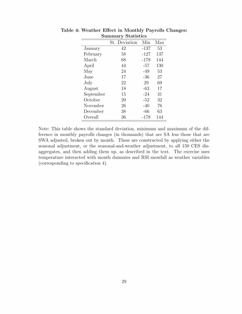
Table 4: Weather Effect in Monthly Payrolls Changes:Summary Statistics

St. Deviation Min MaxJanuary 42 -137 53February 58 -127 137March 68 -178 144April 44 -57 130May 24 -49 53June 17 -36 27July 22 29 69August 18 -63 17September 15 -24 31October 20 -52 32November 26 -40 76December 38 -66 63Overall 36 -178 144

Note: This table shows the standard deviation, minimum and maximum of the dif-ference in monthly payrolls changes (in thousands) that are SA less those that areSWA adjusted, broken out by month. These are constructed by applying either theseasonal adjustment, or the seasonal-and-weather adjustment, to all 150 CES dis-aggregates, and then adding them up, as described in the text. The exercise usestemperature interacted with month dummies and RSI snowfall as weather variables(corresponding to specification 4).

29

Table 5: Autocorrelation and Standard Deviation of Month-over-MonthChanges in SA and SWA Nonfarm Payrolls Data by Sector

Sector Autocorrelation Standard DeviationSA data SWA data SA data SWA data

Mining and logging 0.662 0.686 5.1 5.0Construction 0.586 0.768 39.0 35.9Manufacturing 0.739 0.756 50.4 50.2Trade, transportation and utilities 0.631 0.651 53.2 52.7Information 0.625 0.645 23.2 23.0Professional and business services 0.572 0.609 53.7 52.9Leisure and hospitality 0.324 0.374 28.6 27.2Other services 0.496 0.533 8.9 8.8Government 0.036 0.034 51.5 51.2Total 0.800 0.840 214.4 210.7

Note: This table reports the first order autocorrelation and standard deviation ofSA month-over-month payrolls changes (in thousands; total and by industry) and ofthe corresponding SWA data. The exercise uses temperature interacted with monthdummies and RSI snowfall as weather variables (corresponding to specification 4).

30

Table 6: Coefficient Estimates for Equation (3)

Real GDP C I G X Zγ1 0.08∗∗∗ 0.04∗∗ 0.19 0.06 0.26∗∗ 0.15∗

(0.03) (0.02) (0.12) (0.03) (0.11) (0.09)γ2 0.11∗∗ 0.06 0.29 -0.08 0.28 0.09

(0.05) (0.05) (0.28) (0.06) (0.18) (0.13)γ3 0.04 0.01 -0.33 0.07 0.08 -0.27

(0.04) (0.05) (0.37) (0.05) (0.23) (0.19)γ4 0.05 0.02 -0.09 0.07 0.12 -0.10

(0.04) (0.04) (0.22) (0.05) (0.14) (0.11)γ5 0.21 -0.06 7.29∗ -2.83∗∗ 0.68 -1.22

(0.80) (0.56) (4.16) (1.41) (2.90) (2.85)

Note: This table shows the coefficient estimates for the weather variables only whenestimating equation (3) for real GDP growth and five components thereof. Standarderrors are included in parentheses. The sample period is 1990Q1-2015Q2 (August2015 vintage data). Data units are as follows—NIPA growth rates: annualized per-centage points, temperature: degrees C, snowfall: mm. The columns labeled C, I, G,X and Z refer to personal consumption, private investment, government expenditures,export and imports, respectively.

31

Table 7: Adjustments to NIPA variable growth rates in 2015

SA data SWA data SSWA dataReal GDP 2015 Q1 0.6 1.4 3.2

2015 Q2 3.7 2.8 2.4C 2015 Q1 1.7 2.0 2.3

2015 Q2 3.1 2.7 3.0I 2015 Q1 8.6 9.6 12.7

2015 Q2 5.2 3.2 1.2G 2015 Q1 -0.1 0.6 0.9

2015 Q2 2.6 2.4 1.3X 2015 Q1 -6.0 -3.6 2.2

2015 Q2 5.2 3.1 1.0Z 2015 Q1 7.1 8.4 8.4

2015 Q2 2.8 2.0 1.5

Note: This table shows the quarter-over-quarter growth rates of real GDP and fivecomponents thereof in 2015Q1 and 2015 Q2. All entries are in annualized percentagepoints. The column labeled SA data refers to the published seasonally adjusted data.The column labeled SWA data refers to applying the weather adjustment describedin section 4 to the seasonally adjusted series. The column labeled SSWA data refersto applying another round of seasonal adjustment to the SWA series, using the X-13default settings. The rows labeled C, I, G, X and Z refer to personal consumption,private investment, government expenditures, export and imports, respectively.

32

Figure 1: Estimated MIDAS Polynomial

0 5 10 15 20 25 300

0.05

0.1

0.15

0.2

Wei

ght

j

Specification 4

0 10 20 30 40 50 60 70 80 90-0.02

0

0.02

0.04

0.06

0.08

0.1

Wei

ght

j

Specification 7

Note: This plots the weights wj against j (in days) where parameters are set equal to their maximumlikelihood estimates, fitting equation (1) to aggregate NSA employment, in specifications 4 and 7. Theweight for j = 0 is the weight attributed to unsual weather on the 12th day of the month (correspondingto the CES survey date).

33

Figure 2: Difference between SA and SWA Month-over-Month PayrollsChanges

Jan90 Jan95 Jan00 Jan05 Jan10 Jan15

-500

0

500

Em

ploy

men

t (0

00s)

SA and SWA Month-over-Month Payrolls Changes

SASWA

Jan90 Jan95 Jan00 Jan05 Jan10 Jan15-200

-100

0

100

200

Em

ploy

men

t (0

00s)

SA less SWA Month-over-Month Payrolls Changes

Note: This shows the month-over-month change in total nonfarm payrolls using standard seasonaladjustment less the corresponding change using seasonal-and-weather adjustment. This shows the es-timated effect of the weather, including the effect of controlling for the weather on seasonal factors.The exercise uses temperature interacted with month dummies and RSI snowfall as weather variables(corresponding to specification 4).

34

Figure 3: Autocorrelation of Weather Effects

5 10 15 20

−0.5

−0.4

−0.3

−0.2

−0.1

0

0.1

0.2

0.3

0.4

0.5

Lag (months)

Note: This shows the sample autocorrelation function of weather effects, defined as the month-over-month change in total nonfarm payrolls using standard seasonal adjustment less the corresponding changeusing seasonal-and-weather adjustment. The horizontal dashed lines are the critical values for sampleautocorrelations to be statistically significant at the 5 percent level. The exercise uses temperatureinteracted with month dummies and RSI snowfall as weather variables (corresponding to specification4).

35

Figure 4: Difference between SA and SWA Month-over-Month PayrollsChanges in Construction

Jan90 Jan00 Jan10-60

-40

-20

0

20

40

60

Em

ploy

men

t (0

00s)

Note: This shows the month-over-month change in construction payrolls using standard seasonal adjust-ment less the corresponding change using seasonal-and-weather adjustment. This shows the estimatedeffect of the weather, including the effect of controlling for the weather on seasonal factors. The exerciseuses temperature interacted with month dummies and RSI snowfall as weather variables (correspondingto specification 4).

36

Figure 5: Difference between SA and SWA Month-over-Month PayrollsChanges: Using Specification 5

Jan90 Jan00 Jan10

-200

-150

-100

-50

0

50

100

150

200

Em

ploy

men

t (0

00s)

Note: As for Figure 2, except that CPS work absences due to weather is added as an additional weathervariable (as in specification 5).

37

Figure 6: Difference between SA and SWA Month-over-Month PayrollsChanges: Using Specification 6

Jan90 Jan00 Jan10

-200

-150

-100

-50

0

50

100

150

200

Em

ploy

men

t (0

00s)

Note: As for Figure 2, except that lags of weather indicators in the previous two months are included(as in specification 7).

38