wear estimation in flexible multibody systems · pdf filewear estimation in flexible multibody...

MULTIBODY DYNAMICS 2005, ECCOMAS Thematic ConferenceJ.M. Goicolea, J. Cuadrado, J.C. Garcıa Orden (eds.)

Madrid, Spain, 21–24 June 2005

WEAR ESTIMATION IN FLEXIBLE MULTIBODY SYSTEMS WITHAPPLICATION TO RAILROADS

Thomas B. Meinders?, Peter Meinke? and Werner O. Schiehlen?

?Institute B of Mechanics, University of Stuttgart, Germanye-mail: [email protected]

web page:http://www.mechb.uni-stuttgart.de/staff/Schiehlen

Keywords: Flexible multibody systems, wear estimation, railroads

Abstract. The main focus of this paper is the investigation of the wear process of flexiblewheelsets modelled as flexible multibody systems. The wear model is based on the mass losscaused by the contact forces between wheel and rail and the slip values in the contact patch. Thewear model developed is used together with a modul for the wheel-rail contact and considersthe amount of mass loss which is proportional to the frictional power which follows from contactforce acting along the slip direction. Torque and slip of the twisting motion are not consideredin the computation of the frictional power. The wear reduces the radius uniformly over theprofile width, it does not change the wheel profile. In addition, the wear model is extended tolong-term phenomena of the wear. For this purpose a feedback loop is introduced resultingin the development of wheel polygons. The changing wheel radius is fed back to the contactmodule.

Results are presented for the dynamics and the wear of elastic wheelsets. Due to the highspeeds of recent intercity trains, the rotor dynamics of the wheelset is considered. The weardevelopment due to initial out-of-roundness of the wheels is investigated.

1

[email protected]

http://www.mechb.uni-stuttgart.de/staff/Schiehlen

Thomas B. Meinders, Peter Meinke and Werner O. Schiehlen

1 INTRODUCTION

High speed trains like the Intercity Express (ICE) in Germany (1991) may lead to new andpoorly understood problems following from their speed. One major problem was easily noticedby passengers due to a loud and disturbing droning noise. The responsible structural vibrationsof the car body were excited by out-of-round wheels, which obviously lost their original roundshape under the influence of irregular wear. Consequently, the changing wheel shape werecausing accelerated wear such that the wheels had to be reprofiled after reaching a critical limit.The characteristic frequency for the excited vibrations of the car body was in the range of70–100 Hz, which is in the so-called medium frequency range (30–300 Hz).

In order to analyse the rotor dynamics and possible mechanisms for the wear development, anappropriate approach to model flexible bodies in the medium-frequency range has to be selected.Combining the advantages of rigid multibody systems and finite element systems a suitablemethod is available to account for the first eigenmodes of the wheelset in the questionablefrequency range.

2 FLEXIBLE MULTIBODY SYSTEMS

The method of multibody systems using a minimum set of generalized coordinates hasproven to be a very suitable and successful method for the analysis of constrained mechani-cal systems, as shown by Schiehlen [21]. In addition to the rigid body approach, where rigidbodies can be connected through massless joints and force elements the extension towards flexi-ble bodies enables the consideration of structural deflections of selected bodies of the multibodysystem.

The approach to model flexible multibody systems used in this paper is based on the ideaassuming large gross motions and superimposed small flexible deformations. For the discretiza-tion of the elastic body either local or global shape functions can be used. Due to the flexibilityto model even very complex geometric structures, local shape functions (finite element method)have been chosen. The deformation of the structure is described by the modal approach, i.e.through space dependent mode shapes and time dependent modal coordinates, as presentedby Shabana [22]. The flexible body approach is widely used in vehicle dynamics, see e.g.Ambrosio and Goncalves [1], Claus and Schiehlen [2], and Meinders and Meinke [13].

2.1 Kinematics and Dynamics

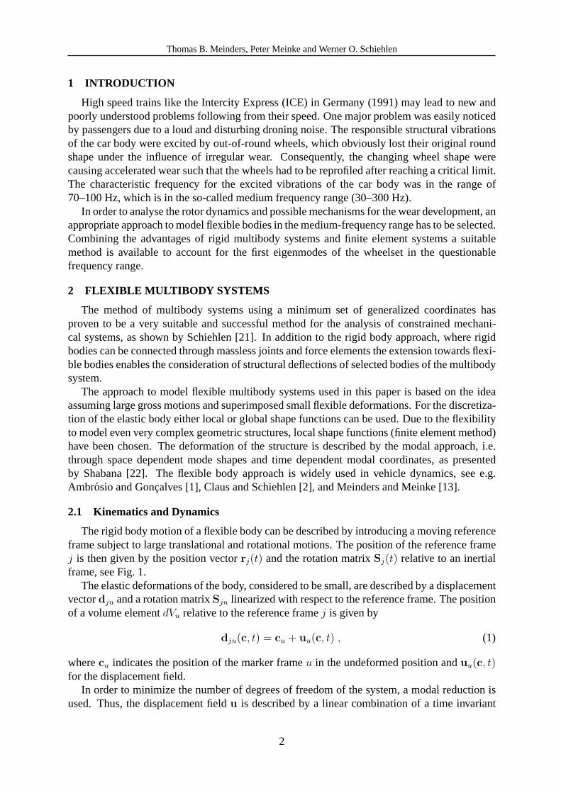
The rigid body motion of a flexible body can be described by introducing a moving referenceframe subject to large translational and rotational motions. The position of the reference framej is then given by the position vectorrj(t) and the rotation matrixSj(t) relative to an inertialframe, see Fig.1.

The elastic deformations of the body, considered to be small, are described by a displacementvectordju and a rotation matrixSju linearized with respect to the reference frame. The positionof a volume elementdVu relative to the reference framej is given by

dju(c, t) = cu + uu(c, t) , (1)

wherecu indicates the position of the marker frameu in the undeformed position anduu(c, t)for the displacement field.

In order to minimize the number of degrees of freedom of the system, a modal reduction isused. Thus, the displacement fieldu is described by a linear combination of a time invariant

2


r j(t) Sj(t)

dju

cuuu

dVu

r S

Sj (t0)r j(t0)

Sju

cu

dVu

Figure 1:Definition of deformation and reference vector.

translational mode shape matrixΦ, containing selected deformation modes, and the vectorq ofgeneralized elastic coordinates, which are functions of time only:

uu(c, t) = Φ(c)q(t) . (2)

Assuming only small deformations, the rotation matrixSju, accounting for the orientation ofthe marker frameu relative to the reference framej, is accordingly described as

Sju(c, t) = I + ϑ(c, t) , (3)

whereI denotes a [3x3] identity matrix andϑ a skew-symmetric matrix due to the rotationalelastic deformations. The matrixϑ is derived from the vector of small rotationsϑ = [α β γ]T .According to (2) this rotation vector can be expressed as a linear combination of a time-invariantmode shape matrixΨ and the vectorq of generalized elastic coordinates

ϑu(c, t) = Ψ(c)q(t) . (4)

As mentioned before the discretization of the elastic body can be accomplished either byusing local or global shape functions. The advantage of local shape functions is, that evencomplex geometric structures can be described. Thus using the finite element method, thetranslational mode shape matrix (2) can be expressed by

Φ(c) = STA(c) SBT , (5)

whereA(c) is the element shape function matrix,B is the Boolean matrix describing the as-semblage of the finite elements andT denotes the modal matrix, summarizing the mode shapesof the structure. The matricesS and S transform the displacements from the element to thereference frame. The rotational mode shape matrixΨ is obtained in a completely analoguemanner.

3


Before deriving the equations of motions the absolute position and orientation as well as theabsolute velocities and accelerations of the marker frameu attached to the volume elementdVu

of the elastic body have to be formulated:

ru = rj + dju = rj + (cu + uu) ,

Su = SjSju . (6)

The expressions for the absolute velocities and accelerations can be derived using relativekinematics, see Melzer [15]. Applying D’Alembert’s principle the equations of motion of aflexible multibody system can be written as

M(y, t) y(t) + kc(y, y, t) + ki(y, y) = qf (y, y, t) , (7)

with the mass matrixM, the vector of generalized gyroscopic forceskc, the vector of stiffnessand damping forceski, and the vector of generalized applied forcesqf . The generalized coor-dinates of the system are assembled in the vectory, with the vector of the rigid body motionyr

and the vector of elastic coordinatesq as sub-vectors, such that

y(t) = [yr(t) q(t)]T . (8)

Various volume integrals have to be evaluated to obtain the mass matrix. Since small de-formations are assumed, these volume integrals can be expanded into a Taylor series of elasticcoordinates up to first order. The coefficient matrices of the Taylor series, the so-called shapeintegrals, are calculated by numerical integration. Since the shape integrals are independent oftime, they can be computed prior to time integration by pre-processing. A detailed descriptionof this approach can be found in Melzer [15] and Piram [17].

3 MODELING OF ROTATING WHEELSETS

The first step in creating a simulation tool to investigate the development of out-of-roundwheels is to set up an appropriate mechanical model of the wheelset. The essential stepsto model the wheelset type BA 14 of the Deutsche Bahn AG, which is the commonly-usedwheelset for the German high-speed train ICE 1, are described in the following subsections.

3.1 Finite Element Model of the Wheelset

The symmetry of the wheelset equipped with altogether 4 disk-brakes is used for the de-scription of the discretized structure by the finite element software ANSYS [18]. In order togain a maximum of flexibility, the geometric shape of the wheelset is characterized by a set of54 geometric parameters, as described by Meinders [10]. The 3D finite element structure isgenerated by rotating a 2D mesh of the wheelset as explained by Meinders [11]. The elementsused in this model are SOLID73 from the ANSYS library which provide 6 degrees of freedomfor each of the 8 nodes. This is an important requirement for the later use of the finite elementdata in the flexible multibody system.

The connection between the finite element model of the wheelset and the description of therigid body model (springs, dampers, bogie coach, rail, etc.) is achieved by a limited number ofso-called marker framesu, as shown in Fig.1. The information about the flexible properties ofthe body in terms of shape integral matrices is only provided for these selected marker nodes ofthe finite element model. The reason for this reduction is to keep the size of the overall modeland thus the computation time in reasonable limits.

4


In case of a rotating wheelset the rotation itself is described by a reference frame which islocated in the middle of the wheelset on its centerline. Therefore, each node of the structurethat is not located on the centerline will rotate with the reference frame with respect to theinertial frame. This can be easily avoided for the interconnecting marker nodes of the primarysuspension as well as the marker nodes later needed for the modeling of unbalances by choosingnodes lying directly on the centerline.

The essential wheel-rail contact of the wheelset with its forces and moments is acting on thewheel surface. Therefore, it is not feasible to select one specific node from the surface of thewheels finite element structure since those nodes are rotating relative to the inertial frame.

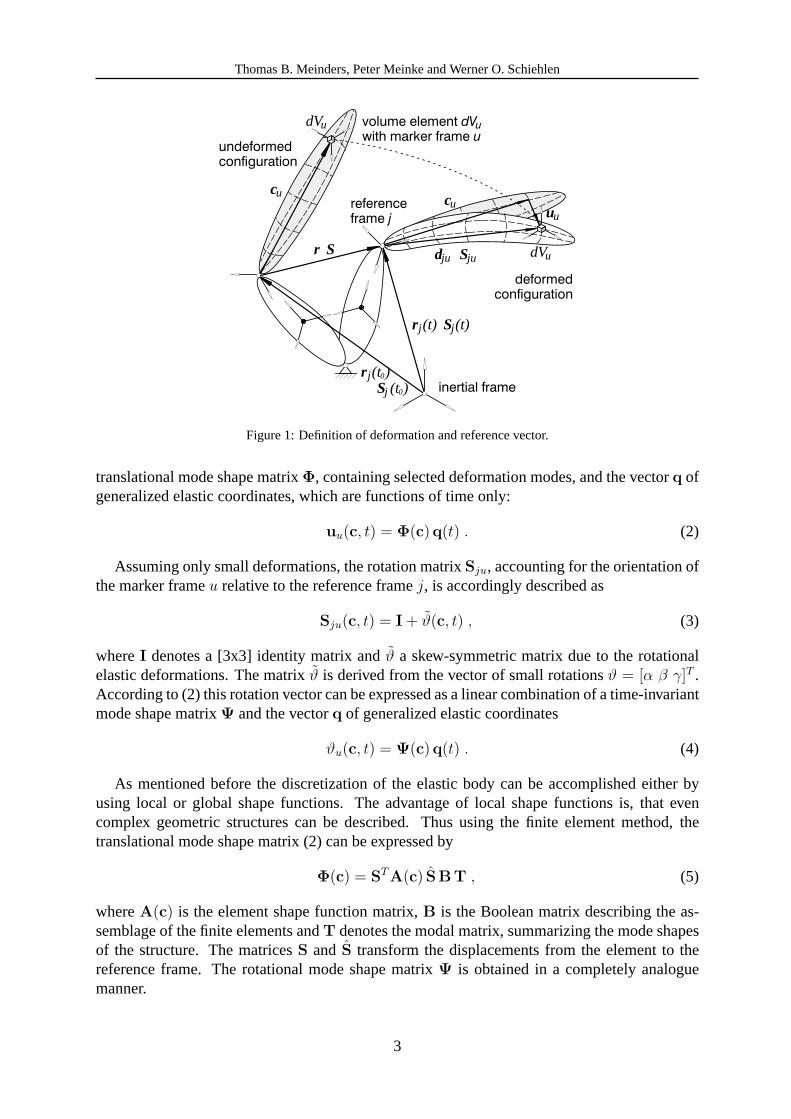
The modeling challenge to realize a non-rotating wheel-rail force acting on the surface of thewheel can be resolved using the following important property of the wheelset: The eigenmodeanalysis of the FE-structure for the unsupported wheelset (see Fig.2) as well as for the sup-ported case showed that the wheel-rim has no significant deformation in the frequency rangeof 0–300 Hz. Thus, the wheel-rim can be treated as a rigid body for the investigation in themedium frequency range.

Using this property of the wheel the degrees of freedom of the wheel-rim elements are con-strained and supplemented by four also constrained beam elements such that the motion of therim is represented by the center-point in the middle of the wheel, as shown in Fig.3. Thiscenter-point is subsequently chosen as a marker node. Thus, the necessary wheel-rail contactforces and moments can act on the wheel-rim even though they are applied to the marker in themiddle of the wheel.

3.2 Modal Analysis and Selection of the Elastic Coordinates

The first step in analysing and understanding the dynamical properties of the wheelset is amodal analysis. Subsequently the knowledge about the eigenbehaviour in the medium-frequencyrange is used to select the eigenmodes needed as elastic coordinates in the flexible multibodysystem.

The resulting eigenmodes of the unsupported wheelset in the frequency range up to 290 Hzare presented in Fig.2. At a frequency of 82,5 Hz the first elastic eigenmode of the wheelsetis characterized by a torsional motion of one side of the wheelset against the other with a nodalpoint between the two inner disk-brakes (1st anti-metric torsional mode). The next two eigen-frequencies at 84,6 Hz are the1st symmetric bending mode in vertical and horizontal direction.At this low frequency wheels and disk-brakes obviously still behave as if they were rigid. Thisis not true any more for the1st anti-metric bending mode at 131,8 Hz. At this frequency theflexibility of the wheel membrane influences the movement of the wheels. This can also befound for the2nd symmetric bending mode at 188,5 Hz, where wheels and disk-brakes bendin opposite directions. At a frequency of 235 Hz the wheel-rims are moving symmetricallyalong the wheelsets axis. This eigenmode is therefore called1st symmetric umbrella mode.The1st symmetric torsional mode at 261 Hz has four nodal points, where the wheels and innerdisk-brakes are moving in the same orientation. The last eigenmode in the frequency range upto 300 Hz is the1st anti-metric umbrella mode at 296,1 Hz.

Based on the knowledge of the eigenbehaviour of the wheelset an accurate selection of typeand number of the eigenmodes taken into account for the inclusions in the flexible multibodysystem is required. Several simulations with different sets of eigenmodes have shown that theumbrella modes as well as the1st symmetric torsional mode are not necessary to describe thestructural vibrations of the wheelset based on the given boundary-conditions and excitationsthrough unbalances, out-of-round wheels or rail imperfections. As a consequence the following

5


1st anti–metric torsional mode (82,5 Hz)

1st symmetric bending mode (84,6 Hz)

1st anti–metric bending mode (131,8 Hz)

2nd symmetric bending mode (188,5 Hz)

1st symmetric umbrella mode (235 Hz)

1st symmetric torsional mode (261 Hz)

Figure 2:Eigenmodes of an unsupported wheelset in the frequency range up to 290 Hz

Figure 3:Center-point

6


$## # ! !$" !#) #!(

$## " !" $"" !" #!("#"!#

!"!# "#$## #

(

(

!'# #&" %

#!# ## !"

#!# ## #! #

#!"!#

#!#

"# ## #

## !

"#!$# ! "#!"""

!#

Figure 4:Modular organization of the contact module

seven eigenmodes are included in the model as generalized elastic coordinates:

• 1st anti-metric torsional mode

• 1st symmetric bending mode (vertical & horizontal)

• 1st anti-metric bending mode (vertical & horizontal)

• 2nd symmetric bending mode (vertical & horizontal)

4 WHEEL-RAIL CONTACT MODULE

Railway dynamics are highly influenced by the complex wheel-rail contact situation. Espe-cially for the investigation of wear happening between wheel and rail, a detailed model of thiscomplex contact geometry is essential.

One such detailed model is the wheel-rail contact module of Kik and Steinborn [4], whichwas originally developed for the use in the multibody system software MEDYNA. Due to itswell-defined input-output structure it was possible to extend the multibody system softwareNEWEUL/NEWSIM [7] with the ability to describe complex railway systems. A detailed reportabout the integration of the wheel-rail contact module as a force element in the software packageNEWEUL/NEWSIM is given by Volle [24].

4.1 Modular Approach of the Contact Module

The principal modular structure of the contact module is shown in Fig.4. Based on thecurrent position of the wheelj relative to the rail-headi the position vectorra and the rotationvectorγa as well as the relative velocitiesva and angular velocitiesωa serve as the fundamental

7


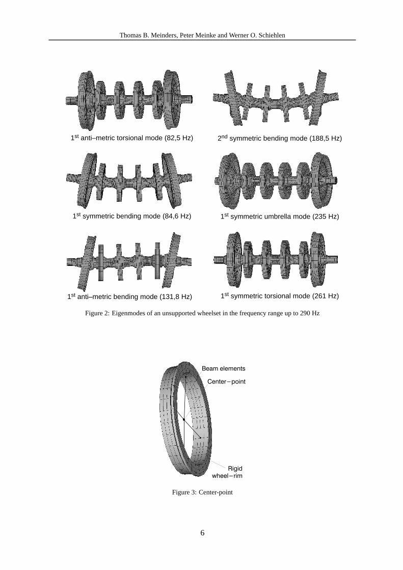
Figure 5:Definition of wheel profile and wheel radius

input parameters for the wheel-rail contact module. Needed for each step of the numerical timeintegration of the system, the contact module provides the contact forcesFwr and momentsMwr

acting between wheel and rail.As shown in Fig.4 the contact module is split up into three parts that need to be completed

in order to obtain all data for the given contact situation:The contact module enables the use of different spline approximated profiles for wheel and

rail. The profiles used for the simulations presented in this paper are UIC60 and S1002. Basedon the given relative position of the wheel relative to the rail the 3D contact geometry is trans-formed into a 2D plane as shown in Fig.4. Consequently the contact zones and contact pointscan be determined. Finally the information obtained from this 2D contact situation is trans-formed back onto the 3D bodies of wheel and rail. The output data obtained from the geometricpart of the contact module are essentially the number and position of the contact points, theresulting penetrations in the contact points and the angles of contact.

The second part of the contact module, the normal contact part, uses the values of the half-axes of the ellipses and the penetration to compute the normal forces based on Hertzian Theory.

Finally the tangential contact part of the module computes the tangential forces, twistingmoments as well as the slip values. The contact theory used in this part of the model is Kalker’ssimplified theory, also often referred to as the FASTSIM algorithm.

4.2 Varying Wheel Radii During Time Integration

One important requirement for the use of the wheel-rail contact module is the possibility todescribe varying wheel radii depending on the present angular position of the wheel. Since thefocus of the wear investigation requires these radii to change over time the radiusrj(ϕ) has yetto be another input value to the contact module.

As depicted in Fig.5 the local coordinate system for the definition of the wheel profileCj isnot laying in the middle of the wheel, but in the wheels profile itself. By changing the size ofthe radiusrj(ϕ) the wheels profile in its locally defined coordinate systemCj is changed as awhole.

4.3 Track Model

The track as part of the contact module is a flexible system, too. In this section the trackmodel is shortly reviewed. A more detailed description is given in Meinders [14].

For the modeling of the track dynamics in the medium frequency range, a modal approach isused. The basic idea of that approach is to represent the dynamics of the system by superposition

8


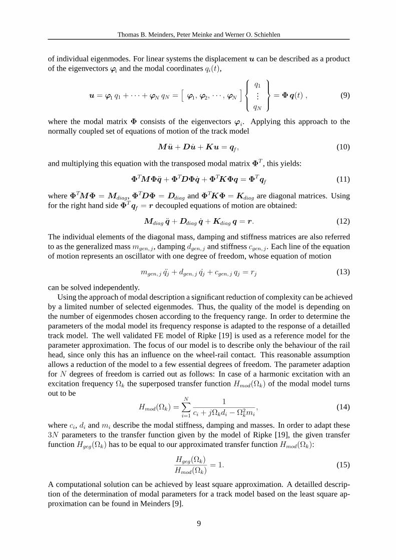
of individual eigenmodes. For linear systems the displacementu can be described as a productof the eigenvectorsϕi and the modal coordinatesqi(t),

u = ϕ1 q1 + · · ·+ ϕN qN =[

ϕ1, ϕ2, · · · , ϕN

]

q1...

qN

= Φ q(t) , (9)

where the modal matrixΦ consists of the eigenvectorsϕi. Applying this approach to thenormally coupled set of equations of motion of the track model

Mu + Du + Ku = qf , (10)

and multiplying this equation with the transposed modal matrixΦT , this yields:

ΦTMΦq + ΦTDΦq + ΦTKΦq = ΦT qf (11)

whereΦTMΦ = Mdiag, ΦTDΦ = Ddiag andΦTKΦ = Kdiag are diagonal matrices. Usingfor the right hand sideΦT qf = r decoupled equations of motion are obtained:

Mdiag q + Ddiag q + Kdiag q = r. (12)

The individual elements of the diagonal mass, damping and stiffness matrices are also referredto as the generalized massmgen, j, dampingdgen, j and stiffnesscgen, j. Each line of the equationof motion represents an oscillator with one degree of freedom, whose equation of motion

mgen, j qj + dgen, j qj + cgen, j qj = rj (13)

can be solved independently.Using the approach of modal description a significant reduction of complexity can be achieved

by a limited number of selected eigenmodes. Thus, the quality of the model is depending onthe number of eigenmodes chosen according to the frequency range. In order to determine theparameters of the modal model its frequency response is adapted to the response of a detailledtrack model. The well validated FE model of Ripke [19] is used as a reference model for theparameter approximation. The focus of our model is to describe only the behaviour of the railhead, since only this has an influence on the wheel-rail contact. This reasonable assumptionallows a reduction of the model to a few essential degrees of freedom. The parameter adaptionfor N degrees of freedom is carried out as follows: In case of a harmonic excitation with anexcitation frequencyΩk the superposed transfer functionHmod(Ωk) of the modal model turnsout to be

Hmod(Ωk) =N∑

i=1

1

ci + jΩkdi − Ω2kmi

, (14)

whereci, di andmi describe the modal stiffness, damping and masses. In order to adapt these3N parameters to the transfer function given by the model of Ripke [19], the given transferfunctionHgeg(Ωk) has to be equal to our approximated transfer functionHmod(Ωk):

Hgeg(Ωk)

Hmod(Ωk)= 1. (15)

A computational solution can be achieved by least square approximation. A detailled descrip-tion of the determination of modal parameters for a track model based on the least square ap-proximation can be found in Meinders [9].

9


For the simulation of railroad vehicles it is essential to describe the dynamic behaviour of thetrack regardless whether an excitation happens to be over the sleeper of the track or in between.Thus, the parameters of the modal model are determined for two characteristic positions, that isexactly over the sleeper and in the middle of the sleeper bay. The continuous desciption of thetrack dynamics in the medium frequency range can be achieved by a periodic distribution of themodal parameters as proposed by Fingberg and Popp [3]:

pi(l) =psi + pmi

2+

psi − pmi

2

cos

(2πl

L

)+

1− cos(

4πlL

)

4

. (16)

Thereinpsi (index s for sleeper) andpmi (index m for middle) describe the modal parametersover the sleeper and in the sleeper bay. The position between to sleepers is given by the variablelwith L accounting for the total length of the sleeper bay.

The correlation between the original frequency response and the response of the approxi-mated modal model is depending on the number of degrees of freedom for the modal model.This number should be chosen according to the number of response peaks in the desired fre-quency range. As for the vertical dynamics of the track between 0–500 Hz there are two re-sponse peaks found in that frequency range.

4.4 Dynamical analysis fo the vehicle system

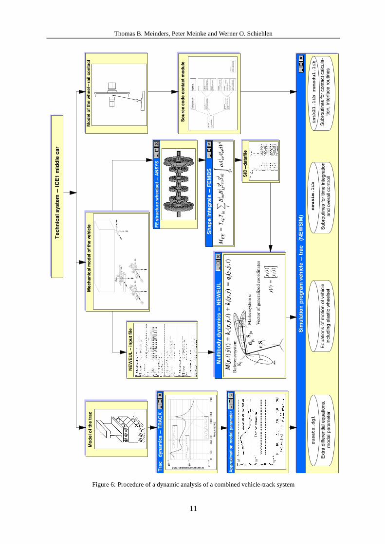
With models of the wheelset, the wheel-rail contact and the track presented, the procedureof the dynamic analysis of such a flexible system is shown in Fig.6.

Starting from the real engineering system of an ICE1 middle car, it is divided into the threemechanical models: track, vehicle and wheel-rail contact. As shown on the left of Fig.6the model of the track is described through the computational code TRACK developed byRipke [20]. In order to get a good respresentation of the dynamical behaviour of the track inthe medium frequency range between 30–300 Hz, the parameters of a modal model are adaptedto the computed frequency response of TRACK. The resulting parameters together with thecorresponding differential equations are one component of the overall simulation program.

The generation of the equations of motion of the vehicle and flexible wheelset is shownin the middle of Fig.6. The flexible wheelset is discretized using a finite element software,e.g. ANSYS [18]. The resulting data for the mass and stiffness matrix as well as the user-selected eigenmodes of the elastic body is used in a preprocessor, e.g. FEMBS [25], in orderto compute the shape integrals describing the elastodynamical behaviour. To gain a maximumof software interoperability, these terms are saved in a standardized format (SID) describedby Wallrapp [26]. The equations of motion can be computed by a multibody system code,e.g. NEWEUL [7]. Reading the input-file defining the topological structure of the multibodysystem and the SID-file containing the information about the elastic body, NEWEUL yieldsmixed symbolic-numerical equations of motion. Those are written as files in FORTRAN syntax,they will be later integrated as source code into the overall simulation program.

The description and computational realization of the wheel-rail contact is accomplished us-ing the software code of Kik [4] (right part of Fig.6). The modul is provided to the simula-tion program as a libraryintk21.lib . The appropriate communication between the contactmodul and the simulation subroutines in the libarynewsim.lib is realized via an interfacersmodul.lib developed by Volle [24].

Finally all files are compiled and linked together with the libraries as described in Fig.6.The resulting problem specific simulation program of the vehicle-wheelset-track system can be

10


% #(&!'

NE

WE

UL

– in

pu

t fi

le

)!($- -#"'

#! "$! $ ( *!

(!

"

)!($# %&$&" *!

(&

'(&)()& +!'(

& -#"'

$! $ ( (&

$! $ ( +!&! $#((

%%&$,"

($# "

$! %&"(&

newsim.lib

intk21.lib rsmodul.lib

zusatz.dgl

#! '-'("

"

! &

$)& $ $#(( "$)!

Figure 6:Procedure of a dynamic analysis of a combined vehicle-track system

11


used to analyse the dynamics of the total system.

5 LONG-TERM WEAR MODEL

The main focus of this paper is the investigation of the wear process of the wheelset. Oneaspect of this is to determine the amount of mass loss caused by the contact forces and slipvalues. In order to describe this complex wear process, quite a number of different wear modelshave been developed, see Kim [5], Specht [23] and Zobory [27]. The wear hypotheses andmodel for the mass loss used in this paper is presented in Sect.5.1.

The second part of the wear model is dealing with the long-term effects of the wear. Itis therefore necessary to introduce a feedback loop, such that the changing wheel profile isinfluencing the contact situation between wheel and rail. This influence, often also referred toas long-term behaviour, is happening on a very long time scale that is not accessible throughdirect time integration, as shown by Meinders and Meinke [13].

5.1 Wear Hypothesis and Model for the Mass Loss

The wear model developed for the use together with the contact module from Sect.4 is basedon the following assumptions, see Meinders [12] and Luschnitz [8]:

• The amount of mass loss is proportional to the frictional power (hypothesis of frictionalpower)

• The wear factork distinguishes between mild and severe wear

• The frictional power is determined through the contact forces acting in the direction ofslip

• Torque and slip of the twisting motion are not considered for the calculation of frictionalpower

• The wear reduces the radius uniformly over the profiles width. It does not change theform of the wheel profile

As mentioned above, the presented wear model is based on the hypothesis, that the loss ofmaterial∆m due to wear is basically proportional to the friction workWR

∆m = k WR . (17)

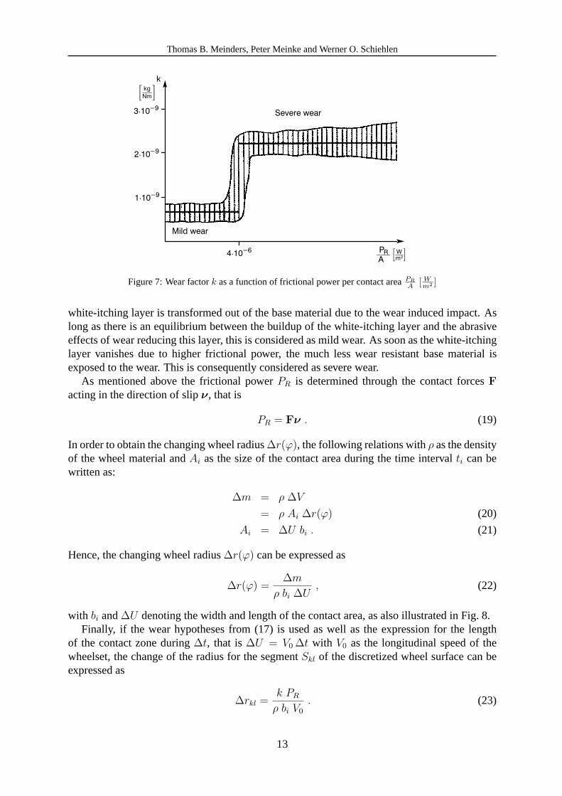
The proportional factork in (17) is not the same though for all values of frictional power. In factmeasurements described by Krause and Poll [6] have shown that the wear factork is suddenlyincreasing to a much higher value when a certain frictional power based on the contact area isreached. To reflect this characteristic also shown in Fig.7, the wear model is distinguishingbetween mild and severe wear using the following wear parameters:

k =

7 · 10−10 kg

Nm: PR

A≤ 4 · 10−6 W

m2 mild wear2.1 · 10−9 kg

Nm: PR

A> 4 · 10−6 W

m2 severe wear. (18)

The physical explanation for this sudden increase of the wear parameterk is also given byKrause and Poll [6]: The material surface of the wheels consists of a thin so-called white-itchinglayer, which shows a higher resistance against wear than the underlying base material. This

12


Figure 7:Wear factork as a function of frictional power per contact areaPR

A [ Wm2 ]

white-itching layer is transformed out of the base material due to the wear induced impact. Aslong as there is an equilibrium between the buildup of the white-itching layer and the abrasiveeffects of wear reducing this layer, this is considered as mild wear. As soon as the white-itchinglayer vanishes due to higher frictional power, the much less wear resistant base material isexposed to the wear. This is consequently considered as severe wear.

As mentioned above the frictional powerPR is determined through the contact forcesFacting in the direction of slipν, that is

PR = Fν . (19)

In order to obtain the changing wheel radius∆r(ϕ), the following relations withρ as the densityof the wheel material andAi as the size of the contact area during the time intervalti can bewritten as:

∆m = ρ ∆V

= ρ Ai ∆r(ϕ) (20)

Ai = ∆U bi . (21)

Hence, the changing wheel radius∆r(ϕ) can be expressed as

∆r(ϕ) =∆m

ρ bi ∆U, (22)

with bi and∆U denoting the width and length of the contact area, as also illustrated in Fig.8.Finally, if the wear hypotheses from (17) is used as well as the expression for the length

of the contact zone during∆t, that is∆U = V0 ∆t with V0 as the longitudinal speed of thewheelset, the change of the radius for the segmentSkl of the discretized wheel surface can beexpressed as

∆rkl =k PR

ρ bi V0

. (23)

13


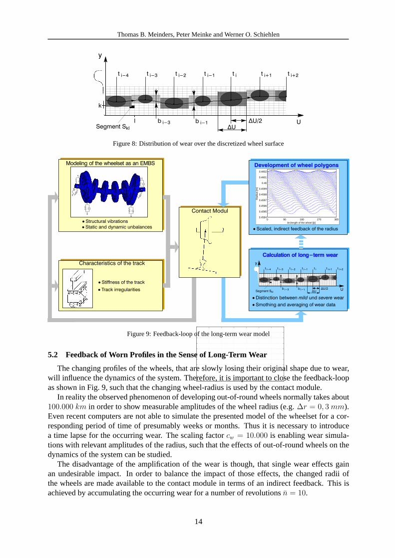
Figure 8:Distribution of wear over the discretized wheel surface

"" #

" %!" !

" !"! " "

" #"# $ "!

"" & #!

"!! " "

# "!

!"" "% # %

" $ % "

" " #!

&

" " " " " " "

"

1 2 3 4 5 6 70

0.5

1

1.5

2

2.5

3

3.5

4

4.5

5x 10

−7

Order of polygonalisation

0 90 180 270 3600.4594

0.4595

0.4596

0.4597

0.4598

0.4599

0.46

0.4601

0.4602

Arclength of the wheel [ϕ]

Radiu

s [m

]

Figure 9:Feedback-loop of the long-term wear model

5.2 Feedback of Worn Profiles in the Sense of Long-Term Wear

The changing profiles of the wheels, that are slowly losing their original shape due to wear,will influence the dynamics of the system. Therefore, it is important to close the feedback-loopas shown in Fig.9, such that the changing wheel-radius is used by the contact module.

In reality the observed phenomenon of developing out-of-round wheels normally takes about100.000 km in order to show measurable amplitudes of the wheel radius (e.g.∆r = 0, 3 mm).Even recent computers are not able to simulate the presented model of the wheelset for a cor-responding period of time of presumably weeks or months. Thus it is necessary to introducea time lapse for the occurring wear. The scaling factorcw = 10.000 is enabling wear simula-tions with relevant amplitudes of the radius, such that the effects of out-of-round wheels on thedynamics of the system can be studied.

The disadvantage of the amplification of the wear is though, that single wear effects gainan undesirable impact. In order to balance the impact of those effects, the changed radii ofthe wheels are made available to the contact module in terms of an indirect feedback. This isachieved by accumulating the occurring wear for a number of revolutionsn = 10.

14


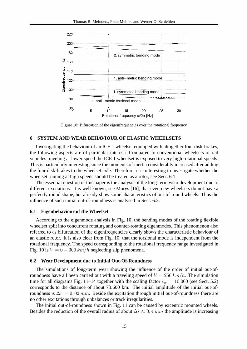
Figure 10:Bifurcation of the eigenfrequencies over the rotational frequency

6 SYSTEM AND WEAR BEHAVIOUR OF ELASTIC WHEELSETS

Investigating the behaviour of an ICE 1 wheelset equipped with altogether four disk-brakes,the following aspects are of particular interest: Compared to conventional wheelsets of railvehicles traveling at lower speed the ICE 1 wheelset is exposed to very high rotational speeds.This is particularly interesting since the moments of inertia considerably increased after addingthe four disk-brakes to the wheelset axle. Therefore, it is interesting to investigate whether thewheelset running at high speeds should be treated as a rotor, see Sect.6.1.

The essential question of this paper is the analysis of the long-term wear development due todifferent excitations. It is well known, see Morys [16], that even new wheelsets do not have aperfectly round shape, but already show some characteristics of out-of-round wheels. Thus theinfluence of such initial out-of-roundness is analysed in Sect.6.2.

6.1 Eigenbehaviour of the Wheelset

According to the eigenmode analysis in Fig.10, the bending modes of the rotating flexiblewheelset split into concurrent rotating and counter-rotating eigenmodes. This phenomenon alsoreferred to as bifurcation of the eigenfrequencies clearly shows the characteristic behaviour ofan elastic rotor. It is also clear from Fig.10, that the torsional mode is independent from therotational frequency. The speed corresponding to the rotational frequency range investigated inFig. 10 is V = 0− 300 km/h neglecting slip phenomena.

6.2 Wear Development due to Initial Out-Of-Roundness

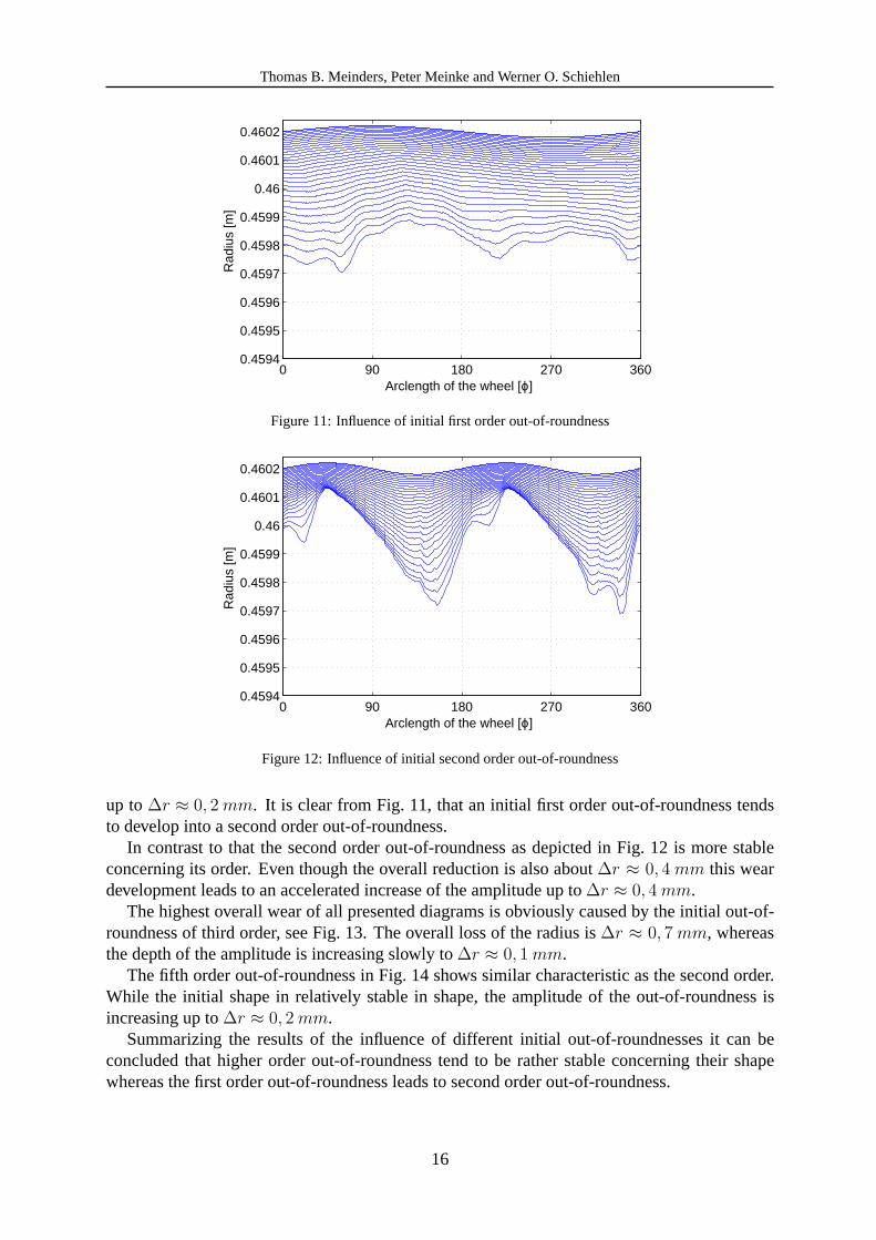
The simulations of long-term wear showing the influence of the order of initial out-of-roundness have all been carried out with a traveling speed ofV = 256 km/h. The simulationtime for all diagrams Fig.11–14 together with the scaling factorcw = 10.000 (see Sect.5.2)corresponds to the distance of about 73.600 km. The initial amplitude of the initial out-of-roundness is∆r = 0, 02 mm. Beside the excitation through initial out-of-roundness there areno other excitations through unbalances or track irregularities.

The initial out-of-roundness shown in Fig.11 can be caused by excentric mounted wheels.Besides the reduction of the overall radius of about∆r ≈ 0, 4 mm the amplitude is increasing

15


0 90 180 270 3600.4594

0.4595

0.4596

0.4597

0.4598

0.4599

0.46

0.4601

0.4602


Rad

ius

[m]

Figure 11:Influence of initial first order out-of-roundness

0 90 180 270 3600.4594

0.4595

0.4596

0.4597

0.4598

0.4599

0.46

0.4601

0.4602


Rad

ius

[m]

Figure 12:Influence of initial second order out-of-roundness

up to∆r ≈ 0, 2 mm. It is clear from Fig.11, that an initial first order out-of-roundness tendsto develop into a second order out-of-roundness.

In contrast to that the second order out-of-roundness as depicted in Fig.12 is more stableconcerning its order. Even though the overall reduction is also about∆r ≈ 0, 4 mm this weardevelopment leads to an accelerated increase of the amplitude up to∆r ≈ 0, 4 mm.

The highest overall wear of all presented diagrams is obviously caused by the initial out-of-roundness of third order, see Fig.13. The overall loss of the radius is∆r ≈ 0, 7 mm, whereasthe depth of the amplitude is increasing slowly to∆r ≈ 0, 1 mm.

The fifth order out-of-roundness in Fig.14 shows similar characteristic as the second order.While the initial shape in relatively stable in shape, the amplitude of the out-of-roundness isincreasing up to∆r ≈ 0, 2 mm.

Summarizing the results of the influence of different initial out-of-roundnesses it can beconcluded that higher order out-of-roundness tend to be rather stable concerning their shapewhereas the first order out-of-roundness leads to second order out-of-roundness.

16


0 90 180 270 3600.4594

0.4595

0.4596

0.4597

0.4598

0.4599

0.46

0.4601

0.4602


Radiu

s [m

]

Figure 13:Influence of initial third order out-of-roundness

0 90 180 270 3600.4594

0.4595

0.4596

0.4597

0.4598

0.4599

0.46

0.4601

0.4602


Rad

ius

[m]

Figure 14:Influence of initial fifth order out-of-roundness

17


7 SUMMARY

The approach of flexible multibody systems is used to analyse the rotor dynamics and thedeveloping irregular wear of elastic railway wheelsets. The modeling challenge of a rotatingflexible body exposed to the wheel-rail forces is resolved by applying the contact forces toa center-point, which is coupled to the wheel-rim through constrained equations. A modularwheel-rail contact module is integrated in the multibody system software NEWEUL/NEWSIM.In order to account for the appearing wear of the wheels a long-term wear model with a feedbackloop for the changing profiles is presented.

According to the eigenmode analysis which results in seven different eigenmodes of thewheelset in the medium frequency range up to 300 Hz, it is essential to consider the possibledeformations of the wheelset. The influence of the rotational speed on the bending eigenfre-quencies of the wheelset emphasize the relevance of treating the wheelset as a rotor. Initialout-of-roundness prove to have a major impact on the wear development. The growth of theamplitude of all kinds of out-of-roundness is remarkable. Further, the initial shape of secondand higher order out-of-roundness are rather stable concerning their shape.

REFERENCES

[1] Ambrosio, J. A.C., Goncalves, J. P.C. (2001) Flexible multibody systems with applicationsto vehicle dynamics.Multibody System Dynamics, 6(2), 163–182

[2] Claus, H., Schiehlen, W. (2002) System dynamics of railcars with radial- and lateralelasticwheels. In: Popp, K.; Schiehlen, W. (Hrsg.):System Dynamics and Long-Term Behaviourof Railway Vehicles, Track and Subgrade. Lecture Notes in Applied Mechanics, Band 6.Berlin, Springer-Verlag, 2002, 133–152.

[3] Fingberg, U., Popp, K. (1991)Experimentelle und theoretische Untersuchungenzum Schallabstrahlungsverhalten von Schienenradern, Abschlußbericht zumForschungsvorhaben Po 136/5-2, Institute B of Mechanics, University of Hannover

[4] Kik, W., Steinborn, H. (1982)Quasistationarer Bogenlauf - Mathematisches Rad/SchieneModell, ILR Mitt. 112. Institut fur Luft- und Raumfahrt der Technischen UniversitatBerlin, Berlin

[5] Kim, K. (1996) Verschleißgesetz des Rad-Schiene-Systems. Dissertation, RWTH Aachen,Fakultat fur Maschinenwesen

[6] Krause, H., Poll, G. (1984)Verschleiß bei gleitender und walzender Relativbewegung.Tribologie und Schmierungstechnik 31, RWTH Aachen

[7] Kreuzer, E. (1979)Symbolische Berechnung der Bewegungsgleichungen von Mehrkorper-systemen, Fortschrittsberichte VDI-Zeitschrift, Reihe 11, 32. VDI-Verlag, Dusseldorf

[8] Luschnitz, S. (1999)Ein Modell zur Berechnung des Langzeitverschleißes bei ICE-Radsatzen, Studienarbeit STUD-176 (Meinders, Schiehlen, Meinke). Institute B of Me-chanics, University of Stuttgart

[9] Meinders, T. (1996)Gleismodelle zur Simulation von mittelfrequenten Rad-Schiene-Problemen, Diplomarbeit DIPL-64. Institute B of Mechanics, University of Stuttgart

18


[10] Meinders, T. (1997)Rotordynamik eines elastisches Radsatzes, Zwischenbericht ZB-94.Institute B of Mechanics, University of Stuttgart

[11] Meinders, T. (1998) Modeling of a railway wheelset as a rotating elastic multibody system,Machine Dynamics Problems20, 209–219

[12] Meinders, T. (1999)Einfluß des Rad-Schiene-Kontakts auf Dynamik und Verschleiß einesRadsatzes, Zwischenbericht ZB-116. Institute B of Mechanics, University of Stuttgart

[13] Meinders, T.; Meinke, P. Rotor Dynamics and Irregular Wear of Elastic Wheelsets. In:Popp, K.; Schiehlen, W. (Hrsg.):System Dynamics and Long-Term Behaviour of Rail-way Vehicles, Track and Subgrade. Lecture Notes in Applied Mechanics, Band 6. Berlin,Springer-Verlag, 2002, 133–152

[14] Meinders, T. (to appear)Dynamik und Verschleiß von Eisenbahnradern. Ph.D. thesis, Uni-versity of Stuttgart, Stuttgart

[15] Melzer, F. (1994)Symbolisch-numerische Modellierung elastischer Mehrkorpersystememit Anwendung auf rechnerische Lebensdauervorhersagen, Fortschrittsberichte VDI-Zeitschrift, Reihe 20, 139. VDI-Verlag, Dusseldorf

[16] Morys, B. (1998)Zur Entstehung und Verstarkung von Unrundheiten an Eisenbahnradernbei hohen Geschwindigkeiten. Dissertation, Fakultat fur Maschinenbau, Universitat Karls-ruhe

[17] Piram, U. (2001)Zur Optimierung elastischer Mehrkorpersysteme, FortschrittsberichteVDI-Zeitschrift, Reihe 11, 298. VDI-Verlag, Dusseldorf

[18] N.N. (2000)ANSYS User’s Manual. Ansys Inc., Houston, Pennsylvania

[19] Ripke, B. (1995)Hochfrequente Gleismodellierung und Simulation der Fahrzeug-Gleis-Dynamik unter Verwendung einer nichtlinearen Kontaktmechanik, FortschrittsberichteVDI-Zeitschrift, Reihe 12, 231. VDI-Verlag, Dusseldorf

[20] Ripke, B. (1995)Track 1.2 - A Simulation program for track dynamics, Manual. Tech-nische Universitat Berlin, Berlin

[21] Schiehlen, W. (1997) Multibody system dynamics: Roots and perspectives.MultibodySystem Dynamics1(2), 149–188

[22] Shabana, A. A. (1989)Dynamics of multibody systems. Wiley, New York

[23] Specht, W. (1985)Beitrag zur rechnerischen Bestimmung des Rad- und Schienever-schleißes durch Guterwagendrehgestelle. Dissertation, RWTH Aachen, Fakultat furMaschinenwesen

[24] Volle, A. (1997)Integration eines Rad-Schiene-Kontaktmoduls in die Simulationsumgeb-ung NEWSIM, Diplomarbeit DIPL-67. Institute B of Mechanics, University of Stuttgart

[25] Wallrapp, O., Eichberger, A. (2000)FEMBS, An interface between FEM codes and MBScodes. DLR. Oberpfaffenhofen

19


[26] Wallrapp, O. (1993) Standard input data of flexible members in multibody systems. In:Schiehlen, W. (Ed.):Advanced Multibody System Dynamics - Simulation and SoftwareTools. Kluwer Academic Publishers, Dordrecht, 445–450.

[27] Zobory, I. (1997) Prediction of wheel/rail profile wear.Vehicle System Dynamics, 28,221–259

20

wear estimation in flexible multibody systems · pdf filewear estimation in flexible multibody...

Documents