Weak Identification in Fuzzy Regression

Discontinuity Designs∗

Donna Feir† Thomas Lemieux‡ Vadim Marmer‡

April 17, 2016

Abstract

In fuzzy regression discontinuity (FRD) designs, the treatment effect is iden-

tified through a discontinuity in the conditional probability of treatment assign-

ment. We show that when identification is weak (i.e. when the discontinuity

is of a small magnitude) the usual t-test based on the FRD estimator and its

standard error suffers from asymptotic size distortions as in a standard instru-

mental variables setting. This problem can be especially severe in the FRD

setting since only observations close to the discontinuity are useful for esti-

mating the treatment effect. To eliminate those size distortions, we propose

a modified t-statistic that uses a null-restricted version of the standard error

of the FRD estimator. Simple and asymptotically valid confidence sets for the

∗We thank our editor, Shakeeb Khan, an associate editor and two anonymous referees for veryhelpful comments. We also thank Chris Muris, Moshe Buchinsky, Karim Chalak, Jae-Young Kim,Sokbae Lee, Arthur Lewbel, Taisuke Otsu, Eric Renault, Yoon-Jae Whang for their comments onearly drafts of the paper. Vadim Marmer gratefully acknowledges the financial support of the SSHRCunder grants 410-2010-1394 and 435-2013-0331.†Deparment of Economics, University of Victoria, PO Box 1700 STN CSC, Victoria, BC, V8W

2Y2, Canada. Email: dfeir@uvic.ca.‡Vancouver School of Economics, University of British Columbia, 997 - 1873 East Mall, Vancou-

ver, BC, V6T 1Z1, Canada. E-mails: thomas.lemieux@ubc.ca (Lemieux) and vadim.marmer@ubc.ca(Marmer).

1

treatment effect can be also constructed using this null-restricted standard er-

ror. An extension to testing for constancy of the regression discontinuity effect

across covariates is also discussed.

JEL Classification: C12; C13; C14

Keywords: Nonparametric inference; regression discontinuity design; treatment

effect; weak identification; uniform asymptotic size

1 Introduction

Since the late 1990s regression discontinuity (RD) and fuzzy regression discontinuity

(FRD) designs have been of growing importance in applied economics.1 Hundreds of

recent applied papers have used RD, and in many cases FRD designs.2 Around the

same time, the seminal works of Bound et al. (1995) and Staiger and Stock (1997)

made weak identification in an instrumental variables (IV) context an important

consideration in applied work (see, Stock et al. (2002) and Andrews and Stock (2007)

for surveys of the literature). However, despite the close parallel between an IV

setting and the FRD design (see Hahn et al. (2001)) there has been no theoretical or

practical attempt to deal with weak identification in the FRD design more broadly.

To get a sense of the practical importance of weak identification in the FRD

design, we have examined a sample of influential applied papers that use the design.

We then apply the F -statistic standards discussed below to see how many of these1There is extensive theoretical work on RD and FRD designs. A few examples include Hahn

et al. (1999, 2001); Porter (2003); Buddelmeyer and Skoufias (2004); McCrary (2008); Frölich (2007);Frölich and Melly (2008); Otsu et al. (forthcoming); Imbens and Kalyanaraman (2012); Calonicoet al. (2014); Arai and Ichimura (2013); Papay et al. (2011); Imbens and Zajonc (2011); Dong andLewbel (2010); Fe (2012). See Van der Klaauw (2008) and Lee and Lemieux (2010) for a review ofmuch of this literature.

2For example, as of July 18th, 2013 Imbens and Lemieux (2008) review of RD and FRD bestpractices was cited in 990 articles according to Google Scholar, with 372 of these articles explicitlyconsidering FRD.

2

papers may suffer from a weak identification problem. We find that in about half of

the papers where enough information is reported to compute the F -statistic, weak

identification appears to be a problem in at least one of the empirical specifications.3

We take this as evidence that weak identification is a serious concern in the applied

FRD design literature. Since it is a matter of practical importance, we examine weak

identification in the context of the FRD design, demonstrate the problems that arise,

and propose uniformly valid testing procedures for treatment (RD) effects.

In this paper, we show that the local-to-zero analytical framework common in the

weak instruments literature can be adapted to FRD, and when identification is weak,

we show that the usual t-test based on the FRD estimator and its standard error

suffers from asymptotic size distortions. The usual confidence intervals constructed

as estimate ± constant × standard error are also invalid because their asymptotic

coverage probability can be below the assumed nominal coverage when identification

is weak. We rely on novel techniques recently developed in the literature on uniform

size properties of tests and confidence sets (Andrews et al., 2011) to formally justify

our local-to-zero framework. Unlike the framework used in the weak IV literature,

ours depends not only on the sample size but also on a smoothing parameter (the

bandwidth).

We suggest a simple modification to the t-test that eliminates the asymptotic size

distortions caused by weak identification. Unlike the usual t-statistic, the modified

t-statistic uses a null-restricted version of the standard error of the FRD estimator.

The modified statistic can be used with standard normal critical values for two-sided

testing. For two-sided testing, the proposed test is equivalent to the Anderson-Rubin

test (Anderson and Rubin, 1949) adopted in the weak IV literature (Staiger and3For the procedure followed to obtain the sample of papers, see the online Supplement, Section

1.

3

Stock, 1997). For one-sided testing, the modified t-statistic has to be used with non-

standard critical values that must be simulated on a case-by-case basis following the

approach of Moreira (2001, 2003).

We discuss how to evaluate the magnitude of potential size distortions in practice

following the approach of Stock and Yogo (2005). The strength of identification is

measured by the concentration parameter, which in the case of FRD depends on

the magnitude of the discontinuity in the treatment variable and on the density of

the assignment variable (the variable that determines treatment assignment). The

magnitude of potential size distortions can be tested by testing hypotheses about

the concentration parameter with non-central χ21 critical values using the F -statistic,

which is an analogue of the first-stage F -statistic in IV regression. Surprisingly, we

find critical values that are much higher than would be required in a simple IV setting.

When the F -statistic is only around 10, which is often used as a threshold value for

weak/strong identification in the IV literature, a two-sided test with nominal size of

5% is in fact a 13.6% test, and a 5% one-sided test is in fact a 16.9% test. Nearly

zero (under 0.5%) size distortions of a 5% two-sided test correspond to the values of

the F -statistic above 93.

Asymptotically valid confidence sets for the treatment effect can be obtained by

inverting tests based on the modified t-statistic. Since the FRD is an exactly iden-

tified model, these confidence sets are easy to compute, as their construction only

involves solving a quadratic equation.4 These confidence sets are expected to be as4Most of the literature on weak instruments deals with the case of over identified models (see,

e.g., Andrews and Stock (2007)). In exactly identified models, the approach suggested by Andersonand Rubin (1949) results in efficient inference if instruments turn out to be strong and remains validif instruments are weak. However, in over identified models, Anderson and Rubin’s tests are nolonger efficient even when instruments are strong. Several papers (Kleibergen, 2002; Moreira, 2003;Andrews et al., 2006) proposed modifications to Anderson and Rubin’s basic procedure to gain backefficiency in over identified models. Since the FRD design is an exactly identified model, we canadapt Anderson and Rubin’s approach without any loss of power.

4

informative as the standard ones, when identification is strong. However, unlike the

usual confidence intervals, the confidence sets we propose can be unbounded with

positive probability. This property is expected from valid confidence sets in the situ-

ations with local identification failure and an unbounded parameter space (see Dufour

(1997)).5

We also discuss testing whether the RD effect is homogeneous over differing values

of some covariates. The proposed testing approach is designed to remain asymptot-

ically valid when identification is weak. This is achieved by building a robust con-

fidence set for a common RD effect across covariates. The null hypothesis of the

common RD effect is rejected when that confidence set is empty.

To illustrate how our proposed confidences sets may differ from the standard ones

in practice, we compare the results of applying the standard confidence sets and the

proposed confidence sets in two separate applications that use the FRD design to

estimate the effect of class size on student achievement. Our main finding is that, as

weak identification becomes more likely, the standard confidence sets and the weak

identification robust confidence sets become increasingly divergent. Interestingly, in

a number of cases the robust confidence sets provide more informative answers than

the standard ones. More generally, the empirical applications, along with a Monte

Carlo study reported in an online supplement, suggest that our simple and robust

procedure for computing confidence sets performs well when identification is either

strong or weak.

The rest of the paper proceeds as follows. In Section 2 we describe the FRD model,5In a recent paper, Otsu et al. (forthcoming), propose empirical likelihood based inference for

the RD effect. Using the profile empirical likelihood function, they propose confidence sets forthe RD effect, which are expected to be robust against weak identification. However, they donot provide a formal analysis of the weak identification. While their method does not involvevariances estimation and for that reason can enjoy better higher-order properties than our approach,it requires computation of the empirical likelihood function numerically and is computationally moredemanding.

5

derive the uniform asymptotic size of usual t-tests for FRD, discuss size distortions and

testing for potential size distortions, and describe weak-identification-robust inference

for FRD. Section 3 discusses robust testing for constancy of the RD effect across

covariates. We present our empirical applications in Section 4. The online Supplement

(Feir et al., 2015) contains additional materials including the proofs and the Monte

Carlo results.

2 Theoretical results

2.1 The model, estimation, and standard inference approach

In RD designs, the observed outcome variable yi is modeled as yi = y0i + xiβi, where

xi is the treatment indicator variable, y0i is the outcome without treatment, and βi is

the random treatment effect for observation i.6 The treatment assignment depends

on another observable assignment variable, zi through E(xi|zi = z). The main feature

in this framework is that E (xi|zi = z) is discontinuous at some known cutoff point

z0, while E (y0i|zi) is assumed to be continuous at z0.

Assumption 1. (a) limz↓z0 E (xi|zi = z) 6= limz↑z0 E (xi|zi = z).

(b) limz↓z0 E (y0i|zi = z) = limz↑z0 E (y0i|zi = z).

For binary xi, when |limz↑z0 E(xi|zi = z)− limz↓z0 E(xi|zi = z)| = 1 we have a

sharp RD design, and a fuzzy design otherwise. When xi is a continuous treatment

variable, the design is sharp if xi is a deterministic function of zi, and fuzzy otherwise.

The focus of this paper is fuzzy designs, and the main object of interest is the RD6If xi is binary, it takes on value one if the treatment is received and zero otherwise. When there

are treatments of different intensity, xi may be non-binary.

6

effect:

β = (y+ − y−)/(x+ − x−), (1)

where y+ = limz↓z0 E (yi|zi = z), y− = limz↑z0 E (yi|zi = z), and x+ and x− are de-

fined similarly with yi replaced by xi. The exact interpretation of β depends on the

assumptions that the econometrician is willing to make in addition to Assumption

1. As discussed in Hahn et al. (2001), if βi and xi are assumed to be independent

conditional on zi, then β captures the average treatment effect (ATE) at zi = z0:

β = E (βi|zi = z0). When xi is binary and under an alternative set of conditions,

which allow for dependence between xi and βi, Hahn et al. (2001) show that the RD

effect captures the local ATE (LATE) or ATE for compliers at z0, where compliers

are observations for which xi switches its value from zero to one when zi changes from

z0 − e to z0 + e for all small e > 0.7

Regardless of its interpretation, the RD effect is estimated by replacing the un-

known population objects in (1) with their estimates. Following Hahn et al. (2001),

it is now a standard approach to estimate y+, y−, x+, and x− using local linear kernel

regression. Let K(·) and hn denote the kernel function and bandwidth respectively.

For estimation of y+, the local linear regression is

(an, bn

)= arg min

a,b

n∑i=1

(yi − a− (zi − z0) b)2K

(zi − z0

hn

)1 {zi ≥ z0} , (2)

and the local linear estimator of y+ is given by y+n = an. The local linear estimator

for y− can be constructed analogously by replacing 1{zi ≥ z0} with 1{zi < z0} in (2).

Similarly, one can estimate x+ and x− by replacing yi with xi. Let y−n , x+n , and x−n

denote the local linear estimators of y−, x+, and x− respectively. The corresponding7See the discussion on page 204 of their paper.

7

estimator of β is given by

βn = (y+n − y−n )/(x+

n − x−n ).

The asymptotic properties of the local linear estimators and βn are discussed in

Hahn et al. (1999) and Imbens and Lemieux (2008). We assume that the following

conditions are satisfied.

Assumption 2. (a) K(·) is continuous, symmetric around zero, non-negative, and

compactly supported second-order kernel.

(b) {(yi, xi, zi)}ni=1 are iid; yi, xi, zi have a joint distribution F such that:

(i) fz(·) (the marginal PDF of zi) exists and is bounded from above, bounded

away from zero, and twice continuously differentiable with bounded deriva-

tives on Nz0 (a small neighborhood of z0).

(ii) E(yi|zi) and E(xi|zi) are bounded on Nz0 and twice continuously differen-

tiable with bounded derivatives on Nz0\{z0}; lime↓0dp

dzpE(yi|zi = z0±e) and

lime↓0dp

dzpE(xi|zi = z0 ± e) exist for p = 0, 1, 2.

(iii) σ2y(zi) = V ar(yi|zi) and σ2

x(zi) = V ar(xi|zi) are bounded from above and

bounded away from zero on Nz0; lime↓0 σ2y(z0 ± e), lime↓0 σ

2x(z0 ± e), and

lime↓0 σxy(z0 ± e) exist, where σxy(zi) = Cov(xi, yi|zi); |ρxy| ≤ ρ for some

ρ < 1, where ρxy = σxy/(σxσy), σxy = lime↓0(σxy(z0 +e)+σxy(z0−e)), and

σ2x and σ2

y defined similarly with the conditional covariance replaced by the

conditional variances of xi and yi respectively.

(iv) For some δ > 0, E(|yi − E(yi|zi)|2+δ

∣∣ zi) and E(|xi − E(xi|zi)|2+δ

∣∣ zi)are bounded on Nz0 .

8

(c) As n→∞,√nhnh

2n → 0 and nh3

n →∞.

Remark. 1) The smoothness conditions imposed in Assumption 2(b) are standard

for kernel estimation except for the left/right limit conditions in parts (ii) and (iii),

which are due to the discontinuity design and have been used in Hahn et al. (1999). 2)

Asymptotic normality of the local linear estimators is established using Lyapounov’s

CLT, and part (iv) of Assumption 2(b) can be used to verify Lyapounov’s condition

(see Davidson, 1994, Theorem 23.12, p. 373). 3) With twice differentiable functions,

the bias of the local linear estimators is of order h2n even near the boundaries. The

condition√nhnh

2n → 0 in Assumption 2(c) is an under-smoothing condition, which

makes the contribution of the bias term to the asymptotic distribution negligible.

The condition nh3n →∞ ensures that the variance of the local linear estimator tends

to zero. Assumption 2(c) is satisfied if the bandwidth is chosen according to the rule

hn = constant× n−r with 1/5 < r < 1/3.

It is convenient for our purposes to present the asymptotic properties of the local

linear estimators and the FRD estimator as follows. Define8

k =

´∞0

(´∞0s2K (s) ds− u

´∞0sK (s) ds

)2K2 (u) du(´∞

0u2K (u) du

´∞0K (u) du−

(´∞0uK (u) du

)2)2 .

For ∆y = y+−y−, ∆yn = y+n − y−n , and similarly defined ∆x and ∆xn, by Assumption

2 and Lyapounov’s CLT we have:

√nhn

∆yn −∆y

∆xn −∆x

→d

√k

fz(z0)

σyY

σxX

,

8The constant k is known as it depends only on the kernel function. In the case of asymmetrickernels, we will have two different constants for the left and right estimators, with the bounds ofintegration replaced by (−∞, 0] for the left estimators.

9

where Y and X are two bivariate normal variables with zero means, unit variances

and correlation coefficient ρxy. This in turn implies that under standard asymptotics,√nhn(βn−β)→d N (0, kσ2(β)/(fz(z0)(∆x)2)) , where σ2(b) = σ2

y +b2σ2x−2bσxy. The

last result holds due to identification Assumption 1(a), i.e. only when ∆x 6= 0 and is

fixed.

The asymptotic variance σ2y can be consistently estimated by

σ2y,n =

1

fz,n (z0)

1

nhn

n∑i=1

(yi − y+

n 1{zi ≥ z0} − y−n 1{zi < z0})2K

(zi − z0

h

),

where fz,n(z0) is the kernel estimator of fz(z0): fz,n(z0) = (nhn)−1∑n

i=1 K((zi −

z0)/hn). Consistent estimators of σ2x and σxy can be constructed similarly by replacing

(yi − y+n 1{zi ≥ z0} − y−n 1{zi < z0})2 with (xi − x+

n 1{zi ≥ z0} − x−n 1{zi < z0})2 and

(xi − x+n 1{zi ≥ z0} − x−n 1{zi < z0})(yi − y+

n 1{zi ≥ z0} − y−n 1{zi < z0}) respectively.

Hence, a consistent estimator of σ2(b) can be constructed as

σ2n(b) = σ2

y,n + bσ2x,n − 2bσxy,n. (3)

A common inference approach for the FRD effect is based on the usual t-statistic.

Thus, when testing H0 : β = β0 one typically computes

Tn(β0) =√nhn

(βn − β0

)/

√kσ2

n(βn)/(fz,n(z0)(∆xn)2)

and compares it with standard normal critical values, as Tn(β) →d N(0, 1), when

∆x 6= 0 and is fixed. Confidence intervals for β are constructed by collecting all

values β0 for which H0 : β = β0 cannot be rejected using a test based on Tn(β0).

10

2.2 Weak identification in FRD

Weak identification is a finite-sample problem, which occurs when the noise due to

sampling errors is of the same magnitude or even dominates the signal in estimation

of a model’s parameters. In such cases, the asymptotic normality result Tn(β) →d

N(0, 1) provides a poor approximation to the actual distribution of the t-statistic,

and as a result inference may be distorted.

Assuming that H0 : β = β0, we can re-write the t-statistic as

Tn(β) =

√nhn

(∆yn − β∆xn

)√kσ2

n(βn)/fz,n(z0)× sign

(∆xn

). (4)

When testing H0 against two-sided alternatives, one uses the absolute value of Tn(β),

which eliminates the sign term. Since under standard (fixed distribution) asymptotics√nhn

(∆yn − β∆xn

)→d N(0, kσ2(β)/fz(z0)), the usual t-test has no size distortions

as long as βn is consistent and σ2n(βn) approximates σ2(β0) very well. Define ∆Yn =

(fz(z0)/k)1/2(nhn)1/2(∆yn −∆y) and ∆Xn = (fz(z0)/k)1/2(nhn)1/2(∆xn −∆x). We

can now write

βn − β =∆Yn − β∆Xn

∆Xn + (fz(z0)/k)1/2(nhn)1/2∆x. (5)

Note that in the above expression, estimation errors ∆Yn and ∆Xn represent the noise

components, while the signal component is given by (nhn)1/2∆x. Since the noise terms

have bounded variances, the signal dominates the noise as long as (nhn)1/2∆x→∞.

In this case, βn →p β. If, however, limn→∞ |(nhn)1/2∆x| < ∞, the signal and noise

are of the same magnitude, which results in inconsistency of the FRD estimator and

weak identification.

Thus, similarly to the weak IVs literature (Staiger and Stock, 1997), it is appropri-

ate to model weak identification by assuming that ∆x is inversely related to the square

11

root of the sample size. However, the kernel estimation framework and presence of the

bandwidth, which is chosen by the econometrician, require some adjustments. Sup-

pose one models weak identification as ∆x ∼ 1/(ngn)1/2, for some sequence gn → 0

as n→∞. In this case, the econometrician can obtain consistency of βn and resolve

weak identification simply by choosing hn so that hn/gn →∞.9 Hence, the worst case

scenario, in which the econometrician cannot resolve weak identification by tweaking

the bandwidth, occurs when gn = hn, i.e. ∆x ∼ 1/(nhn)1/2.

This idea can be formalized using the results obtained in the recent literature

on uniform size properties of tests and confidence sets: Andrews and Guggenberger

(2010), Andrews and Cheng (2012), and Andrews et al. (2011). The latter paper

provides a general framework of establishing uniform size properties of tests and

confidence sets. To describe this framework, let Sn be a test statistic with exact finite-

sample distribution (in a sample of size n) determined by λ ∈ Λ. Note that λ may

include infinite dimensional components such as distribution functions. Let crn(α)

denote a possibly data-dependent critical region for nominal significance level α. The

test rejects a null hypothesis when Sn ∈ crn(α), and the rejection probability is given

by RPn(λ) = Pλ(Sn ∈ crn(α)), where subscript λ in Pλ indicates that the probability

is computed for a given value of λ ∈ Λ. The exact size is defined as ExSzn =

supλ∈ΛRPn(λ). Note that ExSzn captures the maximum rejection probability for

any combination of parameters λ (the worst case scenario). In large samples, the

exact size is approximated by asymptotic size AsySz = lim supn→∞ supλ∈ΛRPn(λ).

Contrary to the usual point-wise asymptotic approach, AsySz is determined by taking

supremum over the parameter space before taking limit with respect to n. It has been

argued in many papers that controlling AsySz is crucial for ensuring reliable inference9This situation resembles so-called nearly-weak or semi-strong identification, see Hahn and Kuer-

steiner (2002), Caner (2009), Antoine and Renault (2009, 2012), and Antoine and Lavergne (forth-coming).

12

when test statistics have discontinuous asymptotic distribution, i.e. when point-wise

asymptotic distribution is discontinuous in a parameter.10 In what follows, we rely

on the following result of Andrews et al. (2011):11

Lemma 3 (Andrews et al. (2011)). Let {dn(λ) : n ≥ 1} be a sequence of functions,

where dn : Λ → RJ . Define D = {d ∈ {R ∪ {±∞}}J : dpn(λpn) → d for some

subsequence {pn} of {n} and some sequence {λpn ∈ Λ}. Suppose that for any sub-

sequence {pn} of {n} and any sequence {λpn ∈ Λ} for which dpn(λpn) → d ∈ D, we

have that RPpn(λpn) → RP (d) for some function RP (d) ∈ [0, 1]. Then, AsySz =

supd∈D RP (d).

To apply Lemma 3, we define:

λ1 =

(fz(z0)

k

)1/2 |∆x|σx

, λ2 = ρxy, λ3 = βσx/σy. (6)

We define λ4 = F , where F is the joint distribution of xi, yi, zi and is such that, given

λ1 ∈ R+, λ2 ∈ [−ρ, ρ], and λ3 ∈ R, the three equations in (6) hold. Note that λ4

is an infinite-dimensional parameter that depends on λ1, λ2, and λ3. As explained

in Andrews et al. (2011, pp. 8-9), dn(λ) is chosen so that when dn(λn) converges to

d ∈ D for some sequence of parameters {λn ∈ λ : n ≥ 1}, the test statistic converges

to some limiting distribution, which might depend on d. In view of (4) and (5), we

therefore define:

dn,1(λ) =√nhnλ1, dn,2(λ) = λ2, dn,3(λ) = λ3. (7)

While λ4 = F affects the finite-sample distribution of the test statistic, it does not en-10On the importance of uniform size, see for example Imbens and Manski (2004, p. 1848), Miku-

sheva (2007), and references in Andrews et al. (2011).11Lemma 3 combines Assumption B and Theorems 2.1 and 2.2 in Andrews et al. (2011).

13

ter its asymptotic distribution, and therefore can be dropped from dn(λ) as discussed

in Andrews et al. (2011, p. 8). Hence, D = {R+ ∪ {+∞}} × [−ρ, ρ]× {R ∪ {±∞}}.

Next, we describe the asymptotic size of tests for FRD based on the usual t-

statistic and standard normal critical value. Let zν denote the ν-th quantile of the

standard normal distribution.

Theorem 4. Suppose that Assumption 2 holds. Let X ,Y be two bivariate normal

variables with zero means, unit variances, and correlation d2. Define

Td1,d2,d3 =Y − d3X√

1 +(Y+d3d1X+d1

)2

− 2d2Y+d3d1X+d1

× sign(X + d1).

(a) For tests that reject H0 : β = β0 in favor of H1 : β 6= β0 when |Tn(β0)| > z1−α/2,

AsySz = supd1∈R+∪{+∞},d2∈[0,ρ],d3=R∪{±∞} P (|Td1,d2,d3 | > z1−α/2).

(b) For tests that reject H0 : β ≤ β0 in favor of H1 : β > β0 when Tn(β0) > z1−α,

AsySz = supd1∈R+∪{+∞},d2∈[−ρ,ρ],d3=R∪{±∞} P (Td1,d2,d3 > z1−α).

Remark. A commonly used measure of identification strength is the so-called concen-

tration parameter.12 In our framework, the concentration parameter is given by d2n,1,

where d2n,1 →∞ corresponds to strong (or semi-strong) identification, and identifica-

tion is weak when the limit of d2n,1 is finite. As it is apparent from the expressions for

λ1 and dn,1 in (6) and (7), the concentration parameter and, therefore, the strength

of identification depend not only on the size of discontinuity in treatment assignment

∆x, but also on fz(z0), the PDF of the assignment variable at z0. Hence, smaller

values of fz(z0) would correspond to a more severe weak identification problem.12On the importance of the concentration parameter in IV estimation, see for example, Stock and

Yogo (2005).

14

For any permitted values of d2 and d3, when d1 = ∞ we have T∞,d2,d3 ∼ N(0, 1).

Thus, the asymptotic size of tests based on Tn(β0) is equal to nominal size α under

strong or semi-strong identification. When d1 <∞, it is straightforward to compute

AsySz numerically. To compute asymptotic rejection probabilities given d1, d2, d3,

first using bivariate normal PDFs one integrates numerically 1(|Td1,d2,d3| > z1−α/2) or

1(Td1,d2,d3 > z1−α) calculated for different realized values of Y ,X . Rejection probabil-

ities then can be numerically maximized over d’s.

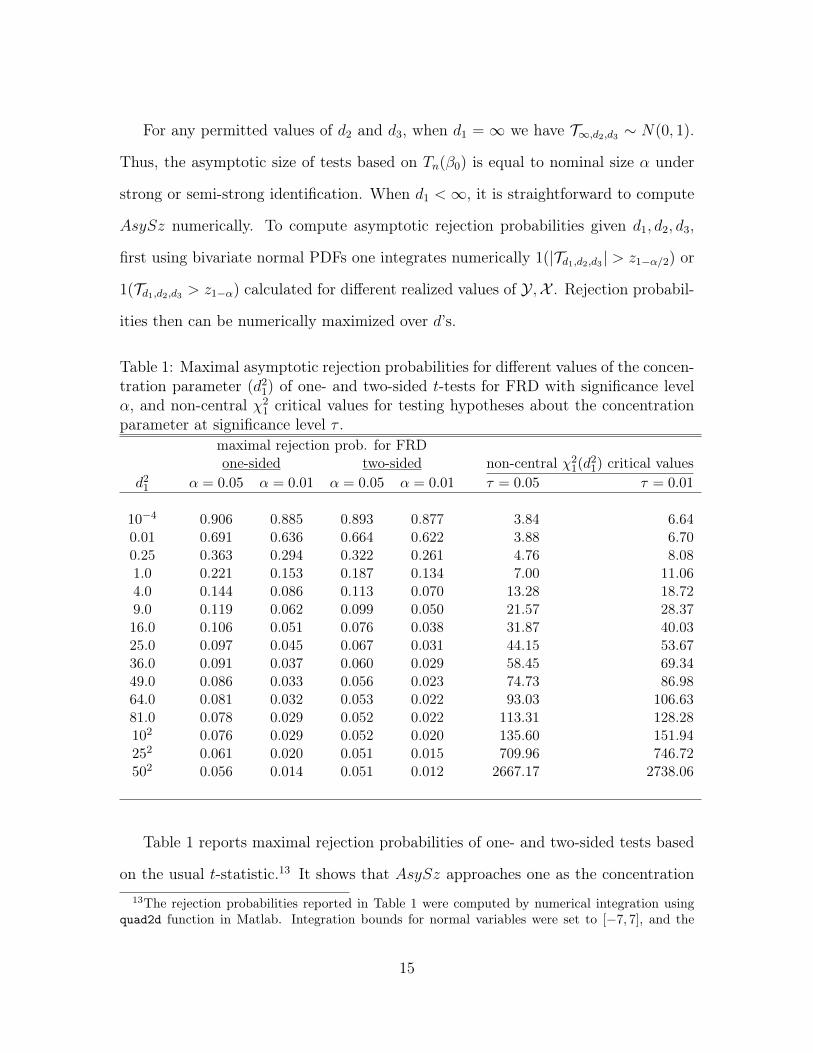
Table 1: Maximal asymptotic rejection probabilities for different values of the concen-tration parameter (d2

1) of one- and two-sided t-tests for FRD with significance levelα, and non-central χ2

1 critical values for testing hypotheses about the concentrationparameter at significance level τ .

maximal rejection prob. for FRDone-sided two-sided non-central χ2

1(d21) critical values

d21 α = 0.05 α = 0.01 α = 0.05 α = 0.01 τ = 0.05 τ = 0.01

10−4 0.906 0.885 0.893 0.877 3.84 6.640.01 0.691 0.636 0.664 0.622 3.88 6.700.25 0.363 0.294 0.322 0.261 4.76 8.081.0 0.221 0.153 0.187 0.134 7.00 11.064.0 0.144 0.086 0.113 0.070 13.28 18.729.0 0.119 0.062 0.099 0.050 21.57 28.3716.0 0.106 0.051 0.076 0.038 31.87 40.0325.0 0.097 0.045 0.067 0.031 44.15 53.6736.0 0.091 0.037 0.060 0.029 58.45 69.3449.0 0.086 0.033 0.056 0.023 74.73 86.9864.0 0.081 0.032 0.053 0.022 93.03 106.6381.0 0.078 0.029 0.052 0.022 113.31 128.28102 0.076 0.029 0.052 0.020 135.60 151.94252 0.061 0.020 0.051 0.015 709.96 746.72502 0.056 0.014 0.051 0.012 2667.17 2738.06

Table 1 reports maximal rejection probabilities of one- and two-sided tests based

on the usual t-statistic.13 It shows that AsySz approaches one as the concentration13The rejection probabilities reported in Table 1 were computed by numerical integration using

quad2d function in Matlab. Integration bounds for normal variables were set to [−7, 7], and the

15

parameter approaches zero. Size distortions decrease monotonically as the concentra-

tion parameter increases. In the case of two-sided testing, nearly zero size distortions

(under 0.5%) correspond to the concentration parameter of order d21 ≥ 64 for asymp-

totic 5% tests, and d21 ≥ 502 for asymptotic 1% tests. The table also shows that

one-sided tests suffer from more substantial size distortions than two-sided tests,

which is due to asymmetries in the distribution of Td1,d2,d3 .

2.3 Testing for potential size distortions

Following the approach of Stock and Yogo (2005), Table 1 can be used for testing a null

hypothesis about the largest potential size distortion against an alternative hypothesis

under which the largest potential size distortion does not exceed a certain pre-specified

level. Suppose that the econometrician decides that identification is strong enough

if, in the case of 1% two-sided testing, the maximal rejection probability does not

exceed 5%. Thus, the econometrician effectively adopts tests with 5% significance

level, however uses the 1% standard normal critical value. According to the results

in Table 1, the corresponding null hypothesis and its alternative in this case can be

stated in terms of the concentration parameter d21 as HW

0 : d21 ≤ 9 and HS

1 : d21 > 9

respectively. A test of HW0 can be based on the estimator of discontinuity ∆x. Define

Fn =nhn(∆xn)2

σ2x,nk/fz,n(z0)

= ((∆Xn/σx) + dn,1)2 + op(1). (8)

As long as the concentration parameter is finite, Fn →d χ21(d2

1), a non-central χ21

distribution with non-centrality parameter d21. Let χ2

1,1−τ (d21) denote the (1 − τ)-th

quantile of the χ21(d2

1) distribution. Since size distortions are monotonically decreasing

rejection probabilities were maximized over the following grids of values: from −0.99 to 0.99 at 0.01intervals for d2, and from −1000 to 1000 at 0.5 intervals for d3.

16

when the concentration parameter increases, an asymptotic size τ test of HW0 should

reject it when Fn > χ21,1−τ (d

21).

Non-central χ21 critical values are reported in the last two columns of Table 1

for selected values of the concentration parameter and τ = 0.05, 0.01. For example,

HW0 : d2

1 ≤ 9 should be rejected in favor of HS1 : d2

1 > 9 by a 5% test when Fn > 21.57.

In the case of 5% two-sided testing of β, one needs the concentration parameter of at

least 64 to ensure that size distortions are under 0.5%. In that case, a 5% test should

reject the null hypothesis of weak identification if Fn > 93.03.

Note that the critical values in Table 1 substantially exceed the rule-of-thumb of

10, which is often used in the literature as a threshold value for weak IVs. According

to our calculations, with an F -statistic of only 10, one cannot reject HW0 : d2

1 ≤ 1.512

at 5% significance level. However, a concentration parameter of 1.512 corresponds to

maximal rejection probabilities of 16.9% and 13.6% for 5% one-sided and two-sided

tests respectively.

The results from Table 1 can also be used for designing valid tests (for the FRD

effect β) based on usual t-statistics in combination with somewhat larger than usual

critical values. For example, suppose one is interested in a 5% two-sided test about

β, and rejects the null hypothesis when Fn > 21.57 and |Tn(β0)| exceeds the 1%

standard normal critical value. According to Table 1, if the concentration parameter

d21 ≥ 9, the asymptotic size does not exceed 5%. On the other hand, if d2

1 ≤ 9,

limn→∞ P (Fn > 21.75) ≤ 0.05. Hence, overall this test has an asymptotic 5% sig-

nificance level. Intuitively, such a test is valid because the null-hypothesis for the

F -pre-test assumes size distortions, and one proceeds using the t-statistic only if it

is rejected, i.e. if the concentration parameter is found to be large enough. Note,

however, that the procedure is conservative. Furthermore, passing the F -test does

not completely safeguard against size distortions, and the usual t-statistic must be

17

used with somewhat larger critical values.

Although the F -test provides useful guidance on the potential magnitude of size

distortions, practitioners should not solely rely on this test to decide whether it is

worth proceeding with the estimation. With this in mind, we present a robust in-

ference approach in the next section that always yields valid confidence intervals

regardless of the strength of identification and does not rely on any pre-tests.

2.4 Weak-identification-robust inference for FRD

A common approach adopted in the weak IVs literature is to use weak-identification-

robust statistics to test hypotheses about structural parameters directly, instead of

using their estimates and standard errors. The Anderson-Rubin (AR) statistic (An-

derson and Rubin, 1949; Staiger and Stock, 1997) is often used for that purpose. In

the context of IV regression, the AR statistic can be used to test H0 : β = β0 against

H1 : β 6= β0 by testing whether the null-restricted residuals computed for β = β0 are

uncorrelated with the instruments.

In our case, the structural parameter is defined by (1). Hence, to test H0 : β = β0

against H1 : β 6= β0, following the AR approach we can test instead H0 : ∆y−β0∆x =

0 against H1 : ∆y − β0∆x 6= 0. A test, therefore, can be based on

nhn

(∆yn − β0∆xn

)2

kσ2n(β0)/fz,n(z0)

=∣∣TRn (β0)

∣∣2 ,where TRn (β0) denotes a modified or null-restricted version of the usual t-statistic:

TRn (β0) =√nhn

(βn − β0

)/

√kσ2

n(β0)/(fz,n(z0)(∆xn)2),

and the equality holds by (4). Unlike the usual t-statistic, TRn (β0) uses the null-

18

restricted value β0 instead of βn when computing the standard error. In view of the

discussion at the beginning of Section 2.2 and since the asymptotic distribution of

|TRn (β0)| does not depend on the concentration parameter, replacing σ2n(βn) by σ2

n(β0)

eliminates size distortions.

Theorem 5. Suppose that Assumption 2 holds. Tests that reject H0 : β = β0 in favor

of H1 : β 6= β0 when |TRn (β0)| > z1−α/2 have AsySz equal to α.

Consider now a one-sided testing problem H0 : β ≤ β0 vs. H1 : β > β0. Again,

one can base a test on the null-restricted statistic. In this case under H0 when

β = β0 we have TRn (β) = (∆Yn − β∆Xn) × sign (∆Xn ± dn,1) /σ(β) + op(1). When

identification is strong or semi-strong, dn,1 → ∞, and the sign term is constant

with probability one. Since the first term is asymptotically N(0, 1), TRn (β) is also

asymptotically N(0, 1), and one could use standard normal critical values. On the

other hand, when identification is weak and the concentration parameter is small, the

sign term is random, and therefore, the null asymptotic distribution of the product

differs from the standard normal. To obtain an asymptotically uniformly valid test,

one can use data-dependent critical values that automatically adjust to the strength

of identification. Such critical values can be generated using the approach of Moreira

(2001, 2003) by conditioning on a statistic that is i) asymptotically independent of

∆Yn− β∆Xn, and ii) summarizes the information on the strength of identification.14

Define Sn = (∆Yn − β∆Xn)/σ(β) and Q = ∆Xn/σx − (σxy − βσ2x)Sn/(σxσ(β)),

so that, when β = β0, TRn (β) = Sn × sign[Qn ± dn,1 + (σxy − βσ2x)Sn/(σxσ(β))] +

op(1). When identification is weak, Sn and Qn are asymptotically independent by

construction, while Sn →d N(0, 1). Therefore one can construct data-dependent14See also Andrews et al. (2006) and Mills et al. (2014).

19

critical values as follows. First, compute

Qn(β0) =

√nhn∆xn√

kσ2x,n/fz,n(z0)

−σxy,n − β0σ

2x,n

σx,nσn(β0)

√nhn(

∆yn − β0∆xn

)√kσ2

n(β0)/fz,n(z0)

.

Second, simulate M independent N(0, 1) random variables {S1, . . . ,SM} for some

large M . Third, for m = 1, . . .M compute

T Rn,m(β0, Qn(β0)) = Sm × sign

(Qn(β0) +

σxy,n − β0σ2x,n

σx,nσn(β0)Sm).

Let cvn,1−α(β0, Qn(β0)) denote the (1 − α)-th quantile of the sample distribution of

{T Rn,m(β0, Qn(β0)) : m = 1, . . . ,M}. To obtain an asymptotically uniformly valid

one-sided test, one can use cvn,1−α(β0, Qn(β0)) as the critical value.

Theorem 6. Suppose that Assumption 2 holds. Tests that reject H0 : β ≤ β0 in favor

of H1 : β > β0 when TRn (β0) > cvn,1−α(β0, Qn(β0)) have AsySz equal to α.

Weak-identification-robust confidence sets for β can be constructed by inversion

of the robust tests. For example, a confidence set for β with asymptotic coverage

probability 1−α can be constructed by collecting all values β0 that cannot be rejected

by the two-sided robust test:

CS1−α,n ={β0 ∈ R :

∣∣TRn (β0)∣∣ ≤ z1−α/2

}. (9)

This confidence set can be easily computed analytically by solving for values of β0

that satisfy the inequality

(βn − β0)2σ2x,nFn − z2

1−α/2(σ2y,n + β2

0 σ2x,n − 2σxy,nβ0) ≤ 0, (10)

20

where Fn is defined in (8).

Depending on the coefficients of the second-order polynomial (in β0) in equation

(10), CS1−α,n can take one of the following forms: i) an interval, ii) a union of two

disconnected half-lines (−∞, a1] ∪ [a2,∞), where a1 < a2, or iii) the entire real line.

One will see cases ii) or iii) if the coefficient on β20 in (10) is negative, which occurs

when

Fn − z21−α/2 < 0. (11)

Thus, in practice one will see non-standard confidence sets if the null hypothesis

∆x = 0 cannot be rejected using the F -statistic and central χ21,1−α critical values.

Case iii) arises when the discriminant of the quadratic polynomial in (10) is negative,

which occurs if

Fnσ2n(βn)− z2

1−α/2(σ2y,n − σ2

xy,n/σ2x,n

)< 0. (12)

Positive definiteness of the variance-covariance matrix composed of σ2x,n, σ2

y,n, and

σxy,n implies that (11) holds whenever (12) holds. Thus, negative discriminants im-

plied by (12) are inconsistent with Fn > z21−α/2 or positive coefficients on β2

0 in (10).

This in turn implies that CS1−α,n cannot be empty.

When identification is strong or semi-strong, the concentration parameter and,

therefore, Fn diverge to infinity. In such cases, both the discriminant and the coef-

ficient on β20 tend to be positive, and consequently, CS1−α,n will be an interval with

probability approaching one.

Furthermore, one can show that when identification is strong and under local

alternatives of the form β = β0 + µ/(nhn)1/2, tests based on Tn(β0) and TRn (β0) have

the same asymptotic power. Thus, in practice there is no loss of asymptotic power

from adopting the robust inference approach if identification is strong.

21

3 Testing for constancy of the RD effect across co-

variates

In this section, we develop a test of constancy of the RD effect across covariates, which

is robust to weak identification issues. Such a test can be useful in practice when

the econometrician wants to argue that the treatment effect is different for different

population sub-groups. For example, in Section 4 we use this test to argue that the

effect of class sizes on educational achievements is different for secular and religious

schools, and therefore it might be optimal to implement different rules concerning

class sizes in those two categories of schools.15

Similarly to Otsu et al. (forthcoming), we consider the RD effect conditional on

some covariate wi.16 Let W denote the support of the distribution of wi. Next, for

w ∈ W we define y+(w) using the conditional expectation given zi and wi = w:

y+(w) = limz↓z0 E (yi|zi = z, wi = w) . Let y−(w), x+(w) and x−(w) be defined sim-

ilarly. The conditional RD effect given wi = w is defined a sβ(w) = (y+(w) −

y−(w))/(x+(w) − x−(w)). Similarly to the case without covariates, under an appro-

priate set of assumptions, β(w) captures the (local) ATE at z0 conditional on wi = w.

We are interested in testing the null hypothesis of constancy of the RD effect

H0 : β(w) = β for some β ∈ R and all w ∈ W , (13)

against a general alternative H1 : β(w) 6= β(v) for some v, w ∈ W . When identifi-

cation is strong, the econometrician can estimate the conditional RD effect function

consistently and then use it for testing of H0.17 However, this approach can be unre-15The problem is related to the classical ANOVA hypothesis of homogeneous populations (see, for

example, Casella and Berger, 2002, Chapter 11).16See also Frölich (2007).17Such a test can be constructed similarly to the ANOVA F -test as in Casella and Berger (2002,

22

liable if identification is weak. We therefore take an alternative approach.

Suppose that W = {w1, . . . , wJ}, i.e. the covariate is categorical and divides

the population into J groups. The assumption of a categorical covariate is plausible

in many practical applications where the econometrician may be interested in the

effect of gender, school type, etc. However, even when the covariate is continuous,

in a nonparametric framework it might be sensible to categorize it to have sufficient

power (as is often done in practice). For j = 1, . . . , J , let y+n (wj), y−n (wj), x+

n (wj),

and x−j,n(wj) denote the local linear estimators of the corresponding population terms

computed using only the observations with wi = wj. Let nj be the number of such

observations. σ2y(w

j), σ2x(w

j) and σxy(wj) are defined as the conditional versions of

the corresponding population terms, and σ2y,n(wj), σ2

x,n(wj), and σxy,n(wj) denote the

corresponding estimators.

Suppose that Assumption 2 holds for each of the J categories, and none of the

categories is redundant asymptotically: njhnj/(nhn)→ pj > 0 for j = 1, . . . , J , where

n =∑J

j=1 nj. IfH0 is true and the FRD effect is independent of w, one can construct a

robust confidence set for the common effect: CSJ1−α,n ={β0 ∈ R : Gn(β0) ≤ χ2

J,1−α},

where

Gn(β0) =J∑j=1

njhnj

(βn(wj)− β0

)2

kσ2n(β0, wj)/(fz,n(z0|wj)(∆xn(wj))2)

,

βn(wj) = ∆yn(wj)/∆xn(wj), ∆xn(wj) = x+n (wj)− x−n (wj); σ2

n(β0, wj) is defined sim-

ilarly to σ2n(β0) in (3) using the estimators conditional on wi = wj; and fz,n(z0|wj) =

(njhnj)−1∑n

i=1K((zi − z0)/hnj)1{wi = wj} is the estimator for fz(z0|wj), which de-

notes the conditional density of zi at z0 conditional on wi = wj.

Under H0 : β(w) = β for some β ∈ R, CSJ1−α,n is an asymptotically valid confi-

Chapter 11) and is discussed in the supplement.

23

dence set since Gn(β) →d χ2J under weak or strong identification. We consider the

following size α asymptotic test: Reject H0 if CSJ1−α,n is empty. The test is asymp-

totically valid because under H0, P (CSJ1−α,n = ∅) ≤ P (β /∈ CSJ1−α,n) = P (Gn(β) >

χ2J,1−α) → α, which again holds under weak or strong identification. Under the al-

ternative, there is no common value β that will provide a proper re-centering for

all J categories, and therefore, one can expect deviations from the asymptotic χ2J

distribution.

We show below that the test is consistent if there is strong (or semi-strong) iden-

tification for at least two values wj1 and wj2 that satisfy β(wj1) 6= β(wj2). Let

d2n,1(wj) = njhnj

|x+(wj)− x−(wj)|2fz(z0|wj)/(kσ2x(w

j)) be the conditional version of

the concentration parameter.

Theorem 7. Suppose that njhnj/(nhn) → pj > 0 and Assumption 2 holds for each

j = 1, . . . , J .

(a) Tests that reject H0 of constancy in (13) when CSJ1−α,n = ∅ have AsySz less or

equal to α.

(b) Let W∗ = {w1, . . . , wJ∗} ⊂ W be such that d2

n,1(wj) → ∞ for wj ∈ W∗ and

β(wj1) 6= β(wj2) for some wj1 , wj2 ∈ W∗. Then, P (CSJ1−α,n = ∅) → 1 as

n→∞.

4 Empirical Applications

In this section we compare the results of standard and weak identification robust

inference in two separate, but related, applications. We show that the standard

method and our proposed method yield significantly different conclusions when weak

identification is a problem, but similar results when it is not. We also show that

24

Figure 1: Angrist and Lavy (1999): Empirical relationship between class size andschool enrollment

Note: The solid line show the relationship when Maimonides’ rule (cap of 40 students) is

strictly enforced.

the robust confidence sets can provide more informative answers than the standard

confidence intervals in cases when the usual assumptions are violated. We also apply

our weak identification robust constancy test.

We begin with a case where weak identification is not a serious issue. In an

influential paper, Angrist and Lavy (1999) study the effect of class size on academic

success in Israel using the fact class size in Israeli public schools was capped at 40

students during their sample period. As demonstrated in Figure 1, this cap results

in discontinuities in the relationship between class size and total school enrollment

for a given grade. In practice, school enrollment does not perfectly predict class size

and thus the appropriate design is fuzzy rather than sharp. We use the same sample

selection rules as Angrist and Lavy (1999) and focus on language scores among 4th

graders.18

Table 2 shows that the estimated discontinuity in the treatment variable (the18The data can be found at http://econ-www.mit.edu/faculty/angrist/data1/data/anglavy99.

There is a total of 2049 classes in 1013 schools with valid test results. Here we only look at the firstdiscontinuity at the 40 students cutoff. The number of observations used in the estimation dependson the bandwidth. It ranges from 471 classes in 118 schools for the smallest bandwidth (6), to 722observations in 484 schools for the widest bandwidth (20). We use the uniform kernel in all cases.

25

estimate of strength of identification) ranges from 8 to 14 students depending on the

bandwidth chosen. The table also shows that, as expected, the F -statistic becomes

smaller as the bandwidth gets smaller. Silverman’s normal rule of thumb and the

optimal bandwidth procedure of Imbens and Kalyanaraman (2012) both suggest a

bandwidth value of approximately 8, which corresponds to a relatively large value

of the F -statistic (approximately 62). Applying the standards of Table 1, we then

conclude that weak identification is not a serious concern in this application. Using the

5% non-central χ2 critical value, we reject the null hypothesis that the concentration

parameter is below 36, and therefore, the maximal size distortions of the 5% two-sided

tests are expected to be under 1%. Note that even at the smallest bandwidth, the

F -statistic is relatively large. This is consistent with Figure 2 which shows that the

95% standard and robust confidence sets for the class size effect are very similar. The

figure shows that the two sets of confidence intervals are essentially indistinguishable

for larger bandwidths, and only differ slightly for smaller bandwidths.

Figure 2: Angrist and Lavy (1999): 95% confidence intervals for the effect of classsize on verbal test scores for different values of the bandwidth

Note: This figure is for the enrollment cut-off of 40. The bandwidth according to Silver-man’s normal rule-of-thumb is 7.94. The optimal bandwidth selected according to Imbensand Kalyanaraman (2012) is 7.90. The scores are given in terms of standard deviationsfrom the mean.

26

Table 2: Angrist and Lavy (1999): Estimated discontinuity in the treatment variablefor the first cutoff and their standard errors, estimated effect of class size on classaverage verbal score, and standard and robust 95% confidence sets (CSs) for the classsize effect for different values of the bandwidth

bandwidth discont. std errors F -stat effect standard CS robust CS6 −8.40 1.60 27.5 −0.07 [−0.145, 0.007] [−0.170,−0.000]8 -9.90 1.26 61.9 −0.07 [−0.129,−0.015] [−0.138,−0.019]10 -10.83 1.03 110.2 −0.06 [−0.103,−0.015] [−0.103,−0.015]12 -12.00 0.92 172.0 −0.02 [−0.056, 0.011] [−0.058, 0.010]14 -12.62 0.78 258.8 −0.03 [−0.061, 0.000] [−0.062,−0.000]16 -13.21 0.69 370.1 −0.02 [−0.048, 0.008] [−0.049, 0.007]18 -13.87 0.61 525.8 −0.02 [−0.046, 0.003] [−0.047, 0.003]20 -14.35 0.56 667.7 −0.02 [−0.042, 0.005] [−0.043, 0.004]

Note: Silverman’s normal rule-of-thumb bandwidth is 7.84 and the optimal bandwidth suggested by

Imbens and Kalyanaraman (2012) is 7.90. The scores are given in terms of standard deviations from

the mean.

In this application we also compare the results of the standard constancy test of the

treatment effect across sub-groups to the results of our robust constancy test. The first

set of results reported in Section 5 of the online Supplement compare the treatment

effect for secular and religious schools. The null hypothesis (the treatment effect is

the same across subgroups) can never be rejected using a standard test. By contrast,

the robust constancy test rejects the null hypothesis for the largest values of the

bandwidth (18 and 20). We reach similar conclusions when comparing the treatment

effect for schools with above and below median proportions of disadvantaged students.

The null hypothesis is rejected by the robust test under the largest bandwidth (20).

This suggests that our proposed test may have greater power against alternatives

than the standard test in some contexts.

The second application considers a similar policy in Chile originally studied by

Urquiola and Verhoogen (2009).19 In this application, the class sizes are capped at 4519It should be noted that Urquiola and Verhoogen (2009) are not attempting to provide causal

27

students. Figure 3 shows the fuzzy discontinuity in the empirical relationship between

class size and enrollment at the various multiples of 45. The figure also shows that the

discontinuity becomes smaller as enrollment increases. In this example, the outcome

variable is average class scores on state standardized math exams and we restrict

attention to 4th graders. We also strictly adhere to the sample selection rules used

by Urquiola and Verhoogen (2009).20

Figure 3: Urquiola and Verhoogen (2009): Empirical relationship between class sizeand enrollment

Note: The solid line show the relationship when the rule (cap of 45 students) is strictlyenforced.

Table 3 reports the FRD estimates and the confidence sets for the different values

of the bandwidth and cutoff points. As before, we set the size of the test at 5%.

Starting with the first cutoff point, Table 3 shows that the robust and conventional

confidence sets diverge dramatically as the bandwidth gets smaller. Interestingly,

while the robust confidence interval is much wider than the conventional one, it

estimates of the effect of class size on tests score. They instead show how the RD design can beinvalid when there is manipulation around the cutoff, which results in a violation of Assumption 1b(exogeneity of zi). So while this particular application is useful for illustrating some pitfalls linkedto weak identification in a FRD design, the results should be interpreted with caution.

20The total number of observations is 1,636. The effective number of observations varies with thebandwidth and the enrollment cutoff of interest. At the first cutoff point (45) we use between 273 and778 school level observations, depending on the bandwidth. The range in the number of observationsis 201 to 402, 45 to 95, and 17 to 34 at the 90, 135, and 180 enrollment cutoffs, respectively. Theuniform kernel is used to compute all the results below.

28

nevertheless rejects the null hypothesis that the effect of class size is equal to zero

while the conventional fails to reject the null.

Table 3: Urquiola and Verhoogen (2009): The estimated effect of class size on theclass average math score and its 95% standard and robust confidence sets (CSs) fordifferent values of the bandwidth

bandwidth estimated effect standard CS robust CS

first cutoff (45)6 0.146 [−0.061, 0.353] (−∞,−0.433] ∪ [0.043,∞)

8 3.378 [−74.820, 81.576] (−∞,−0.120] ∪ [0.129,∞)

10 −0.437 [−1.867, 0.993] (−∞,−0.078] ∪ [0.181,∞)

12 −0.173 [−0.360, 0.014] [−1.720,−0.065]14 −0.136 [−0.246,−0.026] [−0.376,−0.060]16 −0.091 [−0.153,−0.029] [−0.186,−0.042]18 −0.073 [−0.115,−0.031] [−0.127,−0.037]20 −0.063 [−0.099,−0.027] [−0.107,−0.032]

second cutoff (90)6 0.128 [−0.025, 0.281] [0.004, 3.093]

8 0.261 [−0.061, 0.582] (−∞,−0.587] ∪ [0.085,∞)

10 0.227 [−0.111, 0.566] (−∞,−0.241] ∪ [0.046,∞)

12 0.306 [−0.296, 0.908] (−∞,−0.118] ∪ [0.053,∞)

14 0.486 [−1.092, 2.063] (−∞,−0.056] ∪ [0.068,∞)

16 1.636 [−18.745, 22.017] (−∞, 0.002] ∪ [0.065,∞)

18 −1.056 [−10.968, 8.856] (−∞,∞)

20 −0.425 [−2.041, 1.190] (−∞, 0.005] ∪ [0.162,∞)

Silverman’s rule-of-thumb bandwidth is 8.59. The optimal bandwidth suggested by Imbens and

Kalyanaraman (2012) for the cut-off of 45 is 9.67 and for the cut-off of 90, the suggested bandwidth

is 11.60. The scores are given in terms of standard deviations from the mean.

29

Table 3: (Continued)bandwidth estimated effect standard CS robust CS

third cutoff (135)6 −2.145 [−15.627, 11.336] (−∞,−0.076] ∪ [0.584,∞)

8 −0.298 [−0.692, 0.097] [−21.482, 0.007]10 −0.307 [−0.850, 0.236] (−∞, 0.027] ∪ [1.414,∞)

12 −0.309 [−0.861, 0.243] (−∞, 0.027] ∪ [1.550,∞)

14 −0.328 [−0.885, 0.228] (−∞,−0.001] ∪ [1.838,∞)

16 −0.231 [−0.652, 0.190] (−∞, 0.034] ∪ [1.604,∞)

18 −0.181 [−0.500, 0.138] (−∞, 0.041] ∪ [21.933,∞)

20 −0.136 [−0.389, 0.117] [−1.642, 0.063]fourth cutoff (180)

10 0.048 [−0.119, 0.216] (−∞, ∞)12 0.035 [−0.130, 0.200] (−∞, ∞)14 −0.047 [−0.371, 0.278] (−∞, ∞)16 −0.045 [−0.343, 0.254] (−∞, ∞)18 −0.039 [−0.316, 0.238] (−∞, ∞)20 −0.029 [−0.299, 0.242] (−∞, ∞)

Silverman’s rule-of-thumb bandwidth is 8.59 . The optimal bandwidth suggested by Imbens and

Kalyanaraman (2012) for the cut-off of 135 is 14.12 and for the cut-off of 180, the suggested bandwidth

is 17.81. The scores are given in terms of standard deviations from the mean.

To help interpret the results, we also graphically illustrate the difference between

standard and robust confidence sets in Figure 4. The first panel plots the standard

confidence sets as a function of the bandwidth. The second panel does the same for

the weak identification robust method. The shaded area is the region covered by the

confidence sets. As the bandwidth increases, the robust confidence sets evolve from

two disjoint sections of the real line to a well defined interval.21 This is consistent

with the size of the discontinuity in class size as a function of enrollment estimated

at different bandwidths and the corresponding F -statistic. At bandwidths below

10, the estimated discontinuity is small and the F -statistic is below 7. However21Note that class size is a discrete rather than a strictly continuous variable, hence the break

between bandwidths 11 and 12 when the robust confidence set switches from two disjoint half linesto a single interval.

30

at bandwidths higher than 12, the estimated discontinuity is progressively closer to

10 students and the F -statistic ranges from just over 40 to just over 188. This is

important since the bandwidth suggested by Silverman’s normal rule-of-thumb is

only 8.59 and the optimal bandwidth suggested by Imbens and Kalyanaraman (2012)

is 9.67. See Section 5 in the online supplement for a complete listing of the F -statistic

and discontinuity estimates at different bandwidths.

Figure 4: Urquiola and Verhoogen (2009): 95% standard and robust confidence sets(CSs) for the effect of class size on class average math score for different values of thebandwidth

Note: This figure is for the first enrollment cut-off of 45. The bandwidth according to Silver-man’s normal rule-of-thumb is 8.59 . The optimal bandwidth selected according to Imbensand Kalyanaraman (2012) is 9.67. The scores are given in terms of standard deviationsfrom the mean.

Identification is considerably weaker for the second cutoff point. At all band-

widths, the standard confidence intervals fail to reject the null that the effect of class

size is zero. However, for most bandwidths, the robust confidence sets do not in-

clude a zero effect. For example, for a bandwidth of 8 we cannot reject the null that

class size is not related to grades when using the standard method, while the robust

method suggests rejecting the null.

31

Identification is even weaker at the third cutoff and, for most bandwidths, the

robust confidence sets consists of two disjoint intervals. Finally, results get very

imprecise at the fourth cutoff and the robust confidence sets now map the entire real

line. This suggests that identification is very weak at these levels and the standard

confidence sets are overly liberal, even if they do not lead the econometrician to reject

the null hypothesis of zero effects at conventional levels.

In summary, our results suggest that when weak identification is not a problem,

the robust and standard confidence sets are similar. But when the discontinuity in the

treatment variable is not large enough, the robust confidence sets are very different

from those obtained using the standard method. We also demonstrate that our robust

inference method provides more informative results than the standard method.

References

Anderson, T. W. and H. Rubin (1949): “Estimation of the parameters of a single

equation in a complete system of stochastic equations,” Annals of Mathematical

Statistics, 20, 46–63.

Andrews, D. W. K. and X. Cheng (2012): “Estimation and Inference With Weak,

Semi-Strong, and Strong Identification,” Econometrica, 80, 2153–2211.

Andrews, D. W. K., X. Cheng, and P. Guggenberger (2011): “Generic Re-

sults for Establishing the Asymptotic Size of Confidence Sets and Tests,” Cowles

Foundation Discussion Paper 1813.

Andrews, D. W. K. and P. Guggenberger (2010): “Asymptotic Size and a

Problem with Subsampling and with the m out of n Bootstrap,” Econometric The-

ory, 26, 426–468.

32

Andrews, D. W. K., M. J. Moreira, and J. H. Stock (2006): “Optimal In-

variant Similar Tests For Instrumental Variables Regression,” Econometrica, 74,

715–752.

Andrews, D. W. K. and J. H. Stock (2007): “Inference with Weak Instru-

ments,” in Advances in Economics and Econometrics, Theory and Applications:

Ninth World Congress of the Econometric Society, ed. by R. Blundell, W. K. Newey,

and T. Persson, Cambridge, UK: Cambridge University Press, vol. III.

Angrist, J. D. and V. Lavy (1999): “Using Maimonides’ Rule to Estimate The

Effect of Class Size on Scholastic Achievement,” Quarterly Journal of Economics,

114, 533–575.

Antoine, B. and P. Lavergne (forthcoming): “Conditional Moment Models Un-

der Semi-Strong Identification,” Journal of Econometrics.

Antoine, B. and E. Renault (2009): “Efficient GMM with Nearly-Weak Instru-

ments,” Econometrics Journal, 12, S135–S171.

——— (2012): “Efficient Minimum Distance Estimation with Multiple Rates of Con-

vergence,” Journal of Econometrics, 170, 350–367.

Arai, Y. and H. Ichimura (2013): “Optimal Bandwidth Selection for Differences

of Nonparametric Estimators with an Application to the Sharp Regression Discon-

tinuity Design,” Working Paper, National Graduate Institute for Policy Studies.

Bound, J., D. A. Jaeger, and R. M. Baker (1995): “Problems with Instrumen-

tal Variables Estimation When the Correlation Between the Instruments and the

Endogenous Explanatory Variable Is Weak,” Journal of the American Statistical

Association, 90, 443–450.

33

Buddelmeyer, H. and E. Skoufias (2004): “An Evaluation of the Performance

of Regression Discontinuity Design on PROGRESA,” World Bank Policy Research

Working Paper 3386.

Calonico, S., M. D. Cattaneo, and R. Titiunik (2014): “Robust Nonparamet-

ric Bias-Corrected Inference in the Regression Discontinuity Design,” Econometrica,

82, 2295–2326.

Caner, M. (2009): “Testing, Estimation in GMM and CUE with Nearly-Weak Iden-

tification,” Econometric Reviews, 29, 330–363.

Casella, G. and R. L. Berger (2002): Statistical Inference, Duxbury Press,

Pacific Grove, CA, second ed.

Davidson, J. (1994): Stochastic Limit Theory, New York: Oxford University Press.

Dong, Y. and A. Lewbel (2010): “Regression Discontinuity Marginal Threshold

Treatment Effects,” Working Paper.

Dufour, J.-M. (1997): “Some Impossibility Theorems in Econometrics with Appli-

cations to Structural and Dynamic Models,” Econometrica, 65, 1365–1387.

Fe, E. (2012): “Efficient Estimation in Regression Discontinuity Designs via Asym-

metric Kernels,” Working Paper.

Feir, D., T. Lemieux, and V. Marmer (2015): “Supplement to “Weak Identifi-

cation in Fuzzy Regression Discontinuity Designs”,” UBC Working paper.

Frölich, M. (2007): “Regression Discontinuity Design with Covariates,” Working

Paper 2007-32, University of St. Gallen.

34

Frölich, M. and B. Melly (2008): “Quantile Treatment Effects in the Regression

Discontinuity Design,” IZA Discussion Paper 3638.

Hahn, J. and G. Kuersteiner (2002): “Discontinuities of Weak Instrument Lim-

iting Distributions,” Economics Letters, 75, 325–331.

Hahn, J., P. Todd, and W. Van der Klaauw (1999): “Evaluating the Effect of

an Antidiscrimination Law Using a Regresion-Discontinuity Design,” NBER Work-

ing Paper 7131.

——— (2001): “Identification and Estimation of Treatment Effects with a Regression-

Discontinuity Design,” Econometrica, 69, 201–209.

Imbens, G. W. and K. Kalyanaraman (2012): “Optimal Bandwidth Choice for

the Regression Discontinuity Estimator,” Review of Economic Studies, 79, 933–959.

Imbens, G. W. and T. Lemieux (2008): “Regression Discontinuity Designs: A

Guide to Practice,” Journal of Econometrics, 142, 615–635.

Imbens, G. W. and C. F. Manski (2004): “Confidence Intervals for Partially

Identified Parameters,” Econometrica, 72, 1845–1857.

Imbens, G. W. and T. Zajonc (2011): “Regression Discontinuity Design with

Multiple Forcing Variables,” Working Paper.

Kleibergen, F. (2002): “Pivotal Statistics For Testing Structural Parameters in

Instrumental Variables Regression,” Econometrica, 70, 1781–1803.

Lee, D. S. and T. Lemieux (2010): “Regression Discontinuity Designs in Eco-

nomics,” Journal of Economic Literature, 48, 281–355.

35

McCrary, J. (2008): “Manipulation of the Running Variable in the Regression

Discontinuity Design: A Density Test,” Journal of Econometrics, 142, 698–714.

Mikusheva, A. (2007): “Uniform Inference in Autoregressive Models,” Economet-

rica, 75, 1411–1452.

Mills, B., M. J. Moreira, and L. P. Vilela (2014): “Tests Based on t-Statistics

for IV Regression with Weak Instruments,” Journal of Econometrics, 182, 351–363.

Moreira, M. J. (2001): “Tests with Correct Size When Instruments Can Be Arbi-

trarily Weak,” Unpublished manuscript, Department of Economics, University of

California, Berkeley.

——— (2003): “A Conditional Likelihood Ratio Test For Structural Models,” Econo-

metrica, 71, 1027–1048.

Otsu, T., K.-L. Xu, and Y. Matsushita (forthcoming): “Empirical Likelihood

for Regression Discontinuity Design,” Journal of Econometrics.

Papay, J. P., J. B. Willett, and R. J. Murnane (2011): “Extending the

Regression-Discontinuity Approach to Multiple Assignment Variables,” Journal of

Econometrics, 161, 203–207.

Porter, J. (2003): “Estimation in the Regression Discontinuity Model,” Working

Paper, University of Wisconsin–Madison.

Staiger, D. and J. H. Stock (1997): “Instrumental Variables Regression With

Weak Instruments,” Econometrica, 65, 557–586.

Stock, J. H., J. H. Wright, and M. Yogo (2002): “A Survey of Weak Instru-

ments and Weak Identification in Generalized Method of Moments,” Journal of

Business & Economic Statistics, 20.

36

Stock, J. H. and M. Yogo (2005): “Testing for Weak Instruments in Linear IV

Regression,” in Identification and Inference for Econometric Models: Essays in

Honor of Thomas Rothenberg, ed. by D. W. K. Andrews and J. H. Stock, New

York: Cambridge University Press, chap. 6, 80–108.

Urquiola, M. and E. Verhoogen (2009): “Class-size caps, sorting, and the

regression-discontinuity design,” American Economic Review, 99, 179–215.

Van der Klaauw, W. (2008): “Regression–Discontinuity Analysis: A Survey of

Recent Developments in Economics,” Labour, 22, 219–245.

37