we study reputational herding in financial markets in a … · 2016-06-18 · we study reputational...
TRANSCRIPT
econstor www.econstor.eu
Der Open-Access-Publikationsserver der ZBW – Leibniz-Informationszentrum WirtschaftThe Open Access Publication Server of the ZBW – Leibniz Information Centre for Economics
Standard-Nutzungsbedingungen:
Die Dokumente auf EconStor dürfen zu eigenen wissenschaftlichenZwecken und zum Privatgebrauch gespeichert und kopiert werden.
Sie dürfen die Dokumente nicht für öffentliche oder kommerzielleZwecke vervielfältigen, öffentlich ausstellen, öffentlich zugänglichmachen, vertreiben oder anderweitig nutzen.
Sofern die Verfasser die Dokumente unter Open-Content-Lizenzen(insbesondere CC-Lizenzen) zur Verfügung gestellt haben sollten,gelten abweichend von diesen Nutzungsbedingungen die in der dortgenannten Lizenz gewährten Nutzungsrechte.
Terms of use:
Documents in EconStor may be saved and copied for yourpersonal and scholarly purposes.
You are not to copy documents for public or commercialpurposes, to exhibit the documents publicly, to make thempublicly available on the internet, or to distribute or otherwiseuse the documents in public.
If the documents have been made available under an OpenContent Licence (especially Creative Commons Licences), youmay exercise further usage rights as specified in the indicatedlicence.
zbw Leibniz-Informationszentrum WirtschaftLeibniz Information Centre for Economics
Roider, Andreas; Voskort, Andrea
Working Paper
Reputational Herding in Financial Markets: ALaboratory Experiment
CESifo Working Paper, No. 5162
Provided in Cooperation with:Ifo Institute – Leibniz Institute for Economic Research at the University ofMunich
Suggested Citation: Roider, Andreas; Voskort, Andrea (2015) : Reputational Herding inFinancial Markets: A Laboratory Experiment, CESifo Working Paper, No. 5162
This Version is available at:http://hdl.handle.net/10419/107301

Reputational Herding in Financial Markets: A Laboratory Experiment
Andreas Roider Andrea Voskort
CESIFO WORKING PAPER NO. 5162 CATEGORY 7: MONETARY POLICY AND INTERNATIONAL FINANCE
JANUARY 2015
An electronic version of the paper may be downloaded • from the SSRN website: www.SSRN.com • from the RePEc website: www.RePEc.org
• from the CESifo website: Twww.CESifo-group.org/wp T

CESifo Working Paper No. 5162
Reputational Herding in Financial Markets: A Laboratory Experiment
Abstract We study reputational herding in financial markets in a laboratory experiment. In the spirit of Dasgupta and Prat (2008), career concerns are introduced in a sequential asset market, where wages for investors are set by subjects in the role of employers. Employers can observe investment behavior, but not investors’ ability types. Thereby, reputational incentives may arise endogenously. We find that a sizeable fraction of investors follows an established trend even in a setting where there are no reputational incentives. In a setting where there are reputational concerns, they do not seem to create substantial herd behavior.
JEL-Code: C910, D800, G140.
Keywords: reputation, herding, imitation, financial markets, experiment.
Andreas Roider*
Department of Economics University of Regensburg
Universitätsstr. 31 Germany – 93040 Regensburg
Andrea Voskort Federal Financial Supervisory Authority
(BaFin) Bonn / Germany
*corresponding author November 21, 2014 We would like to thank seminar participants at the University of Heidelberg and at the 2012 World Congress of the Game Theory Society in Istanbul. We are also grateful to a referee for very helpful comments. This paper was part of Andrea Voskort’s Ph.D. thesis at the University of Heidelberg. It represents the analysis and views of the authors and should not be thought to represent those of the German Federal Financial Supervisory Authority (BaFin).

1 Introduction
“They [equity investors] are not paid to make money, or even to beat the market.
Rather, they are paid not to do worse than their peers. Going down with the market
would not be so bad for them; missing out on a rally like in 2009, when stocks doubled in
barely two years, would be catastrophic for their career.”(Financial Times, Comment
by J. Authers, “Dangers of Market Herd Stampedes”, 30.11.2011.)
Motivation The popular press frequently alludes to herd behavior as a potential source of mis-
pricing in financial markets. Also, there is a substantial academic literature (both theoretical
and empirical) on this phenomenon. Perhaps surprisingly, even when investors are purely profit-
maximizing, herding might arise in financial markets, and market prices might fail to converge to
true values even in the long-run. One strand of the literature suggest that this might be due to
“social learning” on part of individual investors (see e.g., Park and Sabourian, 2011; Avery and
Zemsky, 1998). In particular, these authors introduce information cascade models (in the spirit
of Bikhchandani, Hirshleifer, and Welch, 1992; Banerjee, 1992; Welch, 1992) into a Glosten and
Milgrom (1985) style sequential asset market, and they show that, despite a flexible market price,
herd behavior might occur.1
As the above quotation suggests, another potential source of herd behavior are reputational
concerns of individual investors (e.g., fund managers) vis-a-vis outside observers (e.g., potential
future employers). In particular, Dasgupta and Prat (2008) introduce career concerns (in the spirit
of Scharfstein and Stein, 1990) in the Glosten and Milgrom (1985) model by assuming that investors
are of various (unobservable) ability types. In analogy to Avery and Zemsky (1998), Dasgupta and
Prat (2008) show that, following a number of trades in the same direction, the profit from trading
an asset becomes smaller because prices get more precise. At the same time, if one’s private
information runs counter to the behavior of earlier investors, acting on the own signal implies a
reputational loss, which might make it optimal to herd. Intuitively, if several predecessors have
bought the same asset, with high probability a trade contrarian to predecessors’ decisions and
1 In Avery and Zemsky (1998) this is the case in a setup with two dimensions of uncertainty and two states of the
world. Traders have private information not only about the assets’values, but also about whether some event occurs
that changes the value of the asset substantially (“event uncertainty”). While in Avery and Zemsky (1998) herding
does not emerge if there is one-dimensional uncertainty with respect to the assets’values only, Park and Sabourian
(2011) show that, even in this case, there may be herding if there are more than two states of the world.
1

according to the own signal would turn out to be unsuccessful. As a consequence, the respective
investor would incur a reputational loss as he would be considered as a low-ability investor. Hence,
it might be optimal to neglect one’s own information and to herd on predecessors’ decisions in
order not to harm one’s reputation. From that moment onwards, prices remain constant and all
subsequent investors follow the crowd.2
Of course, beyond social-learning or reputation-based explanations, there might still be other
reasons for herd behavior. For example, herding might also be driven by investors following their
“animal spirits”as Akerlof and Shiller (2008) have put it.3
Experimental setup In the present paper, we turn to the laboratory to study whether Dasgupta
and Prat’s (2008) theory of reputational herding can explain financial market behavior. Their
theory suggests that investors engage in herd behavior if they face reputational incentives and
asset prices get suffi ciently precise (i.e., profits from trading get suffi ciently small).4
In the experiment, subjects in the role of financial investors take the decision which of two
assets to buy. Subjects’investment behavior in two treatments is studied via the strategy method.
While in a treatment investment, subjects take their decisions in the absence of career concerns,
in a treatment reputation, career concerns are incorporated endogenously. For their investment
choice, investors observe investment decisions of predecessors and a signal about which asset is the
successful one. Investors can be of two types. Each investor is either a good type (and receives
an informative signal about the assets’value), or he is a bad type (and receives an uninformative
signal). Subjects are not aware of their type.
In treatment investment, the investor’s profit consists of the final payoff of the asset bought
minus the price paid for it. In this setup, according to theory, investors should always follow their
own signal and buy the respective asset. That is, there should be sincere trading only. Treatment
reputation additionally introduces principals who set wages for each investor based on the observed
investment choices and the actual outcome of the asset. Investors thus receive wages set by the
principals on top of earning profits from investing in the asset. In treatment reputation, investors
2For other theoretical work on reputational incentives in a financial markets context, see e.g., Villatoro (2009),
Dasgupta and Prat (2006), and Huddart (1999).3 Investors might, for example, have an intrinsic preference for conformity.4Herd behavior, in our setup, refers to the case in which investors follow the investment decisions of predecessors
regardless of their own signal. In this case, investors’behavior thus does not carry informational value and asset
prices do not converge to the true liquidation values.
2

should engage in herd behavior and neglect their own signal if a suffi cient number of predecessors
bought the same asset.
In the experiment, we introduce explicit wage setting by principals (as opposed to simply paying
investors a wage equal to their conditional expected productivity) because whether reputational
herding indeed emerges might, in principle, depend on two factors. Namely, on whether investors
recognize reputational incentives and whether an outside labor market indeed provides such incen-
tives.
Main insights The experimental results show that, as suggested by Dasgupta and Prat (2008),
herd behavior can be observed in treatment reputation. About half of the investors engage in
herding in the situations where it is predicted by theory. Again, as suggested by theory, in all other
situations almost all subjects trade sincerely. However, surprisingly, even in treatment investment,
herd behavior occurs to a similar extent. Hence, a substantial fraction of investors seems to follow
an established trend even in the absence of reputational incentives, and reputational concerns do
not seem to affect behavior much.
The findings of the experiment contribute to our understanding to which degree reputational
herding affects financial markets. One mechanism of how reputational concerns might influence
investment behavior has been suggested by Dasgupta and Prat (2008). Our results suggest that
this mechanism is not at work in financial markets and, hence, does not distort asset prices. Thereby,
our results complement empirical studies on financial markets (to be discussed below), which also
document only limited evidence for reputational herding.5 If the wide-spread presumption that
herd behavior is present in financial markets is true, such herd behavior might lead to substantial
mispricing of assets and misallocation of capital. Our results hint at that such herd behavior is not
driven by reputational concerns, but other (behavioral) forces might be at work (as suggested by
the imitation we observe in the experiment). To better understand these forces, more research is
warranted. Understanding the exact reasons for herd behavior is important in order to potentially
come up with ways of how to reduce this source of mispricing in financial markets.
5While an experimental approach has its own issues, it has the advantage of being able to control for decision-
makers’private information and monetary incentives (which is, in general, diffi cult when working with real financial
market data).
3

Outline The remainder of the paper is structured as follows. The related literature is discussed
in Section 2. In Section 3, we introduce Dasgupta and Prat’s (2008) model and present the theo-
retical benchmarks. In Section 4, we outline the experimental design. The experiment’s results are
discussed in Section 5 followed by concluding remarks in Section 6. In addition, we provide details
with respect to the derivation of the theoretical benchmarks (Appendix A), an English translation
of the experimental instructions (Appendix B), and an example of how individual payoffs were
calculated in the experiment (Appendix C).
2 Related literature
The present paper contributes to three strands of the literature.
Empirical literature on herd behavior in financial markets There is a substantial empirical
literature on herd behavior in financial markets (for surveys, see e.g., Bikhchandani and Sharma,
2000; Daniel, Hirshleifer, and Teoh, 2002; or Hirshleifer and Teoh, 2003). This literature has two
aims: to verify whether there is herding in financial markets, and, if yes, to investigate the reasons
for herd behavior. In particular, various authors have investigated whether, due to career concerns,
there is reputational herding by investment newsletters (see e.g., Graham, 1999), macroeconomic
forecasters (see e.g., Lamont, 2002; Ehrbeck and Waldmann, 1996), security analysts (see e.g.,
Hong and Kubik, 2003; Hong, Kubik, and Solomon, 2000; Welch, 2000), mutual fund managers
(see e.g., Massa and Patgiri, 2007; Chevalier and Ellison, 1999), or institutional investors (see e.g.,
Sias, 2004). In summary, these papers only provide mixed evidence for the presence of reputational
herding in financial markets. For example, Sias (2004) and Ehrbeck and Waldmann (1996) fail to
find evidence for reputation-driven herd behavior. Welch (2000) argues that the observed clustering
of behavior could be due to either social learning or due to reputational concerns of investors.
This empirical literature has, however, a potential shortcoming. Frequently, neither the private
information on which financial market participants act nor the performance incentives or reputa-
tional incentives they face are observable to the econometrican. Consequently, Hirshleifer and Teoh
(2003) argue that, for an empirical study, it will always be diffi cult to disentangle to which degree
reputational concerns, social learning, or simple imitation contribute to herd behavior in financial
markets. Hence, we make the following contributions to this literature. From a methodological
perspective, by conducting an experiment, we are able to control for the private information and
4

monetary incentives faced by the decision-makers; thereby circumventing the problems of empirical
studies to observe these key variables.6 Our results complement and confirm the mixed findings
of the empirical literature: we document that also under the controlled conditions of a laboratory
experiment herding due to reputational reasons seems to be rather weak. Our experiment also
shows that other (behavioral) forces seem to lead financial market participants to follow estab-
lished trends; thereby emphasizing the need to study behavioral explanations for herd behavior in
financial markets.
Experimental literature on herd behavior in financial markets There is also a recent
experimental literature on herd behavior in financial markets. These papers have not studied
reputational herding, but they have mainly focussed on settings where herding might be caused by
“social learning” (i.e. where any herding is “purely information-based”). That is, they consider
settings where the decisions of early investors might potentially reveal so much information about
an asset’s value such that, for later investors, it becomes optimal to disregard their own private
information and to follow an established herd instead.7 These studies document that, under certain
conditions, social learning indeed leads experimental subjects to engage in herd behavior; thereby
lending support to social learning as a source of herding in financial markets. For example, Park
and Sgroi (2010) lend support to Park and Sabourian (2011), whose model predicts that there might
be information-based herding in settings that are suffi ciently complex (i.e., where there are more
than two possible states of the world).8 We contribute to this experimental literature by studying
to which degree reputational concerns lead to herd behavior. In contrast to this literature, from
a theoretical perspective, social learning does not play a role in the settings we consider. Our
results provide experimental evidence that reputational forces might be of minor importance for
the emergence of herd behavior in financial markets. Instead, we find that investors tend to follow
an established trend even when there are no reputational incentives. Such simple imitation has
6Of course, as mentioned above, experimental studies might have their own issues, such as the external validity
of the findings. Hence, both approaches complement each other.7Beginning with Anderson and Holt (1997), there is a vast experimental literature on such “information cascades”
in settings with fixed prices. These studies do, however, not directly apply to financial markets where prices are
flexible. For overviews, see e.g., Weizsacker (2010) or Drehmann, Oechssler, and Roider (2007).8Note that suffi cient complexity of the environment seems to be necessary for information-based herding to emerge:
Drehmann, Oechssler and Roider (2005) and Cipriani and Guarino (2005) confirm Avery and Zemsky’s (1998) pre-
diction of no herding in a simple financial market with one-dimensional uncertainty over two potential states of the
world.
5

rarely been observed in the earlier experiments; highlighting that it might be of greater importance
than previously thought.
Experimental literature on career concerns Our paper is also related to the experimental
literature on career concerns. This literature has mostly focussed on reputational concerns in labor
markets. For example, Koch, Morgenstern, and Raab (2009) experimentally test Holmstrom’s
(1999) seminal career concerns model. In this model, through providing effort, an agent tries to
influence the beliefs of potential employers about his unknown ability, which has an impact on his
future wages. Koch, Morgenstern, and Raab (2009) find that, in line with the theoretical prediction,
reputational concerns indeed shape the agent’s behavior.9 We contribute to this literature by
studying career concerns not in a labor market context, but in a financial market. In this setting,
we find only weak evidence for the impact of reputational concerns.
3 Theoretical benchmark
3.1 Basic structure
We consider a simplified version of Dasgupta and Prat (2008) to make it suitable for a laboratory
experiment. The sequence of events is illustrated in Figures 1 and 2 below. There are four dates
t ∈ {1, 2, 3, 4} and three risk-neutral, profit-maximizing investors i ∈ {1, 2, 3}.10 Investors have to
decide sequentially which of two assets, A or B, to buy, and at date t = i it is investor i’s turn to
buy either one unit of asset A or one unit of asset B.11
Only one of the assets will turn out to have a value of 10 points (our experimental currency)
at date t = 4, while the other asset will have a value of zero points. Both states v ∈ {A,B} (i.e.,
which asset has a value of 10 points) occur with equal probability, and this is known to investors.
The state of the world is the same for all three investors. As additional information, each investor
receives a private signal si ∈ {a, b}. The signal’s precision depends on the respective investor’s
type, where each investor has an equal probability of being either “good” or “bad”. In the case
9See also the experiment by Irlenbusch and Sliwka (2006), where, however, not only career concerns, but also
gift-exchange considerations might have affected subjects’behavior.10The reasons for considering sequences of three investors are discussed in detail in Section 4.11Dasgupta and Prat (2008) consider the choice between buying or (short) selling a single asset. In line with other
experiments on herding in financial markets (see e.g., Drehmann, Oechssler, and Roider, 2005; Cipriani and Guarino,
2005) we consider the strategically equivalent choice between buying either A or B, which seems to be easier to
explain to experimental subjects.
6

of a good investor, we have σg = Prob(si = a|v = A) = Prob(si = b|v = B) = 0.9, while in the
case of a bad investor we have σb = Prob(si = a|v = A) = Prob(si = b|v = B) = 0.5. For each
investor, the signal is drawn independently conditional on the state and the investor’s type. That
is, while a good investor receives additional information by observing the signal, a bad investor’s
signal is uninformative. Denote the asset bought by investor i by V i ∈ {A,B}.12 The state of the
world as well as the investors’types are determined at the beginning of the game. Investors do not
learn their type throughout the game, and the state of the world (and hence, investors’payoffs)
is only revealed after all investment decisions have been made.13 When making his investment
decision, each investor can rely on three pieces of information: (i) his privately observed signal, (ii)
the current market prices for assets A and B, and (iii) the investment decisions of earlier investors
(if there are any) as well as the history of market prices these earlier investors have faced. How
market prices for the assets are determined is explained in more detail below.
3.2 No reputational concerns of investors
In a first step, we consider a benchmark setting where the investors do not have reputational con-
cerns because they only derive a profit from buying one of the assets. Market prices are set by a
risk-neutral, competitive market maker who effi ciently incorporates all publicly available informa-
tion, i.e., the history of trades as well as the investor’s decision to buy the respective asset. Hence,
the market price of asset A at time t is given by
ptA = 10 · Prob(A|Ht,buy A), (1)
and the price of asset B is equal to ptB = 10 · Prob(B|Ht,buy B), where Ht denotes the history of
observable decisions of all earlier investors up to time t. Other experiments (such as Drehmann,
Oechssler, and Roider, 2005; Cipriani and Guarino, 2005) have assumed that the market maker
does not condition the prices ptA and ptB on the kind of order he receives at time t (and hence, is
not fully profit-maximizing). We deviate from this and assume the price setting rule (1) because
12 In their model, Dasgupta and Prat (2008) assume that a certain fraction of the investors are noise traders whose
trading is purely random. For two reasons, we do not include such noise traders. First, this simplification does not
affect the theoretical predictions, and second, it makes it easier to explain the experimental setting to subjects. Note
that despite of this simplification, market break-down is not an issue as, in the experiment, subjects have to buy one
of the two assets. The issue of uninformed traders is discussed in more detail in the Conclusion of the paper.13Note that, in the experiment, investors learn the state and their payoffs only at the very end of the experiment
after all decisions have been made.
7

it facilitates more “extreme” prices earlier on in a given sequence of investors.14 In the current
benchmark setting, the overall payoff of investor i is given by
πiI(Vi, ptV i , v) ≡
{10− pt
V iif V i = v
−ptV i
if V i 6= v(2)
for i = t ∈ {1, 2, 3} (because investor i buys at time t = i only).
v and type ofeach investordetermined,not revealed
Investor 1enters
market andreceives
private signal
Investor 1buys asset A
or B, paysprice of asset
bought
Investor 2 entersmarket, receives
private signal andobserves decision
of investor 1
Investor 2buys asset A
or B, paysprice of asset
bought
Investor 3 entersmarket, receives
private signal andobserves decisionsof investor 1 and 2
Investor 3buys asset A
or B, paysprice of asset
bought
v revealed,payoffs realized
t=1 t=2 t=3 t=4
Figure 1: Sequence of events without reputational concerns
In line with earlier results by Glosten and Milgrom (1985) and Avery and Zemsky (1998), if
investors are only motivated by profits from trading, all trading will be sincere (i.e., all investors will
act according to their signal). Hence, investors reveal their private signal through their investment
decision to the market maker. To see this, suppose that the market maker believes that trading
has been sincere and suppose that investor i has received signal si = a. In this case, the price of A
will equal the investor’s expected value of A, and hence buying A yields the investor an expected
profit of zero. However, buying B would yield a loss because the market maker would assume that
the investor had received signal b and would set a price that exceeds the investor’s expected value
of B. Consequently, it is optimal for the investor to trade sincerely, i.e., to buy asset A (recall that
investors do not have the option not to trade). Likewise, after a signal si = b only an investment
in asset V i = B is optimal. To summarize:
Proposition 1 (Dasgupta and Prat, 2008, Section 3) In the absence of reputational concerns,
investors always follow their signal and trade sincerely, i.e., V i = A if si = a and V i = B if si = b
for all i. Prices are as in Table 1.
14 In the presence of reputational concerns (see Section 3.3 below), this will be a useful feature because, from a
theoretical perspective, “extreme”prices facilitate reputational herding.
8

Table 1: Market prices for assets A and B
t Ht ptA ptB
1 – 7.0 7.0
2 A 8.4 5.0
2 B 5.0 8.4
3 AB or BA 7.0 7.0
3 AA 9.3 3.0
3 BB 3.0 9.3
Note: Like in the experiment, prices have been rounded to the first decimal.
3.3 Investors with reputational concerns
We now augment the model as outlined in Sections 3.1 and 3.2 by reputational concerns of investors.
More precisely, in addition to the payoff from buying a certain asset, at date t = 4 each investor i
receives some wage ri that is determined at the end of the game, i.e.,
πiR ≡ πiI + ri. (3)
Investor 3 entersmarket, receives
private signal andobserves decisionsof investor 1 and 2
Investor 3 buys asset Aor B, pays price of asset
bought
Payoffsrealized
v isrevealed
Principalssubmit wagebids in a firstprice auction
t=3 t=4 t=5
Investor 3 entersmarket, receives
private signal andobserves decisionsof investor 1 and 2
Investor 3 buys asset Aor B, pays price of asset
bought
Payoffsrealized
v isrevealed
Principalssubmit wagebids in a firstprice auction
t=3 t=4 t=5
Figure 2: Sequence of events with reputational concerns
Dasgupta and Prat (2008) consider the case that investors are fund managers and that the wage
ri is given by an outside market’s posterior belief that investor i is a good type (i.e., an investor
whose signal has informational content). The outside market (i.e., potential future employers)
observes the entire history H4 of trades and prices as well as the realized true state of the world v
(i.e., which of the two assets is successful). Consequently, in contrast to Section 3.2, investors have
9

an incentive to be perceived as a good type. It will turn out that, for investor 3, it is optimal to
disregard his private signal and to herd whenever both predecessors have bought the same asset.
The intuition is as follows: If early investors follow their signal, the price incorporates their
private information and moves towards the true liquidation value. Over time, however, price
movements become smaller. In particular, profits from trading according to one’s signal stay zero,
while profits from trading against one’s signal stay negative, but decrease in absolute terms. At
the same time, a trader who observes a signal contrarian to earlier price movements (and hence,
contrarian to the most likely outcome of the asset) faces endogenous reputational costs: if he would
follow his signal, with a high probability the asset he buys would turn out to be worthless and he
would be perceived as a bad investor who had received an uninformative signal. Thus, as prices
become suffi ciently precise (and differential profits from trading A respectively B suffi ciently small),
investors start to follow predecessors out of reputational concerns.
Wage setting process by principals In practice, whether reputational herding indeed emerges
depends not only on the behavior of investors, but potentially also on the wage setting behavior
by the outside market. Consequently, while Dasgupta and Prat (2008) assume that an investor’s
wage is equal to his conditional expected productivity, we consider an explicit wage setting process
(which yields the same theoretical prediction). In particular, investor i’s wage is determined in a
sealed-bid, first-price auction among six risk-neutral, profit-maximizing “principals”, where investor
i’s wage ri is determined by the highest bid. The sequence of events is identical to Section 3.1 up
to date t = 3. As can be observed in Figure 2, it only differs from t = 4 onwards.
Principals can observe the entire history of trades and prices as well as the realized true state
of the world v. The winning principal has to pay his bid and additionally gets 20 points if and
only if investor i happens to be good (otherwise he gets no additional points).15 The remaining
five principals get a payoff of zero each.
If, at date 4, principals hold a common belief γ that investor i is of good type, the principals’
bidding strategies in the symmetric equilibrium of the first-price auction are 20 · γ (i.e., bids are
equal to the respective investor’s “expected value”).16 Hence, in analogy to Dasgupta and Prat
15 In case of a tie, each of the highest bidding principals wins with equal probability.16To see this, note that in any equilibrium the following has to hold: (i) all bids must be weakly below 20 · γ
(because otherwise the winning bid would lead to a loss), (ii) the maximum bid must be equal to 20 · γ (becauseotherwise a losing bidder would have an incentive to overbid), and (iii) at least two bids must be equal to 20 · γ
10

(2008), in equilibrium the respective investor i receives a reputational payoff of ri = 20 · γ.17
Dasgupta and Prat (2008) show that the belief γ that principals hold about a given investor
only depends on this investor’s equilibrium strategy and the realized true state of the world (but
not on the behavior of other investors). Intuitively, this is the case because principals can observe
which of the assets turns out to be successful, and investors’signals are mutually independent given
the true state of the world v (see Dasgupta and Prat, 2008, Proof of Proposition 1). Consequently,
(with one exception to be discussed below) equilibrium wage bids take on two values only:18 they
are equal to 12.86 if the respective investor chose the successful asset, and they are equal to 3.33 if
the respective investor chose the unsuccessful asset. The exception are the wage bids for an investor
3 who has invested in the same asset as both of his predecessors (i.e., if H4 ∈ {AAA,BBB}). Such
an investor engages in reputational herding, and hence his behavior is uninformative. As, from an
ex-ante perspective, both types of the investor are equally likely, such an investor 3 receives a wage
offer of 0.5 · 20 = 10.
Market prices set by the market maker The possibility of herding raises an issue with respect
to price setting by the market maker in the experiment. From a theoretical perspective, it will turn
out that, even in the presence of reputational concerns, both investor 1 and 2 trade sincerely in
equilibrium. Consequently, for them, a profit-maximizing market maker will set asset prices as spelt
out in Table 1. However, for the case of investor 3, the market maker will suspect herd behavior
if H3 ∈ {AA,BB}, and, in this case, a profit-maximizing market-maker would confront investor 3
with market prices that deviate from Table 1. In the experiment, market prices that differ across
treatments would, however, be problematic as earlier studies have shown that price levels per se
influence subjects’ inclination to follow their own signal (see e.g., Cipriani and Guarino, 2005;
Drehmann, Oechssler and Roider, 2005). In particular, there is evidence for contrarian behavior,
where subjects are more likely to act against their signal, if prices are higher. This price effect would
make it diffi cult to compare our treatments with and without reputational concerns. To rule out
this confounding effect, we assume that even if investors’payoffs are given by (3), the market maker
(because otherwise the winning bidder would have an incentive to lower his bid). Hence, in any equilibrium of the
first-price auction at least two principals bid 20 · γ, while the remaining principals bid weakly less than that.17Note that in Dasgupta and Prat (2008) the weight of reputational concerns in an investor’s payoff function is
determined by the parameter (1 − β), where β constitutes the payoff fraction from investing in the asset. By fixing
the value of the good investor to 20 and the successful asset’s payoff to 10, (1− β) equals 23in our setup.
18For a more detailed sketch of Dasgupta and Prat’s (2008) argument, see Appendix A.
11

sets market prices according to Table 1.19 In Appendix A, we illustrate that theoretical predictions
with respect to the behavior of investors and principals remain unaffected by this assumption.20
As a theoretical benchmark in the presence of reputational concerns, we focus on Dasgupta and
Prat’s (2008) “most revealing equilibrium”, in which investors maximally condition their trades on
their private information (see Dasgupta and Prat, 2008, Section 4.1):21
Proposition 2 (Dasgupta and Prat, 2008, Proposition 4) Assume that market prices are as
in Table 1 and that investors have reputational concerns. Then, in the most revealing equilibrium,
investors 1 and 2 trade sincerely. Investor 3 trades sincerely unless both of his predecessors have
invested in the same asset, in which case he herds. The (symmetric) wage bids submitted by the
principals for investor i are equal to (a) 10 if i = 3 and H4 ∈ {AAA,BBB}, and (b) otherwise
they are equal to 12.86 (3.33) if investor i has bought the successful (unsuccessful) asset.
4 Experimental design
Recruitment and subject pool The experiment was conducted in five sessions, which ran in
May and June 2011 in the AWI Lab at the University of Heidelberg. Participants were recruited
randomly via Orsee (Greiner, 2004) from AWI Lab’s subject pool of persons who had indicated
their interest in participating in economic experiments. In total, 90 subjects participated; 18 in
each session. None of the subjects had participated in experiments on either herd behavior or
reputational effects before. Each session lasted approximately 120 minutes. Participants earned
13.95 Euro on average. Altogether, 44 females (48.89%) and 46 males participated. The average
age was 21.68 years, and the average number of semesters studied 3.75. Of the participants, 35.6%
were economics majors, while the second largest group consisted of law students (12.22%). The
entire experiment was paper and pencil based.
19Recall that the role of market maker is played by the experimenter, and hence potential losses are not an issue.20 Intuitively, as argued above, equilibrium wage bids by principals for a given investor do only depend on investors’
equilibrium strategies as well as on the realized true state of the world. In Appendix A, we show that, given equilibrium
wage bidding strategies of principals, equilibrium investment strategies of investors are the same independent of
whether one sets market prices according to Table 1 or whether market prices take potential herd behavior by
investor 3 into account.21That is, in this equilibrium information is revealed in the fastest possible way in the sense that there is no other
(reasonable) equilibrium where, at any date t, more information is revealed.
12

Implementation Upon entering the laboratory, all 18 participants of a given session were in-
formed that investment decisions in two completely independent rounds had to be taken. A trans-
lation of the experimental instructions can be found in Appendix B.
In the first round, subjects played a treatment investment, and in the second round they played
a treatment reputation. The (benchmark) treatment investment corresponds to the setting without
reputational concerns described in Section 3.2. That is, all subjects acted as investors, their payoff
function was given by (2), and this was common knowledge among participants. Treatment repu-
tation corresponds to the setting with reputational concerns of investors described in Section 3.3.
Subjects learned about the details of treatment reputation only after they had completed the first
round. In each session of treatment reputation, six randomly selected subjects acted as principals,
while the remaining 12 subjects acted as investors. Investors’payoff functions were given by (3),
principals made wage offers for investors as described in Section 3.3, and again this was common
knowledge among participants. In order to ensure that both investors and principals were informed
about the entire (information) structure of the game, all subjects received identical instructions.
To achieve comparability, investors received identical decision sheets in both rounds of the experi-
ment.22 As discussed in Sections 3.2 and 3.3, in both treatments market prices for the two assets
were set according to Table 1.23
Both rounds of a session had the same basic structure. First, the instructions for the respective
round were handed to subjects and read out aloud by the experimenter. Afterwards, the experi-
menter additionally explained the main features of the respective round via a flip chart to subjects.
Subsequently, to check whether the experimental setup was clear, a questionnaire regarding details
of the setup had to be answered. Only after all subjects had filled out the questionnaire correctly,
decision sheets were distributed and filled out by the subjects. After this, the respective round
ended.
Only after the second round, subjects learned their payoffs. They also answered a post-
experimental questionnaire, where we requested demographic information, asked questions about
the experiment, and elicited subjects’ degree of risk aversion. Finally, payments were privately
22Subjects were allowed to keep a copy of their first round decision sheet as a reference for the second round.
Importantly, we made it clear to subjects that second-round decision-making did not require recalling first-round
decisions.23Drehmann, Oechssler, and Roider (2005) conduct an experiment on information-based herding in financial mar-
kets and document behavior that is quite robust across pricing rules that make different assumptions on the behavior
of investors (e.g., pricing rules that allow for different forms of “mistakes”).
13

handed out to subjects, after which the experiment ended.
Strategy method to elicit subjects’ decisions To elicit subjects’ decisions, the strategy
method was used. This design choice (together with the choice to consider sequences of three
investors) was driven by the following considerations. As discussed in Section 3.3, in the presence
of reputational concerns theory suggests sincere trading by investors 1 and 2, and it suggest herding
by investor 3 only if both of his predecessors have bought the same asset. Hence, if we would not
have employed the strategy method, only the decisions of subjects who (i) act as investor 3 and (ii)
face a history of earlier decisions H3 ∈ {AA,BB} would have been informative with respect to the
presence of reputational herding. In order to economize on the size of the subject pool, we therefore
have used the strategy method. Given this design choice, we restrict attention to sequences of three
investors in order to limit the number of decisions each subject has to take.
Translations of the decision sheets that investors and principals had to fill out can be found in
Appendix B. When acting as an investor, the respective subject was asked to state decisions V i for
all i ∈ {1, 2, 3}, for all possible histories of prices and predecessors’decisions, and all possible own
signal realizations he might observe. That is, the respective subject was asked to state a decision
for every information set at which an investor might have to make a decision. For example, when
acting as an investor the subject was asked to imagine he were investor 1 and to state his decision
for both the cases that he receives the signal s1 = a and s1 = b. Likewise, the subject was asked
to imagine he were investor 2 and to state his (in total, four) decisions depending on whether his
predecessor had chosen A or B and depending on whether his own signal was a or b. In a similar
vein, as investor 3 he had to state 8 decisions. Subjects who acted as principals in treatment
reputation were asked to submit a bid for each investor i ∈ {1, 2, 3} for each possible history of
decisions and prices the respective investor might have observed, and for each possible realization
of the state of the world.24
Payments Subjects received a show-up fee of 4 Euro about which they were informed at the
beginning of the experiment. Subjects were furthermore told that, depending on their success in
the experiment, they could earn additional money, where each additional point (our experimental
currency) paid out 0.20 Euro. In each of the two rounds, each subject (investors in treatment
24The maximum possible bid for an investor was limited to 20 points.
14

investment, and investors and principals in treatment reputation) received an initial endowment of
20 points. Except for the show-up fee, the exact amount earned was revealed at the end of the
experiment only (and subjects were aware of this).
As we employ the strategy method, in each of the two rounds each subject’s payoff depended
on one randomly chosen decision, and we took care to explain in detail to subjects how individual
payoffs were calculated. In the following, we describe how individual payoffs were calculated, and in
Appendix C, we provide an example. In particular, at the end of the experiment and independently
for each of the two rounds, payments were determined as follows: By making draws from urns, (i)
we randomly allocated investors into groups of three subjects and randomly assigned the roles of
investor 1, 2, and 3, and (ii) according to the probabilities described above, for each of the investor
groups, we randomly determined the successful asset and each investor’s type and signal.25 Given
this information, for each of the investor groups, we are then able to obtain the decision of investor 1
from the respective subject’s decision sheet and to calculate his payoff from his investment decision
(see (2) above). In a second and third step, we then obtain the decisions (and calculate the payoffs)
of investors 2 and 3 in an analogous way (given the decisions of investor 1, and of investors 1 and
2, respectively). This concludes the determination of payoffs in treatment investment.
In treatment reputation, the above procedure left us with a decision history and a successful
asset for each of the four investor groups in a given session of this treatment. By looking at the
decision sheets of principals, we were, hence, able to determine the highest bid for each investor
(i.e., his wage). Given the respective investor’s type, we were also able to determine the principals’
payoffs from the auction for the respective investor: only the winning principal had to pay the bid,
and, if the investor was a good type, the winning principal earned 20 points. All other principals
earned zero from the respective auction.26
25That is, in all of the sessions there were six investor groups in treatment investment and four investor groups in
treatment reputation.26 In both rounds, by experimental design, investors can never lose more money than the initial endowment of 20
points. If, in treatment reputation, a principal wins many auctions and happens to hire a number of investors of bad
type, he or she may, in principle, accumulate losses that exceed the initial endowment of 20 points. We excluded
this possibility by informing principals that the minimum they could earn were zero points (including the initial
endowment). While, in principle, this constraint might have given principals an incentive to overbid relative to what
is predicted by Proposition 2, we do not find evidence for this. In fact, looking at all principals, there is even evidence
for some underbidding as the average actual wage bid is equal to 6.28, while Proposition 2 would predict an average
wage bid of 8.25.
15

5 Results
In this section, the results of the experiment are presented. In Section 5.1, we discuss the evidence
for reputational herding by comparing treatments reputation and investment. Section 5.2 docu-
ments substantial imitative behavior among investors that cannot be explained by Dasgupta and
Prat’s (2008) model. Finally, in Section 5.3, we compare the actual wage setting by principals with
various benchmarks, and we study the incentives for reputational herding the actual wage setting
creates.
5.1 Evidence on reputational herding
For both treatment investment and reputation, Table 2 depicts the fraction of subjects that behave
in line with the theoretical prediction at a given information set of the game (where an information
set is characterized by the predecessors’choices and the own signal). Note that we pool information
sets that differ in labeling only, and hence are symmetric. For example, in Table 2 AAb and BBa
are both subsumed under XXy.27 More formally, in the following we describe information sets by
combinations of capital letters and small letters where capital letters refer to the observed decisions
of predecessors (i.e., X,Y ∈ {A,B}, where X 6= Y ) and small letters indicate the own signal (i.e.,.
x, y ∈ {a, b}, where x = a if X = A, x = b if X = B, y = a if X = B, and y = b if X = A).
A first inspection of Table 2 reveals that at all information sets except XXy behavior is re-
markably close to the theoretical prediction of subjects following their own signal independent of
the investment decisions of predecessors. Indeed, in treatment investment (treatment reputation)
86.39% (89.44%) of decisions are in line with theory if one averages over all information sets ex-
cept XXy.28 In treatment reputation, Dasgupta and Prat (2008) predict that investor 3 herds
at information set XXy (i.e., if the decisions of both of his predecessors conform). And indeed,
Table 2 shows that 41.67% of subjects disregard their own signal and follow the lead of predeces-
sors’decisions instead. Two observations with respect to behavior at information set XXy are,
however, surprising. First, even in treatment reputation, a majority of subjects still follows its
own signal. Second, even in treatment investment (where, according to Dasgupta and Prat (2008),
27For each pair of such symmetric information sets (and for both treatments separately), we conduct McNemar-
Change tests, which all indicate insignificant differences.28According to a Wilcoxon-Signed-Ranks test (where for each subject we compare the number of decisions that
are in line with theory in treatment investment respectively in treatment reputation), this difference is (marginally)
significant with a p-value of 0.056. This might be indicative of some learning effects across rounds.
16

Table 2: Fraction of investors behaving in line with the theoretical prediction
treatment
investor information set investment reputation
1 x 91.66 % 95.83 %
2 Xx 85.00 % 89.17 %
2 Xy 79.45 % 80.00 %
3 XXx 81.11 % 86.67 %
3 XXy 56.33 % 41.67 %
3 XY y 86.67 % 90.00 %
3 XY x 94.45 % 95.00 %
Note: N=90 (N=60) in treatment investment (reputation). With respect to the information available to subjects,
capital letters refer to the observed decisions of predecessors (i.e., X,Y∈{A,B}, where X 6=Y), and small letters indicatethe own signal (i.e.,. x,y∈{a,b}, where x=a if X=A, x=b if X=B, y=a if X=B, and y=b if X=A).
acting against one’s signal is never optimal) a substantial fraction of subjects disregards its pri-
vate information. It turns out that, both in treatment reputation and in treatment investment,
behavior differs significantly at information set XXy compared to all other information sets (at
the 1%-level).29
Table 3 investigates behavior at information set XXy in more detail. There, we restrict at-
tention to the 60 subjects that serve as investors in both treatments. As Table 3 indicates, a
substantial number of subjects either follow their own signal in both treatments (i.e., in both treat-
ments choose Y ) or follow the lead of their predecessors in both treatments (i.e., always choose
X, which, according to Table 3, holds for 43 subjects). At information set AAb (BBa) only 4 (3)
out of 60 subjects act in line with theory in both treatments. Behavior at XXy does not differ
significantly between treatments according to a McNemar-Change test.30
To summarize, it is indeed in the situations predicted by Dasgupta and Prat (2008) that a
substantial fraction of subjects disregards its own information in treatment reputation (and hence,
follows an established trend). However, it is surprising that a similar fraction of investors engages in
29 In particular, for both treatments separately, we run pair-wise McNemar-Change tests comparing behavior at
information set AAb (BBa) to behavior at each of the other information sets except BBa (AAb), which all indicate
statistical significance at the 1%-level.30This remains true if McNemar-Change tests are separately applied to behavior at information sets AAb respec-
tively BBa.
17

the same behavior in treatment investment, where reputational incentives are absent. This finding
is studied in more detail in the next subsection.31
Table 3: Number of investors choosing asset X respectively Y at information set XXy
reputation
X Y sum
investment X 43 14 57
Y 7 56 63
sum 50 70 120
Note: N=60 in both treatments (i.e., all subjects except those who acted as principals in treatment reputation).
5.2 Evidence on imitative behavior by investors
The finding that even in treatment investment a substantial fraction of subjects (nearly half)
disregards its own signal at information set XXy is indicative of imitative behavior on the part
of investors, which cannot be explained by Dasgupta and Prat (2008). If such imitative behavior
is indeed prevalent and has been anticipated by principals, it might have affected principals’wage
offers. In turn, this might have affected the reputational incentives faced by investors. This might
potentially help to explain the apparent lack of reputational herding in treatment reputation.
Consequently, in a next step, we provide evidence on imitative behavior among investors. To
do so, we first look at the behavior of investor 2, who, independent of the treatment, should always
follow his own signal. However, as Table 2 indicates, investor 2 is less likely to trust his private
information at information set Xy than at information set Xx (in treatment investment : 79.45%
versus 85.00%, and in treatment reputation: 80.00% versus 89.17%). That is, if the predecessor’s
decision contradicts the own private information, some investors seem to imitate their predecessor.32
31The model (on which the theoretical predictions in Propositions 1 and 2 are based) assumes risk-neutrality of
investors and principals. In Question 1 of the (non-incentivized) post-experimental questionnaire, we elicited subjects’
degree of risk-aversion. The question that we use has been widely employed in survey studies, and it has been validated
in laboratory experiments with substantial stakes (see e.g., Dohmen et al., 2011). In unreported regressions, we find
no significant effect of an investor’s degree of risk-aversion on his tendency to follow his signal. This holds both in
treatment investment and in treatment reputation. It also hold when we only consider decisions at information sets
XXx or XXy.32 In the post-experimental questionnaire, we asked subjects whether they believe that investors always decide as
suggested by their signals. 77.77% of subjects thought that investor 1 behaves this way, 45.55% thought that investor
2 behaves this way, and only 11.11% thought that investor 3 always follows his signal.
18
That there is indeed significant imitative behavior among subjects is confirmed by a regression
analysis. In Table 4, we report on a probit estimation where the dependent variable is equal to
1 if A is chosen and equal to 0 if B is chosen. As an explanatory variables, we include signal,
which is an indicator variable that is equal to 1 if the signal observed by the respective investor
is a, and that is equal to 0 if the signal observed by the respective investor is b. If there were
no imitation, only the variable signal would affect investors’behavior. One way to measure the
potential influence of predecessors’actions is the explanatory variable history (which is not defined
for investor 1 who does not have predecessors).33 In the case of investor 2, history is equal to 1
(−1) if the respective predecessor has chosen A (B). In the case of investor 2, history is equal to 2
(−2) if both predecessors have chosen A (B), and it is 0 if the predecessors’actions do not agree.
Alternatively, we study the explanatory variable decision1 (decision2 ), which is an indicator that
is equal to 1 if investor 1’s (investor 2’s) decision is A, and that is equal to 0 if the respective
investor’s decision is B.
In the regression analysis, we restrict attention to treatment investment because there, from a
theoretical perspective, subjects should always follow their own signal. In column (1) of Table 4,
we regress the decision of investor 1 on his signal. Columns (2) and (3) repeat the same exercise
for investors 2 and 3, respectively. In these regressions, we find a highly significant effect of the
own private information (where standard errors are clustered at the subject-level). Nevertheless,
coeffi cients seem to be declining in the position of the investor, which might be indicative of the
fact that subjects are also affected by factors other than their own signal. In column (4), we pool
observations from investors 2 and 3 (who potentially might engage in imitative behavior). There,
we again find a highly significant effect of the own signal. However, also history has a highly
significant effect that demonstrates that, contrary to what theory would predict, these investors
tend to imitate their predecessors. In column (5), we investigate whether investor 1 or investor 2
has a stronger influence on investor 3’s behavior. In this regression, we find a highly significant
influence of investor 1 and a marginally significant influence of investor 2. Thus, investor 3 seems
to be more inclined to follow earlier rather than later decisions.34
33For a similar approach to capture the influence of predecessors’ behavior, see e.g., Drehmann, Oechssler, and
Roider (2005).34On the one hand, this finding is intuitive because the behavior of investor 2 itself is influenced by the behavior of
investor 1 (see Table 2 and the discussion above). On the other hand, it might be a special feature of the experimental
design that there is a well-defined investor 1 who has access to objective information only (i.e., his signal), but who
is not affected by decisions of earlier investors (as there are none). Nevertheless, the above finding seems to indicate
19
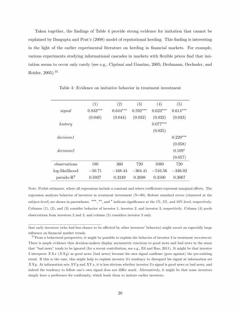
Taken together, the findings of Table 4 provide strong evidence for imitation that cannot be
explained by Dasgupta and Prat’s (2008) model of reputational herding. This finding is interesting
in the light of the earlier experimental literature on herding in financial markets. For example,
various experiments studying informational cascades in markets with flexible prices find that imi-
tation seems to occur only rarely (see e.g., Cipriani and Guarino, 2005; Drehmann, Oechssler, and
Roider, 2005).35
Table 4: Evidence on imitative behavior in treatment investment
(1) (2) (3) (4) (5)
signal 0.833∗∗∗ 0.644∗∗∗ 0.592∗∗∗ 0.623∗∗∗ 0.614∗∗∗
(0.040) (0.044) (0.032) (0.032) (0.033)
history 0.077∗∗∗
(0.025)
decision1 0.229∗∗∗
(0.058)
decision2 0.109∗
(0.057)
observations 180 360 720 1080 720
log-likelihood −50.71 −168.44 −364.41 −516.56 −346.02
pseudo-R2 0.5927 0.3249 0.2698 0.3100 0.3067
Note: Probit estimates, where all regressions include a constant and where coeffi cients represent marginal effects. The
regression analyzes behavior of investors in treatment investment (N=90). Robust standard errors (clustered at the
subject-level) are shown in parentheses. ∗∗∗, ∗∗, and ∗ indicate significance at the 1%, 5%, and 10% level, respectively.
Columns (1), (2), and (3) consider behavior of investor 1, investor 2, and investor 3, respectively. Column (4) pools
observations from investors 2 and 3, and column (5) considers investor 3 only.
that early investors (who had less chance to be affected by other investors’behavior) might excert an especially large
influence on financial market trends.35From a behavioral perspective, it might be possible to explain the behavior of investor 3 in treatment investment.
There is ample evidence that decision-makers display asymmetric reactions to good news and bad news in the sense
that “bad news”tends to be ignored (for a recent contribution, see e.g., Eil and Rao, 2011). It might be that investor
3 interprets XXx (XXy) as good news (bad news) because his own signal confirms (goes against) the pre-existing
trend. If this is the case, this might help to explain investor 3’s tendency to disregard his signal at information set
XXy. At information sets XY y and XY x, it is less obvious whether investor 3’s signal is good news or bad news, and
indeed the tendency to follow one’s own signal does not differ much. Alternatively, it might be that some investors
simply have a preference for conformity, which leads them to imitate earlier investors.
20
5.3 Wage setting by principals
Having documented imitative behavior on the part of investors, we now turn to the wage setting
of principals. Was their wage setting in line with theory? Did principals correctly anticipate the
actual behavior of investors in the experiment? And if yes, did the principals’wage setting behavior
lead to reduced incentives for reputational herding in treatment reputation?
Two benchmarks: equilibrium wages and behavioral wages To evaluate the actual wage
setting by principals in the experiment, we calculate two benchmark wages. The first benchmark are
the equilibrium wages req that are predicted by theory (see Proposition 2). As a second benchmark,
we calculate behavioral wages rbeh that would optimally have been set by profit-maximizing princi-
pals if they had correctly anticipated the actual behavior of investors in the experiment. In order
to calculate the behavioral wages rbeh, we proceed as follows. First, from the actual frequencies
with which the two types of investors 1, 2, and 3 follow their own signal in treatment reputation, we
calculate the empirical frequencies of facing a good investor (given a certain combination of history
of trades and realized value of the asset). Multiplying these empirical frequencies with the good
investor’s value of 20 points, we arrive at the behavioral wages rbeh.
Wage setting by principals relative to the benchmarks In a first step, we consider the
wages offered to investors 1 and 2. From a theoretical perspective, these investors always trade
sincerely, and the equilibrium wage req they receive depends on the success respectively failure of
the investment only (see Proposition 2). As illustrated in Table 5, on average, behavioral wages
offered to these investors would be less extreme than equilibrium wages. That is, behavioral wages
would be lower (higher) than equilibrium wages when the asset is successful (unsuccessful). Given
that the partially imitative behavior of investors makes it more diffi cult to gauge the investor’s type
from the outcome of the game, it does not seem surprising that behavioral wages would be closer
to 10 (which would be the optimal wage offer if one would not have any additional information
except for the prior probability of facing a good type). In order to evaluate actual wages setting, in
Table 5, we report rall (which is the average wage offer when considering all principals) and rmax
(where we only consider the maximum wages, i.e., the wages offered by winning principals). As
Table 5 documents, on average, rall is somewhat lower than the benchmarks req and rbeh, while
rmax overshoots both benchmarks. However, in line with the benchmark wages, rall and rmax
21

are significantly higher in case of success than in case of failure of the investment (according to
Wilcoxon-Signed-Ranks tests at the 1%-level and 5% level, respectively).36
Table 5: Average wages offered to investors 1 and 2
purchased asset is req rbeh rall rmax
unsuccessful 3.33 4.27 2.17 6.79
successful 12.86 11.83 10.34 16.15
In a second step, we consider wages offered to investor 3, which are displayed in Table 6.
When theory predicts herding, req is equal to 10 (because in this case the investor’s decision is
uninformative about his type). Otherwise, equilibrium wages only vary in the success or failure
of the investment. In line with both benchmark wages, principals seem to consider the history
of trades XXX as less informative of the respective investor’s type than other histories of trade
(because at histories of trade other than XXX wages are further away from 10).37 An interesting
observation with respect to behavioral wages emerges if the history of trades is given by XXX.
Then, the equilibrium prediction for the wage is 10 independent of the investment’s success. While
in case of a successful investment the behavioral wage rbeh is almost identical to this prediction,
in case of an unsuccessful investment rbeh is considerably lower. Hence, in contrast to what is
predicted by theory, even in these situations the failure of the investment seems to be predictive of
the investor’s type. More importantly, across the various settings considered in Table 6, for both
rall and rmax the relative ordering of the wages is identical to the relative ordering of rbeh: investor
3 fetches the lowest (highest) wage when the history of trade is not XXX and when his investment
is unsuccessful (successful). As in the case of the wages offered to investors 1 and 2, the wages rall
(rmax) that are offered to investor 3 somewhat undershoot (overshoot) the benchmark wage rbeh.
Nevertheless, principals’actual wage setting behavior comes relatively close to the benchmark rbeh.
36 In case of rall (rmax), we compare average wage offers for successful respectively unsuccessful investors at the
principal-level (at the session-level).37Only in case of an unsuccessful investment, the difference between wage bids rall given a history XXX and wage
bids rall given any other history is marginally statistically significant with p = 0.069 (Wilcoxon-Signed-Ranks test
that compares average wage bids at the principal-level).
22

Table 6: Average wages offered to investor 3
purchased asset is history of trades req rbeh rall rmax
unsuccessful = XXX 10.00 5.83 3.40 10.10
6= XXX 3.33 4.69 2.37 6.80
successful = XXX 10.00 10.01 9.42 16.10
6= XXX 12.86 11.30 10.31 16.53
Are there different behavioral types among the principals? One might suspect that prin-
cipals who themselves are prone to imitative behavior might set wages differently from other prin-
cipals. We investigate this issue by using data from treatment investment, where the principals
of treatment reputation acted as investors. We label a principal as an imitator if, in treatment
investment, he bought asset A at information set AAb and bought asset B at information set BBa.
This applies to 8 of the principals. The remaining 22 principals are labelled as non-imitators. In
order to study potential behavioral differences between these two types of principals, we focus on
the wages offered to investor 3. We do this to explore two issues: First, do different principals
react differently to investor 3 following his predecessors? And second, what role does the ultimate
success of investor 3’s decision play? While, due to large variances, differences are, in general,
not statistically significant, some suggestive patterns do emerge nonetheless (see Table 7, which
displays average wages rall).
Table 7: Average wages rall offered to investor 3 by imitators and non-imitators
purchased asset is
unsuccessful successful
history of trades non-imitators imitators non-imitators imitators
XXX 3.36 3.50 9.64 8.81
XXY 1.80 1.38 9.27 11.94
XY Y 2.86 3.31 10.18 9.94
XYX 2.25 3.00 11.18 9.81
Note: A principal is labelled an imitator if in treatment investment he bought asset A at information set AAb and
bought asset B at information set BBa, which applies to 8 (out of a total of 30) principals. All other principals are
labelled as non-imitators.
23

On average, principals offer higher wages to successful investors than to unsuccessful investors.
With one notable exception (to be discussed below), imitators tend to punish failure somewhat
less and reward success somewhat less than non-imitators do. That is, imitators seem to offer
slightly higher (lower) wages than non-imitators if the asset is unsuccessful (successful). This could
suggest that imitators perceive success (respectively failure) as less informative of the investor’s type
than non-imitators do. The interesting exception to this emerges if the history of trades is given
by XXY : if investor 3 decides to make an investment that contradicts both of his predecessors,
imitators seem to condition their wage offers on the success or failure of the investment decision
more strongly than non-imitators do. That is, imitators seem to deem acting against an established
trend as more informative about the respective investor’s type than non-imitators do. Moreover,
independent of the success of the investment, non-imitators reward herding (in the sense that they
make higher wage offers to investor 3 given a history of trades XXX than given a history of trades
XXY : 3.36 versus 1.80, and 9.64 versus 9.27). This is not the case for the imitators among the
principals (where in case of success of the investment, we have 8.81 versus 11.94).
Reputational incentives for investor 3 A key question is whether the actual wage setting
behavior of the principals in the experiment generates incentives for investor 3 to engage in rep-
utational herding. In order to investigate this issue, we look at each of the information sets that
investor 3 might face (i.e., XXy, XXx, XY x, and XY y). For each of these four cases, we derive
the difference between investor 3’s expected payoff when he does not follow his signal and investor
3’s expected payoff when he does follow his signal. We calculate these payoff differences under
various assumptions on what investor 3 believes about the behavior of investor 1, investor 2, and
the principals.
In column (1) of Table 8, we report the payoff differences predicted by Proposition 2. For this
case, column (1) indicates that investor 3 should engage in reputational herding at information set
XXy (yielding him a payoff that is 1.51 points higher than when trading sincerely). Investor 3
should follow his signal otherwise (as indicated by the negative payoff differences).38 In columns (2)
and (3) of Table 8, we assume that investor 3 holds the belief that investors 1 and 2 always act in line
with theory (i.e., always follow their signal). However, with respect to the wage offers, we assume
38Note that the history of trades XXY is off the equilibrium path. In order to calculate the respective payoff
difference, we assume that in this case principals hold the off-equilibrium belief that investor 3 has traded sincerely
(which is in line with the assumption made in Dasgupta and Prat, 2008).
24

that investor 3 correctly anticipates the actual wage setting behavior by principals: rall (column (2))
respectively rmax (column (3)). Interestingly, in both columns (2) and (3), reputational incentives
remain intact: an investor 3 holding such beliefs should still herd at information set XXy, but not
otherwise.
In columns (4) and (5) of Table 8, we assume that investor 3 not only correctly anticipates
actual wage setting by principals, but that he also correctly anticipates the actual behavior of
investors 1 and 2 in the experiment. That is, we assume that investor 3 anticipates the actual
frequencies with which investors 1 and 2 do not trade sincerely. In this case, given a certain history
of his predecessors’ decisions, investor 3 draws correct inference about the success probabilities
of the two assets. Columns (4) and (5) of Table 8 reveal that, if investor 3 held such correct
beliefs, reputational incentives to herd would disappear. This is so because not following the own
signal would always lead to a negative payoff. In column (6) of Table 8, we investigate whether
incentives for reputational herding would re-emerge if investor 3 held correct beliefs with respect
to the behavior of the other investors, and if, in addition, he expected optimal wage setting by
principals (i.e., wage offers rbeh). This is not the case because not following his own signal would
again always yield a negative payoff.
Table 8: Differences in expected payoffs of investor 3 from not following respectively following his
own signal under various beliefs on the behavior of investor 1, investor 2, and the principals
investor 3 assumes
sincere trading
by investors 1 and 2
investor 3 correctly
anticipates actual behavior
by investors 1 and 2
(1) (2) (3) (4) (5) (6)
information set req rall rmax rall rmax rbeh
XXy 1.51 0.45 0.85 -1.89 -0.38 -2.76
XXx -10.50 -8.93 -11.14 -7.14 -9.23 -3.30
XY x -7.81 -6.31 -6.81 -7.59 -8.12 -6.88
XY y -7.81 -6.14 -6.91 -5.68 -6.35 -4.75
To summarize, if we assume that investor 3 anticipates the actual (partly imitative) behavior
of earlier investors, then the monetary incentives for reputational herding disappear (see columns
(4)-(6) of Table 8). Hence, the apparent lack of reputational herding seems to be a consequence
of the noisy behavior of early investors who do not always follow their private signal. If earlier
25
decisions do not reveal the underlying private information, observing an established trend is less
indicative of the potential success of the investment. Hence, acting against the trend carries a
smaller loss in reputation than what theory would suggest (because acting against the trend does
less strongly suggest that the respective investor is a bad type). This smaller loss in reputation
might lead later investors to refrain from herding.
6 Conclusion
The possibility of herd behavior in financial markets has received considerable attention in both
the academic literature and the popular press. Various explanations have been put forward why
investors might tend to follow existing trends (e.g., social learning, reputational concern, or sim-
ply imitation). Purely information-based social-learning arguments have been studied extensively
in the theoretical and experimental literature. Reputational concerns of investors as a potential
source of herding have received relatively less attention. This seems somewhat surprising given
the prominence of reputation-based explanations among practitioners (see e.g., the introductory
quotation) and given the attention they have received in the empirical literature.
By now, there is a growing theoretical literature on reputational herding. To our knowledge, the
present paper is the first one to implement a theory of reputational herding in financial markets in
the laboratory. In particular, we consider the model by Dasgupta and Prat (2008), where investors
might disregard their private information and follow an existing trend because they worry about
later wage offers from an outside job market. Conducting an experiment allows to control for
the information that investors hold and for the incentives that they face. This is, in general, not
possible in an empirical study.
The intuition behind Dasgupta and Prat (2008) is as follows. They consider a sequential asset
market, where investors receive private information with respect to the prospects of two assets.
The precision of this signal depends on the investor’s unobservable ability type. Early investors
will find it optimal to trade sincerely, and, as a consequence, the market prices of the assets will
move closer towards their true values. Hence, profits from trading become smaller and smaller. At
the same time, for later investors, acting against an established trend comes at a cost because it
might leave the outside job market with the impression that the respective investor is a bad type
(who has received a wrong signal). Hence, the theory predicts that, depending on the history of
26

earlier trades, later investors might optimally disregard their private information and engage in
reputational herding.
Whether reputational herding indeed emerges depends on two things. First, whether investors
respond to the incentives set by the outside market, and second, whether the outside job market
indeed sets incentives for reputational herding. As a consequence, in the experiment, we consider
an explicit wage setting process where some of the subjects act as principals and make wage offers
to investors.
In the experiment, we find that it is indeed in the situations predicted by Dasgupta and Prat
(2008) that a substantial fraction of investors follows an established trend. However, this seems to
be driven by imitation rather than by reputational herding: a similar fraction of subjects engages
in such behavior even in a treatment where there is no outside job market (and where theory would
predict sincere trading by all investors). The fact that we document imitation that is not driven by
a profit motive seems to be interesting because such behavior has hardly been observed in earlier
experiments on herding in financial markets.
In the experiment, wages somewhat undershoot the theoretical prediction, while average winning
wages somewhat overshoot the theoretical prediction. To investigate the reputational incentives
investors have faced in the laboratory, we conduct a thought experiment. If we assume that investor
3 anticipates the actual (partly imitative) behavior of earlier investors, then the monetary incentives
for reputational herding disappear. Hence, the apparent lack of reputational herding might be
driven by the rather noisy behavior of early investors: Because early investors do not always follow
their private signal, observing an established trend is less indicative of the potential success of the
investment. Hence, acting against the trend carries a smaller loss in reputation than what theory
suggests (because acting against the trend does less strongly imply that the respective investor is
a bad type). This smaller loss in reputation might lead later investors to refrain from herding.
This raises the question whether, with a longer sequence of investors than considered in the
present experiment, incentives for reputational herding might re-emerge. In theory, this could
happen even when early investors’decisions do not perfectly reflect their private information: if
there is a suffi ciently long trend in the same direction, this might still provide suffi ciently precise
information on the true state of the world. However, suffi ciently long trends might not emerge:
While the settings are slightly different, experiments on social learning in financial market (see e.g.,
Cipriani and Guarino, 2005; Drehmann, Oechssler and Roider, 2005) have documented a strong
27

tendency of investors to engage in “contrarian behavior” (i.e., the higher the market price of an
asset, the less likely are investors to buy this asset). As a consequence, even with a longer sequence
of investors, asset prices might fail to become suffi ciently extreme for reputational concerns to
outweigh profits from trading according to one’s own information.
In our experiment, all investors were informed in the sense that each investor received a signal
that contained some information.39 That is, we abstract from completely uninformed investors. In
the real-world, in many stocks and markets, there will be substantial numbers of uninformed traders,
whose behavior is unlikely to be random. As a consequence, our present findings mainly apply to
stocks respectively markets in which uninformed traders play a limited role. As opposed to heavily
traded stocks, this may particularly hold for stocks that are diffi cult to assess or to arbitrage (see
e.g., Blasco and Ferreruela, 2008; Sias, 2004; Palomino, 1996). It would be an interesting, relevant
topic for future experimental research to study how the presence of uninformed traders affects
financial market outcomes.
References
Akerlof, G., and R. Shiller (2008): Animal Spirits: How Human Psychology Drives the Econ-
omy, and Why It Matters for Global Capitalism (New Edition). Princeton University Press.
Anderson, L., and C. Holt (1997): “Information Cascades in the Laboratory,”American Eco-
nomic Review, 87(5), 847—862.
Avery, C., and P. Zemsky (1998): “Multidimensional Uncertainty and Herd Behavior in Finan-
cial Markets,”American Economic Review, 88(4), 724—48.
Banerjee, A. (1992): “A Simple Model of Herd Behavior,” Quarterly Journal of Economics,
107(3), 797—817.
Bikhchandani, S., D. Hirshleifer, and I. Welch (1992): “A Theory of Fads, Fashion, Custom,
and Cultural Change as Informational Cascades,” Journal of Political Economy, 100(5), 992—
1026.39 In particular, this also holds for bad types because investors were assumed to be unaware of their type.
28
Bikhchandani, S., and S. Sharma (2000): “Herd Behavior in Financial Markets: A Review,”
IMF Policy Working Papers WP/00/48.
Blasco, N., and S. Ferreruela (2008): “Testing Intentional Herding in Familiar Stocks: An
Experiment in an International Context,”Journal of Behavioral Finance, 9(2), 72—84.
Chevalier, J., and G. Ellison (1999): “Career Concerns of Mutual Fund Managers,”Quarterly
Journal of Economics, 114(2), 389—432.
Cipriani, M., and A. Guarino (2005): “Herd Behavior in a Laboratory Financial Market,”
American Economic Review, pp. 1427—1443.
Daniel, K., D. Hirshleifer, and S. H. Teoh (2002): “Investor Psychology in Capital Markets:
Evidence and Policy Implications,”Journal of Monetary Economics, 49(1).
Dasgupta, A., and A. Prat (2006): “Financial Equilibrium with Career Concerns,”Theoretical
Economics, 1(1), 67—93.
(2008): “Information Aggregation in Financial Markets with Career Concerns,”Journal
of Economic Theory, 143(1), 83—113.
Dohmen, T., A. Falk, D. Huffman, U. Sunde, J. Schupp, and G. Wagner (2011): “Indi-
vidual Risk Attitudes: Measurement, Determinants, and Behavioral Consequences,”Journal of
the European Economic Association, 9(3), 522—550.
Drehmann, M., J. Oechssler, and A. Roider (2005): “Herding and Contrarian Behavior in
Financial Markets: An Internet Experiment,”American Economic Review, 95(5), 1403—1426.
Drehmann, M., J. Oechssler, and A. Roider (2007): “Herding With and Without Payoff
Externalities: An Internet Experiment,” International Journal of Industrial Organization, 25,
391—415.
Ehrbeck, T., and R. Waldmann (1996): “Why are Professional Forecasters Biased? Agency
Versus Behavioral Explanations,”Quarterly Journal of Economics, 111(1), 21—40.
Eil, D., and J. M. Rao (2011): “The Good News—Bad News Effect: Asymmetric Processing
of Objective Information about Yourself,”American Economic Journal: Microeconomics, 3(2),
114—138.
29

Glosten, L., and P. Milgrom (1985): “Bid, Ask and Transaction Prices in a Specialist Market
with Heterogeneously Informed Traders,”Journal of Financial Economics, 14(1), 71—100.
Graham, J. (1999): “Herding Among Investment Newsletters: Theory and Evidence,”Journal of
Finance, 54(1), 237—268.
Greiner, B. (2004): “An Online Recruitment System for Economic Experiments,” in Forschung
und Wissenschaftliches Rechnen 2003, ed. by K. Kremer, and V. Macho, pp. 79—93. GWDG
Bericht 63. Gesellschaft für Wissenschaftliche Datenverarbeitung, Göttingen.
Hirshleifer, D., and S. H. Teoh (2003): “Herd Behavior and Cascading in Capital Markets: A
Review and Synthesis,”European Financial Management, 9(1), 25—66.
Holmstrom, B. (1999): “Managerial Incentive Problems: A Dynamic Perspective,” Review of
Economic Studies, 66(1), 169—182.
Hong, H., and J. Kubik (2003): “Analyzing the Analysts: Career Concerns and Biased Earnings
Forecasts,”Journal of Finance, 58(1), 313—351.
Hong, H., J. Kubik, and A. Solomon (2000): “Security Analysts’Career Concerns and Herding
of Earnings Forecasts,”Rand Journal of Economics, pp. 121—144.
Huddart, S. (1999): “Reputation and Performance Fee Effects on Portfolio Choice by Investment
Advisers,”Journal of Financial Markets, 2(3), 227—271.
Irlenbusch, B., and D. Sliwka (2006): “Career Concerns in a Simple Experimental Labour
Market,”European Economic Review, 50(1), 147—170.
Koch, A., A. Morgenstern, and P. Raab (2009): “Career Concerns Incentives: An Experi-
mental Test,”Journal of Economic Behavior & Organization, 72(1), 571—588.
Lamont, O. (2002): “Macroeconomic Forecasts and Microeconomic Forecasters,”Journal of Eco-
nomic Behavior & Organization, 48(3), 265—280.
Massa, M., and R. Patgiri (2007): “Compensation and Managerial Herding: Evidence from the
Mutual Fund Industry,”mimeo.
Palomino, F. (1996): “Noise Trading in Small Markets,”Journal of Finance, 51(4), 1537—1550.
30

Park, A., and H. Sabourian (2011): “Herding and Contrarian Behavior in Financial Markets,”
Econometrica, 79(4), 973—1026.
Park, A., and D. Sgroi (2010): “Herding and Contrarian Behavior in Financial Markets: An
Experimental Analysis,”mimeo.
Scharfstein, D., and J. Stein (1990): “Herd Behavior and Investment,”American Economic
Review, 80(3), 465—79.
Sias, R. (2004): “Institutional Herding,”Review of Financial Studies, 17(1), 165—206.
Villatoro, F. (2009): “The Delegated Portfolio Management Problem: Reputation and Herding,”
Journal of Banking & Finance, 33(11), 2062—2069.
Weizsacker, G. (2010): “Do We Follow Others When We Should? A Simple Test of Rational
Expectations,”American Economic Review, 100, 2340—2360.
Welch, I. (1992): “Sequential Sales, Learning, and Cascades,”Journal of Finance, 47(2), 695—732.
(2000): “Herding Among Security Analysts,” Journal of Financial Economics, 58(3),
369—396.
31

Appendix
A Wages and investment in the presence of reputational concerns
In this appendix, we illustrate how, building on Dasgupta and Prat’s (2008) Proposition 4, the wage
bids and investment behaviors as spelt out in Proposition 2 can be derived (given the parameter
values we have assumed). In particular, we show that these wage bids and investment behaviors
are mutually best replies.40
Wage bids First, suppose an investor’s equilibrium strategy tells him to invest sincerely (which
will be the case for investors 1 and 2, and investor 3 unless both of his predecessors have chosen
the same asset). In this case, as outlined in Section 3.3, the equilibrium wage bids for this investor
depend on the ultimate success (respectively failure) of his investment only (i.e., whether V i = v or
V i 6= v holds). In particular, the potential wage bids r(V i = v) and r(V i 6= v) equal the conditional
probabilities of facing a good type times the good type’s value of 20, where
r(V i = v) =
[σg
0.5σb + 0.5σg· 1
2
]· 20 = 12.86 and (4)
r(V i 6= v) =
[1− σg
1− 0.5σb − 0.5σg· 1
2
]· 20 = 3.33. (5)
Hence, r(V i = v) > r(V i 6= v), i.e., success of the investment is more indicative for a good type.
Second, suppose investors 1 and 2 have chosen the same asset and investor 3’s strategy tells
him to herd in this case. Then, investor 3’s trade does not reveal any information about his type.
Independent of the success of his investment, he will receive wage offers that are determined by the
prior probability of being a good type and given by 12 · 20 = 10.41
Investment behavior We now turn to the behavior of investors and take the wage offers as spelt
out in Proposition 2 as given. Given a certain realization of his signal, an investor will compare
his expected payoff from trading sincerely with his expected payoff from trading against his signal.
Denote this payoff difference by ∆πR = ∆πI + ∆r, where ∆πI denotes the expected difference in
40Note that while, in principle, the most-revealing equilibrium may be in mixed strategies, this is not the case given
the parameter values assumed here.41Note that, in line with Dasgupta and Prat (2008), we assume that if investor 3 would deviate and not herd this
would imply an off-equilibrium belief of a sincere trade.
1

the profits from trading per se, where ∆r denotes the expected difference in wages, and where,
for ease of exposition, the arguments of the functions are omitted. The respective investor trades
sincerely whenever ∆πR > 0 holds (see (3)).
Table 9 displays ∆r, ∆πI , and ∆πR for all information sets of the game. In order to illustrate
how the entries of Table 9 are calculated, suppose that investor i has received signal si = a and
faces history Ht (recall that investor i buys at time t = i only). In this case, we have
∆r = Pr(v = A|a,Ht) ·[r(v = V i = A)− r(v 6= V i = B)
]+
Pr(v = B|a,Ht) ·[r(v 6= V i = A)− r(v = V i = B)
].
(6)
For example, suppose it is investor 3 who has received an a-signal and, in addition, both predecessors
buy asset B. In this case, investor 3 would update to an probability of 0.7 of asset A being the
unsuccessful one. Not trading sincerely (V i = B) would reveal no information about investor 3’s
type to the principal (as this would be in line with the candidate equilibrium strategy), and as a
consequence investor 3 receives a wage of 10. In contrast, if investor 3 would deviate and purchase
asset A, the principals would hold an off-equilibrium belief of sincere trading and, depending on the
success of the investment, offer a wage of either 12.86 or 3.33. As a consequence, in this case, (6)
would imply ∆r = 310(12.86−10)+ 7
10(3.33−10) = −3.81. At the same time, in the present case, we
have ∆πI = 9.3−7.0 = 2.3: while the expected payoff from trading sincerely is zero, when following
the herd investor 3 has to pay a market price of 9.3 for assetB, which according to the information he
holds has an expected value of 7 only (see Table 1). Hence, ∆πR = ∆πI +∆r = 2.3−3.81 = −1.51,
and investor 3 should optimally herd in this case.42
All remaining values of ∆r, ∆πI , and ∆πR are derived in a completely analogous way.
42As discussed in Section 3.3, the asset prices presented to subjects are calculated under the assumption that trade
is sincere in both treatments. If, in line with Dasgupta and Prat (2008), the market maker would anticipate herding
by investor 3 and set asset prices accordingly, in the present case one would have ∆πI = 1.4 and ∆πR = −2.41.
Hence, the same theoretical prediction would emerge.
2
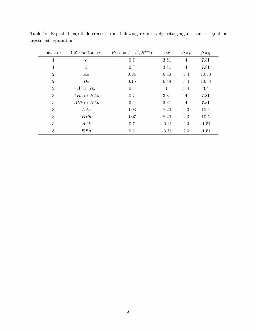
Table 9: Expected payoff differences from following respectively acting against one’s signal in
treatment reputation
investor information set Pr(v = A | si, Ht=i) ∆r ∆πI ∆πR
1 a 0.7 3.81 4 7.81
1 b 0.3 3.81 4 7.81
2 Aa 0.84 6.48 3.4 10.88
2 Bb 0.16 6.48 3.4 10.88
2 Ab or Ba 0.5 0 3.4 3.4
3 ABa or BAa 0.7 3.81 4 7.81
3 ABb or BAb 0.3 3.81 4 7.81
3 AAa 0.93 8.20 2.3 10.5
3 BBb 0.07 8.20 2.3 10.5
3 AAb 0.7 -3.81 2.3 -1.51
3 BBa 0.3 -3.81 2.3 -1.51
3

B Experimental instructions: English translation
As discussed in Section 4, both rounds of a session had the same basic structure. The instruc-
tions for the respective round were handed to subjects and read out aloud by the experimenter.
In addition, the main features of the respective round were explained via a flip chart to subjects.
Decision sheets for the respective round were only distributed after all subjects had correctly com-
pleted a questionnaire about details of the experimental setup. In the second round, investors and
observers faced slightly different questions, where the wording was adjusted to take account of the
different roles of the participants. The below instructions contain the second-round questionnaire
that principals had to complete. Participants were given the opportunity to record their first round
decisions on a separate sheet of paper, to which they had access in the second round of the experi-
ment. Importantly, we made it clear to subjects that second-round decision-making did not require
recalling first-round decisions. Only after the second round, payments were calculated, subjects
answered a post-experimental questionnaire requesting demographic information as well as asking
questions about the experiment. Finally, payments were privately handed out to subjects, after
which the experiment ended.
All phrases emphasized in the subsequent translation were also emphasized in the original
instructions. Square brackets contain explanations intended for the reader and were not part of the
original instructions.
Instructions
Welcome
Welcome to our experiment. The laboratory for experimental economics - AWI Lab - at the
Department of Economics of the University of Heidelberg (game administrator: Professor Roider)
aims to test various scientific theories with this experiment.
Payment
By participating in the experiment, you support our scientific work. You are guaranteed to receive 4
Euros. At the same time, you may earn additional money through your decisions in the experiment.
A more detailed explanation of how your payment is calculated will be provided later. Each Point
1

earned in our experiment corresponds to 0.20 Euro. The experiment will take approximately 120
minutes.
The Experiment
The experiment consists of two rounds that are completely independent of each other. In each
round the players are randomly assigned to groups (which will change from round to round),
and players will have to take investment decisions. To aid you in your decision, you will receive
information about the potential success of various investments and you will learn the decisions of
your predecessors in your group.
Now, on to the game!
[Start of instructions for Round 1]
Round 1
The investment decision
Each group consists of three investors, who sequentially make investment decisions. Each investor
must choose between two shares (A and B). Only one share will turn out to be successful and
have a value of 10 Points at the end. The other share will turn out to be worthless and have a
value of 0 Points. Which share is successful, is determined randomly before the first investor of the
respective group makes his decision. Hence, the same share is successful for all investors in your
group. Without additional information you can rely on the fact that in 50% of cases share A
is successful and in 50% of cases share B is successful.
Additional Information
Each investor can observe the investment decisions of his predecessors in his group.
Moreover, prior to making his decision, every investor receives an additional tip about whether
share A or B is successful. The reliability of the tip depends on which of two possible sources
of information the investor can draw on: a good source of information or a bad source of
information. Which of the two sources of information is available to a given investor is deter-
mined randomly, and may differ across investors even within a given group. For each investor, the
2

probability of drawing on a good source of information is the same and equal to 50%. Likewise, for
each investor, the probability of drawing on a bad source of information is 50%.
Each investor knows neither the quality of his source of information nor the quality of the source
of information any other investor is drawing on.
Bad source of information: Investors who “draw on a bad source of information”are privately
shown a ball that is randomly drawn from an urn containing 5 “A-Balls”and 5 “B-Balls.”For each
of these investors, a new ball is drawn from this 5:5 urn (where the respective ball is returned to
the urn after it has been shown to the respective investor). Consequently, these investors might
be receiving different tips.
Good source of information: Investors who “draw on a good source of information”are privately
shown a ball that is randomly drawn from an urn where the number of “A-Balls”and “B-Balls”in
the urn depends on which asset is successful. If asset A is successful, the urn contains 9 “A-Balls”
and 1 “B-Ball.”If, however, asset B is successful, the urn contains 9 “B-Balls”and 1 “A-Ball.”For
each of the investors who can draw on a good source of information a new ball is drawn from this
9:1 urn (where the respective ball is returned to the urn after it has been shown to the respective
investor). Consequently, these investors might be receiving different tips too.
Each investor knows his own tip only and does not observe the tips other investors have received.
Summary: Each investor in your group faces the same problem as you do. He has to choose
between share A and share B. Each investor receives a tip in form of an “A-Ball”or a “B-Ball”,
which only he can observe. Each investor knows neither the quality of his source of information nor
the quality of the source of information any other investor is drawing on. However, prior to making
his decision, each investor can observe the decisions of his predecessors in his group (if applicable),
and he can observe the prices (and history of prices) of the shares.
Prices
Each investor who decides on buying a certain share has to pay the current share price. The current
price of a given share is adjusted upwards or downwards on the basis of the observed investment
decisions by the experimenter.
3

Each investor receives an endowment of 20 Points for Round 1 of the experiment.
We elicit your decision for every possible scenario
In the following, we will ask for your decision for every possible scenario that may occur.
In particular, you will be asked to put yourself in the shoes of investor 1 and to make a decision
for the case that you are shown an “A-Ball”as well as for the case that you are shown a “B-Ball”.
Subsequently, you will be asked to put yourself in the shoes of investor 2 and to make a decision
for every possible combination of investor 1’s decision and tip that you might receive.
Finally, you will be asked to put yourself in the shoes of investor 3 and to again make decisions for
every possible scenario.
Calculation of your payment
How do we calculate the payment that you receive at the end of the experiment? Once the
experiment has ended and after all investment decisions have been made, for each group the
experimenter will randomly determine who occupies the role of investor 1, investor 2, and investor
3. Subsequently, for each group there will be random draws (according to the rules described above)
that determine (a) which share is the successful one, (b) from which urn the tip for the respective
investor is picked, and (c) the tip that the respective investor is shown.
As an example, suppose that you have been assigned the role of investor 1, and an “A-Ball”has
been drawn for investor 1. In this case, the decision you made for investor 1 given that he is shown
an “A-Ball”would determine your payment.
Now, suppose that you have been assigned the role of investor 2. Furthermore, suppose that your
group’s investor 1 has bought share B (given the random draws specified above), and an “A-Ball”
has been drawn for investor 2. In this case, the decision you made for Investor 2 in the scenario
(Investor 1 bought B, your tip: “A-Ball”) would determine your payment.
Completely analogous, if you have been assigned the role of investor 3, your payment is determined
by the decision you made in the relevant scenario (i.e., given your predecessors’decisions and own
tip that are selected according to the rules just described).
4

Hence, by the above procedure, one of your decisions is selected and determines your payment.
The number of Points that results from this decision depends on the true value of the share you
have bought and the share price you have paid. In any case, the share price you have paid is
deducted from your endowment. This will be your payment for the current round if your share is
not the successful one. If, on the other hand, the share you have bought is successful, you receive
10 additional Points. Hence, one of the decisions you have made in this round determines your
payment.
The composition of groups will remain anonymous. You will not learn the identity of your fellow
investors.
Have you understood everything?
Before you continue, please answer the following questions so that we can ensure that you have
understood everything:
1. Before you observe a ball: What is the probability that share A is the successful one?
• 50%
• 90%
2. Suppose that you have access to the good source of information. What is the probability that
you observe a ball that represents the correct share?
• 50%
• 90%
3. What is the probability that you observe a ball from the good source of information?
• 50%
• 90%
4. What kind of information does investor 1 receive before he takes his decision?
• His tip in form of a ball and the share prices
5

• His tip in form of a ball and the quality of his source of information
• His tip in form of a ball, the quality of his source of information, and which of the shares
has a value of 10
5. What kind of information does investor 2 receive before he takes his decision?
• His tip in form of a ball, and current and past share prices
• His tip in form of a ball and the quality of his source of information
• His tip in form of a ball, current and past share prices, and the decision of investor 1
• His tip in form of a ball, the quality of his source of information, and which of the shares
has a value of 10
6. What kind of information does investor 3 receive before he takes his decision?
• His tip in form of a ball, the quality of his source of information, and which of the shares
has a value of 10
• His tip in form of a ball and the quality of his source of information
• His tip in form of a ball, and current and past share prices
• His tip in form of a ball, current and past share prices, and the decisions made by
investors 1 and 2
7. Suppose that investor 1 observes an “A-Ball”as a tip. What tip will investor 2 receive?
• Investor 2 will also observe an “A-Ball”
• A new ball is drawn for investor 2
8. Suppose that both investor 1 and investor 2 receive an “A-Ball” as a tip. What tip will
investor 3 receive?
• Investor 3 will also observe an “A-Ball”
• A new ball is drawn for investor 3
6

9. Suppose that you have bought share A and that share A has a value of 10 Points. The
purchase price amounts to 7 Points. Your endowment is 20 Points. What is your payment
for this round?
• 10-7=3
• 20+7-10=17
• 20+10-7=23
• 20-7=13
10. Suppose that you have bought share A and that share A has a value of 0 Points. The purchase
price amounts to 4 Points. Your endowment is 20 Points. What is your payment for this
round?
• 20-4=16
• 20+10-4=26
• -4
• 10-4=6
[Participants have to answer all questions. Answers are checked. Only after all participants answer
all questions correctly, the following decision sheets are distributed.]
Scenarios in Round 1
Your Task
Put yourself in investor 1’s shoes:
Suppose you receive a certain ball as a tip, and subsequently you have to decide whether to buy
share A or share B at the indicated price. Bold print indicates the price you have to pay for share
A respectively share B. Now, for each of the scenarios described below, please state whether you
want to buy share A or share B:
7

Scenario 1
Price of share A 7,0
Price of share B 7,0
You receive an A-Ball. I buy: o share A o share B
Scenario 2
Price of share A 7,0
Price of share B 7,0
You receive an B-Ball. I buy: o share A o share B
Now, put yourself in investor 2’s shoes:
Suppose you observe both investor 1’s decision and the movement of share prices. In addition, you
receive a certain ball as a tip. Now, for each of the scenarios described below, please state whether
you want to buy share A or share B at the indicated price (in bold print). That is, the price in
bold print is the price you have to pay for share A respectively share B. The prices to the left are
the prices that your respective predecessors had to pay.
Scenario 1
Investor 1 2
Price of share A 7,0 8,4
Price of share B 7,0 5,0
Decision A ?
You receive an A-Ball. I buy: o share A o share B
Scenario 2
Investor 1 2
Price of share A 7,0 5,0
Price of share B 7,0 8,4
Decision B ?
You receive an A-Ball. I buy: o share A o share B
[The structure of the remaining two Scenarios that investor 2 may face is completely analogous,
and therefore these Scenarios are omitted from this translation of the experimental instructions.]
Now, put yourself in investor 3’s shoes:
Suppose you observe the investment decisions of the first two investors and the movement of share
prices. In addition, you receive a certain ball as a tip. Now, for each of the scenarios described
8

below, please state whether you want to buy share A or share B at the indicated price (in bold
print). That is, the price in bold print is the price you have to pay for share A respectively share
B. The prices to the left are the prices that your respective predecessors had to pay.
Scenario 1
Investor 1 2 3
Price of share A 7,0 8,4 7,0
Price of share B 7,0 5,0 7,0
Decision A B ?
You receive an A-Ball. I buy: o share A o share B
Scenario 2
Investor 1 2 3
Price of share A 7,0 8,4 7,0
Price of share B 7,0 5,0 7,0
Decision A B ?
You receive an B-Ball. I buy: o share A o share B
[The structure of the remaining six Scenarios that investor 3 may face is completely analogous, and
therefore these Scenarios are omitted from this translation of the experimental instructions.]
[End of instructions for Round 1 and start of instructions for Round 2]
Round 2
In Round 2, for investors the rules of the game are the same as in Round 1; only the calculation
of the compensation differs, and, in addition to investors, there will now also be observers. If you
have just drawn a card with an “I”, you are still an investor. If you have just drawn a card with
a “B”, you now act as an observer. Thereby, out of all Round 1 investors, we have anonymously
and randomly selected 6 participants, who now assume the role of observers.
Observers do not invest, but evaluate the investment decisions made by the investors. The observers
are not part of any investor group. The identity of both investors and observers will not be revealed.
Except for how their compensation is calculated, nothing changes for investors.
9

Calculation of your payment
This stays the same:
As in Round 1, we will ask for your decision for every possible scenario that may occur.
Again, each investor and each observer receives an endowment of 20 Points for Round 2.
After the experiment, i.e., after all investors and observers have made their decisions, the exper-
imenter will again randomly allocate investors to groups. That is, in Round 2 each investor has
different group members than in Round 1. Again, the roles of investor 1, investor 2, and investor
3 will be assigned randomly. Again, for each group in Round 2 there will be random draws (ac-
cording to the rules described above) that determine (a) which share is the successful one, (b) from
which urn the tip for the respective investor is picked, and (c) the tip that the respective investor
is shown.
Hence, by the above procedure, the decision that determines the payment is selected. That is, as
before, one of the decisions an investor makes in this Round will determine his/her payment.
This changes:
The true values of the shares continue to affect the investors’compensation. However, the observers’
compensation does not depend on the true values of the shares.
The additional compensation that an investor receives depends on the evaluation by the observers.
In particular, the observers do no longer decide between the two shares. Instead, observers now
have to estimate with which probability an investor had access to a good sources of information
when making his investment decision, and they will offer wages to individual investors.
Observers are willing to offer a wage because, by employing an investor with a good source of
information, they can earn Points. If an observer hires an investor who has access to a good source
of information, employing the investor is helpful and the observer receives additional 20 Points. An
observer does not benefit from hiring an investor with a bad source of information. In this case,
the observer receives no additional Points.
10

For each possible scenario and each investor, the 6 observers have to submit wage offers between
0 and a maximum of 20 Points (which they would be willing to pay for the respective investor).
The observer submitting the highest of the 6 wage offers for a given investor (in a given scenario)
hires the respective investor and pays the investor the wage offer he has made. The remaining 5
observers (who did not submit the highest wage offer) do not receive additional Points, but also do
not have to pay any wage. Now, there are 4 investor groups with a total of 12 investors.
The observers submit their wage offers at a point in time when the true values of the shares can
already be observed. On top of that, the observers can only observe the investment decisions of the
individual investors and the movement of share prices. They do not observe the tips that investors
have received, and they do not observe the qualities of investors’sources of information.
Sequence of events
As in Round 1, after all investors and observers have made their decisions for all possible scenarios,
for each group the decisions that determine the compensation and the true values of the shares are
determined.
The wage offers of the 6 observers for a given investor in the thus determined setting are compared,
and the highest bidding observer wins the respective bid. Thereby, for each investor in each group,
both the wage and which observer pays this wage are determined.
It is important to remember that observers do not learn investors’tips and source of information.
Observers only observe the investment decisions, the true values of the shares, and the movement
of share prices.
The Points you will receive are calculated as follows:
Payment to observers
If an observer has submitted the highest bid for a given investor, he pays his bid as a wage to
the respective investor. If the respective investor has a good source of information, the observer
receives an additional 20 Points. If multiple observers submit the same (highest) bid for a particular
investor, the winning bidder is determined randomly. Observer who have not submitted the highest
bid do not have to pay a wage and do not receive any additional Points.
11

Consequently, a given observer may submit the winning bid for none, one, multiple, or even all 12
of the investor(s). Please note: If an observer would incur an overall loss, he will earn 0 Points for
this round.
Hence, observers’decisions affect both their own as well as investors’compensation.
Payment to investors
An investor’s total compensation is determined by his initial endowment, the true value of the share
he has bought minus the share price he has paid, and the wage received from one of the observers.
[The below version of the questionnaire had to be completed by observers. Investors faced slightly
different questions, where the wording was adjusted to take account of the different role of the
subject.]
Have you understood everything?
Before you continue, please answer the following questions so that we can ensure that you have
understood everything:
1. Suppose that you have submitted a wage offer of 9 Points and won the bid. The investor
whom you are, hence, employing has bought share A, and share A has a true value of 10
Points. The investor has an initial endowment of 20 Points and has bought share A for a
price of 6 Points. Moreover, the investor has a good source of information.
(a) What is the investor’s total compensation in the current round?
• 9+10-6+20+20=53
• 9+20=29
• 9+10-6+20=33
(b) What is your payoff from employing this investor (excluding your initial endowment)?
• 20-9=11
• 20+10+9-6=33
12

• 9+20=29
(c) What would your compensation have been if the investor had had a bad source of
information and you had won the bid (excluding your initial endowment)?
• 0-9=-9
• 20+10+9-6+0=33
• 9+0=9
(d) Now, suppose that the share has a true value of 0 Points. What is the investor’s total
compensation?
• 9+0-6+20+20=43
• 9+20=29
• 9+0-6+20=23
2. You and one other observer have bid 14 Points for an investor. Who wins?
• Both of the observers win the bid. The profit is shared equally.
• The winner is selected randomly
• None of the observers wins the bid
3. To what kind of information do you have access when deciding on your wage offer?
• The investors’sources of information and the true values of the shares
• The tips the investors have received and the true values of the shares
• The investors’decisions and the movement of prices
• The investors’decisions, the movement of prices, and the true values of the shares
[Participants have to answer all questions. Answers are checked. Only after all participants answer
all questions correctly, decision sheets are distributed. Investors and observers are handed different
decision sheets, where each group only observes its own decision sheet.]
Scenarios in Round 2 [decision sheet of investors]
13

Please note: Round 2 and Round 1 are independent of each other.
[The remainder of the Round 2 decision sheet of investors is identical to the Round 1 decision sheet
displayed above, and it is therefore omitted from this translation of the experimental instructions.]
Scenarios in Round 2 [decision sheet of observers]
Your Task:
Below, we display all scenarios that may occur. For each scenario, please indicate what wage offer
between 0 and 20 you want to make for investor 1, investor 2, and investor 3, respectively.
In each case, you can observe the movement of prices, the prices each investor faced, which share
each investor bought, and which of the shares turned out to be successful.
Scenario 1
Investor 1 2 3
Price of share A 7,0 8,4 7,0
Price of share B 7,0 5,0 7,0
Decision A B A Successful share: A
Your wage offer for Investor 1:
Your wage offer for Investor 2:
Your wage offer for Investor 3:
[The structure of Scenarios 2 through 15 that an observer may face is completely analogous, and
therefore these Scenarios are omitted from this translation of the experimental instructions.]
Scenario 16
Investor 1 2 3
Price of share A 7,0 5,0 3,0
Price of share B 7,0 8,4 9,3
Decision B B B Successful share: B
Your wage offer for Investor 1:
Your wage offer for Investor 2:
Your wage offer for Investor 3:
14

[After subjects hand in their Round 2 decision sheets they answer the following post-experimental
questionnaire.]
Personal Data and Questionnaire
Thank you for participating in the experiment. We will now calculate your total Points, convert it
into Euros, and then hand you your payment. This may take a few minutes. In the meantime, we
would like to ask you to complete the following questionnaire.
Please do not talk to other participants and please refrain from using your cell phone until the end
of the experiment.
As soon as we have determined your payoff, we will call your number.
Thank you again for your participation!
Personal Data
Please answer the following questions. Of course, the results of the experiment will be anonymized,
and it will not be possible to connect the results to your personal data. The information you share
with us will be used for scientific purposes only.
[Data entry fields for age, gender, student status, Ph.D. status, field of studies, year of studies.]
Questionnaire
We would like to ask you to answer the following questions.
1. What would you do in the following situation: Suppose you have just won 100,000 Euros in
a lottery. Immediately after receiving this money, you are offered the following lottery:
There is a chance to double your money, but, at the same time, it is equally possible that
you could lose half of the amount you invested.
You can wager your entire 100,000 Euros, a fraction thereof, or you can choose not to take
part in this lottery at all.
What fraction of your winnings do you want to wager on this risky, but potentially profitable
lottery?
15

• the entire 100,000 Euros
• 80,000 Euros
• 60,000 Euros
• 40,000 Euros
• 20,000 Euros
• Nothing, I would not take part in this lottery
2. Do you think that investor 1 always has decided as suggested by the tip he has received?
3. Do you think that investor 2 always has decided as suggested by the tip he has received? If
not: When did he not act in line with his tip?
4. Do you think that investor 3 always has decided as suggested by the tip he has received? If
not: When did he not act in line with his tip?
5. When acting as an investor, did you base your decisions on the tips you received or on the
other investors’decisions?
6. What do you think was the purpose of this experiment?
7. In your daily decision-making, are you inclined to follow
• other people’s advice
• your own assessment
• other people’s advice in some situations and my own assessment in others
Thank you for filling out the questionnaire and for taking part in the experiment.
Please wait until your number is called.
16

C Example for how individual payoffs were calculated in the ex-
periment
In the following, we provide an example of how subjects’ payoffs were calculated in treatment
reputation. In each session of treatment reputation, 6 randomly selected subjects acted as principals,
while the remaining 12 subjects acted as investors. For the sake of the example, denote the 12
subjects who acted as investors by Sj for j = 1, ..., 12. As discussed in Section 4, after all subjects
had handed in their decision sheets, individual payoffs of subjects were calculated in the following
way. In a step (i), the 12 investors are randomly allocated into 4 groups of 3 investors each, and the
roles of investors 1, 2, and 3 are randomly assigned. Suppose that this random draw leads to one
of these groups being comprised of S2, S5, and S4, who act as investors 1, 2, and 3, respectively.
Furthermore, suppose that (as described in Section 4) in the random draws of step (ii), it turns
out that asset A is the successful one, S2 is a good type and receives signal a, S5 is a good type
and receives signal b, and S4 is a bad type and receives signal b. Then, from the decision sheet
of S2 (see Appendix B), we look up S2’s decision given that he plays investor 1 and has received
signal a. Let’s say S2’s decision is to buy A. Subsequently, we turn to S5’s decision sheet (who in
the current example acts as investor 2). There, we look up his decision given that investor 1 has
chosen A and S5 has received signal b. Let’s say S5’s decision is to buy B. Lastly, we turn to S4’s
decision sheet (who in the current example acts as investor 3). There, we look up his decision given
that investor 1 has chosen A, investor 2 has chosen B, and S4 has received signal b. Let’s say S4’s
decision is to buy A. Thereby, we have determined the payoff-relevant decisions of S2, S5, and S4
(which are given by A, B, and A, respectively). Moreover, given that in the present example asset
A is the successful one, we can now calculate each investor’s payoff that he obtains from buying the
respective asset (where it turns out that S2 and S4 bought the successful asset A, while S5 bought
the unsuccessful asset B).
To determine the wages of S2, S5, and S4, we proceed in the following way. In the decision sheets
of the six principals we look up the principals’wage offers for investor 1, investor 2, and investor
3 given a history of decisions H4 ∈ {ABA} and given that A is the successful asset (see “Scenario
1” in the decision sheet of principals in Appendix B). S2 (who, in the present example, acted as
investor 1) will then receive as a wage the highest offer made for investor 1, and the respective
highest-bidding principal gets a payoff from employing S2 (i.e., 20 minus the wage, because, in the
1

present example, S2 is a good type). Likewise, S5 (who, in the present example, acted as investor 2)
will then receive as a wage the highest offer made for investor 2, and the respective highest-bidding
principal gets a payoff from employing S5 (i.e., 20 minus the wage, because, in the present example,
S5 is a good type). Finally, S4 (who, in the present example, acted as investor 3) will then receive
as a wage the highest offer made for investor 3, and the respective highest-bidding principal gets
a payoff from employing S4 (i.e., 0 minus the wage, because, in the present example, S4 is a bad
type).
2