econstorMake Your Publications Visible.

A Service of

zbwLeibniz-InformationszentrumWirtschaftLeibniz Information Centrefor Economics

Prat, Julien; Walter, Benjamin

Working Paper

An Equilibrium Model of the Market for Bitcoin Mining

CESifo Working Paper, No. 6865

Provided in Cooperation with:Ifo Institute – Leibniz Institute for Economic Research at the University of Munich

Suggested Citation: Prat, Julien; Walter, Benjamin (2018) : An Equilibrium Model of the Marketfor Bitcoin Mining, CESifo Working Paper, No. 6865, Center for Economic Studies and ifoInstitute (CESifo), Munich

This Version is available at:http://hdl.handle.net/10419/174988

Standard-Nutzungsbedingungen:

Die Dokumente auf EconStor dürfen zu eigenen wissenschaftlichenZwecken und zum Privatgebrauch gespeichert und kopiert werden.

Sie dürfen die Dokumente nicht für öffentliche oder kommerzielleZwecke vervielfältigen, öffentlich ausstellen, öffentlich zugänglichmachen, vertreiben oder anderweitig nutzen.

Sofern die Verfasser die Dokumente unter Open-Content-Lizenzen(insbesondere CC-Lizenzen) zur Verfügung gestellt haben sollten,gelten abweichend von diesen Nutzungsbedingungen die in der dortgenannten Lizenz gewährten Nutzungsrechte.

Terms of use:

Documents in EconStor may be saved and copied for yourpersonal and scholarly purposes.

You are not to copy documents for public or commercialpurposes, to exhibit the documents publicly, to make thempublicly available on the internet, or to distribute or otherwiseuse the documents in public.

If the documents have been made available under an OpenContent Licence (especially Creative Commons Licences), youmay exercise further usage rights as specified in the indicatedlicence.

www.econstor.eu

6865 2018

January 2018

An Equilibrium Model of the Market for Bitcoin Mining Julien Prat, Benjamin Walter

Impressum:  

CESifo Working Papers ISSN 2364‐1428 (electronic version) Publisher and distributor: Munich Society for the Promotion of Economic Research ‐ CESifo GmbH The international platform of Ludwigs‐Maximilians University’s Center for Economic Studies and the ifo Institute Poschingerstr. 5, 81679 Munich, Germany Telephone +49 (0)89 2180‐2740, Telefax +49 (0)89 2180‐17845, email office@cesifo.de Editors: Clemens Fuest, Oliver Falck, Jasmin Gröschl www.cesifo‐group.org/wp   An electronic version of the paper may be downloaded  ∙ from the SSRN website:           www.SSRN.com ∙ from the RePEc website:          www.RePEc.org ∙ from the CESifo website:         www.CESifo‐group.org/wp    

 

CESifo Working Paper No. 6865 Category 14: Economics of Digitization

An Equilibrium Model of the Market for Bitcoin Mining

Abstract We propose a model which uses the Bitcoin/US dollar exchange rate to predict the computing power of the Bitcoin network. We show that free entry places an upper-bound on mining revenues and we devise a structural framework to measure its value. Calibrating the model’s parameters allows us to accurately forecast the evolution of the network computing power over time. We establish the accuracy of the model through out-of-sample tests and investigation of the entry rule.

JEL-Codes: D410, L100.

Keywords: Bitcoin, blockchain, miners, industry dynamics.

Julien Prat CREST, CNRS

Université Paris-Saclay 5 avenue Henry Le Chatelier France – 91120 Palaiseau

julien.prat@ensae.fr

Benjamin Walter CREST

Université Paris-Saclay 5 avenue Henry Le Chatelier France – 91120 Palaiseau benjamin.walter@ensae.fr

January 18, 2018 We are grateful to Daniel Augot and to participants of the BlockSem and CREST Macroeconomics seminars for their helpful comments.

1 Introduction

Bitcoin is the first viable currency that operates without any central authority or trusted

third party. It enables merchants and customers to transact at a lower cost and almost

as securely as they would using the traditional banking system. Along with an ever-

growing number of cryptocurrencies, many second layer protocols and applications

have emerged,1 making Bitcoin the backbone of a new ecosystem of financial tech-

nologies.

Bitcoin’s security model relies on a hybrid approach that combines the robustness

of its cryptographic primitives with the economic incentives of the agents participat-

ing in the execution of its protocol. In particular, miners play a central role as they

stack transactions into blocks and timestamp those in a cryptographically robust way

by adding a "proof-of-work".2 The cost of attacking Bitcoin is proportional to the com-

puting power deployed by miners because it determines the difficulty of the crypto-

graphic puzzles included in the proofs-of-work.

For the system to remain secure, the cost of an attack had to follow the exponential

increase in the value of Bitcoin, and so did the resources devoted to mining. What

started as a hobby for a few miners using their personal computers, eventually blos-

somed into an industry that consumes nearly 0.15% of the world’s electricity through

its network of mining farms,3 each one of them operating thousands of machines spe-

cially designed for mining.

In spite of the well-known importance of the market for mining for the viability

of Bitcoin, our paper is the first to propose an equilibrium model characterizing its

evolution over time. We show that miners’ investment in computing power can be ac-

curately forecasted using only the Bitcoin/US dollar (B/$) exchange rate. Investment

in mining hardware has two important characteristics. First, it cannot easily be re-

versed: machines have no resale value outside of the market for mining because they

have been optimized for mining only. Second, there is a lot of uncertainty about future

revenues due to the tremendous volatility of the B/$ exchange rate. This combination

generates a range of inaction where expected revenues are too low to justify entry but

high enough to prevent incumbent miners from exiting the market.

1Pegged sidechains (Back et al., 2014), RSK (Lerner, 2015), colored coins (Assia et al., 2013) and the

lightning network (Poon and Thaddeus, 2016) are among the most prominent examples.2See Section 2 for a description of the tasks accomplished by miners.3See, among other sources, digiconomist.net/bitcoin-energy-consumption .

2

The main challenge for our analysis is that we cannot consider the problem of each

miner in isolation or treat revenues as exogenous. Instead, we have to take into ac-

count how returns are endogenously determined by the number of active miners. A

key insight of our approach is that Bitcoin’s protocol generates a downward slopping

demand for mining power, thereby ensuring that the market for mining behaves as a

competitive industry.

Combining the B/$ exchange rate with the total computing power of the Bitcoin

network, we construct a new variable that measures miners’ payoffs. Our model pre-

dicts that they buy new hardware only when our payoff measure reaches a reflecting

barrier. Payoffs never exceed this threshold because new entries trigger increases in

the difficulty of mining which push revenues down. The characterization of the equi-

librium is complicated by the fact that mining hardware benefits from a high rate of

embodied technological progress. We show how one can adapt the canonical model of

Caballero and Pyndick (1996) to account for this trend and prove that the entry barrier

decays at the rate of technological progress.

Then we calibrate the model and find that it forecasts remarkably well how miners

respond to changes in the B/$ exchange rate. The accuracy of its prediction is a testa-

ment to the fact that miners operate in a market where perfect competition is a good

approximation of reality. Its structure verifies many properties that are often assumed

but rarely verified in practice. First, free entry holds because mining is not prevented

by any regulation and does not require any specific skill. To enter the mining race,

one simply has to buy the appropriate hardware and download the mining software.

Second, there is very little heterogeneity among miners since they all face the same

problem and earn the same rewards. In other words, the only relevant uncertainty

occurs at the aggregate level. Third, as explained below, the mining technology ex-

hibits returns to scale that are constant by nature. Fourth, the elasticity of demand

for computing power is commonly known because it does not stem from the hidden

preferences of consumers, but is instead encoded in Bitcoin’s protocol and is there-

fore observable by all parties. Finally, we have access to perfectly clean and exhaustive

data since all Bitcoin transactions are public. The conjunction of all these features

is extremely rare, if not unique, thus making the market for Bitcoin mining a perfect

laboratory for models of industry dynamics.

Related literature.—Bitcoin was created almost a decade ago when Nakamoto’s pa-

per (Nakamoto, 2008) was made public on October 31st 2008. It did not immediately

3

attract much attention and it took a few years for Bitcoin to become the focus of aca-

demic research. Early works analyze the reliability of the Bitcoin network (Karame

et al. (2012) and Decker and Wattenhoffer (2013)). Reid and Harrigan (2012) ques-

tions the anonymity of users, enabling Athey et al. (2017) to quantify the different

ways bitcoins are used. It is only recently that papers studying the economic im-

plications of cryptocurrencies have started to emerge. A few articles rely on mone-

tary economics for their analysis. Observing the plethora of existing cryptocurrencies,

Fernández-Villaverde and Sanches (2016) wonder under which conditions competi-

tion between currencies is economically efficient and how those currencies should be

regulated. Hong et al. (2017) try to evaluate how cryptocurrencies may affect fiat cur-

rencies. Chiu and Koeppl (2017) assess the choice of values for the parameters that

underlie Bitcoin’s design and Gandal et al. (2017) analyze exchange rate manipula-

tions. Rosenfeld (2011), Houy (2016) and Biais et al. (2017) are more closely related

to our research since they investigate miners’ incentives to behave cooperatively, as

expected in Bitcoin’s protocol, or to play "selfish". However, they do not characterize

entry into the market for Bitcoin mining as our paper is, to the best of our knowledge,

the first to adopt an equilibrium perspective.

Structure of the paper.—The article is organized as follows. Section 2 briefly explains

how Bitcoin works by focusing on the market for mining. Section 3 introduces our

baseline model, which yields the computing power of the network as a function of

the B/$ exchange rate. Section 4 presents the data and explains how to calibrate the

model. Section 5 concludes. The proofs of the Propositions and some additional re-

sults are relegated to the Appendix.

2 Bitcoin and the market for mining

This section describes the tasks accomplished by miners and the rewards they get in

return. Since it is beyond the scope of this paper to explain the overall architecture

of Bitcoin, we only cover the elements that are required for the understanding of our

model, and refer readers interested in a more comprehensive treatment to Nakamoto

(2008) and Antonopoulos (2014).

The function of miners.— Bitcoin is a decentralized cryptocurrency which oper-

ates without a central authority. Decentralization is achieved through the recording of

transactions in a public ledger called the blockchain. The main challenge for a decen-

4

tralized currency is to maintain consensus among all participants on the state of the

blockchain (who owns what) in order to prevent double spending of the same coin. A

user spends a coin twice when one of her payments is accepted because the recipient

is not aware of a previous payment spending the same coin. That is why transactions

are added to the blockchain by blocks and producing a valid block is made arbitrarily

difficult so that the time it takes to build a block is, on average, much longer than the

time it takes for a block to propagate across the network. This ensures that, in most

instances, the whole network agrees on which transactions are part of the blockchain.

Blocks are cryptographically chained according to their dates of creation. This in-

cremental process implies that the information contained in a given block cannot be

modified without updating all subsequent blocks. Nakamoto’s groundbreaking in-

sight was to recognize that the cost of manipulation would increase dramatically in

the number of modified blocks, thus ensuring that tampering with a given block be-

comes prohibitively expensive as more blocks are added on top of it.

To be accepted by other Bitcoin users, a new block must be stamped with a "proof-

of-work". Each block possesses a header, which contains both a "nonce", i.e. an ar-

bitrary integer, and a statistic summing up the transactions of the block, the time the

block was built and the header of the previous block. Finding a valid proof-of-work

boils down to finding a nonce satisfying the condition h(header) ≤ t, where h is the

SHA-256 hash function applied twice in a row and t is a threshold value. The hash

function h has the property of being numerically non-invertible. Moreover knowing

h(n) for any n ∈ N yields no information on h(m) for all m 6= n. Hence the only way to

find a valid nonce is to randomly hash guesses until the condition above is satisfied.

This activity is called mining and, in keeping with the search for gold, it requires no

special skill besides the means to spend resources on the mining process. The average

time it takes to mine a valid block can be made arbitrarily long by lowering the thresh-

old t. Since the Bitcoin protocol specifies that one valid block should be found every

10 minutes, the threshold is updated every 2016 blocks to account for changes in the

computing power, or hashpower, deployed by the miners .

Building a valid block is costly both in terms of hardware and electricity, and so min-

ing must be rewarded. For each block there is a competition between miners. Only the

first miner who finds a valid nonce wins the reward: she earns both a predetermined

amount of new coins and the sum of the mining fees granted by the transactions in-

cluded in the block. The amount of new bitcoins for block numberB is approximately

5

50×(1/2)bB/210,000c,4 while fees are freely chosen by users. Note that the amount of new

coins halves every 210,000 blocks so as to ensure that the supply of bitcoins converges

to a finite limit, namely 21 millions.

The market for Bitcoin mining.— To enter the mining race, one has to buy the right

hardware. Free entry prevails because anyone can easily order the machine and down-

load the software. Thus miners all face the same problem, and there is no hetero-

geneity across miners besides their amounts of hashpower and the price they pay for

electricity. Moreover, the technology exhibits constant returns to scale: two pieces of

hardware will generate valid blocks exactly twice as often as a single piece of hardware.

The hardware used for mining benefits from constant upgrades. At the beginning,

miners used to mine with their own computers. In mid-2010, they realized that Graph-

ical Processing Units (GPU) were much more efficient. One year later, miners started

using Field Programmable Gate Arrays (FGPA) and, since 2013, they mostly mine with

Application Specific Integrated Circuits (ASIC). Investing in a GPU was a reversible

decision since GPUs could serve many other purposes besides mining; should the B/$

exchange rate drop, the GPU could easily be sold to some video games addict. By

contrast, buying an ASIC is an irreversible investment because, as indicated by their

names, ASICs can be used for mining only; if the exchange rate collapses, ASICs can-

not be resold at a profit because all miners face the same returns. Thus a mining cycle

unfolds as follows. A new miner buys a recent piece of hardware and starts mining with

it. Little by little, the revenues generated by her machine drop as ever more powerful

hardware enters the race. When the flow of income falls below the cost of electricity,

the miner turns off her machine and exits the market.

Mining solo is very risky since a miner earns her reward solely when she finds a

valid block, which is a very rare event given the number of miners participating in

the race.5 This is why miners pool their resources and share the revenues earned by

their pools according to the relative hashpower of each member. Obviously miners

have the option but not the obligation to exchange their bitcoins against fiat money.

However, since the exchange rate ensures that traders are indifferent between holding

fiat money or bitcoins, the value of the reward at the time it is earned is accurately

measured by its level in fiat money.6

4We use b·c to denote the highest lower-bound inN, i.e. bxc = maxn∈N{n ≤ x}.5On July 1st 2017, the best ASIC miner could perform 14 tera hashes per second and cost 2400 dollars.

The whole Bitcoin network performs 10 exa hashes (10 millions of tera hashes) per second.6Depending on their locations, some investors may care about USD, some other may care more

6

For the sake of completeness, it is worth mentioning that the bitcoins issued with a

new block cannot be exchanged straight away. A retention period is imposed because

valid blocks are not always added to the blockchain. The validity of the nonce is not

enough to maintain consensus when two blocks are found within a short time lapse

by two different miners. Then participants will have different views of the state of the

blockchain depending on which of the two blocks was broadcasted to them in the first

place. Such conflicts create forks in the blockchain that are eventually resolved as min-

ers coordinate on the branch requesting the greatest amount of hashpower ("longest

chain rule"). The blocks that were added to the abandoned branch become orphan

blocks. To ensure that the new coins contained in orphan blocks do not contami-

nate the blockchain, miners have to wait until 100 additional blocks have been added

on top of their block before being able to transfer their newly earned coins. In other

words, miners have to wait on average 16 hours 40 minutes before transferring their

rewards. In practice, this delay is long enough to ensure that the block is indeed in-

cluded in the blockchain. For our model’s purpose, however, forking is a sufficiently

rare event7 that its impact on miners’ payoffs can safely be ignored.8

3 The Model

We now propose a framework which captures the main features of the market for min-

ing described in the previous section. Our approach takes the demand for bitcoins as

given and uses the trajectory of the exchange rate to predict the hashpower of the net-

work. We devise our model in continuous time and normalize the length of a period

to 10 minutes because it corresponds to the average duration separating successive

blocks. Since returns to scale are constant, we can think of miners as infinitesimal

units of hashpower and assume that the total hashrate of the network takes any posi-

tive value on the real line.9

about RMB, for instance. However, those differences are negligible since from 2009 on, the USD/RMB

exchange rate has been far less volatile than the B/$ exchange rate.7Orphan blocks account for less than 0.2% of all mined blocks. The longest chain ever orphaned for

a normal reason (not due to a bug) was 4 blocks long, well below 100.8We will also neglect merged mining, i.e. the possibility to mine namecoins together with bitcoins

without any additional effort. The reward miners get from namecoins is negligible (not even 0.1%)

when compared to the reward in Bitcoins.9Consider, for instance, the following normalization: one miner performs exactly one hash per pe-

riod, the time interval being 10 minutes. Its relative size is indeed tiny since in mid 2017 the network

performed around 1019 hashes every second.

7

Miners’ payoffs.—We use Rt to denote the block reward in dollars, i.e. the B/$ ex-

change rate multiplied by the sum of new coins and fees. We also let Πt denote the

Poisson rate at which one miner finds a valid block. Then the flow payoff Pt of a miner

is approximately equal to

Pt ≡ Rt × Πt. (1)

Πt is adjusted every 2016 blocks by the Bitcoin protocol. The updating rule takes

the overall hashpower of the network over the previous period as given and adjusts

the difficulty of the hashing problem until new blocks are created on average every

ten minutes. This procedure ensures that monetary creation proceeds at the pace

specified in the protocol. Then the complexity of the hashing problem is adjusted on

average every two weeks only. Since our model is designed in continuous time, adding

this discrete interval makes it impossible to derive tractable solutions. This is why we

slightly idealize the actual protocol and assume that Πt is continuously adjusted.

Assumption 1. The valid-proof of work threshold is continuously updated according to

the actual total hashrate so that Πt = 1/Qt for all t.

The number of hashes the network needs to perform to find a valid block follows

a geometric distribution with parameter Πt. Since the network computes Qt hashes

in one period (10 minutes), the network expected waiting time is Qt/Πt = 1, as pre-

scribed by the protocol. We show in Appendix 6.2 that, during our period of study, the

number of blocks mined every day mostly remains within confidence bounds of the

null hypothesis. Hence data do not deviate significantly from the idealized updating

state that would prevail under Assumption 1.

Value of hashpower.—Mining is a costly activity. To operate a unit of hashpower

bought at time τ , miners incur the flow electricity cost Cτ . The costs vary with the

vintages of the machines because they benefit from embodied technological progress,

as newer machines are able to perform more hashes with the same amount of energy.10

We have already stated that investment in hashpower is irreversible in the sense that

machines cannot be resold. We now make the simplifying assumption that mining

units are never switched-off.10 Note that we implicitly assume that the price of electricity remains constant. It is easy to relax

this restriction by letting C depend on the current date t. However, when compared to the volatility of

Bitcoin’s exchange rate, changes in electricity costs are so small that they can be ignored in the empirical

analysis.

8

Assumption 2. Mining units cannot be voluntarily switched-off so as to save on elec-

tricity costs.

Assumption 2 allows us to express the value of a unit of hashpower of vintage τ as

follows

V (Pt, τ) = Et

[∫ ∞t

e−r(s−t)Psds

]− Cτ

r, (2)

where r is the discount rate.11 Note that we have assumed that there is no heterogene-

ity across miners. Apart from the price of electricity, they all face the same problem.

Due to free entry, only miners who have access to cheap electricity will find it prof-

itable to invest and so all active miners must face more or less the same operating

costs.

Under Assumption 1, the flow payoff is given by

Pt = Rt/Qt. (3)

Equation (3) defines an isoelastic demand curve with unitary elasticity. Its microfoun-

dation is rather unique since the decreasing relationship between payoffs P and in-

dustry output Q does not stem from the satiation of consumers’ demand, but is in-

stead generated by the updating rule encoded in Bitcoin’s protocol.

We do not attempt to endogenize the demand for bitcoins and thus take the ex-

change rate R as given. Following much of the literature on irreversible investment,

we assume that (Rt)t≥0 is a Geometric Brownian Motion (GBM hereafter). We will dis-

cuss the accuracy of this assumption when we estimate the model in Section 4.12

Assumption 3. (Rt)t≥0 follows a Geometric Brownian Motion so there is an α ∈ R, and

a σ ∈ R+, such that

dRt = Rt (αdt+ σdZt) , (4)

where (Zt)t≥0 is a standard Brownian motion.

Knowing the law-of-motion followed by the exchange rate does not enable us to

compute the expected value of payoffs because they also depends on the hashpower of

11We could easily let hardware break down at rate δ by adding it to the discount factor. However, we

do not observe that the network hashpower decreases in the absence of market entry. This indicates

that failures occur at a much slower rate than technological obsolescence and so do not significantly

affect expected returns.12Note that this specification neglects halvings of the money creation rate occurring every 2016

blocks.

9

the network Q, whose level is endogenously determined. To solve for the equilibrium,

one has to simultaneously derive the process followed by Q and the entry policy of

miners.

Market entry.—Entrants that want to join the mining race have to buy a unit of

hashpower which price we denote by It. Both the entry cost and the cost of electricity

decrease over time because machines become ever faster. With the amount needed to

buy one unit of hashpower at date 0, a miner can buy At units of hashpower at time

t. Thus At measures technological efficiency at date t. For reasons explained below,

we focus on periods where technological improvements accrue at a constant pace, so

that At = exp(at) with a > 0.

Assumption 4. Machines get more efficient at the constant rate a > 0. Hence the en-

try costs and the operating costs satisfy It = I0/At = exp(−at)I0 and Ct = C0/At =

exp(−at)C0, respectively.

Since free-entry ensures that no profits can be made by adding hashpower to the

network, the following inequality must hold

It ≥ Et

[∫ ∞t

e−r(s−t)Psds

]− Ct

r= V (Pt, t) for all t. (5)

At times where miners enter the market, (5) will hold with equality. Since the exchange

rate follows a Markov process, it is natural to conjecture that their decisions will only

depend on the current realization of P : whenever payoffs reach some endogenously

determined threshold P t, a wave of market entries will ensure that the free-entry con-

dition (5) is satisfied.

To see why such a mechanism defines a competitive equilibrium, it is helpful to

decompose the law of motion of P . Reinserting (4) into (3) and using Ito’s lemma, we

find that

d log(Pt) =

(α− σ2

2

)dt+ σdZt − d log(Qt). (6)

Payoffs are decreasing inQ because the response of the protocol to an increase in total

hashpower is to decrease the valid proof-of-work threshold, thus making it less likely

for each miner to earn a reward. This is why free entry places an upper bound on

payoffs. Their value can never exceed a threshold P t as more miners would find it

profitable to enter the market, which would push payoffs further down.

Industry equilibrium.—So far, the main takeaway from our analysis is that the mar-

ket for mining can be described as a perfectly competitive industry with irreversible

10

investment because the Bitcoin protocol generates a downward slopping demand for

hashpower. Thus we expect to observe equilibria similar to the ones studied by Ca-

ballero and Pyndick (1996) in their seminal paper on industry evolution.

Definition 1 (Industry equilibrium).

An industry equilibrium is a payoff process Pt and an upper barrier P t such that:

(i) Pt ∈ [0, P t].

(ii) The Free-Entry condition (5) is satisfied at all points in time, and it holds with equal-

ity whenever Pt = P t.

(iii) The network hashpower Qt increases only when Pt = P t.

From a formal standpoint, the only fundamental difference between our model and

standard s-S models is that, due to embodied technological progress, entry and vari-

able costs decrease over time. Hence the entry barrier P t cannot remain constant.

However, if we impose Assumption 4, so that technology improves at a constant rate,

we can solve for the equilibrium in the space of detrended payoffs and recover a flat

barrier.

Proposition 2. Assume that assumptions 1, 2, 3 and 4 hold. Then there is an industry

equilibrium(Pt, P t

)such that Pt is a GBM reflected at P t = P 0/At where13

P 0 =β(r − α)

β − 1

[I0 +

C0

r

], and β =

σ2

2− α− a+

√(α+ a− σ2

2

)2+ 2σ2 (a+ r)

σ2> 0. (7)

A typical equilibrium is illustrated in Figure 1. The upper-panel reports an arbitrary

sample path for the payoff process (Pt)t≥0. Payoffs follow the changes in the exchange

rate and thus behave as a GBM until they hit the reflecting barrier P t. Such events trig-

ger market entry, as shown in the lower-panel. The resulting increase in hashpower

raises the difficulty of the mining problem and thus pushes payoffs down until market

entry is not anymore profitable. The entry barrier decreases at the rate of technolog-

ical progress because it corresponds to the pace at which both sunk and operating

costs fall over time.

Comparative statics.—The higher the barrier, the lower the average rate of invest-

ment as miners procrastinate further before entering the market. It is therefore in-

structive to study the effect of the parameters on P 0. Differentiating its expression in

(7), we find that ∂P 0/∂a > 0 and ∂P 0/∂r > 0. If technological progress accelerates,

13Note that, when α = r, P 0 =(I0 +

C0

r

) (α+ a+ σ2

2

).

11

miners’ revenues shrink faster because there will be more entries in the future. Hence

miners must earn more in the periods following their entries and so the barrier will be

higher. A similar mechanism explains the impact of r since the value of future profits

is discounted at a higher rate when r goes up. Not surprisingly, an increase in the av-

erage growth rate α of the block reward incentivizes entry as ∂P 0/∂α < 0. Finally, the

volatility of payoffs σ discourages entry since ∂P 0/∂σ > 0. Note that this effect is not

due to an increase in the value of waiting because the perfectly competitive structure

of the industry rules out such an option: competitors would preempt any procrasti-

nation beyond the zero expected profit threshold. Instead, the negative impact of σ

on P 0 is mechanical. Given that payoffs are truncated from above by the reflecting

barrier, an increase in their spread automatically lowers their expected value.

Figure 1: Industry Equilibrium

4 Calibration

Data.—We now show that feeding our model with exchange rate data allows one to

accurately predict the evolution of the network hashrate. For this purpose, we need

to infer the miners’ payoffs Pt = Rt/Qt. Remember that the numerator, Rt, is equal to

the value of new coins plus the transaction fees. The number of created coins per

block is encoded in the protocol while the exchange rate is directly available from

12

coindesk.com.14 The transaction fees are recorded in the blockchain and can easily

be retrieved from btc.com. Thus all the components of (Rt)t≥0 are readily available.

This is, however, not the case for the network hashrate (Qt)t≥0 whose values must be

estimated using the theoretical probability of success and the number of blocks found

each day. Since we are not primarily interested in statistical inference, we relegate

the description of our estimation procedure to Appendix 6.4 and save on notation by

using Qt to denote our estimate, although its time series only approximates the true

hashrate. We show in Appendix 6.4 that the approximation is accurate. We update the

value ofQt on a daily basis and, since there are on average 144 blocks mined every day,

the expected payoffs per period are given by Pt = 144×Rt/Qt.

We report the series followed by (Rt)t≥0 and (Qt)t≥0 in Figure 2. There is a clear cor-

relation between the two variables. Our model suggests that their structural relation

should become apparent if one takes the ratio of the two series and detrend it at the

rate of technological progress a. Then the resulting series should behave as a reflected

Brownian motion. A natural guess for the rate of progress is Moore’s law according

to which processor speed doubles every two years. We actually expect improvements

in the mining technology to outpace those in processing speed because miners came

up with a series of innovations that allowed them to leverage their computing power.

Thus we will refine our guess later on by calibrating the value of a. Yet it is still instruc-

tive at this exploratory stage to use Moore’s law as a benchmark.

14There are many different exchanges and the exchange rates vary a bit across them. We neglect those

variations since they are dwarfed by the changes over time of the exchange rate.

13

Figure 2: Miners’ Revenues R and Hashrate Q

The detrended series based on Moore’s law is reported in Figure 3. It exhibits two

stationary regimes, with a break in the middle where payoffs decreased regularly until

they reached a lower plateau. At first, this behavior does not seem to square with the

model. But if we focus on the date at which the break initiates, we realize that it coin-

cides with the switch to Application Specific Integrated Circuits (ASIC). Since this rev-

olution in the mining technology boosted the rate of progress well above its long-run

trend, Assumption 4 does not hold and thus one should not expect the predictions of

our model to be verified during this transitory period. Hence we leave aside the lapse

of time where miners switched from GPUs and FPGAs to ASICs, and focus instead on

the two subperiods where miners used the same technology. More precisely, during

the first period, which ranges from 2011/04/01 to 2013/01/31, miners mainly mined

with GPUs; while they mostly relied on ASICS from 2014/10/01 onwards. Our second

study period ranges from 2014/10/01 to 2017/03/31. Note that the first halving of the

monetary creation rate happened on 2012/11/28, towards the end of the first period,

while the second halving happened in 2016/07/09, around the middle of the second

period.

14

Figure 3: Detrended Payoff Series

Calibrating the parameters.—We calibrate the parameters for each subperiod. The

model is parsimonious enough to rely on six parameters only: the deterministic trend

α of rewards and their volatility σ2, the rate of technological progress a, the discount

rate r, the price I0 of one unit of hashpower bought at time 0 and the electricity costC0

of that same unit. The first two parameters can be directly estimated using (Rt)t≥0 only.

Under assumption 3, the log returns are independent and follow a normal distribution

with mean µ ≡ α − σ2/2 and variance σ2. Hence we estimate them by maximum

likelihood.

Assumption 3 is satisfied except for the tails which are too fat (See Appendix 6.3).

This is a well-known and usual problem shared by many financial series. In our case,

it will only affect the fit of the model in the short run. As discussed below, after one of

those extreme returns, miners cannot immediately increase the hashrate as much as

the model would predict and payoffs temporarily exceed the barrier.

The rate of technological progress a can be calibrated minimizing a distance be-

tween the observed hashrate path and the simulated one. A direct consequence of our

Definition 1 of the industry equilibrium is that Qt = max(Qt−1,

RtAtP 0

)for all t. This

condition provides us with an easy way to simulate the hashrate:

1. Set the initial value of the simulated hashrate Qsim0 equal to its empirical coun-

terpart, i.e. Qsim0 := Q0.

15

2. Update the simulated hashrate as followsQsimt := max

(Qsimt−1,

RtAtP 0

), for t = 1, . . . , T .

Since (Rt)t and Q0 are observed, this simulation procedure has only two unknown

inputs, a and P 0, which can be calibrated minimizing a (pseudo) distance between

the simulated and observed hashrate paths. With obvious notations, we solve:

(a, P 0) ∈ argmin(a,P 0)∈R×R+

T∑t=1

(Qt −Qsim

t (a, P 0)

Qt

)2

. (8)

Unfortunately, the three other parameters {r, I0, C0} cannot be disentangled. We

therefore fix r and recover the total costs of one terahash per second bought at the

beginning of each subperiod, K0 ≡ I0 +C0/r, equating the expression for P 0 obtained

in (7) with the estimated P 0. Since the term β(r − α)/(β − 1) in (7) does not change a

lot with r, the total costs are also rather inelastic with respect to r, thus rendering its

arbitrary choice relatively unimportant. The parameters resulting from the calibration

strategy are summarized in Table 1, where all values are expressed as yearly rates.15

Table 1: Calibrated Parameters

Method Parameter Interpretation 1st period 2nd period

(fixed) r Discount Rate 0.1 0.1

(estimated)µ Trend Rt 1.41 0.19

σ2 Variance Rt 1.95 0.54

(calibrated)a Rate of TP 1.18 0.76

K0 Total Costs 5.6× 106 $ 1825 $

According to Moore’s law a should be close to log(2)/2 ≈ 0.35 since it predicts that

the price of one unit of hashpower is divided by two every two years. Our calibra-

tion suggests that the mining technology progressed at a much faster rate although it

slowed considerably in the second period. This finding is consistent with the obser-

vation that miners were able to implement innovations specific to the hashing prob-

lem on top of the raw increase in computing power. But such improvements became

harder to unearth as the mining technology matured and the rate of progress gradually

converged towards the one predicted by Moore’s law.

15For example, the estimates for ameans that the price of a new machine has been on average divided

by exp(a) every year during each period of study.

16

The average growth rate of rewards, µ, also decreased a lot between the two periods

of study. As one would expect, early buyers of Bitcoins earned higher returns. Infor-

mation about their profits pushed the demand for Bitcoins which raised the exchange

rate even more. But the extremely high returns observed at the beginning became

harder to sustain as the market capitalization grew from a negligible amount to nearly

20 billions $ by the end of our sample. In spite of this cooling process investing in Bit-

coin remained extremely profitable, especially if one bears in mind that the values we

report for µ take the halvings into account. This tremendous returns have led many

observers to brand Bitcoin a giant bubble and to announce its imminent collapse.16

Whether or not such predictions will eventually be vindicated is beyond the scope of

this paper, but our estimates for the volatility coefficient σ indicate that there was no

obvious arbitrage opportunity as investors willing to bet on Bitcoin also had to bear

a huge risk. Even though the volatility of rewards was divided by three in the second

period, its value remained an order of magnitude higher than its counterpart for the

S&P 500.17

Figure 4: Simulated vs Observed Hashrates

First Period Second Period

Predicted vs actual hashpower.—The estimation procedure provides us with an esti-

mate for the reflecting barrier, P 0, as well as for its trend, a. Using these two values, we

can run the two-step algorithm described above to simulate the network hashpower

16The webpage 99bitcoins.com/bitcoinobituaries/ keeps track of Bitcoin’s obituaries. By November

2017, 174 analysts had already published opinion pieces predicting the death of Bitcoin.17We find that, for the S&P 500, σ2 = 0.053 for the first period and σ2 = 0.027 for the second period

17

(Qsimt )t≥0. We report the simulated series against its empirical counterpart in Figure

4. In spite of its very parsimonious structure, the model tracks the actual hashpower

remarkably well over the long run. Yet we do notice some temporary discrepancies.

In particular, during the second period, the model is a bit less accurate around the

halving date (2016/07/09). This is not surprising because miners do not anticipate

halvings in our model while they certainly do in reality. Hence, it is actually more in-

triguing that such a disconnect between the simulation and the data is not apparent

around the first halving date (2012/11/28). A potential explanation could be that the

exchange rate was so volatile during this period that even a 50% drop in the payoff was

not such an exceptional event. Another noticeable difference between the actual and

the simulated hashrates is that the former sometimes decreases, especially during the

first period, while the latter never does. Our model cannot reproduce these drops in

haspower because it is based on the premise that investment is totally irreversible.

These discrepancies do not invalidate our approach since the model was devised

to capture long-run trends in haspower. Yet one could argue that such a conclusion is

too generous as our procedure would reproduce the data fairly well even if the model

were misspecified because it minimizes the distance between simulated and observed

hashrates. To this argument our first answer is that we optimize on two parameters

only, which is not much to fit times series of 608 and 913 data points. Moreover, to per-

form the simulations we start from the initial hashrate for each subperiod and then let

the model run without using intermediate realizations to correct its output. Given that

our estimation procedure does not place any additional weight on the final values of

the hashpower, any fundamental misspecification would have generated a noticeable

gap between the simulation and the data during some subperiod. Thus we view the

fact that there is no obvious deterioration of the model’s fit over time as a convincing

verification of its accuracy. We now provide some support for this interpretation by

performing some out-of-sample tests, and by comparing the entry rule predicted by

the model with the one prevailing in the data.

18

Figure 5: Out-of-sample Test

Out-of-sample tests.—We assess the model’s ability to match out-of-sample data by

dividing the second period into a fit period and a test period. We calibrate a and P 0 on

the fit period only and find that, even when the fit period is pretty small, the calibrated

values remain close to the ones based on the full sample. Thus the predicted hashrate

remains accurate several years after the end of the fit period, as shown in Figure 5.

Note, however, that out-of-sample tests are much less conclusive for the first subpe-

riod because the hashrate increases only at the beginning and at the end of the period.

Hence, if we split the first data sample into a fit and a test period, the payoffs do not

hit the reflecting barrier often enough to deliver reliable calibrations. For instance,

the parameters are not identified if the payoffs hit the barrier only once as one cannot

pinpoint a line with the help of a single point.

Inspecting the entry rule.—Besides assessing the model’s overall fit, we can also

check whether the data are in line with the s-S rule predicted by the theory. For this

purpose, we report the simulated and observed detrended payoffs in the upper-panels

of Figure 6. As forecasted by the model, the observed payoffs remain below the barrier

most of the time and tend to reflect downwards when they reach its vicinity. This is

remarkable in itself since P 0 was estimated regardless of this requirement, fitting the

hashrate only.

19

Figure 6: Simulated vs. Observed Payoffs

First Period Second Period

Although the observed and simulated series are nearly superimposed for most of

the dates, there are some time intervals where the two series differ significantly. These

divergences occur for two reasons. First, the fit of the model deteriorates significantly

around the halving date (2016/07/09) of the second period. But, as explained above,

this is precisely what one should expect since the model does not take halvings into ac-

count. Second, the model sometimes fails due to extreme realizations of the exchange

rate. This can be seen by comparing the upper-panels of Figure 6 with the lower panels

where we report the B/$ exchange rate. One quickly notices that the periods of diver-

gence between observed and simulated payoffs are clustered around the dates where

the exchange rate is extremely volatile. Quite intuitively, when the exchange rate goes

up 30% or more in one day,18 miners cannot enter the market as quickly as the model

18For example, such extreme gains were observed on 05/10/2011, 06/03/2011, 04/17/2013,

20

predict because they are facing, among many other frictions, delivery and manufac-

turing delays. Devising a model that takes into account such constraints, by introduc-

ing investment delays along with potentially convex adjustment costs at the industry

level, would probably improve the correspondence between the two series. We leave

such refinements to further research since they greatly complicate the solution of the

model19 while our findings suggest that they are not likely to yield significant forecast-

ing gains beyond short-term horizons.20

5 Conclusion

We have shown that miners’ decisions to invest in hashpower are well approximated

by a standard model of industry dynamics with irreversible investment. We believe

that our results will be of interest to both Bitcoin practitioners and economists. The

model provides practitioners with a tool that accurately predicts the network hashrate

and sheds a new light on miners’ incentives, which will help to clarify the ongoing de-

bate about Bitcoin’s viability. For economists, the market for Bitcoin mining provides

an ideal environment to test models of industry evolution. In this respect, our findings

are reassuring since they show that the behavior of miners is very much in line with

the theory. Further research should strive to improve the realism of our framework by

taking into account halvings and by allowing for partially reversible investment.

References

René Aid, Salvatore Federico, Huyên Pham, and Bertrand Villeneuve. Explicit Invest-

ment Rules with Time-to-Build and Uncertainty. Journal of Economics Dynamics

and Control, pages 240–256, 2015.

Andreas M. Antonopoulos. Mastering Bitcoin. O’Reilly’, 2014.

Yoni Assia, Vitalik Buterin, liorhakiLior m, Meni Rosenfeld, and Rotem Lev.

Coloured coins White paper. https://docs.google.com/document/d/1AnkP_

cVZTCMLIzw4DvsW6M8Q2JC0lIzrTLuoWu2z1BE/edit, 2013.

11/18/2013 and 12/18/2013.19See for example the work of Aid et al. (2015) on regulated Brownian motions with delays.20This is confirmed by the fact that when the payoff variable temporarily exceeds the barrier due to

a surge in the exchange rate, it always quickly decreases. These corrections are very much in line with

our model: they occur because the hashrate catches up and not because the exchange rate decrease.

21

Susan Athey, Ivo Parashkevov, Vishnu Sarukkai, and Jing Xia. Bitcoin Pricing, Adop-

tion, and Usage: Theory and Evidence. Stanford University Graduate School of Busi-

ness Research Paper No. 16-42. Available at SSRN: https://ssrn.com/abstract=

2826674, 2017.

Adam Back, Matt Corallo, Luke Dashjr, Mark Friedenbach, Gregory Maxwell, Andrew

Miller, Andrew Poelstra, Jorge Timon, and Pieter Wuille. Enabling Blockchain Ino-

vations with Pegged Sidechains. https://blockstream.com/sidechains.pdf, 2014.

Bruno Biais, Christophe Bisière, Matthieu Bouvard, and Catherine Casamatta. The

blockchain folk theorem. TSE Working paper n. 17-817,https://www.tse-fr.eu/

sites/default/files/TSE/documents/doc/wp/2017/wp_tse_817.pdf, 2017.

Ricardo J. Caballero and Robert S. Pyndick. Uncertainty, Investment, and Industry

Evolution. International Economic Review, pages 641–662, 1996.

Jonathan Chiu and Thorsten Koeppl. The Economics of Cryptocurrencies - Bitcoin

and Beyond. Available at SSRN: https://ssrn.com/abstract=3048124, 2017.

Christian Decker and Roger Wattenhoffer. Information Propagation in the Bit-

coin Network. 13-th IEEE International conference on peer-to-peer comput-

ing, 2013. https://github.com/bellaj/Blockchain/blob/master/Information%

20Propagation%20in%20the%20Bitcoin%20Network.pdf.

Avinash K. Dixit and Robert S. Pyndick. Investment under Uncertainty. Princeton Uni-

versity Press, 1994.

Jesús Fernández-Villaverde and Daniel Sanches. Can Currency Competition Work?

http://economics.sas.upenn.edu/~jesusfv/currency_competition.pdf, 2016.

Neil Gandal, JT Hamrick, tyler Moore, and Tali Oberman. Price Manipulation in

the Bitcoin Ecosystem. http://weis2017.econinfosec.org/wp-content/uploads/

sites/3/2017/05/WEIS_2017_paper_21.pdf, CEPR Working paper, 2017.

Michael J. Harrison. Brownian Models of Performance and Control. Cambridge Uni-

versity Press, 2013.

KiHoon Hong, Kyounghoon Park, and Jongmin Yu. Crowding out in a Dual Currency

Regime? Digital versus Fiat Currency. https://papers.ssrn.com/sol3/papers.cfm?

abstract_id=2962770, Bank of korea working paper, 2017.

22

Nicolas Houy. The Bitcoin Mining Game. LEDGER, 2016.

J. D. Hunter. Matplotlib: A 2d graphics environment. Computing In Science & Engi-

neering, 9(3):90–95, 2007. doi: 10.1109/MCSE.2007.55.

Ghassan O. Karame, Elli Androulaki, and Srdjan Capkun. Two Bitcoins at the Price of

one? Double-spending Attacks on Fast Payments in Bitcoin. https://eprint.iacr.

org/2012/248.pdf, 2012.

Sergio Lerner. Rsk: Bitcoin powered Smart Contracts. http://www.the-blockchain.

com/docs/Rootstock-WhitePaper-Overview.pdf, 2015.

Satoshi Nakamoto. Bitcoin, a Peer-to-Peer Electronic Cash System. https://bitcoin.

org/bitcoin.pdf, 2008.

Joseph Poon and Dryja Thaddeus. The Bitcon Lightning Network: Scalabble Off-

chain Instant Payments. https://lightning.network/lightning-network-paper.

pdf, 2016.

Fergal Reid and Martin Harrigan. An Analysis of Anonimity in the Bitcoin System.

arXiv:1107.4524v2, 2012.

Meni Rosenfeld. Analysis of Bitcoin Pooled Mining Reward Systems. https://arxiv.

org/pdf/1112.4980.pdf, arXiv:1112.4980, 2011.

Nick Szabo. Building Blocks for Digital Markets. http://www.fon.hum.uva.nl/rob/

Courses/InformationInSpeech/CDROM/Literature/LOTwinterschool2006/szabo.

best.vwh.net/smart_contracts_2.html, 1996.

23

6 Appendix

6.1 Proof of Proposition 2

LetW(Pt, P t, At

)≡ V (Pt, t) +Ct/r denote the value of an entrant net of variable costs

as a function of the payoff Pt, the entry barrier P t and the efficiency of the technol-

ogy At. Assumption 4 requires that dAt = −aAtdt. Assumptions 1 and 3 imply that

dPt = Pt (αdt+ σdZt) whenever Pt < P t because Qt remains constant in that region

of the payoff space. Finally, the law-of-motion of the entry barrier P t is endogenous

and it is precisely the aim of this proof to show that the market for mining satisfies

the equilibrium requirements stated in Definition 1 when P t decreases at the rate of

technological progress. Thus we conjecture that P t = P 0/At, with P 0 as in Proposition

1, and proceed to show that it is indeed optimal for entrants to wait until Pt = P t.

Having specified the law of motion of the three state variables allows us to use Ito’s

Lemma to derive the Hamilton-Jacobi-Bellman equation satisfied by the value func-

tion

rW(Pt, P t, At

)= Pt + αPtW1

(Pt, P t, At

)− aP tW2

(Pt, P t, At

)+ aAtW3

(Pt, P t, At

)+σ2

2P 2t W11

(Pt, P t, At

).

Assume that α 6= r.21 Then the general solution of the Hamilton-Jacobi-Bellman

equation reads

W(Pt, P t, At

)=

Ptr − α

+D1

At

(Pt

P t

)β1+D2

At

(Pt

P t

)β2,

where D1 and D2 are constants whose values will be chosen so as to match some

boundary conditions, while β1 and β2 are the two roots of the following quadratic

equation

Q(β) ≡ σ2

2β(β − 1) + (α + a)β − a− r = 0.

Since Q(0) = −a − r < 0 and the coefficient associated to the second order term is

strictly positive, we know that one root, β1 for instance, is strictly positive while the

other root, β2, is strictly negative.

21As r tend to α, P 0 converges to(I0 +

C0

r

) (α+ a+ σ2/2

)and W

(Pt, P t, At

)tends to

I0+C0r

At

(Pt

P t

) [1− log

(Pt

P t

)].

24

Instead of directly using the boundary conditions to pin down the constants, we

first note that W is log-linear in At since

w(Pt

)≡ Ptr − α

+D1

(Pt

P 0

)β1

+D2

(Pt

P 0

)β2

satisfies

w(Pt

)= AtW

(Pt, P t, At

)when Pt ≡ PtAt. (9)

The function w has to satisfy the following three boundary conditions. First, since

Pt = 0 is an absorbing state, we must have w(0) = 0. This implies that D2 = 0, as

otherwise the value function would diverge to either minus or plus infinity when P

goes to zero. Second, the left continuity of the value function at the entry threshold

P t implies that there can be no arbitrage opportunity solely if the value function is

flat at the contact point. This requirement, known as the smooth-pasting condition,

is satisfied when w′(P 0

)= 0, i.e. when D1 = − P 0

β1(r−α) . Finally, the entry barrier is

pinned down by the free entry condition W(P t

)= It + Ct/r. Equation (9) shows that

free entry holds at all dates if w(P 0

)= I0 + C0/r, i.e. if P 0 = (I0 + C0/r)

(r−α)ββ−1 .22 Thus

we have found a solution which satisfies all the requirements laid-out in Definition 1

for the existence of a competitive equilibrium.

6.2 Test of Assumption 1

If Assumption 1 were true, finding a block would always take 10 minutes on average

so that the daily number of blocks found would not be statistically different from 144.

Figure 7 plots the daily number of blocks found and the two 95 % confidence bounds.

For our two periods of interest, the results are satisfying except for the beginning of

the first period. According to this graph, it is sensible not to consider the period in

between which witnessed the ASICs revolution. Technical progress was so fast that

the hashrate increased significantly within only two weeks implying a block-finding

rate faster than one block every ten minutes.

22Alternatively, we could have solved the planner’s problem and used the "super contact" condition

w′′(P 0

)= 0.

25

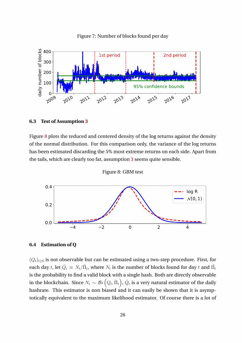
Figure 7: Number of blocks found per day

6.3 Test of Assumption 3

Figure 8 plots the reduced and centered density of the log returns against the density

of the normal distribution. For this comparison only, the variance of the log returns

has been estimated discarding the 5% most extreme returns on each side. Apart from

the tails, which are clearly too fat, assumption 3 seems quite sensible.

Figure 8: GBM test

6.4 Estimation of Q

(Qt)t≥0 is not observable but can be estimated using a two-step procedure. First, for

each day t, let Qt ≡ Nt/Πt, where Nt is the number of blocks found for day t and Πt

is the probability to find a valid block with a single hash. Both are directly observable

in the blockchain. Since Nt ∼ Bi(Qt, Πt

), Qt is a very natural estimator of the daily

hashrate. This estimator is non biased and it can easily be shown that it is asymp-

totically equivalent to the maximum likelihood estimator. Of course there is a lot of

26

variation across the daily estimates. We then smooth this new time series using a local

linear regression. Figure 9 shows we are not losing much information performing a

local linear regression over Q.

Figure 9: Estimation of Q

The two green curves are confidence bounds for the first step estimation if the true

(log (Q)t)t≥0 were the red curve (the second step estimate). If the erratic variations of

the first step estimation captured not only the first step estimation variance but also

some real variations of the hashrate not captured by the second step estimation, then

its variance should be bigger than the one resulting from the first step estimation error

only. Thus it should cross the green bounds much more often than 5% of the time,

which does not happen in our data. For the sake of clarity, we do not show the whole

series but the test works very well for the whole period.

27