we investigate how mother’s employment during childhood
TRANSCRIPT
econstorMake Your Publications Visible.
A Service of
zbwLeibniz-InformationszentrumWirtschaftLeibniz Information Centrefor Economics
Haaland, Venke Furre; Rege, Mari; Votruba, Mark
Working Paper
Nobody Home: The Effect of Maternal Labor ForceParticipation on Long-Term Child Outcomes
CESifo Working Paper, No. 4495
Provided in Cooperation with:Ifo Institute – Leibniz Institute for Economic Research at the University of Munich
Suggested Citation: Haaland, Venke Furre; Rege, Mari; Votruba, Mark (2013) : Nobody Home:The Effect of Maternal Labor Force Participation on Long-Term Child Outcomes, CESifoWorking Paper, No. 4495, Center for Economic Studies and ifo Institute (CESifo), Munich
This Version is available at:http://hdl.handle.net/10419/89644
Standard-Nutzungsbedingungen:
Die Dokumente auf EconStor dürfen zu eigenen wissenschaftlichenZwecken und zum Privatgebrauch gespeichert und kopiert werden.
Sie dürfen die Dokumente nicht für öffentliche oder kommerzielleZwecke vervielfältigen, öffentlich ausstellen, öffentlich zugänglichmachen, vertreiben oder anderweitig nutzen.
Sofern die Verfasser die Dokumente unter Open-Content-Lizenzen(insbesondere CC-Lizenzen) zur Verfügung gestellt haben sollten,gelten abweichend von diesen Nutzungsbedingungen die in der dortgenannten Lizenz gewährten Nutzungsrechte.
Terms of use:
Documents in EconStor may be saved and copied for yourpersonal and scholarly purposes.
You are not to copy documents for public or commercialpurposes, to exhibit the documents publicly, to make thempublicly available on the internet, or to distribute or otherwiseuse the documents in public.
If the documents have been made available under an OpenContent Licence (especially Creative Commons Licences), youmay exercise further usage rights as specified in the indicatedlicence.
www.econstor.eu

Nobody Home: The Effect of Maternal Labor Force Participation on Long-Term
Child Outcomes
Venke Furre Haaland Mari Rege
Mark Votruba
CESIFO WORKING PAPER NO. 4495 CATEGORY 4: LABOUR MARKETS
NOVEMBER 2013
An electronic version of the paper may be downloaded • from the SSRN website: www.SSRN.com • from the RePEc website: www.RePEc.org
• from the CESifo website: Twww.CESifo-group.org/wp T

CESifo Working Paper No. 4495
Nobody Home: The Effect of Maternal Labor Force Participation on Long-Term
Child Outcomes
Abstract We investigate how mother’s employment during childhood affects long term child outcomes. We utilize rich longitudinal data from Norway covering the entire Norwegian population between the years 1970 to 2007. The data allows us to match all family members and to measure maternal labor force participation throughout the child’s entire childhood. Our empirical approach exploits the variation in exposure to a working mother that exists across older and younger siblings in different family types. We compare sibling differences in families where the mother enters the labor force when the children are older and where the mother remains employed full time thereafter, to sibling differences in families where the mother remains out of the labor force during the entirety of her children’s adolescent years. Our identification strategy is, therefore, in the spirit of traditional difference-in-differences, the first difference pertaining to the differences in children’s ages within a family and the second pertaining to different family types. The analysis suggests that maternal labor force participation has significant and negative effects on years of education and labor market outcomes. However, the effects are small, which supports the notion that maternal labor force participation has, on average, a small effect on long-term outcomes for children.
JEL-Code: D130, J220.
Keywords: child development, household production, maternal labor force participation.
Venke Furre Haaland University of Stavanger / Norway
Mari Rege University of Stavanger / Norway
Mark Votruba Case Western Reserve University / USA
November 18, 2013 We are grateful for suggestions from a number of seminar participants. Financial support from the Norwegian Research Council (OF-10018) is gratefully acknowledged. Venke Furre Haaland would like to thank Statistics Norway for their hospitality during the work on this project.

1 Introduction
Dramatic increases in female labor force participation have changed the everydaylife of children dramatically during the last decades. In the United States in 1970,50 percent of women between 25-54 years were working. By 2008, this numberhad increased to 75 percent.1 In Norway, the focus of our study, more than 85percent of women between 25-54 years were working in 2009. In this paper weinvestigate how maternal employment during childhood ages of 1-16 affects long-term child outcomes.
Maternal employment can affect child development through at least four differ-ent channels. First, depending on the degree to which maternal care is substitutedfor by alternative care, it may affect the quality of care (Becker, 1991). The sub-stitutability will be contingent on the quality of both the maternal care and thealternative care.2 Second, to the extent that mother’s employment increases familyincome, the increased financial resources could have a positive effect on child de-velopment (e.g. Becker and Tomes, 1993; Duncan and Brooks-Gunn, 1997; Blau,1999; Baum and Charles, 2003; Dahl and Lochner, 2012). Third, if maternal em-ployment leads to increased stress level and tiredness, higher levels of parent-childconflicts and lower levels of parental acceptance might develop (Crouter and Bum-pus, 2001), which in turn could affect child development. Fourth, a mother’s partic-ipation in the labor force could affect the attitudes and aspirations of her children,especially for daughters (see e.g. Fernandez and Fogli, 2009; Fogli and Veldkamp,2011; Alesina et al., 2013).
To examine the relationship between maternal labor force participation andlong-term child outcomes, we utilize rich longitudinal data from Norway, coveringthe entire Norwegian population between the years 1970 to 2007. Importantly, thedata allow us to match all family members and to measure the maternal labor forceparticipation throughout the child’s entire childhood. Moreover, we measure long-term educational and labor markets outcomes, in addition to weight, height and IQfor boys at age 19.
Our empirical approach addresses problems of endogeneity by exploiting the
1OECD Labor Market Statistics: http://stats.oecd.org/2For example, Brooks et al. (2001) show that in cases where the alternative to maternal care is
unsupervised time at home, children of working mothers often have less discipline and less self-confidence. Yet, outcomes for some children may improve if working parents rely on high-qualityday-care programs and after-school care (e.g. Blau and Currie, 2006).
2
variation in exposure to a working mother that exists across older and younger sib-lings in different types of families. Many mothers choose to stay home or workpart time while they have young children at home but then permanently return tofull-time employment when the children are older. We refer to these families as En-ter Work (EW) families. In such families, older children systematically experiencefewer years of exposure to a working mother than do their younger siblings. Infamilies where the mother remains out of the labor force during the entirety of herchildren’s adolescent years, these systematic differences in exposure to a workingmother across older and younger siblings do not exist. We refer to these familiesas Never Work (NW) families. If longer exposure to a working mother affectschildren’s outcomes, we would expect, ceteris paribus, that the difference in out-comes observed for older and younger siblings would vary across the two familytypes. Our identification strategy is, therefore, in the spirit of traditional difference-in-differences, the first difference pertaining to the differences in children’s ageswithin a family and the second pertaining to the different family types. The crucialidentifying assumption is that relative age has identical effects on children’s out-comes in different types of families in the absence its effect on differential exposureto a working mom. Our rich data allow us to carefully investigate the plausibilityof this assumption by interacting relative age with several observable family andevent characteristics, as well as running placebo analyses.
Our analysis suggests that maternal labor force participation has a small butnegative and significant effect on years of education for the child. Our estimateindicates that each additional year of exposure to a mother who chooses to stay athome instead of work outside the home is predictive of an additional 0.013 yearsof education. Linearly extrapolating from this result suggests that 5 years of amother staying at home, as opposed to entering the labor force, is predictive of0.065 years of additional education for her child, which amounts to about 4 percentof the standard deviation in years of education. While such extrapolations haveto be interpreted with caution, this supports the notion that maternal labor forceparticipation has, on average, a very small effect on a child’s long-term education.We also find small effects of maternal labor force participation on a child’s long-term labor market outcomes.
There is a substantial body of literature investigating the effect of maternalemployment on child outcomes. Recent studies investigating the effect of mater-
3

nal employment during the child’s first year of life have utilized parental leavereforms to deal with the non-random selection into maternal employment (e.g.Carneiro et al., 2011; Baker and Milligan, 2010; Dustmann and Schönberg, 2012).Most studies of older children lack the same sophistication (Ruhm, 2008). Oneimportant exception can be found in studies evaluating welfare-to-work programs,which provide consistent evidence that maternal labor force participation is posi-tive for child development (Grogger et al., 2002). However, even if these studiesprovide compelling evidence for the population of welfare recipients, it is hardto generalize these results to the population at large. So far, the evidence for thebroader population is mixed (Datcher-Loury, 1988; Muller, 1995; Waldfogel et al.,2002; Anderson et al., 2003; James-Burdumy, 2005; Blau and Currie, 2006; Ruhm,2008). Similar to the approach in the present study, some of these studies investi-gate how maternal labor force participation affects children in family fixed effectsmodels (e.g. Waldfogel et al., 2002; James-Burdumy, 2005; Ruhm, 2008). An im-portant concern in these papers is that a mother’s decision to enter or exit the labormarket may depend on child characteristics (Ruhm, 2008). A second concern isthat the effect of birth order on child development varies across different familytypes (Kalil et al., 2012a). The rich registry data allow us to carefully address theseconcerns in our fixed effects framework. Finally, a general concern in fixed effectsmodels is that problems of attenuation bias—arising from measurement error in co-variates—become amplified. By focusing our analysis on the two types of families,EW and NW, our approach eliminates the problem of measurement error. This isbecause of the zero difference in mother’s labor force participation across siblingsfor the NW families, whereas for the EW families, the difference in mother’s laborforce participation is exactly equal to the children’s difference in age.
This paper is particularly related to Bettinger et al. (2013), who investigatea causal relationship between maternal labor force participation at ages seven toeleven and on the grade point average in tenth grade. In stark contrast to the presentstudy, Bettinger et al. (2013) demonstrate a very large, negative effect of maternallabor force participation on long-term child outcomes. In the concluding sectionwe discuss how the different findings may be due to the fact that the fixed effectsmodel in the present study estimates an average treatment effect, whereas the in-strumental variable approach in Bettinger et al. (2013) estimates a local averagetreatment effect (LATE) (Imbens and Angrist, 1994).
4

The remainder of this paper proceeds as follows: Section 2 presents the em-pirical approach, Section 3 describes the data, and Section 4 presents the results.Conclusions are offered in Section 5.
2 Empirical Strategy
To fix ideas, we start with the following stylized model:
Yi = α +βXi +θMWyrsi + ei, (1)
where Yi denotes the child’s long-term outcome (e.g. educational level, earn-ings, weight), Xi is a vector of fixed child and parental characteristics and MWyrsi isa measure of mother’s labor force participation during childhood. There are manyreasons why a child’s long-term outcomes may be correlated with the mother’s la-bor force participation during childhood. For instance, if mothers who work have(on average) greater human capital than mothers who do not, then the inheritabilityof ability would lead us to expect a positive correlation between mother’s work andchild outcome, independent of any causal relationship. As such, the coefficient γ inequation 1 is likely biased by unobserved characteristics of the mother that affectchild outcomes and are correlated with mother’s labor force participation.
We control for time-invariant maternal, paternal and family characteristics byexploiting the differential variation in exposure to a working mother that existsacross older and younger siblings in different family types. To implement ourstrategy, we define two types of families as follows:
1. Never Working (NW): Families with a mother who, for at least two of herchildren, does not work full time when her child is less than 19 years old.From these families, we drop any children who were less than 19 years oldwhen their mother enters full-time work.
2. Enters Work (EW): Families with a mother who does not work full timebetween the birth of her first child and the birth of her youngest child, butenters full-time employment by the time her youngest child turns 16 years,and then remains fully employed at least until her youngest child is 16 years
5

old. From these families we drop children who were older than 18 whentheir mother enters full-time work.
Group one (NW) is the comparison group. The age difference across siblings inthese families has no relationship with differences in exposure to a working mother.Group two (EW) is the treated group, in the sense that there is systematic variationin exposure to a working mom across older/younger siblings, determined by theirdifference in age.
If longer exposure to a working mother adversely affects child outcomes, thedifference in outcomes across older and younger siblings should favor the oldersibling more so in the EW families than in the NW families. As the existence ofbirth order effects is well-established, with earlier born siblings generally doingbetter than later-born ones (Black et al., 2011), we could also describe our hypoth-esis in terms of birth order gradients. Those gradients should be steeper amongEW families if longer exposure to a working mother is harmful to children.
We implement this empirical strategy by estimating the following model forthe outcome of child i in family s:
Yi,s = βs +βXi +ρRAi + γEWsRAi + ei, (2)
where βs captures family fixed effects, Xi captures observed individual-levelcharacteristics that vary across siblings (birth order interacted with family size,birth cohort interacted with gender, twin status, etc.), EWs is an indicator of familytype (defined above) and RAi captures the age of child i relative to the mean age ofhis/her siblings (relative age). Note that the direct effects of family type are sub-sumed by the inclusion of family fixed effects, while the inclusion of family fixedeffects leads to exact colinearity between relative age and mother’s age at birth.3
We are primarily interested in the coefficient γ , which captures the differentialeffect of relative age in EW families compared with NW families. If maternal la-bor force participation during childhood adversely affects child outcomes, then weshould see that γ>0, i.e. there should be a differential advantage of being an oldersibling in EW families compared with NW families.
3In our estimated models, we include quadratic controls for mother’s age at birth, and thereforeomit explicit controls for relative age.
6
The crucial identifying assumption is that the relationship between relative ageand child outcomes would be identical across EW and NW families if not for thedifferential exposure to a working mother that exists in EW families. This as-sumption is potentially undermined by the fact that family type is not assignedexogenously.
There are at least three situations that could challenge our identifying assump-tion. First, there could be a selection into EW based on the characteristics of theyoungest child relative to the characteristics of the older siblings.
For example, a mother may be more inclined to enter work if her youngerchildren are “performing well” relative to her older children. If so, the coefficientfor the interaction between EW and relative age would give a downward biasedestimate for the effect of differential exposure to a working mother.
Second, an event could affect selection into EW, which could bias the analysisif the event affects older and younger siblings differently. For example, a maritalconflict could be predictive of the mother’s decision to enter the labor market. Thiscould be problematic for our identifying assumption because marital conflict couldaffect siblings differently since they experience differential exposure to divorcedparents during their childhood. Third, there could be a selection into EW basedon parental characteristics. For example, it could be that more resourceful mothersare more likely to enter the labor force. This selection could bias our estimates ifbirth order effects (e.g. Black et al., 2011) differ across various family types. Ourrich data permit us to investigate the plausibility of our identifying assumption byincluding interactions between relative age with characteristics predictive of familytype, child ability and events. Moreover, we run placebo analyses to test whetherthe differential effect of relative age in EW families can be explained by differencesin mothers’ propensities for work.
3 Data
Our empirical analysis utilizes several registry databases provided by StatisticsNorway. We have a rich longitudinal data set containing records for every Norwe-gian from 1970 to 2007. The variables captured in this dataset include individualdemographic information (sex, age, marital status, number of children) and so-cioeconomic data (years of education, earnings). Importantly, the dataset includes
7

personal identifiers for one’s parents, allowing us to link children to their parentsand siblings.
We focus our analysis on the 1970-1980 birth cohorts in order to ensure avail-ability of outcome measures when the child reaches the age of 27. These cohortsamount to 590,312 native-born children who can be matched to both biologicalparents. In order to assure clean covariates for birth order and parity, we exclude62,326 children whose mother had children by more than one man. Another 73,690children are dropped to avoid capturing unusual living arrangements: We drop chil-dren who did not live in the same municipality as the father and the mother in thetime period when the child is between 5 and 16 years of age. To focus on differ-ential exposure to maternal employment we exclude an additional 1,495 childrenwhose mother or father died before the child reached 16 years of age.
We drop 157,046 children of families where the mother enters and/or exits full-time employment in a pattern that is inconsistent with the “family type” definitions(NW and EW) described in Section 2. To facilitate the utilization of family fixedeffects, we also drop 121,106 children who do not have any siblings represented inthe sample. Finally, avoiding issues arising from differential exposure to divorcedparents require us to drop from the sample 6,877 children of families where themother is not married to the father when the youngest child is 16. These restrictionsgive us a sample of 165,957 children in 77,581 families. About 38 percent of thesefamilies are EW types.
Our main outcome of interest is the child’s years of education at age 27. Assecondary outcomes, we also investigate high-school completion rates (≥12 yearsof education), college attendance rates (≥15 years of education) and log earningsat age 29. For boys, we also estimate effects for IQ score, height and body massindex (BMI) available (at age 19) from military records, which facilitates additionalplacebo tests.
Our key explanatory variable is an interaction term between relative age and anindicator for EW status (with NW status as the omitted group) as defined in Section2. Relative age refers to the child’s age relative to the mean age for all includedsiblings from a given family. For measuring EW status we utilize information onannual earnings4 to approximate full-time employment, as the data do not cover
4Annual earnings include wage, earnings from self-employment and work-related transfers, suchas sickness benefits, parental leave benefits, disability pensions and unemployment benefits.
8

work hours for the relevant time period. We follow previous studies (See Havnesand Mogstad, 2011a,b) by referring to an individual as employed full time in agiven year if he/she earns more than four “basic amounts” in that year. The “basicamount” is defined by the Norwegian Social Insurance Scheme.5 In 2007, one “ba-sic amount” corresponded to 72,000 NOK measured in 2009 prices (approximately12,200 USD). Mean and median earnings (of persons with earnings) in our sampleare 336,652 and 347,910 NOK, respectively, as measured in 2009 prices.
Our rich dataset allow us to construct several variables for capturing impor-tant child and family characteristics. Unless otherwise stated, we include the fol-lowing set of control variables in all models: family fixed effects, indicators forbirth cohort, child gender and gender/cohort interactions; indicators for birth or-der and birth order/family size interactions; an indicator for twin/triplet births; andquadratic covariates for mother’s age-at-child’s birth. Additional controls includedto evaluate the robustness of our estimates will be described during presentation ofour robustness results.
Table 1 presents summary statistics for key variables of interest. We separatelyreport the means and standard deviations for the NW and EW families. Comparingchildren in the EW families with the NW families, we can see that educationalattainments are higher for children from families where the mother enters work. Wealso see that in families where the mother enters work, parents’ education is higher,family earnings are higher, families are smaller and IQs are higher. The largedifferences in parental and family characteristics strongly indicate that a mother’sdecision to enter or exit the labor market is not a random event. Notably, however,with the inclusion of family fixed effects, this will only bias our estimates if birthorder effects (or, more precisely, if relative age effects) differ across various familytypes, which we will carefully investigate.
5The “basic amount” is used by the Norwegian Social Insurance Scheme to determine eligibilityfor and magnitude of benefits like old age pension, disability pension and unemployment compensa-tion. The “basic amount” is adjusted annually by the Norwegian Parliament to account for inflationand general wage growth.
9

4 Empirical Results
4.1 Descriptive Analysis
Table 2 presents estimates for the partial correlation between a child’s educationalattainment and mother’s employment during that child’s childhood, employingequation (1) as our estimation model, with MWyrs measured as years of full-timematernal employment over child ages 1-18. For comparison purposes, we ini-tially produce estimates over an unrestricted sample of Norwegian children bornin 1970-1980 before focusing on our main analytic sample.6 Conditional on theindividual-level covariates described above, column 1 demonstrates a strong cor-relation between maternal employment in childhood and child outcomes. Eachadditional year of maternal employment is predictive of a 0.056 increase in child’syears of education, suggesting a sizable, positive effect on child outcomes. How-ever, in column 2 we see that the size of partial correlation can largely be explainedby differences in other family characteristics which are correlated with MWyrs. Incolumn 2, when we add controls for parental characteristics and family size, thecoefficient on MWyrs decreases to 0.015. We generate similar results when werestrict the sample to children in NW and EW families (columns 3 and 4). Thus,the finding that mother’s employment is positively correlated with child outcomesholds true in our analytic sample to a similar degree as it does in the broader pop-ulation. Moreover, in our analytic sample, we again see that the apparent rela-tionship between mother’s employment and child outcomes is very sensitive to theinclusion of controls for family characteristics (see column 4).
The sensitivity of the MWyrs coefficient to inclusion of the family character-istics raises a strong concern about the role that family-level unobservables mightplay in biasing our results. Columns 5 and 6 demonstrate the legitimacy of suchconcerns. In column 5, we augment our family-level covariates with indicatorsfor the age of the mother’s youngest child when the mother returns to full-timework. The omitted category refers to NW families. The small, positive coefficientwe had estimated for MWyrs switches signs with the inclusion of these additionalcontrols. In column 6, when family fixed effects are controlled for, the estimated
6For the unrestricted sample in Table 2, we relax two of the sample restrictions defined in Section3. First, we relax the restriction to children of families where the mother enters and/or exits full-timeemployment in a pattern that is inconsistent with the EW and NW family types. Second, we do notrestrict the sample to children who have siblings represented in the sample.
10

coefficient on MWyrs becomes slightly more negative. Thus, as richer controls forparental characteristics are included, the correlation between mother’s employmentand child outcomes becomes increasingly negative. However, the estimated effectremains quite modest in size. From column 6, a one-year increase in exposure toa working mother is associated with a 0.025 increase in child education years, asmall effect relative to the standard deviation in education outcomes (2.1 years).
4.2 Main Results
Table 3 presents our main results, employing equation (2) as our estimation model.All models in this table include family fixed effects, as well as indicators forbirth order and birth order/family size interactions, an indicator for twin/tripletbirths, indicators for birth cohort and gender/birth cohort interactions and linearand quadratic terms for mother’s age at child birth. With the inclusion of fam-ily fixed effects, our covariate of interest, namely Relative age*EW, is (almost)perfectly collinear with the AWyrs covariate utilized in Table 2.7 Thus, it is unsur-prising that the coefficient on Relative age*EW in column 1 of Table 3 is nearlyidentical in magnitude to the coefficient on AWyrs in model 6 of Table 2, but ittakes the opposite sign. The coefficient on Relative age*EW can be interpreted asevidence for the causal effect of differential exposure to a working mother, underthe assumption that the “relative age gradient” in outcomes for children in EWand NW families would have been equal if not for the differential exposure. Theestimate in column 1 could be biased, however, if the size of the relative age gradi-ent differs systematically across various sorts of families. Columns 2-4 investigatethis by focusing on the systematic differences we documented across EW and NWfamilies (see Table 1).
In column 2, we include additional covariates by interacting parents’ educa-tion levels with child’s relative age. Consistent with results reported in Kalil et al.(2012a), we find that the relative age gradient in child outcomes tends to be steeperin families with higher parental education. As a result, our coefficient of interestdecreases somewhat in magnitude (to 0.013) in column 2. When we allow relativeage to exhibit heterogeneous effects along other predetermined individual or fam-
7Conditional on family fixed effects, AWyrs and Relative Age*AW are not perfectly collinearbecause AWyrs is measured in discreet units of years (Awyrs={0, 1, 2, . . . , 18}), while relative ageis a continuous variable. If not for this difference, Table 2/model 6 and Table 3/model 1 would haveproduced estimates identical in magnitude.
11
ily characteristics, this has virtually no effect on our estimate (see column 3). Incolumn 4, we include an additional covariate by interacting father’s mean earnings(measured over the years when the youngest child is 1-16 years old) with relativeage. This provides another robustness check for whether our estimate is biasedby the existence of steeper relative age gradients in families with higher socioeco-nomic status, but again it has no effect on our coefficient of interest.8 As a father’searnings are likely endogenous with his wife’s decision to work, we utilize themodel represented in column 3 of Table 3 as our preferred specification.
Our preferred specification implies that each additional year of maternal full-time employment during one’s childhood is associated with a 0.013 decrease inyears of education. Extrapolating from this result, we would predict that 5 addi-tional years of full-time employment by one’s mother reduces a child’s educationby 0.065 years, which amounts to 4 percent of a standard deviation in our sample.While such extrapolations have to be interpreted with caution, this supports thenotion that the mother’s labor force participation has a statistically significant, butquite small negative effect on children’s long-term educational attainment.
4.3 Robustness
The results in Table 3 allow us to be fairly confident that our estimate is not contam-inated by fixed differences across families, which lead to differential relative agegradients across EW and NW families. However, as discussed in Section 2, ouridentifying assumption could also be violated if the selection of mothers who enterthe labor force is affected by family events that affect younger and older siblingsdifferently. Two particular concerns in this regard are father’s job loss and maritalconflict, as both are known to be detrimental to children (see, e.g., Oreopouloset al., 2008; Amato, 2001; Rege et al., 2011) and could influence a mother’s de-cision to work. We address these issues in Table 4, with column 1 replicating theresult from our preferred specification for comparison.
Column 2 investigates potential bias arising from paternal job loss. In the ab-sence of an explicit measure for paternal job loss, we construct a proxy for job loss(DropIncomeF) based on whether the father experienced a large drop in income
8We have also interacted relative age with family income and fathers earnings at the time each ofhis children is between 1-16 years. None of these inclusions affect our coefficient of interest.
12

after the birth of his youngest child.9 We then include as an additional covariatethe interaction between this indicator and relative age. We can see that the coef-ficient on this additional covariate is insignificant and our coefficient of interest isunaffected.
In columns 3 and 4 we investigate potential bias arising from marital conflict.Again, we have no direct measure of marital conflict. So, to investigate the rolethat marital conflict could play, we modify our sample to include families withdivorced parents. Column 3 reveals that our estimate is only slightly larger in thisbroader sample (0.015). When we interact divorce with relative age, the coefficienton this interaction term is near zero and our coefficient of interest in unchanged(see column 4). This suggests that our preferred estimate is unlikely to be biasedby unobserved variation in marital conflict across families.
As a final test of potential bias, column 5 investigates the possibility that themagnitude of the relative age gradients in outcomes varies systematically with un-observed propensities for maternal employment. We do so by dividing the NWsample into three subgroups based on the number of years the mother spent in full-time employment over the years her youngest child is aged 20-35 (i.e. beyond theage where we would expect differential exposure to a working mother to influencechild outcome). In particular, NW1 identifies NW families where the mother had6-16 years of employment over this period, and NW2 identifies NW families wherethe mother had 1-6 years of employment.10 We then interact these indicators withrelative age and include them as controls in column 5. A finding that NW familiesexhibit steeper relative age gradients when the mother had greater post-childhoodemployment would present a serious challenge for the causal interpretation of ourmodel, since this would suggest that the gradient varies positively with mothers’propensity for work. However, we find no evidence of this. The relative age gra-dients in NW families appear unrelated to variation in (post-childhood) maternalemployment.
9The data do not cover job loss for the relevant time period. Hence we utilize information onannual earnings to approximate paternal job loss. Job loss is an indicator variable taking the value1 if the father experienced at least a 20 percent drop in earnings (compared to the mean of fatherearnings in the five years before the youngest child is born) in any of the years after the youngestchild is born and until the youngest child is 16 years of age.
10A third omitted category of NW families are those where the mother had no years of full-timeemployment over the years her youngest child was 20-35 years old.
13

4.4 Alternative Outcome Measures
In Table 5 we estimate the effect of maternal employment on other outcomes ofinterest: high-school completion rates, college attendance rates and log earnings.For each, we report estimates under our preferred specification (Table 3, column3). For both high-school completion and college attendance, we estimate effectsthat are statistically significant but small in magnitude, in line with our finding foryears of education. For instance, the result in column 1 implies that 5 additionalyears of full-time employment by one’s mother reduces the probability of the childcompleting high school by 1.5 percentage points, while reducing the probability ofthe child attending college by 2 percentage points (see column 2). The estimatedeffect of maternal employment on earning is somewhat larger, implying a 2.5 per-centage point decrease in earnings from 5 additional years of full-time employmentfor one’s mother.
4.5 Subsample Analysis, by Mother’s Education
In Table 6 we explore whether these estimated effects differ based on the educa-tional level of the mother. One motivation for this analysis is that mothers mightdiffer in their ability to provide a rich and stimulating environment for their chil-dren. For example, studies suggest that highly educated parents produce morecognitively stimulating home learning environments and more verbal and support-ive teaching styles (Harris et al., 1999). Moreover, highly educated parents spendmore time in activities believed to be more “developmentally effective” (Kalil et al.,2012b). If so, the detrimental effect of maternal employment on children’s out-comes might be expected to be larger for the children of more educated mothers.On the other hand, highly educated mothers, versus those with less education, maybe able to secure more effective and stimulating child care when they work, leavingus without a clear prediction.
Each cell in Table 6 presents the coefficient on the Relative age*EW covariateunder different regressions conducted separately for children of mothers with lowand high education. The outcome variable in these regressions is presented in theleft-hand column of the table. The estimated effect on years of education and onlog earnings is somewhat larger in magnitude for children of less educated mothers,although the differences are not statistically significant. The effect on high-school
14

completion rates appear somewhat larger for children of less educated mothers,while the opposite is true for college attendance. This likely reflects differencesin the underlying distribution of educational outcomes in the two subsamples. Re-gardless, only for the high-school completion outcome do we estimate a signifi-cantly different result for the two subsamples. For the children of less educatedmothers, this estimate suggests that 5 additional years of maternal employment ispredictive of a 3 percentage point decrease in the likelihood of completing highschool.
4.6 Subsample, Gender
As suggested, previous maternal employment may provide a positive role model ofa working mother, which may especially affect the aspirations of her daughter(s).Hence, we might expect the benefits of having a stay-at-home mother to be moremuted (or even possibly negative) for girls. Alternatively, several studies suggestthat girls benefit more from early child care than boys (see e.g. Melhuish et al.,2008). If the alternative care arrangement is formal child care, then the positiveeffect of having a stay-at-home mother could be smaller for girls than for boys.
Table 7 explores the existence of differential effects across boys and girls.Our first set of estimates (model 1) reflect models where gender-specific esti-mates are produced for the Relative age*EW covariates. This model also includesgender-specific controls for all the observed individual-level characteristics thatvary across siblings Xi (see Section 2) as well as parental education, but it main-tains the assumption that unobserved family characteristics have similar effects forboys and girls in a given family. The estimated effect on years of education andcollege attendance appears a bit larger for boys, although the difference is not sta-tistically significant. However, the effect of maternal employment appears to bemore detrimental to the subsequent earnings of girls than boys. The coefficient forgirls implies that 5 additional years of maternal employment is predictive of a 4percentage point decrease in the log earnings of girls.
The second set of results in Table 7 (model 2) estimates our preferred speci-fication,restricting our sample to boys and to families where at least two boys arepresent. With respect to the educational and earnings outcomes, the subsample ofboys produces generally smaller estimates than those derived in the pooled model.
As mentioned earlier, our estimates for the effect of maternal employment
15

could be biased if maternal employment decisions are affected by unobservablespredictive of differential outcomes for older versus younger siblings. For instance,if a mother is more likely to return to work when the prospects of success for heryounger children are (relatively) better, this would mute the estimate detrimentassociated with maternal employment. Limiting our sample to boys allows us totest outcomes related to this hypothesis, using measures of IQ and height avail-able from Norwegian military records. Both IQ and height are strong predictorsof subsequent economic outcomes (Cawley et al., 2001; Case and Paxson, 2008).If the selection process described above was operational, we should expect posi-tive coefficients on Relative age*EW for the IQ and height outcomes. Instead, weestimate small and insignificant coefficients (of opposite sign) for these outcomes.For completeness, we also estimate a model employing BMI as our outcome, andagain estimate a small, insignificant coefficient on our covariate of interest. Whilethese results are only specifically applicable to part of our analytic sample, they donot provide any evidence of bias arising from endogenous employment choices ofmothers.
4.7 Nonlinear Effects
In Table 8 we explore potential non-linearities in the effect of mother’s labor forceparticipation. Specifically, we explore whether differential exposure to a workingmother matters more at younger child ages, as the literature on early childhooddevelopment suggests (Carneiro and Heckman, 2003; Heckman, 2006). To in-vestigate this, we interact relative age with indicators for three subgroups of EWfamilies, defined based on age of the youngest child when the mother enters full-time employment. Estimates are reported for each of the four outcomes (as PanelsA-D), with estimates under our preferred specification reported in column 1 andgender-specific estimates reported in columns 2 and 3 (as in Table 7, model 1).
Notably, these estimates need to be interpreted with caution, as the timing ofthe mother’s work entry decision is likely not random and is potentially affected bythe development and maturity of the youngest child. If so, our effect estimates willbe biased downwards for families in which the mother enters the labor force earlyand upwards for families in which the mother enters the labor force late.
Perhaps because of this, we find that estimates are generally no larger for EWmothers who enter work at an earlier stage in the life of their youngest child. In fact,
16

for boys it appears that maternal employment is perhaps most detrimental to edu-cational outcomes during mid-adolescence rather than at earlier ages, although thesame does not appear true for earnings. Interestingly, for girls there is some indica-tion that the detrimental effect of maternal employment (on college attendance andearnings) is larger at earlier ages. Thus, while we refrain from drawing strong con-clusions from this analysis regarding the effect of maternal employment at differentages, our results do appear consistent with the existing childhood development lit-erature in one respect: Girls, as compared to boys, appear to be more influenced bydifferences in the early childhood environment (Melhuish et al., 2008).
5 Conclusion
Understanding how maternal work affects child development is important for coun-tries considering policies that either encourage or discourage maternal employ-ment. The Scandinavian countries, for example, provide paid parental leave withjob protection and high-quality, publicly subsidized day care as ways to encour-age females to maintain a close attachment to the labor force while their childrenare young. Many other OECD countries are now adopting similar policies, as in-creased female labor force participation is considered important for maintainingeconomic growth and sustainable pension systems in an aging population (Burni-aux et al., 2003).
This paper seeks to strengthen this understanding by analyzing how child de-velopment is affected by working mothers. The analysis exploits the variation inexposure to a working mother that exists across older and younger siblings in dif-ferent family types. We compare sibling differences in families where the motherenters the labor force when the children are older and where the mother remainsfully employed thereafter, to sibling differences in families where the mother re-mains out of the workforce during the entirety of her children’s adolescent years.The analysis suggests negative and significant effects of maternal labor force par-ticipation on years of education and labor market outcomes. However, the effectsare small, which supports the notion that maternal labor force participation has, onaverage, a small effect on children’s long-term outcomes.
Our small estimated effects of maternal labor force participation on long-termchild outcomes differ from those found by Bettinger et al. (2013), who investi-
17

gate a causal relationship between maternal labor force participation at ages 7 to11 and the grade point average (GPA) in tenth grade. For identification the studyutilizes a family reform in Norway which increased parents’ incentives to stayhome with their children, in an instrumental variable (IV) approach. The IV resultsdemonstrate that maternal labor force participation has a very large, negative effecton tenth grade GPA, which contrasts with the small, negative effect demonstratedin the present study. One plausible explanation for this is that the current paperestimates an average effect of an increase in maternal labor force participation,whereas Bettinger et al. (2013) estimate a local average treatment effect (LATE)(Imbens and Angrist, 1994). It may be that parents who expect to see the largestgains are the ones most likely to change their behavior in response to the familyreform. For example, if a child was struggling in school, the family reform mayhave presented an opportunity for a parent to stay at home and help the student.Norway’s educational system is characterized by short school days and extensivehomework assignments and an after-school care program with little scholastic fo-cus, so opportunities for helping a child with homework are significant.
Even if not conclusive, the present study indicates that mother’s labor forceparticipation has a small effect on the long-term outcome of the average child. Thesmall estimates are striking, as alternative care at the time of our study was informalchild care or unsupervised time at home, alongside the rather short supply of publicday care for the younger children. However, even if maternal employment has asmall effect on the average child, it is important to recognize that for some childrenparental care is not easily substituted (Bettinger et al., 2013). As such, in a worldwith historically high and still increasing female labor force participation, policiesthat provide high-quality care options for school children during parents’ workinghours could be positive for child development.
References
Alesina, A., Giuliano, P., and Nunn, N. (2013). On the origins of gender roles:Women and the plough. The Quarterly Journal of Economics, 128(2).
Amato, P. R. (2001). Children of divorce in the 1990s: An update of the amato andkeith (1991) meta-analysis. Journal of Family Psychology, 15(3):355–370.
18

Anderson, P. M., Butcher, K. F., and Levine, P. B. (2003). Maternal employmentand overweight children. Journal of Health Economics, 22(3):477–504.
Baker, M. and Milligan, K. (2010). Evidence from maternity leave expansionsof the impact of maternal care on early child development. Journal of HumanResources, 45(1):1–32.
Baum, I. and Charles, L. (2003). Does early maternal employment harm childdevelopment? an analysis of the potential benefits of leave taking. Journal ofLabor Economics, 21(2):409.
Becker, G. S. (1991). A treatise on the family. Harvard University Press, Cam-bridge, Mass. Enl. ed.
Becker, G. S. and Tomes, N. (1993). Human Capital and the Rise and Fall ofFamilies, chapter X., pages 257 – 298. University of Chicago Press, Chicago.3rd ed.
Bettinger, E., Hægeland, T., and Rege, M. (2013). Home with mom: The effectsof stay-at-home parents on children’s long-run educational outcomes. Journalof Labor Economics, Forthcoming.
Black, S. E., Devereux, P. J., and Salvanes, K. G. (2011). Older and wiser? birthorder and iq of young men. CESifo Economic Studies, 57(1):103–120.
Blau, D. and Currie, J. (2006). Pre-School, Day Care, and After-School Care:Who’s Minding the Kids?, volume Volume 2, chapter 20, pages 1163–1278. El-sevier.
Blau, D. M. (1999). The effect of income on child development. Review of Eco-nomics and Statistics, 81(2):261–276.
Brooks, J., Hair, E., and Zaslow, M. (2001). Welfare reforms impact on adoles-cents: Early warning signs. Washington DC: Child Trends.
Burniaux, J. M., Duval, R., and Jaumotte, F. (2003). Coping with ageing: a dy-namic approach to quantify the impact of alternative policy options on futurelabour supply in oecd countries. OECD Economics Department Working Papers371.
19
Carneiro, P., Løken, K., and Salvanes, K. (2011). A flying start or no effect?maternity leave benefi ts and long-term outcomes for mother and child. IZADiscussion Paper 5793.
Carneiro, P. M. and Heckman, J. J. (2003). Human capital policy. NBER WorkingPaper w9495, National Bureau of Economic Research.
Case, A. and Paxson, C. (2008). Stature and Status: Height, Ability, and LaborMarket Outcomes. Journal of Political Economy, 116:499–532.
Cawley, J., Heckman, J., and Vytlacil, E. (2001). Three observations on wages andmeasured cognitive ability. Labour Economics, 8(4):419 – 442.
Crouter, A. C. and Bumpus, M. F. (2001). Linking parents’ work stress to children’sand adolescents’ psychological adjustment. Current Directions in PsychologicalScience, 10(5):156–159.
Dahl, G. B. and Lochner, L. (2012). The impact of family income on child achieve-ment: Evidence from the earned income tax credit. The American EconomicReview, 102(5):1927–1956.
Datcher-Loury, L. (1988). Effects of mother’s home time on children’s schooling.The Review of Economics and Statistics, 70(3):367–373.
Duncan, G. J. and Brooks-Gunn, J. (1997). Consequences of growing up poor.Russell Sage Foundation, New York.
Dustmann, C. and Schönberg, U. (2012). The effect of expansions in maternityleave coverage on children’s long-term outcomes. American Economic Journal:Applied Economics, 4(3).
Fernandez, R. and Fogli, A. (2009). Culture: An empirical investigation of beliefs,work, and fertility. American Economic Journal: Macroeconomics, 1(1):146–77.
Fogli, A. and Veldkamp, L. (2011). Nature or nurture? learning and the geographyof female labor force participation. Econometrica, 79(4):1103–1138.
Grogger, J., Karoly, L., and Klerman, J. (2002). Consequences of Welfare Reform:A Research Synthesis. Santa Monica, CA:RAND.
20

Harris, Y. R., Terrel, D., and Allen, G. (1999). The influence of education contextand beliefs on the teaching behavior of african american mothers. Journal ofBlack Psychology, 25(4):490–503.
Havnes, T. and Mogstad, M. (2011a). Money for nothing? universal child care andmaternal employment. Journal of Public Economics, 95(11-12):1455–1465.
Havnes, T. and Mogstad, M. (2011b). No child left behind: Subsidized child careand children’s long-run outcomes. American Economic Journal: Economic Pol-icy, 3(2):97–129.
Heckman, J. J. (2006). Skill formation and the economics of investing in disadvan-taged children. Science, 312(5782):1900–1902.
Imbens, G. W. and Angrist, J. D. (1994). Identification and estimation of localaverage treatment effects. Econometrica, 62(2):467–475.
James-Burdumy, S. (2005). The effect of maternal labor force participation onchild development. Journal of Labor Economics, 23(1):177–211.
Kalil, A., Mogstad, M., Rege, M., and Vortuba, M. (2012a). Father presence andthe intergenerational transmission of educational attainment. Working paper.
Kalil, A., Ryan, R., and Corey, M. (2012b). Diverging destinies: Maternal ed-ucation and the developmental gradient in time with children. Demography,49(4):1361–1383.
Melhuish, E. C., Sylva, K., Sammons, P., Siraj-Blatchford, I., Taggart, B., Phan,M. B., and Malin, A. (2008). Preschool influences on mathematics achievement.Science, 321:157–188.
Muller, C. (1995). Maternal employment, parent involvement, and mathematicsachievement among adolescents. Journal of Marriage and the Family, 57(1):85–85.
Oreopoulos, P., Page, M., and Stevens, A. (2008). The intergenerational effects ofworker displacement. Journal of Labor Economics, 26(3):455–000.
Rege, M., Telle, K., and Votruba, M. (2011). Parental job loss and children’s schoolperformance. Review of Economic Studies, 78(4):1462–1489.
21

Ruhm, C. J. (2008). Maternal employment and adolescent development. LabourEconomics, 15(5):958–983.
Waldfogel, J., Han, W.-J., and Brooks-Gunn, J. (2002). The effects of early mater-nal employment on child cognitive development. Demography, 39(2):369–392.
22

Table 1: Summary statisticsNW EW p-value
Education years 13.40 (2.133) 13.96 (2.153) 0.000Completed high school 0.764 (0.425) 0.837 (0.370) 0.000College attendance 0.284 (0.451) 0.390 (0.488) 0.000Earnings 338.6 (166.8) 358.4 (173.0) 0.000Parental characteristicFather, education years 11.38 (2.080) 12.14 (2.403) 0.000Mother, education years 10.68 (1.382) 11.74 (1.948) 0.000Father, earnings (Child’s age 1-16) 426.8 (148.6) 456.3 (147.2) 0.000Mother, earnings (Child’s age 1-16) 145.5 (37.82) 272.5 (64.88) 0.000Father, age at birth 28.78 (5.530) 28.35 (4.825) 0.000Mother, age at birth 25.94 (4.742) 25.74 (4.196) 0.000Mother, age at birth (1 borne)Mother, birth cohort (year) 1948.5 (4.868) 1949.2 (4.374) 0.000Child characteristicsBirth cohort (year) 1974.4 (2.965) 1974.9 (2.919) 0.000Birth order 2.008 (1.046) 1.866 (0.864) 0.000Family size 3.049 (1.062) 2.669 (0.840) 0.000IQ 5.044 (1.733) 5.493 (1.735) 0.000Height in cm 179.6 (6.654) 180.1 (6.634) 0.000Body mass index 22.40 (3.176) 22.37 (2.998) 0.142Sample sizeN families 48,313 29,268N children 107,730 58,227Notes: Standard deviation in parentheses for mean statistics. Mother’s and father’s earn-ings reflect mean earnings from the period when the child is 1-16 years of age, measuredin NOK (2009)/1000. Family size reflects number of children in the family. Sample sizevaries for IQ and height due to missing observations; sample counts of boys with non-missing values for IQ and height are 53,005 for NW and 28,730 for EW.
23

Tabl
e2:
The
child
’sed
ucat
ion
and
mot
her’
sem
ploy
men
tsta
tus
(1)
(2)
(3)
(4)
(5)
(6)
MW
yrs
0.05
6**
0.01
5**
0.06
4**
0.02
0**
-0.0
18**
-0.0
25**
(0.0
007)
(0.0
008)
(0.0
015)
(0.0
015)
(0.0
049)
(0.0
051)
Add
ition
alco
vars
:In
divi
dual
char
acte
rist
ics
YY
YY
YY
Fam
ilych
arac
teri
stic
sY
YY
Indi
cato
rfor
EW
ayY
Fam
ilyfix
edef
fect
sY
Sam
ple
rest
rict
edto
:A
llA
llE
W/N
WE
W/N
WE
W/N
WE
W/N
WR
_squ
ared
20.
077
0.15
30.
075
0.15
20.
152
0.37
5O
bser
vatio
ns42
8,19
742
8,19
716
5,95
716
5,95
716
5,95
716
5,95
7N
otes
:OL
Sre
gres
sion
sw
ithro
bust
stan
dard
erro
rsin
pare
nthe
ses.
Dep
ende
ntva
riab
leis
year
sof
educ
atio
nat
child
age
27.I
ndiv
idua
lch
arac
teri
stic
s:In
dica
tor
cova
riat
esfo
rbi
rth
year
and
mal
e/bi
rth
coho
rtin
tera
ctio
ns,b
irth
orde
rin
dica
tor
cova
riat
esre
pres
entin
g(2
,3,
4,5,
6+)a
ndbi
rth
orde
rfam
ilysi
zein
tera
ctio
ns,i
ndic
ator
forc
hild
ren
born
intw
inor
trip
lebi
rths
and
linea
rcov
aria
tes
forr
elat
ive
age,
the
fath
er’s
and
mot
her’
sag
eat
birt
h.Fa
mily
char
acte
rist
ics:
Mot
her’
san
dfa
ther
’sed
ucat
ion;
year
sof
educ
atio
n(<
10,1
0–11
,12
–15,
≥16
)in
4x2
cate
gori
es,f
amily
size
indi
cato
rco
vari
ates
repr
esen
ting
(2,3
,4,5
,6+)
and
“Mot
hers
age
atbi
rth
offir
stbo
rn”
(lin
ear)
.Fo
rth
eun
rest
rict
edsa
mpl
e(a
ll),w
ere
lax
two
ofth
esa
mpl
ere
stri
ctio
nsde
fined
inSe
ctio
n3.
Firs
t,w
edr
opth
ere
stri
ctio
nto
child
ren
offa
mili
esw
here
the
mot
her
ente
rsan
d/or
exits
full-
time
empl
oym
enti
na
patte
rnth
atis
inco
nsis
tent
with
the
EW
and
NW
fam
ilyty
pes.
EW
/NW
cons
isto
four
mai
nan
alyt
icsa
mpl
ede
fined
inSe
ctio
n3.
Seco
nd,w
edo
notr
estr
ictt
hesa
mpl
eto
child
ren
who
have
sibl
ings
repr
esen
ted
inth
esa
mpl
e.M
Wyr
sis
ava
riab
lein
dica
ting
mot
her’
sw
ork
year
sov
erch
ildag
es1-
18.E
Way
are
16in
dica
tor
vari
able
sfo
rthe
age
ofth
eyo
unge
stch
ildw
hen
mot
here
nter
sfu
ll-tim
eem
ploy
men
t.T
heom
itted
cate
gory
refe
rsto
NW
fam
ilies
.
24

Table 3: Main results—effect on years of education
(1) (2) (3) (4)
Relative age*EW 0.024** 0.013* 0.013* 0.013*(0.0050) (0.0052) (0.0052) (0.0052)
Additional covars:Parents’ educ Y Y YBirth order*relative age Y YFamily size*relative age Y YM age at birth*relative age Y YM age at birthfirst*relative age Y YF earnings*relative age YR_squared2 0.375 0.376 0.376 0.376Observations 165,957 165,957 165,957 165,957
Notes: OLS regressions with robust standard errors in parentheses. Dependent variable isyears of education at child age 27. Relative age refers to the child’s age relative to the meanfor their included siblings. All models include family fixed effects, indicators for birthorder and birth order/family size interactions, an indicator for twin/triplets, indicators forbirth cohorts and male/birth cohort interactions linear and quadratic terms for mother’s ageat child birth. In columns 2-4 we include additional controls for relative age interacted withthe additional covars mentioned in the table. In particular, parents’ education representsmothers education and fathers education; years of education (<10, 10–11, 12–15, ≥16) in4x2 categories. Birth order and family size are indicator covariates representing (2, 3, 4,5, 6+). “mother’s age at birth” and “mother’s age at birth of first born” are linear terms.“Father’s earnings” is the log of father’s mean earnings from the period when the youngestchild is 1-16 years of age. MWyrs is a variable indicating mother’s work years over childages 1-16.
25
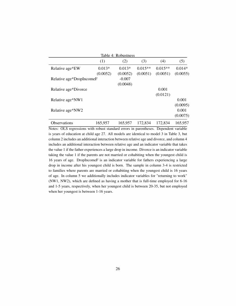
Table 4: Robustness(1) (2) (3) (4) (5)
Relative age*EW 0.013* 0.013* 0.015** 0.015** 0.014*(0.0052) (0.0052) (0.0051) (0.0051) (0.0055)
Relative age*DropIncomeF -0.007(0.0048)
Relative age*Divorce 0.001(0.0121)
Relative age*NW1 0.001(0.0095)
Relative age*NW2 0.001(0.0075)
Observations 165,957 165,957 172,834 172,834 165,957Notes: OLS regressions with robust standard errors in parentheses. Dependent variableis years of education at child age 27. All models are identical to model 3 in Table 3, butcolumn 2 includes an additional interaction between relative age and divorce, and column 4includes an additional interaction between relative age and an indicator variable that takesthe value 1 if the father experiences a large drop in income. Divorce is an indicator variabletaking the value 1 if the parents are not married or cohabiting when the youngest child is16 years of age. DropIncomeF is an indicator variable for fathers experiencing a largedrop in income after his youngest child is born. The sample in column 3-4 is restrictedto families where parents are married or cohabiting when the youngest child is 16 yearsof age. In column 5 we additionally includes indicator variables for "returning to work"(NW1, NW2), which are defined as having a mother that is full-time employed for 6-16and 1-5 years, respectively, when her youngest child is between 20-35, but not employedwhen her youngest is between 1-16 years.
26
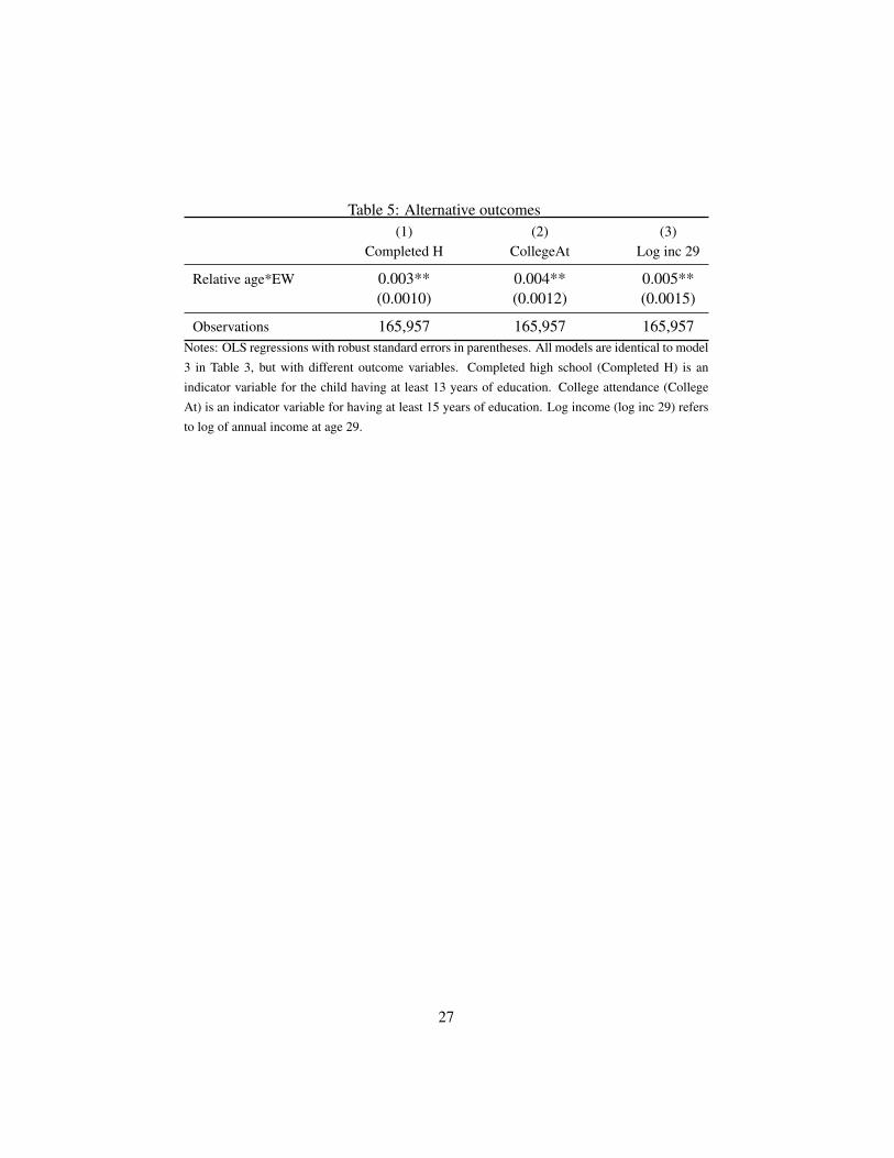
Table 5: Alternative outcomes(1) (2) (3)
Completed H CollegeAt Log inc 29
Relative age*EW 0.003** 0.004** 0.005**(0.0010) (0.0012) (0.0015)
Observations 165,957 165,957 165,957Notes: OLS regressions with robust standard errors in parentheses. All models are identical to model
3 in Table 3, but with different outcome variables. Completed high school (Completed H) is an
indicator variable for the child having at least 13 years of education. College attendance (College
At) is an indicator variable for having at least 15 years of education. Log income (log inc 29) refers
to log of annual income at age 29.
27

Table 6: Subsample, mothers education
(1) (3)Sample restriction, mothers education <11 years ≥11 years
Relative age*EWOutcome variables:Education years 0.018+ 0.011+
(0.0102) (0.0061)Completed H 0.006* 0.002+
(0.0024) (0.0011)College attendance 0.002 0.004**
(0.0021) (0.0015)Log income at age 29 0.007* 0.005*
(0.0029) (0.0018)
N 51,012 114,945Notes: OLS regressions with robust standard errors in parentheses. Each cell presents thecoefficient for the interaction between relative age and EW from different regressions. Allmodels are identical to model 3 in Table 3, but with different outcome variables.
28

Table 7: Subsample gender(1) (2)
Sample restricted to: Pooled sample Boys subsample
Relative age*EW: Girl coeffs Boy coeffsOutcome variables:Education years 0.010 0.016+ 0.004
(0.0090) (0.0084) (0.0096)Completed H 0.003+ 0.003+ 0.002
(0.0017) (0.0017) (0.0020)College attendance 0.002 0.005* 0.001
(0.0021) (0.0019) (0.0022)Log income at age 29 0.008** 0.002 0.001
(0.0025) (0.0025) (0.0029)
IQ 0.007(0.0082)
Height -0.007(0.0263)
BMI 0.004(0.0153)
N 165,957 49,551
Notes: OLS regressions, with robust standard errors in parentheses. Each cell presentsthe coefficient for the interaction between relative age and EW from different regressions.All models are identical to model 3 Table 3, but with different outcome variables, and inthe pooled model we include gender specific controls for all the observed individual-levelcharacteristics that vary across siblings (Xi) (see Section 2) as well as parental education.Sample size varies for IQ, height and BMI due to missing observations; sample counts ofboys with non-missing values for IQ is 47,469.
29

Table 8: Nonlinear effects on education and earnings
(1) (2) (3)Pooled sample
All Girl coeffs Boy coeffs
Panel A: Years of education
Relative age*EW age 0-9 0.009 0.012 0.005(0.0076) (0.0129) (0.0120)
Relative age*EW age 10-12 0.020** 0.011 0.030*(0.0075) (0.0127) (0.0120)
Relative age*EW age 13-16 0.010 0.009 0.011(0.0091) (0.0149) (0.0141)
Panel B: Completed high school
Relative age*EW age 0-9 0.003* 0.003 0.002(0.0014) (0.0024) (0.0023)
Relative age*EW age 10-12 0.004** 0.004+ 0.004+(0.0015) (0.0025) (0.0025)
Relative age*EW age 13-16 0.002 0.002 0.003(0.0018) (0.0029) (0.0028)
Panel C: College attendance
Relative age*EW age 0-9 0.003+ 0.005+ 0.001(0.0018) (0.0031) (0.0028)
Relative age*EW age 10-12 0.004* 0.001 0.008**(0.0018) (0.0030) (0.0028)
Relative age*EW age 13-16 0.002 0.000 0.004(0.0022) (0.0035) (0.0033)
Panel D: Log income at age 29
Relative age*EW age 0-9 0.006** 0.012** 0.002(0.0023) (0.0037) (0.0036)
Relative age*EW age 10-12 0.004+ 0.005 0.002(0.0023) (0.0036) (0.0037)
Relative age*EW age 13-16 0.006* 0.008* 0.003(0.0027) (0.0043) (0.0042)
Observations 165,957 165,957 165,957Notes: OLS regressions with robust standard errors in parentheses. All models are identicalto model 3 in Table 3, but with different outcome variables. EW category variables areconstructed based on the age of the youngest child when the mother enters work
30