wave–vortex interaction in rotating shallow water. …lmp/paps/kuo+polvani-jfm-1999.pdfwave{vortex...
TRANSCRIPT

J. Fluid Mech. (1999), vol. 394, pp. 1–27. Printed in the United Kingdom
c© 1999 Cambridge University Press
1
Wave–vortex interaction in rotating shallowwater. Part 1. One space dimension
By A L L E N C. K U O AND L O R E N Z O M. P O L V A N IDepartment of Applied Physics and Applied Mathematics, Columbia University,
New York, NY 10027, USA
(Received 1 December 1998 and in revised form 8 March 1999)
Using a physical space (i.e. non-modal) approach, we investigate interactions betweenfast inertio-gravity (IG) waves and slow balanced flows in a shallow rotating fluid.Specifically, we consider a train of IG waves impinging on a steady, exactly balancedvortex. For simplicity, the one-dimensional problem is studied first; the limitationsof one-dimensionality are offset by the ability to define balance in an exact way.An asymptotic analysis of the problem in the small-amplitude limit is performed todemonstrate the existence of interactions. It is shown that these interactions are notconfined to the modification of the wave field by the vortex but, more importantly,that the waves are able to alter in a non-trivial way the potential vorticity associatedwith that vortex. Interestingly, in this one-dimensional problem, once the waves havetraversed the vortex region and have propagated away, the vortex exactly recoversits initial shape and thus bears no signature of the interaction. Furthermore, weprove this last result in the case of arbitrary vortex and wave amplitudes. Numericalintegrations of the full one-dimensional shallow-water equations in strongly nonlinearregimes are also performed: they confirm that time-dependent interactions exist andincrease with wave amplitude, while at the final state the vortex bears no sign of theinteraction. In addition, they reveal that cyclonic vortices interact more strongly withthe wave field than anticyclonic ones.
1. IntroductionInteractions between fast inertio-gravity (IG) waves and slow balanced motions,
commonly referred to as ‘wave–vortex’ interaction, have been the subject of many re-cent studies. Whether such interactions exist, though, is still a partially open question.Dewar & Killworth (1995) have reviewed some of the seemingly contradictory resultsin the current literature and have pointed out that some of the discrepancies may bedue to fundamental differences between the various model equations that have beenstudied, while other discrepancies may simply be due to the use of different numericalschemes to solve the model equations.
While the question of whether and how IG waves interact with balanced motionsis not fully resolved, most theoretical approaches to date have made use of modaldecomposition and resonant wave interaction theory (Warn 1986; Yeh & Dong1988; Lelong & Riley 1991; Vanneste & Vial 1995; Bartello 1995; Majda & Embid1998). Related computational work (Errico 1984; Farge & Sadourny 1989; Yuan &Hamilton 1994; Dewar & Killworth 1995) has relied heavily on these same modaldecomposition tools. Such theoretical tools are rigorously applicable in the smallRossby or Froude number limit when the leading-order dynamics is linear. However,

2 A. C. Kuo and L. M. Polvani
the modal decomposition approach is difficult to extend to the nonlinear regime andmay also require assumptions on statistical homogeneity. Moreover, this approachprovides no direct, physical picture of how IG waves may interact with slow balancedmotions.
In this paper we attack the problem from a different angle. Rather than takingthe eigenmodes of some linearized set of equations as the fundamental constituentsof the interaction, we study actual physical objects. Specifically, we consider a trainof IG waves impinging on an isolated, exactly balanced vortex. Because the vortex isinitially steady, any changes to it can unequivocally be attributed to the IG waves:the extent to which the potential vorticity (PV) of the vortex is modified is the extentto which there exists a wave–vortex interaction. The results presented in this study areobtained in the context of the rotating f-plane shallow-water equations, the simplestmodel which permits both fast IG waves and slow balanced motions. By focusingon the physical evolution of the flow, we are able to directly pinpoint the time andlocation of the interaction and to observe and describe its physical characteristics.Moreover, our physical space approach is not limited to small Rossby or Froudenumber regimes and requires no assumptions of a statistical nature.
One study of wave–vortex interaction from a physical space viewpoint was carriedout by Ford (1994) who showed how IG waves can be generated from a balancedflow. In this paper, we focus on the reverse problem, namely how IG waves originallyexternal to a balanced flow are able modify it. Buhler & McIntyre (1998) have recentlyconsidered a similar problem in a channel on a β-plane and have shown that IGwaves forced at the boundary of the channel are able to irreversibly modify theinterior PV gradient.
In this work, we restrict our attention to wave–vortex interactions in one spatialdimension. With this simplification, the notion of ‘balance’ can be defined unambigu-ously, facilitating the analysis of the problem. The more complex two-dimensionalproblem will be discussed in a future work.
The paper is divided up as follows. In § 2 we set up the problem. An asymptoticanalysis is performed § 3, and the long-time interaction results are derived in § 4. Theasymptotic results are confirmed by numerical calculations in § 5, where we examinethe dependence of the interaction on the amplitudes of both the waves and the vortex,and the cyclonicity of the vortex. A brief discussion concludes the paper.
2. Problem setupThe rotating shallow-water equations (Pedlosky 1982), simplified by letting the
time-dependent variables be functions of a single spatial coordinate, x, are in non-dimensional form
∂u
∂t+ u
∂u
∂x+∂η
∂x− v = 0,
∂v
∂t+ u
∂v
∂x+ u = 0,
∂η
∂t+∂u
∂x+∂(ηu)
∂x= 0,
(1)
where u and v represent x and y velocity components respectively, and η represents thedeviation of the free surface from a (dimensional) mean height H . The non-dimension-

Wave–vortex interaction in rotating shallow water. Part 1 3
alization used here is standard (asterisks denote dimensional variables):
h∗ = H(1 + η), (u∗, v∗) = (√gH)(u, v), x∗ = Ldx, t∗ = (1/f)t,
where f is the Coriolis parameter, g the gravitational acceleration and Ld ≡ √gH/fis the Rossby deformation radius.
Although one-dimensional in space, the above shallow-water equations still containboth IG waves and balanced motions. These equations are thus the simplest startingpoint for studying wave–vortex interactions. Moreover, working with a single spatialdimension allows us to define balance in a unique way. Given the potential vorticityΠ of the flow, defined by
Π(x, t) ≡ vx(x, t) + 1
1 + η(x, t), (2)
one can invert for the balanced components of the flow ub, vb, and ηb, as follows.Geostrophic balance implies
ub = 0 and vb =∂ηb
∂x. (3)
Note that geostrophy is the only choice as a balance condition in one dimension; thisfollows from the fact that all spatially localized flows situated in an infinite domainthat are not geostrophic will adjust to eventually become steady and geostrophic. Intwo dimensions, on the other hand, this is not necessarily true. Using (3) to eliminatev from (2) yields an exact non-asymptotic potential vorticity inversion through thefollowing second-order boundary value problem for ηb:
∂2ηb
∂x2−Π(1 + ηb) + 1 = 0, (4)
together with appropriate evanescence boundary conditions. Thus the inversion con-sists in solving (4) for ηb, and then obtaining vb from (3). Of course, ub = 0.
To study wave–vortex interactions, we solve (1) with the initial conditions
u(x, t = 0) ≡ u(x, t = 0)
v(x, t = 0)η(x, t = 0)
= uW + uV , (5)
where
uW (x) =
uW (x− x0)00
(6)
and
uV (x) =
0vV (x)ηV (x)
. (7)
As sketched in figure 1, the initial flow is divided into two distinct regions. Nearx = 0 we place a localized potential vorticity anomaly, which we will refer to as
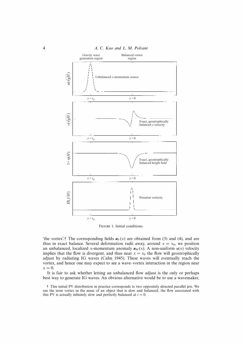
4 A. C. Kuo and L. M. Polvani
x = x0 x = 0
Potential vorticity
Π(f
/H)
x = x0 x = 0
Exact, geostrophicallybalanced height field1+
η(H
)
x = x0 x = 0
x = x0 x = 0
Unbalanced x-momentum source
Exact, geostrophicallybalanced y-velocity
Gravity wavegeneration region
Balanced vortexregion
u(√g
H)
v(√g
H)
Figure 1. Initial conditions.
‘the vortex’.† The corresponding fields uV (x) are obtained from (3) and (4), and arethus in exact balance. Several deformation radii away, around x = x0, we positionan unbalanced, localized x-momentum anomaly uW (x). A non-uniform u(x) velocityimplies that the flow is divergent, and thus near x = x0 the flow will geostrophicallyadjust by radiating IG waves (Cahn 1945). These waves will eventually reach thevortex, and hence one may expect to see a wave–vortex interaction in the region nearx = 0.
It is fair to ask whether letting an unbalanced flow adjust is the only or perhapsbest way to generate IG waves. An obvious alternative would be to use a wavemaker,
† This initial PV distribution in practice corresponds to two oppositely directed parallel jets. Weuse the term vortex in the sense of an object that is slow and balanced; the flow associated withthis PV is actually infinitely slow and perfectly balanced at t = 0.

Wave–vortex interaction in rotating shallow water. Part 1 5
i.e. to specify the fields at some boundary so as to satisfy some linearized waveequation. The problem, of course, is how one specifies boundary conditions when thelinearization assumption breaks down, an important regime we would like to explorein this paper. It is difficult to define general well-posed boundary conditions in thecase of large wave amplitudes. This follows from the fact that the characteristics for(1) are not simple straight lines unless wave amplitudes are small (Kuo & Polvani1997).
To overcome these difficulties, we have thus opted for generating IG waves asa byproduct of a geostrophic adjustment. In the small-amplitude limit, we recoverlinear rotating gravity waves (Gill 1982). At large amplitudes, these motions canstill be called IG waves, in the sense that they are fast and divergent; they nolonger, however, obey simple dispersion relations, and may have complicated shapesincluding discontinuities (i.e. shocks, see Houghton 1969). Irrespective of amplitude,therefore, we will refer to the motions emanating from a geostrophic adjustment asIG waves.
3. Asymptotic analysisWe begin our analysis of the problem by constructing asymptotic solutions to
(1) with initial conditions (5). This allows us to derive analytical expressions whichdescribe precisely when, where, and how wave–vortex interaction occurs in the small-amplitude limit. The large-amplitude extensions are treated numerically in § 5.
For purposes of deriving asymptotic solutions, we choose the following scalings forthe initial conditions:
uV (x) ≡ εuV (x), (8)
uW (x) ≡ ε2uW (x), (9)
where ε� 1. Other scalings are of course possible, but (8) and (9) are chosen becausethey provide the clearest possible scenario for wave–vortex interactions. Specifically,(8) eliminates the well-known vortex effect on waves via refraction (see Buhler &McIntyre 1998), while (9) pushes unwanted wave–wave effects (i.e. wave steepening)one order beyond the wave effects on the vortex, which are ultimately the main focusof this paper. The above scalings therefore clearly separate the exactly balanced vortexat lowest order, the IG waves arising solely from the unbalanced region at next order,and finally the nonlinear interaction of the two at third order.
3.1. Analysis of the field variables
Expanding the solution, as is customary, in the form
u(x, t) ≡ εu(1)(x, t) + ε2u(2)(x, t) + ε3u(3)(x, t) + O(ε4) (10)
and substituting into (1), yields the following sequence of problems.At O(ε)
∂u(1)
∂t+∂η(1)
∂x− v(1) = 0,
∂v(1)
∂t+ u(1) = 0,
∂η(1)
∂t+∂u(1)
∂x= 0, (11)
with initial conditions
u(1)(x, t = 0) = 0, v(1)(x, t = 0) = vV (x), η(1)(x, t = 0) = ηV (x). (12)

6 A. C. Kuo and L. M. Polvani
Since vV and ηV are already in geostrophic balance, it immediately follows that
u(1)(x, t) = 0, (13)
v(1)(x, t) = vV (x), (14)
η(1)(x, t) = ηV (x). (15)
Hence u(1) is simply the exactly balanced time-independent vortex.At O(ε2)
∂u(2)
∂t+∂η(2)
∂x− v(2) = 0,
∂v(2)
∂t+ u(2) = 0,
∂η(2)
∂t+∂u(2)
∂x= 0, (16)
with initial conditions
u(2)(x, t = 0) = uW (x− x0), v(2)(x, t = 0) = 0, η(2)(x, t = 0) = 0. (17)
The solution at this order is found, following Gill (1976), by eliminating v(2) and η(2)
in (16) to yield a single homogeneous dispersive wave equation for u(2)
∂2u(2)
∂t2− ∂2u(2)
∂x2+ u(2) = 0. (18)
Once u(2) is obtained via Fourier transforms, the solution for v(2) and η(2) can be foundin terms of it. The complete O(ε2) solution is
u(2)(x, t) =1
2√
2π
∫ ∞−∞UW (k)(e−i[kx+
√k2+1t] + e−i[kx−√k2+1t]) dk, (19)
v(2)(x, t) = −∫ t
0
u(2)(x, s) ds, (20)
η(2)(x, t) = −∫ t
0
∂u(2)(x, s)
∂xds, (21)
where UW (k) is the spatial Fourier transform of the initial condition
UW (k) =1√2π
∫ ∞−∞uW (x− x0)e
ikx dx. (22)
At this order the solution is identical to that obtained from a linear, time-dependentgeostrophic adjustment problem (Cahn 1945). Therefore, we refer to u(2)(x, t) as pureIG waves because they originate solely from the unbalanced region near x = x0 andare independent of the vortex part of the solution u(1). If the analysis were to stop atthis order, one would conclude that no wave–vortex interaction exists.
However, at O(ε3)
∂u(3)
∂t+∂η(3)
∂x− v(3) = 0,
∂v(3)
∂t+ u(3) = −u(2) ∂v
(1)
∂x,
∂η(3)
∂t+∂u(3)
∂x= −∂(η(1)u(2))
∂x. (23)
with initial conditions
u(3)(x, t = 0) = 0, v(3)(x, t = 0) = 0, η(3)(x, t = 0) = 0. (24)
Again, eliminating v(3) and η(3) from (23) yields a single inhomogeneous dispersive

Wave–vortex interaction in rotating shallow water. Part 1 7
wave equation for u(3),
∂2u(3)
∂t2− ∂2u(3)
∂x2+ u(3) = IWV (x, t), (25)
where the inhomogeneous term IWV (x, t) is given by
IWV = −u(2) ∂v(1)
∂x+∂2(η(1)u(2))
∂x2. (26)
This source term (26) contains products of u(1) (the vortex) and u(2) (the IG waves), andtherefore can only be interpreted as a wave–vortex interaction term. The interaction,as (25) shows, is essential to generating the third-order solution, since IWV becomesnon-zero only when the IG waves enter the vortex region near x = 0. We solve (25)using Duhamel’s principle (John 1978), and thus obtain the complete O(ε3) solution
u(3)(x, t) =1
2√
2π
∫ t
0
[∫ ∞−∞
iIWV (k, s)√k2 + 1
(e−i[kx+√k2+1(t−s)] − e−i[kx−√k2+1(t−s)]) dk
]ds,
(27)
v(3)(x, t) = −∫ t
0
(u(3)(x, s) + u(2)(x, s)
∂vV
∂x
)ds, (28)
η(3)(x, t) = −∫ t
0
(∂u(3)(x, s)
∂x+∂(ηvu
(2)(x, s))
∂x
)ds, (29)
where IWV is the spatial Fourier transform of IWV .To sum up the asymptotic analysis: since the lowest-order solution u(1) consists of
a balanced vortex only, and the next-order solution u(2) consists of IG waves only, weconclude that the generation of u(3) by the previous two establishes the existence of a‘wave–vortex’ interaction.
The question, at this point, is whether the IG waves modify the vortex, vice versa, orboth. In other words, how do we interpret u(3)? Considering the fact that the Poincarewave operator appears on the left-hand side of (25), one might argue that u(3) issimply IG waves. However, the same operator appears at all orders of perturbationbeyond lowest order. Almost by definition then, since the vortex solution at lowestorder is time independent, one would be forced to conclude that the vortex modifiesthe IG waves but not vice versa.
However, from (23), it is unclear whether the u(3) solution contains only IG waves:a balanced component could be present, in which case we would have to concludethat IG waves affect the vortex as well. It turns out that this conclusion is the correctone, and is revealed through an analysis of the potential vorticity.
3.2. Analysis of the potential vorticity
Substituting the formal ansatz (10) into the definition (2) implies the followingexpression for the potential vorticity Π(x, t):
Π(x, t) = Π (0) + εΠ (1) + ε2Π (2) + ε3Π (3) + O(ε4), (30)
where
Π (0) = 1, (31)

8 A. C. Kuo and L. M. Polvani
Π (1) = v(1)x (x)− η(1)(x), (32)
Π (2) = −η(1)(x)Π (1) + v(2)x (x, t)− η(2)(x, t), (33)
Π (3) = ((η(1)(x))2 − η(2)(x, t))Π (1) + v(3)x (x, t)− η(3)(x, t). (34)
Π (0), the lowest order PV, is simply the background value f/H properly non-dimen-sionalized. Π (1) is the linearized PV associated with the u(1) solution (the initial vortex),and is time independent. Π (2) appears to be time dependent, but it is not. Since (16)implies
∂(v(2)x − η(2))
∂t= 0, (35)
and since (v(2)x − η(2)) vanishes at t = 0, the expression for Π (2) reduces to
Π (2) = −η(1)(x)Π (1), (36)
which explicitly shows the time independence. The u(2) fields are just linear IG wavesand hence, as is commonly believed, ‘carry’ no PV. To O(ε2) therefore, the PV is timeindependent and is solely associated with the initial vortex.
The interesting result is seen at O(ε3). We can show explicitly that Π (3) is timedependent, and therefore the u(3) fields do in fact ‘carry’ PV. From (23), one mayderive an expression for (v(3)
x − η(3)) in terms of the O(ε2) variables. Substituting thatexpression into (34) yields a simpler expression for Π (3):
Π (3) = η(1)(x)2Π (1) + v(2)(x, t)Π (1)x (37)
which is explicitly time dependent, and thus demonstrates that the IG waves canaffect the vortex.
Alternatively, one may deduce this fact by examining the equation for the evolutionof PV:
∂
∂tΠ(x, t) + u
∂
∂xΠ(x, t) = 0, (38)
which up to O(ε2) yields
∂
∂tΠ (0) =
∂
∂tΠ (1) =
∂
∂tΠ (2) = 0 (39)
but at O(ε3) yields
∂
∂tΠ (3) = −u(2) ∂
∂xΠ (1). (40)
This evolution equation shows how the nonlinear coupling of the PV associated withthe vortex, Π (1), and the velocity field due to the incoming IG waves, u(2), produceschanges in the PV, which given our scaling choices (8)–(9), occurs only at O(ε3) here.
3.3. Analysis of the energy
The key effect of waves on the vortex is described by equation (40). In this subsection,for completeness, we provide a further description of the interaction in terms of theenergy exhange between the waves and the vortex. The total energy is defined by
E = 12(u2 + v2)(1 + η) + 1
2(1 + η)2, (41)

Wave–vortex interaction in rotating shallow water. Part 1 9
and it obeys the conservation law (Whitham 1974)
∂E
∂t+
∂
∂x
[12(u3 + uv2)(1 + η) + u(1 + η)2
]= 0. (42)
Substituting (10) into (42) and collecting terms at different orders in ε yields equationsat even powers of epsilon (the odd powers yield trivial identities through O(ε5)).
At O(ε2) one obtains
∂E(1)
∂t= 0, (43)
where E(1) ≡ 12(u(1)2 + v(1)2) + 1
2η(1)2. At lowest order, the energy† is only associated
with the vortex and, since the vortex is balanced, the energy is time independent.At O(ε4), the energy equation takes the form
∂E(2)
∂t+∂(u(2)η(2))
∂x= 0, (44)
where E(2) ≡ 12(u(2)2 + v(2)2) + 1
2η(2)2. This equation, identical to the one found in Gill
(1982), reflects the simple fact that, at this order, the time change in energy in a regionis solely due to the IG wave flux in and out of that region. Thus, at this order, thereis no interaction between the IG waves and the vortex.
Finally, at O(ε6), one obtains the energy equation associated with the third-ordersolution:
∂E(3)
∂t+∂(u(3)η(3))
∂x= −v(3)u(2) ∂v
(1)
∂x− η(3) ∂(η(1)u(2))
∂x, (45)
where E(3) = 12(u(3)2 + v(3)2) + 1
2η(3)2. This energy equation differs from the previous
two. At this order, E(3) changes either because of a flux or due to an interaction ofthe first- and second-order solutions (cf. the right-hand side of (45), remembering thatthe O(ε3) solution is created solely from the interaction of the first- and second-ordersolutions). In other words, E(3) is created or destroyed when the IG waves come incontact with the initially balanced vortex. Hence, at this order, there is an energyexchange between waves and vortices.
3.4. An illustrative example of wave–vortex interaction
We now graphically illustrate this wave–vortex interaction by plotting, for a specificinitial condition, the asymptotic solutions given in § 3.1 and § 3.2. As already men-tioned, the initial condition is composed of an exactly balanced vortex part, uV = εuV ,and an unbalanced part, uW = ε2uW , which generates IG waves (see figure 1 for aschematic view).
The vortex part is specified initially as the solution of
d2ηV
dx2− ηV =
1
2
(tanh
[(x+ 1
2)
SV
]+ tanh
[(−x+ 1
2)
SV
]), (46)
vV =dηVdx
, (47)
uV = 0. (48)
† Note that the quantities E(i), as defined above at each order, are not the coefficients of thepowers of ε that appear upon substituting (10) into (41).

10 A. C. Kuo and L. M. Polvani
These initial conditions on uV correspond to a positive tanh ‘bump’ in the potentialvorticity field, roughly one deformation radius wide. The two equations (46) and (47)represent the exact balance procedure given in § 2 at O(ε). The steepness of the edgesof this bump is controlled by the parameter SV . For illustrative purposes, we chooseSV = 0.2.
For the unbalanced component, we specify
uW (x) = e−(x−x0)2
, vW (x) = 0, ηW (x) = 0. (49)
This unbalanced component of the initial conditions will cause IG waves to begenerated from the region near x = x0. We choose x0 large enough so that theunbalanced region is well separated from the vortex at t = 0. For the results presentedin this paper we have set x0 = −14.
The asymptotic solution is plotted in figure 2. The left column shows the heightfield at five different times and the right column shows the corresponding PV. In eachframe, the first three orders of perturbation are plotted. For clarity, the curves for theheight field have been offset from their zero mean.
Consider first the height fields. At t = 10 the exactly balanced initial vortex (dasheddotted line) and the linear IG wave train (dashed line) impinging on it from the left,though close, have not yet interacted. The third-order solution (solid line) is thereforeidentically zero. By t = 15 the IG waves have reached the vortex and their interactionhas generated the third-order solution. At t = 25, the IG waves are seen leaving thevortex region, and the third-order solution resulting from the wave–vortex interactionis composed of transmitted waves (relatively strong) and reflected waves (relativelyweak). Hence it is clear that the presence of the vortex modifies the total IG wavefield. Such effects of the balanced motion on IG waves is well known (see for instanceDewar & Killworth 1995 or Buhler & McIntyre 1998) but in this case, the effect ispurely nonlinear rather than due to refraction or linear reflection.
Note most importantly that the IG waves affect the vortex as well. To see this,consider the evolution of the potential vorticity in figure 2. As already mentioned,the PV is time independent at first and second order; we plot these for reference.The effect of waves on the PV appears at O(ε3). Notice that Π (3) becomes timedependent only around t = 15, after the IG waves have entered the vortex region,thus demonstrating explicitly that IG waves alter the vortex.
It is important to remark that the appearance of wave–vortex interactions atO(ε3) in this analysis is not a fundamental property of the interaction. It is simply anartifact of our scaling choices (8) and (9), which are guided by our interest in isolatingwave–vortex interactions from wave–wave interactions. The latter are easily treated bystandard perturbation techniques (Kevorkian & Cole 1981). Our scaling choices simplyrelegate wave–wave interaction to O(ε4). It is easy to show that the alternative scalingchoice uV ∼ uW ∼ ε leads to a conventional advective Rossby number expansion ofthe shallow-water equations, in which case ε can be interpreted as a Rossby number.With that more conventional scaling, wave–vortex interactions would appear at O(ε2)(together with wave–wave interactions). It would then follow that, at small Rossbynumber, wave–vortex interactions scale like the square of the Rossby number.
4. The limit t→∞Having described how IG waves interact with a balanced vortex as they impinge
upon it, we now turn our attention to the question of whether this interaction leavesa long-time signature on the vortex after the IG waves have propagated away from

Wave–vortex interaction in rotating shallow water. Part 1 11
0
–0.25
–0.50
–0.75
–1.00
–10 –5 0 5 10
x(√gH/f )
0
–0.25
–0.50
–0.75
–1.00
0
–0.25
–0.50
–0.75
–1.00
0
–0.25
–0.50
–0.75
–1.00
0
–0.25
–0.50
–0.75
–1.00
η(1)
η(2)
η(3)
η = εη(1) + ε2η(2) + ε3η(3) + O(ε4)
0.8
0.6
0.4
0.2
0
–2 –1 0 1 2
x(√gH/f )
Π (1)
Π (2)
Π (3)
Π = 1+ εΠ (1) + ε2Π (2) + ε3Π (3) + O(ε4)
t = 40
0.8
0.6
0.4
0.2
0
t = 25
0.8
0.6
0.4
0.2
0
t =15
0.8
0.6
0.4
0.2
0
t = 10
0.8
0.6
0.4
0.2
0
t = 0
Figure 2. Time evolution of the height and potential vorticity asymptotic solutions during awave–vortex interaction. For the perturbation height plots, the η(2) and η(3) solutions have beenoffset from their zero mean values by −0.5 and −1.0 respectively. The vortex parameter SV = 0.2.Π (1) and Π (2) are time independent, and plotted for reference only.

12 A. C. Kuo and L. M. Polvani
the vortex. We first show, in the asymptotic limit treated in the previous section, thatthe IG waves leave no trace on the vortex. This is accomplished by showing that inthe limit t→∞, the time-dependent O(ε2) and O(ε3) solutions vanish so that the fullsolution (up to this order) reduces to the steady O(ε) vortex solution. Second, weshow that this long-time non-interaction result must hold to all orders in ε. In eithercase, we need make no assumption on the form of the vortex (other than it being inexact balance), or the initially unbalanced wave-generation region. We conclude thissection with a brief discussion clarifying why this surprising no-net-interaction resultis not necessarily a consequence of the one-dimensional nature of our problem.
4.1. The small-amplitude case
To show that in the limit t → ∞ the O(ε2) solutions vanish, it is more convenientto work directly with the equations of motion, rather than taking the limit of theexplicit solutions (19)–(21). The only steady bounded solution to (18) is u(2) = 0. Tofind η(2)(x, t) and v(2)(x, t) in the limit t → ∞, one may drop the time-derivative andu(2) terms in (16), yielding geostrophic balance at the final state:
η(2)x (x,∞) = v(2)(x,∞). (50)
This is the familiar geostrophic degeneracy problem (Gill 1982). To close the system,one needs an extra equation. Using (35) and (17) it follows that
v(2)x (x,∞)− η(2)(x,∞) = v(2)
x (x, 0)− η(2)(x, 0) = 0. (51)
Now (50) and (51) are used to solve for v(2) and η(2) at steady state. Eliminating v(2)
yields
η(2)xx (x,∞)− η(2)(x,∞) = 0. (52)
The requirement that the solution be bounded at |x| → ∞ again implies thatη(2)(x,∞) = 0 and thus v(2)(x,∞) = 0. Hence in the limit t → ∞ the entire O(ε2)solution vanishes.
Next, we show that the O(ε3) fields also vanish in the limit t→∞. That u(3) vanishesin that limit is immediately seen from (25) and the fact that IWV (x,∞) = 0. As forη(3) and v(3), one has again
η(3)x (x,∞) = v(3)(x,∞). (53)
Moreover, (23) implies that
∂(v(3)x − η(3))
∂t= −u(2) ∂
2v(1)
∂x2− ∂u(2)
∂x
∂v(1)
∂x+∂(η(1)u(2))
∂x, (54)
which we integrate with respect to t to obtain
v(3)x (x, t)− η(3)(x, t) = P (x, t), (55)
where
P (x, t) ≡ −[(v(1))x − η(1)]x
∫ t
0
u(2)(x, s) ds− [(v(1))x − η(1)]
∫ t
0
u(2)x (x, s) ds
= [(v(1))x − η(1)]x v(2)(x, t)− [(v(1))x − η(1)] η(2)(x, t).
In the limit t→∞, v(2) and η(2), and therefore P (x, t), vanish. It follows from (53) and(55) that v(3) = η(3) = 0.
The conclusion here is that in the limit t→∞, the full solution to O(ε4) is identicalto u(1). In other words, the initially balanced vortex reappears intact at long times
Wave–vortex interaction in rotating shallow water. Part 1 13
after the waves have propagated away. This non-trivial result is illustrated in figure 3,where we plot the long-time continuation of the asymptotic solution shown in figure2. At t = 1400 (last row of figure 3) the total height and PV fields are indistinguishablefrom their initial values.
For large (but not infinite) t, however, the time-dependent component of the PV,i.e. Π (3), is associated with a kink in the η(3) solution around x = 0 (see for instanceframe t = 200 in figure 3). This kink is the long-time signature of the wave–vortexinteraction. The rate at which this kink disappears is the rate at which the term P (x, t)in (55) goes to zero. Since the O(ε2) fields vanish as t−1/2 in the limit t → ∞ (Gill1982), the signature of wave–vortex interaction disappears at that rate. Note that nosuch kink appears in η(2) at large t since (51), in contrast to (55), has a homogeneousright-hand side.
4.2. The case of arbitrary amplitude
This surprising ‘no net interaction’ result can be extended to the case of arbitraryamplitudes. The proof follows Rossby (1938), who studied the adjustment of a locallyunbalanced momentum source. We do likewise except that our initial conditionincludes, in addition to the unbalanced momentum source, a region of exact balance(the vortex). Following Rossby, we adopt a Lagrangian description of the fluid.Geostrophic balance, together with conservation of y-momentum and mass betweenthe initial (subscript ‘0’) and final (subscript ‘∞’) states imply
dη∞dx∞
= v∞, (56)
v∞ − v0 = x0 − x∞, (57)
(1 + η∞)dx∞dx0
= 1 + η0, (58)
where x0 and x∞ are, respectively, the initial and final positions of each Lagrangianfluid column. One may eliminate η∞ and v∞ from the above to obtain a singleequation† for x∞:
(1 + η0)
(d
dx∞
)2
x0 +dη0
dx∞dx0
dx∞− x0 + x∞ − v0 = 0. (59)
This equation could in principle be solved to obtain x∞(x0). The crux, however, isthat this equation does not contain u0. This implies that any initial x-momentum hasno effect on the final solution. In particular, if η and v are initially in geostrophicbalance, as they are in our problem, then the solution to (59) is simply x∞ = x0, inwhich case (57) and (58) imply that initial and final values of η and v are identical.Thus, although any unbalanced initial x-momentum source can be used to generatearbitrary IG waves (which eventually must impinge on the vortex), the IG wavesleave no signature on the final state.
That u0 does not appear in (59) is a result of the restriction of no y variations: u0
displays no direct PV signature. Thus, the objection might be raised as to whether thenon-interaction result holds if we take the initial region of imbalance to be associatedwith a non-trivial potential vorticity. We argue that the answer is still affirmative, butfirst we make clear a certain facet of the problem.
† Rossby derived this equation for the case η0 = 0 (no initial height perturbations) in which casethe equation becomes linear. See also Boss & Thompson (1995) for the axisymmetric top-hat case.

14 A. C. Kuo and L. M. Polvani
0.1
0
–0.1
–0.2
–0.3
–10 –5 0 5 10
0.08
0.04
0
–0.04
–0.08
0.08
0.04
0
–0.04
–0.08
0.08
0.04
0
–0.04
–0.08
0.08
0.04
0
–0.04
–0.08
η(2)
1.12
1.08
1.04
1.00
–2 –1 0 1 2
Π (3)
t =1400
0.15
0.10
0.05
0
–0.05
t =1400
0.15
0.10
0.05
0
–0.05
t = 600
0.15
0.10
0.05
0
–0.05
t = 200
0.15
0.10
0.05
0
–0.05
t =100
–0.4
η
η(x, t = 0)
η(3) Π (3)(x, t = 0)
Π
Π(x, t = 0)
x(√gH/f )x(√gH/f )
Figure 3. Continuation of figure 2 for long times. For the height plots, η(0) is no longer plotted andthere is no offset as in previous plot. For the potential vorticity plots, we plot only Π (3)(x, t) andits initial value, omitting the steady Π (0), Π (1) and Π (2) fields. The two plots in the last row showthe full perturbation solution to O(ε4) at t = 1400 along with the initial conditions, where we havechosen ε = 0.1.

Wave–vortex interaction in rotating shallow water. Part 1 15
Assume initial spatial η or v-velocity variations in the unbalanced region (asopposed to a u variation) which are not exactly balanced. As such, these fields willgive rise to IG waves and be associated with non-trivial PV. The PV associatedwith this local region of imbalance must be physically distinguishable from thePV associated with the localized vortex so that unequivocally one may state thisis a problem of an external IG wave interacting with a separate and distinct PVdistribution. If such is the case, one may again state that only an exponentially smallnet long-term wave–vortex interaction will take place. This is because the influenceof PV anomalies on the displacement of material particles in the fluid is confined toa few deformation radii (Rossby 1938; Blumen 1972). Specifically, Rossby’s originalLagrangian method showed that net material fluid displacements associated withlocalized unbalanced PV anomalies decrease exponentially with distance from thoseanomalies. The exponential fall off rate is given by the deformation radius. Thus, thefurther one is from the IG wave source, the smaller the net interaction.
Note that moving the IG wave source further away from the vortex is not equivalentto requiring the IG waves to be smaller in amplitude. One could take Rossby’s (1938)v-jet initial conditions for the unbalanced source, simultaneously increase the distancefrom the balanced region and increase the amplitude of the v-jet to obtain IG wavesof roughly constant amplitude at a fixed distance from the wave source region.
Finally, note that implicit in the arguments presented in this section is that flowsin a one-dimensional infinite domain actually become steady. We have no formalproof of this. However, numerical integrations of the full shallow-water equations (asshown in § 5) support this assumption: we have never observed perpetual generationof gravity waves at the expense of the energy of the vortex. In addition, the asymptoticresults presented in § 3.1 are consistent with the claim that the oscillatory gravity wavesolutions decay in time, and the flow eventually becomes steady.
4.3. Discussion
We do not believe that this long-time result is obvious. Consider: why should ar-bitrarily large IG waves not be able to alter the potential vorticity of the flow, e.g.through Stokes drift? We have shown in the small-amplitude limit, and will shownumerically for the case of large amplitudes, that the PV does change in time whenthe IG waves hit the vortex. However, the net long-time change always turns out tobe zero.
At this point, one may be tempted to dismiss the one-dimensional shallow-waterequations as too simple (and thus constrained) a model to capture any net wave–vortex interactions. It is therefore worth noting that the no-net-interaction result inthis problem is not an immediate consequence of one-dimensionality, since it appliesonly to the case of external IG waves impinging on a balanced vortex. In moregeneral circumstances, a vortex would not be exactly balanced. Hence, not only mighta vortex encounter external IG waves, as in this study; it would also generate themwhile undergoing geostrophic adjustment. Net long-term changes in PV are possibleduring a pure geostrophic adjustment (i.e. in the absence of external IG waves), evenin the simplest one-dimensional context. These changes must be in part due to IGwaves because at the level of the quasi-geostrophic approximation in one dimension(where there are no IG waves) the PV cannot be changed. PV changes that persistafter the IG waves have propagated away, termed ‘irreversible’ by Buhler & McIntyre(1998), occur in a simple adjustment problem, as is evident from the nonlinearity ofequation (59), which ultimately determines the final PV configuration given the initialone. We illustrate this with a simple example.

16 A. C. Kuo and L. M. Polvani
1.6
1.4
1.2
–1.0 –0.5 0 0.5 1.0
x(√gH/f )
1.0
t =¢
t = 0
1.8
2.0
Π(
f/H
)
Figure 4. Irreversible (after IG waves have propagated away) change in potential vorticity in theone-dimensional shallow-water system, via geostrophic adjustment. The vortex is initially unbal-anced, with the vortex parameters initially AV = 1.0 and SV = 0.2.
Consider solving (1) with the following initial conditions:
u(x, t = 0) ≡ u
vη
=
00
1
Π(x)− 1
(60)
with Π given by (61) of § 5. This corresponds to an initial bump of PV and isillustrated in figure 4 (dotted line). Because v(x, t = 0) = 0, the initial conditions areunbalanced; IG waves will be generated as the flow adjusts to geostrophic balance.The final-state PV profile obtained by solving (59) numerically is shown in figure 4(solid line) where it is seen that the final PV differs quite substantially from the initialone. A detailed discussion of this effect can be found in Kuo & Polvani (1999).
The point here is that net long-time PV changes can be captured by the one-dimensional shallow-water equations, provided an unbalanced IG component of theflow is present. Somehow, however, in the case of external IG waves impinging on abalanced vortex, the net long-time PV change vanishes.
5. Numerical experimentsWe now present the results of numerical experiments: the aim here is to determine
whether the key results of the asymptotic analysis carry over to regimes whereamplitudes are not small. We accomplish this by demonstrating, from the full shallow-water equations, the existence of time-dependent wave–vortex interactions, the effectof the IG waves on the vortex, and the curious result of long-time non-interaction.
The numerical experiments consist of integrating (1) in time with initial conditionsof the form (5). The initially balanced vortex uV is specified by inverting the followingpotential vorticity profile:
Π(x, t = 0) = 1 +AV
2
(tanh
[(x+ 1
2)
SV
]+ tanh
[(−x+ 1
2)
SV
]), (61)

Wave–vortex interaction in rotating shallow water. Part 1 17
while the initial unbalanced field uW is specified by
uW = AW e−(x−x0)2
(62)
with x0 = −14 (as in § 3.4). The three parameters appearing in the problem are thusAV , SV , and AW , representing respectively the strength and edge steepness of theinitial vortex and the amplitude of the incoming IG waves. These initial conditionsare shown schematically in figure 1.
The full shallow-water equations are numerically integrated with a high-orderaccurate WENO (weighted essentially non-oscillatory) scheme. This method wasoriginally developed in the context of gas dynamics to handle fluid flow discontinuities(i.e. shocks and bores). Because of the potentially high Rossby/Froude numbersinvolved in these numerical experiments, bores are likely to form, even in the presenceof rotation (Houghton 1969). A numerical scheme designed to capture these featuresof the flow, without excessive dissipative or dispersive effects, is therefore necessary.The WENO scheme has been tested extensively (Jiang & Shu 1996). It is a finitedifference scheme based on maximizing the weighting coefficients of a moving stencilto achieve fifth-order accuracy in space, while employing a Runge–Kutta scheme toobtain fourth-order accuracy in time. Near discontinuities the spatial accuracy ofthe code decreases to third order. The code represents an improvement, in termsof accuracy and vectorizability, over the older, better-known ENO (essentially non-oscillatory) scheme (Liu, Osher & Chan 1994) and can achieve up to 750 MFlops ona Cray T-90.
For all of the numerical experiments shown here, we use a resolution of 40 ormore grid points per deformation radius. At the boundaries of the computationaldomain we use Sommerfeld outflow conditions (Sommerfeld 1964). Furthermore, thesize of the computational domain is chosen to be orders of magnitude larger thanthe wave–vortex interaction region, so that any IG waves potentially reflected fromthe boundaries would have no effect on the vortex. Specifically, in the long-timeintegrations we use a domain 320 deformation radii wide.
In order to ascertain whether the passage of the IG waves leaves a net, long-timeeffect on the vortex, it is necessary to damp the generation of IG waves in theinitially unbalanced region. This is because the adjustment process which producesthe IG waves near x = x0 would otherwise take prohibitively long to complete,typically several hundred inertial periods (Kuo & Polvani 1997). We have chosen toimplement the damping by adding the term 1
2u(x, t)X(x)T (t) to the right-hand side
of x-momentum equation in (1), where X(x) ≡ −(tanh(x+ 16) + tanh(−x− 25)) andT (t) ≡ tanh(t − t0). This confines the damping to the wave generation region only,and starts acting after t ≈ t0 = 10. It should be clear that our results regarding theexistence and nature of wave–vortex interactions are independent of this damping,since it only acts in a region far away from where the interaction takes place. Anymodifications to the PV in the damping region are too far to be advected into thevortex region. This fact has been verified by examining the PV field throughout thecomputational domain during the integrations.
5.1. Interaction dependence on the IG wave amplitude
We start by exploring how the interaction depends on the amplitude AW of the IGwaves. A first example is shown in figure 5, where the evolution of the height (leftcolumn) and PV (right column) fields is shown for the case AW = 1.4. Notice thatthe left column spans a region 20 deformation radii wide, whereas the right column

18 A. C. Kuo and L. M. Polvani
1.15
1.00
–8 –4 0 4 8
0.85
t = 500
1.15
1.00
0.85
t =100
1.15
1.00
0.85
t = 50
1.15
1.00
0.85
t = 30
1.15
1.00
0.85
t = 20
1.15
1.00
0.85
t =10
1.15
1.00
0.85
t = 0
Height field: 1+ αη
.......................................................
..........................................................................
........
............................................
...........................................................................
...
............
...........................................
...........................................................................
.......
.....................................................
...........................................................................
.......
....................................................
1.3
1.2
–1.0 –0.5 0 0.5 1.0
1.1
t = 500
t =100
t = 50
t = 30
t = 20
t =10
t = 0
Potential vorticity: f /H
1.3
1.2
1.1
1.3
1.2
1.1
1.3
1.2
1.1
1.3
1.2
1.1
1.3
1.2
1.1
1.3
1.2
1.1
x(√gH/f )x(√gH/f )
Figure 5. Height and potential vorticity fields plotted at selected times from t = 0 (dotted linesexcept in top row) to t = 500 for the case AW = 1.4. The vortex parameters are AV = 0.4 andSV = 0.2.
is focused on a much smaller region approximately 2 deformation radii wide, centredon the vortex.
At t = 10 IG waves propagate in from the left and are just about to hit the vortex.At this time, the PV is unaffected. In the next two frames, as the waves pass through

Wave–vortex interaction in rotating shallow water. Part 1 19
the vortex, the PV is noticeably altered. The PV here is not merely advected uniformlyas a whole: a very clear expansion can be seen at t = 20. As time progresses, theIG waves decay in amplitude and their effects on the PV are diminished. Finally, atlong times (t = 500), both the height and PV fields recover their original shape, inagreement with the no-net-interaction result discussed in the previous section.
As the wave amplitude AW is increased, the interaction becomes stronger. In figure6, the case AW = 3.2 is illustrated. The larger wave amplitude is reflected in the scalechange for the height field plots. The stronger interaction is apparent in the PV plots(cf. t = 20 and t = 30 in particular). At t = 500, the PV has not quite recovered itsinitial shape (the difference is slightly greater than for the previous case AW = 1.4);this is simply due to the higher IG wave activity at this time. It is quite remarkablethat, even with large bores hitting the vortex (cf. the height field at t = 10), the vortexeventually emerges intact: the predicted result of an unchanged final state is verynearly realized.
We next present some diagnostic summaries of the preceding computations. Figure7(a–c) shows, as functions of time, the RMS averages of the field variables u, vand η. These quantities were computed in the region x ∈ [−6, 6] where wave–vortexinteraction occurs. The RMS fields do not change until t ≈ 10, at which point theIG waves enter the region of interest. Then a sharp rise occurs, the maximum changeoccurring around t ≈ 40, after which the RMS fields slowly recover and approachtheir initial values. For both values of AW , the trends suggest no net changes at longtimes.
Alternatively, one can diagnose the interaction in terms of the energy variationin the vortex region. In figure 7(d) we have plotted, versus time, the total energy Edefined in (41) in the same region. The figure shows the energy initially increasingdue to the incoming IG waves and subsequently decaying back to its initial value (asthe IG waves decrease in amplitude), implying no net energy exchange between theIG waves and the vortex.
Finally, we describe in more detail how the vortex is affected by the IG waves byexamining the time evolution of the vortex energy and PV. At each time t, the balancedfields vb(t) and ηb(t) can be constructed by exact inversion of the instantaneous PV,as described in § 2. The balanced energy is then computed using the expressionEb ≡ ∫ [ 1
2v2b(1 + ηb) + 1
2(1 + ηb)
2] dx, where the integration is carried out over theinteraction region x ∈ [−6, 6]. Eb can be thought of as the energy of the flow if theflow were instantaneously exactly balanced by setting the unbalanced components ofthe flow instantaneously to zero.
The balanced energy Eb, normalized by its initial value is plotted in figure 8(a).As expected, Eb is unaffected for approximately t < 10, at which point the IG wavesbegin to enter the vortex region. As the IG waves interact with the vortex, Eb varies,a clear indication that energy is exchanged between the balanced and unbalancedcomponents of the flow. The two cases of AW show, as might be expected, that largerIG waves lead to stronger interactions. At long times, Eb → 1 for both values of AW ;that is, there is no net gain or loss to Eb over very long time scales.
Finally, we look more closely at the PV. We plot the RMS of [PV (x, t)−PV (x, 0)],the deviation of the potential vorticity from its initial value in figure 8(b). We chose asmaller RMS averaging region in the case, x ∈ [−3, 3], because the PV associated withthe vortex is only about one deformation radius wide. Figure 8 again demonstratesthat the vortex is severely affected by the IG waves and that larger wave amplitudeleads to stronger interaction. Towards the end of the integration, the IG wave effectsdisappear.

20 A. C. Kuo and L. M. Polvani
1.2
1.0
–8 –4 0 4 8
0.8
t = 500
t =100
t = 50
t = 30
t = 20
t =10
t = 0
Height field: 1+ αη
1.3
1.2
–1.0 –0.5 0 0.5 1.0
1.1
t = 500
t =100
t = 50
t = 30
t = 20
t =10
t = 0
Potential vorticity: f /H
1.3
1.2
1.1
1.3
1.2
1.1
1.3
1.2
1.1
1.3
1.2
1.1
1.3
1.2
1.1
1.3
1.2
1.1
1.4
1.2
1.0
0.8
1.4
1.2
1.0
0.8
1.4
1.2
1.0
0.8
1.4
1.2
1.0
0.8
1.4
1.2
1.0
0.8
1.4
1.2
1.0
0.8
1.4
x(√gH/f )x(√gH/f )
Figure 6. As in figure 5, but for a large wave amplitude AW = 3.2. The wave–vortex interaction isstronger in this case.
5.2. Interaction dependence on the vortex parameters
In this subsection we explore how the wave–vortex interaction depends on the vortexamplitude AV and vortex edge steepness SV . Moreover, we are interested in how theinteraction might depend on the cyclonicity of the vortex.

Wave–vortex interaction in rotating shallow water. Part 1 21
1.2
1.1
0 100 200 300
t (1/f )
1
1.3
E
(d )
400 500
1.0
0.96
0 100 200 3000.92
1.04
RM
S (
1+
η) (c)
400 500
0.3
0.2
0 100 200 300
0.1
0.4
(b)
400 500
0 100 200 300
(a)
400 500
RM
S v
RM
S u
0.3
0.2
0.1
0.4
Figure 7. Root mean square values of (a) the u, (b) v, and (c) height fields as well as (d) the energy(normalized to one initially) in the region x ∈ [−6, 6]. AW = 1.4 (solid line) and 3.2 (dashed line),as for figure 5 and 6.
Six different initial vortices are illustrated in figure 9. Three are cyclones (PV > 1)and three are anticyclones (PV < 1). Each cyclone can be paired with a correspondinganticyclone of similar amplitude; the values of AV in (61) are chosen in such a waythat v and η are very nearly mirror images of one another for each pair. The parameterSV = 0.2 was used in all six cases.
To measure the time-dependent interaction, we compute the area under the PVcurve
a(t) ≡ 1
N
∫ 3
−3
|Π(x, t)− 1| dx, (63)
where the normalization factor N =∫ 3
−3[Π(x, 0)− 1] dx is the area under the initial

22 A. C. Kuo and L. M. Polvani
0.6
0.4
0 100 200 300
t (1/f )
0.2
0.8 (b)
400 500
RM
S[P
V(t
)–P
V(0
)]
RM
S[P
V(0
)]1.010
1.005
0 100 200 300
1.000
1.015(a)
400 500
Eb(
ρg3/
2 H5/
2 /f
)
0.995
0.990
Figure 8. The effect of IG waves on the vortex. (a) The balanced energy Eb (normalized by itsinitial value), which is the energy associated with the vortex. (b) The RMS difference in potentialvorticity from initial values, also normalized. Larger wave amplitudes (larger AW ) leads to greaterdistortion of the vortex. AW = 1.4 (solid line) and AW = 3.2 (dashed line).
vortex after subtracting the mean 1. We have computed several other measures thatdescribe the interaction, but we present this particular one because it brings out thekey points in the clearest way. For an identical wave amplitude AW = 2.0, we haveplotted in figure 10 the evolution of a(t) for all six vortices shown in figure 9. Sinceresults are plotted for relatively short times, no damping in the wave generationregion was necessary.
A first result from this set of numerical experiments is that the magnitude ofrelative PV changes can be substantial. For the initial conditions of figure 9, the areaunder the PV curve can vary up to 30%, as illustrated in figure 10. Of course thisnumber will depends on AW as well. It should be noted that, for the cases shownin figure 9, the advective Rossby number is not at all extreme: based on the RMSu-velocity in the region x ∈ [−6, 6], the maximum Rossby number is only about 0.25.
A second result is that there is a marked difference between the cyclonic vortices(figure 10a) and the anticyclonic ones (figure 10b). Cyclones appear to interact morestrongly with IG waves than do anticyclones, at least in terms of relative PV changes.It was shown in Polvani et al. (1994) that in freely evolving two-dimensional shallow-water turbulence, cyclonic vortices are less coherent and less axisymmetric thananticyclonic vortices and that the IG wave generation regions are highly correlatedwith the locations of cyclonic vortices. If our result holds in two dimensions, itmight provide additional explanation for the weaker coherence of cyclonic vorticescompared to their anticyclonic counterparts.
A third result to be gathered from figure 10 is that the wave–vortex interaction isnot strongly dependent on the vortex amplitude. For instance, quadrupling AV from

Wave–vortex interaction in rotating shallow water. Part 1 23
2
1
0–3 –2 –1
3(c)
0 3
Π(x
, t=
0)
1 2
AV = 0.5AV = 1.0AV = 2.0
AV = –0.368AV = –0.582AV = –0.818
–0.2
–0.4
–3 –2 –1
0.4 (b)
0 3
ηV(x
, t=
0)
1 2
–3 –2 –1
0.2
(a)
0 31 2
0
0.2
–0.2
–0.4
v V(x
, t=
0)
0
0.4
x(√gH/f )
Figure 9. The six initial conditions used to study the interaction dependence on the vortexamplitude AV . Positive (negative) values of AV correspond to cyclonic (anticyclonic) vorticity in thestrip x ∈ [−1, 1]. (a) vV , (b) the corresponding balanced ηV , where cyclones (anticyclones) correspondto surface depressions (elevations) and (c) the PV. For all these cases SV = 0.2.
0.5 to 2.0 only leads to roughly an 8% increase in a(t). Furthermore, in the cycloniccase the interaction increases with vortex amplitude, whereas the opposite is true inthe anticyclonic case. Again, if these results generalize to two-dimensional vortices,they might help explain the findings of Polvani et al. (1994). In those turbulencesimulations, as initially small vortices grow in size through repeated mergers, those

24 A. C. Kuo and L. M. Polvani
1.2
0.9
0 5 10
1.3(b)
15 30
a(t)
Time (1/f )
20 25
AV = –0.368AV = –0.582AV = –0.8181.1
1.0
0.8
0.735 40
1.2
0.9
0 5 10
1.3(a)
15 30
a(t)
20 25
AV =0.5AV = 1.0AV = 2.01.1
1.0
0.8
0.735 40
Figure 10. The time evolution of a(t), the area under the PV anomaly, for (a) the cyclonic vorticesand (b) the anticyclonic vortices. The initial conditions were shown in figure 9. The IG waves hitthe vortex at t ≈ 10, at which time the PV is altered. For all these cases AW = 2.0 and SV = 0.2.
vortices which interact more strongly with IG waves would presumably be less likelyto remain coherent and axisymmetric, as in the case of cyclones.
Finally, we mention that the steepness parameter SV has little effect on the wave–vortex interaction. Figure 11 shows that increasing the vortex edge steepness leadsonly to slightly greater changes in a(t) when the maximum amplitude of the vortex isheld fixed.
6. DiscussionIn this paper, we have demonstrated the existence of wave–vortex interaction in
rotating shallow water by considering how, in physical space, a train of IG waves isable to modify a vortex. The strength of this formulation (as opposed to the Fourierspace formulation) lies in the fact that the results obtained do not depend on eithersmall amplitude (near linear) or statistically homogeneous assumptions, and that itallows us to describe when, where and how the interaction occurs. While it is wellknown that balanced motions can affect IG waves, we have here shown explicitly thatIG waves can affect balanced motions as well. For small amplitudes, the interactionscales as the square of the Rossby number. For larger amplitude (e.g. maximumadvective Rossby numbers of no more than 0.3) the interaction results in substantialtemporal changes in PV (up to 30%). Moreover, it was found that IG waves inducegreater PV changes on cyclonic vortices than on anticyclonic vortices. Finally, we

Wave–vortex interaction in rotating shallow water. Part 1 25
0.80
15
(c)
Time (1/f )
20 25
SV = 0.02
SV = 0.20SV = 0.40
0.76
0.72
0.84
0.88
0.9
15
(b)
a(t)
Time (1/f )
20 40
0.8
0.7
1.0
1.3
1.6
–1
(a)Π
(x, t
=0)
0 3
1.4
1.2
1.8
2.0
3530251050
1.2
1.1
–2–3
1.0
1 2
SV = 0.02SV = 0.20SV = 0.40
a(t)
x(√gH/f )
Figure 11. The interaction dependence on SV , the vortex steepness parameter. (a) The initial PVprofiles, (b) a(t) vs. time, (c) is an enlargement of the boxed region in (b). In all cases, the dependenceon SV is slight. The IG wave parameter was fixed at AW = 2.0 and the vortex amplitude AV = 2.0.
have demonstrated that, surprisingly, in the simple one-dimensional context we havestudied here, IG waves leave no trace on the vortices in the limit t→ ∞, irrespectiveof the wave amplitude.
From this infinite-time result, however, one should not conclude that there is nowave–vortex interaction, and that therefore gravity waves ‘don’t matter’ (cf. Buhler& McIntyre 1998). For instance, the instantaneous temporal changes in PV inducedby IG waves have important implications for the validity of balanced models. Thediagnostic step needed in any balanced model relies crucially on inverting the in-stantaneous PV field for calculating balanced velocity components (which are thenused to advect the PV). As we have shown, IG waves do affect the PV field ontime scales greater than 1/f; hence, they do matter. In the simplest balanced model,

26 A. C. Kuo and L. M. Polvani
quasi-geostrophy, PV cannot change in time in a one-dimensional setting. Therefore,the extent to which the PV changes is the extent to which the quasi-geostrophic theoryfails, in this one-dimensional model at least.
Ideally, one would like to be able to accurately predict slow balanced motionsin the presence of gravity waves without using the full primitive equations. Such aproblem has been the subject of intense research (Charney 1951; Lorenz 1960; Gent& McWilliams 1983; Salmon 1985; McWilliams 1985; Williams 1985; Allen, Barth &Newberger 1990; Spall & McWilliams 1992; Vallis 1992; McIntyre & Norton 1990,among many). The work presented here does not address this fundamental prognosticproblem but at least shows clearly how balanced motion can be altered by gravitywaves. Hopefully, it might suggest new insights into the construction of balancedmodels.
A main reason for our first presenting results using a simplified one-dimensionalmodel, as opposed to working in a more realistic two-dimensional setting, is that thegeneral features of wave–vortex interaction can be elucidated in simplest form in thiscase, with the advantage of having exact PV inversion diagnostics. There is everyreason to expect that the time-dependent changes in PV found here will also occurin two dimensions (in addition, of course, to the even richer dynamical possibilitiesassociated with the added dimension). An investigation into the interaction problemin two dimensions is forthcoming.
We would like to thank Guang Shan Jiang and Chi Wang Shu for providing uswith the Euler equation version of their WENO code. The authors also benefitedfrom discussions with Rupert Ford, Joseph Keller, and Oliver Buhler, and a wealthof useful suggestions on the manuscript from an anonymous reviewer. Numericalcalculations were performed on the Pittsburgh Supercomputing Center’s CRAY C-90and the San Diego Supercomputer Center’s Cray T-90. Funding was provided by theNational Science Foundation.
REFERENCES
Allen, J. S., Barth, J. A. & Newberger, P. A. 1990 On intermediate models for barotropiccontinental shelf and slope flow fields. Part I: Formulation and comparison of exact solutions.J. Phys. Oceanogr. 20, 1017–1042.
Bartello, P. 1995 Geostrophic adjustment and inverse cascades in rotating stratified turbulence. J.Atmos. Sci. 52, 4410–4428.
Blumen, W. 1972 Geostrophic adjustment. Rev. Geophys. Space Phys. 10, 485–528.
Boss, E. & Thompson, L. 1995 Energetics of nonlinear geostrophic adjustment. J. Phys. Oceanogr.25, 1521–1529.
Buhler, O. & McIntyre, M. 1998 On non-dissipative wave–mean interactions in the atmosphereor oceans. J. Fluid Mech. 354, 301–343.
Cahn, A. 1945 An investigation of the free oscillations of a simple current system. J. Met. 2,113–119.
Charney, J. G. 1951 Dynamic forecasting by numerical process. In Compendium of Meteorology.American Meteorological Society, 1334 pp.
Dewar, W. K. & Killworth, P. D. 1995 Do fast gravity waves interact with geostrophic motions?Deep-Sea Res. I 42, 1063–1081.
Errico, R. M. 1984 The statistical equilibrium solution of a primitive equation model. Tellus 36A,42–51.
Farge, M. & Sadourny, R. 1989 Wave–vortex dynamics in rotating shallow water. J. Fluid Mech.206, 433–462.
Ford, R. 1994 Gravity wave radiation from vortex trains in rotating shallow water. J. Fluid Mech.281, 81–118.

Wave–vortex interaction in rotating shallow water. Part 1 27
Gent, P. R. & McWilliams, J. C. 1983 Consistent balanced models in bounded and periodicdomains. Dyn. Atmos. Oceans 7, 67–93.
Gill, A. E. 1976 Adjustment under gravity in a rotating channel. J. Fluid Mech. 103, 275–295.
Gill, A. E. 1982 Atmosphere-Ocean Dynamics. Academic, 662 pp.
Houghton, D. D. 1969 Effect of rotation on the formation of hydraulic jumps. J. Geophys. Res.74, 1351–1360.
Jiang, G. S. & Shu, C. W. 1996 Efficient implementation of weighted ENO schemes. J. Comput.Phys. 126, 202–228.
John, F. 1978 Partial Differential Equations. Springer, 198 pp.
Kevorkian, J. & Cole, J. D. 1981 Perturbation Methods in Applied Mathematics. Springer, 558 pp.
Kuo, A. C. & Polvani, L. M. 1997 Time-dependent fully nonlinear geostrophic adjustment. J. Phys.Oceanogr. 27, 1614–1634.
Kuo, A. C. & Polvani, L. M. 1999 Geostrophic adjustment, cyclone/anticyclone asymmetry, andpotential vorticity rearrangement. Phys. Fluids. To be submitted.
Lelong, M. P. & Riley, J. J. 1991 Internal wave–vortical mode interactions in strongly stratifiedflows. J. Fluid Mech. 232, 1–19.
Leveque, R. J. 1992 Numerical Methods for Conservation Laws. Birkhauser, 214 pp.
Liu, X. D., Osher, S. & Chan, T. 1994 Weighted essentially non-oscillatory schemes. J. Comput.Phys. 115, 200–212.
Lorenz, E. N. 1960 Energy and numerical weather prediction. Tellus 12, 364–373.
Majda, A. J. & Embid, P. 1998 Averaging over fast gravity waves for geophysical flows withunbalanced initial data. Theor. Comput. Fluid Dyn. 11, 155–169.
McIntyre, M. E. & Norton, W. A. 1990 Dissipative wave–mean interactions and the transport ofvorticity or potential vorticity. J. Fluid Mech. 212, 403–435.
McWilliams, J. C. 1984 The emergence of isolated coherent vortices in turbulent flow. J. FluidMech. 146, 21–43.
McWilliams, J. C. 1985 A uniformly valid model spanning the regimes of geostrophic and isotropic,stratified turbulence: balanced turbulence. J. Atmos. Sci. 42, 1773–1774.
Pedlosky, J. 1982 Geophysical Fluid Dynamics, Chap. 3. Springer.
Polvani, L. M., McWilliams, J. C., Spall, M. A. & Ford, R. 1994 The coherent structuresof shallow water turbulence: deformation radius effects, cyclone/anticyclone asymmetry andgravity wave generation. Chaos 4, 177–186.
Rossby, C. G. 1938 On the mutual adjustment of pressure and velocity distributions in certainsimple current systems II. J. Mar. Res. 1, 239–263.
Salmon, R. 1985 New equations for nearly geostrophic flow. J. Fluid Mech. 153, 461–477.
Sommerfeld, A. 1964 Lectures on Theoretical Physics, vol. 3: Electrodynamics. Academic, 371 pp.
Spall, M. A. & McWilliams, J. C. 1992 Rotational and gravitational influences on the degree ofbalance in the shallow water equations. Geophys. Astrophys. Fluid Dyn. 64, 1–29.
Vallis, G. K. 1992 Mechanisms and parameterizations of geostrophic adjustment and a variationalapproach to balanced flow. J. Atmos. Sci. 49, 1144–1160.
Vanneste, J. & Vial, F. 1994 Nonlinear wave propagation on a sphere: interaction between Rossbywaves and gravity waves; stability of the Rossby waves. Geophys. Astrophys. Fluid Dyn. 76,121–144.
Warn, T. 1986 Statistical mechanical equilibria of the shallow-water equations. Tellus 38A, 1–11.
Whitham, G. B. 1974 Linear and Nonlinear Waves. John Wiley, 636 pp.
Williams, G. P. 1985 Geostrophic regimes on a sphere and a beta plane. J. Atmos. Sci. 42, 1237–1243.
Yeh, K. C. & Dong, B. 1988 The non-linear interaction of a gravity wave with the vortical modes.J. Atmos. Terr. Phys. 51, 45–50.
Yuan, L. & Hamilton, K. 1994 Equilibrium dynamics in a forced-dissipative f-plane shallow-watersystem. J. Fluid. Mech. 280, 369–394.