wavelet methods for time series analysiswavelet methods for time series analysis part i:...

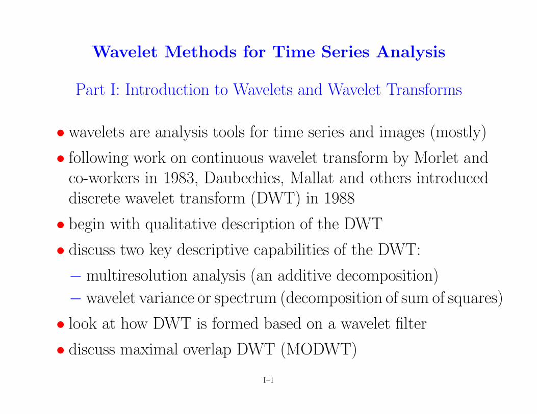
Wavelet Methods for Time Series Analysis

Part I: Introduction to Wavelets and Wavelet Transforms

• wavelets are analysis tools for time series and images (mostly)

• following work on continuous wavelet transform by Morlet andco-workers in 1983, Daubechies, Mallat and others introduceddiscrete wavelet transform (DWT) in 1988

• begin with qualitative description of the DWT

• discuss two key descriptive capabilities of the DWT:

− multiresolution analysis (an additive decomposition)

− wavelet variance or spectrum (decomposition of sum of squares)

• look at how DWT is formed based on a wavelet filter

• discuss maximal overlap DWT (MODWT)

I–1

Qualitative Description of DWT

• let X = [X0, X1, . . . , XN−1]T be a vector of N time series

values (note: ‘T ’ denotes transpose; i.e., X is a column vector)

• assume initially N = 2J for some positive integer J (will relaxthis restriction later on)

• DWT is a linear transform of X yielding N DWT coefficients

• notation: W = WX

−W is vector of DWT coefficients (jth component is Wj)

−W is N ×N orthonormal transform matrix

• orthonormality says WTW = IN (N ×N identity matrix)

• inverse of W is just its transpose, so WWT = IN also

WMTSA: 57, 53 I–2

Implications of Orthonormality

• let WTj• denote the jth row of W , where j = 0, 1, . . . , N − 1

• let Wj,l denote lth element of Wj•

• consider two rows, say, WTj• and WT

k•• orthonormality says

hWj•,Wk•i ≡N−1X

l=0

Wj,lWk,l =

(1, when j = k,

0, when j 6= k

− hWj•,Wk•i is inner product of jth & kth rows

− hWj•,Wj•i = kWj•k2 is squared norm (energy) for Wj•

WMTSA: 57, 42 I–3

Example: the Haar DWT

•N = 16 example of Haar DWT matrix W

................................................................................

................

................................

................

................

................

................

................

................

................................0

1

23

4

5

6

7

8

9

1011

12

13

14

15

0 5 10 15t

0 5 10 15t

• note that rows are orthogonal to each other

WMTSA: 57 I–4

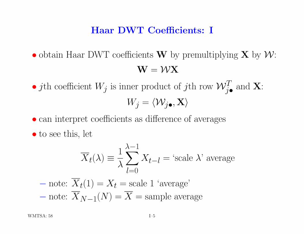
Haar DWT Coefficients: I

• obtain Haar DWT coefficients W by premultiplying X by W :

W = WX

• jth coefficient Wj is inner product of jth row WTj• and X:

Wj = hWj•,Xi

• can interpret coefficients as difference of averages

• to see this, let

Xt(λ) ≡ 1

λ

λ−1X

l=0

Xt−l = ‘scale λ’ average

− note: Xt(1) = Xt = scale 1 ‘average’

− note: XN−1(N) = X = sample average

WMTSA: 58 I–5

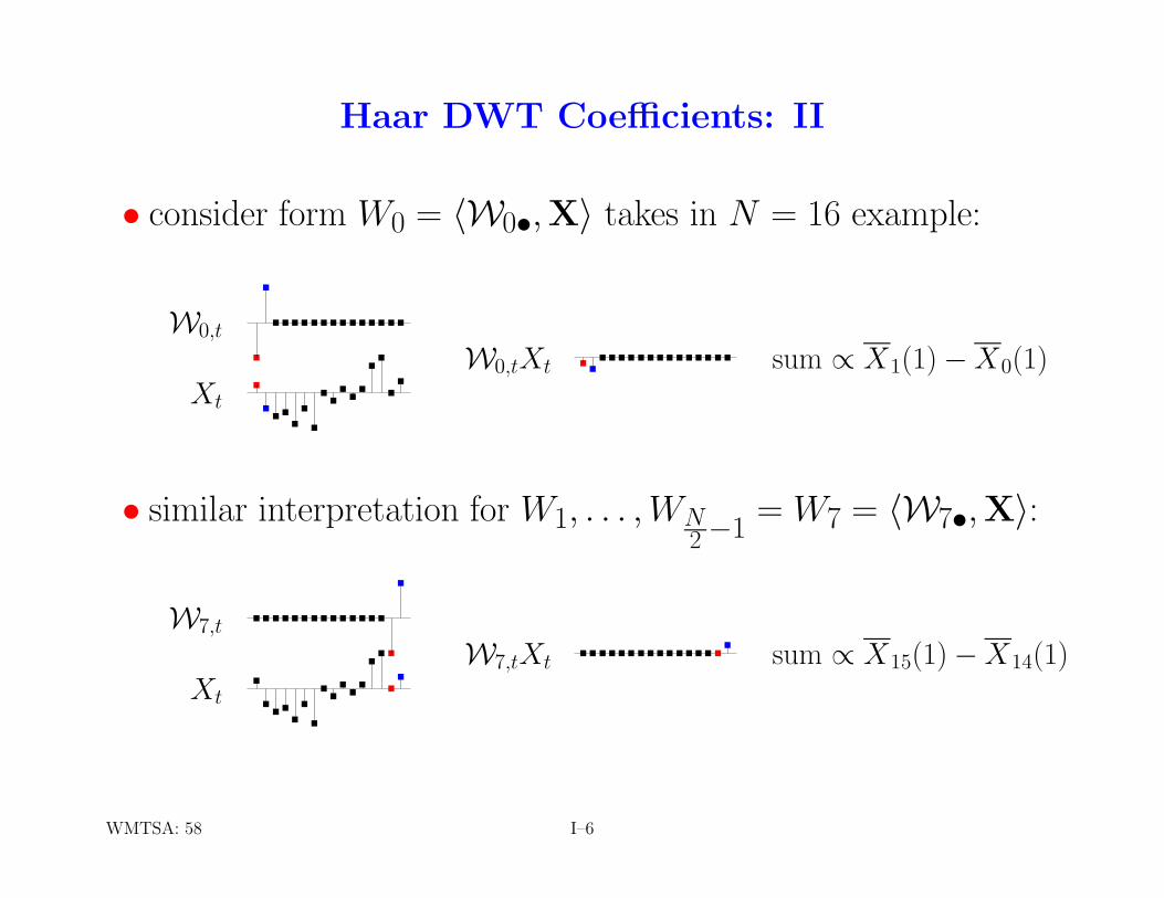
Haar DWT Coefficients: II

• consider form W0 = hW0•,Xi takes in N = 16 example:

............................

.... ................W0,t

Xt

W0,tXt sum ∝ X1(1)−X0(1)

• similar interpretation for W1, . . . ,WN2 −1

= W7 = hW7•,Xi:

................................ ................W7,t

Xt

W7,tXt sum ∝ X15(1)−X14(1)

WMTSA: 58 I–6

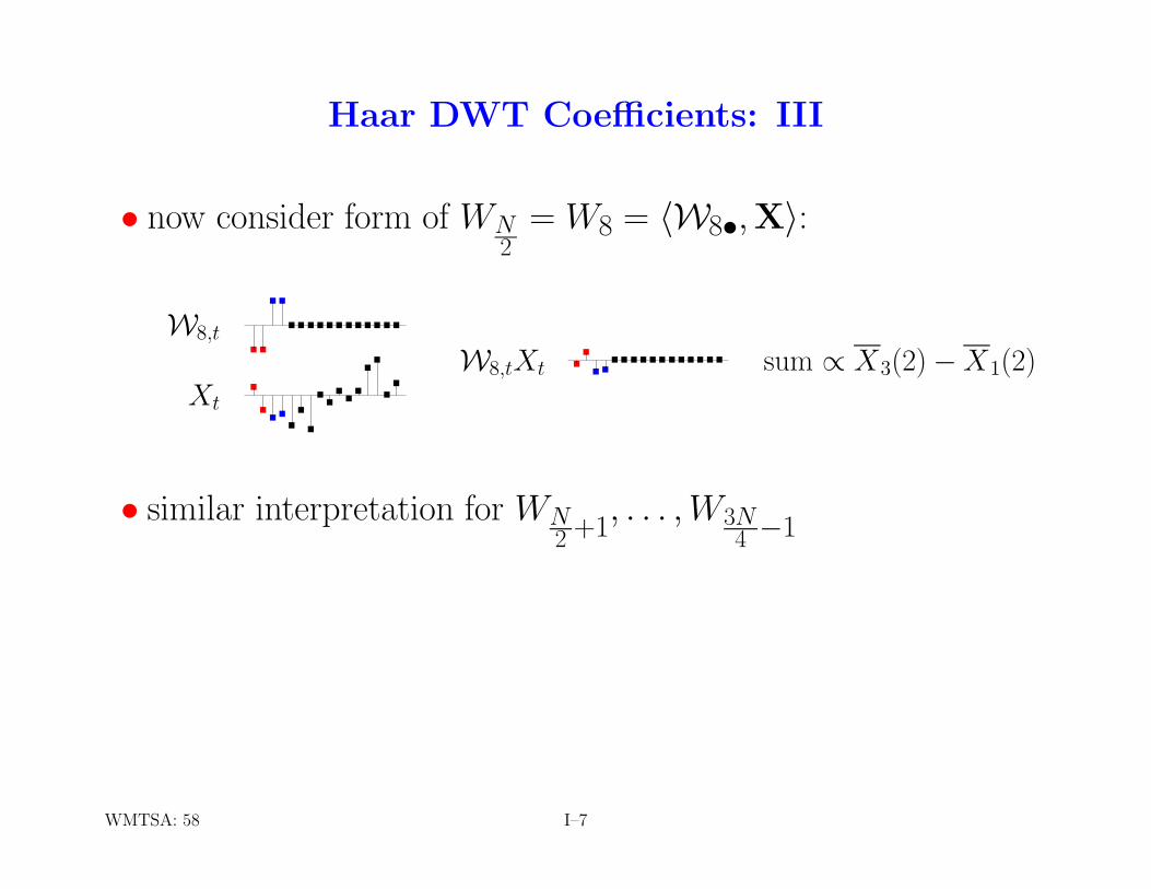
Haar DWT Coefficients: III

• now consider form of WN2

= W8 = hW8•,Xi:

....................

........................

....W8,t

Xt

W8,tXt sum ∝ X3(2)−X1(2)

• similar interpretation for WN2 +1

, . . . ,W3N4 −1

WMTSA: 58 I–7

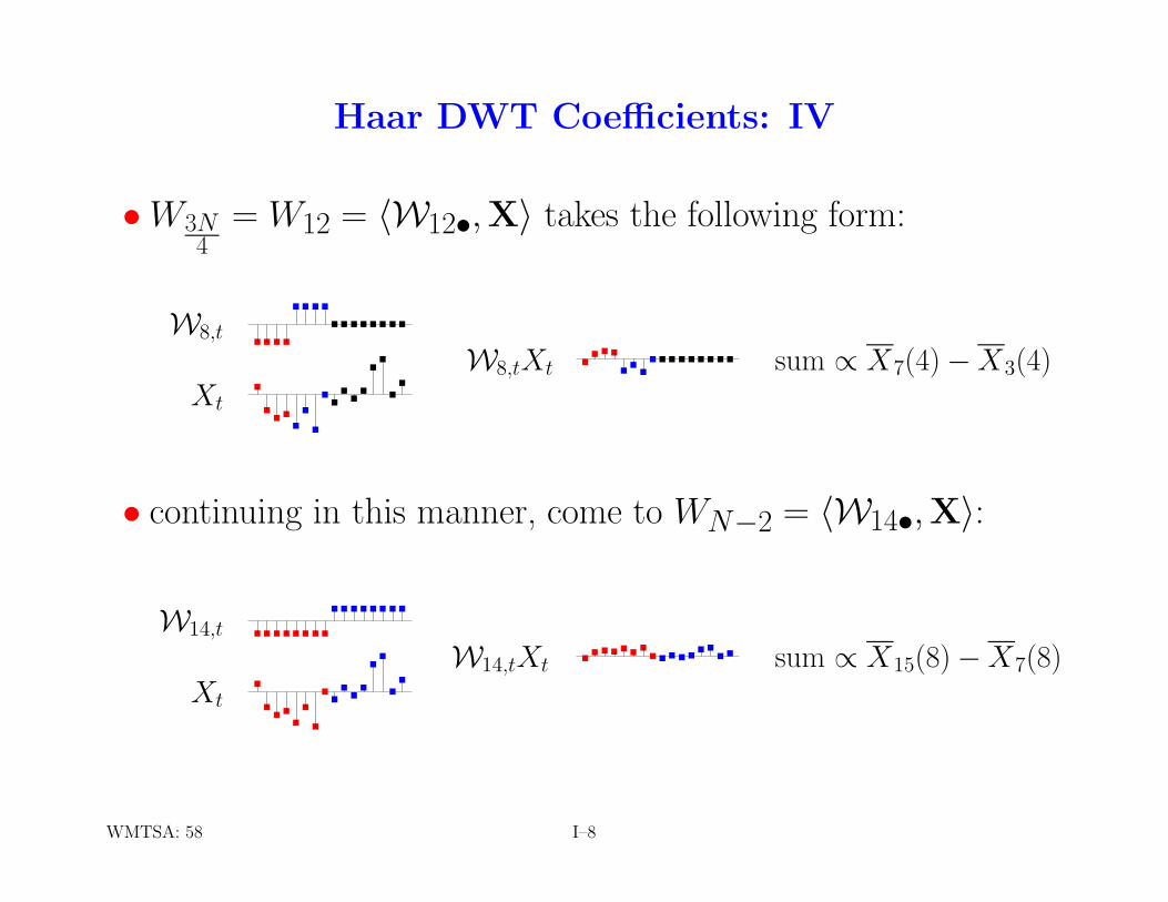
Haar DWT Coefficients: IV

•W3N4

= W12 = hW12•,Xi takes the following form:

................

................ ................W8,t

Xt

W8,tXt sum ∝ X7(4)−X3(4)

• continuing in this manner, come to WN−2 = hW14•,Xi:

................

................ ................W14,t

Xt

W14,tXt sum ∝ X15(8)−X7(8)

WMTSA: 58 I–8

Haar DWT Coefficients: V

• final coefficient WN−1 = W15 has a different interpretation:

................

................ ................W15,t

Xt

W15,tXt sum ∝ X15(16)

• structure of rows in W− first N

2 rows yield Wj’s ∝ changes on scale 1

− next N4 rows yield Wj’s ∝ changes on scale 2

− next N8 rows yield Wj’s ∝ changes on scale 4

− next to last row yields Wj ∝ change on scale N2

− last row yields Wj ∝ average on scale N

WMTSA: 58–59 I–9

Structure of DWT Matrices

• N2τj

wavelet coefficients for scale τj ≡ 2j−1, j = 1, . . . , J

− τj ≡ 2j−1 is standardized scale

− τj ∆ is physical scale, where ∆ is sampling interval

• each Wj localized in time: as scale ↑, localization ↓• rows of W for given scale τj:

− circularly shifted with respect to each other

− shift between adjacent rows is 2τj = 2j

• similar structure for DWTs other than the Haar

• differences of averages common theme for DWTs

− simple differencing replaced by higher order differences

− simple averages replaced by weighted averages

WMTSA: 59–61 I–10

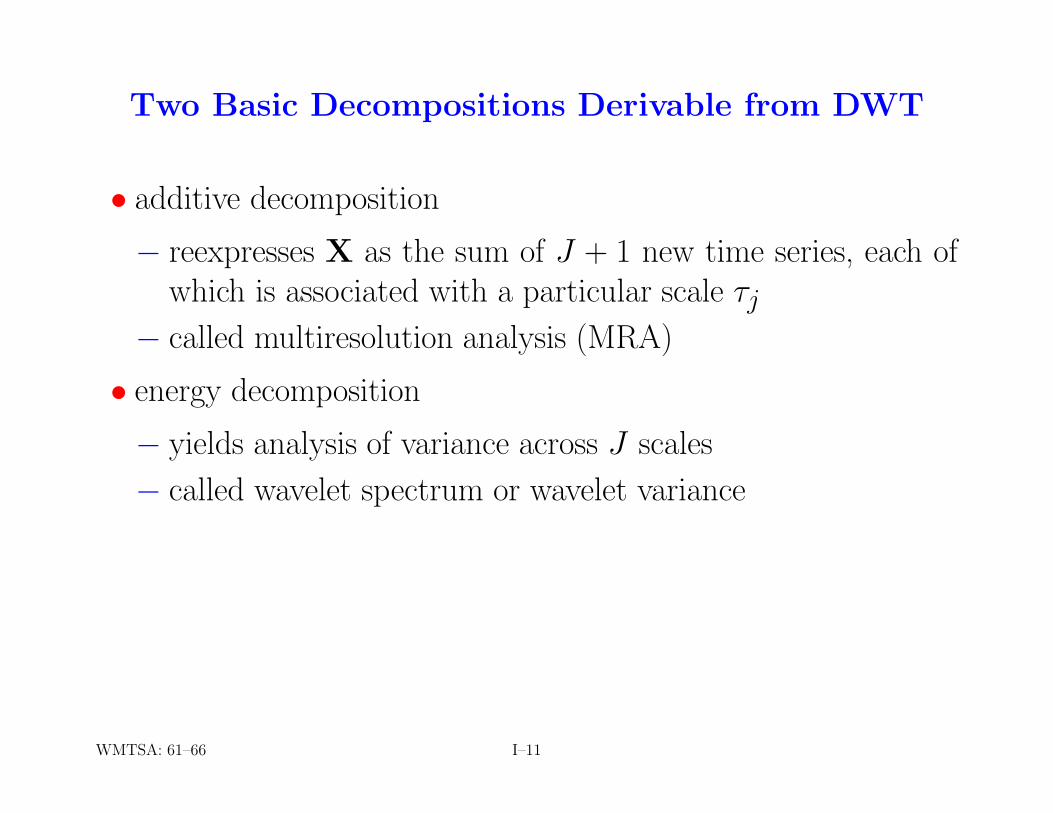
Two Basic Decompositions Derivable from DWT

• additive decomposition

− reexpresses X as the sum of J + 1 new time series, each ofwhich is associated with a particular scale τj

− called multiresolution analysis (MRA)

• energy decomposition

− yields analysis of variance across J scales

− called wavelet spectrum or wavelet variance

WMTSA: 61–66 I–11

Partitioning of DWT Coefficient Vector W

• decompositions are based on partitioning of W and W• partition W into subvectors associated with scale:

W =

W1W2

...Wj

...WJVJ

•Wj has N/2j elements (scale τj = 2j−1 changes)

note:PJ

j=1N2j = N

2 + N4 + · · · + 2 + 1 = 2J − 1 = N − 1

•VJ has 1 element, which is equal to√

N ·X (scale N average)

WMTSA: 61–62 I–12

Example of Partitioning of W

• consider time series X of length N = 16 & its Haar DWT W

. . . . . . . . . ... . . .

.

. . . . . . . . . . . . . . . .

W1 W2 W3 W4 V4

W

X

2

0

−22

0

−20 5 10 15

t

WMTSA: 62, 42 I–13

Partitioning of DWT Matrix W

• partition W commensurate with partitioning of W:

W =

W1W2...Wj...

WJVJ

• Wj is N2j ×N matrix (related to scale τj = 2j−1 changes)

• VJ is 1×N row vector (each element is 1√N

)

WMTSA: 63 I–14

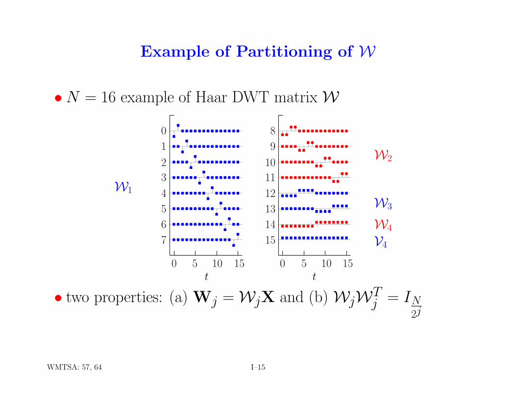
Example of Partitioning of W

•N = 16 example of Haar DWT matrix W

................................................................................

................

................................

................

................

................

................

................

................

................................

W1

W2

W3

W4

V4

0

1

23

4

5

6

7

8

9

1011

12

13

14

15

0 5 10 15t

0 5 10 15t

• two properties: (a) Wj = WjX and (b) WjWTj = IN

2j

WMTSA: 57, 64 I–15

DWT Analysis and Synthesis Equations

• recall the DWT analysis equation W = WX

• WTW = IN because W is an orthonormal transform

• implies that WTW = WTWX = X

• yields DWT synthesis equation:

X = WTW =hWT

1 ,WT2 , . . . ,WT

J ,VTJ

i

W1W2

...WJVJ

=JX

j=1

WTj Wj + VT

J VJ

WMTSA: 63 I–16

Multiresolution Analysis: I

• synthesis equation leads to additive decomposition:

X =JX

j=1

WTj Wj + VT

J VJ ≡JX

j=1

Dj + SJ

• Dj ≡WTj Wj is portion of synthesis due to scale τj

• Dj is vector of length N and is called jth ‘detail’

• SJ ≡ VTJ VJ = X1, where 1 is a vector containing N ones

(later on we will call this the ‘smooth’ of Jth order)

• additive decomposition called multiresolution analysis (MRA)

WMTSA: 64–65 I–17

Multiresolution Analysis: II

• example of MRA for time series of length N = 16

...............

...............

..............................

...............

..

.

..

.............

...

S4

D4

D3

D2

D1

X10

−10 5 10 15

t

• adding values for, e.g., t = 14 in D1, . . . ,D4 & S4 yields X14

WMTSA: 64 I–18

Energy Preservation Property of DWT Coefficients

• define ‘energy’ in X as its squared norm:

kXk2 = hX,Xi = XTX =N−1X

t=0

X2t

• energy of X is preserved in its DWT coefficients W because

kWk2 = WTW = (WX)TWX

= XTWTWX= XTINX = XTX = kXk2

• note: same argument holds for any orthonormal transform

WMTSA: 43 I–19

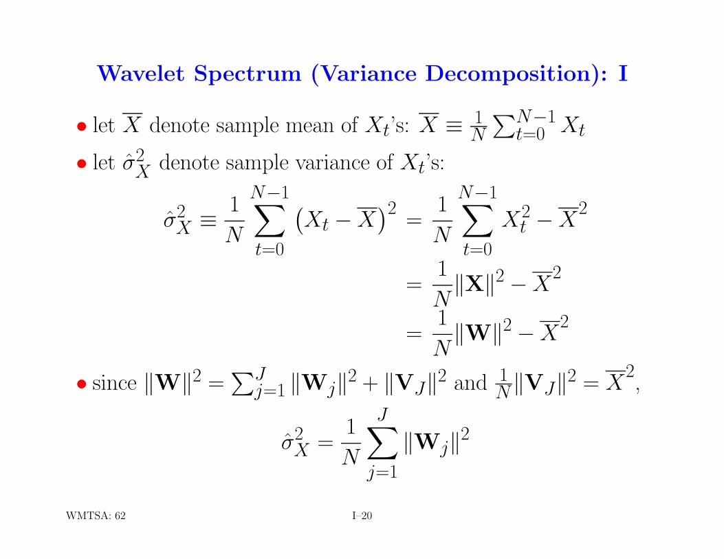
Wavelet Spectrum (Variance Decomposition): I

• let X denote sample mean of Xt’s: X ≡ 1N

PN−1t=0 Xt

• let σ2X denote sample variance of Xt’s:

σ2X ≡ 1

N

N−1X

t=0

°Xt −X

¢2=

1

N

N−1X

t=0

X2t −X

2

=1

NkXk2 −X

2

=1

NkWk2 −X

2

• since kWk2 =PJ

j=1 kWjk2 + kVJk2 and 1NkVJk2 = X

2,

σ2X =

1

N

JX

j=1

kWjk2

WMTSA: 62 I–20

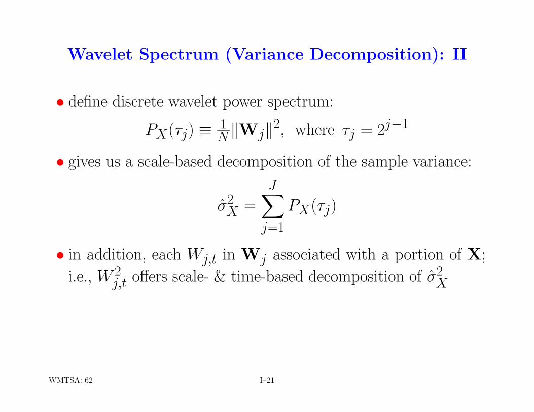
Wavelet Spectrum (Variance Decomposition): II

• define discrete wavelet power spectrum:

PX(τj) ≡ 1NkWjk2, where τj = 2j−1

• gives us a scale-based decomposition of the sample variance:

σ2X =

JX

j=1

PX(τj)

• in addition, each Wj,t in Wj associated with a portion of X;i.e., W 2

j,t offers scale- & time-based decomposition of σ2X

WMTSA: 62 I–21

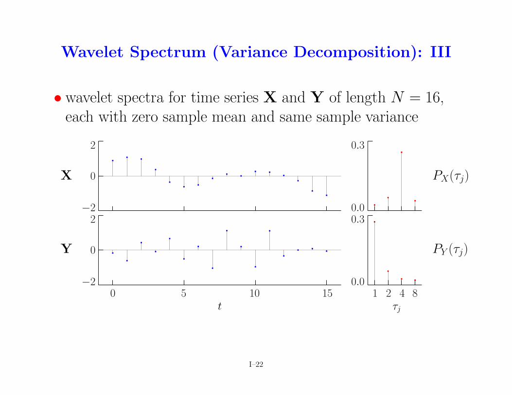
Wavelet Spectrum (Variance Decomposition): III

• wavelet spectra for time series X and Y of length N = 16,each with zero sample mean and same sample variance

. . ..

. . . . . . . . . .. .

. .. .

..

..

..

.

.

. . . .

. .

.

.

.

. . .

X

Y

PX(τj)

PY (τj)

2

0

−22

0

−2

0.3

0.00.3

0.00 5 10 15 1 2 4 8

t τj

I–22

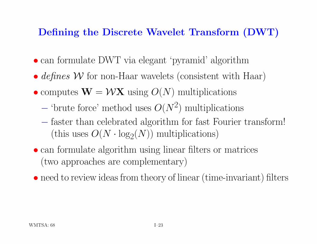
Defining the Discrete Wavelet Transform (DWT)

• can formulate DWT via elegant ‘pyramid’ algorithm

• defines W for non-Haar wavelets (consistent with Haar)

• computes W = WX using O(N) multiplications

− ‘brute force’ method uses O(N2) multiplications

− faster than celebrated algorithm for fast Fourier transform!(this uses O(N · log2(N)) multiplications)

• can formulate algorithm using linear filters or matrices(two approaches are complementary)

• need to review ideas from theory of linear (time-invariant) filters

WMTSA: 68 I–23

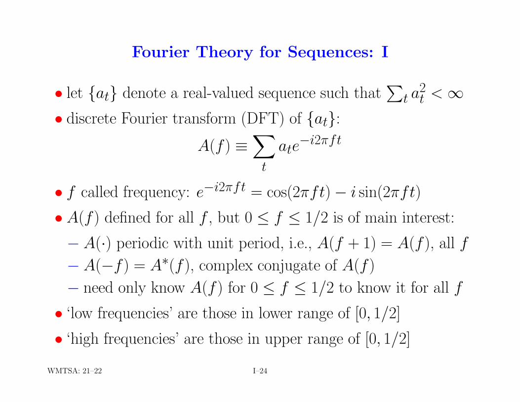
Fourier Theory for Sequences: I

• let {at} denote a real-valued sequence such thatP

t a2t < ∞

• discrete Fourier transform (DFT) of {at}:A(f) ≡

X

t

ate−i2πft

• f called frequency: e−i2πft = cos(2πft)− i sin(2πft)

• A(f) defined for all f , but 0 ≤ f ≤ 1/2 is of main interest:

− A(·) periodic with unit period, i.e., A(f + 1) = A(f), all f

− A(−f) = A∗(f), complex conjugate of A(f)

− need only know A(f) for 0 ≤ f ≤ 1/2 to know it for all f

• ‘low frequencies’ are those in lower range of [0, 1/2]

• ‘high frequencies’ are those in upper range of [0, 1/2]

WMTSA: 21–22 I–24

Fourier Theory for Sequences: II

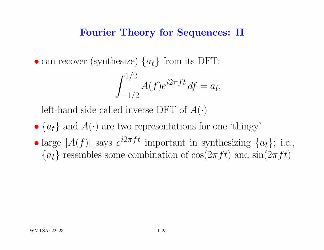
• can recover (synthesize) {at} from its DFT:Z 1/2

−1/2A(f)ei2πft df = at;

left-hand side called inverse DFT of A(·)• {at} and A(·) are two representations for one ‘thingy’

• large |A(f)| says ei2πft important in synthesizing {at}; i.e.,{at} resembles some combination of cos(2πft) and sin(2πft)

WMTSA: 22–23 I–25

Convolution of Sequences

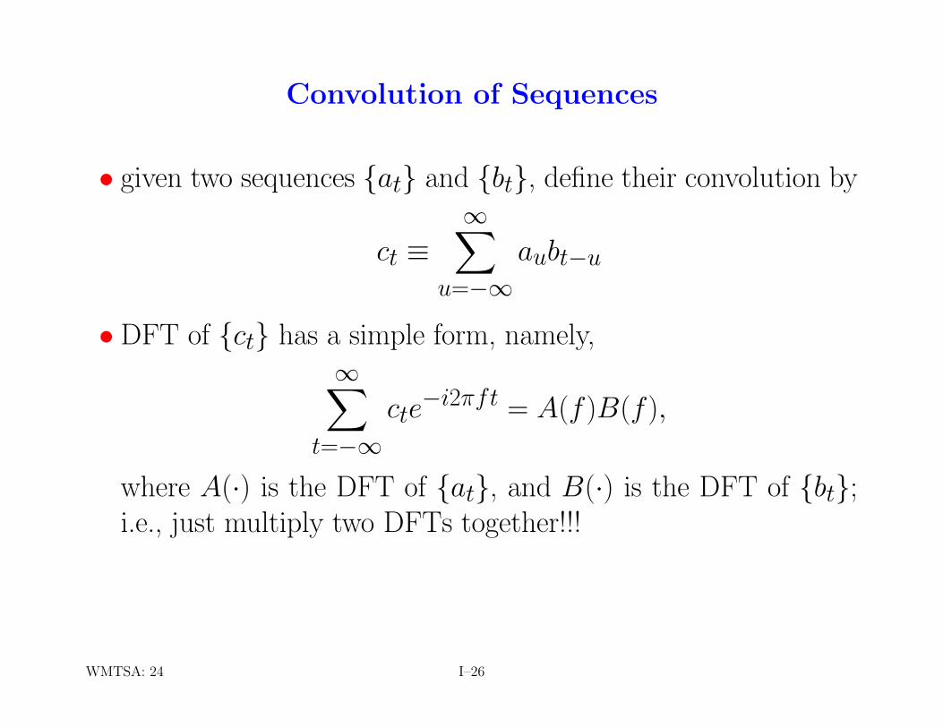
• given two sequences {at} and {bt}, define their convolution by

ct ≡∞X

u=−∞aubt−u

• DFT of {ct} has a simple form, namely,∞X

t=−∞cte

−i2πft = A(f)B(f),

where A(·) is the DFT of {at}, and B(·) is the DFT of {bt};i.e., just multiply two DFTs together!!!

WMTSA: 24 I–26

Basic Concepts of Filtering

• convolution & linear time-invariant filtering are same concepts:

− {bt} is input to filter

− {at} represents the filter

− {ct} is filter output

• flow diagram for filtering: {bt} −→ {at} −→ {ct}• {at} is called impulse response sequence for filter

• its DFT A(·) is called transfer function

• in general A(·) is complex-valued, so write A(f) = |A(f)|eiθ(f)

− |A(f)| defines gain function

−A(f) ≡ |A(f)|2 defines squared gain function

− θ(·) called phase function (well-defined at f if |A(f)| > 0)

WMTSA: 25 I–27

Example of a Low-Pass Filter

• consider bt = 316

≥45

¥|t|+ 1

20

≥−4

5

¥|t|& at =

12, t = 014, t = −1 or 1

0, otherwise

.................

................. .................{bt} {at} {ct}

B(·) A(·) A(·)B(·)−8 −4 0 4 8 −8 −4 0 4 8 −8 −4 0 4 8

t t t

0

2

1

00.0 0.5 0.0 0.50.0 0.5

f f f

• note: A(·) & B(·) both real-valued (A(·) = its gain function)

WMTSA: 25–26 I–28

Example of a High-Pass Filter

• consider same {bt}, but now let at =

12, t = 0

−14, t = −1 or 1

0, otherwise

.................

................. .................{bt} {at} {ct}

B(·) A(·) A(·)B(·)−8 −4 0 4 8 −8 −4 0 4 8 −8 −4 0 4 8

t t t

0

2

1

00.0 0.5 0.0 0.50.0 0.5

f f f

• note: {at} resembles some wavelet filters we’ll see later

WMTSA: 26–27 I–29

The Wavelet Filter: I

• precise definition of DWT begins with notion of wavelet filter

• let {hl : l = 0, . . . , L− 1} be a real-valued filter of width L

− both h0 and hL−1 must be nonzero

− for convenience, will define hl = 0 for l < 0 and l ≥ L

− L must be even (2, 4, 6, 8, . . .) for technical reasons (henceruling out {at} on the previous overhead)

WMTSA: 26–27 I–30

The Wavelet Filter: II

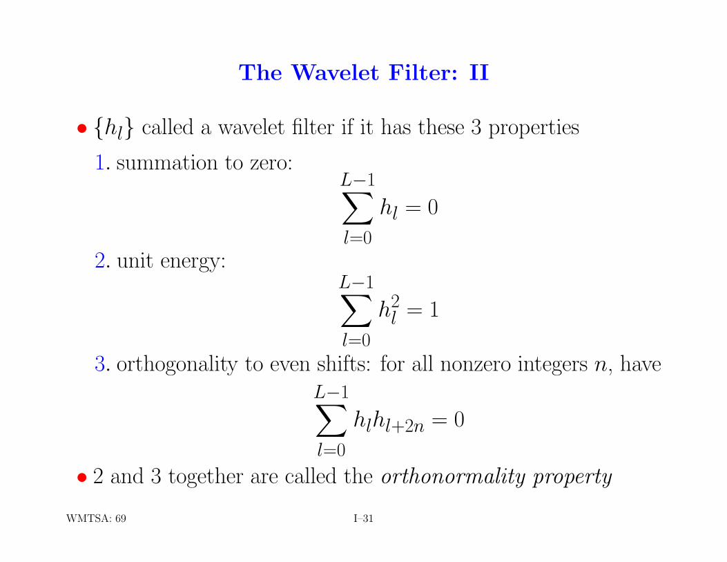
• {hl} called a wavelet filter if it has these 3 properties

1. summation to zero:L−1X

l=0

hl = 0

2. unit energy:L−1X

l=0

h2l = 1

3. orthogonality to even shifts: for all nonzero integers n, haveL−1X

l=0

hlhl+2n = 0

• 2 and 3 together are called the orthonormality property

WMTSA: 69 I–31

The Wavelet Filter: III

• summation to zero and unit energy relatively easy to achieve

• orthogonality to even shifts is key property & hardest to satisfy

• define transfer and squared gain functions for wavelet filter:

H(f) ≡L−1X

l=0

hle−i2πfl and H(f) ≡ |H(f)|2

• orthonormality property is equivalent to

H(f) +H(f + 12) = 2 for all f

(an elegant – but not obvious! – result)

WMTSA: 69–70 I–32

Haar Wavelet Filter

• simplest wavelet filter is Haar (L = 2): h0 = 1√2 & h1 = − 1√

2

• note that h0 + h1 = 0 and h20 + h2

1 = 1, as required

• orthogonality to even shifts also readily apparent

................................

................hl

hl−2

hlhl−2 sum = 0

WMTSA: 69–70 I–33

D(4) Wavelet Filter: I

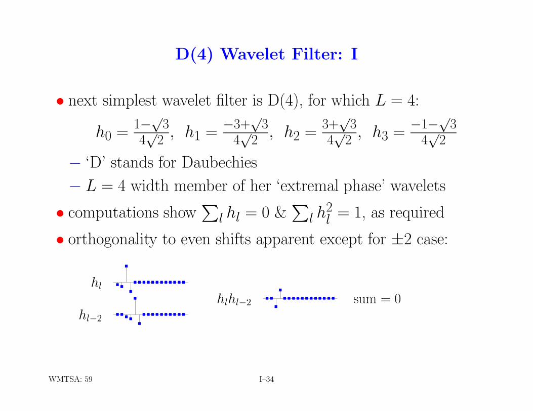
• next simplest wavelet filter is D(4), for which L = 4:

h0 = 1−√

34√

2 , h1 = −3+√

34√

2 , h2 = 3+√

34√

2 , h3 = −1−√

34√

2

− ‘D’ stands for Daubechies

− L = 4 width member of her ‘extremal phase’ wavelets

• computations showP

l hl = 0 &P

l h2l = 1, as required

• orthogonality to even shifts apparent except for ±2 case:

................................

................hl

hl−2

hlhl−2 sum = 0

WMTSA: 59 I–34

D(4) Wavelet Filter: II

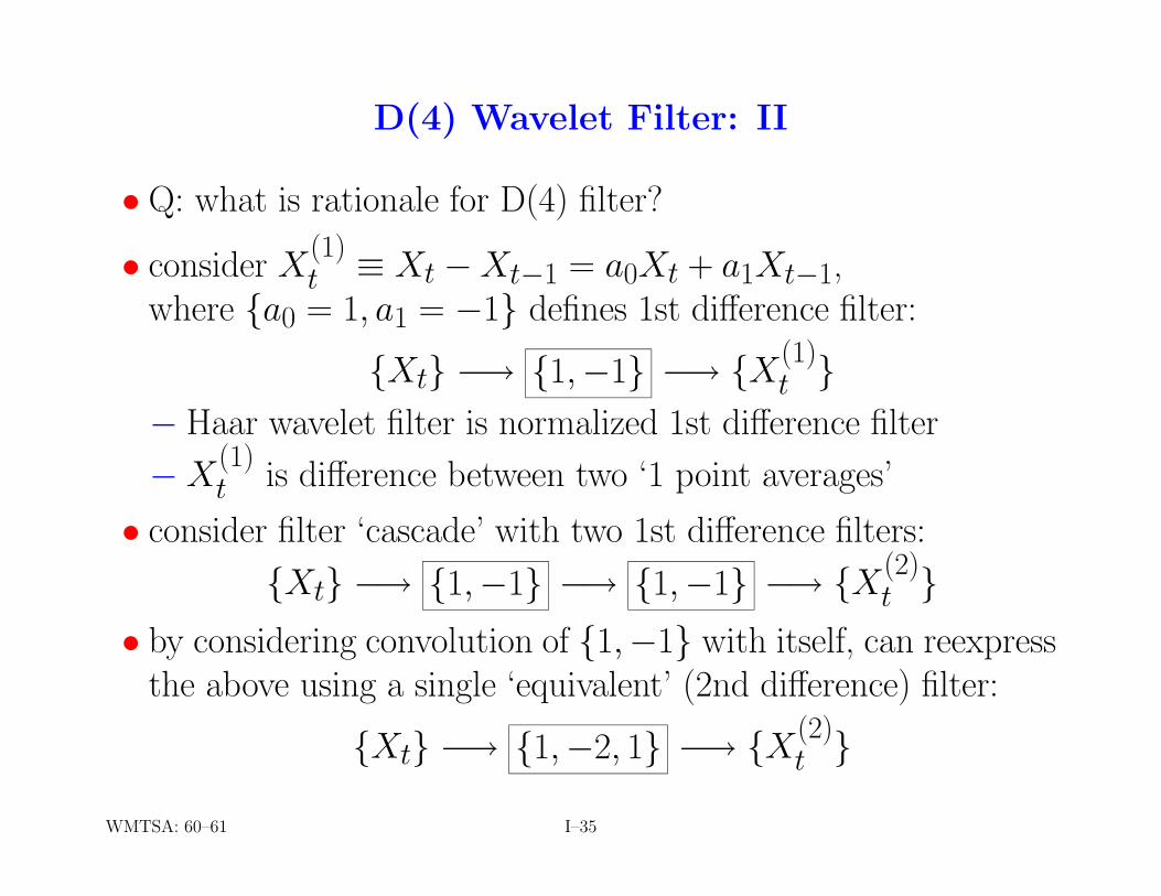
• Q: what is rationale for D(4) filter?

• consider X(1)t ≡ Xt −Xt−1 = a0Xt + a1Xt−1,

where {a0 = 1, a1 = −1} defines 1st difference filter:

{Xt} −→ {1,−1} −→ {X(1)t }

− Haar wavelet filter is normalized 1st difference filter

−X(1)t is difference between two ‘1 point averages’

• consider filter ‘cascade’ with two 1st difference filters:

{Xt} −→ {1,−1} −→ {1,−1} −→ {X(2)t }

• by considering convolution of {1,−1} with itself, can reexpressthe above using a single ‘equivalent’ (2nd difference) filter:

{Xt} −→ {1,−2, 1} −→ {X(2)t }

WMTSA: 60–61 I–35

D(4) Wavelet Filter: III

• renormalizing and shifting 2nd difference filter yields high-passfilter considered earlier:

at =

12, t = 0

−14, t = −1 or 1

0, otherwise

• consider ‘2 point weighted average’ followed by 2nd difference:

{Xt} −→ {a, b} −→ {1,−2, 1} −→ {Yt}

• convolution of {a, b} and {1,−2, 1} yields an equivalent filter,which is how the D(4) wavelet filter arises:

{Xt} −→ {h0, h1, h2, h3} −→ {Yt}

WMTSA: 60–61 I–36

D(4) Wavelet Filter: IV

• using conditions

1. summation to zero: h0 + h1 + h2 + h3 = 0

2. unit energy: h20 + h2

1 + h22 + h2

3 = 1

3. orthogonality to even shifts: h0h2 + h1h3 = 0

can solve for feasible values of a and b

• one solution is a = 1+√

34√

2.= 0.48 and b = −1+

√3

4√

2.= 0.13

(other solutions yield essentially the same filter)

• interpret D(4) filtered output as changes in weighted averages

− ‘change’ now measured by 2nd difference (1st for Haar)

− average is now 2 point weighted average (1 point for Haar)

− can argue that effective scale of weighted average is one

WMTSA: 60–61 I–37

Another Popular Daubechies Wavelet Filter

• LA(8) wavelet filter (‘LA’ stands for ‘least asymmetric’)

................

................

................

................

................

................

................

hl

hl−2

hl−4

hl−6

hlhl−2 sum = 0

hlhl−4 sum = 0

hlhl−6 sum = 0

• resembles three-point high-pass filter {−14,

12,−

14} (somewhat)

• can interpret this filter as cascade consisting of

− 4th difference filter

− weighted average filter of width 4, but effective width 1

• filter output can be interpreted as changes in weighted averages

WMTSA: 108–109 I–38

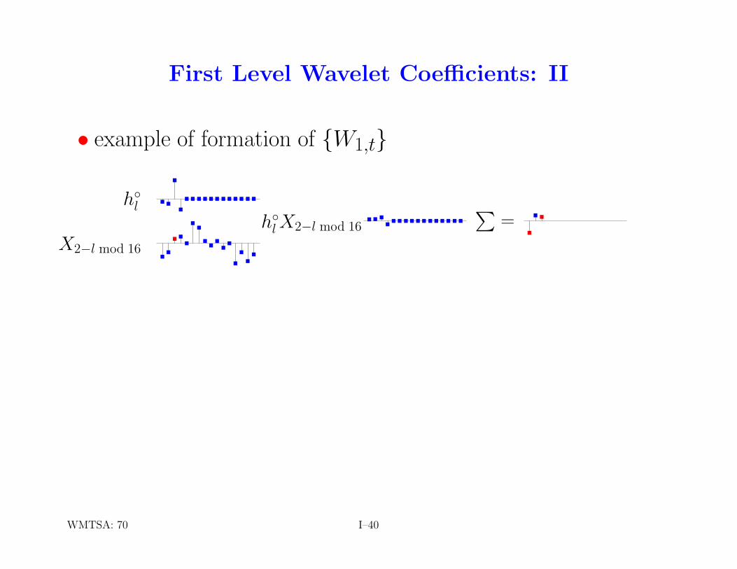
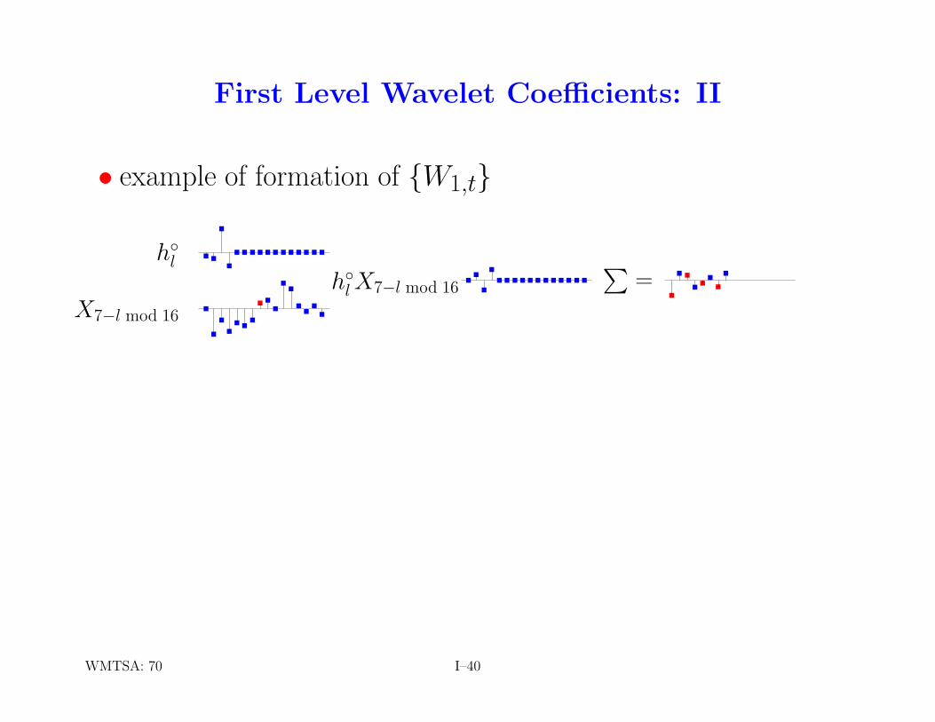
First Level Wavelet Coefficients: I

• given wavelet filter {hl} of width L & time series of lengthN = 2J , obtain first level wavelet coefficients as follows

• circularly filter X with wavelet filter to yield outputL−1X

l=0

hlXt−l =L−1X

l=0

hlXt−l mod N, t = 0, . . . , N − 1;

i.e., if t− l does not satisfy 0 ≤ t− l ≤ N − 1, interpret Xt−las Xt−l mod N ; e.g., X−1 = XN−1 and X−2 = XN−2

• take every other value of filter output to define

W1,t ≡L−1X

l=0

hlX2t+1−l mod N, t = 0, . . . , N2 − 1;

{W1,t} formed by downsampling filter output by a factor of 2

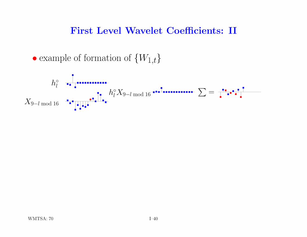
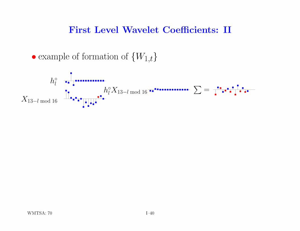
WMTSA: 70 I–39

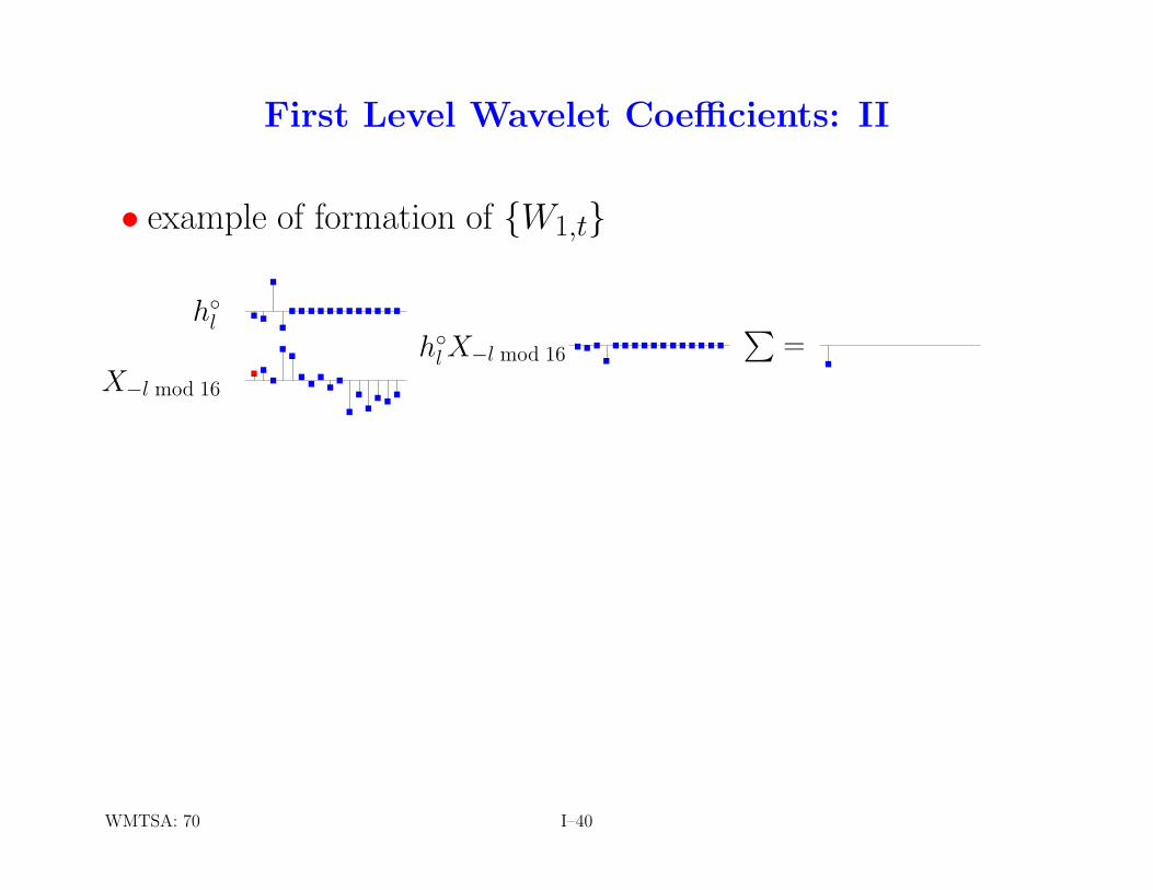
First Level Wavelet Coefficients: II

• example of formation of {W1,t}

................

................................ .

h◦l

X−l mod 16

h◦l X−l mod 16

P=

WMTSA: 70 I–40



................................

................ ..h◦l

X1−l mod 16

h◦l X1−l mod 16

P=

WMTSA: 70 I–40



................................

................ ...h◦l

X2−l mod 16

h◦l X2−l mod 16

P=

WMTSA: 70 I–40



................................

................ ....h◦l

X3−l mod 16

h◦l X3−l mod 16

P=

WMTSA: 70 I–40



................................

................ .....h◦l

X4−l mod 16

h◦l X4−l mod 16

P=

WMTSA: 70 I–40



................................

................ ......h◦l

X5−l mod 16

h◦l X5−l mod 16

P=

WMTSA: 70 I–40



................................

................ .......h◦l

X6−l mod 16

h◦l X6−l mod 16

P=

WMTSA: 70 I–40



................................

................ ........h◦l

X7−l mod 16

h◦l X7−l mod 16

P=

WMTSA: 70 I–40



................................ ................ .........h◦l

X8−l mod 16

h◦l X8−l mod 16

P=

WMTSA: 70 I–40



................................ ................ ..........h◦l

X9−l mod 16

h◦l X9−l mod 16

P=

WMTSA: 70 I–40



................................ ................ ...........h◦l

X10−l mod 16

h◦l X10−l mod 16

P=

WMTSA: 70 I–40



................................ ................ ............h◦l

X11−l mod 16


P=

WMTSA: 70 I–40



................................ ................ .............h◦l

X12−l mod 16


P=

WMTSA: 70 I–40



................................ ................ ..............h◦l

X13−l mod 16


P=

WMTSA: 70 I–40



................................ ................ ...............h◦l

X14−l mod 16


P=

WMTSA: 70 I–40



................................

................ ................h◦l

X15−l mod 16


P=

WMTSA: 70 I–40



................................

................ ................h◦l

X15−l mod 16


P=

........↓ 2

W1,t

• {W1,t} are unit scale wavelet coefficients – these are the ele-ments of W1 and first N/2 elements of W = WX

• also have W1 = W1X, with W1 being first N/2 rows of W• hence elements of W1 dictated by wavelet filter

WMTSA: 70 I–40

Upper Half W1 of Haar DWT Matrix W

• consider Haar wavelet filter (L = 2): h0 = 1√2 & h1 = − 1√

2

• when N = 16, W1 looks like

h1 h0 0 0 0 0 0 0 0 0 0 0 0 0 0 00 0 h1 h0 0 0 0 0 0 0 0 0 0 0 0 00 0 0 0 h1 h0 0 0 0 0 0 0 0 0 0 00 0 0 0 0 0 h1 h0 0 0 0 0 0 0 0 00 0 0 0 0 0 0 0 h1 h0 0 0 0 0 0 00 0 0 0 0 0 0 0 0 0 h1 h0 0 0 0 00 0 0 0 0 0 0 0 0 0 0 0 h1 h0 0 00 0 0 0 0 0 0 0 0 0 0 0 0 0 h1 h0

• rows obviously orthogonal to each other

I–41

Upper Half W1 of D(4) DWT Matrix W

• when L = 4 & N = 16, W1 looks like

h1 h0 0 0 0 0 0 0 0 0 0 0 0 0 h3 h2h3 h2 h1 h0 0 0 0 0 0 0 0 0 0 0 0 00 0 h3 h2 h1 h0 0 0 0 0 0 0 0 0 0 00 0 0 0 h3 h2 h1 h0 0 0 0 0 0 0 0 00 0 0 0 0 0 h3 h2 h1 h0 0 0 0 0 0 00 0 0 0 0 0 0 0 h3 h2 h1 h0 0 0 0 00 0 0 0 0 0 0 0 0 0 h3 h2 h1 h0 0 00 0 0 0 0 0 0 0 0 0 0 0 h3 h2 h1 h0

• rows orthogonal because h0h2 + h1h3 = 0

• note: hW0•,Xi yields W0 = h1X0 + h0X1 + h3X14 + h2X15

• unlike other coefficients from above, this ‘boundary’ coefficientdepends on circular treatment of X (a curse, not a feature!)

WMTSA: 81 I–42

Orthonormality of Upper Half of DWT Matrix: I

• can show that, for all L and even N ,

W1,t =L−1X

l=0

hlX2t+1−l mod N, or, equivalently, W1 = W1X

forms half an orthonormal transform; i.e.,

W1WT1 = IN

2

• Q: how can we construct the other half of W?

WMTSA: 72 I–43

The Scaling Filter: I

• create scaling (or ‘father wavelet’) filter {gl} by reversing {hl}and then changing sign of coefficients with even indices

.. .

. ..

.... ..

..

....

........ .

....... .

.......

{hl} {hl} reversed {gl}

Haar

D(4)

LA(8)

• 2 filters related by gl ≡ (−1)l+1hL−1−l & hl = (−1)lgL−1−l

WMTSA: 75 I–44

The Scaling Filter: II

• {gl} is ‘quadrature mirror’ filter corresponding to {hl}• properties 2 and 3 of {hl} are shared by {gl}:

2. unit energy:L−1X

l=0

g2l = 1

3. orthogonality to even shifts: for all nonzero integers n, have

L−1X

l=0

glgl+2n = 0

• scaling & wavelet filters both satisfy orthonormality property

WMTSA: 76 I–45

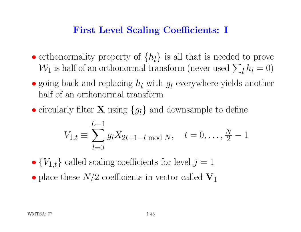
First Level Scaling Coefficients: I

• orthonormality property of {hl} is all that is needed to proveW1 is half of an orthonormal transform (never used

Pl hl = 0)

• going back and replacing hl with gl everywhere yields anotherhalf of an orthonormal transform

• circularly filter X using {gl} and downsample to define

V1,t ≡L−1X

l=0

glX2t+1−l mod N, t = 0, . . . , N2 − 1

• {V1,t} called scaling coefficients for level j = 1

• place these N/2 coefficients in vector called V1

WMTSA: 77 I–46

First Level Scaling Coefficients: III

• define V1 in a manner analogous to W1 so that V1 = V1X

• when L = 4 and N = 16, V1 looks like

g1 g0 0 0 0 0 0 0 0 0 0 0 0 0 g3 g2g3 g2 g1 g0 0 0 0 0 0 0 0 0 0 0 0 00 0 g3 g2 g1 g0 0 0 0 0 0 0 0 0 0 00 0 0 0 g3 g2 g1 g0 0 0 0 0 0 0 0 00 0 0 0 0 0 g3 g2 g1 g0 0 0 0 0 0 00 0 0 0 0 0 0 0 g3 g2 g1 g0 0 0 0 00 0 0 0 0 0 0 0 0 0 g3 g2 g1 g0 0 00 0 0 0 0 0 0 0 0 0 0 0 g3 g2 g1 g0

• V1 obeys same orthonormality property as W1:

similar to W1WT1 = IN

2, have V1VT

1 = IN2

WMTSA: 77 I–47

Orthonormality of V1 and W1: I

• Q: how does V1 help us?

• A: rows of V1 and W1 are pairwise orthogonal!

• readily apparent in Haar case:

................................

................

gl

hl

glhl sum = 0

WMTSA: 77–78 I–48

Orthonormality of V1 and W1: II

• let’s check that orthogonality holds for D(4) case also:

................

................

................

................

................gl

hl

hl−2

glhl sum = 0

glhl−2 sum = 0

I–49

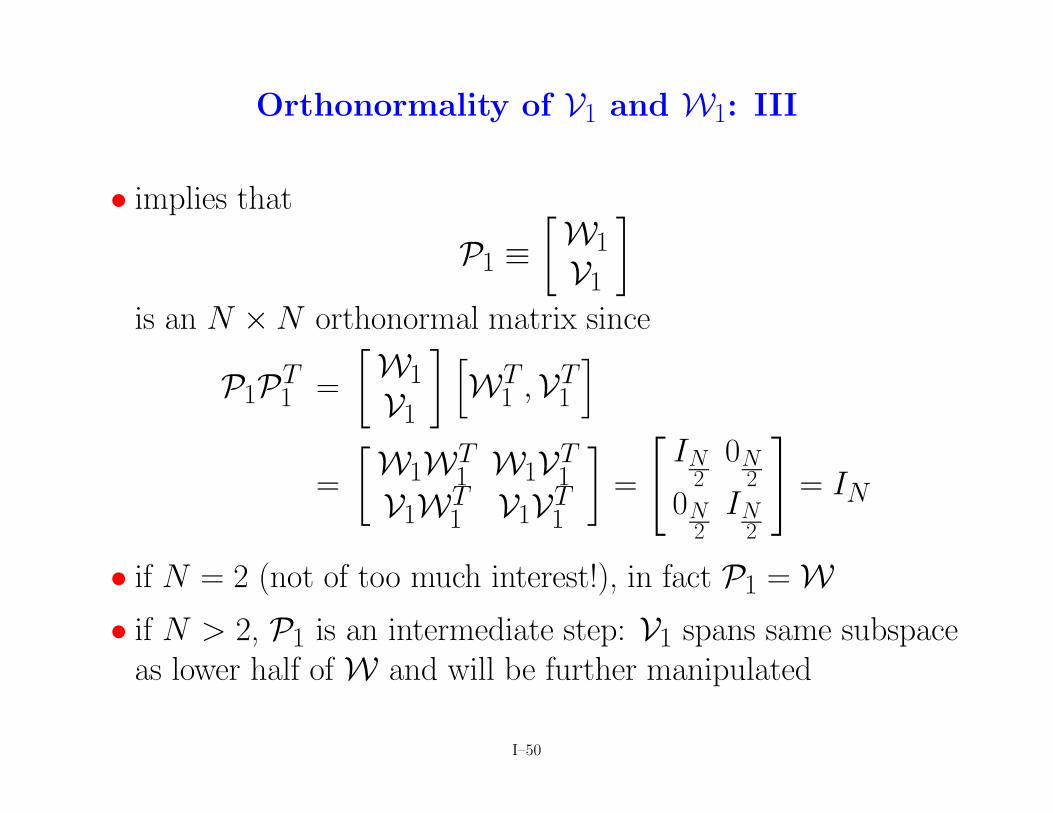
Orthonormality of V1 and W1: III

• implies that

P1 ≡∑W1V1

∏

is an N ×N orthonormal matrix since

P1PT1 =

∑W1V1

∏ hWT

1 ,VT1

i

=

∑W1WT

1 W1VT1

V1WT1 V1VT

1

∏=

"IN

20N

20N

2IN

2

#

= IN

• if N = 2 (not of too much interest!), in fact P1 = W• if N > 2, P1 is an intermediate step: V1 spans same subspace

as lower half of W and will be further manipulated

I–50

Interpretation of Scaling Coefficients: I

• consider Haar scaling filter (L = 2): g0 = g1 = 1√2

• when N = 16, matrix V1 looks like

g1 g0 0 0 0 0 0 0 0 0 0 0 0 0 0 00 0 g1 g0 0 0 0 0 0 0 0 0 0 0 0 00 0 0 0 g1 g0 0 0 0 0 0 0 0 0 0 00 0 0 0 0 0 g1 g0 0 0 0 0 0 0 0 00 0 0 0 0 0 0 0 g1 g0 0 0 0 0 0 00 0 0 0 0 0 0 0 0 0 g1 g0 0 0 0 00 0 0 0 0 0 0 0 0 0 0 0 g1 g0 0 00 0 0 0 0 0 0 0 0 0 0 0 0 0 g1 g0

• since V1 = V1X, each V1,t is proportional to a 2 point average:

V1,0 = g1X0 + g0X1 = 1√2X0 + 1√

2X1 ∝ X1(2) and so forth

I–51

Interpretation of Scaling Coefficients: II

• reconsider shapes of {gl} seen so far:

..

....

........

Haar

D(4)

LA(8)

• for L > 2, can regard V1,t as proportional to weighted average

• can argue that effective width of {gl} is 2 in each case; thusscale associated with V1,t is 2, whereas scale is 1 for W1,t

I–52

Frequency Domain Properties of Scaling Filter

• define transfer and squared gain functions for {gl}

G(f) ≡L−1X

l=0

gle−i2πfl & G(f) ≡ |G(f)|2

• can argue that G(f) = H(f + 12), which, combined with

H(f) +H(f + 12) = 2,

yieldsH(f) + G(f) = 2

WMTSA: 76 I–53

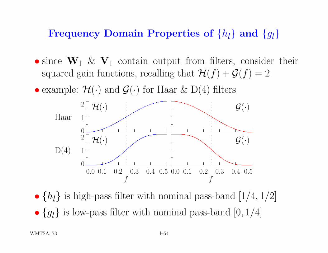
Frequency Domain Properties of {hl} and {gl}

• since W1 & V1 contain output from filters, consider theirsquared gain functions, recalling that H(f) + G(f) = 2

• example: H(·) and G(·) for Haar & D(4) filters

HaarH(·) G(·)

D(4)H(·) G(·)

2

1

02

1

00.0 0.1 0.2 0.3 0.4 0.5 0.0 0.1 0.2 0.3 0.4 0.5

f f

• {hl} is high-pass filter with nominal pass-band [1/4, 1/2]

• {gl} is low-pass filter with nominal pass-band [0, 1/4]

WMTSA: 73 I–54

Frequency Domain Properties of {hl} and {gl}

• since W1 & V1 contain output from filters, consider theirsquared gain functions, recalling that H(f) + G(f) = 2

• example: H(·) and G(·) for Haar & LA(8) filters

HaarH(·) G(·)

LA(8)H(·) G(·)

2

1

02

1

00.0 0.1 0.2 0.3 0.4 0.5 0.0 0.1 0.2 0.3 0.4 0.5

f f

• {hl} is high-pass filter with nominal pass-band [1/4, 1/2]

• {gl} is low-pass filter with nominal pass-band [0, 1/4]

WMTSA: 73 I–54

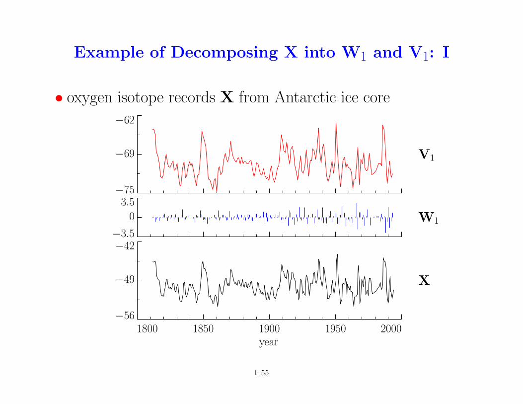
Example of Decomposing X into W1 and V1: I

• oxygen isotope records X from Antarctic ice core

V1

W1

X

−62

−69

−753.5

0

−3.5−42

−49

−561800 1850 1900 1950 2000

year

I–55

Example of Decomposing X into W1 and V1: II

• oxygen isotope record series X has N = 352 observations

• spacing between observations is ∆.= 0.5 years

• used Haar DWT, obtaining 176 scaling and wavelet coefficients

• scaling coefficients V1 related to averages on scale of 2∆

• wavelet coefficients W1 related to changes on scale of ∆

• coefficients V1,t and W1,t plotted against mid-point of yearsassociated with X2t and X2t+1

• note: variability in wavelet coefficients increasing with time(thought to be due to diffusion)

• data courtesy of Lars Karlof, Norwegian Polar Institute, PolarEnvironmental Centre, Tromsø, Norway

I–56

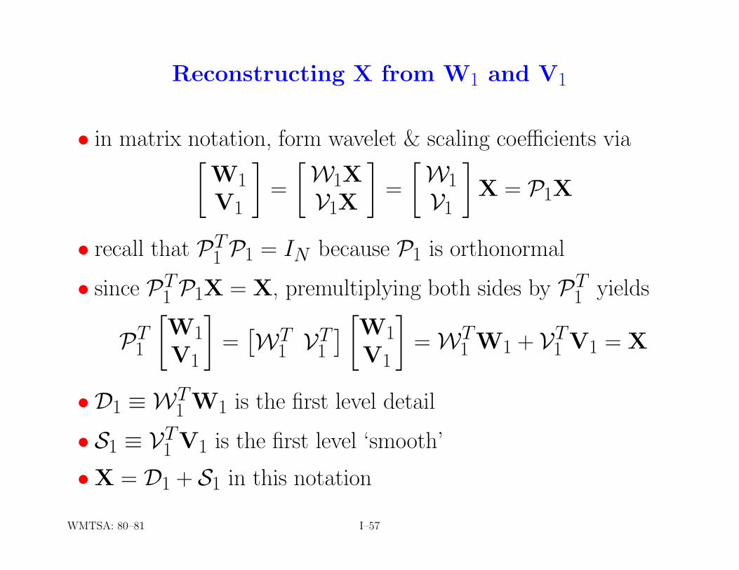
Reconstructing X from W1 and V1

• in matrix notation, form wavelet & scaling coefficients via∑W1V1

∏=

∑W1XV1X

∏=

∑W1V1

∏X = P1X

• recall that PT1 P1 = IN because P1 is orthonormal

• since PT1 P1X = X, premultiplying both sides by PT

1 yields

PT1

∑W1V1

∏=

£WT

1 VT1

§ ∑W1V1

∏= WT

1 W1 + VT1 V1 = X

• D1 ≡WT1 W1 is the first level detail

• S1 ≡ VT1 V1 is the first level ‘smooth’

•X = D1 + S1 in this notation

WMTSA: 80–81 I–57

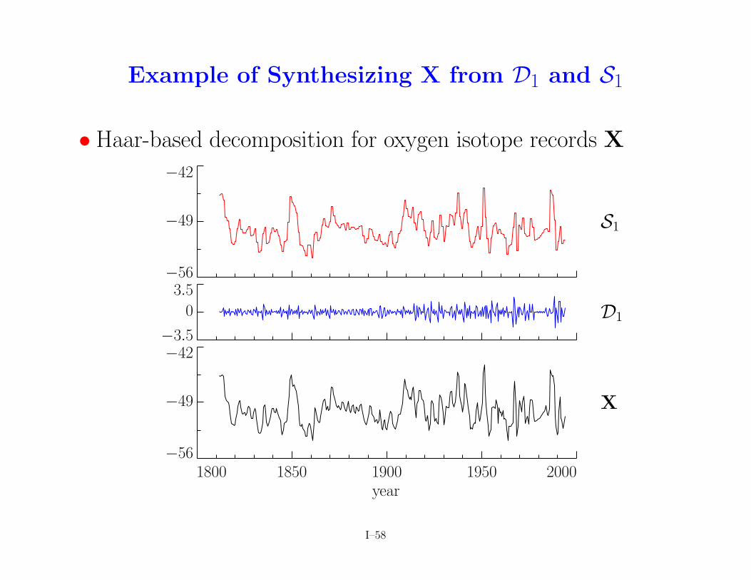
Example of Synthesizing X from D1 and S1

• Haar-based decomposition for oxygen isotope records X

S1

D1

X

−42

−49

−563.5

0

−3.5−42

−49

−561800 1850 1900 1950 2000

year

I–58

First Level Variance Decomposition: I

• recall that ‘energy’ in X is its squared norm kXk2

• because P1 is orthonormal, have PT1 P1 = IN and hence

kP1Xk2 = (P1X)TP1X = XTPT1 P1X = XTX = kXk2

• can conclude that kXk2 = kW1k2 + kV1k2 because

P1X =

∑W1V1

∏and hence kP1Xk2 = kW1k2 + kV1k2

• leads to a decomposition of the sample variance for X:

σ2X ≡ 1

N

N−1X

t=0

°Xt −X

¢2=

1

NkXk2 −X

2

=1

NkW1k2 +

1

NkV1k2 −X

2

I–59

First Level Variance Decomposition: II

• breaks up σ2X into two pieces:

1. 1NkW1k2, attributable to changes in averages over scale 1

2. 1NkV1k2 −X

2, attributable to averages over scale 2

• Haar-based example for oxygen isotope records

− first piece: 1NkW1k2 .

= 0.295

− second piece: 1NkV1k2 −X

2 .= 2.909

− sample variance: σ2X

.= 3.204

− changes on scale of ∆.= 0.5 years account for 9% of σ2

X(standardized scale 1 corresponds to physical scale ∆)

I–60

Summary of First Level of Basic Algorithm

• transforms {Xt : t = 0, . . . , N − 1} into 2 types of coefficients

•N/2 wavelet coefficients {W1,t} associated with:

−W1, a vector consisting of first N/2 elements of W

− changes on scale 1 and nominal frequencies 14 ≤ |f | ≤ 1

2− first level detail D1

−W1, an N2 ×N matrix consisting of first N

2 rows of W•N/2 scaling coefficients {V1,t} associated with:

−V1, a vector of length N/2

− averages on scale 2 and nominal frequencies 0 ≤ |f | ≤ 14

− first level smooth S1

− V1, an N2 × N matrix spanning same subspace as last N/2

rows of WWMTSA: 86–87 I–61

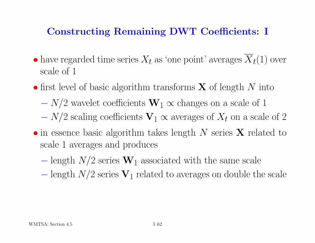
Constructing Remaining DWT Coefficients: I

• have regarded time series Xt as ‘one point’ averages Xt(1) overscale of 1

• first level of basic algorithm transforms X of length N into

−N/2 wavelet coefficients W1 ∝ changes on a scale of 1

−N/2 scaling coefficients V1 ∝ averages of Xt on a scale of 2

• in essence basic algorithm takes length N series X related toscale 1 averages and produces

− length N/2 series W1 associated with the same scale

− length N/2 series V1 related to averages on double the scale

WMTSA: Section 4.5 I–62

Constructing Remaining DWT Coefficients: II

• Q: what if we now treat V1 in the same manner as X?

• basic algorithm will transform length N/2 series V1 into

− length N/4 series W2 associated with the same scale (2)

− length N/4 series V2 related to averages on twice the scale

• by definition, W2 contains the level 2 wavelet coefficients

• Q: what if we treat V2 in the same way?

• basic algorithm will transform length N/4 series V2 into

− length N/8 series W3 associated with the same scale (4)

− length N/8 series V3 related to averages on twice the scale

• by definition, W3 contains the level 3 wavelet coefficients

WMTSA: Sections 4.5 and 4.6 I–63

Constructing Remaining DWT Coefficients: III

• continuing in this manner defines remaining subvectors of W(recall that W = WX is the vector of DWT coefficients)

• at each level j, outputs Wj and Vj from the basic algorithmare each half the length of the input Vj−1

• length of Vj given by N/2j

• since N = 2J , length of VJ is 1, at which point we must stop

• J applications of the basic algorithm defines the remainingsubvectors W2, . . ., WJ , VJ of DWT coefficient vector W

• overall scheme is known as the ‘pyramid’ algorithm

WMTSA: Section 4.6, 100–101 I–64

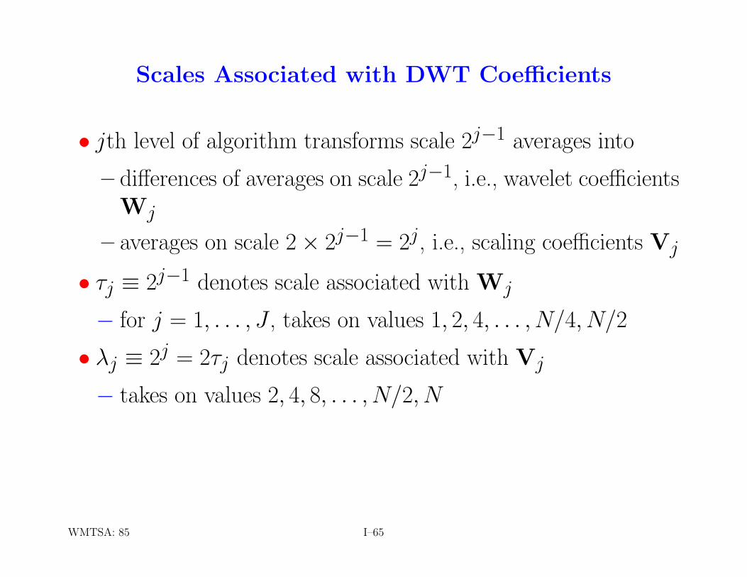
Scales Associated with DWT Coefficients

• jth level of algorithm transforms scale 2j−1 averages into

– differences of averages on scale 2j−1, i.e., wavelet coefficientsWj

– averages on scale 2× 2j−1 = 2j, i.e., scaling coefficients Vj

• τj ≡ 2j−1 denotes scale associated with Wj

− for j = 1, . . . , J , takes on values 1, 2, 4, . . . , N/4, N/2

• λj ≡ 2j = 2τj denotes scale associated with Vj

− takes on values 2, 4, 8, . . . , N/2, N

WMTSA: 85 I–65

Matrix Description of Pyramid Algorithm: I

• form N2j × N

2j−1 matrix Bj in same way as N2 ×N matrix W1

• when L = 4 and N/2j−1 = 16, have

Bj =

h1 h0 0 0 0 0 0 0 0 0 0 0 0 0 h3 h2h3 h2 h1 h0 0 0 0 0 0 0 0 0 0 0 0 00 0 h3 h2 h1 h0 0 0 0 0 0 0 0 0 0 00 0 0 0 h3 h2 h1 h0 0 0 0 0 0 0 0 00 0 0 0 0 0 h3 h2 h1 h0 0 0 0 0 0 00 0 0 0 0 0 0 0 h3 h2 h1 h0 0 0 0 00 0 0 0 0 0 0 0 0 0 h3 h2 h1 h0 0 00 0 0 0 0 0 0 0 0 0 0 0 h3 h2 h1 h0

• matrix gets us jth level wavelet coefficients via Wj = BjVj−1

WMTSA: 94 I–66

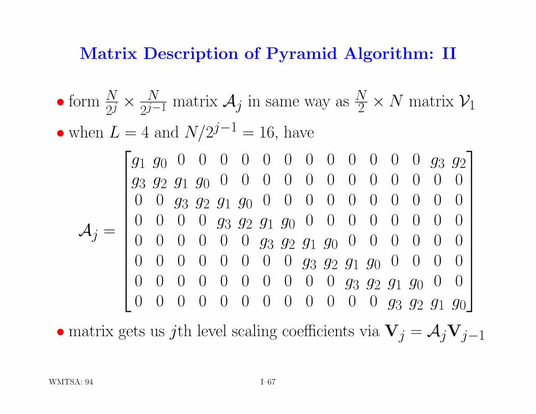
Matrix Description of Pyramid Algorithm: II

• form N2j × N

2j−1 matrix Aj in same way as N2 ×N matrix V1

• when L = 4 and N/2j−1 = 16, have

Aj =

g1 g0 0 0 0 0 0 0 0 0 0 0 0 0 g3 g2g3 g2 g1 g0 0 0 0 0 0 0 0 0 0 0 0 00 0 g3 g2 g1 g0 0 0 0 0 0 0 0 0 0 00 0 0 0 g3 g2 g1 g0 0 0 0 0 0 0 0 00 0 0 0 0 0 g3 g2 g1 g0 0 0 0 0 0 00 0 0 0 0 0 0 0 g3 g2 g1 g0 0 0 0 00 0 0 0 0 0 0 0 0 0 g3 g2 g1 g0 0 00 0 0 0 0 0 0 0 0 0 0 0 g3 g2 g1 g0

• matrix gets us jth level scaling coefficients via Vj = AjVj−1

WMTSA: 94 I–67

Matrix Description of Pyramid Algorithm: III

• if we define V0 = X and let j = 1, then

Wj = BjVj−1 reduces to W1 = B1V0 = B1X = W1X

because B1 has the same definition as W1

• likewise, when j = 1,

Vj = AjVj−1 reduces to V1 = A1V0 = A1X = V1X

because A1 has the same definition as V1

WMTSA: 94 I–68

Formation of Submatrices of W: I

• using Vj = AjVj−1 repeatedly and V1 = A1X, can write

Wj = BjVj−1

= BjAj−1Vj−2

= BjAj−1Aj−2Vj−3

= BjAj−1Aj−2 · · · A1X ≡WjX,

where Wj is N2j ×N submatrix of W responsible for Wj

• likewise, can get 1×N submatrix VJ responsible for VJ

VJ = AJVJ−1= AJAJ−1VJ−2= AJAJ−1AJ−2VJ−3= AJAJ−1AJ−2 · · · A1X ≡ VJX

• VJ is the last row of W , & all its elements are equal to 1/√

N

WMTSA: 94 I–69

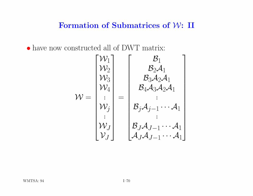
Formation of Submatrices of W: II

• have now constructed all of DWT matrix:

W =

W1W2W3W4...Wj...

WJVJ

=

B1B2A1B3A2A1B4A3A2A1

...BjAj−1 · · · A1

...BJAJ−1 · · · A1AJAJ−1 · · · A1

WMTSA: 94 I–70

Examples of W and its Partitioning: I

•N = 16 case for Haar DWT matrix W

................................................................................

................

................................

................

................

................

................

................

................

................................

W1

W2

W3

W4

V4

0

1

23

4

5

6

7

8

9

1011

12

13

14

15

0 5 10 15t

0 5 10 15t

• above agrees with qualitative description given previously

I–71

Examples of W and its Partitioning: II

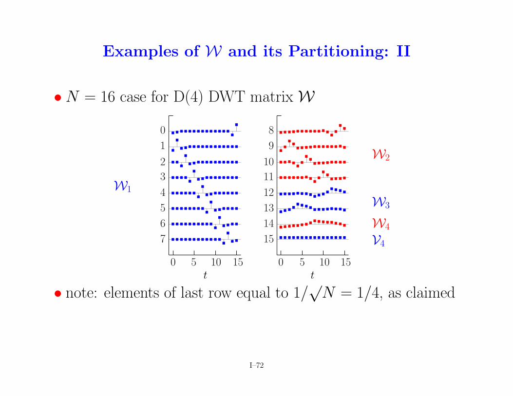
•N = 16 case for D(4) DWT matrix W

................................................................

................

................................................

................

................

................

................

................

................................................

W1

W2

W3

W4

V4

0

1

23

4

5

6

7

8

9

1011

12

13

14

15

0 5 10 15t

0 5 10 15t

• note: elements of last row equal to 1/√

N = 1/4, as claimed

I–72

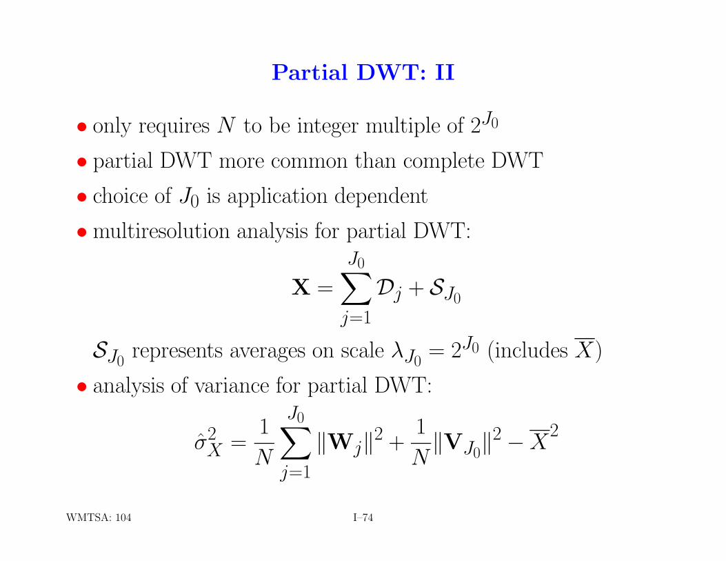
Partial DWT: I

• J repetitions of pyramid algorithm for X of length N = 2J

yields ‘complete’ DWT, i.e., W = WX

• can choose to stop at J0 < J repetitions, yielding a ‘partial’DWT of level J0:

W1W2...Wj...

WJ0VJ0

X =

B1B2A1

...BjAj−1 · · · A1

...BJ0

AJ0−1 · · · A1AJ0

AJ0−1 · · · A1

X =

W1W2

...Wj

...WJ0VJ0

• VJ0is N

2J0×N , yielding N

2J0coefficients for scale λJ0

= 2J0

WMTSA: 104 I–73

Partial DWT: II

• only requires N to be integer multiple of 2J0

• partial DWT more common than complete DWT

• choice of J0 is application dependent

• multiresolution analysis for partial DWT:

X =J0X

j=1

Dj + SJ0

SJ0represents averages on scale λJ0

= 2J0 (includes X)

• analysis of variance for partial DWT:

σ2X =

1

N

J0X

j=1

kWjk2 +1

NkVJ0

k2 −X2

WMTSA: 104 I–74

Example of J0 = 4 Partial Haar DWT


V4

W4

W3

W2

W1

X−44.2

−53.81800 1850 1900 1950 2000

year

I–75

Example of MRA from J0 = 4 Partial Haar DWT


S4

D4

D3

D2

D1

X

−44.2

−49.0

−53.81800 1850 1900 1950 2000

year

I–76

Example of Variance Decomposition

• decomposition of sample variance from J0 = 4 partial DWT

σ2X ≡ 1

N

N−1X

t=0

°Xt −X

¢2=

4X

j=1

1

NkWjk2 +

1

NkV4k2 −X

2

• Haar-based example for oxygen isotope records

− 0.5 year changes: 1NkW1k2 .

= 0.295 (.= 9.2% of σ2

X)

− 1.0 years changes: 1NkW2k2 .

= 0.464 (.= 14.5%)


= 0.652 (.= 20.4%)


= 0.846 (.= 26.4%)

− 8.0 years averages: 1NkV4k2 −X

2 .= 0.947 (

.= 29.5%)


.= 3.204

I–77

Haar Equivalent Wavelet & Scaling Filters

................................

....

........

................

{hl}

{h2,l}

{h3,l}

{h4,l}

{gl}

{g2,l}

{g3,l}

{g4,l}

L = 2

L2 = 4

L3 = 8

L4 = 16

L = 2

L2 = 4

L3 = 8

L4 = 16

• Lj = 2j is width of {hj,l} and {gj,l}• note: convenient to define {h1,l} to be same as {hl}

I–78

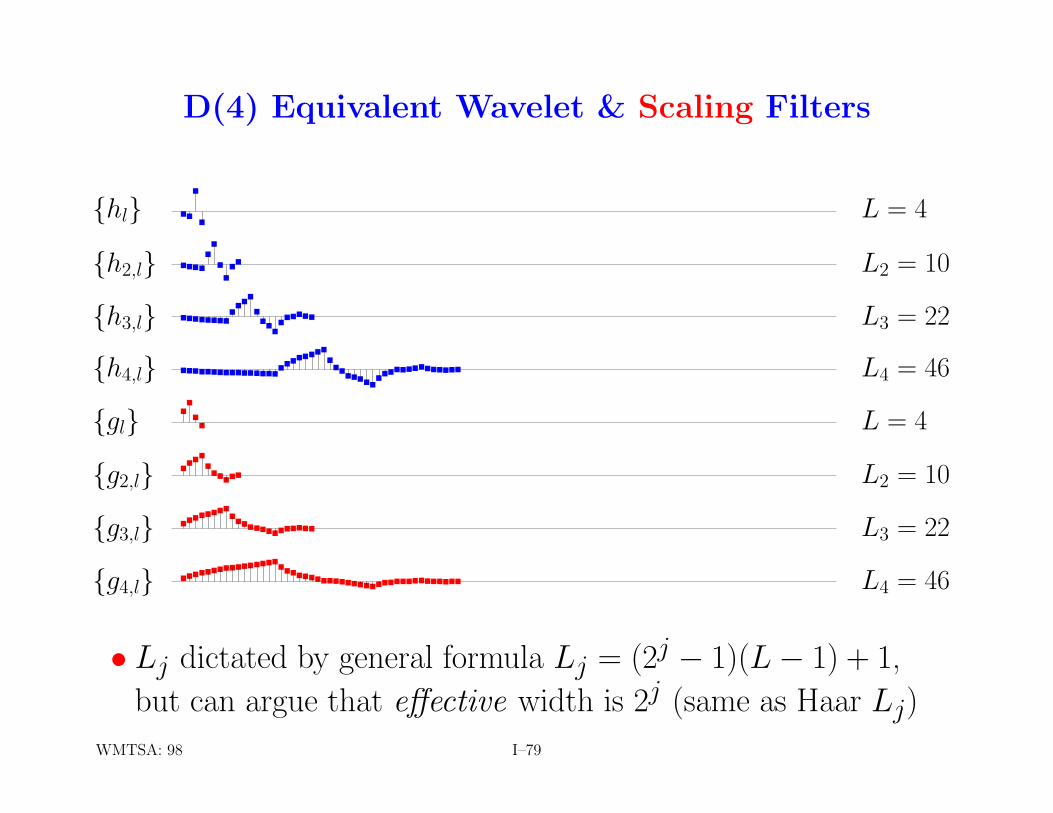
D(4) Equivalent Wavelet & Scaling Filters

....

..........

......................

..................................................

..........

......................

..............................................

{hl}

{h2,l}

{h3,l}

{h4,l}

{gl}

{g2,l}

{g3,l}

{g4,l}

L = 4

L2 = 10

L3 = 22

L4 = 46

L = 4

L2 = 10

L3 = 22

L4 = 46

• Lj dictated by general formula Lj = (2j − 1)(L− 1) + 1,but can argue that effective width is 2j (same as Haar Lj)

WMTSA: 98 I–79

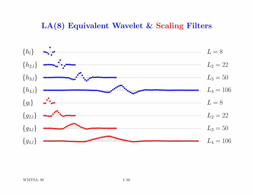
LA(8) Equivalent Wavelet & Scaling Filters

........

......................

..................................................

..........................................................................................................

........

......................

..................................................

..........................................................................................................

{hl}

{h2,l}

{h3,l}

{h4,l}

{gl}

{g2,l}

{g3,l}

{g4,l}

L = 8

L2 = 22

L3 = 50

L4 = 106

L = 8

L2 = 22

L3 = 50

L4 = 106

WMTSA: 98 I–80

Squared Gain Functions for Filters

• squared gain functions give us frequency domain properties:

Hj(f) ≡ |Hj(f)|2 and Gj(f) ≡ |Gj(f)|2

• example: squared gain functions for LA(8) J0 = 4 partial DWT

G4(·)

H4(·)

H3(·)

H2(·)

H1(·)

16

016

08

04

02

00 1

1618

316

14

516

38

716

12

f

WMTSA: 99 I–81

Maximal Overlap Discrete Wavelet Transform

• abbreviation is MODWT (pronounced ‘mod WT’)

• transforms very similar to the MODWT have been studied inthe literature under the following names:

− undecimated DWT (or nondecimated DWT)

− stationary DWT

− translation invariant DWT

− time invariant DWT

− redundant DWT

• also related to notions of ‘wavelet frames’ and ‘cycle spinning’

• basic idea: use values removed from DWT by downsampling

WMTSA: 159 I–82

Quick Comparison of the MODWT to the DWT

• unlike the DWT, MODWT is not orthonormal (in fact MODWTis highly redundant)

• unlike the DWT, MODWT is defined naturally for all samplessizes (i.e., N need not be a multiple of a power of two)

• similar to the DWT, can form multiresolution analyses (MRAs)using MODWT with certain additional desirable features; e.g.,unlike the DWT, MODWT-based MRA has details and smoothsthat shift along with X (if X has detail eDj, then T mX has

detail T m eDj, where T m circularly shifts X by m units)

• similar to the DWT, an analysis of variance (ANOVA) can bebased on MODWT wavelet coefficients

• unlike the DWT, MODWT discrete wavelet power spectrumsame for X and its circular shifts T mX

WMTSA: 159–160 I–83

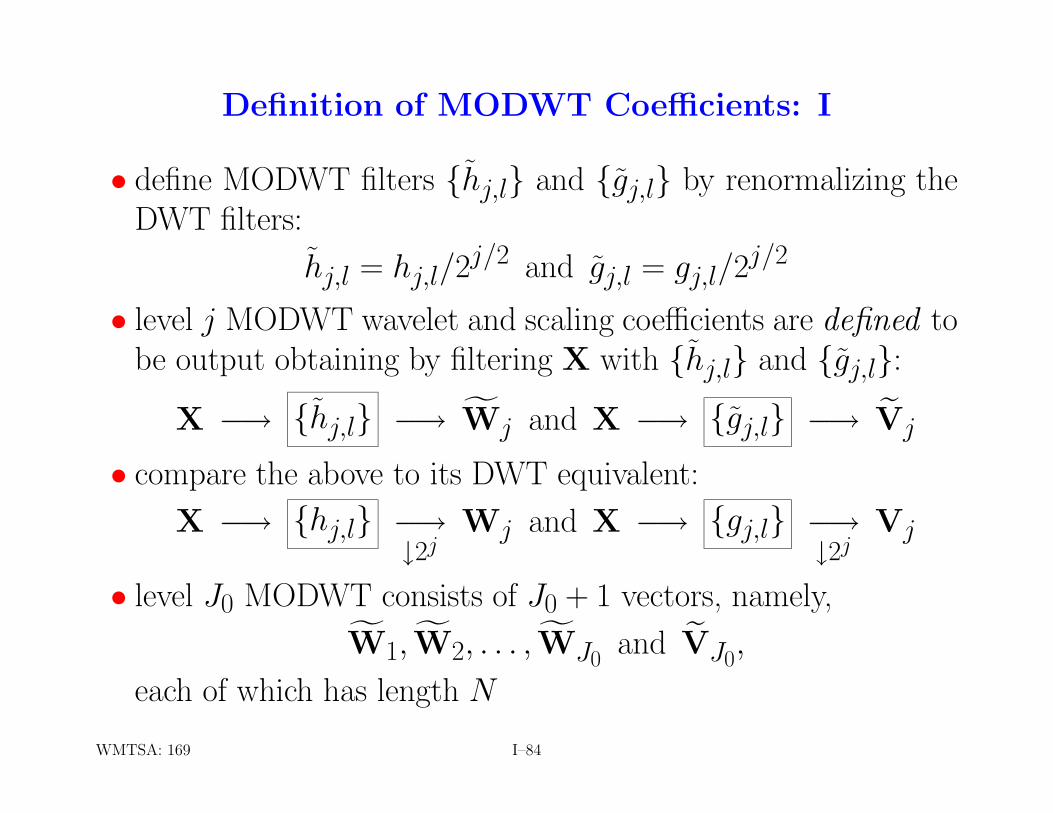
Definition of MODWT Coefficients: I

• define MODWT filters {hj,l} and {gj,l} by renormalizing theDWT filters:

hj,l = hj,l/2j/2 and gj,l = gj,l/2j/2

• level j MODWT wavelet and scaling coefficients are defined tobe output obtaining by filtering X with {hj,l} and {gj,l}:

X −→ {hj,l} −→ fWj and X −→ {gj,l} −→ eVj

• compare the above to its DWT equivalent:

X −→ {hj,l} −→↓2j

Wj and X −→ {gj,l} −→↓2j

Vj

• level J0 MODWT consists of J0 + 1 vectors, namely,fW1, fW2, . . . , fWJ0

and eVJ0,

each of which has length N

WMTSA: 169 I–84

Definition of MODWT Coefficients: II

• MODWT of level J0 has (J0 + 1)N coefficients, whereas DWThas N coefficients for any given J0

• whereas DWT of level J0 requires N to be integer multiple of2J0, MODWT of level J0 is well-defined for any sample size N

• when N is divisible by 2J0, we can write

Wj,t =

Lj−1X

l=0

hj,lX2j(t+1)−1−l mod N & fWj,t =

Lj−1X

l=0

hj,lXt−l mod N,

and we have the relationship

Wj,t = 2j/2fWj,2j(t+1)−1 &, likewise, VJ0,t = 2J0/2eVJ0,2J0(t+1)−1

(here fWj,t & eVJ0,t denote the tth elements of fWj & eVJ0)

WMTSA: 96–97, 169, 203 I–85

Properties of the MODWT

• as was true with the DWT, we can use the MODWT to obtain

− a scale-based additive decomposition (MRA):

X =J0X

j=1

eDj + eSJ0

− a scale-based energy decomposition (basis for ANOVA):

kXk2 =J0X

j=1

kfWjk2 + keVJ0k2

• in addition, the MODWT can be computed efficiently via apyramid algorithm

WMTSA: 159–160 I–86

Example of J0 = 4 LA(8) MODWT


T −45 eV4

T −53fW4

T −25fW3

T −11fW2

T −4fW1

X

−44.2

−53.81800 1850 1900 1950 2000

year

I–87

Relationship Between MODWT and DWT

• bottom plot shows W4 from DWT after circular shift T −3 toalign coefficients properly in time

• top plot shows fW4 from MODWT and subsamples that, uponrescaling, yield W4 via W4,t = 4fW4,16(t+1)−1

T −53fW4

T −3W4

3

0

−312

0

−121800 1850 1900 1950 2000

year

I–88

Example of J0 = 4 LA(8) MODWT MRA


eS4

eD4

eD3

eD2

eD1

X

−44.2

−53.81800 1850 1900 1950 2000

year

I–89

Example of Variance Decomposition

• decomposition of sample variance from MODWT

σ2X ≡ 1

N

N−1X

t=0

°Xt −X

¢2=

4X

j=1

1

NkfWjk2 +

1

NkeV4k2 −X

2

• LA(8)-based example for oxygen isotope records

− 0.5 year changes: 1NkfW1k2 .

= 0.145 (.= 4.5% of σ2

X)

− 1.0 years changes: 1NkfW2k2 .

= 0.500 (.= 15.6%)


= 0.751 (.= 23.4%)


= 0.839 (.= 26.2%)

− 8.0 years averages: 1NkeV4k2 −X

2 .= 0.969 (

.= 30.2%)


.= 3.204

I–90

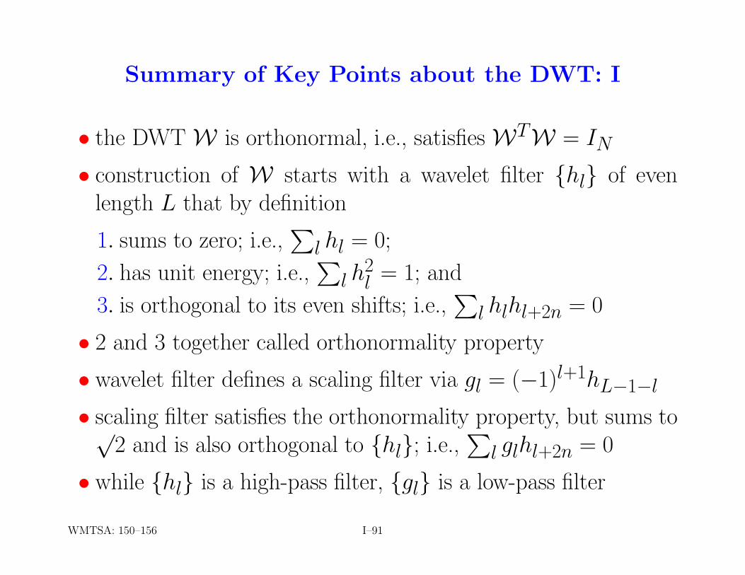
Summary of Key Points about the DWT: I

• the DWT W is orthonormal, i.e., satisfies WTW = IN

• construction of W starts with a wavelet filter {hl} of evenlength L that by definition

1. sums to zero; i.e.,P

l hl = 0;

2. has unit energy; i.e.,P

l h2l = 1; and

3. is orthogonal to its even shifts; i.e.,P

l hlhl+2n = 0

• 2 and 3 together called orthonormality property

• wavelet filter defines a scaling filter via gl = (−1)l+1hL−1−l

• scaling filter satisfies the orthonormality property, but sums to√2 and is also orthogonal to {hl}; i.e.,

Pl glhl+2n = 0

• while {hl} is a high-pass filter, {gl} is a low-pass filter

WMTSA: 150–156 I–91

Summary of Key Points about the DWT: II

• {hl} and {gl} work in tandem to split time series X into

− wavelet coefficients W1 (related to changes in averages on aunit scale) and

− scaling coefficients V1 (related to averages on a scale of 2)

• {hl} and {gl} are then applied to V1, yielding

− wavelet coefficients W2 (related to changes in averages on ascale of 2) and

− scaling coefficients V2 (related to averages on a scale of 4)

• continuing beyond these first 2 levels, scaling coefficients Vj−1at level j − 1 are transformed into wavelet and scaling coeffi-cients Wj and Vj of scales τj = 2j−1 and λj = 2j

WMTSA: 150–156 I–92

Summary of Key Points about the DWT: III

• after J0 repetitions, this ‘pyramid’ algorithm transforms timeseries X whose length N is an integer multiple of 2J0 into DWTcoefficients W1, W2, . . ., WJ0

and VJ0(sizes of vectors are

N2 , N

4 , . . ., N2J0

and N2J0

, for a total of N coefficients in all)

• DWT coefficients lead to two basic decompositions

• first decomposition is additive and is known as a multiresolutionanalysis (MRA), in which X is reexpressed as

X =J0X

j=1

Dj + SJ0,

where Dj is a time series reflecting variations in X on scale τj,while SJ0

is a series reflecting its λJ0averages

WMTSA: 150–156 I–93

Summary of Key Points about the DWT: IV

• second decomposition reexpresses the energy (squared norm)of X on a scale by scale basis, i.e.,

kXk2 =J0X

j=1

kWjk2 + kVJ0k2,

leading to an analysis of the sample variance of X:

σ2X =

1

N

N−1X

t=0

°Xt −X

¢2

=1

N

J0X

j=1

kWjk2 +1

NkVJ0

k2 −X2

WMTSA: 150–156 I–94

Summary of Key Points about the MODWT

• similar to the DWT, the MODWT offers

− a scale-based multiresolution analysis

− a scale-based analysis of the sample variance

− a pyramid algorithm for computing the transform efficiently

• unlike the DWT, the MODWT is

− defined for all sample sizes (no ‘power of 2’ restrictions)

− unaffected by circular shifts to X in that coefficients, detailsand smooths shift along with X

− highly redundant in that a level J0 transform consists of(J0 + 1)N values rather than just N

• MODWT can eliminate ‘alignment’ artifacts, but its redundan-cies are problematic for some uses

WMTSA: 159–160 I–95

wavelet methods for time series analysiswavelet methods for time series analysis part i:...

Documents