wavelet-based signal processing of electromagnetic pulse generated waveforms · structure of...

Calhoun: The NPS Institutional Archive

Theses and Dissertations Thesis Collection

2007-09

Wavelet-based signal processing of electromagnetic

pulse generated waveforms

Ardolino, Richard S.

Monterey California. Naval Postgraduate School

http://hdl.handle.net/10945/3342

NAVAL

POSTGRADUATE SCHOOL

MONTEREY, CALIFORNIA

THESIS

Approved for public release, distribution is unlimited

WAVELET-BASED SIGNAL PROCESSING OF ELECTROMAGNETIC PULSE GENERATED

WAVEFORMS

by

Richard S. Ardolino

September 2007

Thesis Advisor: Murali Tummala Second Reader: Roberto Cristi

THIS PAGE INTENTIONALLY LEFT BLANK

i

REPORT DOCUMENTATION PAGE Form Approved OMB No. 0704-0188 Public reporting burden for this collection of information is estimated to average 1 hour per response, including the time for reviewing instruction, searching existing data sources, gathering and maintaining the data needed, and completing and reviewing the collection of information. Send comments regarding this burden estimate or any other aspect of this collection of information, including suggestions for reducing this burden, to Washington headquarters Services, Directorate for Information Operations and Reports, 1215 Jefferson Davis Highway, Suite 1204, Arlington, VA 22202-4302, and to the Office of Management and Budget, Paperwork Reduction Project (0704-0188) Washington DC 20503. 1. AGENCY USE ONLY (Leave blank)

2. REPORT DATE September 2007

3. REPORT TYPE AND DATES COVERED Master’s Thesis

4. TITLE AND SUBTITLE: Wavelet-Based Signal Processing of Electromagnetic Pulse Generated Waveforms 6. AUTHOR(S) Richard S. Ardolino

5. FUNDING NUMBERS

7. PERFORMING ORGANIZATION NAME(S) AND ADDRESS(ES) Naval Postgraduate School Monterey, CA 93943-5000

8. PERFORMING ORGANIZATION REPORT NUMBER

9. SPONSORING /MONITORING AGENCY NAME(S) AND ADDRESS(ES) N/A

10. SPONSORING/MONITORING AGENCY REPORT NUMBER

11. SUPPLEMENTARY NOTES The views expressed in this thesis are those of the author and do not reflect the official policy or position of the Department of Defense or the U.S. Government. 12a. DISTRIBUTION / AVAILABILITY STATEMENT Approved for public release, distribution is unlimited

12b. DISTRIBUTION CODE

13. ABSTRACT (maximum 200 words) This thesis investigated and compared alternative signal processing techniques that used wavelet-based methods instead of traditional frequency domain methods for processing measured electromagnetic pulse (EMP) waveforms. The primary focus of the research was equalization and filtering techniques for processing EMP signals in additive white noise. Signal equalization was conducted at the sub-band level through the use of Infinite Impulse Response (IIR) filters and channel response characteristics. A brief investigation of signal de-noising through wavelet thresholding was also conducted. This thesis also addressed and provided viable methods for signal extraction and DC bias removal for a given measured EMP waveform. The mean squared error is used as the basis for the comparison of the effectiveness of the equalization algorithm. It was found that wavelet techniques provided results that were as well or better than traditional Fourier techniques. In systems with additive noise , wavelet-based techniques exceeded the performance of the Fourier-based methods and surpassed them when de-noising techniques were used.

15. NUMBER OF PAGES

103

14. SUBJECT TERMS Electromagnetic Pulse Waveforms, Wavelets, Aircraft Testing, Equalization, Wideband Signal Processing

16. PRICE CODE

17. SECURITY CLASSIFICATION OF REPORT

Unclassified

18. SECURITY CLASSIFICATION OF THIS PAGE

Unclassified

19. SECURITY CLASSIFICATION OF ABSTRACT

Unclassified

20. LIMITATION OF ABSTRACT

UU

NSN 7540-01-280-5500 Standard Form 298 (Rev. 2-89) Prescribed by ANSI Std. 239-18

ii


iii

Approved for public release, distribution is unlimited

WAVELET-BASED SIGNAL PROCESSING OF ELECTROMAGNETIC PULSE GENERATED WAVEFORMS

Richard S. Ardolino Lieutenant Commander, United States Navy B.S., United States Naval Academy, 1997

Submitted in partial fulfillment of the requirements for the degree of

MASTER OF SCIENCE IN ELECTRICAL ENGINEERING

from the

NAVAL POSTGRADUATE SCHOOL September 2007

Author: Richard S. Ardolino

Approved by: Murali Tummala

Thesis Advisor

Roberto Cristi Second Reader

Jeffrey B. Knorr Chairman, Department of Electrical and Computer Engineering

iv


v

ABSTRACT

This thesis investigated and compared alternative signal processing techniques

that used wavelet-based methods instead of traditional frequency domain methods for

processing measured electromagnetic pulse (EMP) waveforms. The primary focus of the

research was equalization and filtering techniques for processing EMP signals in additive

white noise. Signal equalization was conducted at the sub-band level through the use of

Infinite Impulse Response (IIR) filters and channel response characteristics. A brief

investigation of signal de-noising through wavelet thresholding was also conducted. This

thesis also addressed and provided viable methods for signal extraction and DC bias

removal for a given measured EMP waveform. The mean squared error is used as the

basis for the comparison of the effectiveness of the equalization algorithm. It was found

that wavelet techniques provided results that were as well or better than traditional

Fourier techniques. In systems with additive noise, wavelet-based techniques exceeded

the performance of the Fourier-based methods and surpassed them when de-noising

techniques were used.

vi


vii

TABLE OF CONTENTS

I. INTRODUCTION........................................................................................................1 A. THESIS OBJECTIVE.....................................................................................1 B. THESIS ORGANIZATION............................................................................2

II. SIGNAL PROCESSING: TECHNIQUES AND DOMAINS ..................................3 A. SIGNAL DOMAINS........................................................................................3

1. Fourier Transform...............................................................................3 2. Discrete Fourier Transform (DFT) ....................................................4 3. Continuous-Time Wavelet Transform (CWT)..................................6 4. Discrete Wavelet Transform (DWT)..................................................7 5. Types of Wavelets ..............................................................................11 6. De-Noising...........................................................................................13

B. EQUALIZATION..........................................................................................15

III. SIGNAL PROCESSING OF AIRCRAFT TEST WAVEFORMS .......................19 A. AIRCRAFT TEST .........................................................................................19 B. EMP SIGNAL COLLECTION MODEL ....................................................21 C. EQUALIZATION OF THE ACQUIRED WAVEFORM..........................21 D. MEASURED SIGNAL CHARACTERISTICS ..........................................23 E. MEASURED CHANNEL RESPONSE .......................................................24 F. SIGNAL PRE-PROCESSING......................................................................26

1. Signal Extraction................................................................................26 2. DC Bias Cancellation.........................................................................29 3. Linear Interpolation of the Channel Frequency Response ............30

IV. EQUALIZATION METHODS AND WAVELET SCHEMES.............................33 A. EQUALIZATION..........................................................................................33

1. Equalization using Wavelets .............................................................33 2. Equalization Techniques ...................................................................34

a. Method 1 - Time Domain Filtering of Sub-band Time Domain Signals with Inverse IIR Filter ................................35

b. Method 2 – Frequency Domain Filtering using Channel Frequency Response ...............................................................36

c. Method 3 - Time Domain Filtering of Wavelet Coefficients using Inverse IIR Filter .....................................36

d. Method 4 – NAWC-AD Method..............................................37 B. SUB-BAND FILTERING AND NOISE REMOVAL.................................38

1. System Model with Additive White Gaussian Noise.......................38

V. SIMULATION RESULTS ........................................................................................41 A. SIMULATION MODEL FOR ANALYSIS OF SYSTEM WITH NO

ADDITIVE NOISE ........................................................................................41 1. Equalization with No Signal Extraction ..........................................43 2. Equalization with Signal Extraction ................................................45

viii

B. SIMULATION MODEL FOR ANALYSIS OF SYSTEM WITH WHITE NOISE ..............................................................................................47 1. Equalization Results with Additive Noise with No Signal

Extraction ...........................................................................................48 a. Results without De-Noising ....................................................48 b. Results using De-noising ........................................................49 c. Comparison against Other Waveforms ..................................51

2. Equalization Results with Additive Noise with Signal Extraction ...........................................................................................52 a. Results without De-Noising ....................................................53 b. Results with De-Noising..........................................................54

VI. CONCLUSIONS ........................................................................................................57 A. SIGNIFICANT RESULTS............................................................................57 B. RECOMMENDATIONS FOR FURTHER RESEARCH .........................58

APPENDIX.............................................................................................................................61 A. MAIN PROGRAMS .....................................................................................61

1. Program Producing Tables for Chapter V......................................61 2. Program that Produces Figures for Chapter V ..............................64

B. FUNCTIONS USED IN ABOVE MAIN PROGRAMS .............................69 1. AVEPOWER......................................................................................69 2. CALPROG2........................................................................................71 3. WAVEDECOM..................................................................................73 4. BUILDIIR...........................................................................................76 5. FILTERNRECONSTRUCT .............................................................78 6. POLYWAVEFIL1 .............................................................................79

C. NOTES ON DE-NOISING AND EXTRACTION......................................80 1. De-Noising...........................................................................................80 2. Extraction ...........................................................................................81

LIST OF REFERENCES......................................................................................................83

INITIAL DISTRIBUTION LIST .........................................................................................85

ix

LIST OF FIGURES

Figure 1. FFT of Signal with additive noise. (a) Original Signal: 1,024-Point Frequency Chirp with Additive White Noise. (b) FFT (magnitude response) of the Chirp Signal. ............................................................................................5

Figure 2. Two-level Wavelet Decomposition using a Tree-Structured Filter Bank (After Ref. [4]). ..................................................................................................8

Figure 3. Wavelet Reconstruction (After Ref. [4]). ..........................................................9 Figure 4. Detail and Approximation Coefficients of a Sinusoidal Chirp in Additive

Noise Using and Haar-wavelet Transform: (a) Given Chirp Signal of 1,024 Points. (b) Detail Level 1 Coefficient, f1. (c) Detail Level 2 Coefficients, f2. (d) Detail level 3 Coefficients, f3. (e) Approximation Level 3 Coefficients e3. .....................................................................................................................10

Figure 5. Types of Wavelet Basis Functions: (a) Haar Wavelet, (b) Daubechie’s Order 3 Wavelet, (c) Meyer Wavelet, (d) Coiflet Wavelet..............................12

Figure 6. Normalized Signal Values versus Hard and Soft Thresholding with a Threshold Value of Approximately 0.5 (After Ref. [5]). (a) Original Signal Values, x[n] with no thresholding or T = 0. (b) Hard Thresholded Signal Value, xHT[n] for T = 0.5. (c) Soft Thresholded Signal Value, xST[n] for T = 0.5.....................................................................................................................14

Figure 7. Generic Equalization of a Signal, s(t), that passes through a Channel, is Digitized to record as a discrete-time signal x[n] and then Equalized, [ ]s n . ..15

Figure 8. A Generic Block Diagram of Equalization System with discrete time input signal s[n]. The Channel and Equalization Filter Blocks are represented by the impulse responses h[n] and g[n] respectively. ...........................................16

Figure 9. Illustration of Aircraft Testing Process............................................................20 Figure 10. Block Diagram of the Aircraft Test Model......................................................21 Figure 11. Equalization Model..........................................................................................22 Figure 12. Example Recorded Waveforms at Various Aircraft Test Points. (a)

Waveform 1. (b) Waveform 2. (c) Waveform 3. (d) Waveform 4. .................23 Figure 13. Channel Responses and the Sampling Rates of Channel. (a) Channel

Frequency Response of “8694.cal.” (b) Difference in Frequency Values of Successive Frequency Index Points in Channel File “8694.cal.” (c) Channel Frequency Response of “wbal.cal.” (d) Difference in Frequency Values of Successive Frequency Index Points in Channel File “wbal.cal.” ....................25

Figure 14. Example of Signal Extraction. (a) Original Waveform. (b) Time Average Energy of Waveform. (c) Range of Time Average Energy After Signal Points Below Threshold Have Been Removed. (d) Final Extracted Signal. ...28

Figure 15. Signal with Varying Levels of Energy Threshold Values. (a) Threshold = 0.1. (b)Threshold = 1. (c) Threshold = 20. (d) Threshold = 80. ......................29

Figure 16. Linear Interpolation of Channel Response. Frequencies fchannel and fchannel+1 Represent Successive Points in the Channel Spectrum. Frequency fdata Represents Location of the Frequency Bin of Data in the Frequency Domain.............................................................................................................31

x

Figure 17. System model using Wavelet Processing for Equalization..............................33 Figure 18. Structure of Wavelet Analysis and Synthesis with Equalization Filtering. .....34 Figure 19. Method 1: Processing of Signal Waveforms Using Wavelet-Based

Techniques. ......................................................................................................35 Figure 20. Method 2: Processing of Signal Waveforms Using Wavelet-Based

Techniques, and Fourier Transforms. ..............................................................36 Figure 21. Method 3: Processing of Signal Waveforms Using Wavelet-Based

Techniques and IIR Filtering. ..........................................................................37 Figure 22. Method 4: Processing of Signal Waveforms Using Fourier Based

Transforms as Performed by NAWC-AD........................................................37 Figure 23. De-noising Model for Processing EMP Waveforms. ......................................38 Figure 24. System Diagram with the Addition of White Noise, w[n]...............................39 Figure 25. Basic Model of System Experiment. ...............................................................42 Figure 26. Basic Model of System Implementing Signal Extraction Technique..............42 Figure 27. Basic Model of System Experiment with the Addition of White Noise..........47 Figure 28. Basic Model of System Experiment with Additive White Noise and

Implementing Signal Extraction Technique. ...................................................48 Figure 29. No Signal Extraction and De-noising. (a) Waveform 1 with Additive Noise

Using Methods Using Daubechie’s Order 3 Wavelet Level 3. (b) Normalized Results Using Daubechie’s Order 3 Wavelet Using Level 3. ......49

Figure 30. No Signal Extraction. (a) Waveform1 with Additive Noise with De-noising Using Daubechie’s Order 3 Wavelet Level 3. (b) Normalized Results with De-noising Using Daubechie’s Order 3 Wavelet Using Level 3. ....................50

Figure 31. Waveform 1 with No Signal Extraction. (a) Original Input Signal. (b) Signal with Noise (SNR of 15 dB). (c) Equalized Signal Using Method 2 without De-noising Using Daubechie’s Order 3 Wavelet. (d) Equalization Using Method 2 with De-noising Using Daubechie’s Order 3 Wavelet. ........51

Figure 32. Comparison between Each of the Waveforms with No Signal Extraction and Normalized MSE Values and Using Daubechie’s Order 3, and 3 Levels of Decomposition.............................................................................................52

Figure 33. Results with Signal Extraction and without De-noising. (a) Waveform1 with Additive Noise Using Daubechie’s Order 3 Wavelet, Level 3. (b) Normalized Results with No De-noising Using Daubechie’s Order 3 Wavelet, Level 3. .............................................................................................53

Figure 34. MSE as a function of SNR with Signal Extraction and De-noising: (a) Waveform1 with Additive Noise Using Daubechie’s Order 3 Wavelet, Level 3. (b) Normalized values Using Daubechie’s Order 3 Wavelet, Level 3........................................................................................................................54

Figure 35. Waveform 1 with Signal Extraction: (a) Original Input Signal. (b) Signal with Noise (SNR of 15 dB). (c) Equalized Signal Using Method 2 without De-noising Using Daubechie’s Order 3 Wavelet. (d) Equalization Using Method 2 with De-noising Using Daubechie’s Order 3 Wavelet. ...................55

xi

LIST OF TABLES

Table 1. Mean Squared Error in dB Using All Three Techniques for Various Wavelet Basis Functions and Multiple Level Decompositions and the Fourier method. Signal is Not Extracted from Data. .......................................44

Table 2. Mean Squared Error in dB Using All Three Techniques for Various Wavelet Basis Functions and Multiple Level Decompositions and the Fourier method using the model in Figure 26..................................................46

xii


xiii

ACKNOWLEDGEMENTS

I would like to thank Professor Tummala for his assistance and guidance with

respect to this thesis. I also would like to thank the Electrical Engineering Department

staff and support for the outstanding experience and quality of education that I was

provided.

xiv


xv

EXECUTIVE SUMMARY

This thesis investigated and compared alternative signal processing techniques

that used wavelet-based methods instead of traditional frequency domain methods for

processing measured electromagnetic pulse (EMP) waveforms. The work was based on

an existing procedure developed at the Naval Air Warfare Center, Aircraft Division

(NAWC-AD), Patuxent River, MD that processed signals using Fourier transforms and

manual preprocessing techniques. This process involved the capture, preprocessing and

equalization of EMP signals that penetrated the exterior aircraft shell.

The primary focus of the work reported in this thesis was equalization and

filtering techniques for processing EMP signals in additive white noise. The physical

model of the NAWC-AD test procedure consisted of receiver and digital recording

equipment which can distort the desired EMP waveform’s characteristics prior to digital

storage. In order to minimize the error between the actual and recorded signal, channel

equalization and noise filtration were required. This signal equalization was conducted at

the sub-band level through the use of infinite impulse response (IIR) filters and actual

channel response characteristics. Wavelet based decomposition and synthesis provided

the mechanism for this sub-band analysis to occur. Using the wavelet techniques, a brief

investigation of signal de-noising through wavelet thresholding was also conducted. This

effort led to the development of a number of different equalization techniques for

comparison against the NAWC-AD Fourier equalization technique.

This thesis also addressed and provided viable methods for signal extraction and

DC bias removal for a given measured EMP waveform. The NAWC-AD method

employed manual procedures to identify and extract the recorded waveform based on

operator visual inspection. The use of time averaged energy computation with an

appropriately selected threshold provided the basis for pre-processing steps with

consistent results. By automating these procedural steps, consistency in testing results

could improve the overall aircraft testing process. The mean squared error is used as the

basis for the comparison of the effectiveness of the equalization algorithms.

xvi

It was found that wavelet techniques provided results that were as good or better

than traditional Fourier techniques employed by NAWC-AD. In systems with additive

noise, wavelet-based techniques exceeded the performance of the Fourier-based methods

and surpassed them when de-noising techniques were used. Results suggest that the

current method employed by NAWCAD works well in a low noise (high SNR)

environment based on the channel (equipment) response provided. Significant

improvement in performance of the proposed wavelet methods with de-noising is

obtained at low SNRs, a desirable outcome especially when the aircraft testing is

conducted under noisy conditions.

1

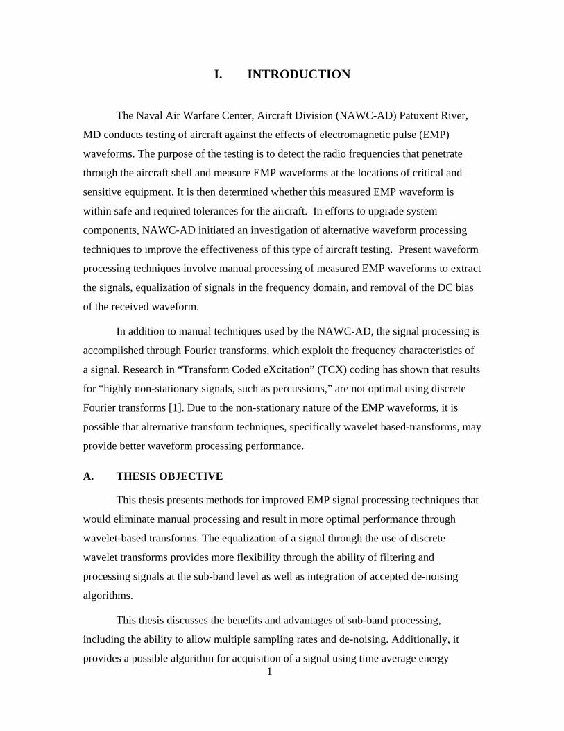
I. INTRODUCTION

The Naval Air Warfare Center, Aircraft Division (NAWC-AD) Patuxent River,

MD conducts testing of aircraft against the effects of electromagnetic pulse (EMP)

waveforms. The purpose of the testing is to detect the radio frequencies that penetrate

through the aircraft shell and measure EMP waveforms at the locations of critical and

sensitive equipment. It is then determined whether this measured EMP waveform is

within safe and required tolerances for the aircraft. In efforts to upgrade system

components, NAWC-AD initiated an investigation of alternative waveform processing

techniques to improve the effectiveness of this type of aircraft testing. Present waveform

processing techniques involve manual processing of measured EMP waveforms to extract

the signals, equalization of signals in the frequency domain, and removal of the DC bias

of the received waveform.

In addition to manual techniques used by the NAWC-AD, the signal processing is

accomplished through Fourier transforms, which exploit the frequency characteristics of

a signal. Research in “Transform Coded eXcitation” (TCX) coding has shown that results

for “highly non-stationary signals, such as percussions,” are not optimal using discrete

Fourier transforms [1]. Due to the non-stationary nature of the EMP waveforms, it is

possible that alternative transform techniques, specifically wavelet based-transforms, may

provide better waveform processing performance.

A. THESIS OBJECTIVE

This thesis presents methods for improved EMP signal processing techniques that

would eliminate manual processing and result in more optimal performance through

wavelet-based transforms. The equalization of a signal through the use of discrete

wavelet transforms provides more flexibility through the ability of filtering and

processing signals at the sub-band level as well as integration of accepted de-noising

algorithms.

This thesis discusses the benefits and advantages of sub-band processing,

including the ability to allow multiple sampling rates and de-noising. Additionally, it

provides a possible algorithm for acquisition of a signal using time average energy

2

computations. Performance of proposed techniques is evaluated through MATLAB

simulations using measured EMP waveforms with and without additive noise.

B. THESIS ORGANIZATION

Chapter II discusses the signal processing background required to address

manipulation and processing of measured EMP waveforms. Chapter III describes the

aircraft testing model and characteristics of the given measured EMP waveform data sets.

Chapter IV outlines the currently used procedures for signal processing in the system and

introduces proposed wavelet-based methods to process the EMP waveforms. Chapter V

presents the results of the proposed methods and their comparison to the Fourier method.

Chapter VI includes conclusions and topics for further research. Appendix A contains the

MATLAB code used to process the EMP waveforms.

3

II. SIGNAL PROCESSING: TECHNIQUES AND DOMAINS

This chapter provides the background for signal representations in the time

domain and frequency domain. It provides an overview of the Fourier transform

techniques that are the foundation of the currently used algorithms. It also introduces the

wavelet transforms and basic de-noising techniques. Finally, this chapter discusses the

basic concepts of channel filtering and equalization.

A. SIGNAL DOMAINS

A given signal, in particular an electro-magnetic waveform, can be analyzed by

using a number of different methods. The use of mathematical transformations can lead

to more versatile representation of signals for processing. For example, although some

characteristics of signals may not be evident in the time domain, definitive signal

properties may be clearly observed in the frequency domain. Fourier transform and

wavelet decomposition are two methods of expressing time domain signals in another

domain in order to extract information as well as perform processing with greater ease in

a computationally efficient manner.

1. Fourier Transform

Using the Fourier transform, it is possible to represent a given time-domain signal

as a function of all frequencies present in it. This is accomplished by representing a

signal ( )x t as a linear combination of complex exponentials [2], given by

( ) ( ) j tX x t e dtωω+∞

−

−∞

= ∫ (2.1)

where X(ω) is the transformed signal and ω is the radian frequency.

An inverse transform can be applied to transform a frequency domain signal X(ω)

to a time-domain signal x(t), given by

1( ) ( )2

j tx t X e dωω ωπ

+∞

−∞

= ∫ . (2.2)

4

The continuous-time Fourier transform, however, can only be applied to signals

of infinite duration and continuous time. Due to the wide-spread use of digital

technologies in modern signal processing applications, signals are commonly acquired

and stored digitally as a set of data points or a vector. For this reason, it is necessary to

utilize the discrete Fourier transform.

2. Discrete Fourier Transform (DFT)

The DFT is an extension of the Fourier transform to process digitized signal

sequences of finite duration and provides a one-to-one correspondence of a time domain

signal to its frequency domain counterpart for a given sampling rate. The transform also

represents the time-domain signal as a linear combination of complex exponentials, but

these exponentials occur at discrete frequency locations as opposed to over the

continuous spectrum.

In discrete signal processing, input signals are typically assembled as data vectors

of length N. If Ts is the sampling period of the digitized signals, the duration of a vector

containing N samples is N.Ts. The DFT of N samples of a discrete-time signal, x[n], is

given by [2]

[ ] [ ] ( )1

2

0

1 , 0,1, , 1N

jk N n

nX k x n e k N

Nπ

−−

=

= = −∑ … (2.3)

where n and k represent the time and frequency indices. The DFT represents the signal in

the frequency domain as a function of the digital frequency, 2d

kNπω = ; 0 2dω π≤ ≤ . The

digital frequency can be expressed as 2d

s

fFπω = where f is the analog frequency and

1s

s

FT

= is the sampling frequency. The width of each DFT frequency bin is sFfN

∆ = .

The fast Fourier transform (FFT) is a computationally efficient algorithm to

implement the DFT. The FFT utilizes a “divide and conquer” technique to perform the

DFT calculations quickly [3] by breaking a signal sequence down systematically into

smaller sequences. For the FFT to be effective, the sequence length must be an integer

5

power of 2. This can quickly be achieved by appending zeros to the end of a signal vector

called “zero padding,” which has no effect on the characteristics of the signal being

analyzed.

Figure 1 shows a chirp signal in the time-domain and its frequency-domain

representation (magnitude only) obtained by using a 1,024-point FFT algorithm. From

Figure 1, it can be seen that the signal contains stronger low frequency components than

high frequency components. However, where in time these components occur cannot be

determined from the frequency response. Other techniques, such as wavelet transforms,

not only provide frequency information of a signal, but also provide corresponding time

information as well when transformed. For this reason, the wavelet transforms are

described in the following sections.

0 100 200 300 400 500 600 700 800 900 1000-10

-5

0

5

10

-500 -400 -300 -200 -100 0 100 200 300 400 5000

100

200

300

400

500

Frequency Index(b)

Time Index(a)

Mag

nitu

deA

mpl

itude

0 100 200 300 400 500 600 700 800 900 1000-10

-5

0

5

10

-500 -400 -300 -200 -100 0 100 200 300 400 5000

100

200

300

400

500

Frequency Index(b)

Time Index(a)

Mag

nitu

deA

mpl

itude

Figure 1. FFT of Signal with additive noise. (a) Original Signal: 1,024-Point Frequency

Chirp with Additive White Noise. (b) FFT (magnitude response) of the Chirp Signal.

6

3. Continuous-Time Wavelet Transform (CWT)

The wavelet transform is another method for representing signals. The wavelet

transform has the ability to represent the time-frequency variations of signal components

in multiple discrete frequency bands, which can improve analysis of a given signal. The

CWT of a signal x(t) is defined as [4]

( ) ( ) 1, t uW u s x t dtss

ψ+∞

∗

−∞

−⎛ ⎞= ⎜ ⎟⎝ ⎠∫ (2.4)

where ψ(t) is the wavelet basis function; the variable u represents the time shifting of the

basis function and the variable s represents the scaling value of the wavelet basis

function. The wavelets basis, ψ(t), has a time average of zero:

( ) 0t dtψ+∞

−∞

=∫ (2.5)

For each basis function, a scaling function, ( )tφ , exists such that

2 2

1

( ) ( ) dst sts

φ ψ+∞

= ∫ (2.6)

and s represents the scaling value of the function for radian frequency ω as defined

above. The function, ψ(t) and ( )tφ , are orthogonal such that

*( ) ( ) 0t t dtψ φ+∞

−∞

=∫ (2.7)

ensuring that their projections into the wavelet domain are unique and consistent

transformation of the signal without loss or redundancy of information [4].

This transformation is more versatile than the Fourier transform. By manipulating

the shifting and scaling parameters, a signal transformed by wavelets provides a multi-

band representation that can detect and characterize transient components with a zooming

procedure across scales [4]. Wavelet types and their advantages are discussed further in

Chapter IV.

7

As with the Fourier transform, the discrete representation of a signal utilizing the

wavelet transform can also be found using the discrete wavelet transform. Additionally,

there is further discussion on the benefits of using wavelet transforms over Fourier

transforms in the following sections.

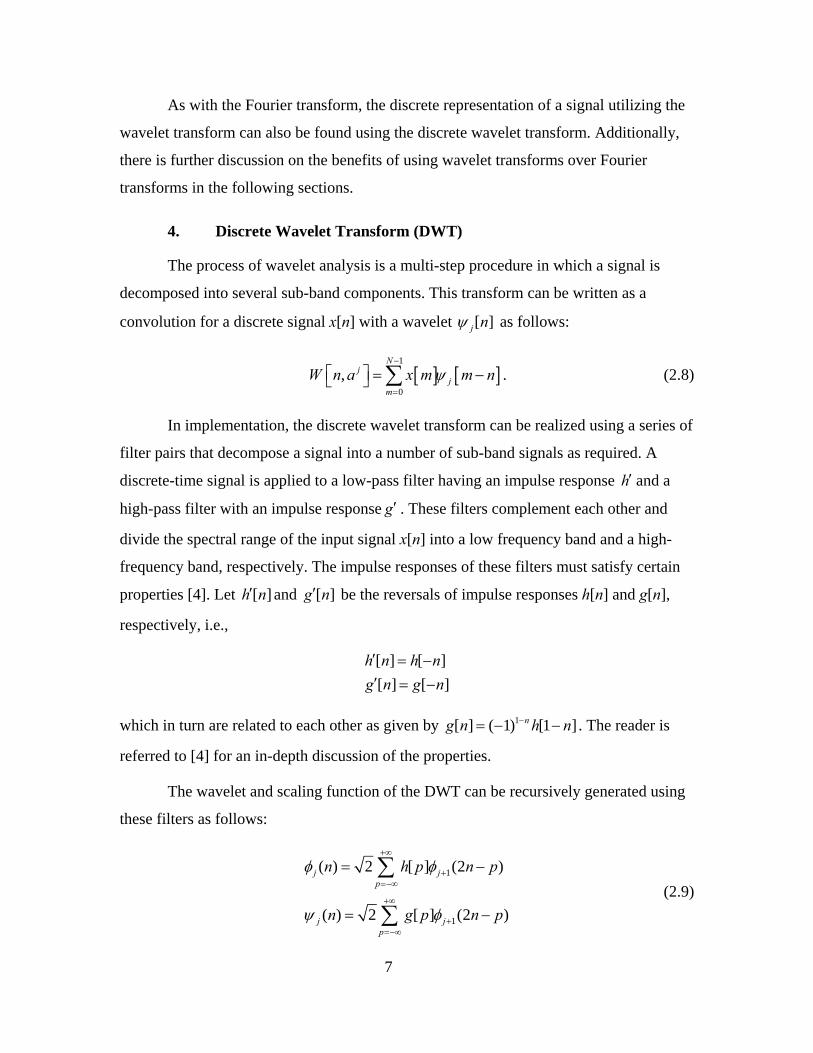
4. Discrete Wavelet Transform (DWT)

The process of wavelet analysis is a multi-step procedure in which a signal is

decomposed into several sub-band components. This transform can be written as a

convolution for a discrete signal x[n] with a wavelet [ ]j nψ as follows:

[ ] [ ]1

0,

Nj

jm

W n a x m m nψ−

=

⎡ ⎤ = −⎣ ⎦ ∑ . (2.8)

In implementation, the discrete wavelet transform can be realized using a series of

filter pairs that decompose a signal into a number of sub-band signals as required. A

discrete-time signal is applied to a low-pass filter having an impulse response h′ and a

high-pass filter with an impulse response g′ . These filters complement each other and

divide the spectral range of the input signal x[n] into a low frequency band and a high-

frequency band, respectively. The impulse responses of these filters must satisfy certain

properties [4]. Let [ ]h n′ and [ ]g n′ be the reversals of impulse responses h[n] and g[n],

respectively, i.e.,

[ ] [ ][ ] [ ]

h n h ng n g n′ = −′ = −

which in turn are related to each other as given by 1[ ] ( 1) [1 ]ng n h n−= − − . The reader is

referred to [4] for an in-depth discussion of the properties.

The wavelet and scaling function of the DWT can be recursively generated using

these filters as follows:

1

1

( ) 2 [ ] (2 )

( ) 2 [ ] (2 )

j jp

j jp

n h p n p

n g p n p

φ φ

ψ φ

+∞

+=−∞

+∞

+=−∞

= −

= −

∑

∑ (2.9)

8

where n represents the time indices of the wavelet function, j represents the resolution

level, and the term 2 in (2 )n pφ − indicates a decimation operation by 2.

Let ej[n] and fj[n] represent the approximation and detail coefficients,

respectively, which are obtained as the following inner products [4]

[ ] [ ], [ ]

[ ] [ ], [ ]

j j

j j

e n x n n

f n x n n

φ

ψ

=

= (2.10)

These inner products in turn yield recursive operations for computing the approximation

and detail coefficients [4]:

1

1

[ ] [ 2 ] [ ]

[ ] [ 2 ] [ ]

j jp

j jp

e n h p n e p

f n g p n e p

+∞

−=−∞

+∞

−=−∞

= −

= −

∑

∑ (2.11)

where j defines the level of decomposition. Figure 2 shows a schematic of the

implementation of Equation (2.11). The decimation is represented by 2↓ in the figure.

Each level of decomposition results in approximation and detail coefficients denoted ej

and fj, respectively. Through repetitive iterations, this process can continue starting from

the original signal, e0, down to where fn and en are a length of one.

ej+2[n]

fj+2[n]

2

2

2

2

h'

g'

h'

g'

ej[n]

ej+1[n]

fj+1[n]

ej+2[n]

fj+2[n]

22

2

2

2

h'

g'

h'

g'

ej[n]

ej+1[n]

fj+1[n]

Figure 2. Two-level Wavelet Decomposition using a Tree-Structured Filter Bank (After

Ref. [4]).

9

Conversely, wavelet reconstruction is the process of taking sub-band coefficients

and rebuilding the signal to its original form. The signal reconstruction is given by [4]

1 1[ ] [ 2 ] [ ] [ 2 ] [ ]j j jp p

e n h n p e p g n p f p+∞ +∞

+ +=−∞ =−∞

= − + −∑ ∑ . (2.12)

As with wavelet decomposition, reconstruction employs a similar tree-like filter

bank structure as shown in Figure 3. In this diagram, the filters used are h and g, the

reversals of h' and g', respectively. The coefficients are filtered and then up-sampled by

two, denoted by the symbol 2↑ .

2

e'j+2[n]

f'j+2[n]e'j[n]

e'j+1[n]

f'j+1[n]

g

h

g

h

2

2

2

⊕

⊕

2

e'j+2[n]

f'j+2[n]e'j[n]

e'j+1[n]

f'j+1[n]

g

h

g

h

2

2

22

⊕

⊕

Figure 3. Wavelet Reconstruction (After Ref. [4]).

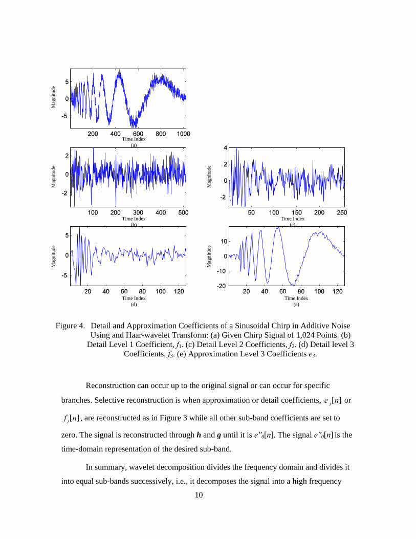
By using different wavelet basis functions or the number of levels, there are

multiple possible representations of time-domain signal. Figure 4 illustrates the results of

wavelet decomposition of an arbitrary 1,024-point frequency chirp signal with additive

noise and three levels of decomposition using the Haar-wavelet. As can be seen, the e3

coefficients shown in Figure 4 (e) contain the low frequency portion of the signal and are

of length 128 points. The f1 coefficients shown in Figure 4 (b) are the high frequency

coefficients of length 512.

10

Time Index(a)

Time Index(b)

Time Index(c)

Time Index(d)

Time Index(e)

Mag

nitu

deM

agni

tude

Mag

nitu

de

Mag

nitu

deM

agni

tude

Time Index(a)

Time Index(b)

Time Index(c)

Time Index(d)

Time Index(e)

Mag

nitu

deM

agni

tude

Mag

nitu

de

Mag

nitu

deM

agni

tude

Figure 4. Detail and Approximation Coefficients of a Sinusoidal Chirp in Additive Noise

Using and Haar-wavelet Transform: (a) Given Chirp Signal of 1,024 Points. (b) Detail Level 1 Coefficient, f1. (c) Detail Level 2 Coefficients, f2. (d) Detail level 3

Coefficients, f3. (e) Approximation Level 3 Coefficients e3.

Reconstruction can occur up to the original signal or can occur for specific

branches. Selective reconstruction is when approximation or detail coefficients, [ ]je n or

[ ]jf n , are reconstructed as in Figure 3 while all other sub-band coefficients are set to

zero. The signal is reconstructed through h and g until it is e''0[n]. The signal e''0[n] is the

time-domain representation of the desired sub-band.

In summary, wavelet decomposition divides the frequency domain and divides it

into equal sub-bands successively, i.e., it decomposes the signal into a high frequency

11

component and a low frequency component. As evident in Figure 4, each time the signal

decomposes to the next level, there are half as many points to represent the data than at

the level before. The wavelet decomposition in Figure 4 gives an alternative

representation of the sinusoidal chirp in additive noise compared to that given by the FFT

in Figure 1 (b). The fact that a different representation of the same signal exists leads to

the possibility of exploiting these representations using techniques not available to the

FFT-based signal processing.

5. Types of Wavelets

Wavelets have greater versatility than Fourier transforms because they allow for

multiple types of basis functions and multiple levels of decomposition. As discussed,

wavelet basis functions are associated in pairs as defined in Equations (2.4) and (2.5),

ψ(t), and a scaling function φ (t), and satisfy the relationship in Equation (2.6). As long

as the wavelet has a time average of zero as defined in Equation (2.5) and the scaling

function is orthogonal to the basis wavelet and satisfies Equation (2.8) and (2.9), it

constitutes a valid wavelet pair [5]. This allows virtually no limit on the number of

wavelet bases available. However, in the literature, some popular wavelet families have

emerged due to their superior performance.

For a given signal, some wavelets produce better results than other wavelets. For

example, the “Haar” wavelet is a square wave function, as depicted in Figure 5 (a) and

defined as

1 0 0.5

( )1 0.5 1

tt

tψ

≤ ≤⎧= ⎨− ≤ ≤⎩

(2.13)

with the ability to represent a square wave easily and accurately using only a few signal

samples. The corresponding Haar scaling function is given by

1 0 1( )

0t

totherwise

φ≤ ≤⎧

= ⎨⎩

However, for a typical sinusoidal signal, the “Haar” may not be the best basis function to

utilize.

12

Wavelets are generally classified into families. Some typical families are Haar,

Daubechie’s, Coiflet, and Meyer. With exception of the Haar and Meyer wavelets of this

sub set, the other wavelets do not have explicit expressions that define them. Figure 5

shows a plot of each respective wavelet type. Unless sufficient a priori information is

available for the signal and its correlation to a wavelet, it cannot be determined which

wavelet basis function will have the best results. Typically, wavelets are optimized when

there is a minimum number of wavelet coefficients that have values that are much greater

than zero [4, 5].

Time index(a)

Time index(b)

Time index(c)

Time index(d)

Mag

nitu

deM

agni

tude

Mag

nitu

deM

agni

tude

Time index(a)

Time index(b)

Time index(c)

Time index(d)

Mag

nitu

deM

agni

tude

Mag

nitu

deM

agni

tude

Figure 5. Types of Wavelet Basis Functions: (a) Haar Wavelet, (b) Daubechie’s Order 3

Wavelet, (c) Meyer Wavelet, (d) Coiflet Wavelet.

13

In this work, a subset of the different types of wavelet basis function are used and

compared. Those used in this work include Haar, Daubechie’s order 3 and 15, Coiflet,

and Meyer. No research was conducted to determine the best wavelet for this application.

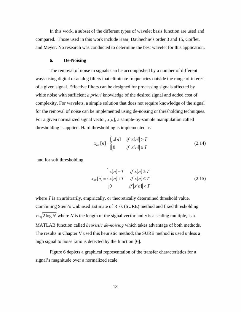
6. De-Noising

The removal of noise in signals can be accomplished by a number of different

ways using digital or analog filters that eliminate frequencies outside the range of interest

of a given signal. Effective filters can be designed for processing signals affected by

white noise with sufficient a priori knowledge of the desired signal and added cost of

complexity. For wavelets, a simple solution that does not require knowledge of the signal

for the removal of noise can be implemented using de-noising or thresholding techniques.

For a given normalized signal vector, x[n], a sample-by-sample manipulation called

thresholding is applied. Hard thresholding is implemented as

[ ] [ ]

[ ]0 [ ]HT

x n if x n Tx n

if x n T

⎧ >⎪= ⎨≤⎪⎩

(2.14)

and for soft thresholding

[ ] [ ]

[ ] [ ] [ ]0 [ ]

ST

x n T if x n Tx n x n T if x n T

if x n T

⎧ − ≥⎪

= + ≤⎨⎪ <⎩

(2.15)

where T is an arbitrarily, empirically, or theoretically determined threshold value.

Combining Stein’s Unbiased Estimate of Risk (SURE) method and fixed thresholding

2 log Nσ where N is the length of the signal vector and σ is a scaling multiple, is a

MATLAB function called heuristic de-noising which takes advantage of both methods.

The results in Chapter V used this heuristic method; the SURE method is used unless a

high signal to noise ratio is detected by the function [6].

Figure 6 depicts a graphical representation of the transfer characteristics for a

signal’s magnitude over a normalized scale.

14

0.5

0

-0.5

1

-10-1 1

Original Signal Hard thresholded Signal Soft thresholded Signal

0.5

0

-0.5

-10-1 1

0.5

0

-0.5

-10-1 1

Normalized Signal x[n]Magnitude Value

(a)

Normalized Signal x[n] Magnitude Value

(c)


(b)

Nor

mal

ized

Thr

esho

ld v

alue

Nor

mal

ized

Thr

esho

ld v

alue

, xH

T[n]

Nor

mal

ized

Thr

esho

ld v

alue

, xST

[n]

1 1T=0 T=0.5 T=0.5

0.5

0

-0.5

1

-10-1 1


0.5

0

-0.5

-10-1 1

0.5

0

-0.5

-10-1 1


(a)


(c)


(b)

Nor

mal

ized

Thr

esho

ld v

alue

Nor

mal

ized

Thr

esho

ld v

alue

, xH

T[n]

Nor

mal

ized

Thr

esho

ld v

alue

, xST

[n]

1 1

0.5

0

-0.5

1

-10-1 1


0.5

0

-0.5

-10-1 1

0.5

0

-0.5

-10-1 1


(a)


(c)


(b)

Nor

mal

ized

Thr

esho

ld v

alue

Nor

mal

ized

Thr

esho

ld v

alue

, xH

T[n]

Nor

mal

ized

Thr

esho

ld v

alue

, xST

[n]

1 1T=0 T=0.5 T=0.5

Figure 6. Normalized Signal Values versus Hard and Soft Thresholding with a Threshold

Value of Approximately 0.5 (After Ref. [5]). (a) Original Signal Values, x[n] with no thresholding or T = 0. (b) Hard Thresholded Signal Value, xHT[n] for T =

0.5. (c) Soft Thresholded Signal Value, xST[n] for T = 0.5.

To implement de-noising, a signal is decomposed into approximation and detail

coefficients using the wavelet transform. These resultant coefficients are then normalized

and a threshold value is calculated using the SURE method or 2 log N to minimize the

estimation error between the actual noise signal and the signal estimate without noise [4].

Wavelet coefficients are then compared against this threshold and the applicable

threshold is applied. All values above the threshold are left alone in the case of hard

thresholding shown in Figure 6 (b); in the case of soft thresholding, the values are scaled

lower as shown in Figure 6 (c). The assumption behind this method of processing is that

unless the magnitude of the coefficient exceeds a threshold value, it is a contribution

from noise and should be removed.

15

B. EQUALIZATION

A channel accounts for the effects of a transmission medium as a signal travels

from a source to a destination. In the channel, a signal can be amplified, attenuated,

dispersed in time, and distorted as a function of the characteristics of the physical

medium, which may be wireless or wired along with miscellaneous equipment. As a

result, every channel has a frequency response characteristic that will affect the signal as

it passes and will distort the signal from its original form. The purpose of equalization is

to nullify the effects of the channel characteristics and preserve the signal as close as

possible to its original form.

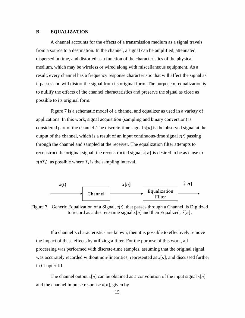
Figure 7 is a schematic model of a channel and equalizer as used in a variety of

applications. In this work, signal acquisition (sampling and binary conversion) is

considered part of the channel. The discrete-time signal x[n] is the observed signal at the

output of the channel, which is a result of an input continuous-time signal s(t) passing

through the channel and sampled at the receiver. The equalization filter attempts to

reconstruct the original signal; the reconstructed signal [ ]s n is desired to be as close to

s(nTs) as possible where Ts is the sampling interval.

Channel EqualizationFilter

s(t) x[n] ˆ[ ]s n

Channel EqualizationFilter

s(t) x[n] ˆ[ ]s n

Figure 7. Generic Equalization of a Signal, s(t), that passes through a Channel, is Digitized

to record as a discrete-time signal x[n] and then Equalized, [ ]s n .

If a channel’s characteristics are known, then it is possible to effectively remove

the impact of these effects by utilizing a filter. For the purpose of this work, all

processing was performed with discrete-time samples, assuming that the original signal

was accurately recorded without non-linearities, represented as s[n], and discussed further

in Chapter III.

The channel output x[n] can be obtained as a convolution of the input signal s[n]

and the channel impulse response h[n], given by

16

0

[ ] [ ] [ ] 0,1,.... 1L

kx n h k s n k n N

=

= − = −∑ (2.16)

where L is the length of the filter representing the channel. The linear operation of

convolution can be accomplished in the frequency domain as a product:

( ) ( ) ( )X S Hω ω ω= (2.17)

where X(ω) is the Discrete Time Fourier transform of the received signal x[n] and H(ω) is

the channel frequency response. Frequency domain implementation of convolution using

the FFT is computationally efficient and is the preferred method for signal analysis in

many applications.

The system model for equalization of a signal traversing through two filters

representing the channel and the equalization filter is shown in Figure 8. The input signal

to the channel is a discrete–time signal s[n]. In this model, the channel is assumed to

account for any imperfections in the data acquisition system. Ideally, the equalization

filter will have a frequency response that is the inverse of the channel. In other words, the

overall system response in Figure 8 is unity:

( ) ( ) 1H Gω ω = where 1( )( )

GH

ωω

= (2.18)

where H(ω) is the channel frequency response and G(ω) is the frequency response of the

equalization filter.

Channelh(n)

EqualizationFilterg(n)

s[n] x[n] ˆ[ ]s nChannel

h(n)Equalization

Filterg(n)

s[n] x[n] ˆ[ ]s n

Figure 8. A Generic Block Diagram of Equalization System with discrete time input signal

s[n]. The Channel and Equalization Filter Blocks are represented by the impulse responses h[n] and g[n] respectively.

17

In summary, continuous-time as well as discrete-time signals can be processed in

either the time domain or frequency domain through the utilization of various transforms,

such as the FFT and DWT. Although the Fourier transform is considered the more

traditional method, the characteristics and versatility of wavelet transforms help represent

signals in multiple ways. Choices in wavelet basis function and the number of

decomposition levels can provide a collection of multi-band waveforms that can then be

filtered or equalized. These waveforms can also be processed with wavelet-specific

techniques, such as thresholding to de-noise signals. In the next chapter, these techniques

will be applied to the NAWC-AD aircraft testing process.

18


19

III. SIGNAL PROCESSING OF AIRCRAFT TEST WAVEFORMS

This chapter outlines the overall signal processing of the aircraft testing system

and highlights the characteristics and parameters associated with the measured EMP

waveforms. It will briefly describe the aircraft test process and detail the system modeled

to be used for analysis, including the structure of the parameters available for the system.

This provides a description of the measured EMP waveforms and the given channel

response as well as a description of preprocessing techniques of the recorded signal and

channel response information prior to equalization.

A. AIRCRAFT TEST

Considerable work has been done to ensure that military aircraft can sustain

various debilitating effects that could occur while in battle. EMP is a hazardous and

significant phenomenon because, for many of today’s new aircraft, pilot control is based

on electronic signals instead of traditional hydraulic control. The latter is impervious to

the effects of electromagnetic radiation while the former is extremely vulnerable such

that an EMP could disable an entire aircraft.

The aircraft EMP testing process is illustrated in Figure 9. The test aircraft is

subjected to EMP from an antenna in a controlled environment [7]. The test waveform in

the system is generated by an EMP antenna, per reference MILSTD-464A, and then

recorded once it penetrates the aircraft. Inside the aircraft, there are multiple sensors that

record the signal at designated points. These measured signals are subjected to the

channel effects as they travel through the recording equipment until they are finally

sampled and stored in digital form.

20

Radiating of Aircraft

Acquisition of Signal at aircraft Test Points

Processing of Signal to remove channel effects of recording equipment

Electromagnetic Pulse Antenna

Radiating of Aircraft

Acquisition of Signal at aircraft Test Points

Processing of Signal to remove channel effects of recording equipment

Electromagnetic Pulse Antenna

Figure 9. Illustration of Aircraft Testing Process.

Once the measured EMP waveform has been captured and pre-processed, it is

used by NAWC-AD to verify that the signal at the test points does not exceed limits of

power at designated frequencies. By knowing the characteristics of a transmitted test-

EMP waveform and the waveform acquired inside the aircraft at designated test points,

the frequency response of the aircraft structure, as a medium, can be determined and

evaluated. Military aircraft performance specifications define the required allowable

levels at specific frequencies; therefore, it is necessary to ensure that the waveforms at

each of the aircraft test points are accurately acquired for processing. This determines the

overall effectiveness of the aircraft outer shell and the quality of radiation hardening in

order to mitigate the damaging effects of the EMP waves [8].

Each piece of equipment in the acquisition suite has non-ideal frequency

characteristics and other limitations that will distort the measured waveforms.

Consequently, it is necessary to perform equalization of the imperfect effects of the

acquisition hardware to recover the true received waveform at each test-point. This

defines the objective to be addressed in this thesis: to ensure that the recorded EMP

waveform is as close an estimate as possible of the waveform that would have been

acquired without the effects of the acquisition equipment, and to consider whether the

process can be improved with other techniques.

21

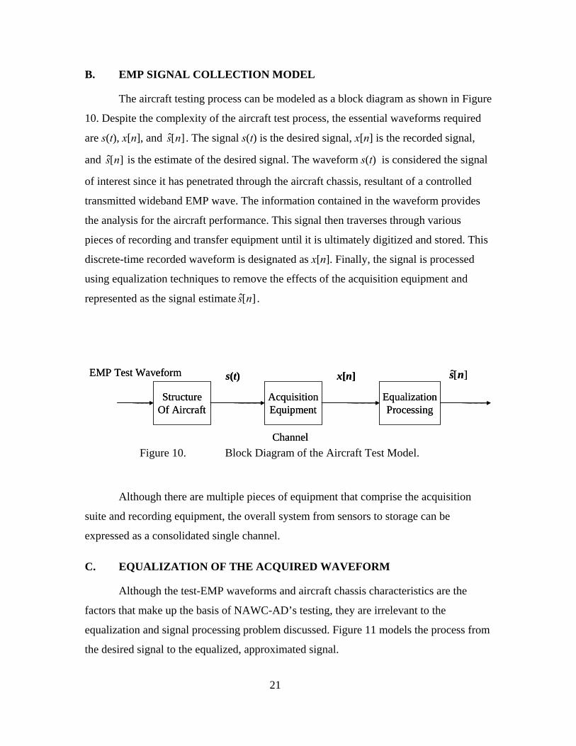
B. EMP SIGNAL COLLECTION MODEL

The aircraft testing process can be modeled as a block diagram as shown in Figure

10. Despite the complexity of the aircraft test process, the essential waveforms required

are s(t), x[n], and ˆ[ ]s n . The signal s(t) is the desired signal, x[n] is the recorded signal,

and ˆ[ ]s n is the estimate of the desired signal. The waveform s(t) is considered the signal

of interest since it has penetrated through the aircraft chassis, resultant of a controlled

transmitted wideband EMP wave. The information contained in the waveform provides

the analysis for the aircraft performance. This signal then traverses through various

pieces of recording and transfer equipment until it is ultimately digitized and stored. This

discrete-time recorded waveform is designated as x[n]. Finally, the signal is processed

using equalization techniques to remove the effects of the acquisition equipment and

represented as the signal estimate [ ]s n .

EMP Test Waveform

s(t)StructureOf Aircraft

AcquisitionEquipment

EqualizationProcessing

s(t) x[n]

Channel

ˆ[ ]s nEMP Test Waveform

s(t)StructureOf Aircraft

AcquisitionEquipment


s(t) x[n]

Channel

ˆ[ ]s n

Figure 10. Block Diagram of the Aircraft Test Model.

Although there are multiple pieces of equipment that comprise the acquisition

suite and recording equipment, the overall system from sensors to storage can be

expressed as a consolidated single channel.

C. EQUALIZATION OF THE ACQUIRED WAVEFORM

Although the test-EMP waveforms and aircraft chassis characteristics are the

factors that make up the basis of NAWC-AD’s testing, they are irrelevant to the

equalization and signal processing problem discussed. Figure 11 models the process from

the desired signal to the equalized, approximated signal.

22

Due to the nature of the comparison, it is not necessary to represent s(t) as a continuous

waveform for the system. The equipment and the signal processing techniques are digital

and discrete, and it is assumed that the sampling losses of s(t)are built into the NAWC-

AD evaluation criteria. As a result, s(t) in this system is best represented as a sampled

waveform s[n] with sampling time Ts where [ ] ( )ss n s nT= .

s[n]

Channel EqualizationFilters

x[n]s[n] [ ]s ns[n]

Channel EqualizationFilters

x[n]s[n] [ ]s n

Figure 11. Equalization Model.

The channel and the equalization filter can both be represented as systems with

response information as discussed in Chapter II. The channel characteristics are given

quantities based on equipment specification and test results. The channel information is

provided by NAWC-AD in the frequency-domain and will be as denoted as H(ω). From

this a priori knowledge of the channel, it is possible to construct an equalization filter,

G(ω) to counteract the effects of the recording equipment. Applying the discussion from

Chapter II, it can be shown that

( ) ( ) ( )

ˆ( ) ( ) ( ) ( ) ( ) ( )

X S H

S X G S H G

ω ω ω

ω ω ω ω ω ω

=

= = (3.1)

Consequently, in order to ideally equalize the system such that ˆ( ) ( )S Sω ω= , we

desire 1( )( )

GH

ωω

= . Using this relationship and the provided channel response H(ω)

from NAWC-AD, it was possible to derive a G(ω) for experimentation. In discrete-time,

this vector must have uniform frequency distribution as well as be of the same length as

the signal vector. Both these conditions were required to be met through pre-processing

due to the format of the H(ω) information discussed later.

23

D. MEASURED SIGNAL CHARACTERISTICS

Unfortunately, it is not possible to gather information on s(t) because it is the true,

unsampled, and unrecorded signal. Only x[n] can be made available since it is the

recorded signal at the aircraft test points; therefore, it is necessary to use a representative

signal for the purposes of signal analysis.

The given acquired signal, x[n], is sampled with a fixed sampling rate in the range

of 250 MHz to 1.5 GHz, dependent upon the equipment used. The waveform is a real-

valued signal and varies in length between 9,000 and 25,000 points per vector. As a

result, s[n] and [ ]s n will have the same discrete characteristics as x[n]. Visually, the

signal reflects the shape of a transient waveform as seen in Figure 12 (a) though (d). The

reader may note that the waveform shape is not consistent as is a function of the location

of test points within the aircraft.

Time in sec(a)

Time in sec(c)

Time in sec(b)

Time in sec(d)

Am

plitu

deA

mpl

itude

Am

plitu

deA

mpl

itude

Time in sec(a)

Time in sec(c)

Time in sec(b)

Time in sec(d)

Am

plitu

deA

mpl

itude

Am

plitu

deA

mpl

itude

Figure 12. Example Recorded Waveforms at Various Aircraft Test Points. (a)

Waveform 1. (b) Waveform 2. (c) Waveform 3. (d) Waveform 4.

24

There appears to be a low level of additive noise in the recorded signal x[n]. It is

not evident whether if this noise is equipment noise or background noise resident during

the radiating of the aircraft. Accordingly, the recorded signal can be represented as either

[ ] [ ]* [ ] [ ]x n s n h n w n= +

or

[ ] ( [ ] [ ])* [ ]x n s n w n h n= + .

This noise is present in the recorded signal but may not be part of the signal s[n]. It is

assumed that the noise is undesirable and not part of the ideal system; therefore, the

results could be more accurate if it were not present.

E. MEASURED CHANNEL RESPONSE

Provided by NAWC-AD were frequency responses for the acquisition equipment

used in collecting the EMP signals. The length of the equipment’s channel vectors varied

from 800-1,200 points with frequency values spanning from 200 MHz up to 1 GHz. The

channel response is complex-valued, and the frequencies do not have uniform frequency

spacing conducive to Fourier processing. Each piece of equipment was sampled using

multiple sampling frequencies and each channel was sampled in different sampling

patterns.

In Figure 13, (a) and (c) illustrate two different channel spectra provided by

NAWC-AD. The spectrum in Figure 13(a), “8694.cal,” is a vector of 1196 magnitude

values across a range of 1 GHz. The minimum spacing between these frequencies was 28

Hz, with the maximum difference being 4.166 MHz. Figure 13(b) illustrates the

irregularity of sampling by plotting the difference in frequencies between each successive

frequency values across the entire H(ω) vector. It appears that there is a step like

sampling pattern based upon the location in the frequency spectrum. Similarly, Figure

13(c) illustrates the H(ω) characteristics for the “wbal.cal” vector which is made up of

1196 frequency values. It has differences in frequency spacing ranging from 5 Hz to 2.79

MHz, although its behavior is exponential in shape as seen in Figure 13(d).

25

As discussed in Chapter II, discrete channel responses have equal and uniform

spacing throughout the spectral range of interest such that there can be a one-to-one

correspondence with the time domain. Also, the given channel frequency response

represents only the positive frequencies from 0 ω π≤ ≤ . Lastly, the measured channel

response provided is sparsely defined where 800-1,200 discrete points represent an entire

1GHz bandwidth.

0 500 10000.9

0.92

0.94

0.96

0.98

1

0 500 10000

1

2

3

4

5

50 100 1500.4

0.42

0.44

0.46

0 200 400 600 8000

1

2

3

Mag

nitu

deM

agni

tude

Frequency (MHz)(c)

Frequency Index(d)

Frequency (MHz)(a)

Frequency Index(b)

Diff

eren

ce in

Fre

quen

cy (M

Hz)

Bet

wee

n A

djac

ent P

oint

sD

iffer

ence

in F

requ

ency

(MH

z)B

etw

een

Adj

acen

t Poi

nts

0 500 10000.9

0.92

0.94

0.96

0.98

1

0 500 10000

1

2

3

4

5

50 100 1500.4

0.42

0.44

0.46

0 200 400 600 8000

1

2

3

Mag

nitu

deM

agni

tude

Frequency (MHz)(c)

Frequency Index(d)

Frequency (MHz)(a)

Frequency Index(b)

Diff

eren

ce in

Fre

quen

cy (M

Hz)

Bet

wee

n A

djac

ent P

oint

sD

iffer

ence

in F

requ

ency

(MH

z)B

etw

een

Adj

acen

t Poi

nts

Figure 13. Channel Responses and the Sampling Rates of Channel. (a) Channel

Frequency Response of “8694.cal.” (b) Difference in Frequency Values of Successive Frequency Index Points in Channel File “8694.cal.” (c) Channel Frequency Response of “wbal.cal.” (d) Difference in Frequency Values of

Successive Frequency Index Points in Channel File “wbal.cal.”

26

As a result, there is required processing of the equipment frequency response

vectors to conform to uniform frequency spacing of the discrete Fourier domain.

Additionally, the spectrum will require having the digital frequency values

from 0π ω− ≤ ≤ . As a note, irregular sampling rates can be advantageous if gathered

appropriately for a few reasons. Since Fourier transforms require uniform sampling rates

throughout the spectrum, high sampling frequencies and wide bandwidths can take up

large amounts of storage as well as require significant amounts of processing time. There

is the potential to exploit these multi-rate characteristics in a more optimal manner to

support using wavelet techniques versus Fourier transforms.

F. SIGNAL PRE-PROCESSING

There are three types of pre-processing that NAWC-AD performed prior to

equalization. These are signal extraction, DC bias removal, and linear interpolation of

channel characteristics. Before it can be determined whether more effective methods can

be employed, existing processes must be discussed.

1. Signal Extraction

The technique of signal extraction in the time domain is utilized such that signal

processing only occurs on information where the signal is present. There is the potential

for adversely impacting the information by utilizing a portion of data in which only noise

is present. Accordingly, it is beneficial to eliminate recorded information that doesn’t

contain the signal both before and after an EMP signal pulse. Signal extraction is done by

NAWC-AD in the time domain through manual processing and through visual inspection

of the recorded waveform. In each case, the information preceding the signal impulse is

manually removed by the operator, and the data at the end of the recorded waveform are

removed after it appears as though no signal is present in the recorded information. This

method eliminates consistency from the test and evaluation process because it is manual

and relies on a user interface decision. In this manner, often the same data can produce

varying degrees of processing effectiveness due to the proficiency of the operator.

For a signal with no noise, it will have no average energy where the signal is not

present and a positive value of energy wherever the signal is present. Any additive white

27

noise theoretically will create a noise floor. The average energy for a signal over a given

data length interval can be found as shown

0

2

1

1[ ] [ ]AVi N

E n x n iN = −

= −∑ (3.2)

where N is length of the signal vector. In portions where the signal is present, the average

energy of the signal is additive to the noise floor.

In order to perform this in an automated manner, it was necessary to determine a

threshold value that determines where the signal begins and where it ends. The threshold

is calculated based on the average energy found at the beginning and end of the measured

signal. For this algorithm to be successful, it must be assumed and required that there is

no signal at the beginning or end of the measured signal.

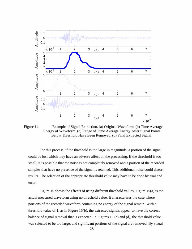
Figure 14 (a) shows a sample waveform that has been recorded, that has sample

values at the start and end of the information that do not contain the desired signal. When

the average energy is calculated and plotted, as shown in 14(b), the noise floor can be

noted at the start and end of the signal energy, and the location of the actual signal is

evident. When extraction techniques are applied to the average energy plot, as shown in

14(c), by using a threshold value, the portions of the signal assumed to have no signal

elements are removed, leaving only the length of the information containing the signal.

Lastly, 14(d) shows the extracted signal with non-signal portions removed.

28

1 2 3 4 5 6 7

x 10-6

-0.10

0.1

1 2 3 4 5 6 7

x 10-6

12345

x 10-3

1 2 3 4 5 6 7

x 10-6

0

5x 10-3

1 2 3 4 5 6 7

x 10-6

-0.10

0.1

Am

plitu

deA

mpl

itude

Am

plitu

deA

mpl

itude

(a)

(b)

(c)

(d)

1 2 3 4 5 6 7

x 10-6

-0.10

0.1

1 2 3 4 5 6 7

x 10-6

12345

x 10-3

1 2 3 4 5 6 7

x 10-6

0

5x 10-3

1 2 3 4 5 6 7

x 10-6

-0.10

0.1

Am

plitu

deA

mpl

itude

Am

plitu

deA

mpl

itude

(a)

(b)

(c)

(d)

Figure 14. Example of Signal Extraction. (a) Original Waveform. (b) Time Average Energy of Waveform. (c) Range of Time Average Energy After Signal Points

Below Threshold Have Been Removed. (d) Final Extracted Signal.

For this process, if the threshold is too large in magnitude, a portion of the signal

could be lost which may have an adverse affect on the processing. If the threshold is too

small, it is possible that the noise is not completely removed and a portion of the recorded

samples that have no presence of the signal is retained. This additional noise could distort

results. The selection of the appropriate threshold value may have to be done by trial and

error.

Figure 15 shows the effects of using different threshold values. Figure 15(a) is the

actual measured waveform using no threshold value. It characterizes the case where

portions of the recorded waveform containing no energy of the signal remain. With a

threshold value of 1, as in Figure 15(b), the extracted signals appear to have the correct

balance of signal removal that is expected. In Figures 15 (c) and (d), the threshold value

was selected to be too large, and significant portions of the signal are removed. By visual

29

inspection, a threshold value close to 1 appears to be optimum for this waveform as it is

extracting the entire signal present in the data with the potions of the noise removed.

(a)

(b)

(c)

(d)

Am

plitu

deA

mpl

itude

Am

plitu

deA

mpl

itude

(a)

(b)

(c)

(d)

Am

plitu

deA

mpl

itude

Am

plitu

deA

mpl

itude

Figure 15. Signal with Varying Levels of Energy Threshold Values. (a) Threshold =

0.1. (b)Threshold = 1. (c) Threshold = 20. (d) Threshold = 80.

2. DC Bias Cancellation

System electrical components may contain a DC bias in their equipment that

would shift the values of the entire waveform. This is an undesired effect of the

acquisition electronic equipment and may be removed. The technique of averaging is

performed to eliminate the effects of the DC bias in system equipment. In an environment

where no signal is present, it is assumed that the average value of energy would be zero

as it is with white noise. When signals travel though electronic equipment, an artificial

DC gain can manifest itself onto the signal. DC averaging is the technique to determine

that value such that it can be removed from all the data. The current method that NAWC-

30

AD uses for DC averaging is to take the first 20-150 waveform values of the recorded

signal and compute the average value of these points. This value is then removed from all

signal sample values.

As far as the experiments are concerned, it was not possible to verify whether the

cancellation of DC bias actually improved performance. Because the DC bias is

introduced into the channel in the acquisition suite, the noise contribution would need to

be artificially added, only to be removed. With no true signal s[n] available, it is not

possible to verify this improvement. Therefore, there are no results provided for this

topic.

3. Linear Interpolation of the Channel Frequency Response

As mentioned, the channel response is provided in non-uniform sampling

intervals. In order to provide equalization of the discrete waveforms in the method

discussed above, both the signal vector and the channel must have an equal number of

points and the same digital frequency in order to perform processing. In the channel

information‘s raw form, there is a disparity between the length of the signal vectors and

the channel frequency response. Therefore, the channel response requires preprocessing

before it can be applied to the signal.

It is necessary to fill the channel spectrum with magnitude values for each of the

data frequency intervals or bins. This is accomplished through linear interpolation of the

channel response. A uniformly sampled data set of length N, sampled at a rate of Fs, will

have an FFT of length N with frequency bins spaced Fs/N Hz apart. The channel

responses for the given equipment do not have such a uniform sampling as described

above.

In order to equalize the measured waveform, a magnitude value must be found for

the channel response at each discrete frequency of the data. As shown in Figure 16, a

magnitude is linearly interpolated from successive points in the channel frequency

response for frequency values dictated by the measured EMP waveform frequency bins.

This process is iterated for each FFT frequency bin so that the resultant channel response

will have an equal number of points with corresponding magnitude values at each

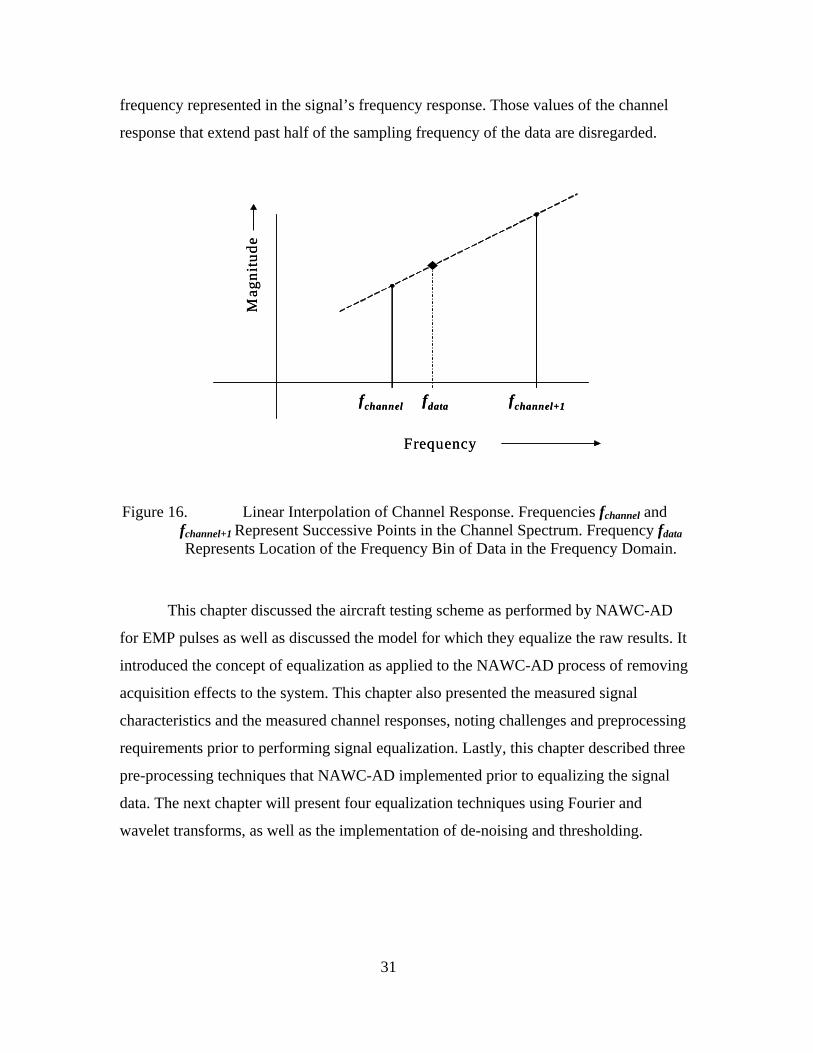
31

frequency represented in the signal’s frequency response. Those values of the channel

response that extend past half of the sampling frequency of the data are disregarded.

fchannel fchannel+1fdata

Mag

nitu

de

Frequency

fchannel fchannel+1fdata

Mag

nitu

de

Frequency

Figure 16. Linear Interpolation of Channel Response. Frequencies fchannel and fchannel+1 Represent Successive Points in the Channel Spectrum. Frequency fdata Represents Location of the Frequency Bin of Data in the Frequency Domain.

This chapter discussed the aircraft testing scheme as performed by NAWC-AD

for EMP pulses as well as discussed the model for which they equalize the raw results. It

introduced the concept of equalization as applied to the NAWC-AD process of removing

acquisition effects to the system. This chapter also presented the measured signal

characteristics and the measured channel responses, noting challenges and preprocessing

requirements prior to performing signal equalization. Lastly, this chapter described three

pre-processing techniques that NAWC-AD implemented prior to equalizing the signal

data. The next chapter will present four equalization techniques using Fourier and

wavelet transforms, as well as the implementation of de-noising and thresholding.

32


33

IV. EQUALIZATION METHODS AND WAVELET SCHEMES

The previous chapters discussed the system and parameters pertinent to measured

EMP waveforms and the channel as well as pre-processing and equalization techniques

that may be applied to processing the measured information. Three different equalization

methods were designed to process the recorded EMP-signals using wavelet transforms to

acquire results. The EMP signals were also processed using the Fourier transform

method currently used by NAWC-AD for comparison. This chapter details the algorithms

and steps taken to equalize the waveforms and to reconstruct the signal received at the

aircraft test-points.

A. EQUALIZATION

Using the principles described in Chapter II and the knowledge of the system, a

system model was required to simulate the channel and filters. Using recorded data from

NAWC-AD, it was possible to implement a model of the aircraft testing and recording

system in MATLAB and apply wavelet-based signal processing techniques in place of

those currently used by NAWC-AD. The remainder of this chapter summarizes the

techniques employed for this analysis.

1. Equalization using Wavelets

To implement equalization using wavelet transforms and perform filtering at the

sub-band level, a generic model of the system was required to employ wavelet techniques

as shown in Figure 17. The process requires wavelet decomposition, followed by

filtering, and then synthesis of the filtered waveform.

ChannelEqualization

s[n] x[n] ˆ[ ]s nWaveletDecomposition

WaveletReconstructionChannel

Equalizations[n] x[n] ˆ[ ]s nWavelet

DecompositionWavelet

Reconstruction

Figure 17. System model using Wavelet Processing for Equalization.

34

Focusing on the equalization process, a filter bank structure as shown in Figure 18

illustrates the equalization process. The input signal x[n] is decomposed into sub-band

components using the filters h′ and g′ discussed in Chapter II, filtered for equalization,

and then reconstructed into [ ]s n . Each individual filter lengths of equalization filters 1-4

are matched to the length of sub-band signals for processing. All filters were developed

and implemented using MATLAB.

EqualizationFilter 1




h' 2

g' 2

h' 2

g' 2

h' 2

g' 2

h 2

g 2h 2

g 2h 2

g 2

x[n] [ ]s nEqualization

Filter 1Equalization

Filter 2



h' 2

g' 2

h' 2

g' 2

h' 2

g' 2

h 2

g 2h 2

g 2h 2

g 2

x[n] [ ]s nEqualization

Filter 1Equalization

Filter 2



h' 2

g' 2

h' 2

g' 2

h' 2

g' 2

h 2

g 2h 2

g 2h 2

g 2

x[n] [ ]s n

Figure 18. Structure of Wavelet Analysis and Synthesis with Equalization Filtering.

The measure of system performance for the purpose of comparing the algorithms

developed in this chapter, the Mean Squared Error (MSE) between the desired

waveforms s[n] and the estimated waveform [ ]s n , is computed as [9]

[ ] [ ]( )21

MS0

1 ˆN

n

s n s nN

ε−

=

= −∑ (4.1)

where N is the numbers of signal values, and the desired waveform, s[n], is compared

against the estimated signal, ˆ[ ]s n . Mean squared error is one of many possible measures

of comparison, but it is the only one utilized to compare the results of the experiments

reported here.

2. Equalization Techniques

Three algorithms were derived to accomplish this equalization processing. All

techniques were based on wavelet decomposition of recorded EMP waveforms, but

35

varied in types of wavelet functions, filter orders, and preprocessing techniques. The

three best performing methods, as well as the technique used by NAWC-AD, were

evaluated and compared. The fourth method is the model of equalization employed by

NAWC-AD.

a. Method 1 - Time Domain Filtering of Sub-band Time Domain Signals with Inverse IIR Filter

The first method of equalization is an algorithm that decomposes the EMP

signal x[n] into sub-band time domain signals, and filters each sub-band signal by an IIR

filter constructed using the Yule-Walker method having the form ( )( )

A zB z

.

As shown in Figure 19, the recorded EMP signal, x[n], is decomposed

using the DWT into approximation and detail coefficients. Each set of coefficients is then

selectively reconstructed as discussed in Chapter II into time domain sub-band signals of

appropriate length and sampling frequency of the data. These multiple signals are then

filtered and equalized in the time domain. The resultant time-domain sub-band signals are

decomposed back into their respective coefficients, and then reconstructed back into a

full spectrum time domain signal. During decomposition, sub-band coefficients outside

the filtered sub-bands are discarded and coefficients are set to zero.

EqualizationUsing

IIR Filter

x[n] ˆ[ ]s nWaveletDecomposition

WaveletReconstructionSelective

Reconstruction

Sub-bandWavelet

Decomposition

EqualizationUsing

IIR Filter

EqualizationUsing

IIR Filter

…

EqualizationUsing

IIR Filter


WaveletReconstructionSelective

Reconstruction

Sub-bandWavelet

Decomposition

EqualizationUsing

IIR Filter

EqualizationUsing

IIR Filter

…

Figure 19. Method 1: Processing of Signal Waveforms Using Wavelet-Based

Techniques.

36

b. Method 2 – Frequency Domain Filtering using Channel Frequency Response

The second method of equalization occurs in the frequency domain versus

the time domain. Like Method 1 (see Figure 20), the algorithm decomposes the signal

into coefficients and reconstructs the sub-band signals into the time domain. It then takes

the Fourier transform of each sub-band signal and then filters each sub-band signal by

dividing the frequency response of the channel. The resultant frequency domain signals

are transformed back to the time domain using the inverse Fourier transform, where the

time-domain sub-band signals are decomposed into wavelet coefficients. The respective

coefficients are then used to reconstruct the complete signal back to the time domain.

FFTx[n]

ˆ[ ]s n

WaveletDecomposition

WaveletReconstruction

Inverse ChannelResponse Equalization

SelectiveReconstruction

FFT

FFT

…



…

IFFT

IFFT

IFFT

Sub-bandWavelet

Decomposition

FFTx[n]

ˆ[ ]s n




SelectiveReconstruction

FFT

FFT

…



…

IFFT

IFFT

IFFT

Sub-bandWavelet

Decomposition


Techniques, and Fourier Transforms.

c. Method 3 - Time Domain Filtering of Wavelet Coefficients using Inverse IIR Filter

The third algorithm, as shown in Figure 21, decomposes the EMP signal

x[n] into wavelet approximation and detail coefficients. Then each of the sub-band filter

coefficient sets is filtered by the IIR equalization filter ( )( )

A zB z

designed based on the

channel response information. The signal is then reconstructed using the sub-band

coefficients. The difference between this procedure and that of Method 1 is that the

37

coefficients are not selectively reconstructed back to their time domain forms. The

signal’s sub-band components of variable lengths are filtered accordingly.


WaveletReconstruction…

EqualizationUsing IIR Filter




WaveletReconstruction…





Techniques and IIR Filtering.

d. Method 4 – NAWC-AD Method

The NAWC-AD method filters the recorded signal, x[n], in the time

domain by using the vector multiplication of the channel’s inverse response as shown in

Figure 22. The time domain signal is then recovered by using the IFFT. This method was

discussed in Chapter II.

x[n] ˆ[ ]s nFFT IFFT

EqualizationUsing

Inverse ChannelResponse

x[n] ˆ[ ]s nFFT IFFT

EqualizationUsing

Inverse ChannelResponse

Figure 22. Method 4: Processing of Signal Waveforms Using Fourier Based Transforms as Performed by NAWC-AD.

38

B. SUB-BAND FILTERING AND NOISE REMOVAL

Although de-noising is a powerful technique available using wavelet transforms, a

detailed evaluation was not explored in this thesis. However, as a demonstration of de-

noising techniques, a soft thresholding de-noising filter using a threshold based on Stein’s

unbiased risk calculations (provided by MATLAB) was applied at each sub-band to

produce results for comparison. As shown in Figure 23, the process for de-noising occurs

after signal decomposition and before equalization. The threshold calculation noted

above is standard across the entire signal.

Equalizationx[n] ˆ[ ]s n


Denoising


s[n]

Channel EqualizationDenoising

EqualizationDenoising

…Equalization

x[n] ˆ[ ]s nWavelet

Decomposition

Denoising


s[n]

Channel EqualizationDenoising

EqualizationDenoising

…

Figure 23. De-noising Model for Processing EMP Waveforms.

Further investigation would be necessary to determine the best method for each

given channel, signal type, and wavelet basis function.

1. System Model with Additive White Gaussian Noise

To further analyze the proposed equalization techniques, an investigation was

conducted into the performance of these Fourier and wavelet transform methods when

there is noise present. A system model with additive white Gaussian noise of varying

levels added to the signal was developed as shown in Figure 24. Noise is introduced into

the system by adding it to the recorded signal, x[n].

39

s(t)AcquisitionEquipment


s(t) x[n] [ ]s ny[n]

w[n]

s(t)AcquisitionEquipment


s(t) x[n] [ ]s ny[n]

w[n] Figure 24. System Diagram with the Addition of White Noise, w[n].

Using different methods of equalization described above, the resultant waveform

[ ]s n was compared to the original noise-free waveform over a wide range of w[n] power

levels. This further expands the analysis of this experiment by comparing the

performance of the algorithms in noise-free and noisy environments and will be further

discussed as part of the results in Chapter V.

This chapter provided the specific models that were implemented to verify

whether or not wavelet-based methods could outperform existing methods. It outlined

methods and configurations used for equalization. Finally, it addressed wavelet

thresholding and the potential for data de-noising. The next chapter documents the results

of the system simulations and experimental results.

40


41

V. SIMULATION RESULTS

The previous chapters discussed many of the signal processing principles and

techniques that apply to the NAWC-AD EMP waveform processing. An experiment was

defined in order to test proposed alternative techniques. The experiment was conducted

with five types of wavelets using the four methods discussed in Chapter IV. Comparison

between three and five levels of wavelet decomposition was used since early

experimental analysis showed that performance degraded as the number of levels

exceeded five. Additionally, each set of data was processed using signal extraction and

de-noising techniques as well. This chapter presents results that characterize

performance of the various techniques compared to the present method of signal

processing. As discussed in Chapter IV, the measure of performance is the mean squared

error between the input data and the equalized estimate of the measured EMP signal.

Since the FFT-based NAWC-AD technique, Method 4, is the currently used method for

processing the EMP signals, all proposed techniques will be measured against it.

There were two primary experiments conducted for this thesis. The first involved

a comparison of the different wavelet-based techniques for equalization of the system

with the given signal information provided by NAWC-AD. The second experiment

investigated the performance of these methods with the addition of additive noise.

A. SIMULATION MODEL FOR ANALYSIS OF SYSTEM WITH NO ADDITIVE NOISE

There were two models used for analysis in the experiment. All models employed

an IIR filter representing the acquisition equipment channel constructed from the channel

frequency response information provided by NAWC-AD. The filter is implemented in

time domain to keep uniformity in its implementation. Figure 25 depicts the basic process

of the experiment.

42

s(t)IIR Filter

Method 1-4EqualizationProcessing

s[n] x[n] [ ]s n

s(t)IIR Filter


s[n] x[n] [ ]s n

Figure 25. Basic Model of System Experiment.

In addition, as described in Chapter III, the technique of signal extraction was

noted as a mechanism of improving performance and is incorporated into the model as

can be seen in Figure 26.

s(t)IIR Filter


s[n] x[n] [ ]s n

Signal Extraction

s(t)IIR Filter


s[n] x[n] [ ]s n

Signal Extraction

Figure 26. Basic Model of System Implementing Signal Extraction Technique.

Each of these models supports analysis of different types of wavelets processing

techniques against the Fourier transform based processing, as well as performance

comparison of different wavelets against each other. The signal used for all experiments,

with exception to a waveform to waveform comparison discussed below, used Waveform

1 depicted in Figure 12(a). The types of wavelets used in the process were arbitrarily

selected and are Haar, Meyer, Coiflet, Daubechie’s Order 3, and Daubechie’s Order 15

filters. In this experiment, 3-5 levels of wavelet decomposition were evaluated as it was

noted during experimentation that they provided the best results. Mean Squared Error

(MSE) as defined in Chapter IV was the basis of comparison. The technique of de-

noising is compared in each model; de-noising occurs as a function after the signals have

been decomposed into wavelet sub-bands. A comparison of these results will follow for

each model.

43

1. Equalization with No Signal Extraction

The first set of results is the comparisons of the mean squared error values with

no de-noising as shown in Figure 25. It is a direct comparison of wavelet methods,

Methods 1-3, against the Fourier transform technique, Method 4, using different wavelet

basis functions and various levels of decomposition. As noted, Waveform 1, a wideband

waveform of 16,384 points, was used following the process model of Figure 25 without

signal extraction. Each of the four methods of equalization was discussed in Chapter IV,

and wavelet decomposition is provided to the 3rd, 4th and 5th levels. The channel

frequency response used in these models was based on “8694.cal” depicted in Figure

13a. It is a 1,196-point Fourier domain response, non-linearly spaced, from 0-1GHz. This

response, therefore, required linear interpolation of its frequency values as discussed in

Chapter III, Section F. Additionally, the mean squared error values are expressed in

decibels (dB) since the absolute values are relatively small. Results of these simulations

can be seen in Table 1.

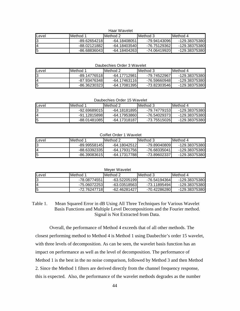
44

Haar WaveletLevel Method 1 Method 2 Method 3 Method 43 -89.62654218 -64.18408051 -79.94143096 -129.383753804 -88.02121882 -64.18403540 -76.75129362 -129.383753805 -86.68836043 -64.18404263 -74.06419920 -129.38375380

Daubechies Order 3 WaveletLevel Method 1 Method 2 Method 3 Method 43 -89.14776518 -64.17712981 -79.74522967 -129.383753804 -87.93476348 -64.17463116 -76.59660948 -129.383753805 -86.36230323 -64.17081395 -73.82303546 -129.38375380


Coiflet Order 1 WaveletLevel Method 1 Method 2 Method 3 Method 43 -89.99558145 -64.18042512 -79.89040809 -129.383753804 -88.63392335 -64.17931756 -76.68335041 -129.383753805 -86.39083615 -64.17317788 -73.89602337 -129.38375380

Meyer WaveletLevel Method 1 Method 2 Method 3 Method 43 -78.08774551 -63.52205199 -76.54194364 -129.383753804 -75.06072253 -63.03518563 -73.11895494 -129.383753805 -72.76247718 -62.46281427 -70.42286280 -129.38375380

Table 1. Mean Squared Error in dB Using All Three Techniques for Various Wavelet Basis Functions and Multiple Level Decompositions and the Fourier method.

Signal is Not Extracted from Data.

Overall, the performance of Method 4 exceeds that of all other methods. The

closest performing method to Method 4 is Method 1 using Daubechie’s order 15 wavelet,

with three levels of decomposition. As can be seen, the wavelet basis function has an

impact on performance as well as the level of decomposition. The performance of

Method 1 is the best in the no noise comparison, followed by Method 3 and then Method

2. Since the Method 1 filters are derived directly from the channel frequency response,

this is expected. Also, the performance of the wavelet methods degrades as the number

45

of levels is increased for each of the wavelet families. As wavelet basis functions,

Daubechie’s order 15 wavelet has the best performance in Method 1, but for Methods 2

and 3 the Haar wavelet performs the best.

2. Equalization with Signal Extraction

The next set of results captures the effectiveness of the signal extraction algorithm

described in Chapter III, Section F. For consistency, Waveform 1 and channel response

“8694.cal” were used again with the same preprocessing and equalization methods as in

the above discussion. Table 2 captures the results of this comparison (same results as in

Table 1, but incorporating signal extraction in preprocessing as depicted in the model in

Figure 26).

46

Haar WaveletLevel Method 1 Method 2 Method 3 Method 43 -90.34595401 -70.62104470 -80.60305640 -124.690718644 -88.42929362 -70.62113959 -77.06934195 -124.690718645 -87.46709193 -70.62039117 -74.23882826 -124.69071864



Coiflet Order 1 WaveletLevel Method 1 Method 2 Method 3 Method 43 -92.87670574 -70.61996912 -80.48567609 -124.690718644 -91.28425462 -70.61972883 -76.97295599 -124.690718645 -88.52289832 -70.60924047 -74.05139371 -124.69071864

Meyer WaveletLevel Method 1 Method 2 Method 3 Method 43 -78.46926556 -69.20423197 -76.90477957 -124.690718644 -75.28444411 -68.17274988 -73.30868711 -124.690718645 -72.90028900 -67.11307077 -70.53191399 -124.69071864

Table 2. Mean Squared Error in dB Using All Three Techniques for Various Wavelet Basis Functions and Multiple Level Decompositions and the Fourier method

using the model in Figure 26.

Similar to the results without signal extraction (see Table 1), Method 4 produces

the most similar results between the input signal and desired signal. Additionally, using

Method 1 and Daubechie’s order 15 wavelet with three levels of decomposition provides

the best results when compared with the other methods and wavelet families. In this

noise-free environment, the signal extraction algorithm performance is slightly improved

from the non-extraction case.

47

B. SIMULATION MODEL FOR ANALYSIS OF SYSTEM WITH WHITE NOISE

The second experiment, based on the models depicted in Figures 27 and 28,

captures the performance of both the wavelet and Fourier methods as a function of the

signal-to-noise ratios (SNR); the SNR is the ratio of signal power to noise power:

∑∑

=

n

n

nw

nxSNR 2

2

][

][ (5.1)

where ][nx and ][nw are the signal and noise samples, respectively. The range of SNR

evaluated for each signal was from –30 dB to 30 dB, but for each plot, the results are

shown only for the range of interest.

s(t)IIR Filter


s[n] x[n] ˆ[ ]s n

w[n]

s(t)IIR Filter


s[n] x[n] ˆ[ ]s n

w[n] Figure 27. Basic Model of System Experiment with the Addition of White Noise.

As in the previous section, the following section will compare results with and

without signal extraction, as well as with and without de-noising. In each case, the

graphical illustrations capture the comparisons between Methods 1-3 and Method 4. The

signal and channel response used are the same as in the preceding sections: Waveform 1

and channel response “8694.cal”. With the exception of adding white noise, the signal

and channel response preprocessing steps remain the same as described above.

Additionally, the mean squared error in each plot will be expressed in dB.

48

s(t)IIR Filter


s[n] x[n] [ ]s n

w[n]

Signal Extraction

s(t)IIR Filter


s[n] x[n] [ ]s n

w[n]

Signal Extraction

Figure 28. Basic Model of System Experiment with Additive White Noise and

Implementing Signal Extraction Technique.

1. Equalization Results with Additive Noise with No Signal Extraction

The results in this section show a comparison between the extracted waveforms as

a function of the signal-to-noise ratio with additive white noise. It uses Waveform 1 and

“8694.cal” as in the last section, as well as the same algorithms described in Chapter IV.

For comparison of each method, Daubechie’s Order 3 Wavelet Level 3 was used for

wavelet decomposition for Method’s 1-3. For this section, the signal of interest is not

extracted from the complete recorded signal.

a. Results without De-Noising

In this case, the signal has not been extracted and de-noising is not applied

at the sub-band level. Among all four methods, there is little difference in performance as

seen in Figure 29 (a).

49

−5 0 5 10 15 20−50

−45

−40

−35

−30

Signal Power to Noise Power (SNR) in dB(a)

MS

E in

dB

Method 1Method 2Method 3Method 4

−5 0 5 10 15 20−5

0

5

10x 10

−3

Signal Power to Noise Power (SNR) in dB(b)

MS

E in

dB


Figure 29. No Signal Extraction and De-noising. (a) Waveform 1 with Additive

Noise Using Methods Using Daubechie’s Order 3 Wavelet Level 3. (b) Normalized Results Using Daubechie’s Order 3 Wavelet Using Level 3.

Figure 29 (b) shows a comparison of the results normalized with respect to

those of Method 4. The performance of Methods 2 and 3 have improved over that of

Method 4 for SNR less than 3 dB and 13 dB, respectively. Although the degradation in

performance of MSE of Methods 2-3 appears to exponentially increase above the 0 dB

point, it must be noted that the scale of the y-axis is on the order of thousandths of a dB.

b. Results using De-noising

When the same experiment was conducted for a signal with additive noise

and no signal extraction, but with de-noising techniques, the results are significantly

different. As can be seen in Figure 30 (a), the results with de-noising have notably

50

improved for SNR less than 17 dB. However, for SNR values greater than 17 dB, the

results do not compare closely. These results are not a significant improvement to those

above where de-noising was not implemented as the signal to noise ration of the signal

increases.

10 11 12 13 14 15 16 17 18 19 20−48

−47.8

−47.6

−47.4

−47.2

−47


MS

E in

dB


10 11 12 13 14 15 16 17 18 19 20−10

−5

0

5

10


MS

E in

dB


Figure 30. No Signal Extraction. (a) Waveform1 with Additive Noise with De-

noising Using Daubechie’s Order 3 Wavelet Level 3. (b) Normalized Results with De-noising Using Daubechie’s Order 3 Wavelet Using Level 3.

The time domain plots for this case are displayed in Figure 31 at different

stages of the processing. It illustrates the impact of additive white noise and visually

shows the results at 15 dB SNR. It also demonstrates the effect with and without de-

noising in the algorithm between the input signal, s[n], and the resultant filtered

signal, [ ]s n .

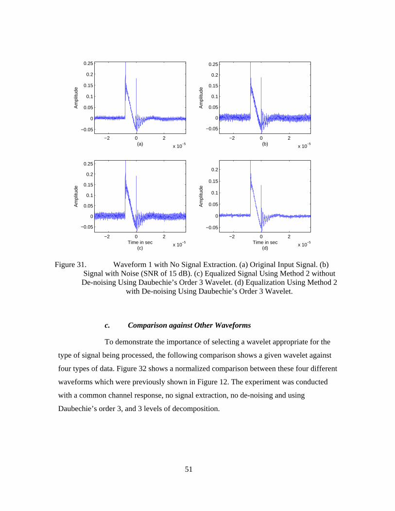
51

−2 0 2

x 10−5

−0.05

0

0.05

0.1

0.15

0.2

0.25

(a)

Am

plitu

de

−2 0 2

x 10−5

−0.05

0

0.05

0.1

0.15

0.2

0.25

(b)

Am

plitu

de

−2 0 2

x 10−5

−0.05

0

0.05

0.1

0.15

0.2

0.25

Time in sec(c)

Am

plitu

de

−2 0 2

x 10−5

−0.05

0

0.05

0.1

0.15

0.2

Time in sec(d)

Am

plitu

de

Figure 31. Waveform 1 with No Signal Extraction. (a) Original Input Signal. (b)

Signal with Noise (SNR of 15 dB). (c) Equalized Signal Using Method 2 without De-noising Using Daubechie’s Order 3 Wavelet. (d) Equalization Using Method 2

with De-noising Using Daubechie’s Order 3 Wavelet.

c. Comparison against Other Waveforms

To demonstrate the importance of selecting a wavelet appropriate for the

type of signal being processed, the following comparison shows a given wavelet against

four types of data. Figure 32 shows a normalized comparison between these four different

waveforms which were previously shown in Figure 12. The experiment was conducted

with a common channel response, no signal extraction, no de-noising and using

Daubechie’s order 3, and 3 levels of decomposition.

52

−5 0 5 10 15 20 25−0.5

0

0.5

1

1.5

2

2.5

3

3.5

4

4.5

x 10−3

Signal Power to Noise Power (SNR) in dB

MS

E in

dB

Data 1Data 2Data 3Data 4Normalized MSE

Figure 32. Comparison between Each of the Waveforms with No Signal Extraction

and Normalized MSE Values and Using Daubechie’s Order 3, and 3 Levels of Decomposition.

Figure 32 clearly shows the impact of different signals with a given

wavelet family. There is up to 10 dB of degradation in performance using the same

wavelet family, but applied to different waveforms. This observation indicates that better

performance can be achieved by selecting wavelets that correlate well to the waveforms

being processed.

2. Equalization Results with Additive Noise with Signal Extraction

The same experiment as above is repeated with signal extraction as depicted in

Figure 28, using Waveform 1, “8694.cal” as a filter response, and Daubechie’s order 3,

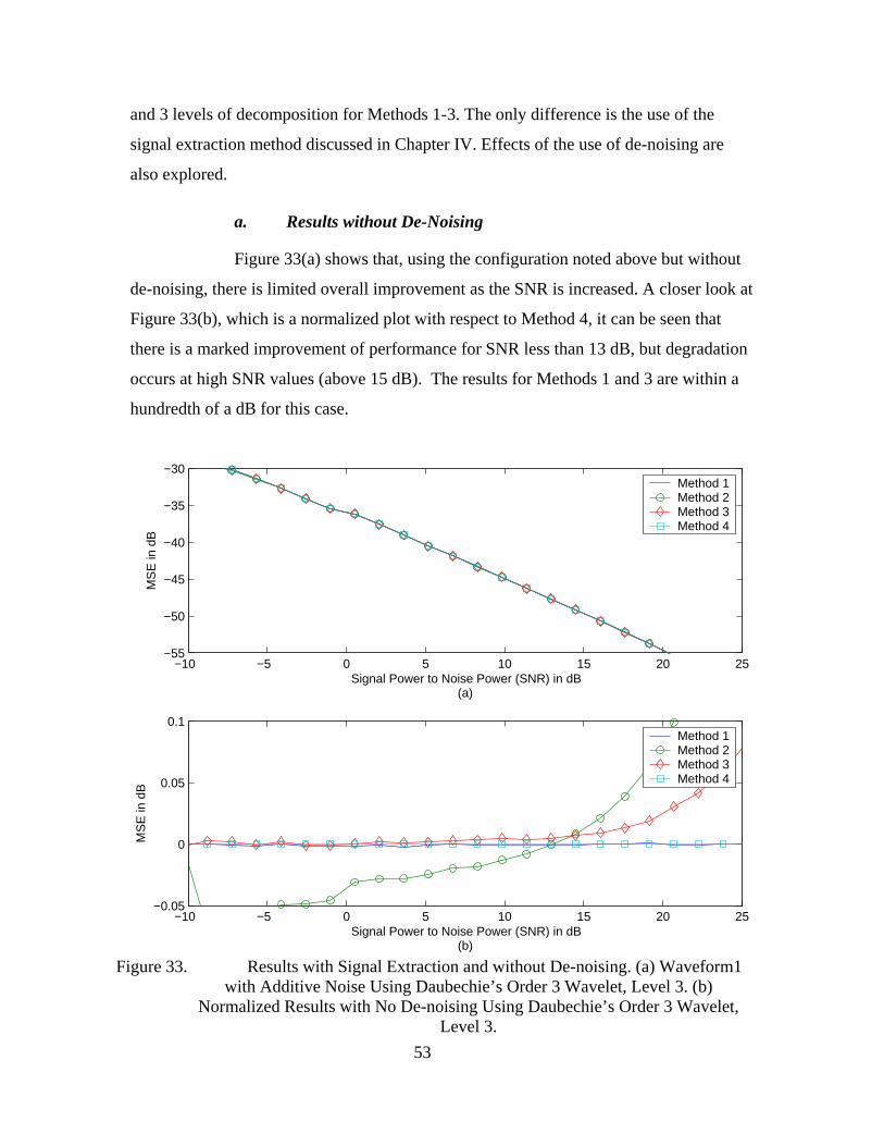
53

and 3 levels of decomposition for Methods 1-3. The only difference is the use of the

signal extraction method discussed in Chapter IV. Effects of the use of de-noising are

also explored.

a. Results without De-Noising

Figure 33(a) shows that, using the configuration noted above but without

de-noising, there is limited overall improvement as the SNR is increased. A closer look at

Figure 33(b), which is a normalized plot with respect to Method 4, it can be seen that

there is a marked improvement of performance for SNR less than 13 dB, but degradation

occurs at high SNR values (above 15 dB). The results for Methods 1 and 3 are within a

hundredth of a dB for this case.

−10 −5 0 5 10 15 20 25−55

−50

−45

−40

−35

−30


MS

E in

dB


−10 −5 0 5 10 15 20 25−0.05

0

0.05

0.1


MS

E in

dB


Figure 33. Results with Signal Extraction and without De-noising. (a) Waveform1

with Additive Noise Using Daubechie’s Order 3 Wavelet, Level 3. (b) Normalized Results with No De-noising Using Daubechie’s Order 3 Wavelet,

Level 3.

54

b. Results with De-Noising

Figure 34 shows results with de-noising and signal extraction using

Waveform 1 and “8694.cal”. It can be seen again that there is improvement in the

performance for SNR less than approximately 15dB. Compared to the results in the

previous section (see Figure 33), there was slight improvement to the performance of the

system at higher SNR values when de-noising techniques were implemented as shown in

Figure 34.

−10 −5 0 5 10 15 20 25−55

−50

−45

−40

−35

−30


MS

E in

dB


14 14.2 14.4 14.6 14.8 15 15.2 15.4 15.6 15.8 16−1

−0.5

0

0.5

1


MS

E in

dB


Figure 34. MSE as a function of SNR with Signal Extraction and De-noising: (a)

Waveform1 with Additive Noise Using Daubechie’s Order 3 Wavelet, Level 3. (b) Normalized values Using Daubechie’s Order 3 Wavelet, Level 3.

55

A last comparison, in Figure 35, shows the time domain representations of

the waveforms with a 15 dB SNR using extraction techniques. The desired signal has

been extracted from the data containing only the portion of the data where the signal is

present. The simulation parameters used to obtain the results in Figure 35 are same as

those used to obtain the results in Figure 31 with the exception that signal extraction is

applied here. As can be seen, the waveforms have been processed only over the extracted

portions.

−2 0 2

x 10−5

−0.05

0

0.05

0.1

0.15

0.2

0.25

(a)

Am

plitu

de

−2 0 2

x 10−5

−0.05

0

0.05

0.1

0.15

0.2

0.25

(b)

Am

plitu

de

−2 0 2

x 10−5

−0.05

0

0.05

0.1

0.15

0.2

0.25

Time in sec(c)

Am

plitu

de

−2 0 2

x 10−5

−0.05

0

0.05

0.1

0.15

0.2

Time in sec(d)

Am

plitu

de

Figure 35. Waveform 1 with Signal Extraction: (a) Original Input Signal. (b) Signal

with Noise (SNR of 15 dB). (c) Equalized Signal Using Method 2 without De-noising Using Daubechie’s Order 3 Wavelet. (d) Equalization Using Method 2

with De-noising Using Daubechie’s Order 3 Wavelet.

56

This chapter provided results and plots demonstrating the performance of

the algorithms described in the previous chapters. The results compared a single

waveform data set using different wavelet types. The performance of the four methods

are compared as a function of the signal-to-noise ratio (-30 to 30 dB) using wavelet de-

noising techniques. The experiments compared the difference in performance with and

without signal extraction. The conclusions of the work reported here and the results are

discussed in Chapter VI.

57

VI. CONCLUSIONS

This thesis applied wavelet-based signal processing techniques to an existing

practical problem of aircraft testing for vulnerability to EMP. It sought to investigate

whether the performance of an equalizer could be improved using wavelet decomposition

versus Fourier transform, whether sub-band de-noising, as well as preprocessing

techniques for extracting the signal from arbitrary data would prove beneficial.

A. SIGNIFICANT RESULTS

First, we analyzed whether equalization using wavelet transforms could

outperform equalization using Fourier transforms. The investigation included five

different types of wavelets and three different levels of decomposition each. Results

showed that Fourier transforms produced a closer approximation to the input signal after

equalization. This can be attributed to the fact that the data collected from the channel

was already in the frequency domain, and the scarcity of channel response data and

channel dynamics precluded a dramatic increase in performance. Although sub-band

level processing is expected to have better results, given the known channel information,

Fourier transform processing was less computationally intensive, and provided a better

approximation in low noise environments.

Second, we implemented a preprocessing algorithm to remove undesired portions

of the signal from a given signal vector using time average energy calculations. Results

showed performance improvement and a closer approximation of the desired signal using

this technique. Additionally, from a test and evaluation standpoint in order to support

acceptance and certification, it will keep the signal quality from being sensitive to

operator intervention and error.

Lastly, we investigated the equalization, signal extraction, and de-noising for a

given set of recorded signal measurements with the addition of additive noise. Results

showed that using wavelets had better performance than processing in the frequency

domain for signals with additive noise; however, the results of de-noising are preliminary

and further in-depth investigation is warranted to draw definitive conclusions on the

58

performance improvement with de-noising. For each algorithm with de-noising, the

wavelet based processing had better results for signal-to-noise ratios of less than 15 dB.

Results suggest that the current method employed by NAWCAD for channel

equalization using Fourier transforms is optimal in a low noise (high SNR) environment

based on the channel (equipment) response provided. Although potentially beneficial

with other systems, wavelet processing did not provide significant improvement to the

process at high SNRs. Additionally, it added considerable processing overhead for the

equalization process. Nevertheless, significant improvement in performance of the

proposed wavelet methods with de-noising is obtained at low SNRs, a desirable outcome

especially when the aircraft testing is conducted under noisy conditions. Results also

suggest that removing undesired portions of a signal from a given data set as part of

preprocessing provided improved system performance. By automating the signal

extraction process using the principle of time average energy, one can obtain consistency

and repeatability of the results.

B. RECOMMENDATIONS FOR FURTHER RESEARCH

In this thesis, using basic wavelet de-noising techniques there was an

improvement in signal extraction performance in high noise environments. However, the

techniques used were basic and no in-depth study was conducted. A more detailed look

into which thresholding methods would be optimum for these processes will be useful.

More detailed investigation into which wavelet families work best for these classes of

signal and channel structures could also be conducted to improve system performance.

The ability to exploit the multi-rate sampling techniques of the channel

characteristics is another viable option. Because of the compression capabilities of

wavelets, although not discussed, a multi-rate technique may be developed that could

capture more information about channel using fewer points.

Finally, the use of fractional Fourier transforms, or other linear or non-linear

transforms, may also offer an alternative method for improving the performance of this

59

system. Based on the uniqueness of the system and signal characteristics, the solution

should not be limited to wavelet or Fourier transform processing to provide the most

optimal results.

60


61

APPENDIX

A. MAIN PROGRAMS

The following section provides the MATLAB code used for the results generated

in Chapter V. It provides the code both for the Tables and plots. The succeeding section,

Section B, provides the code for the subroutines called in the following program sets.

1. Program Producing Tables for Chapter V

%%%%%%%%%%%%%%%%%%%%%%%%%%%%%%%%%%%%%%%%%%%%%%%%%%%%%%%%%%%%%%%% % % This MATLAB file is the main operating program for simulations of % signal processing for this thesis. % It is the program that implements the extraction technique on data % and presents the data with and without de-noising techniques. % The results of this program produce the Tables of Chapter V, and only % results for the original signal with no added noise. This program % primarily compares the different wavelet basis functions against % one another as well as compares the effectiveness of different levels % of decomposition % % Functions Called: % calprog2() % buildiir() % avepower() % filterNreconstruct() % polywavfil1() % wavedecom() % noisepolywavfil1() % noisewavedecom() % %%%%%%%%%%%%%%%%%%%%%%%%%%%%%%%%%%%%%%%%%%%%%%%%%%%%%%%%%%%%%%%%%%% % Clear variables and close all figures clear; close all; % Define data1 as global global data1 % Loads in data

62

loadprogdatahome; % Find length of data signal to be used n=length(data1(:,2)); % Finds the freq response of channel response data @ freq bins of input data [caldata]=calprog2(y4,deltaf1,n); % Finds IIR coefficients and IIR filter frequency response of order 40 from % the channel response data [g,biir,aiir]=buildiir(caldata(1:n/2+1,:),40,'n'); % Established full spectrum (both halves of butterfly) g1=[g' fliplr(conj(g(2:length(g')-1)'))]'; % Establishes noise contribution from the signal sigpower=var(data1(:,2)); % Establish the noise power to be added to the signal sigma=0; % Creates Data-- The vector to be filtered data=data1; % Seeds the random generator to keep results consistent for comparison randn('state',1); % Adds noise to signal data(:,2)=data1(:,2) + sigma*randn(length(data1(:,2)),1); % Finds the extraction parameters using the function avepower [dd,start,stop,data]=avepower(data); % Extracts the signal from the data and fills in zeros to match the % length of the orignal data data1(:,2)=[data1(start:stop,2); zeros(n-(stop-start+1),1)]; % Plots input data in the Time and Frequency Domain figure('name','Original Data- Time & Freq Domain'); subplot(2,1,1);plot(data1(:,1),data1(:,2),data1(:,1),data(:,2)) subplot(2,1,2);plot(f1,abs(fft(data1(:,2))),f1,abs(fft(data(:,2)))) % Creates signal x[n] that needs to be equalized % Sends input throught the channel filterout=filter(biir,aiir,data(:,2));disp('end filter');

63

% Equalizes the signal x[n] through division of the channel frequency % response. Method 4 (their method) ffout=fft(filterout); fyout=ffout./g1; % yout is shat[n] for method 4 yout=real(ifft(fyout)); % Plot of x[n] in Time Domain figure('name','Filtered Data using IIR Filter') subplot(2,1,1);plot(filterout); axis tight % Plot of x[n] in Frequency Domain subplot(2,1,2) plot((abs(ffout)));axis tight; title({['Figure 1'],['filtered output']}); % Plot of shat[n] in Frequency Domain figure('name','Equalized Output using FFT') plot(f1,abs(fyout),f1,abs(fdata1(:,2))); title({['Figure 1'],['equalized output usinf fft']}); % Initializes parameters for wavelet basis functions and levels of decomposition wavnamelist={'haar' 'db3' 'db15' 'coif1' 'dmey'}; lev=[3 4 5]; for i=1:5 wavname=wavnamelist{i}; disp(' ');disp(' '); disp(sprintf('%-10s%',wavname)) disp(sprintf('%-5s %-15s %-15s %-15s %-15s %-15s %-15s %-15s','level','Method 1','Method 2','Method 3','Present Tech','Method 1 noise','Method 2 noise','Method 3 Noise')) for j=1:3 level=lev(j); % Find Time Domain data for Approx's and Details for current % wavelet basis functions and number of levels [A,D]=wavedecom(wavname,level,filterout,'n'); % Find Time Domain data for Approx's and Details for current % wavelet basis functions and number of levels using de-noising % techniques [nA,nD]=noisewavedecom(wavname,level,filterout,'n'); % Equalize the data using Methods 1 and 2, for the with and % without de-noising methods. % NEWDATA is the equalized output using inverse IIR filter

64

% (method 1) % FFTNEWDATA is equalized output using inverse channel % frequency response (method 2) [newdata,fftnewdata]=filterNreconstruct(g1,aiir,biir,A,D,wavname); [noisenewdata,noisefftnewdata]=filterNreconstruct(g1,aiir,biir,nA,nD,wavname); % Equalization of the data Using Method 3 for the with and % without de-noising methods. [polynewdata1]=polywavfil1(aiir,biir,wavname,level,filterout); [noisepolynewdata1]=noisepolywavfil1(aiir,biir,wavname,level,filterout); % Find the Mean Squared Error of Techniques 1-3 (with and without de-noising) % in dB, using original noiseless data as comparison s1=10*log10(mean((data1(:,2)-newdata').^2)); s2=10*log10(mean((data1(:,2)-fftnewdata).^2)); s3=10*log10(mean((data1(:,2)-polynewdata1').^2)); s4=10*log10(mean((data1(:,2)-yout).^2)); s5=10*log10(mean((data1(:,2)-noisenewdata').^2)); s6=10*log10(mean((data1(:,2)-noisefftnewdata).^2)); s7=10*log10(mean((data1(:,2)-noisepolynewdata1').^2)); disp(sprintf('%-5.0f %-15.8f %-15.8f %-15.8f %-15.8f %-15.8f %-15.8f %-15.8f ',level,s1,s2,s3,s4,s5,s6,s7)) end end

2. Program that Produces Figures for Chapter V

%%%%%%%%%%%%%%%%%%%%%%%%%%%%%%%%%%%%%%%%%%%%%%%%%%%%%%%%%%%%%%%% % % This MATLAB file is the main operating program for simulations of % signal processing for this thesis. % It is the program that implements the extraction technique on data % and presents the data with and without de-noising techniques. % The results of this program produce the Figures of Chapter V, and only % results for the original signal with added noise over the range of signal- % to-noise ratio (SNR) from -15 to 30 dB. This program primarily compares the % different methods against one another for a given wavelet basis function % and fixed number of levels for wavelet decomposition % % % Functions Called:

65

% calprog2() % buildiir() % avepower() % filterNreconstruct() % polywavfil1() % wavedecom() % noisepolywavfil1() % noisewavedecom() % %%%%%%%%%%%%%%%%%%%%%%%%%%%%%%%%%%%%%%%%%%%%%%%%%%%%%%%%%%%%%%%%%%% % Clear variables and close all figures clear; close all; % Define data1 as global global data1 % Loads in data loadprogdatahome; % Find length of data signal to be used n=length(data1(:,2)); % Finds the freq response of channel response data @ freq bins of input data [caldata]=calprog2(y4,deltaf1,n); % Finds IIR coefficients and IIR filter frequency response of order 40 from % the channel response data [g,biir,aiir]=buildiir(caldata(1:n/2+1,:),40,'n'); % Established full spectrum (both halves of butterfly) g1=[g' fliplr(conj(g(2:length(g')-1)'))]'; % Conduct sweep of techniques over SNR -15 to 30dB iter=30; snr=linspace(-15,30,iter); % Initialize Mean Squared error matrices to save results mmse=zeros(7,iter); % Performs the channel filtering and equalization over the range of SNR from -15 to % 30 dB. for v=1:iter % Loads in original data loadprogdatahome;

66

n=length(data1(:,2)); close all; % Establishes noise contribution from the signal sigpower=var(data1(:,2)); % Establish the noise power to be added to the signal sigma=sqrt(sigpower/10^(.1*snr(v))); disp(['The amount of noise is: ',num2str(sigma)]); % Creates Data-- The vector to be filtered data=data1; % Seeds the random generator to keep results consistent fot comparison randn('state',1); % Adds noise to signal data(:,2)=data1(:,2) + sigma*randn(length(data1(:,2)),1); % Finds the extraction parameters using the function avepower [dd,start,stop,data]=avepower(data); % Extracts the signal from the data and fills in zeros to match the % length of the orignal data data1(:,2)=[data1(start:stop,2); zeros(n-(stop-start+1),1)]; % Plots input data in the Time and Frequency Domain figure('name','Original Data- Time & Freq Domain'); subplot(2,1,1);plot(data1(:,1),data1(:,2),data1(:,1),data(:,2)) subplot(2,1,2);plot(f1,abs(fft(data1(:,2))),f1,abs(fft(data(:,2)))) % Creates signal x[n] that needs to be equalized % Sends input throught the channel filterout=filter(biir,aiir,data(:,2)); % Equalizes the signal x[n] through division of the channel frequency % response. Method 4 (their method) ffout=fft(filterout); fyout=ffout./g1; % yout is shat[n] for method 4 yout=real(ifft(fyout)); % Plot of x[n] in Time Domain figure('name','Filtered Data using IIR Filter') subplot(2,1,1);plot(filterout); axis tight % Plot of x[n] in Frequency Domain subplot(2,1,2) plot((abs(ffout)));axis tight; title({['Figure 1'],['filtered output']});

67

% Plot of shat[n] in Frequency Domain figure('name','Equalized Output using FFT') plot(f1,abs(fyout),f1,abs(fdata1(:,2))); title({['Figure 1'],['equalized output usinf fft']}); % Initializes parameters for wavelet basis functions and levels of decomposition wavnamelist={'haar' 'db3' 'db15' 'coif1' 'dmey'}; lev=[3 4 5]; % Initialize index to choose wavelet basis function i=2; wavname=wavnamelist{i}; disp(' ');disp(' '); disp(sprintf('%-10s%',wavname)) disp(sprintf('%-5s %-15s %-15s %-15s %-15s %-15s %-15s %-15s','level','Method 1','Method 2','Method 3','Present Tech','Method 1 noise','Method 2 noise','Method 3 Noise')) % Initialize index to choose number of levels of decomposition j=2; level=lev(j); % Find Time Domain data for Approx's and Details for current % wavelet basis functions and number of levels [A,D]=wavedecom(wavname,level,filterout,'n'); % Find Time Domain data for Approx's and Details for current % wavelet basis functions and number of levels using de-noising % techniques [nA,nD]=noisewavedecom(wavname,level,filterout,'n'); % Equalize the data using Methods 1 and 2, for the with and % without de-noising methods. % NEWDATA is the equalized output using inverse IIR filter % (method 1) % FFTNEWDATA is equalized output using inverse channel % frequency response (method 2) [newdata,fftnewdata]=filterNreconstruct(g1,aiir,biir,A,D,wavname); [noisenewdata,noisefftnewdata]=filterNreconstruct(g1,aiir,biir,nA,nD,wavname); % Equalization of the data Using Method 3 for the with and % without de-noising methods. [polynewdata1]=polywavfil1(aiir,biir,wavname,level,filterout); [noisepolynewdata1]=noisepolywavfil1(aiir,biir,wavname,level,filterout); % Find the Mean Squared Error of Techniques 1-3 (with and without de-noising) % in dB, using original noiseless data as comparison s1=10*log10(mean((data1(:,2)-newdata').^2));

68

s2=10*log10(mean((data1(:,2)-fftnewdata).^2)); s3=10*log10(mean((data1(:,2)-polynewdata1').^2)); s4=10*log10(mean((data1(:,2)-yout).^2)); s5=10*log10(mean((data1(:,2)-noisenewdata').^2)); s6=10*log10(mean((data1(:,2)-noisefftnewdata).^2)); s7=10*log10(mean((data1(:,2)-noisepolynewdata1').^2)); % Display results to the screen disp(sprintf('%-5.0f %-15.8f %-15.8f %-15.8f %-15.8f %-15.8f %-15.8f %-15.8f ',level,s1,s2,s3,s4,s5,s6,s7)) % Save current iterations data to matrix mmse(:,v)=[s1 s2 s3 s4 s5 s6 s7]'; end % Plot of Mean Squared Errors of Methods over SNR from -15 to 30 dB, % Non-normalized and not using de-noising techniques figure;subplot(2,1,1) plot(snr,mmse(1,:),snr,mmse(2,:),'o-',snr,mmse(3,:),'d-',snr,mmse(4,:),'s-'); axis tight legend('Method 1','Method 2','Method 3','Present Technique') xlabel({['Signal Power to Noise Power (SNR) in dB'],['(a)']}) ylabel('MSE in dB') % Plot of Mean Squared Errors of Methods over SNR from -15 to 30 dB, % Normalized and not using de-noising techniques subplot(2,1,2) plot(snr,mmse(1,:)-mmse(4,:),snr,mmse(2,:)-mmse(4,:),'o-',snr,mmse(3,:)-mmse(4,:),'d-',snr,mmse(4,:)-mmse(4,:),'s-'); axis tight legend('Method 1','Method 2','Method 3','Present Technique') xlabel({['Signal Power to Noise Power (SNR) in dB'],['(b)']}) ylabel('MSE in dB') % Plot of Mean Squared Errors of Methods over SNR from -15 to 30 dB, % Non-normalized and using de-noising techniques figure;subplot(2,1,1) plot(snr,mmse(5,:),snr,mmse(6,:),'o-',snr,mmse(7,:),'d-',snr,mmse(4,:),'s-'); axis tight legend('Method 1','Method 2','Method 3','Present Technique') xlabel({['Signal Power to Noise Power (SNR) in dB'],['(a)']}) ylabel('MSE in dB') % Plot of Mean Squared Errors of Methods over SNR from -15 to 30 dB, % Normalized and using de-noising techniques subplot(2,1,2) plot(snr,mmse(5,:)-mmse(4,:),snr,mmse(6,:)-mmse(4,:),'o-',snr,mmse(7,:)-mmse(4,:),'d-',snr,mmse(4,:)-mmse(4,:),'s-'); axis tight

69

legend('Method 1','Method 2','Method 3','Present Technique') xlabel({['Signal Power to Noise Power (SNR) in dB'],['(b)']}) ylabel('MSE in dB')

B. FUNCTIONS USED IN ABOVE MAIN PROGRAMS

1. AVEPOWER

function [dcdrift,startIndex,stopIndex,dataExtracted]=avepower(data); %%%%%%%%%%%%%%%%%%%%%%%%%%%%%%%%%%%%%%%%%%%%%%%%%%%%%%%%%%%%%%%% % AVEPOWER % % This function takes a data sequence "data" and returns % signal extracted version of data signal % as well as the index where the signal starts, % the index where the signal stops, and the mean % of the values not contained in the signal % % Inputs: % data (data signal to be extracted) % Outputs: % dcdrift (DC Bias of non-signal data)) % StartIndex (index of original data that signal begins) % StopIndex (index of original data that signal ends) % dataExtracted (Extracted signal from data) % %%%%%%%%%%%%%%%%%%%%%%%%%%%%%%%%%%%%%%%%%%%%%%%%%%%%%%%%%%%%%%%%%%% % Establish level of performance of the Threshold. threshperf=1; % Determine length of the data n=length(data(:,1)); % Establish length of the interval to average over interval=round(n/10); % Initialize variable for energy values energy=zeros(n,1); % Find the average enrgy values over length of data. for i=1:n window=(i-(interval-1)); if (i-(interval-1))<1, window=1; end

70

energy(i)=sum(data(window:i,2).^2)/interval; end % Plot the Original data figure subplot(4,1,1) plot(data(:,1),data(:,2)); axis tight xlabel('(a)') ylabel('Amplitude') % Plot the Average energy calculation of the data subplot(4,1,2) plot(data(:,1),energy,'.-'); axis tight xlabel('(b)') ylabel('Amplitude') % Establish thresholds for the data, thresh1 represents the threshold at % the beginning of the data, thresh2 represents the data at the end of % the data string thresh1=threshperf*1.5; thresh2=threshperf*2; % Find the Beginning of the signal; where the energy crosses the threshold startIndex=interval; count=1; while (thresh1*energy(startIndex) > energy(count))&(count<n) count=count+1; end % Add portion of data to prevent unnecessary loss of the signal startIndex=(count-round(count/5)); % Find the end the signal in the data; where the end of the signal crosses % the threshold. stopIndex=n; count=n; while (thresh2*energy(n) > energy(count))&(count>1) count=count-1; end % Add portion of data to prevent unnecessary loss of the signal stopIndex=(count+round(interval/2)); % Check values to make sure they are valid if stopIndex>=n, stopIndex=n; end if startIndex<1, startIndex=1; end

71

if stopIndex<startIndex, stopIndex=n; startIndex=1; end % Eliminate portions in the average time energy profile that do not contain the signal energy=[energy(startIndex:stopIndex); zeros(n-(stopIndex-startIndex+1),1)]; % Eliminate portions of the data that does not contain portions of the signal dataExtracted(:,2)=[data(startIndex:stopIndex,2); zeros(n-(stopIndex-startIndex+1),1)]; % Calculate the average noise energy of the data not considered the signal dcdrift=mean([data(interval:startIndex,2) ;data(stopIndex:n,2)]); % Plot the extracted time average energy of the signal subplot(4,1,3) plot(data(:,1),energy); axis tight xlabel('(c)') ylabel('Amplitude') % Plot the extracted signal subplot(4,1,4) plot(data(:,1),dataExtracted(:,2)); axis tight xlabel({['Time in sec'],['(d)']}) ylabel('Amplitude')

2. CALPROG2

function [calnew]=calprog2(cal,df,nx); %%%%%%%%%%%%%%%%%%%%%%%%%%%%%%%%%%%%%%%%%%%%%%%%%%%%%%%%%%%%%%%%%% % CALPROG2 % % This function takes given channel response, % This code was modified from foldprob.m [ref] % Inputs: % cal (data signal to be extracted) % df (delta frequency of data signal) % nx (number of data points in the data signal) % Outputs: % calnew (Extracted signal from data) % Function calls: % interpjk() % extend() % unwrap() % %%%%%%%%%%%%%%%%%%%%%%%%%%%%%%%%%%%%%%%%%%%%%%%%%%%%%%%%%%%%%%%%%%%

72

% INTERPJK Table look-up. % Y = interpjk(dataset1,dataset2) returns a dataset of linearly % interpolated rows, mapping dataset1 to the first column of % dataset2. % % NOTE: dataset2's 1st column and dataset1 must be monotonically % increasing. %%%%%%%%%%%%%%%%%%%%%%%%%%%%%%%%%%%%%%%%%%%%%%%%%%%%%%%%%%%%%%%%%%% % EXTEND % dataset1=extend(dataset1,dataset2) % % Use extend to extend the data to allow for interpolation of % datasets whose points do not match up. %%%%%%%%%%%%%%%%%%%%%%%%%%%%%%%%%%%%%%%%%%%%%%%%%%%%%%%%%%%%%%%%%%% % UNWRAP Unwrap phase angle. % UNWRAP(P) unwraps radian phases P by changing absolute % jumps greater than pi to their 2*pi complement. It unwraps % along the first non-singleton dimension of P. P can be a % scalar, vector, matrix, or N-D array. % % UNWRAP(P,TOL) uses a jump tolerance of TOL rather % than the default TOL = pi. % % UNWRAP(P,[],DIM) unwraps along dimension DIM using the % default tolerance. UNWRAP(P,TOL,DIM) uses a jump tolerance % of TOL. %%%%%%%%%%%%%%%%%%%%%%%%%%%%%%%%%%%%%%%%%%%%%%%%%%%%%%%%%%%%%%%%%%% % Find the number of data points in the channel frequency response n=length(cal); % Set up frequency bins for channel response interpolation f=linspace(0,df*nx/2,nx/2+1); % Interpolates data and sets data to the scale of the vector f % Code taken from foldprob.n [ref] newdata=interpjk(cal,f); cal_id=extend(cal,f); t=[cal_id(:,1),abs(cal_id(:,2)),angle(cal_id(:,2))]; t(:,3)=unwrap(t(:,3)); ct=interpjk(t,f');

73

clear t; t=ct(:,2).*(cos(ct(:,3))+sin(ct(:,3))*i); clear cal_id; % saves modified interpolated data as newdata newdata=t'; % Takes the one-sidedspectrum and adds its complex conjugate other side if length(newdata)/2 ~= round(length(newdata)/2) fulldata=[newdata fliplr(conj(newdata(2:length(newdata)-1)))]; else fulldata=[newdata fliplr(conj(newdata(2:length(newdata))))]; end % Saves final channel response as calnew calnew=[linspace(0,(length(fulldata)-1)*df,length(fulldata))' fulldata']; % Plot of channel frequency response before and after interpolation figure('name','Channel Freq Domain- Before/ After interpolation') subplot(2,1,1) plot(cal(:,1),abs(cal(:,2)),'.') axis tight subplot(2,1,2) plot(f,abs(newdata),'.') axis tight % Plot of full spectrum of channel response and its time domain impulse % response. figure('name','Channel Freq and Time Domain') subplot(2,1,1) plot(calnew(:,1),abs(calnew(:,2))) subplot(2,1,2) ff=ifft(fulldata); plot(abs(ff)); axis([0 4000 0 .0001])

3. WAVEDECOM

function [A,D]=wavedecom(wavlet,level,data,pr); %%%%%%%%%%%%%%%%%%%%%%%%%%%%%%%%%%%%%%%%%%%%%%%%%%%%%%%%%%%%%%%%

74

% % This function finds the time domain sub-band signals, Approximation and % Detail for a given data vector "data" with "level" number of levels % decomposition and using the "wavelet" basis function. All Approximation % and Detail sub-band signals are found for all levels and are arranged % in "level" number of vectors in the A and D Matrices, respectively % % Inputs: % wavlet (Type of Wavelet basis function to be used) % level (Number of levels of decomposition) % data (Data vector to be decomposed) % pr (string variable, 'y', prints all associated plots) % Outputs: % A (sub-band Time Domain Approximation signals in matrix form of all levels) % D (sub-band Time Domain Detail signals in matrix form of all levels) % %%%%%%%%%%%%%%%%%%%%%%%%%%%%%%%%%%%%%%%%%%%%%%%%%%%%%%%%%%%%%%%%%%% % Determine the length of the data n=length(data); % Decompose the data using above described parameters [C,L] = wavedec(data,level,wavlet); % Find the Approximation coefficients for last level of decomposition Atmp= appcoef(C,L,wavlet,level); % Zero pad the remaining length of Approximation coefficients up to length n n1=1:n/(2^level); A=[Atmp' zeros(1,n-L(1))]; % Find the Detail coefficients for all levels of decomposition Dc=detcoef(C,L,wavlet,level)'; % If requested Display the following plots if pr == 'y' % Plot of the last level of Approximation coefficients and all levels % of Detail Coefficients figure('name','Wavelet Coefficients') subplot(2,2,1) plot(Atmp);axis tight title(['A',num2str(level),' Coefficients']) subplot(2,2,2)

75

plot(Dc{level});axis tight title(['D',num2str(level),' Coefficients']) subplot(2,2,3) plot(Dc{level-1});axis tight title(['D',num2str(level-1),' Coefficients']) subplot(2,2,4) plot(Dc{level-2});axis tight title(['D',num2str(level-2),' Coefficients']) for i=1:level-3 if mod(i-1,4)==0 figure('name','Wavelet Coefficients') end subplot(2,2,mod(i-1,4)+1); plot(Dc{level-(i+2)}); axis tight title(['D',num2str(level-(i+2)),' Coefficients']) end % Plot of Original Signal figure('name','Original data') plot(data);axis tight end % Initialize matrices A=zeros(level,n); D=zeros(level,n); % For each level of decomposition save the selective reconstruction of the % Approximation and Detail Time Domain signals for i=1:level A(i,:) =wrcoef('a',C,L,wavlet,i)'; D(i,:) = wrcoef('d',C,L,wavlet,i)'; end % If requested, display, the following plots of Time domain sub-band % signals for all Approximation and Detail levels of decomposition if pr=='y' for i=1:level if mod(i-1,4)==0 figure('name','Wavelet Time Domain Approximations and Details') end subplot(4,2,mod(2*(i-1),8)+1); plot(A(i,:)); axis tight title(['A',num2str(i),' Reconstruction to Time Domain']) subplot(4,2,mod(2*(i-1),8)+2); plot(D(i,:)); axis tight

76

title(['D',num2str(i),' Reconstruction to Time Domain']) end end

4. BUILDIIR

function [g,b,a]=buildiir(cal,order,pr) %%%%%%%%%%%%%%%%%%%%%%%%%%%%%%%%%%%%%%%%%%%%%%%%%%%%%%%%%%%%%%%% % BUILDIIR % % This function finds IIR filter coefficients for the best fit filter % given frequency response using a mean squared error criterion. % Yule-Walker function from MATLAB used to determine coefficients from % Frequency Response. % % Inputs: % cal (FFT of channel response) % order (Order of desired IIR filter, zero implies MMSE best fit) % pr (string variable, 'y', prints all associated plots) % Outputs: % g (Frequency Response of IIR Filter) % a (IIR Filter denominator coefficients) % b (IIR Filter numerator coefficients) % %%%%%%%%%%%%%%%%%%%%%%%%%%%%%%%%%%%%%%%%%%%%%%%%%%%%%%%%%%%%%%%%%%% % Fimd the length of channel frequency response vector n=length(cal(:,1)); % Normalize the Channel Frequencies from 0 to 1 f=cal(:,1)/cal(n,1); % Establish vestor of Channel Magnitudes m=abs(cal(:,2)); % Find the optimum filter if the input order is zero if order==0 % Initialize the comparison of the error value besterror=10^16; % Find the best filter from order 2 to 80, with even order values.

77

for i=1:40 % Find filter coefficients of order 2*i using yulewalk [b1,a1] = yulewalk(2*i,f,m); % Find frequency response of resultant IIR filter using freqz [h,w] = freqz(b1,a1,length(f)); % Compare the difference of IIR filter and Channel response using % MSE comparison. error=mean((abs(h)-abs(m)).^2); % If the response was better than order 2*(i-1) then save the order % Also, verify that roots and poles of IIR filter are within unit % circle for stability. if (error < besterror)&((abs(roots(a1)))<1)&((abs(roots(b1)))<1) order=i*2; besterror=error; end end end % Calculate Filter coefficients fro best order IIR Filter [b1,a1] = yulewalk(order,f,m); % Calculate Frequency Response for best filter [h,w] = freqz(b1,a1,length(f)); % If requested, plot the following results if pr == 'y' % Plot the Original channel response and the IIR filter frequency % response figure('name','IIR Freq Response') plot(f,abs(m),w/pi,abs(h),'--') legend('Original','yulewalk Designed') title({['Figure 1---- IIR'],['Comparison of Frequency Response Magnitudes']}) % Plot the zeros and poles of IIR Filter figure('name','IIR Poles and Zeroes') zplane(b1,a1) title('Poles and Zeros of IIR Filter') end % Returned values b=b1; a=a1; g=h;

78

5. FILTERNRECONSTRUCT

function [newdata,fftnewdata]=filterNreconstruct(fftfil,b,a,A,D,wavlet) %%%%%%%%%%%%%%%%%%%%%%%%%%%%%%%%%%%%%%%%%%%%%%%%%%%%%%%%%%%%%%%% % FILTERNRECONSTRUCT % % This function performs Methods 1 and 2 on the data for Equalization % % Inputs: % fftfil (FFT channel response) % a (IIR Filter coefficients) % b (IIR Filter coefficients) % A (Matrix of Approximation Time Domain sub-band Signals) % D (Matrix of Detail Time Domain sub-band Signals) % wavelet (wavelet basis function to be used) % Outputs: % newdata (Equalized data using Method 1) % fftnewdata (Equalized data using Method 2) % %%%%%%%%%%%%%%%%%%%%%%%%%%%%%%%%%%%%%%%%%%%%%%%%%%%%%%%%%%%%%%%%%%% % Determines the size of Matrix A to determines level of decomposition % and length of data string [level,n]=size(A); % Filters each sub-band signal for i=1:level % Filters each sub-band using inverse IIR filter filA(i,:) = filter(b,a,A(i,:)); filD(i,:) = filter(b,a,D(i,:)); % Filters each sub-band using the inverse of the frequency response fftfilA(i,:)=real(ifft(fft(A(i,:)./fftfil'))); fftfilD(i,:)=real(ifft(fft(D(i,:)./fftfil'))); end % Decomposes Each sub-band signal into its respective coefficients for IIR % method (Method 1) [C,L] = wavedec(filA(level,:),level,wavlet); Atmp= appcoef(C,L,wavlet,level); Cnew=Atmp;

79

% Decomposes Each sub-band signal into its respective coefficients for % frequency response method (Method 2) [fC,fL] = wavedec(fftfilA(level,:),level,wavlet); fAtmp= appcoef(fC,fL,wavlet,level); fCnew=fAtmp; % Puts together coefficients of each sub-band to reconstruct signal for i=1:level % Method 1 signal [C,L] = wavedec(filD(level-i+1,:),level,wavlet); tmp= detcoef(C,L,wavlet,level); Cnew=[Cnew tmp{level-i+1}]; % Method 2 signal [fC,fL] = wavedec(fftfilD(level-i+1,:),level,wavlet); ftmp= detcoef(fC,fL,wavlet,level); fCnew=[fCnew ftmp{level-i+1}]; end % Reconstructs the complete signal from coefficients newdata= waverec(Cnew,L,wavlet); fftnewdata= waverec(fCnew,fL,wavlet)';

6. POLYWAVEFIL1

function [polynewdata]=polywavfil1(a,b,wavlet,level,filterout); %%%%%%%%%%%%%%%%%%%%%%%%%%%%%%%%%%%%%%%%%%%%%%%%%%%%%%%%%%%%%%%% % POLYWAVFIL1 % % This function performs Method 3 on the data for Equalization % % Inputs: % a (IIR Filter coefficients) % b (IIR Filter coefficients) % filterout (signal to be equalized) % level (number of levels of wavelet decomposition) % wavelet (wavelet basis function to be used) % Outputs: % polynewdata (Equalized data using Method 3) % %%%%%%%%%%%%%%%%%%%%%%%%%%%%%%%%%%%%%%%%%%%%%%%%%%%%%%%%%%%%%%%%%%%

80

% Decomposes the data signal into coefficients [pC,pL] = wavedec(filterout,level,wavlet); % Initializes index and new coefficient vectors index=1; PolyC=pC; PolyL=pL; % Filters the coefficients of the data signal by the inverse IIR filter for i=1:level+1 tmpL=pL(i); tmp=(pC(index:index+tmpL-1)); PolyC(index:index+tmpL-1)=filter(a,b,tmp); index=index+tmpL; end % Reconstructs the resultant data using new filtered coefficients polynewdata= waverec(PolyC,PolyL,wavlet)';

C. NOTES ON DE-NOISING AND EXTRACTION

1. De-Noising

%%%%%%%%%%%%%%%%%%%%%%%%%%%%%%%%%%%%%%%%%%%%%%%%%%%%%%%%%%%%%%%% % NOISEWAVEDECOM and NOISEPOLYWAVFIL1 % % These two functions perform the same as wavedecom and polywavfil1, % respectively with the exception of one line of code. In these % functions, when the data is decomposed into wavelet coefficients, % appropriate de-noising techniques are applied as well. All input % and output parameters remain the same. The modifications of each of % these functions are show below % %%%%%%%%%%%%%%%%%%%%%%%%%%%%%%%%%%%%%%%%%%%%%%%%%%%%%%%%%%%%%%%%%%% % % Lines of code in wavedecom % Decompose the data using above described parameters [C,L] = wavedec(data,level,wavlet); % are replaced with the following lines of code: % Decompose the data using above described parameters as well as

81

% de-noising techniques with parameters 'huersure' and 's' [x,C,L]=wden(data,'heursure','s','one',level,wavlet); % % Lines of code in polywavfil1 % Decomposes the data signal into coefficients [pC,pL] = wavedec(filterout,level,wavlet); % are replaced with the following lines of code in noisepolywavfil1 % Decompose the data using above described parameters as well as % de-noising techniques with parameters 'huersure' and 's' [x,pC,pL]=wden(filterout,'heursure','s','one',level,wavlet);

2. Extraction

%%%%%%%%%%%%%%%%%%%%%%%%%%%%%%%%%%%%%%%%%%%%%%%%%%%%%%%%%%%%%%%% % Extraction % % The operation of extracting the signal from noise was accomplished % through coding with the addition of the function avepower to the % program code. If these corresponding lines of code were removed and % replaced with alternate lines, the program would operate without the % ability to extract the signal. % %%%%%%%%%%%%%%%%%%%%%%%%%%%%%%%%%%%%%%%%%%%%%%%%%%%%%%%%%%%%%%%%%%% % Lines of code responsible for extraction of signal % Finds the extraction parameters using the function avepower [dd,start,stop,data]=avepower(data); % Extracts the signal from the data and fills in zeros to match the % length of the original data data1(:,2)=[data1(start:stop,2); zeros(n-(stop-start+1),1)]; % Lines of code required in place of above code data1=data;

82


83

LIST OF REFERENCES

[1] J. LeRoux, R. Lefebre, and J. Adoul. “Comparison of the Wavelet Decomposition and the Fourier Transform in TCX Encoding of Wideband Speech and Audio,” IEEE International Conference on Acoustics, Speech, and Signal Processing, Vol. 5, pp. 3080-3086, 1995.

[2] A. V. Oppenheim, and A. S. Willsky, with S. H. Nawab, Signals and Systems,

Prentice-Hall, Inc., New Jersey, 1997. [3] D. Kirk, and R. Strum, First Principles of Discrete Systems and Digital Signal

Processing, Addison-Wesley Publishing Company, Inc., Massachusetts, 1988. [4] S. Mallat, A Wavelet Tour of Signal Processing, Academic Press, San Diego,

California, 1998. [5] W. Härdel, and others, Wavelets, Approximation, and Statistical Applications,

Springer-Verlag, New York, 1998. [6] The Mathworks, Inc., MATLAB Reference Guide, Massachusetts, 1992. [7] Department of Defense Interface Standard MIL-STD-464A, Electromagnetic

Environmental Effects for Systems. 19 December 2002. [8] NAWCAD PLUM User’s Manual, EMP Technical and Engineering Services. 15

September 1995. [9] K. Saywood, Introduction to Data Compression, 2d ed., Academic Press,

California, 2000.

84


85

INITIAL DISTRIBUTION LIST

1. Defense Technical Information Center Ft. Belvoir, Virginia

2. Dudley Knox Library Naval Postgraduate School Monterey, California

3. Prof. Murali Tummala ECE Dept, Code EC/TU Naval Postgraduate School Monterey, California

4. Prof. Roberto Cristi. ECE Dept, Code EC/TI Naval Postgraduate School Monterey, California

5. Dr. Jeffrey Knorr Chairman ECE Dept, Code EC/PO Naval Postgraduate School Monterey, California

6. Richard Ardolino San Diego, California

wavelet-based signal processing of electromagnetic pulse generated waveforms · structure of...

Documents