wavelet analysis for the generation of multiple history ... · wavelet coefficients constraining...

WAVELET ANALYSIS FOR THE GENERATION OF MULTIPLE

HISTORY-MATCHED RESERVOIR MODELS

A REPORT SUBMITTED TO THE DEPARTMENT OF PETROLEUM ENGINEERING

OF STANFORD UNIVERSITY

IN PARTIAL FULFILLMENT OF THE REQUIREMENTS FOR THE DEGREE OF MASTER OF SCIENCE

By Isha Sahni June 2003

iii

I certify that I have read this report and that in my opinion it is fully adequate, in scope and in quality, as partial fulfillment of the degree of Master of Science in Petroleum Engineering.

__________________________________

Prof. Roland Horne (Principal Advisor)

v

Abstract

Currently, most history matching algorithms yield a single deterministic permeability field. History matching, however, is not a problem that admits only one unique solution. Depending on the algorithm used, it is also possible that the final estimated permeability distribution be geologically unrealistic. Moreover, it is possible that even though the permeability distribution used to initialize the history matching algorithm is a geological realization, the final permeability distribution obtained after history matching is not physically realistic or has artifacts depending on the algorithm employed for history matching. Therefore, there is a need to include other constraints, based on which we can generate multiple, geologically realistic, history-matched realizations. These constraints might, for example, include the variogram, a training image, the distribution of net-to-gross, pore volume or other predetermined geostatistical information about the reservoir. This inclusion is particularly useful as it introduces information about uncertainty in the reservoir description when we have limited history from existing wells in the field and intend to drill infill wells.

The algorithm proposed in this work uses multiresolution wavelet analysis to integrate history data with the geostatistical information contained in the variogram. Wavelets allow the representation and manipulation of two-dimensional distributions at different resolutions at the same time. Using wavelets, information from different sources such as production history and seismic surveys, at different resolutions, can be incorporated directly and simultaneously at the appropriate resolution level. The algorithm proceeds in two steps, first integrating and fixing the history data and secondly incorporating geostatistical information in the form of the variogram. In the first step, the wavelet coefficients that are ‘sensitive’ to the history-match data, are fixed. This has the effect of ‘fixing’ the history of the field without fixing individual permeabilities. In the second step, the remaining ‘free’ wavelet coefficients are modified to integrate variogram information into the reservoir description. The optimization routine used for this purpose is simulated annealing and the objective function is the 2-norm of the difference between the variograms of the current distribution and the reference variogram. This routine perturbs the ‘free’ wavelet coefficients and records the improvement in the variogram match in the permeability field obtained by the inverse wavelet transform at each iteration. The wavelet transform and its inverse involve only linear operations and hence do not lead to a significant computational overhead. Generating multiple realizations only of the second set of wavelet coefficients results in multiple history-matched, variogram-constrained descriptions of the reservoir, without performing any additional history matches. In a number of example cases, different areal Gaussian fields with varying amount of available production history data were studied to test the algorithm. The production history used was the pressure response as well as the watercut at the wells. It was

vi

observed that the history of the field is constrained up to some tolerance by a specific set of wavelet coefficients. It was also found that there is a separate set of wavelet coefficients constrained by the variogram. The key observation here is that the set of wavelet coefficients constraining the history can be decoupled from those constraining the variogram to a large degree, depending on the amount of information of either type. The implication of this observation is that the history data and variogram can be integrated sequentially into the reservoir model. History matching is a slow and expensive process since it involves numerous repeated flow simulations. The efficiency of this algorithm for data integration lies in the fact that it performs the history match only once, and iterates only on the variogram match, which is achieved relatively faster. That is, after the initial history match, new information can be added to the model without disturbing the original match to yield multiple, history-matched and geostatistically-constrained realizations.

vii

Acknowledgments

I would like to thank my advisor Professor Roland N. Horne for his advice, guidance, and encouragement through the course of this research. I also wish to express my appreciation for the help extended to me by my colleagues, Pengbo Lu, Inanc Tureyen and Sunderrajan Krishnan, by generously providing good ideas and techniques for this research.

Financial support from Stanford University Petroleum Research Institute (SUPRI-D) and the Department of Petroleum Engineering are gratefully acknowledged. Financial support from the Stanford Graduate Fellowship is also gratefully acknowledged.

I would also like to thank my family and friends for their support and encouragement.

ix

Contents

Abstract ............................................................................................................................... v

Acknowledgments............................................................................................................. vii

Contents ............................................................................................................................. ix

List of Figures .................................................................................................................... xi

Chapter 1........................................................................................................................... 13

1. Introduction........................................................................................................... 13 1.1. Statement of the Problem.........................................................................13 1.2. Wavelet Theory........................................................................................14

1.2.1. Sensitivity Coefficients ....................................................................25 1.2.2. Wavelet Coefficients Constraining History Match ..........................25 1.2.3. Wavelet Coefficients Constraining Geostatistical Parameters.........26 1.2.4. Decoupling of Wavelet Coefficients Constraining History Match and the Geostatistical Parameter.............................................................................27

Chapter 2........................................................................................................................... 29

2. Data Integration Methodology and Implementation ............................................. 29 Chapter 3........................................................................................................................... 33

3. Sensitivity Analysis............................................................................................... 33 3.1. Amount of Useful Production History Information .................................33 3.2. Tolerance for History Match and Geostatistical Constraint.....................36 3.3. Traversal Techniques ...............................................................................37

Chapter 4........................................................................................................................... 41

4. Application to Synthetic Reservoirs ..................................................................... 41 4.1. Reservoir I – 3 wells, multiphase.............................................................41 4.2. Fields with Limited History Data.............................................................47

4.2.1. Reservoir II – 2 wells, multiphase....................................................47 4.3. Field with History data in a small region of the reservoir........................52

4.3.1. Reservoir IV – 3 wells .....................................................................52 Chapter 5........................................................................................................................... 58

5. Observations and Discussion ................................................................................ 58 5.1. Decoupling of Sets of Wavelet Coefficients............................................58 5.2. Wide Application and Modular Design of Algorithm .............................59 5.3. Potential Applications..............................................................................59

Chapter 6........................................................................................................................... 61

6. Scope for Further Study ........................................................................................ 61 6.1. Intergration of Multipoint Geostatistics...................................................61

x

6.2. Integration of Data from Other Sources...................................................61 6.3. Weighting of Tolerance Based on Degree of Trust in Source of Data ....61 6.4. Extension to Three Dimensions ...............................................................62 6.5. Time Variation of Sensitivity Coefficients ..............................................62

Nomenclature.................................................................................................................... 63

References......................................................................................................................... 64

xi

List of Figures

Figure 1-1: Continuous function f(t) and its piecewise continuous approximation fo(t)... 15

Figure 1-2: Haar scaling function, φ(t), as a function of time. .......................................... 15

Figure 1-3: Haar wavelet function, ψ(t), as a function of time. ........................................ 16

Figure 1-4: Haar Wavelet Decomposition Algorithm applied to the image of Lenna [Lu,

2001]. ................................................................................................................................ 20

Figure 1-5: Areal permeability distributions and corresponding pattern of nonzero wavelet

coefficients required to describe the distributions. ........................................................... 22

Figure 1-6: Watercut versus time – variation with decrease in number of history-

constraining wavelet coefficients included. ...................................................................... 24

Figure 1-7:Isotropic normal score variogram for two dimensional permeability

distribution. .......................................................................................... 27

Figure 1-8: Three possible scenarios for the relation between sets of wavelet coefficients

constrained by history match and geostatistical information. ........................................... 28

Figure 2-1: Data integration flowchart.............................................................................. 31

Figure 2-2: Data integration workflow using a two-dimensional permeability distribution

model.

32

Figure 3-1: Reference permeability distribution with Case I production history and

wavelet mask..................................................................................................................... 34

Figure 3-2: Case II and III: production history and wavelet mask .................................... 35

Figure 3-3: Effect on sets of wavelet coefficients of greater tolerance to production data.

........................................................................................................................................... 36

Figure 3-4: Different permeability distributions obtained using different traversal

techniques for in the variogram integration routine.......................................................... 38

Figure 3-5: Variograms corresponding to different permeability distributions as shown in

Figure. 3-4......................................................................................................................... 39

xii

Figure 3-6: Relationship between sets of wavelet coefficients as observed in test cases. 40

Figure 3-7: Nonzero pattern for sets of constraining wavelet coefficients ....................... 40

Figure 4-1: Reservoir I: Permeability field with distribution of wells and variogram...... 42

Figure 4-2: Reservoir I: Nonzero pattern for production history constraining wavelet

coefficients and the corresponding thresholded permeability distribution. ...................... 43

Figure 4-3: Reservoir I: Permeability distributions obtained using data integration

algorithm. .......................................................................................................................... 44

Figure 4-4: Reservoir I: Pressure and watercut history – reference and results. ............... 45

Figure 4-5: Reservoir I: Variogram match – reference, starting point and final results. .. 46

Figure 4-6: Reservoir II: Permeability field with distribution of wells and production

history................................................................................................................................ 48

Figure 4-7: Wavelet mask and thresholded permeability distribution obtained by retaining

coefficients constraining production history. .................................................................... 49

Figure 4-8: (a-d) Permeability distributions obtained using data integration algorithm. (e)

Difference between reference and one result. ................................................................... 50

Figure 4-9: Reservoir II: Production history and isotropic variogram – reference and

results. ............................................................................................................................... 51

Figure 4-10: Reservoir IV: Permeability distribution, variogram and reference production

history................................................................................................................................ 53

Figure 4-11: Reservoir IV - Wavelet mask and thresholded permeability distribution

obtained by retaining coefficients constraining production history. ................................. 54

Figure 4-12: Permeability distributions obtained using data integration algorithm.......... 55

Figure 4-13: Reservoir IV – Production history, pressure and watercut for reference and

results. ............................................................................................................................... 56

Figure 4-14: Reservoir IV –Isotropic variogram reference, starting point and Result1

(from Figure 4-12). ........................................................................................................... 57

Figure 5-1: (a) Reference permeability field (b) History matched model using streamline

algorithm shows streamline artifacts from Wang [2001].................................................. 58

13

Chapter 1

1. Introduction

1.1. Statement of the Problem

Reservoir modeling is essential to forecasting the performance of a reservoir, reservoir management, risk analysis and for making key economic decisions. The purpose of reservoir modeling is to develop a model for the reservoir that closely resembles the actual reservoir based on available information. This model can then be used to forecast future performance and for optimizing reservoir management decisions. The more accurate the reservoir model, the better will be the predictions. Therein lies the importance of generating a good reservoir model. It is therefore essential that all sources of information about the reservoir be appropriately utilized in order to come up with a good model.

Automated history-matching procedures were introduced by Jacquard and Jain [1965], adapted from variational analysis in electric networking. Since then, there have been several developments of concepts and algorithms along similar lines. In general, the objective is to determine the spatial distribution of a set of gridded permeabilities and porosities in a two-dimensional grid, given the response of the field in terms of fluid flow to an external impulse such as drainage and injection of fluids as well as geostatistical data. Production history from existing wells is an important source of information about the reservoir, in terms of the average permeabilities, spatial distribution of permeabilities, net-to-gross, etc. Production history could be in the form of the pressure or saturation distribution in the reservoir in response to injection or production impulse. A good reservoir model must, therefore, when run through a flow simulator, give the same response to the same impulse as the real reservoir. For the purpose of history matching, simulators based on streamline techniques are computationally more efficient as compared to traditional finite-difference methods. Many studies have shown favorable results from integrating dynamic data into reservoir modeling using streamline simulators [Datta-Gupta, Vasco & Long 1995].

However, history matching alone does not guarantee physical consistency and might give artifacts based on the algorithm used. The results thus obtained might give a perfect history match but if they are aphysical, they will not give good prediction of future performance since these models are not close enough in a geological sense to the actual reservoir. This situation arises because there are number of different solutions to the history-matching problem. In other words, a number of different permeability distributions may be found, all of which give the same response to a given impulse. As such, we need to integrate geostatistical data that will constrain the problem and make the

14

model more realistic. Landa [Landa 1997, Landa and Horne 1997] investigated the impact of different data on reservoir characterization and uncertainty.

Multiresolution wavelet analysis forms the basis for efficient representation of the field as well as reduction in the number of parameters to be estimated. It was found [Lu, 2001] that it is a specific subset of the wavelet coefficients that determine the response of the reservoir to production. The conjecture is that the remaining set can be assigned subject to a different constraint, for example geological, seismic or subjective information about the spatial distribution of the permeabilities. This study showed that the sets of wavelets constraining the history match and those constraining geostatistical parameters (variograms in particular) can indeed be decoupled and evaluated separately in order to yield a set of different permeability distributions, stochastically.

Most history matching algorithms involve flow simulation at each iteration while minimizing the objective function. The advantage of this particular algorithm is that instead of doing repeated history matches it fixes a set of wavelet coefficients that constrain the history – thereby fixing the history. The objective function endeavors to enforce a proposed variogram of spatial distribution of the permeabilities. As such the algorithm takes orders of magnitude less time to yield permeability distributions that are constrained by both history and variogram of the field.

1.2. Wavelet Theory

Wavelet analysis is a fairly recent technique [Daubechies, 1988, 1992]. However, some of the key ideas were developed a long time back. Wavelets are essentially mathematical functions with special properties that enable processing and analysis of distributions of data at different resolutions at the same time [Mallat, 1987]. In petroleum engineering problems, such as in reservoir characterization, data from different sources contains information at different resolutions. For example, 4-D seismic data contains information about the shapes and structures in the reservoir and has a low resolution. Core samples, however, provide permeability and porosity data at a very fine scale. Some response variables may not be sensitive to details at some levels and also, a combination of parameters, as described by the wavelet transform, may have higher certainty than individuals. Thus, different frequencies of wavelets can be used efficiently to incorporate these different data types. Moreover, wavelets enable sparse representation of large matrices in terms of a subset of coefficients, thus leading to a reduction in the number of parameters to be estimated during history matching and geostatistical data integration. The wavelet transform is a linear transform and as such wavelet algorithms are faster and more efficient than conventional algorithms.

The ‘Haar’ wavelet, which is the particular wavelet used in this study, has origins as early as 1909. Before describing the Haar wavelet transform implemented in the wavelet toolbox, a brief explanation of the functions and terms involved in one dimension is required.

15

Consider a function f(t) and its piecewise approximation fo(t), taken at k discrete points Figure 1-1.

t

f(t)

fo(t)

0

Figure 1-1: Continuous function f(t) and its piecewise continuous approximation fo(t).

We would like to express this function using a building block function φ(t), given by:

where <≤

=otherwise

tift

0

101)(φ (1-1)

1

0 1

Φ(t)

t

Figure 1-2: Haar scaling function, φ(t), as a function of time.

This function φ(t) (Figure 1-2) is defined as the Haar scaling function. φ(t) can be translated and squeezed or stretched as desired. We obtain different levels of

16

approximation of the function f(t), depending on the width of the function φ(t) used to

describe it. Thus, the function fj(t) is defined by blocks of width

j2

1 as:

∑Ζ∈

−=k

jkj ktatf )2()( φ (1-2)

It is assumed that we need to consider only a finite number of terms in to describe fo(t), that is, k ranges over a finite set of integers. This type of formulation is valid for some types of functions.

Now consider a function w(t) generated by translations of the basis function ψ(t), where:

∑ −=l

l ltbt )2()( φψ (1-3)

The function ψ(t) must contain spikes of width

2

1 and their linear combination wo(t)

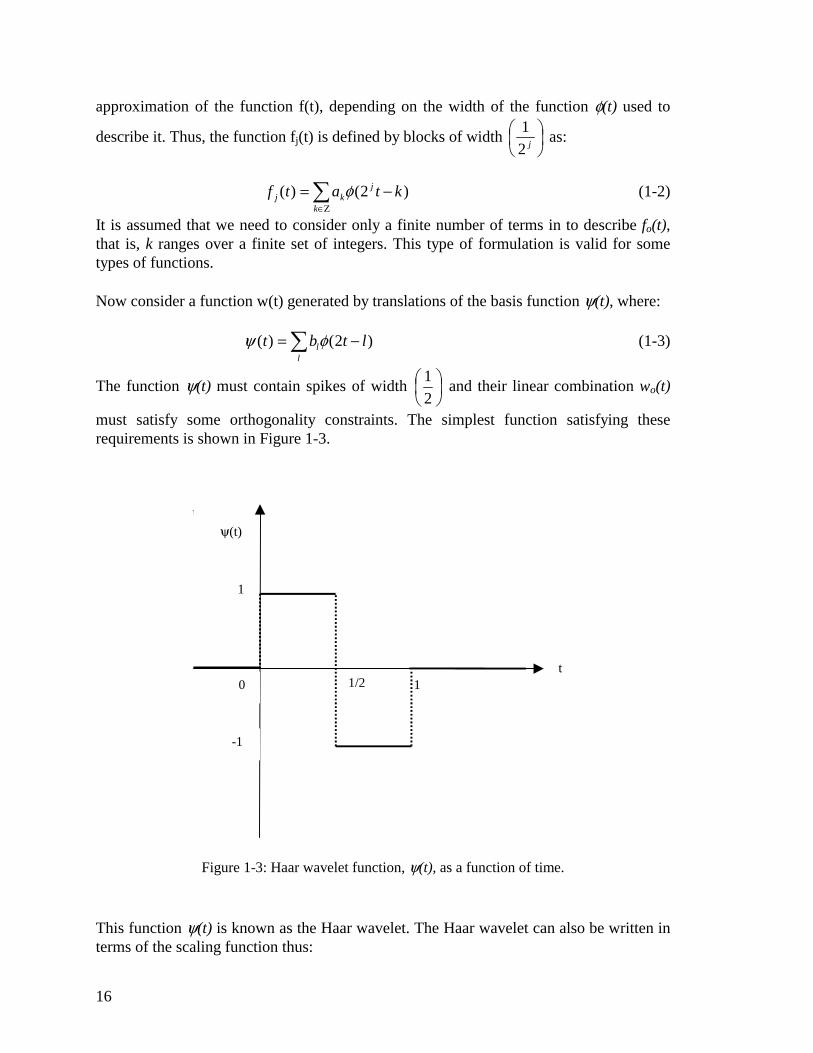
must satisfy some orthogonality constraints. The simplest function satisfying these requirements is shown in Figure 1-3.

ψ(t)ψ(t)

1

0t

-1

1/2 1

ψ(t)

Figure 1-3: Haar wavelet function, ψ(t), as a function of time.

This function ψ(t) is known as the Haar wavelet. The Haar wavelet can also be written in terms of the scaling function thus:

17

)12()2()( −−= ttt φφψ (1-4) For j = 1, f1(t) is the piecewise continuous approximation of f(t) defined by blocks of

thickness

2

1. We would like to express:

)()()( 001 twtftf += (1-5)

where: ℜ∈−= ∑∈

kZk

jkj aktatw K)2()( ψ (1-6)

In this way, the original sampled function f(t) can be successively decomposed in terms of the unique sum:

)()()()()( 0021 tftwtwtwtf jjj ++++= −− KK (1-7)

The process of expressing a function in this form is called Wavelet Decomposition.

Thus, we can express the original function in a form that gives us information about all the frequencies used to describe the function at different resolutions determined by the

width

j2

1of the scaling function. This enables us to choose and modify the function at

the resolution desired, by selectively modifying the corresponding frequency. Thresholding, as explained in this section, is one such process that involves setting low amplitude frequencies to zero in order to smooth out the function.

The wavelet functions and the scaling function can now be combined in order to give back the original function or suitably modified version of the original function. This process is called Wavelet Reconstruction.

It is important to note that for complete decomposition, k is required to be a power of two. Also, the Haar wavelet decomposition requires exactly the same storage as the original sampled signal.

In two dimensions, using the same theory developed for the one-dimensional case, an nxn matrix can be expressed as a corresponding nxn matrix of wavelet coefficients as shown in Figure 1-4. The implementation [Wickerhauser, 1994] is based on the following set of equations for the computation of the coefficients.

Wavelet Decomposition Equations

In two dimensions, Haar wavelet decomposition is carried out using the definition of wavelet coefficients at each successive resolution [Boggess, 2001]. A distribution (image) consisting of nxn grid-blocks (pixels). The scaling coefficient at location p is defined denoted by aj+1(p) and the wavelet coefficient is given by dj+1(p).

18

∑∞

−∞=+ ++=−=

njjjj pahpahnapnhpa )12()1()2()0()()2()(1 (1-8)

where

==

otherwise

nifnh

0

1,02

1)( (1-9)

Substituting these coefficients we obtain:

( ))12()2(2

1)(1 ++=+ papapa jjj (1-10)

or in general, ∑−

=

+

=

12

00 )2(

2

1)(

j

n

j

j

j ipapa (1-11)

the corresponding wavelet coefficients are given by the expression:

∑∞

−∞=+ ++=−=

njjjj pagpagnapngpd )12()1()2()0()()2()(1 (1-12)

where,

=

=−

=−−= −

otherwise

nif

nif

nhng n

0

12

1

02

1

)1()1()( 1 (1-13)

( ))12()2(2

1)(1 ++−=+ papapd jjj (1-14)

Thus it is easy to imagine the scaling coefficient as the normalized arithmetic average of two adjacent data points of the full matrix, located at p and 2p+1. The wavelet coefficient or contrast can be imagined as the arithmetic difference of these two adjacent coefficients.

The number of levels of decompositions possible or number of different resolutions is L:

nL 2ln= (1-15) where n = dimension of square matrix, and a power of 2.

Once the decomposition is complete at all levels, the coefficients can be modified or thresholded as the algorithm requires and overwritten onto the original decomposition.

Wavelet Reconstruction Equations

Wavelet reconstruction is the inverse process of wavelet decomposition. If the inversion is performed without modifying the coefficient in the intermediate thresholding stage, the reconstructed image is identical to the original image. The Haar wavelet reconstruction equations are derived from the decomposition equations:

19

( ))()(2

1)()0()()0()2( 1111 pdpapdgpahpa jjjjj ++++ −=+= (1-16)

( ))()(2

1)()1()()1()12( 11111 pdpapdgpahpa jjjjj +++++ +=+=+ (1-17)

Since the wavelet transform is a linear transform, therefore any wavelet coefficient aj(p) is a linear combination of the original signal a0.

As an example, Equations 1-11 and 1-14 may be used to decompose the gray-scale image of Lenna as shown in Figure 1-4. After wavelet decomposition, the wavelet coefficients corresponding to the pixels are obtained. The matrix at the bottom depicts the different sets of scaling and wavelet coefficients and the as well as the locations of those wavelet coefficients that are required to reproduce the original image to some degree of accuracy.

20

W

d11

d33d32

d31

d23

d21

d12 d13

d22

a

Figure 1-4: Haar Wavelet Decomposition Algorithm applied to the image of Lenna [Lu, 2001].

21

After performing the Haar wavelet transform on an image we obtain the corresponding wavelet transform matrix. This matrix contains wavelet coefficients that can be linearly transformed back to give the original image. However, usually it is only a smaller subset of these frequencies that are required to capture the essential features of the image. The rest of the frequencies with amplitude lower than a set threshold can be set to zero without significantly affecting the reconstructed image. Criteria other than low amplitude can also be used as deciding factor for setting a subset of coefficients to zero. This process will be referred to as ‘thresholding’ in the remainder of this report. Figure 1-5 shows on the left-hand side, areal permeability distributions in millidarcies (ranging from 0-1200md) and on the right hand side the sets of wavelet frequencies that are used to describe the distribution on the left. We can see that as the threshold is increased, the permeability distribution deviates from the original and becomes smoother and smoother in some regions, while keeping the original resolution in other regions. The history obtained by simulation using these distributions, deviates from the reference history. The thresholding is done based on the response to production. This is done by retaining the wavelet coefficients that are required maintain the history match. Production history, for example, watercut data, deviates further and further from the reference data as the threshold is increased as seen in Figure 1-6. It is observed, however, that until a certain threshold, the history is preserved quite well. This leads to the conclusion that some set of wavelet frequencies can be set to zero without significantly changing the history response of the permeability distribution.

22

1024 coefficients

410 coefficients

256 coefficients

Figure 1-5: Areal permeability distributions and corresponding pattern of nonzero wavelet coefficients required to describe the distributions.

23

0

5

0

5

0

5

0

205 coefficients

174 coefficients

113 coefficients

Figure 1-5 continued: Areal permeability distributions and corresponding pattern of nonzero wavelet coefficients required to describe the distributions.

24

93 coefficients

Figure 1-5 continued: Areal permeability distributions and corresponding pattern of nonzero wavelet coefficients required to describe the distributions.

0

0.1

0.2

0.30.4

0.5

0.6

0.7

0 100 200 300 400 500 600

t ime ( d a ys )

Number of constrainingwavelet coefficientsdecreases

1

2

3

4

5

1: original - 1024 coefficients. 2: 265 coefficients. 3: 205 coefficients. 4: 174 coefficients. 5: 113 coefficients.

WC

T

Figure 1-6: Watercut versus time – variation with decrease in number of history-constraining

wavelet coefficients included.

25

1.2.1. Sensitivity Coefficients

Sensitivity coefficients are derivatives of the response variables (pressure and watercut) with respect to the estimated parameters. In wavelet space, these parameters are in the form of wavelet coefficients corresponding to the permeability field. These sensitivity coefficients record the relative impact of a change in a particular parameter on the history response of the field. Thus the sensitivity coefficients corresponding to the history of the reservoir quantify coefficient by coefficient how much the history would change if that coefficient is changed. The higher the sensitivity coefficient corresponding to a particular frequency the more the history will deviate from the original if the corresponding wavelet coefficient of the permeability distribution was changed.

The concept of sensitivity coefficients has introduced in 1974 by Carter, Pierce, Kemp and Williams. This concept was further developed in the 1970s and early 1980s [Chen, Gavalas, Seinfeld and Wasserman 1973]

Chu, Reynolds and Oliver, [1995] used a modified technique for the calculation of sensitivity coefficients that was efficient and enabled the application of the Gauss-Newton algorithm for parameter estimation and the geophysical inverse theory to include a priori information. An alternative procedure, called the gradient simulator, was developed by Anterion, Eymard & Karcher to compute sensitivity coefficients. Literature shows several applications of these methods one of which is in a work by Bissel [1996].

1.2.2. Wavelet Coefficients Constraining History Match

A Haar wavelet transform of the history matched permeability field yields a set of wavelet coefficients. As shown by Lu [2001], there is a subset of these wavelet coefficients that have a high sensitivity to the history data. That is, changing the value of the members of this set of wavelet coefficients leads to a sizeable change in the production response of the corresponding permeability field. This ‘sensitivity’ to production data is quantified by the sensitivity matrix in wavelet space that consists of sensitivity coefficients. The members of the sensitivity matrix are positive, bounded values corresponding to each wavelet coefficient of the permeability field. On the basis of this sensitivity matrix, the wavelet coefficients of the permeability field can be ranked in order of importance to history match, the higher rank coefficients corresponding to high sensitivity values. If we start thresholding the lower ranked coefficients (setting them to zero), we see that the history match of the inverted permeability field starts getting worse. Thus, a tolerance level can be set that defines a threshold that reproduces the history data corresponding to the field reasonably. Setting some of the coefficients to zero has the effect of smoothing the resulting permeability field nonuniformly. Thus, out of the set of all wavelet coefficients of the permeability field only the nonzero coefficients are actually used to obtain this smoothed permeability field that still has the same history as the original, within the limits of a predetermined tolerance. This set is the set of wavelet coefficients that is said to constrain the history match.

26

1.2.3. Wavelet Coefficients Constraining Geostatistical Parameters

It is conjectured that a set of wavelet coefficients can be found that are sensitive to the geostatistical parameter chosen to describe the reservoir. This set need not be unique and it is possible that it might partially or wholly overlap with the set of history-constraining wavelet coefficients. The geostatistical parameter used in this study was the variogram of the permeability distribution, based on prior knowledge of the geology of the region.

The variogram, [Deutsch and Journel, 1998], is a useful measure of two-point geostatistics and is defined as the variance of the increment )]()([ huZuZ +− where

)(uZ is a generic random variable (in our case the permeability value) at location u.

For stationary random functions,

)}()({)(2 huZuZVarh +−=γ (1-18)

)()0()( hCCh −=γ (1-19)

with: C(h) being the stationary covariance, and C(0) = Var{Z(u)} being the stationary variance.

The variogram is used as a geostatistical tool for modeling spatial variability. A typical isotropic variogram for permeabilities is shown in Figure 1-7. The variogram plots the magnitude of the variogram as a function of distance of separation between two locations (u) and (u+h). The variogram is a means of quantifying the spatial distribution of random functions in Gaussian fields.

27

NuggetEffect

Range

Figure 1-7: Isotropic normal score variogram for two dimensional permeability distribution.

The variogram considered in the objective function of the optimization routine can be an isotropic variogram or an anisotropic variogram. This parameter works well for Gaussian fields that do not have features like channels or faults. The variogram as such can not be used directly to characterize a permeability field that has such features. On the other hand for Gaussian fields, the variogram gives a good indication of the spatial variability and distribution of the permeability values in the grid on small as well as larger scales of the order of the field. Thus we see that the variogram prescribes spatial variability at different resolutions. There is a set of wavelet coefficients that determine the variogram of a permeability distribution. In this study it was found, in the various cases considered, that this set is not necessarily a unique one.

1.2.4. Decoupling of Wavelet Coefficients Constraining History Match and the Geostatistical Parameter

The algorithm implicitly assumes that once the wavelet coefficients constraining the production history of the permeability distribution are fixed, it is possible to modify the ‘free’ coefficients in order to match the variogram. In other words, the integration of geostatistical data into the existing model is dependent on being able to find this set of variogram-constraining wavelet coefficients, among the ‘free’ coefficients. There are three possible scenarios regarding the nature of the relationship of the two sets of constraining wavelet coefficients, as can be seen in Figure 1-8. Case I describes the scenario that the sets overlap to some extent. If this were the case and the history constraining wavelet coefficients were fixed, a subset of the variogram-constraining

28

coefficients would be fixed at the same time. As such we might not be able to match the variogram accurately, depending on the degree of overlap. Case II describes the situation in which the two sets are perfectly disjoint. In this case, it would be possible to match the variogram better, by using the full set of constraining coefficients. Case III is one in which the set of variogram-constraining coefficients are a subset of the history constraining wavelet coefficients. As such, once the set of history-constraining wavelet coefficients are fixed, the variogram is fixed as well and would not possible to modify the coefficients on order to get a variogram match.

Constrained by History Match

Free to be constrained by Geological Information

Case 1 Case 2

Case 3

Figure 1-8: Three possible scenarios for the relation between sets of wavelet coefficients constrained by history match and geostatistical information.

The integration of geostatistical data would be most effective for reservoirs in which the sets of wavelet coefficients were perfectly disjoint (Case II) or if they overlap only to a small degree (Case I). It is thought that most reservoirs would have sets of wavelet coefficients that resembled case I.

29

Chapter 2

2. Data Integration Methodology and Implementation

The data integration procedure, using wavelet decomposition and separation, consists of three main parts:

1. The history matching code that generates a history-matched permeability distribution;

2. The optimization routine that integrates variogram information;

3. The Haar wavelet toolbox that allows for manipulation of wavelet coefficients.

The flow simulator yields a permeability distribution that matches the reference history and generates a set of sensitivity coefficients in wavelet space. This algorithm [Lu 2001] uses wavelet-based parameter estimation in order to match history. The Haar wavelet transform of the permeability field is performed and is followed by thresholding based on the magnitude of the wavelet sensitivities. This enables a reduction in the number of parameters that need to be determined in order to match the history. As a result, instead of perturbing individual permeability values in the grid blocks, history matching is done by varying a smaller subset of wavelet coefficients. Hence, the wavelet algorithm is much more efficient than conventional algorithms that are based on varying individual permeability values in grid blocks. The wavelet algorithm generates a permeability distribution that matches the given reference history. The algorithm also determines the sensitivity matrix of the permeability distribution in wavelet space. This sensitivity matrix consists of coefficients that quantify the ‘sensitivity’ (see Section 1.2.1) of the corresponding wavelet coefficients of the permeability distribution to the production response. If the magnitude of the sensitivity coefficient is high, it implies that the corresponding wavelet coefficient of the permeability distribution is ‘important’ for the history match. This means that that particular coefficient needs to be retained in order for the distribution obtained by wavelet inversion to match the reference history. If the magnitude of the sensitivity coefficient is low, the corresponding wavelet coefficient of the permeability distribution can be set to zero or to any other bounded value without significantly affecting the history match. The threshold used to decide whether a permeability distribution wavelet coefficient is determined internally within the history matching code based the tolerance set on the history match. Only the permeability distribution wavelet coefficients with a sensitivity to history that is higher than the threshold are perturbed to obtain a history match. The distribution of this set of frequencies is referred to as the ‘mask’. The masked wavelet coefficients constrain the production response and are fixed at this stage. These particular coefficients are not

30

changed subsequently in the course of the integration of geostatistical information. This is equivalent to ‘fixing’ the history response of the permeability field.

The second part is the optimization routine that integrates geostatistical information into the history-matched permeability distribution. This routine perturbs the ‘free’ or ‘unmasked’ wavelet coefficients of the permeability distribution that are not already constrained by the history-matching algorithm in order to minimize an objective function. The optimization routine employed is Simulated Annealing [Gill and Murray, 1981] and the objective function used is the norm of the difference between the variogram of the history-matched distribution and the reference variogram. The algorithm perturbs a ‘free’ wavelet coefficient and then applies a wavelet back-transform to obtain the corresponding permeability distribution. The procedure then calls the geostatistical software GSLIB [Deutsch and Journel, 1998] and calculates the objective function. The perturbation is accepted or rejected based on the change in magnitude of the objective function. Once the objective function is sufficiently minimized, or the maximum number of iterations is reached, the simulated annealing algorithm is terminated. The final permeability distribution reproduces the variogram that describes the spatial distribution of permeability values in the field. Importantly, because the wavelet coefficients constraining the history matched were not changed, the history match is also retained.

The third piece that fits into the algorithm is the Haar wavelet toolbox that was written in Matlab. This toolbox has routines for wavelet transform, inverse transform, thresholding and coefficient manipulation. The wavelet toolbox is used to determine and manipulate the history-constraining coefficients. Also, at each iteration of the simulated annealing algorithm in wavelet space, the inverse transform is performed in order to calculate the objective function in real space. Since the wavelet operations are linear operations, these transformations back and forth from wavelet space to real space are very fast (see Section 1.2 for decomposition-reconstruction formulae).

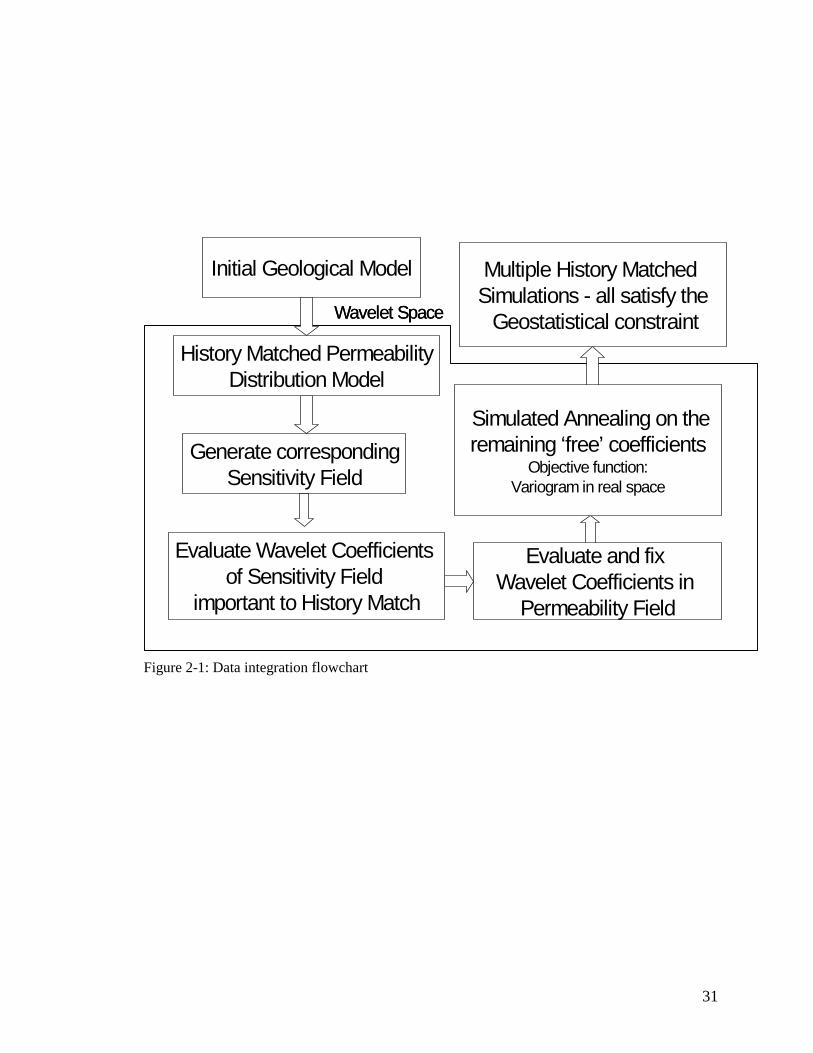
The algorithm is described in the form of a flowchart in Figure 2-1. Figure 2-2 shows the workflow for the algorithm as applied to a reference two-dimensional multiphase flow reservoir model.

31

Evaluate Wavelet Coefficients of Sensitivity Field

important to History Match

Initial Geological Model

History Matched Permeability Distribution Model

Evaluate and fix Wavelet Coefficients in

Permeability Field

Generate corresponding Sensitivity Field

Wavelet SpaceWavelet Space

Multiple History Matched Simulations - all satisfy the

Geostatistical constraint

Simulated Annealing on the remaining ‘free’ coefficients

Objective function:Variogram in real space

Figure 2-1: Data integration flowchart

32

History-Matched Permeability Distribution

History-Matched and GeologicallyConstrained Permeability Distribution

Wavelet Mask

Wavelet Space

Sensitivity Matrix History-Matched Permeability DistributionHistory-Matched Permeability Distribution

History-Matched and GeologicallyConstrained Permeability Distribution

Wavelet MaskWavelet Mask

Wavelet SpaceWavelet Space

Sensitivity MatrixSensitivity Matrix

Figure 2-2: Data integration workflow using a two-dimensional permeability distribution model.

33

Chapter 3

3. Sensitivity Analysis

3.1. Amount of Useful Production History Information

The ‘amount’ of history data is described in terms of:

1. The number and distribution of wells from which the data are obtained. The greater the number of wells and the wider their distribution in the reservoir, the more the permeability distribution is constrained by the history data.

2. Water breakthrough at a well. If the history data contains water breakthrough information at a well, they give us more information about the permeabilities in the neighborhood of the well.

It was observed that the ‘more’ the constraining history information available for the reservoir, the greater is the number wavelet coefficients retained in the mask. As a result a fewer number of coefficients are available as parameters for the integration of geostatistical information. To verify this hypothesis, a test case was chosen and the effect on the wavelet mask of gradually increasing the amount of history data was observed. The test case was a permeability distribution with three wells, one water-injection well and two production wells as shown in Figure 3-1 and Figure 3-2. As more and more data were used to constrain the permeability distribution, two effects were observed. Firstly, the wavelet mask was found to contain more nonzero entries whose spread depended on the position of the waterfront. Secondly the sensitivity coefficients increased in magnitude. However, after a certain critical limit of production data inclusion, the wavelet mask did not change. This implies that there exists a certain critical amount of production data such that additional data does not significantly change the nature of the wavelet mask as it only has the affect of increasing the magnitude of the already included sensitivities. Once this critical production data limit is reached, no more history data is necessary to determine the wavelet mask for the field barring the addition of infill wells or water breakthrough in an existing well.

34

Isha 3: Reference PermeabilityDistribution

5 10 15 20 25 30

5

10

15

20

25

30

0

200

400

600

800

1000

1200

1400

1600

Case I

4600

4700

4800

4900

5000

5100

5200

5300

5400

5500

0 200 400 600

Time (days)

rsur

Psa)

0

0.1

0.2

0.3

0.4

0.5

0.6

0.7

0.8

0.9

1

WCT

Injector Pressure

Producer 1 Pressure

Producer 1 WCT

Producer 2 Pressure

Producer 2 WCT

Figure 3-1: Reference permeability distribution with Case I production history and wavelet mask.

35

Case II

4600

4800

5000

5200

5400

5600

5800

0 200 400 600

Time (days)

Pre

ssur

e (p

sia)

0

0.1

0.2

0.3

0.4

0.5

0.6

0.7

0.8

WC

T

Ref Pressure Producer 1

Ref Pressure Injector 1(3,3)


Ref WCT Producer 1

Ref WCT Producer 2

0 5 10 15 20 25 30

0

5

10

15

20

25

30

Case III

0

1000

2000

3000

4000

5000

6000

7000

0 200 400 600

Time (days)

Pre

ssu

re (p

sia)

0

0.1

0.2

0.3

0.4

0.5

0.6

0.7

0.8

0.9

WC

T

Injector Pressure

Producer 1 Pressure

Producer 2 Pressure

Producer 1 WCT

Producer 2 WCT

0 5 10 15 20 25 30

0

5

10

15

20

25

30

Figure 3-2: Case II and III: production history and wavelet mask

36

3.2. Tolerance for History Match and Geostatistical Constraint

In order to retain history data, as explained in the section on thresholding, Section 1.2, the number of wavelet coefficients retained to match the history depends on what the desired accuracy is for the history match. Depending on how low or high one sets the tolerance to history match, the better or worse will be the reproduction of history and the greater number of wavelet coefficients will be free to match the variogram with. In the case that we are unsure of the history data, or if it is known to be erroneous or inaccurate, the tolerance to history match can be relaxed. As a result a higher percentage of wavelet coefficients will be available to us to obtain a more exact variogram match. Thus as seen in Figure 3-3 as the tolerance to history is successively tightened from Case I to Case III, the size of the set of history constraining wavelet coefficients increases and the size of the set of wavelet coefficients free to constrain the variogram increases. The relative sizes of the sets of coefficients can be fixed depending on the certainty of the data and the requirements of the problem.

Wavelet Coefficients constrainingthe production history

Wavelet Coefficients constrainingvariogram

Case I: High Tolerance tohistory match

Case III: Low Tolerance tohistory match

Case II

Figure 3-3: Effect on sets of wavelet coefficients of greater tolerance to production data.

37

3.3. Traversal Techniques

The variogram is incorporated into the reservoir model by means of a simulated annealing algorithm that perturbs wavelet coefficients sequentially in order to minimize a variogram-based objective function in real space. For this study, a number of different traversal techniques were employed within the simulated annealing algorithm. It was found that the resulting permeability distribution in almost all the cases matched the production history as well as the variogram. Even so, the results looked significantly different depending on the order in which the sets of wavelet coefficients were perturbed.

As seen in Section 1.2 the wavelet coefficients at a certain level are related to the contrasts of the image at a particular resolution. It was found that an adequate match to the variogram can be obtained by modifying the wavelet coefficients corresponding to only one direction – either horizontal, vertical or diagonal. Depending on the direction of contrasts perturbed, the results showed greater continuity in the other two orientations. In the same way, by selectively varying wavelet coefficients at different resolutions, we get a set of different results, and yet all reproduce the history as well as the isotropic variogram.

In Figure 3-4, Cases I and V were generated by modifying the vertical and diagonal contrasts at different resolutions. Cases I through IV were generated by modifying only the horizontal contrast. Case VI was generated by varying the diagonal contrasts at all resolutions. Figure 3-5 shows the variograms for some of the cases. It is important to note that the variogram for Case VI shows a very different nugget effect than all the other cases, including the reference. This can also be seen from Figure 3-4 (VI) that shows an unrealistically high degree of heterogeneity due to the particular selection of traversal technique. As a result of the choice of wavelet coefficients and the order of the traversal, a lot of heterogeneity is added to the model at the fine scale, and as such the nugget effect is abnormally high. From these observations, we can conclude that the order of traversal in the Simulated Annealing algorithm affects the appearance of the final permeability distribution result.

It is important to note that, not all of the free wavelet coefficients contribute to the reproduction of the variogram as illustrated in Figure 3-6. There is still a set of remaining ‘free’ coefficients that are free to be perturbed without modifying the history match or the variogram. This set of wavelet coefficients can be varied to include reservoir information from a different source. This conclusion is supported by Figure 3-7 that shows the distribution of history- and variogram- constraining wavelet coefficients for Reservoir II (see Section 4.2.1). Figure 3-7 shows three distinct sets of wavelet coefficients. The history-constraining wavelet coefficients (320 in number) are determined during the history-matching process and are then fixed. The remaining coefficients are then varied to obtain a match for the variogram. It is observed that only a subset (302 in number) of these ‘free’ coefficients are actually changed significantly to obtain the variogram. This set is observed to be nonunique for all the cases studied. The unperturbed wavelet coefficients are shown as white spaces. This set of wavelet coefficients are free to be constrained by some other parameter.

38

Moreover, from Case VI we see that in order to obtain a realistic permeability distribution, it is important to reproduce the nugget effect well. To make sure that the nugget effect is accurate, there might be a need to give more weight to the part of the objective function dependent on the nugget effect.

Case VICase V

Case IVCase III

Case IICase I

Case VICase V

Case IVCase III

Case II

Case VICase V

Case IVCase III

Case IICase I

Figure 3-4: Different permeability distributions obtained using different traversal techniques for

in the variogram integration routine.

39

Figure 3-5: Variograms corresponding to different permeability distributions as shown in Fig. 3-

4.

40

Constrained by History Match

Free to be constrained by Geological Information

Case 1

Independent of both History and Variogram=> Constrained by some other parameter

Figure 3-6: Relationship between sets of wavelet coefficients as observed in test cases.

Figure 3-7: Nonzero pattern for sets of constraining wavelet coefficients

41

Chapter 4

4. Application to Synthetic Reservoirs

In Chapter 2 the methodology and implementation of the wavelet algorithm was described using some test cases of reservoir models. Chapter 3 explored sensitivity and tolerance issues related to the algorithm. In this chapter a number of different multiphase, Gaussian, permeability field examples are used, to test the working of the wavelet based data integration methodology. All the cases described here are based on reservoirs with a 32x32 mesh of gridded permeabilities. The objective function was reduced by up to two orders of magnitude and the algorithm converged within the stipulated maximum number of iterations.

4.1. Reservoir I – 3 wells, multiphase

An areal Gaussian permeability field, as shown in Figure 4-1, was chosen as the reference case. The field history was defined by multiphase production data from four wells, one injector and two producers. The isotropic variogram corresponding to the permeability field is plotted in Figure 4-1. The well locations were chosen so that the history data would provide information over a large fraction of the area of the field. This is reflected in the wavelet mask (Figure 4-2), that shows that a large fraction (up to 40%) of the wavelet coefficients were required to constrain the production history of the field. Figure 4-2 also shows the permeability field as described by only the history-constraining wavelet coefficients that was used as the starting point for the integration of geostatistical information. The simulated annealing routine for variogram incorporation was applied to this starting distribution in order to obtain the multiple history-matched, geostatistically-constrained permeability distributions, out of which six are depicted in Figure 4-3.

In order to check the claim that the production history is indeed retained and that the variogram is satisfied, the pressure and watercut history and well as the variograms of these results were plotted along with the corresponding plots of the reference field (Figure 4-4 and Figure 4-5). It was found that the results exhibited a good visual match to the data corresponding to reference data.

This initial test shows that the algorithm does indeed generate a converged result in under one hour of CPU time. This example also shows, that even when the history data are extensive, starting from a different random seed a number of history-matched and variogram constrained permeability models can be generated.

42

0 5 10 15 20 25 30

0

5

10

15

20

25

30

Injector

Figure 4-1: Reservoir I: Permeability field with distribution of wells and variogram.

43

0 5 10 15 20 25 30

0

5

10

15

20

25

30

Permeability Distribution: Starting Point

5 10 15 20 25 30

5

10

15

20

25

30

0

200

400

600

800

1000

1200

Figure 4-2: Reservoir I: Nonzero pattern for production history constraining wavelet coefficients

and the corresponding thresholded permeability distribution.

44

Permeability Distribution: Result 1

5 10 15 20 25 30

5

10

15

20

25

30

0

200

400

600

800

1000

1200


5 10 15 20 25 30

5

10

15

20

25

30

0

200

400

600

800

1000

1200


5 10 15 20 25 30

5

10

15

20

25

30

0

200

400

600

800

1000

1200


5 10 15 20 25 30

5

10

15

20

25

30

0

200

400

600

800

1000

1200


5 10 15 20 25 30

5

10

15

20

25

30

0

200

400

600

800

1000

1200


5 10 15 20 25 30

5

10

15

20

25

30

0

200

400

600

800

1000

1200

Result 3

Result 4

Result 5 Result 6

Result 3

Result 2Result 1

Figure 4-3: Reservoir I: Permeability distributions obtained using data integration algorithm.

45

Pressure History - Well # 1

5000

5500

6000

6500

7000

7500

8000

0 100 200 300 400 500

time (days)

Pre

ssu

re (

un

its)


2000

2500

3000

3500

4000

4500

5000

0 100 200 300 400 500

time

Pre

ssu

re (

un

its)


1000

1500

2000

2500

3000

3500

4000

4500

5000

0 100 200 300 400 500

time (days)

Pre

ssu

re

WCT History - Well # 2

0

0.1

0.2

0.3

0.4

0.5

0.6

0.7

0.8

0.9

1

0 100 200 300 400 500

time (days)

WC

T

WCT History: Well # 3

0

0.1

0.2

0.3

0.4

0.5

0.6

0.7

0.8

0 100 200 300 400 500

time (days)

WC

T

original

pert1

pert3

pert5

pert7

D2

D3

halfconvergedThresholded

Pressure History: Well # 4

1500

2000

2500

3000

3500

4000

4500

5000

0 100 200 300 400 500

time (days)

Pre

ssu

re (

un

its)

Figure 4-4: Reservoir I: Pressure and watercut history – reference and results.

46

Starting Variogram

Reference Variogram

Figure 4-5: Reservoir I: Variogram match – reference, starting point and final results.

47

4.2. Fields with Limited History Data

A number of different reservoir models were developed to test the data integration algorithm. The initial cases were chosen to have fewer wells so that the set of wavelet coefficients constraining the history of the distribution would be limited. In other words, the fields were chosen such that the production history would not be overly constraining.

4.2.1. Reservoir II – 2 wells, multiphase

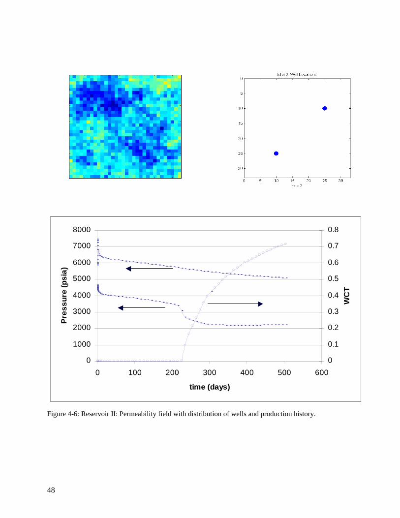
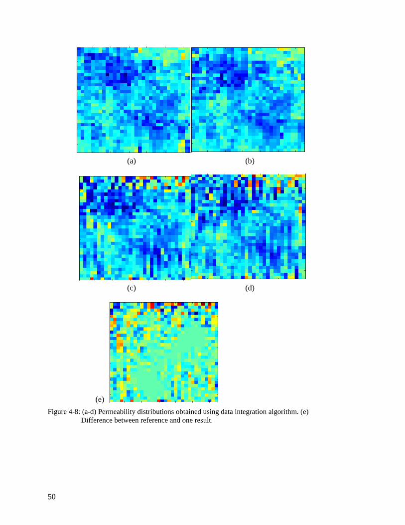
This reservoir model was chosen to have a permeability distribution as shown in Figure 4-6. The sources of production history are two wells, one injector and one producer as shown in Figure 4-6. The reference history is in the form of pressure and watercut information with respect to time for the two well. Figure 4-7 shows the distribution of history-constraining wavelet coefficients – about 30% of the wavelet coefficients are retained for the history match. As expected, this is a lower percentage than was observed in Reservoir I, since we have only two wells as compared to four in the previous case. We can see a diagonal stripe corresponding to the path between the wells in each set of the history-constraining wavelet coefficients in Figure 4-7. This shows that the production history data obtained from this reservoir is dependent mostly on the average permeabilities that lie in the path of the waterfront from the injection well to the production well. Figure 4-7 also shows the permeability field description using only this set of history-constraining wavelet coefficients that are held constant. This acts as the starting point for the geostatistical data integration algorithm. After the optimization routine that modifies the field to match the reference variogram we obtain a history- and variogram- matched permeability model. This optimization routine can be repeated with a different random seed in order to obtain distinct permeability model results as seen in Figure 4-8. The corresponding variograms and production histories, along with those of the reference are plotted in Figure 4-9. We see that the results have production histories and variograms that closely match that of the reference.

48

0

1000

2000

3000

4000

5000

6000

7000

8000

0 100 200 300 400 500 600

time (days)

Pre

ssur

e (p

sia)

0

0.1

0.2

0.3

0.4

0.5

0.6

0.7

0.8

WC

T

0

1000

2000

3000

4000

5000

6000

7000

8000

0 100 200 300 400 500 600

time (days)

Pre

ssur

e (p

sia)

0

0.1

0.2

0.3

0.4

0.5

0.6

0.7

0.8

WC

T

Figure 4-6: Reservoir II: Permeability field with distribution of wells and production history.

49

Figure 4-7: Wavelet mask and thresholded permeability distribution obtained by retaining

coefficients constraining production history.

50

(a) (b)

(c) (d)

(e)

Figure 4-8: (a-d) Permeability distributions obtained using data integration algorithm. (e) Difference between reference and one result.

51

0

1000

2000

3000

4000

5000

6000

7000

8000

0 200 400 600

time (days)

Pre

ssur

e (p

sia)

0

0.1

0.2

0.3

0.4

0.5

0.6

0.7

0.8

WC

T

result 1

reference

Reference

result1

result 5

result 2

result2

result 3

result 3

result 5

Thresholded

Thresholded

result 5

Reference

Figure 4-9: Reservoir II: Production history and isotropic variogram – reference and results.

52

4.3. Field with History data in a small region of the reservoir

It is likely that in the initial stages of the development of a reservoir production history might be available from wells developed in a small region of the field. In order to forecast the production from infill wells drilled subsequently in a different part of the reservoir, a full field reservoir model is required. The existing wells only provide information about a region of the reservoir that is local to the wells. Thus there is a need to make maximum use of the limited information provided by the existing wells and at the same time, utilize geostatistical data in order to generate reservoir models stochastically.

4.3.1. Reservoir IV – 3 wells

This test case is a synthetic Gaussian permeability field, with variogram and production history from three wells (one injector and two producers) as shown in Figure 4-10. The production data is limited to a small part of the reservoir, and this is reflected in the wavelet mask as well as the history-constrained permeability distribution in Figure 4-11. We see that less than 20% of the wavelet coefficients are retained in order to match the production history and the remaining are free to be constrained by other parameters like the variogram. This reflects the actual uncertainty associated with a reservoir with only very limited production data available.

Using the data integration algorithm developed in this work, this limited data can be integrated efficiently with available geostatistical data in order to generate a set of equiprobable permeability models as shown in Figure 4-12. The history and variogram data, corresponding to these results, are plotted together with the reference data in Figure 4-13 and Figure 4-14. We can see that even though the permeability distributions do not look alike, the production history and variogram for all the results are in good agreement with the reference data.

53

Reservoir Isha IVIsotropic Vari ogram

I s h a 3 : R e f e re n ce P e rm e a b ilit yD is t r ib u ti o n

5 1 0 1 5 2 0 2 5 3 0

5

1 0

1 5

2 0

2 5

3 0

0

2 0 0

4 0 0

6 0 0

8 0 0

1 0 00

1 2 00

1 4 00

1 6 00

γ

4000

4200

4400

4600

4800

5000

5200

5400

5600

5800

0 200 400 600

Time (days)

Pre

ssu

re (

psi

a)

0

0.1

0.2

0.3

0.4

0.5

0.6

0.7

0.8W

CT

Ref PressureProducer 1

Ref Pressure Injector1 (3,3)

Ref PressureProducer 2

Ref WCT Producer 1

Ref WCT Producer 2

Figure 4-10: Reservoir IV: Permeability distribution, variogram and reference production history.

54

0 5 10 15 20 25 30

0

5

10

15

20

25

30

Figure 4-11: Reservoir IV - Wavelet mask and thresholded permeability distribution obtained by

retaining coefficients constraining production history.

55

Result 2 Result 2

Result 4 Result 3

Result 1

Result 7 Result 8

Result 6 Result 5

Figure 4-12: Permeability distributions obtained using data integration algorithm

56

4550

4750

4950

5150

5350

5550

5750

0 100 200 300 400 500 600

Time (days)

Pre

ssu

re (

psi

a)


Ref Pressure Injector 1 (3,3)


Thresholded Injector Pressure

Thresholded Producer 1 Pressure


Result 1 - Injector Pr

Result 1 - Producer 1 Pr









Result 4 - Producer 1 Pressure



Result 5 - Injector 1 Pr





Isha 3: History Match - Reference and Results

0

0.1

0.2

0.3

0.4

0.5

0.6

0.7

0.8

0 100 200 300 400 500 600

time (days)

WC

T

Ref WCT Producer 1

Ref WCT Producer 2

Thresholded Producer 1 WCT


Result 1 - Producer 1 WCT












Isha IV

4550

4750

4950

5150

5350

5550

5750

0 100 200 300 400 500 600

Time (days)

Pre

ssu

re (

psi

a)


Ref Pressure Injector 1 (3,3)


Thresholded Injector Pressure













Result 4 - Producer 1 Pressure



Result 5 - Injector 1 Pr





Isha 3: History Match - Reference and Results

0

0.1

0.2

0.3

0.4

0.5

0.6

0.7

0.8

0 100 200 300 400 500 600

time (days)

WC

T

Ref WCT Producer 1

Ref WCT Producer 2















Isha IV

Figure 4-13: Reservoir IV – Production history, pressure and watercut for reference and results.

57

starting variogram

reference variogram

starting variogram

reference variogram

Figure 4-14: Reservoir IV –Isotropic variogram reference, starting point and Result1 (from

Figure 4-12).

58

Chapter 5

5. Observations and Discussion

It is of great importance to include geological data into reservoir models in order to ensure realistic models that yield better production forecasts. Conventional history matching techniques, as shown in Figure 5-1 [Wang, 2001], might lead to unrealistic reservoirs models that do match the production history but fail to predict future production.

Reference History-matched using Streamlin

Figure 5-1: (a) Reference permeability field (b) History matched model using streamline

algorithm shows streamline artifacts from Wang [2001].

This problem, of obtaining geologically unrealistic history-matched permeability models, can be resolved by the inclusion of geostatistical data descriptive of the nature of the distribution, in order to yield a better reservoir model. Herein lies the relevance of this study of production and geostatistical data integration.

Some key observations made during the course of the study demonstrate, with the help of synthetic reservoirs, that there exist a number of geologically consistent permeability distribution models, all of which satisfy the available production information.

5.1. Decoupling of Sets of Wavelet Coefficients.

The most important result of this algorithm is the observation that the sets of history and wavelet constraining coefficients can be decoupled. Two sets of wavelet coefficients can be determined, one that constrains the history of the reservoir and the second that

59

constrains a geostatistical parameter, in this case, the variogram. From among the scenarios described in Figure 1-8, Case I was the one that was found to be true in all the models studied. In Case I, the sets of history and variogram constraining wavelet coefficients overlap to a small degree but are largely independent. In particular, after fixing the history- and variogram- constraining coefficients of the reservoir, there is still a remaining set of ‘free’ coefficients that is non-unique across the different results, as described in Figure 3-6. An important implication of the existence of this scenario is that the integration of production and geostatistical data can be done sequentially by perturbing only one set of wavelet coefficients at a time. History matching, being a slow and expensive process, is performed once and the history-sensitive wavelet coefficients fixed. The variogram is then incorporated using an iterative wavelet optimization routine. This optimization routine, being wavelet-based, is much faster and more efficient due to the linear nature of wavelet transforms and due to the reduction of optimization parameters. As such, the algorithm developed in this study generates history-matched, geologically consistent permeability results up to 25 times faster than current algorithms developed to give the same results. The set of ‘free’ coefficients may subsequently be used in order to integrate some other parameter or information into the reservoir model.

5.2. Wide Application and Modular Design of Algorithm

The algorithm developed in this study uses three modules, history matching, geostatistical parameter estimation and the Haar wavelet toolbox. Each of these three modules is called independently from the main code. As such, the main data integration code is independent of the working of each component. The advantage of this particular design of the code is that the existing modules can be replaced by other modules that generate the same type of output, given the same set of input arguments depending on the requirements of the problem. For example, the history-matching module can be replaced by any equivalent commercial program. The geostatistical parameter can be changed from the variogram to the correlation length, the histogram or even to multipoint geostatistics. The Haar wavelet toolbox can be replaced by higher order Daubechies wavelets or even wavelets in higher dimensions.

5.3. Potential Applications

The wavelet algorithm developed in this study enables the efficient integration of geological interpretations of the field in history-matched models for better reservoir description. At the same time, it yields multiple equiprobable reservoirs descriptions, giving a probabilistic solution to the problem. This is called stochastic modeling of reservoir and all the solutions are history-matched and geostatistically constrained. The fact that this algorithm yields multiple solutions is more representative of the inherent uncertainty due to lack of sufficient information to determine the permeability distribution deterministically.

Not only does the algorithm include uncertainty based on our information about the reservoir, it also enables the propagation of this uncertainty in the prediction runs for

60

history-matched models. In the case of the development of infill wells in oil-fields with sparse history information, using a number of different models for prediction runs is useful in providing a bound on the future production and reservoir response. This information, in turn helps in making better informed reservoir management and economic decisions for the reservoir.

61

Chapter 6

6. Scope for Further Study

6.1. Integration of Multipoint Geostatistics

The variogram is a useful tool in describing the nature of Gaussian permeability fields, of the kind that were used in this study. However, for permeability fields with channels or other complex geological structures or forms, reproduction of the variogram fails to ensure the reproduction of these complex shapes in the reservoir. The variogram, therefore, cannot be considered to be an adequate tool to describe the geostatistical properties of the field. Consequently, it should not be used as the parameter in the objective function for the integration of geostatistical information into the reservoir model in such cases.

For reservoirs with such complicated geological structures, the variogram should be replaced by parameters corresponding to multipoint geostatistics. This can be incorporated into the algorithm easily by replacing the current variogram-dependent objective function by one that relies in multipoint geostatistics, for example the training image.

6.2. Integration of Data from Other Sources

As seen in Figure 3-6 after the integration of production history and geostatistical data, into the reservoir model, there still exists a set of wavelet coefficients that are not fixed or dependent on either of these two types of data. It is conjectured that these wavelet coefficients can be varied in order to integrate a third source of reservoir data, without affecting the history or the variogram match.

6.3. Weighting of Tolerance Based on Degree of Trust in Source of Data

As discussed in Section 3.2, varying the tolerance on the history data changes the size of the set of wavelet coefficients constraining production history. The higher the tolerance, the greater is the set of wavelet coefficients free to be constrained by the variogram. Now, in case it is known that the production data is inaccurate to some degree, it is useful to increase the tolerance to history data (by increasing the threshold) and retain more coefficients for the variogram match. Thus, we can define a weighting function that varies according to the certainty of a particular data type. The more certain we are about the accuracy of a particular source of data, the more weight can be assigned to it as compared to data from other sources. This weight is related directly to the tolerance set for that

62

particular data, which in turn controls the size of the corresponding set of constraining wavelet coefficients.

6.4. Extension to Three Dimensions

As discussed in Section 5.2, the algorithm is modular in design. As a result, it can be used to solve three-dimensional reservoir problems by replacing the two-dimensional Haar wavelet toolbox module by wavelet descriptions in three dimensions. This would require the development and implementation of wavelet transform operations like decomposition, thresholding and reconstruction in three dimensions. The history-matching algorithm would then be run on the three-dimensional permeability distribution to yield three-dimensional sensitivity coefficient matrices. The geostatistical parameter used, that is, the variogram can be generalized to a set of anisotropic horizontal and vertical variograms.

6.5. Time Variation of Sensitivity Coefficients

An important question left open by this study is the effect of the variation of the sensitivity coefficients with time. It is possible that some wavelet coefficients are ‘important’ to history match for some part of the production history duration while others become more important at a later time. One example of this type of situation occurring is in a multiphase reservoir when a well has water breaking through at a later time than the other wells in the reservoir. The sensitivity information is taken as a weighted combination of sensitivities over the entire period of production history. Consider a well that breaks through at a later time in comparison to the total duration of available production history. As a consequence, the sensitivity coefficients corresponding to the history of that well become active at a later stage and their effect is reduced by averaging over the entire time duration of production. Having lower sensitivity coefficients has the effect of retaining fewer wavelet coefficients that constrain the history of that particular well and as a result the reproduction of history is less accurate than that for the other wells. This effect can be observed in illustrated Reservoir I described in Section 4.1. As can be seen in the bottom right plot of watercut versus time for well number 3 in Figure 4-4, water breakthrough occurs in this well at around 350 days as compared to the available production history of 500 days. The sensitivity coefficients are therefore active for only about 30% of the total production time. This has the effect of reducing the accuracy of the history match in this particular well as can be seen from the plots of watercut versus time for the results of the data-integration algorithm (Figure 4-4).

63

Nomenclature

Wavelet analysis

f(t) continuous function of time

fo(t) piecewise continuous sampling of function f(t)

φ(t) scaling function for Haar Wavelets

ψ(t) basis function

wi(t) wavelet function (Haar wavelets)

ak wavelet coefficients

dk wavelet coefficient

L level of wavelet decomposition

n size of grid for wavelet decomposition

p location coordinates in permeability grid

Geostatistical parameters

u location vector for geostatistical grid

h distance vector

C(h) covariance for vectors separated by distance h

C(0) variance

)(hγ variogram as a function of distance

64

References

Anterion, F., Eymard, R., and Karcher, B., “Use of Parameter Gradients for Reservoir History Matching”, paper SPE 18433 presented at the 1989 SPE Symposium on Reservoir Simulation, Houston, February 6-8, 1989.

Bissel, R., “History Matching a Reservoir Model by the Positioning of Geological Objects”, paper presented at the 5th European Conference on the Mathematics of Oil Recovery, Mining University, Leoben, Austria, September 3-6, 1996.

Boggess, A. and Narcowich, F. J., A First Course in Wavelets with Fourier Analysis, Prentice-Hall, Upper Saddle River, NJ, 2001

Carter, R.D., Pierce, A.C., Kemp, L., and Williams, D.L., Performance Matching With Constraints ・Soc. Pet. Eng. Journal (April 1974)187-196.

Chen, W.H., Gavalas, G.R., Seinfeld, J.H., and Wasserman, M.L., “A New Algorithm for Automatic History Matching”, paper SPE 4545 presented at the 1973 SPEAIME 48th Annual Fall Meeting, Las Vegas, NV, September 30 - October 3, 1973.

Chu, L., Reynolds, A.C., and Oliver, D.S., “Computation of Sensitivity Coefficients for Conditioning the Permeability Field to Well-Test Pressure Data”, In Situ (1995) Vol. 19, 179-223.

Datta-Gupta, A., Vasco, D.W. and Long, J.C.S., “Sensitivity and Spatial Resolution of Transient Pressure and Tracer Data For Heterogeneity Characterization”, paper SPE 30589, presented at the 1995 SPE Annual Technical Conference and Exhibition, Dallas, October 22-25, 1995.

Daubechies, I., “Orthonormal Bases of Compactly Supported Wavelets,” Comm. On Pure and Appl. Math., 41:909-996, November 1988.

Daubechies, I., Ten Lectures on Wavelets, SIAM, 1992

de Marsily, G., Lavedan, G., Boucher, M., and Fasanino, G., “Interpretation of Interference Tests in a Well Field Using Geostatistical Techniques to Fit the Permeability Distribution in a Reservoir Model,” Geostatistics for Natural Resources Characterization, Part 2, p831-849, 1984.

Deutsch, C.V. and Journel, A.G., GSLIB: Geostatistical Software Library and Users Guide, Oxford University Press, New York, second edition, 1998

Gill, P.E., Murry W., and Wright, M.H., Practical Optimization, Academic Press, New York, 1981.

Jacquard, P. and Jain, C., Permeability Distribution From Field Pressure Data Soc. Pet. Eng. Journal (December 1965) 281-294.

Jaffard, S. and Meyer, Y., Wavelets: Tools for Science and Technology, SIAM, 2001

65

Landa, J.L. and Horne, R.N., “A Procedure to Integrate Well Test Data, Reservoir Performance History and 4-D Seismic Data Into a Reservoir Description”, paper SPE 38653, presented at the 1997 SPE Annual Technical Conference and Exhibition, San Antonio, October 5-8, 1997.

Landa, J.L., “Reservoir Parameter Estimation Constrained to Pressure Transients, Performance History and Distributed Saturation Data”, Ph.D. dissertation, Stanford University, California, 1997.

Lu, P., “Reservoir Parameter Estimation using Wavelet Analysis”, Ph.D. dissertation, Stanford University, California, 2001.

Mallat, S., “An Efficient Image Representation for Multiscale Analysis”, in Proc. Of Machine Vision Conference, Lake Tahoe, February 1987.

Wang, Y., “Streamline Approaches for Integrating Production History with Geologic Information in Reservoir Models. Ph.D. dissertation, Stanford University, California, 2001.

Wickerhauser, M.V., Adapted Wavelet Analysis from Theory to Software, A.K. Peters, Wellesley, Massachusetts, 1994

wavelet analysis for the generation of multiple history ... · wavelet coefficients constraining...

Documents