Chapter

WAVEGUIDES

If a man writes a better book, preaches a better sermon, or makes a better mouse-

trap than his neighbor, the world will make a beaten path to his door.

—RALPH WALDO EMERSON

12.1 INTRODUCTION

As mentioned in the preceding chapter, a transmission line can be used to guide EM

energy from one point (generator) to another (load). A waveguide is another means of

achieving the same goal. However, a waveguide differs from a transmission line in some

respects, although we may regard the latter as a special case of the former. In the first

place, a transmission line can support only a transverse electromagnetic (TEM) wave,

whereas a waveguide can support many possible field configurations. Second, at mi-

crowave frequencies (roughly 3-300 GHz), transmission lines become inefficient due to

skin effect and dielectric losses; waveguides are used at that range of frequencies to obtain

larger bandwidth and lower signal attenuation. Moreover, a transmission line may operate

from dc ( / = 0) to a very high frequency; a waveguide can operate only above a certain

frequency called the cutoff frequency and therefore acts as a high-pass filter. Thus, wave-

guides cannot transmit dc, and they become excessively large at frequencies below mi-

crowave frequencies.

Although a waveguide may assume any arbitrary but uniform cross section, common

waveguides are either rectangular or circular. Typical waveguides1 are shown in Figure

12.1. Analysis of circular waveguides is involved and requires familiarity with Bessel

functions, which are beyond our scope.2 We will consider only rectangular waveguides. By

assuming lossless waveguides (ac — °°, a ~ 0), we shall apply Maxwell's equations with

the appropriate boundary conditions to obtain different modes of wave propagation and the

corresponding E and H fields. _ ;

542

For other t\pes of waveguides, see J. A. Seeger, Microwave Theory, Components and Devices. En-glewood Cliffs, NJ: Prentice-Hall, 1986, pp. 128-133.2Analysis of circular waveguides can be found in advanced EM or EM-related texts, e.g., S. Y. Liao.

Microwave Devices and Circuits, 3rd ed. Englewood Cliffs, NJ: Prentice-Hall, 1990, pp. 119-141.

12.2 RECTANGULAR WAVEGUIDES 543

Figure 12.1 Typical waveguides.

Circular Rectangular

Twist 90° elbow

12.2 RECTANGULAR WAVEGUIDES

Consider the rectangular waveguide shown in Figure 12.2. We shall assume that the wave-

guide is filled with a source-free (pv = 0, J = 0) lossless dielectric material (a — 0) and

its walls are perfectly conducting (ac — °°). From eqs. (10.17) and (10.19), we recall that

for a lossless medium, Maxwell's equations in phasor form become

kzEs = 0

= 0

(12.1)

(12.2)

Figure 12.2 A rectangular waveguide

with perfectly conducting walls, filled

with a lossless material.

/( « , jX, <T = 0 )

544 Waveguides

where

k = OJVUB (12.3)

and the time factor eJ01t is assumed. If we let

- (Exs, Eys, Ezs) and - (Hxs, Hys, Hzs)

each of eqs. (12.1) and (12.2) is comprised of three scalar Helmholtz equations. In other

words, to obtain E and H fields, we have to solve six scalar equations. For the z-compo-

nent, for example, eq. (12.1) becomes

d2Ezs

dx2 dy2dz

(12.4)

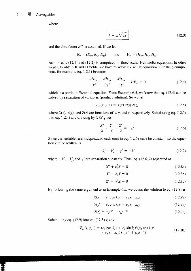
which is a partial differential equation. From Example 6.5, we know that eq. (12.4) can be

solved by separation of variables (product solution). So we let

Ezs(x, y, z) = X(x) Y(y) Z(z) (12.5)

where X(x), Y(y), and Z(z) are functions of*, y, and z, respectively. Substituting eq. (12.5)

into eq. (12.4) and dividing by XYZ gives

x" r z" 2— + — + — = -k2

X Y Z

(12.6)

Since the variables are independent, each term in eq. (12.6) must be constant, so the equa-

tion can be written as

-k\ - k) + y2 = -k2

(12.7)

where -k2, -k2, and y2 are separation constants. Thus, eq. (12.6) is separated as

X" + k2xX = 0 (12.8a)

r + k2yY = 0 (12.8b)

Z" - T2Z = 0 (12.8c)

By following the same argument as in Example 6.5, we obtain the solution to eq. (12.8) as

X(x) = c, cos k^x + c2 sin kyX

Y(y) = c3 cos kyy + c4 sin kyy

Z(z) = c5eyz + c6e'7Z

Substituting eq. (12.9) into eq. (12.5) gives

Ezs(x, y, z) = (ci cos kxx + c2 sin k^Xci, cos kyy

+ c4 sin kyy) (c5eyz + c6e~yz)

(12.9a)

(12.9b)

(12.9c)

(12.10)

12.2 RECTANGULAR WAVEGUIDES • 545

As usual, if we assume that the wave propagates along the waveguide in the +z-direction,

the multiplicative constant c5 = 0 because the wave has to be finite at infinity [i.e.,

Ezs(x, y, z = °°) = 0]. Hence eq. (12.10) is reduced to

Ezs(x, y, z) = (A; cos k^x + A2 sin cos kyy + A4 sin kyy)e (12.11)

where Aj = CiC6, A2 = c2c6, and so on. By taking similar steps, we get the solution of the

z-component of eq. (12.2) as

Hzs(x, y, z) = (Bi cos kpc + B2 sin ^ cos kyy + B4 sin kyy)e (12.12)

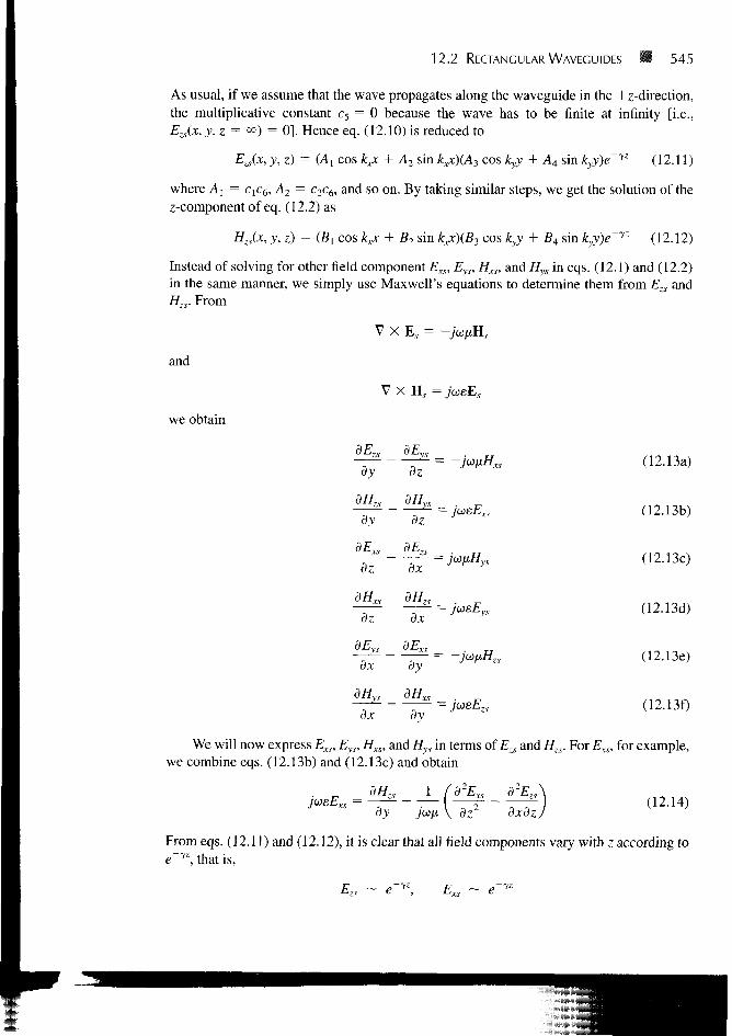
Instead of solving for other field component Exs, Eys, Hxs, and Hys in eqs. (12.1) and (12.2)

in the same manner, we simply use Maxwell's equations to determine them from Ezs and

HTS. From

and

V X E, = -y

V X H, = jtoeEs

we obtain

dE,<

dy

dHzs

dy

dExs

dz

dHxs

dz

dEys

dx

dHy,

dz

dHv,

dz

dx

dHz,

dx

9EX,

dy

dHx,

= jueExs

= J03flHys

dx dy

(12.13a)

(12.13b)

(12.13c)

(12.13d)

(12.13e)

(12.13f)

We will now express Exs, Eys, Hxs, and Hys in terms of Ezs and Hzs. For Exs, for example,

we combine eqs. (12.13b) and (12.13c) and obtain

dHz, 1 fd2Exs d2Ez.

dy 7C0/X \ dz oxdi(12.14)

From eqs. (12.11) and (12.12), it is clear that all field components vary with z according to

e~yz, that is,

p~lz F

546 • Waveguides

Hence

and eq. (12.14) becomes

dEzs d Exx ,

— = ~yEzs, —j- = 7 EX:

dZ dz

dHa 1 { 2 dE^jweExs = —— + - — I 7 Exs + 7——

dy joifi \ dx

or

1 , 2 , 2 ^ r 7 dEzs dHzs

—.— (7 + " V ) Exs = ~. — + ——jii ju>n dx dy

Thus, if we let h2 = y2 + w2/xe = y2 + k2,

E 1 —- '__7 dEzs jun dHzs

hl dx dy

Similar manipulations of eq. (12.13) yield expressions for Eys, Hxs, and Hys in terms of Ev

and Hzs. Thus,

(12.15a)

(12.15b)

(12.15c)

(12.15d)

Exs

EyS

M

Hys

h2 dx

7 dEzs

h2 dy

_ jue dEzs _

h2 dy

_ ja>e dEzs

jan dHz,

h2 dy

ju/x dHzs

h2 dx

7 dHzs

h2 dx

~~h2^T

where

h2 = y2 + k2 = k2x + k] (12.16)

Thus we can use eq. (12.15) in conjunction with eqs. (12.11) and (12.12) to obtain Exs, Eys,

Hxs, and Hys.

From eqs. (12.11), (12.12), and (12.15), we notice that there are different types of field

patterns or configurations. Each of these distinct field patterns is called a mode. Four dif-

ferent mode categories can exist, namely:

1. Ea = 0 = Hzs (TEM mode): This is the transverse electromagnetic (TEM) mode,

in which both the E and H fields are transverse to the direction of wave propaga-

tion. From eq. (12.15), all field components vanish for Ezs = 0 = Hzs. Conse-

quently, we conclude that a rectangular waveguide cannot support TEM mode.

12.3 TRANSVERSE MAGNETIC (TM) MODES 547

Figure 12.3 Components of EM fields in a rectangular waveguide:

(a) TE mode Ez = 0, (b) TM mode, Hz = 0.

2. Ezs = 0, Hzs # 0 (TE modes): For this case, the remaining components (Exs and

Eys) of the electric field are transverse to the direction of propagation az. Under this

condition, fields are said to be in transverse electric (TE) modes. See Figure

12.3(a).

3. Ezs + 0, Hzs = 0 (TM modes): In this case, the H field is transverse to the direction

of wave propagation. Thus we have transverse magnetic (TM) modes. See Figure

12.3(b).

4. Ezs + 0, Hzs + 0 (HE modes): This is the case when neither E nor H field is trans-

verse to the direction of wave propagation. They are sometimes referred to as

hybrid modes.

We should note the relationship between k in eq. (12.3) and j3 of eq. (10.43a). The

phase constant /3 in eq. (10.43a) was derived for TEM mode. For the TEM mode, h = 0, so

from eq. (12.16), y2 = -k2 -» y = a + j/3 = jk; that is, /3 = k. For other modes, j3 + k.

In the subsequent sections, we shall examine the TM and TE modes of propagation sepa-

rately.

2.3 TRANSVERSE MAGNETIC (TM) MODES

For this case, the magnetic field has its components transverse (or normal) to the direction

of wave propagation. This implies that we set Hz = 0 and determine Ex, Ey, Ez, Hx, and Hv

using eqs. (12.11) and (12.15) and the boundary conditions. We shall solve for Ez and later

determine other field components from Ez. At the walls of the waveguide, the tangential

components of the E field must be continuous; that is,

= 0 at y = 0

y = b£,, = 0 at

Ezs = 0 at x = 0

£„ = 0 at x = a

(12.17a)

(12.17b)

(12.17c)

(12.17d)

548 Waveguides

Equations (12.17a) and (12.17c) require that A, = 0 = A3 in eq. (12.11), so eq. (12.11)

becomes

Ea = Eo sin kj sin kyy e~yz (12.18)

where Eo = A2A4. Also eqs. (12.17b) and (12.17d) when applied to eq. (12.18) require that

s i n ^ = 0, sinkyb = O (12.19)

This implies that

kxa = rrnr, m = 1 , 2 , 3 , . . . (12.20a)

kyb = nir, n = 1 , 2 , 3 , . . . (12.20b)

or

_ n7r

Ky —

b

(12.21)

The negative integers are not chosen for m and n in eq. (12.20a) for the reason given in

Example 6.5. Substituting eq. (12.21) into eq. (12.18) gives

E7. = Eo sin. fnnrx\ . fniry\ 'in cm — \ o <c '

V aI sin

b ) '(12.22)

We obtain other field components from eqs. (12.22) and (12.15) bearing in mind that

H7< = 0. Thus

(12.23a)

(12.23b)

(12.23c)

y fnw\ IT • fmirx\ (n*y\ -yz

— ' — l F

o sin I I cos I I e T

jus

Hys = - v (-j-) Eo cos sin (12.23d)

where

nir(12.24)

which is obtained from eqs. (12.16) and (12.21). Notice from eqs. (12.22) and (12.23) that

each set of integers m and n gives a different field pattern or mode, referred to as TMmn

12.3 TRANSVERSE MAGNETIC (TM) MODES 549

mode, in the waveguide. Integer m equals the number of half-cycle variations in the x-

direction, and integer n is the number of half-cycle variations in the v-direction. We also

notice from eqs. (12.22) and (12.23) that if (m, n) is (0, 0), (0, n), or (m, 0), all field com-

ponents vanish. Thus neither m nor n can be zero. Consequently, TMH is the lowest-order

mode of all the TMmn modes.

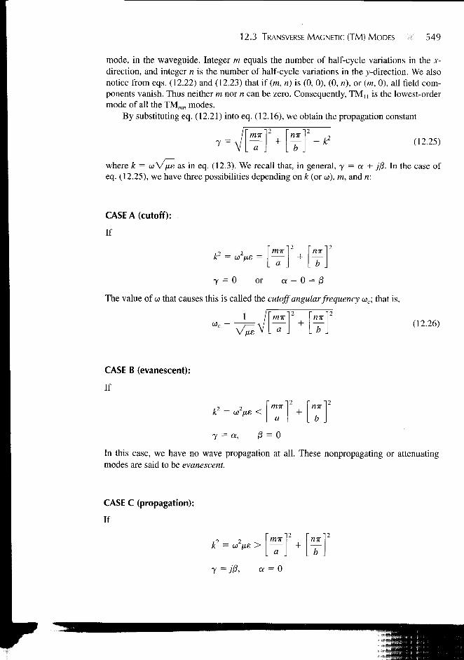
By substituting eq. (12.21) into eq. (12.16), we obtain the propagation constant

7 =mir

a

nir

b(12.25)

where k = u V ^ e as in eq. (12.3). We recall that, in general, y = a + j(3. In the case of

eq. (12.25), we have three possibilities depending on k (or w), m, and n:

CASE A (cutoff):

If

1c = w jus =[b

7 = 0 or a = 0 = /3

The value of w that causes this is called the cutoff angular frequency o)c; that is,

1 / U T T I 2 Tmr"12

I « J U (12.26)

CASE B (evanescent):

If

TOTTT]2 Tnir

y = a,

In this case, we have no wave propagation at all. These nonpropagating or attenuating

modes are said to be evanescent.

CASE C (propagation):

If

^2 = oA mir

y =;/?, a = 0

550 Waveguides

that is, from eq. (12.25) the phase constant (3 becomes

0 = - -L a nir(12.27)

This is the only case when propagation takes place because all field components will have

the factor e'yz = e~jl3z.

Thus for each mode, characterized by a set of integers m and n, there is a correspond-

ing cutoff frequency fc

The cutoff frequency is the operating frequencs below which allcnuaiion occurs

and above which propagation lakes place.

The waveguide therefore operates as a high-pass filter. The cutoff frequency is obtained

fromeq. (12.26) as

1

2-irVue

nnr

a

or

fcu

/ / N

// mu \)+ / N

/ nu\(12.28)

where u' = = phase velocity of uniform plane wave in the lossless dielectricfie

medium (a = 0, fi, e) filling the waveguide. The cutoff wave length \. is given by

or

X = (12.29)

Note from eqs. (12.28) and (12.29) that TMn has the lowest cutoff frequency (or the

longest cutoff wavelength) of all the TM modes. The phase constant /3 in eq. (12.27) can be

written in terms of fc as

= wV/xs^/ l - | -

12.3 TRANSVERSE MAGNETIC (TM) MODES 551

or

(12.30)

i

where j3' = oilu' = uVfie = phase constant of uniform plane wave in the dielectric

medium. It should be noted that y for evanescent mode can be expressed in terms of fc,

namely,

(12.30a)

The phase velocity up and the wavelength in the guide are, respectively, given by

w 2TT u \(12.31)

The intrinsic wave impedance of the mode is obtained from eq. (12.23) as (y = jfi)

Ex Ey

I T M -Hy Hx

we

or

»?TM = V (12.32)

where 17' = V/x/e = intrinsic impedance of uniform plane wave in the medium. Note the

difference between u', (3', and -q', and u, /3, and 77. The quantities with prime are wave

characteristics of the dielectric medium unbounded by the waveguide as discussed in

Chapter 10 (i.e., for TEM mode). For example, u' would be the velocity of the wave if

the waveguide were removed and the entire space were filled with the dielectric. The

quantities without prime are the wave characteristics of the medium bounded by the wave-

guide.

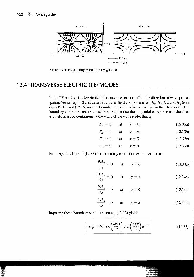
As mentioned before, the integers m and n indicate the number of half-cycle variations

in the x-y cross section of the guide. Thus for a fixed time, the field configuration of Figure

12.4 results for TM2, mode, for example.

552 Waveguides

end view

n= 1

E field

H field

Figure 12.4 Field configuration for TM2] mode.

side view

12.4 TRANSVERSE ELECTRIC (TE) MODES

In the TE modes, the electric field is transverse (or normal) to the direction of wave propa-

gation. We set Ez = 0 and determine other field components Ex, Ey, Hx, Hy, and Hz from

eqs. (12.12) and (12.15) and the boundary conditions just as we did for the TM modes. The

boundary conditions are obtained from the fact that the tangential components of the elec-

tric field must be continuous at the walls of the waveguide; that is,

Exs =

Exs '-

Eys =

Eys =

= 0

= 0

= 0

= 0

From eqs. (12.15) and (12.33), the boundary

dHzs

dy

dHzs

= 0

= 0

at

at

at

at

y = 0

y = b

x = 0

x — a

conditions can be written as

at

at

y-0

y = b

(12.33a)

(12.33b)

(12.33c)

(12.33d)

(12.34a)

(12.34b)dy

dHzs

dx

dHzs

dx

= 0

= 0

at

at

x = 0

x = a

Imposing these boundary conditions on eq. (12.12) yields

(m%x\ fmry\Hzs = Ho cos cos e yz

\ a ) \ b J

(12.34c)

(12.34d)

(12.35)

12.4 TRANSVERSE ELECTRIC (TE) MODES 553

where Ho = BXBT,. Other field components are easily obtained from eqs. (12.35) and

(12.15) as

) e

mrx

(12.36a)

(12.36b)

(12.36c)

(12.36d)

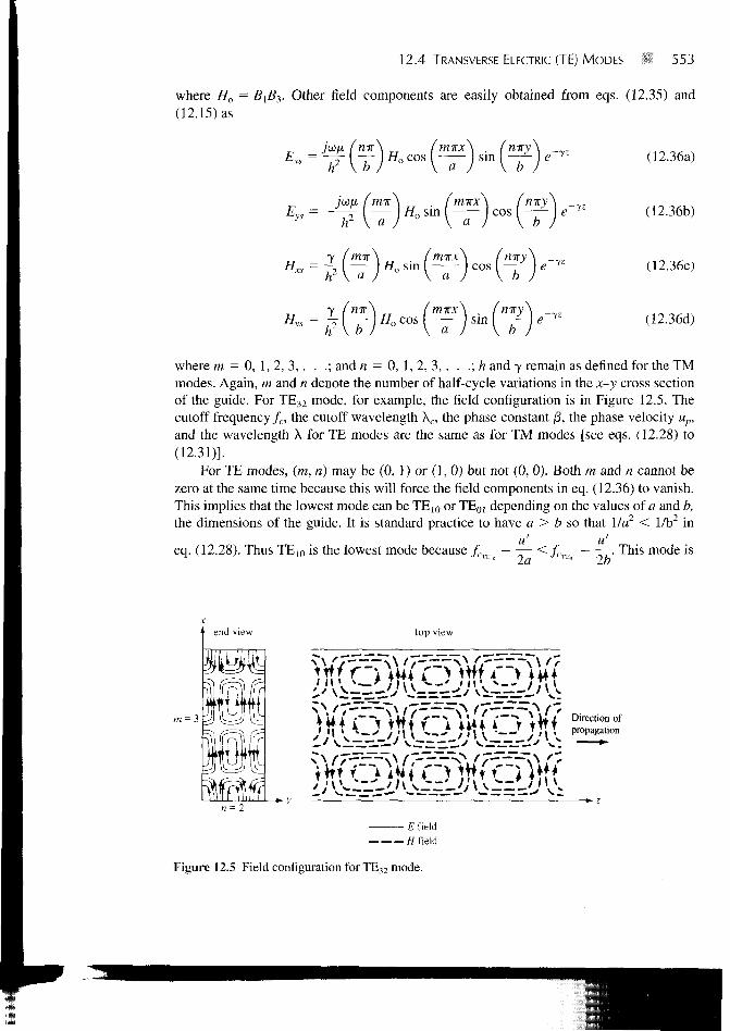
where m = 0, 1, 2, 3 , . . .; and n = 0, 1, 2, 3 , . . .; /J and 7 remain as defined for the TM

modes. Again, m and n denote the number of half-cycle variations in the x-y cross section

of the guide. For TE32 mode, for example, the field configuration is in Figure 12.5. The

cutoff frequency fc, the cutoff wavelength Xc, the phase constant /3, the phase velocity up,

and the wavelength X for TE modes are the same as for TM modes [see eqs. (12.28) to

(12.31)].

For TE modes, (m, ri) may be (0, 1) or (1, 0) but not (0, 0). Both m and n cannot be

zero at the same time because this will force the field components in eq. (12.36) to vanish.

This implies that the lowest mode can be TE10 or TE01 depending on the values of a and b,

the dimensions of the guide. It is standard practice to have a > b so that I/a2 < 1/b2 in

u' u'eq. (12.28). Thus TEi0 is the lowest mode because /CTE = — < /C.TK = —. This mode is

TE'° la Th°' 2b

top view

E field

//field

Figure 12.5 Field configuration for TE32 mode.

554 i§ Waveguides

called the dominant mode of the waveguide and is of practical importance. The cutoff fre-

quency for the TEH) mode is obtained from eq. (12.28) as (m = 1, n — 0)

Jc to 2a(12.37)

and the cutoff wavelength for TE]0 mode is obtained from eq. (12.29) as

Xt,0 = 2a (12.38)

Note that from eq. (12.28) the cutoff frequency for TMn is

u'[a2 + b2]1'2

2ab

which is greater than the cutoff frequency for TE10. Hence, TMU cannot be regarded as the

dominant mode.

The dominant mode is the mode with the lowest cutoff frequency (or longest cutoff

wavelength).

Also note that any EM wave with frequency / < fCw (or X > XC]0) will not be propagated in

the guide.

The intrinsic impedance for the TE mode is not the same as for TM modes. From

eq. (12.36), it is evident that (y = jf3)

Ex Ey (J)flr'

TE = jry = ~iTx

= T

Ifi 1

or

VTE I

V

12

J

(12.39)

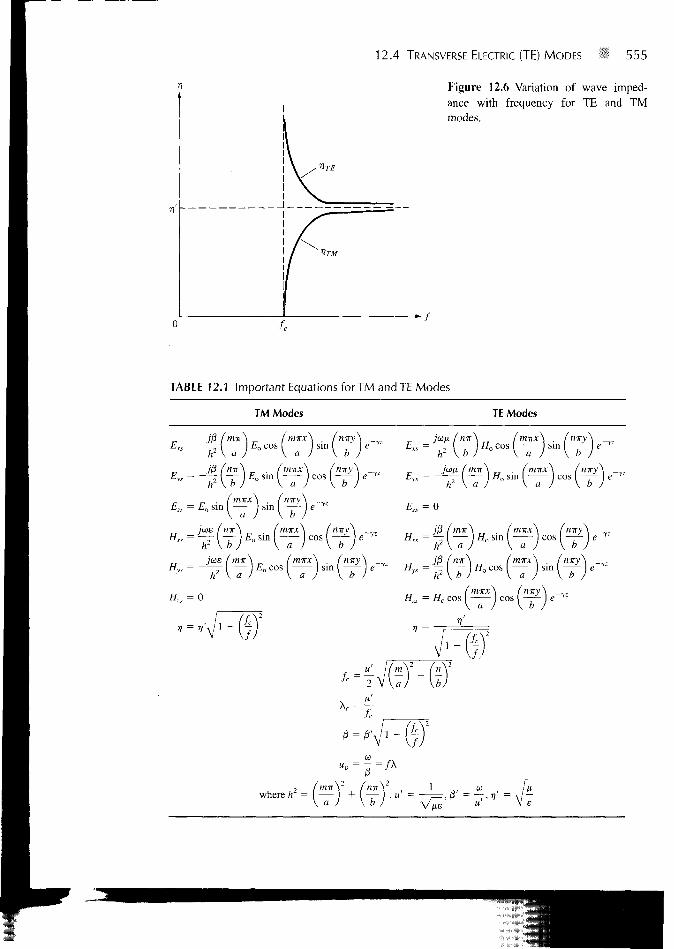
Note from eqs. (12.32) and (12.39) that r)TE and i?TM are purely resistive and they vary with

frequency as shown in Figure 12.6. Also note that

I?TE (12.40)

Important equations for TM and TE modes are listed in Table 12.1 for convenience and

quick reference.

12.4 TRANSVERSE ELECTRIC (TE) MODES 555

Figure 12.6 Variation of wave imped-

ance with frequency for TE and TM

modes.

TABLE 12.1 Important Equations for TM and TE Modes

TM Modes TE Modes

jP frmc\ fimrx\ . (n%y\ pn (rm\ fmirx\ . (rny\—r I Eo cos sin e 7 £„ = —— I — Ho cos I sin I e '~

h \ a J \ a J \ b J h \ b J \ a ) \ b JExs =

—- \ — )Eo sin | cos -—- ) e 7Z

a J \ b

\ / niryi I cos -—- | e

\ a J \ bEo sin I sin I — I e 1Z

\ a J \ b )jus

Ezs = 0

Hys = —yh \ a ) \ a ) V b

n*y i e-,,

. = 0

V =

j nnrx \ / rnryHzs = Ho cos cos —-x a V b

V =

where ^ = — + ^ . « ' =

556 Waveguides

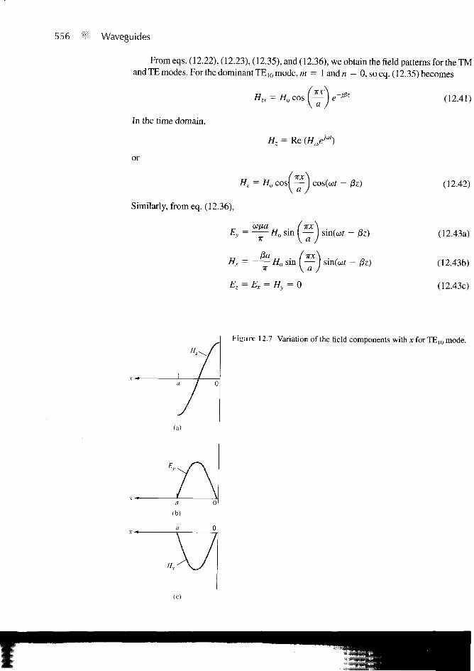
Fromeqs. (12.22), (12.23), (12.35), and (12.36), we obtain the field patterns for the TM

and TE modes. For the dominant TE]0 mode, m = landn = 0, so eq. (12.35) becomes

Hzs = Ho cos ( — | e -JPz

In the time domain,

Hz = Re (HzseM)

or

Hz = Ho cosf —

Similarly, from eq. (12.36),

= sin (

Hx = Ho sin ( —\a

- fiz)

(12.41)

(12.42)

(12.43a)

(12.43b)

(12.43c)

Figure 12.7 Variation of the field components with x for TE]0 mode.

(b)

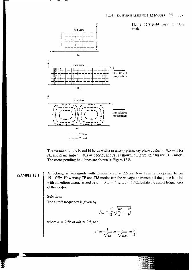
12.4 TRANSVERSE ELECTRIC (TE) MODES 557

Figure 12.8 Field lines for TE10

mode.

+ — Direction ofpropagation

top view

IfMi

'O

\ I^-•--x 1 - * - - N \ \

(c)

E field

//field

Direction ofpropagation

The variation of the E and H fields with x in an x-y plane, say plane cos(wf - |8z) = 1 for

Hz, and plane sin(of — j8z) = 1 for Ey and Hx, is shown in Figure 12.7 for the TE10 mode.

The corresponding field lines are shown in Figure 12.8.

EXAMPLE 12.1A rectangular waveguide with dimensions a = 2.5 cm, b = 1 cm is to operate below

15.1 GHz. How many TE and TM modes can the waveguide transmit if the guide is filled

with a medium characterized by a = 0, e = 4 so, /*,. = 1 ? Calculate the cutoff frequencies

of the modes.

Solution:

The cutoff frequency is given by

m2

where a = 2.5b or alb = 2.5, and

u =lie 'V-^r

558 Waveguides

Hence,

c

\~a3 X 108

4(2.5 X 10"Vm2 + 6.25M

2

or

fCmn = 3Vm2

GHz (12.1.1)

We are looking for fCnm < 15.1 GHz. A systematic way of doing this is to fix m or n

and increase the other until fCnm is greater than 15.1 GHz. From eq. (12.1.1), it is evident

that fixing m and increasing n will quickly give us an fCnm that is greater than 15.1 GHz.

ForTE01 mode (m = 0, n = 1), fCm = 3(2.5) = 7.5 GHz

TE02 mode (m = 0,n = 2),/Co2 = 3(5) = 15 GHz

TE03 mode,/Cm = 3(7.5) = 22.5 GHz

Thus for fCmn < 15.1 GHz, the maximum n = 2. We now fix n and increase m until fCmn is

greater than 15.1 GHz.

For TE10 mode (m = 1, n = 0), /C|o = 3 GHz

TE2o mode,/C20 = 6 GHz

TE30 mode,/C3o = 9 GHz

TE40mode,/C40 = 12 GHz

TE50 mode,/Cjo = 1 5 GHz (the same as for TE02)

TE60mode,/C60 = 18 GHz.

that is, for/Cn < 15.1 GHz, the maximum m = 5. Now that we know the maximum m and

n, we try other possible combinations in between these maximum values.

F o r T E n , T M n (degenerate modes), fCu = 3\/T25 = 8.078 GHz

TE21, TM2I,/C2i = 3V10.25 = 9.6 GHz

TE3],TM31,/C31 = 3Vl5 .25 = 11.72 GHz

TE41, TM41,/C4] = 3V22.25 = 14.14 GHz

TE12, TM12,/Ci, = 3V26 = 15.3 GHz

Those modes whose cutoff frequencies are less or equal to 15.1 GHz will be

transmitted—that is, 11 TE modes and 4 TM modes (all of the above modes except TE i2,

TM12, TE60, and TE03). The cutoff frequencies for the 15 modes are illustrated in the line

diagram of Figure 12.9.

12.4 TRANSVERSE ELECTRIC (TE) MODES S 559

TE4

TE,, TE30

9'

T E 3 TE41TE50,TE0

12 15• /c(GHz)

TMU TM21 TM31 TM41

Figure 12.9 Cutoff frequencies of rectangular waveguide with

a = 2.5b; for Example 12.1.

PRACTICE EXERCISE 12.1

Consider the waveguide of Example 12.1. Calculate the phase constant, phase veloc-

ity and wave impedance for TEi0 and TMu modes at the operating frequency of

15 GHz.

Answer: For TE10, (3 = 615.6rad/m, u = 1.531 X 108m/s, rjJE = 192.4 0. For

TMn,i3 = 529.4 rad/m, K = 1.78 X 108m/s,rjTM = 158.8 0.

EXAMPLE 12.2Write the general instantaneous field expressions for the TM and TE modes. Deduce those

for TEOi and TM12 modes.

Solution:

The instantaneous field expressions are obtained from the phasor forms by using

E = Re (EseJ'*) and H = Re (Hse

jo")

Applying these to eqs. (12.22) and (12.23) while replacing y and jfi gives the following

field components for the TM modes:

sm*=

iA ~r j E

°cos

j3\nw~\ fmirx\ fmry\= —A—-\EO sm cos —— si

\ a ) \ b J

(nvKx\ . fniryin cm IE7 = En sin

= --£ [T\ Eo sm

"z )

cos

560 • Waveguides

H =y h2

En cosI1 . (niry\ .

sin —— sm(a)t -a J \ b J

(3z)

Hz = 0

Similarly, for the TE modes, eqs. (12.35) and (12.36) become

E= —( mirx\ j mry\

, , Ho cos sin —— sin(ufb \ \ a J \ b J -Pz)

w/x fmir] . (m-wx\ frnry\ .= —r Ho sin cos si

h2 I a \ \ a J \ b J

7 = 0

Ho sin

/3 rn7r]Hy = ~2 [~\ Ho cos

fniry\cos —— sin(wr

b Icos

\ a J \ b I

j sin (-y) sin(.t -2 [ \ Ho cos ^ j

jm-wx\ fniry\H = Ho cos cos cos(co? - pz)

V a J \ b J

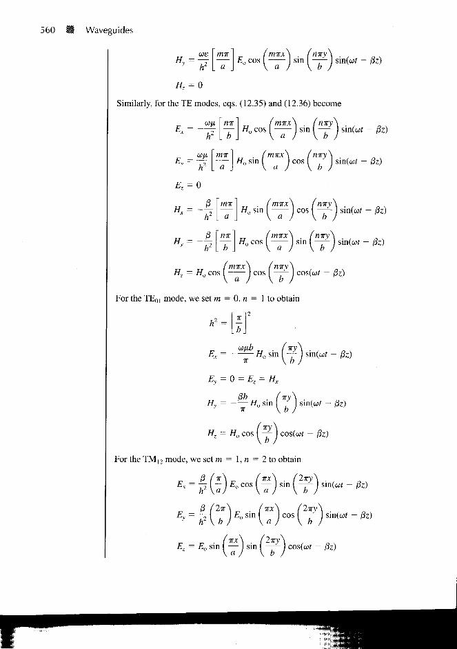
For the TE01 mode, we set m = 0, n = 1 to obtain

12

sin

hz= -

$bHy = - — //o sin

7T

iry\Hz = Ho cos I — I cos(cof - /3z)

\b J

For the TM|2 mode, we set m = 1, n = 2 to obtain

cin — cir(3 /TIA / X A . /27ry\ .

Ex = -j I - £o cos — sin — sin(cof - /3z)a / \ b

cos I —— I sir

(TTX\ (2iry\Ez = Eo sin — sin cos(o)f

V a J \ b J

12.4 TRANSVERSE ELECTRIC (TE) MODES 561

Hr = — 'o sin I — ) cos ( ^^ ] sin(cof - /3z)

o>e fir\ I\x\ . (2wy\Hy = —r — )EO cos — sin ~~— sm(ut -y h2 \aj \a J V b )

where

PRACTICE EXERCISE 12.2

An air-filled 5- by 2-cm waveguide has

Ezs = 20 sin 40irx sin 50?ry e"-"3" V/m

at 15 GHz.

(a) What mode is being propagated?

(b) Find |8.

(c) Determine EyIEx.

Answer: (a) TM2i, (b) 241.3 rad/m, (c) 1.25 tan 40wx cot 50-ry.

EXAMPLE 12.31 In a rectangular waveguide for which a = 1.5 cm, £ = 0.8 cm, a = 0, fi = JXO, and

e = 4eo,

Hx = 2 sin [ — ) cos sin (T X 10nt - 0z) A/m

Determine

(a) The mode of operation

(b) The cutoff frequency

(c) The phase constant /3

(d) The propagation constant y

(e) The intrinsic wave impedance 77.

Solution:

(a) It is evident from the given expression for Hx and the field expressions of the last

example that m = 1, n = 3; that is, the guide is operating at TMI3 or TE13. Suppose we

562 U Waveguides

choose TM13 mode (the possibility of having TE13 mode is left as an exercise in Practice

Exercise 12.3).

(b)

Hence

(c)

fcmn ~ 2 -

u =fiB

fca

1

4 V [1.5 x icr 2] 2 [0.8 x icr2]r2 ]2

(V0.444 + 14.06) X 102 = 28.57 GHz

L/Jfc

100co = 2TT/ = 7T X 10" or / = = 50 GHz

0 =3 X 10

s

(d) y =j0 = yl718.81/m

28.57

50= 1718.81 rad/m

(e) , = V

= 154.7

£12

/377 / _ I 28.5712

50

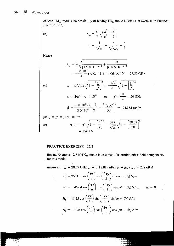
PRACTICE EXERCISE 12.3

Repeat Example 12.3 if TEn mode is assumed. Determine other field components

for this mode.

Answer: fc = 28.57 GHz, 0 = 1718.81 rad/m, ^ = ;/8, IJTE,, = 229.69 fi

£^ = 2584.1 cos ( — ) sin ( — ) sin(w/ - fa) V/m\a J \ b J

Ev = -459.4 sin | — ) cos ( — J sin(cor - fa) V/m,a J \ b J

= 0

= 11.25 cos (—) sin( \ / ̂ \TTJ: \ / 3;ry \— I sin —— Ia) V b J

sin(a>f - |8z) A/m

= -7.96 cos — cos — - cos (at - fa) A/m\ b J

12.5 WAVE PROPAGATION IN THE GUIDE 563

12.5 WAVE PROPAGATION IN THE GUIDE

Examination of eq. (12.23) or (12.36) shows that the field components all involve the

terms sine or cosine of (mi/a)i or (nirlb)y times e~yz. Since

sin 6» = — (eje - e~i6)2/

cos 6 = - (eje + e jB)

(12.44a)

(12.44b)

a wave within the waveguide can be resolved into a combination of plane waves reflected

from the waveguide walls. For the TE]0 mode, for example,

(12.45)

c* = ~Hj*-J"

2x _

The first term of eq. (12.45) represents a wave traveling in the positive z-direction at an

angle

= tan (12.46)

with the z-axis. The second term of eq. (12.45) represents a wave traveling in the positive

z-direction at an angle —6. The field may be depicted as a sum of two plane TEM waves

propagating along zigzag paths between the guide walls at x = 0 and x = a as illustrated

in Figure 12.10(a). The decomposition of the TE!0 mode into two plane waves can be ex-

tended to any TE and TM mode. When n and m are both different from zero, four plane

waves result from the decomposition.

The wave component in the z-direction has a different wavelength from that of the

plane waves. This wavelength along the axis of the guide is called the waveguide wave-

length and is given by (see Problem 12.13)

X =X'

(12.47)

where X' = u'/f.

As a consequence of the zigzag paths, we have three types of velocity: the medium ve-

locity u', the phase velocity up, and the group velocity ug. Figure 12.10(b) illustrates the re-

lationship between the three different velocities. The medium velocity u' = 1/V/xe is as

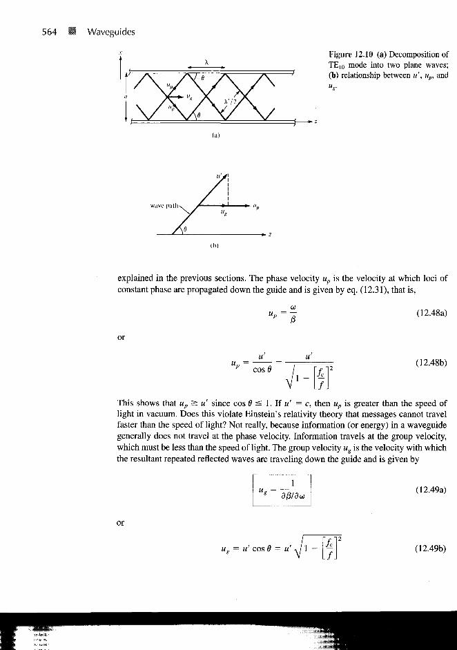
564 Waveguides

Figure 12.10 (a) Decomposition of

TE10 mode into two plane waves;

(b) relationship between u', up, and

(a)

wave path

(ID

explained in the previous sections. The phase velocity up is the velocity at which loci of

constant phase are propagated down the guide and is given by eq. (12.31), that is,

«„ = 7T d2.48a)

or

Up cos e(12.48b)

This shows that up > u' since cos 6 < 1. If u' = c, then up is greater than the speed of

light in vacuum. Does this violate Einstein's relativity theory that messages cannot travel

faster than the speed of light? Not really, because information (or energy) in a waveguide

generally does not travel at the phase velocity. Information travels at the group velocity,

which must be less than the speed of light. The group velocity ug is the velocity with which

the resultant repeated reflected waves are traveling down the guide and is given by

(12.49a)

or

uo = u' cos 6 = u' (12.49b)

12.6 POWER TRANSMISSION AND ATTENUATION 565

Although the concept of group velocity is fairly complex and is beyond the scope of this

chapter, a group velocity is essentially the velocity of propagation of the wave-packet en-

velope of a group of frequencies. It is the energy propagation velocity in the guide and is

always less than or equal to u'. From eqs. (12.48) and (12.49), it is evident that

upug = u'2 (12.50)

This relation is similar to eq. (12.40). Hence the variation of up and ug with frequency is

similar to that in Figure 12.6 for r;TE and rjTM.

EXAMPLE 12.4A standard air-filled rectangular waveguide with dimensions a = 8.636 cm, b = 4.318 cm

is fed by a 4-GHz carrier from a coaxial cable. Determine if a TE10 mode will be propa-

gated. If so, calculate the phase velocity and the group velocity.

Solution:

For the TE10 mode, fc = u' 11a. Since the waveguide is air-filled, u' = c = 3 X 108.

Hence,

fc =3 X 10*

= 1.737 GHz2 X 8.636 X 10~

2

As / = 4 GHz > fc, the TE10 mode will propagate.

u' 3 X 108

V l - (fjff V l - (1.737/4)2

= 3.33 X 108 m/s

16

g

9 X 10j

3.33 X 108

= 2.702 X 108 m/s

PRACTICE EXERCISE 12.4

Repeat Example 12.4 for the TM n mode.

Answer: 12.5 X 108 m/s, 7.203 X 10

7 m/s.

12.6 POWER TRANSMISSION AND ATTENUATION

To determine power flow in the waveguide, we first find the average Poynting vector [from

eq. (10.68)],

(12.51)

566 • Waveguides

In this case, the Poynting vector is along the z-direction so that

1

_ \Ea-\2 + \Eys\

2

2V

(12.52)

where rj = rjTE for TE modes or 77 = »/TM for TM modes. The total average power trans-

mitted across the cross section of the waveguide is

— \ at, . J C

(12.53)

- dy dx

=0 Jy=0

Of practical importance is the attenuation in a lossy waveguide. In our analysis thus

far, we have assumed lossless waveguides (a = 0, ac — °°) for which a = 0, 7 = j/3.

When the dielectric medium is lossy (a # 0) and the guide walls are not perfectly con-

ducting (ac =£ 00), there is a continuous loss of power as a wave propagates along the

guide. According to eqs. (10.69) and (10.70), the power flow in the guide is of the form

P = P e -2az (12.54)

In order that energy be conserved, the rate of decrease in Pave must equal the time average

power loss PL per unit length, that is,

P L = -dPa.

dz

or

^ • * fl

In general,

= ac ad

(12.55)

(12.56)

where ac and ad are attenuation constants due to ohmic or conduction losses (ac # 00) and

dielectric losses (a ¥= 0), respectively.

To determine ad, recall that we started with eq. (12.1) assuming a lossless dielectric

medium (a = 0). For a lossy dielectric, we need to incorporate the fact that a =£ 0. All our

equations still hold except that 7 = jj3 needs to be modified. This is achieved by replacing

e in eq. (12.25) by the complex permittivity of eq. (10.40). Thus, we obtain

mir\ frnr\2 2

(12.57)

12.6 POWER TRANSMISSION AND ATTENUATION 567

where

ec = e' - je" = s - j - (12.58)CO

Substituting eq. (12.58) into eq. (12.57) and squaring both sides of the equation, we obtain

2 27 = ad 2 f t A = l - ^ ) +[~) -S

fiir

Equating real and imaginary parts,

\ a+ \T)

(12.59a)

2adf3d = co/xa or ad =

Assuming that ad <£. (3d, azd - j3z

d = -/3J, so eq. (12.59a) gives

a )

(12.59b)

(12.60)

which is the same as (3 in eq. (12.30). Substituting eq. (12.60) into eq. (12.59b) gives

(12.61)

where rj' = V/x/e.

The determination of ac for TMmn and TEmn modes is time consuming and tedious. We

shall illustrate the procedure by finding ac for the TE10 mode. For this mode, only Ey, Hx,

and Hz exist. Substituting eq. (12.43a) into eq. (12.53) yields

a f b

- dxdy =x=0 Jy=

2ir r)dy sin — dx

'° ° a (12.62)

* ave

The total power loss per unit length in the walls is

y=o

\y=b + Pi \X=0

=O)(12.63)

568 Waveguides

since the same amount is dissipated in the walls y = 0 and y = b or x = 0 and x = a. For

the wall y = 0,

TJC j {\Hxs\l+ \Hzs\

z)dx

a #2 27TJC

H2nsin2 — Hz

o cos1 — dx\ (12.64)

£ 1 +

7T

where Rs is the real part of the intrinsic impedance t\c of the conducting wall. From eq.

(10.56),

1

ar8(12.65)

where 5 is the skin depth. Rs is the skin resistance of the wall; it may be regarded as the re-

sistance of 1 m by 5 by 1 m of the conducting material. For the wall x = 0,

C I (\Hzs\z)dy H2

ody

RJbHl(12.66)

Substituting eqs. (12.64) and (12.66) into eq. (12.63) gives

(12.67)

Finally, substituting eqs. (12.62) and (12.67) into eq. (12.55),

?2 2

2ir r/

ar = (12.68a)

It is convenient to express ac. in terms of/ and fc. After some manipulations, we obtain for

the TE10 mode

2RS kL/

(12.68b)

12.7 WAVEGUIDE CURRENT AND MODE EXCITATION 569

By following the same procedure, the attenuation constant for the TEm« modes (n + 0) can

be obtained as

(12.69)

r

md for the TMmn

-'fc

J.

2(l 1I

modes as

" c TM

OH2

2/?,

2 m

(bid?

'fViblaf

, 2

+ n2

m2 +

m2 +

kV

n2 \

\f<}2)[f\)

(12.70)

The total attenuation constant a is obtained by substituting eqs. (12.61) and (12.69) or

(12.70) into eq. (12.56).

12.7 WAVEGUIDE CURRENT AND MODE EXCITATION

For either TM or TE modes, the surface current density K on the walls of the waveguide

may be found using

K = an X H (12.71)

where an is the unit outward normal to the wall and H is the field intensity evaluated on the

wall. The current flow on the guide walls for TE10 mode propagation can be found using

eq. (12.71) with eqs. (12.42) and (12.43). The result is sketched in Figure 12.11.

The surface charge density ps on the walls is given by

ps = an • D = an • eE

where E is the electric field intensity evaluated on the guide wall.

(12.72)

Figure 12.11 Surface current on guidewalls for TE10 mode.

570 Waveguides

?"\

J

(a) TE,n mode.

0 a 0

(b)TMM mode.

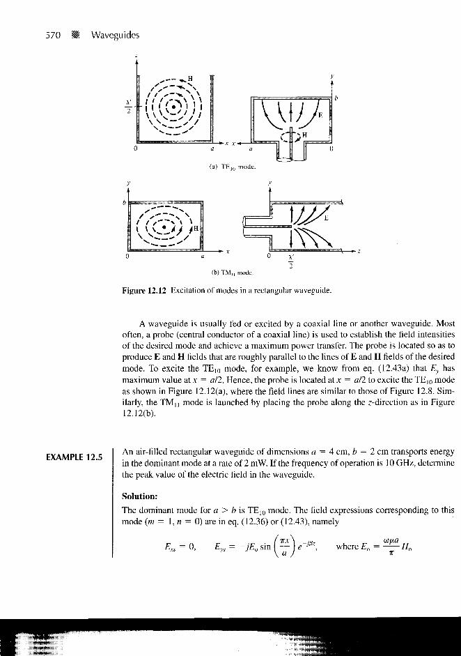
Figure 12.12 Excitation of modes in a rectangular waveguide.

A waveguide is usually fed or excited by a coaxial line or another waveguide. Most

often, a probe (central conductor of a coaxial line) is used to establish the field intensities

of the desired mode and achieve a maximum power transfer. The probe is located so as to

produce E and H fields that are roughly parallel to the lines of E and H fields of the desired

mode. To excite the TE10 mode, for example, we know from eq. (12.43a) that Ey has

maximum value at x = ail. Hence, the probe is located at x = a/2 to excite the TEIO mode

as shown in Figure 12.12(a), where the field lines are similar to those of Figure 12.8. Sim-

ilarly, the TMii mode is launched by placing the probe along the z-direction as in Figure

EXAMPLE 12.5An air-filled rectangular waveguide of dimensions a = 4 cm, b = 2 cm transports energy

in the dominant mode at a rate of 2 mW. If the frequency of operation is 10 GHz, determine

the peak value of the electric field in the waveguide.

Solution:

The dominant mode for a > b is TE10 mode. The field expressions corresponding to this

mode (m = 1, n = 0) are in eq. (12.36) or (12.43), namely

Exs = 0, Eys = -jE0 sin ( — where £„ =

12.7 WAVEGUIDE CURRENT AND MODE EXCITATION I I 571

Jc 2a 2(4 X 10~2)

V' 377

/ c

= 406.7

1 -3.75

. / J V L io

From eq. (12.53), the average power transmitted is

P = r r \Mave L L 2^

Hence,

dy

4r,

2t, —

4(406.7) X 2 X 1Q"3

ab 8 X 10

En = 63.77 V/m

= 4067

PRACTICE EXERCISE 12.5

In Example 12.5, calculate the peak value Ho of the magnetic field in the guide if

a = 2 cm, b = 4 cm while other things remain the same.

Answer: 63.34 mA/m.

EXAMPLE 12.6A copper-plated waveguide (ac = 5.8 X 10

7 S/m) operating at 4.8 GHz is supposed to

deliver a minimum power of 1.2 kW to an antenna. If the guide is filled with polystyrene

(a = 10"17

S/m, e = 2.55eo) and its dimensions are a = 4.2 cm, b = 2.6 cm, calculate

the power dissipated in a length 60 cm of the guide in the TE10 mode.

Solution:

Let

Pd = power loss or dissipated

Pa = power delivered to the antenna

Po = input power to the guide

so that P0 = Pd + Pa

Fromeq. (12.54),

D — D ,,~2<xz

572 Waveguides

Hence,

Pa =-2az

or

Now we need to determine a from

From eq. (12.61),

= Pa(elaz - 1)

a = ad + ac

or,'

Since the loss tangent

10 -17

ue q 10~9

2x X 4.8 X 109 X X 2.5536TT

then

= 1.47 X 10"17 « : 1 (lossless dielectric medium)

= 236.1

= 1.879 X 108m/sBr

2a 2 X 4.2 X 10'

10~17

X 236.1

2.234 GHz

/ _ [2.23412

L 4 .8 Jad = 1.334 X 10~15Np/m

For the TE10 mode, eq. (12.68b) gives

ar =

V2

If

0.5 + - kL/J

12.7 WAVEGUIDE CURRENT AND MODE EXCITATION 573

where

Hence

/?. =ac8

= 1.808 X 10~2Q

1 hrfiJ. hrX 4.8 X 109 X 4ir X 10

- 7

5.8 X 107

2 X l i

a, =

2.6 X1O"2X 236

= 4.218 X 10"3Np/m

/. 1 ^ 1 -

234

Note that ad <§C ac, showing that the loss due to the finite conductivity of the guide walls

is more important than the loss due to the dielectric medium. Thus

a = ad + ac = ac = 4.218 X 10"3 Np/m

and the power dissipated is

= 6.089 W

Pd = Pa{e^ _ i) = 1.2 x ioVx 4 -

2 1 8 x l o"x a 6 - 1)

PRACTICE EXERCISE 12.6

A brass waveguide (ac = 1.1 X 107 mhos/m) of dimensions a = 4.2 cm, b —

1.5 cm is filled with Teflon (er = 2.6, a = 10"15

mhos/m). The operating frequency

is 9 GHz. For the TE10 mode:

(a) Calculate <xd and ac.

(b) What is the loss in decibels in the guide if it is 40 cm long?

Answer: (a) 1.206 X 10~iJ Np/m, 1.744 X 10~

zNp/m, (b) 0.0606 dB.

EXAMPLE 12.7Sketch the field lines for the TMn mode. Derive the instantaneous expressions for the

surface current density of this mode.

Solution:

From Example 12.2, we obtain the fields forTMn mode (m = 1, n = 1) as

Ey = Ti i j;) Eo s i n ( ~ ) c o s ( y ) sin(cof - j3z)

574 Waveguides

Ez = Eo sin I — I sin I — I cos(wr - /3z)x a J \ b J

we / TT \ I %x \ iry\Hx = —-j I — £o sin I — I cos I —- sin(wf -

h \bj \a I \ b

we /vr\y = ~tf \a)

E°(TXX

Va

//, = 0

For the electric field lines,

dy E., a firx\ (%y— = - r = 7 tan — cot —cfx £x b \a I \b

For the magnetic field lines,

dy Hy b /TTX\

dx Hx a \ a Jiry \

b J

Notice that (Ey/Ex)(Hy/Hx) = — 1, showing that electric and magnetic field lines are mutu-

ally orthogonal. This should also be observed in Figure 12.13 where the field lines are

sketched.

The surface current density on the walls of the waveguide is given by

K = an X H = a* X (Hx, Hy, 0)

At x = 0, an = ax, K = Hy(0, y, z, t) az, that is,

we fir

At x = a, an = -a x , K = -Hy(a, y, z, i) az

or

Tr we (ir

1? \a

Figure 12.13 Field lines for TMU mode; forExample 12.7.

E field

H field

12.8 WAVEGUIDE RESONATORS 575

At y = 0, an = ay, K = -Hx(x, 0, z, t) az

or

Aty = b,an = -ay, K = Hx(x, b, z, t) az

or

COS / 7T \ / TTX ,K = — I — ) Eo sin — sm(atf - j3z) az

h \bj \ a

- I3z) az

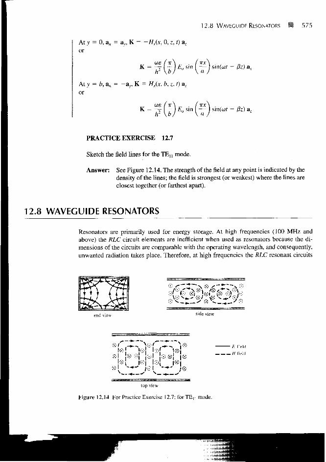
PRACTICE EXERCISE 12.7

Sketch the field lines for the TE n mode.

Answer: See Figure 12.14. The strength of the field at any point is indicated by the

density of the lines; the field is strongest (or weakest) where the lines are

closest together (or farthest apart).

12.8 WAVEGUIDE RESONATORS

Resonators are primarily used for energy storage. At high frequencies (100 MHz and

above) the RLC circuit elements are inefficient when used as resonators because the di-

mensions of the circuits are comparable with the operating wavelength, and consequently,

unwanted radiation takes place. Therefore, at high frequencies the RLC resonant circuits

end view side view

U J©i ©^

©| !©[

E field

//field

top view

Figure 12.14 For Practice Exercise 12.7; for TEn mode.

576 Waveguides

are replaced by electromagnetic cavity resonators. Such resonator cavities are used in kly-

stron tubes, bandpass filters, and wave meters. The microwave oven essentially consists of

a power supply, a waveguide feed, and an oven cavity.

Consider the rectangular cavity (or closed conducting box) shown in Figure 12.15. We

notice that the cavity is simply a rectangular waveguide shorted at both ends. We therefore

expect to have standing wave and also TM and TE modes of wave propagation. Depending

on how the cavity is excited, the wave can propagate in the x-, y-, or z-direction. We will

choose the +z-direction as the "direction of wave propagation." In fact, there is no wave

propagation. Rather, there are standing waves. We recall from Section 10.8 that a standing

wave is a combination of two waves traveling in opposite directions.

A. TM Mode to z

For this case, Hz = 0 and we let

EJx, y, z) = X(x) Y(y) Z(z) (12.73)

be the production solution of eq. (12.1). We follow the same procedure taken in Section12.2 and obtain

X(x) = C\ cos kjX + c2 sin kpc

Y(y) = c3 cos kyy + c4 sin kyy

Z(z) = c5 cos kzz + c6 sin kzz,

where

k2 = k2x + k], + k] = u2ixe

The boundary conditions are:

£z = 0 at x = 0, a

Ez = 0 at >' = 0 ,6

Ey = 0,Ex = 0 at z = 0, c

(12.74a)

(12.74b)

(12.74c)

(12.75)

(12.76a)

(12.76b)

(12.76c)

Figure 12.15 Rectangular cavity.

12.8 WAVEGUIDE RESONATORS • 577

As shown in Section 12.3, the conditions in eqs. (12.7a, b) are satisfied when

cx = 0 = c3 and

nvK

a y b(12.77)

where m = 1, 2, 3, . . ., n = 1, 2, 3, . . . .To invoke the conditions in eq. (12.76c), we

notice that eq. (12.14) (with Hzs = 0) yields

d2Exs d2Ezs

dz dz

Similarly, combining eqs. (12.13a) and (12.13d) (with Hzs = 0) results in

-ycoe ys -

From eqs. (12.78) and (12.79), it is evident that eq. (12.76c) is satisfied if

— - = 0 at z = 0, cdz

This implies that c6 = 0 and sin kzc = 0 = sin pir. Hence,

(12.78)

(12.79)

(12.80)

(12.81)

where p = 0, 1, 2, 3 , . . . . Substituting eqs. (12.77) and (12.81) into eq. (12.74) yields

(12.82)

where Eo = c2c4c5. Other field components are obtained from eqs. (12.82) and (12.13).

The phase constant /3 is obtained from eqs. (12.75), (12.77), and (12.81) as

(12.83)

Since /32 = co

2/i£, from eq. (12.83), we obtain the resonant frequency fr

2irfr = ur =fie

or

ufr ^

/r i/ w

[a\

2 r 12

" 1 Ir "

r (12.84)

578 • Waveguides

The corresponding resonant wavelength is

u'

" fr llm

VUrJ

2

In

L ^f +1 UJ

9(12.85)

From eq. (12.84), we notice that the lowest-order TM mode is TM110-

B. TE Mode to z

In this case, Ez = 0 and

Hzs = (bt cos sin 3 cos kyy + b4 sin kyy)

(^5 cos kzz + sin kzz)

The boundary conditions in eq. (12.76c) combined with eq. (12.13) yields

at z = 0, cHzs =

dx

dy

= 0 at x = 0, a

= 0 at = 0,b

(12.86)

(12.87a)

(12.87b)

(12.87c)

Imposing the conditions in eq. (12.87) on eq. (12.86) in the same manner as for TM mode

to z leads to

(12.88)

where m = 0, 1, 2, 3, . . ., n = 0, 1, 2, 3, . . ., and p = 1, 2, 3, . . . . Other field com-

ponents can be obtained from eqs. (12.13) and (12.88). The resonant frequency is the

same as that of eq. (12.84) except that m or n (but not both at the same time) can be

zero for TE modes. The reason why m and n cannot be zero at the same time is that the

field components will be zero if they are zero. The mode that has the lowest resonant

frequency for a given cavity size (a, b, c) is the dominant mode. If a > b < c, it implies

that I/a < \lb > lie and hence the dominant mode is TE101. Note that for a > b < c, the

resonant frequency of TMU0 mode is higher than that for TE101 mode; hence, TE101 is

dominant. When different modes have the same resonant frequency, we say that the

modes are degenerate; one mode will dominate others depending on how the cavity is

excited.

A practical resonant cavity has walls with finite conductivity ac and is, therefore,

capable of losing stored energy. The quality factor Q is a means of determining the loss.

12.8 WAVEGUIDE RESONATORS 579

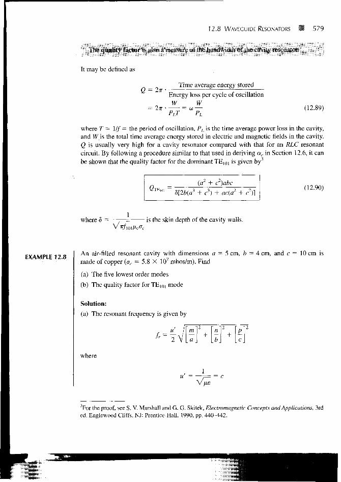
The qiialitx factor is also a measure of I he bandwidth ol' the cavity resonator.

It may be defined as

Time average energy stored

Energy loss per cycle of oscillation

W W(12.89)

where T = 1// = the period of oscillation, PL is the time average power loss in the cavity,

and W is the total time average energy stored in electric and magnetic fields in the cavity.

Q is usually very high for a cavity resonator compared with that for an RLC resonant

circuit. By following a procedure similar to that used in deriving ac in Section 12.6, it can

be shown that the quality factor for the dominant TE]01 is given by3

GTE 1 0 1 =5[2b(a3

(a2

+ c

+3)

c2)abc

+ acia fc!)](12.90)

where 5 = is the skin depth of the cavity walls.

EXAMPLE 12.8An air-filled resonant cavity with dimensions a = 5 cm, b = 4 cm, and c = 10 cm is

made of copper (oc = 5.8 X 107 mhos/m). Find

(a) The five lowest order modes

(b) The quality factor for TE1Oi mode

Solution:

(a) The resonant frequency is given by

m

where

u' = = c

3For the proof, see S. V. Marshall and G. G. Skitek, Electromagnetic Concepts and Applications, 3rd

ed. Englewood Cliffs, NJ: Prentice-Hall, 1990, pp. 440-442.

580 S Waveguides

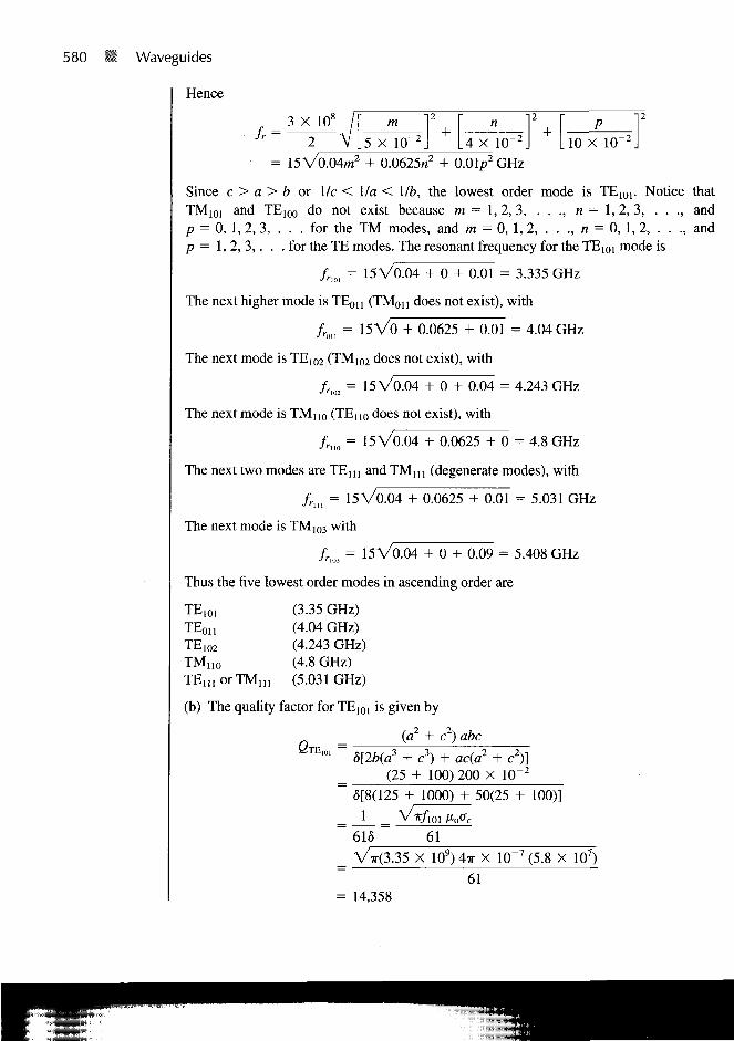
Hence

3 X l(f m5 X 10" 4 X 10

- 210 X 10

- 2

= 15V0.04m2 + 0.0625«

2 + 0.01/?

2 GHz

Since c > a > b or 1/c < I/a < 1/&, the lowest order mode is TE101. Notice that

TMioi and TE1Oo do not exist because m = 1,2, 3, . . ., n = 1,2, 3, . . ., and

p = 0, 1, 2, 3, . . . for the TM modes, and m = 0, 1, 2, . . ., n = 0, 1, 2, . . ., and

p = 1,2,3,. . . for the TE modes. The resonant frequency for the TE1Oi mode is

frm = 15V0.04 + 0 + 0.01 = 3.335 GHz

The next higher mode is TE011 (TM011 does not exist), with

fron = 15V0 + 0.0625 + 0.01 = 4.04 GHz

The next mode is TE102 (TM!02 does not exist), with

frim = 15V0.04 + 0 + 0.04 = 4.243 GHz

The next mode is TM110 (TE110 does not exist), with

fruo = 15V0.04 + 0.0625 + 0 = 4.8 GHz

The next two modes are TE i n and TM n ] (degenerate modes), with

frni = 15V0.04 + 0.0625 + 0.01 = 5.031 GHz

The next mode is TM103 with

frm = 15V0.04 + 0 + 0.09 = 5.408 GHz

Thus the five lowest order modes in ascending order are

TE101 (3.35 GHz)

TEon (4.04 GHz)

TE102 (4.243 GHz)

TMU 0 (4.8 GHz)

T E i , , o r T M i n (5.031 GHz)

(b) The quality factor for TE]01 is given by

2TEI01 -(a2 c2) abc

S[2b(a c3) ac(a2 c2)]

(25 + 100) 200 X 10~2

5[8(125 + 1000) + 50(25 + 100)]

616 61

VV(3.35 X 109) 4TT X 10"7 (5.8 X 107)

61

= 14,358

SUMMARY 581

PRACTICE EXERCISE 12.8

If the resonant cavity of Example 12.8 is filled with a lossless material (/xr = 1,

er - 3), find the resonant frequency fr and the quality factor for TE101 mode.

Answer: 1.936 GHz, 1.093 X 104

SUMMARY 1. Waveguides are structures used in guiding EM waves at high frequencies. Assuming a

lossless rectangular waveguide (ac — o°, a — 0), we apply Maxwell's equations in ana-

lyzing EM wave propagation through the guide. The resulting partial differential equa-

tion is solved using the method of separation of variables. On applying the boundary

conditions on the walls of the guide, the basic formulas for the guide are obtained for

different modes of operation.

2. Two modes of propagation (or field patterns) are the TMmn and TEmn where m and n are

positive integers. For TM modes, m = 1, 2, 3, . . ., and n = 1, 2, 3, . . . and for TE

modes, m = 0, 1, 2, . . ., and n = 0, 1, 2, . . .,n = m¥z0.

3. Each mode of propagation has associated propagation constant and cutoff frequency.

The propagation constant y = a + jfl does not only depend on the constitutive pa-

rameters (e, /x, a) of the medium as in the case of plane waves in an unbounded space,

it also depends on the cross-sectional dimensions (a, b) of the guide. The cutoff fre-

quency is the frequency at which y changes from being purely real (attenuation) to

purely imaginary (propagation). The dominant mode of operation is the lowest mode

possible. It is the mode with the lowest cutoff frequency. If a > b, the dominant mode

is TE10.

4. The basic equations for calculating the cutoff frequency fc, phase constant 13, and phase

velocity u are summarized in Table 12.1. Formulas for calculating the attenuation con-

stants due to lossy dielectric medium and imperfectly conducting walls are also pro-

vided.

5. The group velocity (or velocity of energy flow) ug is related to the phase velocity up of

the wave propagation by

upug = u'2

where u' = 1/v/xs is the medium velocity—i.e., the velocity of the wave in the di-

electric medium unbounded by the guide. Although up is greater than u', up does not

exceed u'.

6. The mode of operation for a given waveguide is dictated by the method of exci-

tation.

7. A waveguide resonant cavity is used for energy storage at high frequencies. It is nothing

but a waveguide shorted at both ends. Hence its analysis is similar to that of a wave-

guide. The resonant frequency for both the TE and TM modes to z is given by

m

582 Waveguides

For TM modes, m = 1, 2, 3, . . ., n = 1, 2, 3, . . ., and p = 0, 1, 2, 3, . . ., and for

TE modes, m = 0,1,2,3,. . ., n = 0, 1, 2, 3 , . . ., and p = 1, 2, 3 , . . .,m = n ^ 0.

If a > b < c, the dominant mode (one with the lowest resonant frequency) is TE1Oi-

8. The quality factor, a measure of the energy loss in the cavity, is given by

2 = "-?

12.1 At microwave frequencies, we prefer waveguides to transmission lines for transporting

EM energy because of all the following except that

(a) Losses in transmission lines are prohibitively large.

(b) Waveguides have larger bandwidths and lower signal attenuation.

(c) Transmission lines are larger in size than waveguides.

(d) Transmission lines support only TEM mode.

12.2 An evanscent mode occurs when

(a) A wave is attenuated rather than propagated.

(b) The propagation constant is purely imaginary.

(c) m = 0 = n so that all field components vanish.

(d) The wave frequency is the same as the cutoff frequency.

12.3 The dominant mode for rectangular waveguides is

(a) TE,,

(b) TM n

(c) TE1Oi

(d) TE10

12.4 The TM10 mode can exist in a rectangular waveguide.

(a) True

(b) False

12.5 For TE30 mode, which of the following field components exist?

(a) Ex

(b) Ey

(c) Ez

(d) Hx

(e) Hv

PROBLEMS 583

12.6 If in a rectangular waveguide for which a = 2b, the cutoff frequency for TE02 mode is12 GHz, the cutoff frequency for TMH mode is

(a) 3 GHz

(b) 3 \ /5GHz

(c) 12 GHz

(d) 6 \A GHz

(e) None of the above

12.7 If a tunnel is 4 by 7 m in cross section, a car in the tunnel will not receive an AM radiosignal (e.g.,/= 10 MHz).

(a) True

(b) False

12.8 When the electric field is at its maximum value, the magnetic energy of a cavity is

(a) At its maximum value

(b) At V 2 of its maximum value

(c) At —-p of its maximum value

V 2

(d) At 1/2 of its maximum value

(e) Zero

12.9 Which of these modes does not exist in a rectangular resonant cavity?

(a) TE110

(b) TEQH

(c) TM110

(d) TMm

12.10 How many degenerate dominant modes exist in a rectangular resonant cavity for whicha = b = c?

(a) 0

(b) 2

(c) 3

(d) 5

(e) oo

Answers: 12.1c, 12.2a, 12.3d, 12.4b, 12.5b,d, 12.6b, 12.7a, 12.8e, 12.9a, 12.10c.

PROBLEMS I ^** ^ ^n o w m a t a rectan

gular waveguide does not support TM10 and TM01 modes.

(b) Explain the difference between TEmn and TMmn modes.