Composite Structures 275 (2021) 114386

Contents lists available at ScienceDirect

Composite Structures

journal homepage: www.elsevier .com/locate /compstruct

Wave propagation in randomly parameterized 2D lattices via machinelearning

https://doi.org/10.1016/j.compstruct.2021.114386Received 3 July 2021; Accepted 19 July 2021Available online 29 July 20210263-8223/© 2021 Elsevier Ltd. All rights reserved.

⇑ Corresponding author.E-mail address: tanmoy.chatterjee@swansea.ac.uk (T. Chatterjee).

Tanmoy Chatterjee a,⇑, Danilo Karličić b, Sondipon Adhikari a, Michael I. Friswell a

aCollege of Engineering, Swansea University, United KingdombMathematical institute of the Serbian Academy of Sciences and Arts, Kneza Mihaila 36, Belgrade, Serbia

A R T I C L E I N F O A B S T R A C T

Keywords:Manufacturing variabilityHexagonal latticeWave propagationMachine learningBloch theorem

Periodic structures attenuate wave propagation in a specified frequency range, such that a desired bandgapbehaviour can be obtained. Most periodic structures are produced by additive manufacturing. However, it isrecently found that the variability in the manufacturing processes can lead to a significant deviation fromthe desired behaviour. This paper investigates the elastic wave propagation of stochastic hexagonal periodiclattice structures considering micro‐structural variability. Thus, the effect of uncertainties in the materialand geometrical parameters of the unit cell is quantified on the wave propagation in hexagonal lattices.Based on Bloch’s theorem and the finite element method, the band structures are determined as a functionof the frequency and wave vector at the unit cell level and later scaled‐up via full‐scale simulations of finitemetamaterials with a prescribed number of cells. State of the practice machine learning techniques, namelythe Gaussian process, multi‐layer perceptron, radial basis neural network and support vector machine, areemployed as grey‐box meta‐models to capture the stochastic wave propagation response. The results demon-strate good accuracy by validation with Monte Carlo simulations. The study illustrates that considering theeffect of uncertainties on the wave propagation behaviour of hexagonal periodic lattices is critical for theirpractical applicability and desirable performance. Based on the results, the manufacturing tolerances of thehexagonal lattices can be obtained to attain a bandgap within a certain frequency band.

1. Introduction

Lattice materials are periodic structures formed by tessellating achosen unit cell, which can be either rigidly connected or joinedthrough pins. These materials with different topologies have beenthe subject of considerable attention, as they are simplified modelsof a number of structural systems found in various engineering fields[1,2]. A few examples of lattice‐like materials and systems include,but are not limited to, honeycomb structures, periodic trusses, acousticmetamaterials and periodic lattice structures with local resonators.The mechanical properties of lattices derive great leverage from thespatial periodicity of their structural building blocks [3]. This hasled to superior properties in periodic structures compared to conven-tional materials found in nature [4]. Additionally, the fast growingadditive manufacturing technology has enabled ways of easy and rapidrealization of the complex geometry, allowing novel and innovativemeans to design and manufacture metamaterials.

These mechanical structures have intervals of frequency for whichthere is no propagation of elastic waves, referred to as ‘stop‐bands’ or‘bandgaps’ [5]. Tuning the wave dispersion characteristics of metama-terials, what can be called as ‘bandgap engineering’ often involve,opening, closing, enlarging or shifting bandgaps in specific target fre-quency regions. In this regard, wave propagation of mechanical meta-materials has received immense popularity due to their practicalapplications as filters and insulators in vibration isolation and energyharvesting. Therefore, as expected, the literature is abundant with theabove related studies, however, mostly based on the underlyingassumption that the set of parameters required to determine the wavedispersion behaviour is precisely known.

In the above context, few recently conducted studies on determin-istic wave propagation analysis of periodic lattices are briefly dis-cussed next. The effect of pre‐load on the wave propagation ofhexagonal lattices was investigated in [6]. Vibroacoustic analysiswas carried out for auxetic gradient composite hexagonal honeycombs

T. Chatterjee et al. Composite Structures 275 (2021) 114386

in [7]. The mechanism of directional wave propagation in auxetic chi-ral lattices was studied in [8]. In [9], the wave propagation in a pre‐stressed and elastically embedded hexagonal lattice structure withattached point masses was investigated. Wave propagation in compos-ite X‐lattice structures comprising corrugated carbon‐fiber‐reinforcedplastic ribs was studied in one dimension [10] and two dimensions[11]. Wave propagation of a lightweight adaptive hybrid laminatecomprising carbon‐fiber‐reinforced polymer and a periodic array ofpiezoelectric shunting patches [12]. The inertial amplification mecha-nisms were applied to the composite sandwich beam with lattice trusscores to obtain multiple and wider bandgaps [13]. Multiscale analysisof elastic properties and band‐gaps of microtruss lattice materials wascarried out in [14]. Dispersion behaviour of periodic structures wasstudied using higher order beam element dynamics for the accuraterepresentation of higher wave propagation modes [15] and nonlineareffects such as the wave amplitude‐dependent dispersion phenomena[16]. Nonlinear wave propagation of periodic designs was investigatedusing second order gradient‐enriched constitutive models [17] andnon‐slender structural design [18]. Prestrain induced bandgap tuningin tensegrity lattices was studied in [19–21]. Wave control by smartmicro‐structural shape modification [22], and thermally tunable com-posite metastructures [23] are couple of examples of active tuning ofwave dispersion characteristics in periodic structures.

The requirement of an ideal periodic configuration creates severalchallenges related to the precision of the fabrication of lattice struc-tures, which intuitively suffer from anomalies such as machining toler-ances, and surface roughness [24]. Consequently, a series of perfectlyidentical unit cells cannot be practically realized in the presence ofinevitable manufacturing uncertainties, which eventually leads toundesirable performance variations. In fact, most nano, micro andmacrostructures fabricated using e‐beam lithography, etching andmilling processes, respectively are vulnerable to manufacturing uncer-tainties. Even the optimized structures may experience inferior perfor-mance or in an extreme scenario, lose their functionality due to thewear of machining tools, under or over‐etching, or malcalibrated e‐beam equipment [25]. However, in some cases, it has been observedthat randomness may enhance the performance of meta‐materials[26]. Therefore, the industrial application of periodic structures isquite rare, and one potential reason is the variability associated withtheir micro‐structural properties [27]. One of the few related worksconsidering the robust optimal design of seismic metamaterials is[28]. The influence of point defects in a phononic crystal Timoshenkobeam [29] and periodic crystal thin plates [30] were investigated. Itwas shown that the defect modes in the first bandgap are primarilydependent on the size of the point defects and the filling fraction ofthe system. The wave finite element method was utilized to analyzelocally perturbed one‐dimensional periodic structures in [31]. Theeffect of randomly fractured unit cell walls was analyzed on the wavepropagation characteristics of periodic lattices. The correlation of thevelocity of surface waves with the amount of damage within latticeswas also quantified [32,33].

Uncertainty quantification (UQ) has been investigated using twobroad classes of methods, namely sampling and non‐sampling basedtechniques. Monte Carlo simulation (MCS) is a popular sampling‐based approach in which a large number of realizations of stochasticparameters are required to obtain the response variation. Althoughstraightforward to use, MCS is computationally expensive. In contrast,meta‐modelling is a non‐sampling based technique where the func-tional dependence of an implicit system response is captured by analgebraic expression. The book by Dey et. al. [34] gives a comprehen-sive overview of different meta‐modelling approaches for the dynam-ics of structures with uncertainties. The influence of uncertainties ingeometric parameters, such as plate thickness, resonator radius andresonator length, on the centre position and the bandgap width wasstudied in [27] by a spectral method based on generalized polynomialchaos (gPC). Uncertainties were evaluated at the unit‐cell dispersion

2

level and then via full‐scale simulations of finite meta‐materials witha prescribed number of cells and a scheme which ensures the desiredbandgap [35]. Three different configurations were analyzed usinggPC, namely (i) periodic structures with periodic variations, represen-tative of conventional phononic crystals, (ii) a lattice with a periodicelastic foundation, and (iii) a locally resonant meta‐material. Approx-imation of close modes in periodic structures featuring mode degener-ation under uncertainty was presented in [36]. A stochastic finite‐element model of acoustic metamaterials with random parameterswas given in [37] using a first‐order Taylor series expansion and per-turbation technique. An optimal disorder degree was shown in [38]below which the attenuation bandwidth widens and for high disorderlevels, the bandgap mistuning annihilates the overall attenuation.Experiments have estimated the manufacturing tolerances of metama-terial samples produced by a selective laser sintering process [39] tosimulate the manufacturing uncertainty in mass‐produced industrialapplications. The resulting spatial variability was used to construct arandom field model for the metamaterial. It was found that even smalllevels of variability, given by less than 1% for the mass and less than3% for the elastic modulus, has a significant effect on the overall vibra-tion attenuation performance.

In this work, stochastic wave propagation of hexagonal latticestructures is performed to quantify the effect of input micro‐structural parametric uncertainty on the dynamic behaviour. For doingso, the simulations are performed at the unit‐cell dispersion level andare later corroborated via full‐scale simulations of finite metamaterialswith a prescribed number of cells. The proposed approach developsand tunes the optimal configuration of state of the practice machinelearning (ML) models, which can emulate the original stochastic sys-tem inexpensively, and thus accurately determine the variation inthe wave responses. To the best of the authors’ knowledge, this isone of the first applications of ML in meta‐modelling for the stochasticwave response of hexagonal lattice structures considering their micro‐structural variability. Two recent studies with a similar frameworkinclude, application of neural networks in mapping the material ten-sors of a phononic crystal to its eigenvalues [40] and radial basis func-tion assisted optimal design of tetrachiral microstructure [41].However, these were implemented in a data‐driven context and donot consider any form of model uncertainty.

2. Mathematical preliminaries

2.1. 2D lattice structures

To determine the free in‐plane wave propagation through a typicaltwo dimensional lattice structure with randomly distributed parame-ters, we consider the hexagonal type lattice structure shown inFig. 1. The presented hexagonal structure is composed of a periodicallydistributed unit cell, which consists of three rigidly connected elasticthick beams, as shown in Fig. 1(a) and (b). In this analysis, theTimoshenko beam model is adopted. The mechanical model of the unitcell of the hexagonal periodic structure with the characteristic dimen-sions, is given in Fig. 1(b). The internal angle of the unit cell is definedas θ, and by changing this angle the hexagonal lattice structure can betransformed into a re‐entrant honeycomb when θ is negative. The maingeometrical characteristics of the unit cell is the wall slenderness ratiodefined as β ¼ d=L. The wall slenderness ratio controls the Bloch wavepropagation and design of the wave filters for specific frequencyranges. A regular hexagonal lattice has the internal angle, θ ¼ 30�. Lat-tice structures are obtained by periodically distributing the chosen unitcell, where the connection nodes are known as lattice points in directlattice space. For two‐dimensional structures there are two basis vec-tors e1; e2ð Þ, which define the primitive unit cell and connect withother unit cells. Therefore, the problem of wave propagation in peri-odic lattice structures can be reduced to a typical unit cell by introduc-

Fig. 1. Mechanical model of a hexagonal lattice composed of Timoshenko beams: (a) the two-dimensional hexagonal lattice, (b) the unit cell.

T. Chatterjee et al. Composite Structures 275 (2021) 114386

ing periodic boundary conditions according to Bloch’s theorem. Thelocal coordinates of the single beam model is adopted such that thex coordinate is taken along the length of the beam and the z coordinateis in the thickness direction of the beam.

The unit cell of the hexagonal lattice structure with positive inter-nal angle, θ, has base vectors e1; e2ð Þ defined in the local rectangularcoordinate system with unit vectors i1; i2ð Þ, given by

e1 ¼ L cos θ; L 1þ sin θð Þ½ �Te2 ¼ �L cos θ; L 1þ sin θð Þ½ �T ð1Þ

The base vectors e1; e2ð Þ define the direct lattice space and thereciprocal lattice space may be defined from

eTi e�j ¼ δij; ð2Þ

where e�j represents the basis vectors of the reciprocal lattice, and δij isthe Kronecker delta. The reciprocal lattice vectors for the hexagonal lat-tices structure and chosen unit cell, are defined as

e�1 ¼ 12L cos θ ;

12L 1þsin θð Þ

h iTe�2 ¼ � 1

2L cos θ ;1

2L 1þsin θð Þ

h iT ð3Þ

2.2. Bloch’s theorem

Bloch’s theorem is a generalization of Floquet theory which hasapplications in quantum mechanics to solve Schrödinger’s equation[42], and has been extended to analyze waves in macroscopic periodicelastic structures [43,44]. The elastic wave propagates through theinfinite periodic lattice structure formed by tessellating the unit cellalong the basis vectors e1; e2ð Þ connected at the lattice points. By con-sidering Bloch’s theorem, the analysis of the wave propagation in theinfinite structure can be reduced to the chosen unit cell. The positionof the primitive unit cell is determined by the vector,s ¼ rþ ne1 þme2, placed in the plane of the lattice structure [45].The integer pair n;mð Þ determines position of the unit cell along thebasis vectors e1; e2ð Þ. The vector r is the position of any point insidethe reference primitive unit cell determined by n;mð Þ ¼ 0;0ð Þ. The dis-placement vector corresponding to a wave at an arbitrary point insidethe reference unit cell is given by w rð Þ ¼ wreiωt�k�r, where the fre-quency of the wave is ω (in rad/s), wr is related to the wave amplitude,and k is the wave vector of the plane wave.

Consider the unit cell determined by the integers n;mð Þ, where n isthe number of unit cells along the direction e1 and m is the number ofunit cells along the direction e2. The displacement vector of point sinside the chosen unit cell is defined as

w sð Þ ¼ w rð Þek� s�rð Þ ¼ w rð Þek� ne1þme2ð Þ; ð4Þ

3

where k � ei ¼ ki and i ¼ 1;2.The elastic wave propagation properties of the periodic system can

be described by only one unit cell with corresponding boundary con-ditions where Bloch waves exist. Consequently, the application ofBloch’s theorem can save significant computational cost. This can beviewed as a type of model reduction for periodic structures. The wavenumbers ki; i ¼ 1;2ð Þ given in Eq. (4), are complex numbers of theform ki ¼ ϕi þ iεi; i ¼ 1;2ð Þ, where the real part ϕi is related to theamplitude attenuation as a wave propagates from one cell to the next.The imaginary part εi is related to the change in phase across each celland is known as the phase constant. For Bloch waves propagatingthrough the unit cell, it is assumed that the waves propagate withoutattenuation, and hence the real part ϕi is set to 0. The relation betweenω and k1; k2ð Þ is known as the dispersion surface, where each surface isrelated to different modes of elastic wave propagation through theperiodic structure.

2.3. Solution approach

The periodic structure considered consists of a repetitive unit cellmodelled as Timoshenko beams. The complete finite element (FE) for-mulation of the unit cell can be found in [9]. The solution processusing Bloch’s theorem is reduced to the determination of an eigenvalueproblem. Introducing the harmonic solution q x; tð Þ ¼ q xð Þeiωt into theFE model of the unit cell yields,

K� ω2M� �

q ¼ f ð5Þwhere f is the force vector resulting from the interaction between thecells, and ω is the frequency of free wave propagation. The generalizedcoordinate vector q is a set of nodal displacements that may be writtenin the form

q ¼

q0

q1

q2

qi

8>>><>>>:9>>>=>>>;: ð6Þ

where q0; q1 and q2 represent the nodal displacements at the end nodesof the unit cell. The nodal displacements qi correspond to the degrees offreedom of the internal nodes of the unit cell. Considering free wavepropagation leads to the absence of external forces on the internalnodes and significantly reduces the computation requirements. Basedon Bloch’s theorem, periodic boundary conditions are applied to theunit cell, and in particular applied to the displacements of the endnodes as

q1 ¼ ek1q0; q2 ¼ ek2q0: ð7ÞEq. (7) yields a transformation matrix that can be applied to the

global vector of nodal displacements as

q ¼ Tbqr ; ð8Þ

T. Chatterjee et al. Composite Structures 275 (2021) 114386

where the global vector of nodal displacements is reduced to

qr ¼ q0qi

� �:, and the matrix Tb is defined as

Tb ¼

I 0Iek1 0Iek2 00 I

2666437775: ð9Þ

Substituting Eq. (8) into Eq. (5), and pre‐multiplying the resultingexpression with the Hermitian transpose (complex transpose conju-gate) matrix TH

b , yields

Kr k1; k2ð Þ � ω2Mr k1; k2ð Þ� �qr ¼ TH

b f ¼ 0; ð10Þwhere

Mr k1; k2ð Þ ¼ THb MTb

Kr k1; k2ð Þ ¼ THb KTb

ð11Þ

and THb f ¼ 0 due to periodicity.

In order to determine the dispersion curves and corresponding fre-quency band structure diagrams, the eigenvalue problem given in Eq.(10) has to be solved for various values of the wave numberski; i ¼ 1;2ð Þ, restricted to the First Brillouin Zone (FBZ), and the solu-tions will be presented as ω ¼ ω k1; k2ð Þ. The computational effort canbe substantially reduced by exploiting the symmetry of the FBZ as wellas the unit cell as stated in [43]. From the physical point of view, thegeometrical shape of the FBZ is directly dependent on the internal lat-tice angle θ, and can form a uniquely defined primitive cell in recipro-cal space denoted by vectors e�1; e

�2

� �. For more detail about the

symmetry and their application in the FBZ, interested readers arereferred to [46,47]. This reduced part of the FBZ is also known asthe irreducible Brillouin zone (IRBZ). For the hexagonal structure,the IRBZ and its contours are shown as the shaded region defined byO� A� B� C � O in Fig. 2. For our subsequent analysis, the forma-tion of the band structures is based on the restricted zone of the IRBZin the reciprocal lattice frame with coordinates of the boundary pointsO� A� B� C � Oð Þ as given in [47].

3. Meta-modelling via machine learning

When uncertainties in the system are considered, the deterministiceigenvalue problem defined in Eq. (10) becomes a random eigenvalueproblem (see for example [48,49]). A straightforward approach topropagate the input uncertainties on the wave response of the periodicsystem involves a large number of repeated simulations on the actualsystem. Specifically, one has to solve a random eigenvalue problem foreach value of the wave vector. Therefore, solving an eigenvalue prob-lem for every value of the wave vector corresponding to each randomrealizations of the input uncertainty can prove to be computationally

Fig. 2. The first Brioullin zone for the regular hexagonal unit cell.

4

expensive. To avoid performing the eigenvalue analysis on the actualsystem and reduce the computational cost, ML techniques have beenemployed here as physics‐based meta‐models to capture the variationin the wave response. It will also be an interesting exercise to tune thenetwork parameters and obtain their optimal configuration to accesstheir approximation accuracy, because the wave response of latticestructures is very sensitive to input uncertainties. Another advantageis that the trained ML techniques can be used as emulators of the wavebehaviour in the lattice structures and can be used on any unseen data-sets or augment additional data without having to train the networksfrom scratch (transfer learning). A brief description of the ML tech-niques used in this work is provided next.

3.1. Gaussian process (GP)

The Gaussian process (GP) is a stochastic process which stipulatesprobability distributions over functions. Originally GP was developedas a spatial interpolation technique in the field of geostatistics [50]and later applied in the dynamics of structures [51,52] and probabilis-tic finite element models [53]. GP is also known as Kriging in severaldisciplines [54,55]. Considering an independent variable x∈Rd andfunction g xð Þ such that g : Rd ! R, a GP over g xð Þ with mean μ xð Þand covariance function κ x; x0;Θð Þ can be defined as

g xð Þ∼GP μ xð Þ; κ x; x0;Θð Þð Þ;μ xð Þ ¼ E g xð Þ½ �κ x; x0;Θð Þ ¼ E g xð Þ � μ xð Þð Þ g x0ð Þ � μ x0ð Þð Þ½ �

ð12Þ

where Θ denotes the hyperparameters of the covariance function κ. Thechoice of the covariance function κ allows to incorporate any priorknowledge about g xð Þ (for instance, periodicity, linearity, smoothness)and can cope with the approximation of arbitrary complex functions.The covariance function brings in interdependencies between the func-tion value corresponding to different inputs. For instance, the followingsquared exponential (Gaussian) covariance function is used in thisstudy.

κ x; x0ð Þ ¼ σ2g exp �∑d

i¼1

x ið Þ � x0 ið Þð Þ22r2i

" #ð13Þ

where σg ; r1; . . . ; rd� ¼ Θ are the hyperparameters of the covariance

function.One perspective of viewing GP is the function‐space mapping

describing the input–output relationship [56]. As opposed to conven-tional modelling techniques which employ fitting a parameterizedmathematical form to map the input–output functional space, a GPdoes not assume any explicit form, and instead holds a prior belief(in the form of the mean and covariance function) onto the space ofmodel (response) functions. Thus, GPs can be classified as a ‘non‐parametric’ model as the number of parameters in the model is gov-erned by the number of available data points.

The most general form of GP, called Universal Kriging, is used inthis study [57]. This can be represented by second‐order polynomialtrend functions and can be expressed as

y xð Þ ¼ ∑p

j¼1βjf j xð Þ þ z xð Þ ð14Þ

where β ¼ βj; j ¼ 1; . . . ; p�

is the vector of unknown coefficients andF ¼ f j; j ¼ 1; . . . ; p

� is the matrix of polynomial basis functions. z xð Þ

is the GP with zero mean and autovariance cov z xð Þ; z x0ð Þ½ � ¼σ2R x; x0ð Þ, where σ2 is the process variance and R x; x0ð Þ is the autocor-relation function.

The parameters β and σ2 can be estimated by the maximum likeli-hood estimate (MLE) defined by the following optimization problemunder the assumption that the noise z ¼ y� Fβ is a correlated Gaus-sian vector

T. Chatterjee et al. Composite Structures 275 (2021) 114386

β̂; σ̂2 �

¼ argmaxβ;σ2

L β; σ2jy� �¼ 1

2πσ2ð Þn detRð Þ2exp � 1

2σ2 y� Fβð ÞTR�1 y� Fβð Þ�

ð15Þ

Upon solving Eq. (15), the estimates β̂; σ̂2 �

can be obtained as

β̂ ¼ FTR�1F� ��1

FTR�1y ð16Þ

σ̂2 ¼ 1n

y� Fβð ÞTR�1 y� Fβð Þ ð17Þ

where y represents the model response such that y ¼ y1; . . . ; ynf gT .The prediction response for a test point requires three conditions to

be satisfied, which are linearity in terms of the observed data, unbi-asedness and minimal variance. The prediction mean and varianceby GP can be obtained as

μbY xð Þ ¼ FT β̂þ rTR�1 y� Fβ̂ �

ð18Þ

σ2bY xð Þ ¼ σ̂2 1� rTR�1rþ uT FTR�1F� ��1u

h ið19Þ

where u ¼ FTR�1r� R and r is the autocorrelation between theunknown point x and each point of the observed data set.

Some unique features of the above formulation are: (i) The predic-tion is exact at the training points and the associated variance is zero.(ii) It is asymptotically zero which means that as the size of theobserved data set increases, the overall variance of the processdecreases. (iii) The prediction at a given point is considered as a real-ization of a Gaussian random variable. Thus, it is possible to deriveconfidence bounds on the prediction. The variance information isoften used as an error measure of the epistemic uncertainty of themeta‐model due to sparsity of data [58]. This feature has led to thedevelopment of adaptive error based sampling schemes for improvingthe accuracy of the meta‐model [59].

3.2. Multi-layer perceptron (MLP)

Artificial Neural Networks (ANN) are considered as complex pre-dictive models, due to their ability to handle multi‐dimensional data,non‐linearity, and adept learning ability and generalisation [60]. Thebasic framework of a neural network comprises four atomic elements,namely: (i) nodes, (ii) connections/weights, (iii) layers, and (iv) acti-vation function. In the MLP, the neurons represent the building blocks.These neurons, which are simple processing units, each have weights

Fig. 3. Schematic representation of th

5

that return weighted signals and an output signal, which is achievedusing an activation function. The MLP reduces error by optimisationalgorithms or functions, such as backpropagation [61,62].

In an MLP, the set of nodes are connected together by weightedconnections, which can be analogous to the coefficients in a regressionequation. These weighted connections represent the connecting inter-actions. The optimal weights of each connection between a set of lay-ers are calculated during each backward pass of a training dataset,which is also used for weight optimisation using the derivativesobtained from the input and predicted values of the training data.The layers represent the network topology, representing neuron inter-connections. Within the network, the transfer function or activationfunction represents the transfer function or state of each neuron. Thebasic process in a single neuron is presented in Fig. 3. In the MLP,an external input vector is fed into the model during training. In thecase of binary classification problems, during the training, the outputis clamped to either 0 or 1, via the sigmoid activation function. A par-ticular variation of neural networks is the feed‐forward neural net-work. This is widely used in modelling many complex tasks, withthe generic architecture depicted in Fig. 4. As the figure shows, the ele-mentary model structure comprises three layers, namely the input,hidden, and output layers respectively. In Feed‐forward Neural Net-works (FFNN), each individual neuron is interconnected to the outputof each unit within the next layer.

Consequently, it has been proven that an MLP, trained to minimisea loss or cost function between an input and output target variableusing sufficient data, can accurately produce an estimate of the poste-rior probability of the output classes based on the discriminative con-ditioning of the input vector, which is then applied approach in thisstudy.

3.3. Support vector machine (SVM)

Classical learning algorithms are trained by minimising the erroron the training dataset and this process is called empirical risk minimi-sation (ERM). Many machine learning algorithms learn using ERM,such as neural networks and regression‐based algorithms. However,the support vector machine is based on minimising the structural riskminimisation (SRM) principle, a statistically‐relevant method. Somestudies have proven that this method results in improved generalisa-tion performance, given that the SRM is obtained by reducing theupper bound of the generalisation error [63,64]. The support vectoralgorithm was developed by Russian statisticians Vapnik and Lerner[65].

e basic process in a single neuron.

Fig. 4. Multi-task deep neural network adopted in this study.

Table 1Description of random parameters considered for the stochastic wave propaga-tion analysis

Variables Distribution Mean C.O.V.

Elastic modulus E Lognormal 2:1� 1011 0.05Density ρ Lognormal 25� 103 0.05Poisson’s ratio ν Lognormal 0.25 0.05Wall slenderness ratio β Lognormal 1/15 0.05

T. Chatterjee et al. Composite Structures 275 (2021) 114386

To describe the inner working of the SVM, consider input datax ¼ x1; x2; . . . ; xnf g, where n represents the number of samples havingtwo distinct classes (i.e. True and False). Assume each class associatedto label yi ¼ 1 for true and yi ¼ 0 for the negative class. For linearinput data, we define a hyperplane f xð Þ ¼ 0 that separates the givendata. We define a linear function f of the form:

f xð Þ ¼ wTxþ b ¼ ∑m

j¼1wjxj þ b ¼ 0; ð20Þ

where w ∈ Rn�1, and b is a scalar. Together, the vector w and b can beused to define the position of the hyperplane. The output of the modeluses f xð Þ to create a hyperplane that classifies the input data to eitherclass (i.e. True or False). It is important to note that, for an SVM, thesatisfying conditions for the hyperplane can be presented as

Fig. 5. Convergence of the root mean squared error of the bandgap (a) centre and (learning models.

6

yif xið Þ ¼ yi wTxi þ b

� �⩾ 1; i ¼ 1; 2; . . . ; nf g ð21Þ

For non‐linear classification tasks, the kernel‐based SVM can beadopted. In this case, the data to be classified is mapped to a high‐dimensional feature space where linear separation using a hyper‐plane is possible. Consider a non‐linear vector, Φ xð Þ ¼ ϕ1 xð Þ;ð. . . ;ϕl xð ÞÞ, which can be used to map the m‐dimensional input vectorx to an l‐dimensional feature space. The linear decision function, there-fore, used to make this transformation can be given as

f xð Þ ¼ sign ∑n

i;j¼1αiyi Φ xj

� �� � !þ b ð22Þ

Although using SVM for non‐linear classification by working in thehigh‐dimensional feature space results in benefits, for instance, inmodelling complex problems, there are drawbacks, brought about byexcessive computational requirements and overfitting.

4. Results and discussion

4.1. Analysis at the unit cell level

Wave propagation in hexagonal lattice structures has been studiedconsidering micro‐structural variability. For doing so, the material andgeometric parameters of the unit cell of the lattice model are consid-ered as random. As the unit cell is repeated infinitely, the analysis with

b) relative frequency for selecting the number of samples to build the machine

T. Chatterjee et al. Composite Structures 275 (2021) 114386

7

◂

T. Chatterjee et al. Composite Structures 275 (2021) 114386

uncertain inputs in this unit cell can be interpreted as an analysis ofdifferent specimens wherein one specimen of all periodic structuresare identical [27]. This analysis is intended towards identifying theinfluence of tolerances which results from repeated additive manufac-turing processes. However, the changes due to the uncertainty have tobe nominally identical for each unit cell within the periodic structure.Another important question is the consideration of uncertaintieswithin one specimen. As the unit cell is assumed to be repeated infi-nitely, this may not be a suitable model to investigate this question.Investigation of dispersion curves and their topology, leading to thedetection of the pass and stop bands by using the Bloch wave analysisfor a chosen unit cell configuration, is based on a solution of the cor-responding eigenvalue problem. This insight into the band structure ofthe lattice system allows us to passively control elastic wave propaga-tion. In the numerical simulations, the material and geometricalparameters are the same as adopted in [45]. The cross‐sectional area

A ¼ bh, the second moment of inertia I ¼ bh312 and the wall’s slenderness

ratio β ¼ d=L ¼ 1=15. Length of all the beams isL ¼ 0:125m; ρ ¼ 25 � 103kg=m3is the mass density, E ¼ 210 � 109Padenotes the elastic modulus, ν ¼ 0:25 is the Poisson’s ratio. For cleardemonstration of the results, the frequency ω k1; k2ð Þ is normalized

with respect to ω0 as Ω ¼ ω=ω0, where ω0 ¼ π2

L2

ffiffiffiffiEIρA

qis the first flexural

frequency of the simply‐supported Euler–Bernoulli beam of the lengthL. The number of finite elements per beam in the unit cell is adopted asnele ¼ 25.

It is practical to assume that all realizations corresponding to theserandom parameters will be positive and therefore, they are assumed tobe log‐normally distributed. However, the ML‐based stochastic wavepropagation framework employed here is generalized so that it candeal with all possible probabilistic distributions. The description ofthe random parameters is provided in Table 1. The wave response ofthe lattice structure in the form of the dispersion curve is the stochasticoutput quantity of interest. Four ML techniques, namely Gaussian pro-cess, artificial neural network, radial basis neural network and supportvector machine, have been studied to approximate the overall stochas-tic wave response by using a nominal number of high‐fidelity compu-tations. For training all the ML models, the Latin hypercube sampling(LHS) scheme [66] is used. This was implemented with the help of the”lhsdesign” built‐in function of MATLAB and the ”maximin” optionwhich maximises the minimum distance between points.

Convergence of the root mean squared error (RMSE) in approxi-mating the bandgap has been carried out to select the number of train-ing points for building the models as presented in Fig. 5. Since thevariation in the bandgap can significantly affect the application ofperiodic lattice systems as wave filters in vibration isolation applica-tions, it is explicitly studied. For quantifying the variation in the band-gap, the centre position and relative frequency (a measure of thewidth) of the bandgap is determined by Eqs. (23) and (24),respectively.

Bandgap centre ¼ ωu þ ωlð Þ=2 ð23Þ

Relative frequency of bandgap ¼ ωu � ωlð Þ= ωu þ ωlð Þ=2 ð24Þwhere, ωu and ωl represent the upper and lower frequency boundary ofthe band gap, respectively. From Fig. 5, the number of training points isselected to be 50. For a fair comparison of the ML techniques, the train-

Fig. 6. Stochastic dispersion curves with the bandgap highlighted in yellow colsamples) (b) Gaussian process (c) Multi-layer perceptron (d) Radial basis neural ntrained using the same set of 50 samples. In the y-axis, the frequency ω k1; k2ð Þ is nofrequency of the simply-supported Euler–Bernoulli beam of the length L. The x-axconsidered to simulate the FBZ with 50 values for each of the four boundary divis

8

ing data set is equal size and consists of the same sample points. Notethat after building the ML models using these 50 samples, the RMSEreported in Fig. 5 has been calculated with respect to 5000 samplesof MCS (test data set). Therefore, the ML models are validated on anunknown (test) dataset and the error reported represents test RMSE.For an unbiased assessment of the ML techniques, they are tested onthe same test data set.

The DACE platform was employed to implement the GP model inthis work [57]. A Gaussian correlation function was assumed to con-struct the GP. It can be observed from Fig. 5, that four MLP modelswere utilized for the convergence study. ANN #1, ANN #2, ANN#3 and ANN #4 represent artificial neural networks with 1 layer(10 neurons), 1 layer (50 neurons), 2 layers (10 neurons per layer),and 2 layers (20 neurons each layer), respectively. Out of these fourANN models, ANN #3 (the model with 2 layers and 10 neurons perlayer) is selected based on the stable convergence and slight differencecompared to ANN #4 (ANN #4 being slightly more accurate for sam-ples over 40, as expected due to the denser configuration). So, fromnow onwards, the selected ANN #3 model will be referred to asANN or MLP for the subsequent analysis. The back‐propagation algo-rithm utilizes Levenberg–Marquardt optimization. The radial basisneural network (RBNN) used here has a radial basis layer and a speciallinear layer. The first layer operates just like the radial basis layer andhas as many neurons as there are input/ target vectors. Each neuron’sweighted input is the distance between the input vector and its weightvector. Each neuron’s net input is the product of its weighted inputwith its bias. The implementation details of RBNN can be found inthe ‘GRNN’ page of MATLAB help documentation. The SVM model uti-lizes a Gaussian kernel and the operations are computed on the stan-dardized data. Note that in constructing the neural network (NN)models, MLP and RBNN, their multi‐output configuration is used. Thismeans that each frequency corresponding to the entire range of wavevector is approximated by a single NN model. Thus, if one investigatesthe first 15 natural frequencies of the lattice system, 15 NN models arerequired. Whereas GP and SVM are used in their single‐output config-uration, which means one separate model is required to approximate afrequency value (scalar) corresponding to each wave vector value.

The band plots of dispersion curves are presented in Fig. 6. It is evi-dent from the wide bands of frequencies that micro‐structural uncer-tainty can lead to significant variation in the wave response oflattice structures. The effect of input (material and geometric) variabil-ity has been shown to be inconsequential in the low‐frequency regimein Fig. 6. The reason is that the associated wavelength of those fre-quencies is much larger than the size of the unit‐cell. This observationis in line with the existing literature. It was further observed that thewall slenderness ratio β representative of the lattice geometry in thisstudy is found to be significantly more sensitive compared to the mate-rial properties. However, quantitative assessment of the individualsensitivity will require further investigation as the response quantitiesare multi‐output in nature due to the modes varying in the k‐space andthus, is expected to be more computationally expensive than conven-tional stochastic sensitivity analysis. It can be observed that strikingsimilarity has been achieved between the ML (approximate) andMCS (actual) based stochastic wave response. From these results, itis reasonable to infer that the ML techniques have performed satisfac-torily in capturing the response trends in nominal computational cost.

our (between ordinate value 4 and 6) by (a) Monte Carlo simulation (5000etwork (e) Support vector machine. For a fair comparison, models (b)-(e) arermalized with respect to ω0 as Ω ¼ ω=ω0, where ω0 ¼ π2

L2

ffiffiffiffiEIρA

qis the first flexural

is represents the k-space within the FBZ as shown in Fig. 2. 200 k values areions (O� A� B� C � O).

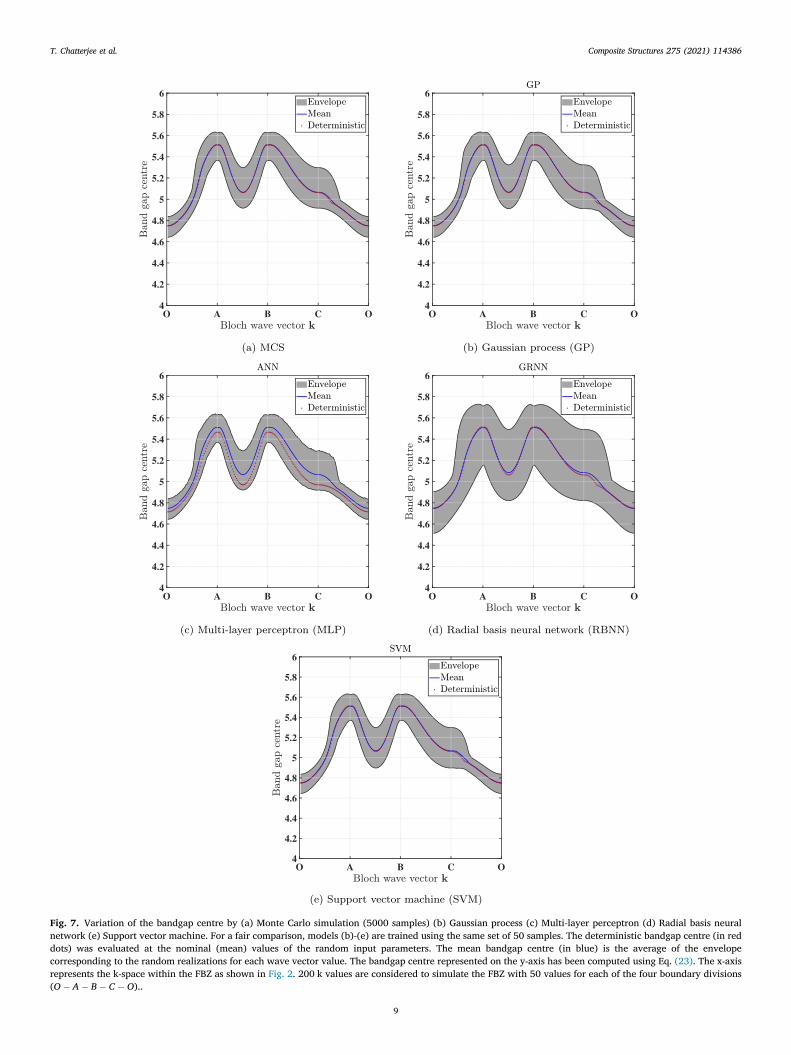
Fig. 7. Variation of the bandgap centre by (a) Monte Carlo simulation (5000 samples) (b) Gaussian process (c) Multi-layer perceptron (d) Radial basis neuralnetwork (e) Support vector machine. For a fair comparison, models (b)-(e) are trained using the same set of 50 samples. The deterministic bandgap centre (in reddots) was evaluated at the nominal (mean) values of the random input parameters. The mean bandgap centre (in blue) is the average of the envelopecorresponding to the random realizations for each wave vector value. The bandgap centre represented on the y-axis has been computed using Eq. (23). The x-axisrepresents the k-space within the FBZ as shown in Fig. 2. 200 k values are considered to simulate the FBZ with 50 values for each of the four boundary divisions(O� A� B� C � O)..

T. Chatterjee et al. Composite Structures 275 (2021) 114386

9

Fig. 8. Probability density functions at various positions of irreducible Brillouin zone (a) O (b) A (c) B (d) C.

T. Chatterjee et al. Composite Structures 275 (2021) 114386

Note that the bandgap has been indicated by a light yellow band inFig. 6. The variation in the bandgap centre position and relative fre-quency of the bandgap have been studied in Figs. 7 and 9, respectively.Since the difference of the variation of bandgap centres is not clearfrom Fig. 7, the probability density functions (PDF) of the bandgapcentres at the four points of IRBZ (refer Fig. 2) obtained by the MLtechniques are presented in Fig. 8. It can be observed from the resultsthat all the ML techniques have performed well in capturing the over-all variation in the centre position and relative frequency of the band-gap. Only the approximation of bandgap centre by RBNN in Fig. 7d isrelatively poor (also evident from Fig. 8d). Although the mean of thebandgap centre is well estimated, the extremum points are slightlyoverestimated. This can be improved either by tuning some of the net-work parameters or increasing the number of training samples. Havingsaid this, the performance of RBNN is not even close to being unac-ceptable considering significantly fewer models are employed forRBNN compared to GP and SVM. Note that instead of the above MLtechniques, any other approaches can be easily fused in the abovenon‐intrusive stochastic framework, provided it is capable of capturingthe highly sensitive non‐linear wave response variation.

10

4.2. Analysis at the global structural level

To verify the results of the above frequency band structuresobtained by considering the Bloch theorem and unit cell, frequencyresponse functions (FRF) corresponding to a rectangular plate‐likestructure for clamped‐free‐free‐free (CFFF) boundary conditions, asshown in Fig. 10, have been determined.

The stochastic dynamic response of the structural system consid-ered in Fig. 10 has been investigated. The length and width of thefinite dimension honeycomb lattice structure are related to the lengthof the beam segment L and lattice angle θ. The input uncertainty hasbeen assumed at the unit cell level and is same as that of the stochasticwave propagation analysis performed above (refer Table 1). This anal-ysis is intended towards quantifying the effect of micro‐structuralanomalies on the global dynamic behaviour of the structural system.The input uncertainty in the form of material and geometric parame-ters at the unit cell level of the lattice system is propagated to the glo-bal mass and stiffness matrices, and a stochastic eigenvalue problem isposed taking into account the global random system matrices (com-prising 3420 DOFs) for the undamped case. Corresponding to a ran-

Fig. 9. Variation of the relative frequency of bandgap by (a) Monte Carlo simulation (5000 samples) (b) Gaussian process (c) Multi-layer perceptron (d) Radialbasis neural network (e) Support vector machine. For a fair comparison, models (b)-(e) are trained using the same set of 50 samples. The deterministic relativefrequency of bandgap (in red dots) was evaluated at the nominal (mean) values of the random input parameters. The mean relative frequency (in blue) is theaverage of the envelope corresponding to the random realizations for each wave vector value. The bandgap relative frequency represented on the y-axis has beencomputed using Eq. (24). The x-axis represents the k-space within the FBZ as shown in Fig. 2. 200 k values are considered to simulate the FBZ with 50 values foreach of the four boundary divisions (O� A� B� C � O)..

T. Chatterjee et al. Composite Structures 275 (2021) 114386

11

Fig. 10. The finite dimensional lattice honeycomb structure with clamped-free-free-free boundary conditions. The blue color marked points represent thefixed points of clamped boundary condition.

T. Chatterjee et al. Composite Structures 275 (2021) 114386

dom realization of the modal solutions, FRFs are obtained. For valida-tion of the location of the bandgap at the unit cell and global structurallevel, the undamped deterministic dispersion curve and deterministicFRF with negligible damping (0.01 %) have been compared inFigs. 11a and 11b, respectively. The band plot of FRF considering ran-dom input parameters has been presented in Fig. 11c. Fig. 11 illus-trates that the position of the bandgap at the unit cell and globalstructural level is the same, which validates the model.

Next, the performance of the ML techniques has been assessed inthe context of their approximation capability of the frequencyresponse at the global structural level. For this, each of the modal solu-tions is represented by individual ML techniques. Corresponding to a

Fig. 11. Validation of the bandgap at the (a) unit cell level (deterministic) (b)Frequency response functions in (b) and (c) are obtained corresponding to 0.01%

12

random realization of the modal solutions, FRFs are obtained consider-ing 0.5% damping. Consequently, the propagation of the input uncer-tainty to the dynamic response using the ML techniques only require anominal number of analytical or FE simulations of the actual system.The computational efficiency achieved by ML has been quantifiedlater. For training the ML models, the same set of 50 training samplesare employed as selected previously from the convergence study inFig. 5. The configuration of the ML models is also the same as above.For validation, 1000 samples of MCS (test data set) are used. The vari-ation of the FRFs are presented in Figs. 12 and 13.

Sample direct and cross FRF band plots corresponding to the DOFsof edge nodes are presented in Figs. 12 and 13, respectively. Specifi-cally nodes at the edges have been selected for demonstration as itwould be convenient to experimentally measure the FRFs at these loca-tions from a practical point of view. Note that the bandgaps are notidentifiable from the sample FRF plots in Figs. 12 and 13 as the band-gaps are essentially obtained from undamped eigenvalue analysiswhereas the FRFs are evaluated considering 0.5 % damping. Thehigher damping (compared to 0.01 % damping in Fig. 11c) averagesout the frequency response as evident from the ensemble mean FRFswhich makes the bandgap disappear. In general, it can be observedfrom Figs. 12 and 13 that close proximity has been achieved betweenthe ML (approximate) and MCS (actual) based stochastic frequencyresponse. It can be visually observed that the performance of RBNNin capturing the overall response variation is not as robust as the otherML techniques used. This can possibly be improved either by tuningsome of the network parameters or increasing the number of trainingsamples. For an explicit assessment of the approximation accuracyachieved by the ML models, the RMSE of the mean and standard devi-ation of the FRFs are presented in Table 2.

To analyze the global structure comprising 3420 DOFs, significantcomputational savings was achieved by the ML models, which is quan-tified next. The time required to perform a single eigenvalue analysistook around 480 s on an Intel® Xeon® W‐2145 CPU @ 3.70 GHz,3696 MHz, with 8 cores and 16 logical processors. Hence, the timerequired for 1000 MCS samples was (1000 � 480) s, equivalent to5.56 days. The time required to generate samples for the ML modelswas (50 � 480) s, equivalent to 6.67 h. The model building timerequired by GP, ANN, RBNN and SVM was calculated to be 4.34 s,401.38 s, 61.81 s and 18.39 s, respectively. Consequently, the ML mod-els required 5–5.1 % CPU time compared to MCS for solving thestochastic problem. Thus, from these results, it is reasonable to infer

global structural level (deterministic) (c) global structural level (stochastic).damping. (c) is obtained by 1000 Monte Carlo simulations.

Fig. 12. Sample direct frequency response function H(1,1) band plots (a) Monte Carlo simulation (1000 samples) (b) Gaussian process (c) Multi-layer perceptron(d) Radial basis neural network (e) Support vector machine. For a fair comparison, models (b)-(e) are trained using the same set of 50 samples. The grey enveloperepresents the maximum/minimum points. The green envelope represents the 95% confidence interval points. The deterministic frequency response function (inred) was evaluated at the nominal (mean) values of the random input parameters. The ensemble mean frequency response function (in blue) is the average of theenvelope corresponding to the random realizations for each forcing frequency value.

T. Chatterjee et al. Composite Structures 275 (2021) 114386

13

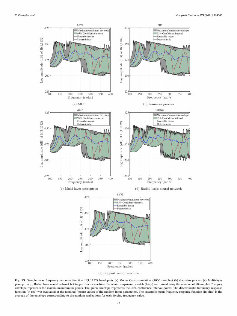
Fig. 13. Sample cross frequency response function H(1,1132) band plots (a) Monte Carlo simulation (1000 samples) (b) Gaussian process (c) Multi-layerperceptron (d) Radial basis neural network (e) Support vector machine. For a fair comparison, models (b)-(e) are trained using the same set of 50 samples. The greyenvelope represents the maximum/minimum points. The green envelope represents the 95% confidence interval points. The deterministic frequency responsefunction (in red) was evaluated at the nominal (mean) values of the random input parameters. The ensemble mean frequency response function (in blue) is theaverage of the envelope corresponding to the random realizations for each forcing frequency value.

T. Chatterjee et al. Composite Structures 275 (2021) 114386

14

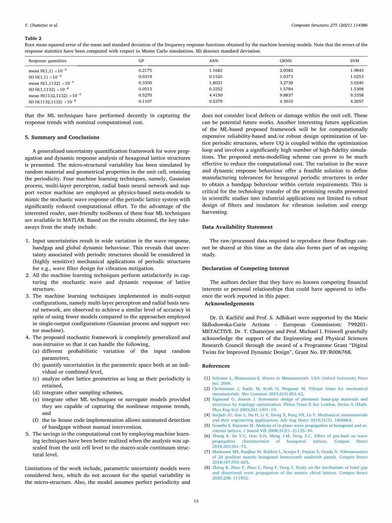
Table 2Root mean squared error of the mean and standard deviation of the frequency response functions obtained by the machine learning models. Note that the errors of theresponse statistics have been computed with respect to Monte Carlo simulations. SD denotes standard deviation.

Response quantities GP ANN GRNN SVM

mean H(1,1) �10�9 0.2175 1.1682 2.0582 1.9843

SD H(1,1) �10�8 0.0319 0.1525 1.0373 1.0253

mean H(1,1132) �10�9 0.3350 1.8021 3.2730 3.0245

SD H(1,1132) �10�8 0.0513 0.2252 1.5784 1.5308

mean H(1132,1132) �10�9 0.5270 4.4150 9.8837 9.3358

SD H(1132,1132) �10�8 0.1107 0.5370 4.3010 4.2057

T. Chatterjee et al. Composite Structures 275 (2021) 114386

that the ML techniques have performed decently in capturing theresponse trends with nominal computational cost.

5. Summary and Conclusions

A generalized uncertainty quantification framework for wave prop-agation and dynamic response analysis of hexagonal lattice structuresis presented. The micro‐structural variability has been simulated byrandom material and geometrical properties in the unit cell, retainingthe periodicity. Four machine learning techniques, namely, Gaussianprocess, multi‐layer perceptron, radial basis neural network and sup-port vector machine are employed as physics‐based meta‐models tomimic the stochastic wave response of the periodic lattice system withsignificantly reduced computational effort. To the advantage of theinterested reader, user‐friendly toolboxes of these four ML techniquesare available in MATLAB. Based on the results obtained, the key take‐aways from the study include:

1. Input uncertainties result in wide variation in the wave response,bandgap and global dynamic behaviour. This reveals that uncer-tainty associated with periodic structures should be considered in(highly sensitive) mechanical applications of periodic structuresfor e.g., wave filter design for vibration mitigation.

2. All the machine learning techniques perform satisfactorily in cap-turing the stochastic wave and dynamic response of latticestructure.

3. The machine learning techniques implemented in multi‐outputconfigurations, namely multi‐layer perceptron and radial basis neu-ral network, are observed to achieve a similar level of accuracy inspite of using fewer models compared to the approaches employedin single‐output configurations (Gaussian process and support vec-tor machine).

4. The proposed stochastic framework is completely generalized andnon‐intrusive so that it can handle the following,(a) different probabilistic variation of the input random

parameters,(b) quantify uncertainties in the parametric space both at an indi-

vidual or combined level,(c) analyze other lattice geometries as long as their periodicity is

retained,(d) integrate other sampling schemes,(e) integrate other ML techniques or surrogate models provided

they are capable of capturing the nonlinear response trends,and

(f) the in–house code implementation allows automated detectionof bandgaps without manual intervention.

5. The savings in the computational cost by employing machine learn-ing techniques have been better realized when the analysis was up‐scaled from the unit cell level to the macro‐scale continuum struc-tural level.

Limitations of the work include, parametric uncertainty models wereconsidered here, which do not account for the spatial variability inthe micro‐structure. Also, the model assumes perfect periodicity and

15

does not consider local defects or damage within the unit cell. Thesecan be potential future works. Another interesting future applicationof the ML‐based proposed framework will be for computationallyexpensive reliability‐based and/or robust design optimization of lat-tice periodic structures, where UQ is coupled within the optimizationloop and involves a significantly high number of high‐fidelity simula-tions. The proposed meta‐modelling scheme can prove to be mucheffective to reduce the computational cost. The variation in the waveand dynamic response behaviour offer a feasible solution to definemanufacturing tolerances for hexagonal periodic structures in orderto obtain a bandgap behaviour within certain requirements. This iscritical for the technology transfer of the promising results presentedin scientific studies into industrial applications not limited to robustdesign of filters and insulators for vibration isolation and energyharvesting.

Data Availability Statement

The raw/processed data required to reproduce these findings can-not be shared at this time as the data also forms part of an ongoingstudy.

Declaration of Competing Interest

The authors declare that they have no known competing financialinterests or personal relationships that could have appeared to influ-ence the work reported in this paper.Acknowledgements

Dr. D. Karličić and Prof. S. Adhikari were supported by the MarieSkłlodowska‐Curie Actions ‐ European Commission: 799201‐METACTIVE. Dr. T. Chatterjee and Prof. Michael I. Friswell gratefullyacknowledge the support of the Engineering and Physical SciencesResearch Council through the award of a Programme Grant “DigitalTwins for Improved Dynamic Design”, Grant No. EP/R006768.

References

[1] Solymar L, Shamonina E. Waves in Metamaterials. USA: Oxford University PressInc; 2009.

[2] Christensen J, Kadic M, Kraft O, Wegener M. Vibrant times for mechanicalmetamaterials. Mrs Commun 2015;5(3):453–62.

[3] Sigmund O, Jensen J. Systematic design of phononic band-gap materials andstructures by topology optimization. Philos Trans R Soc London, Series A (Math,Phys Eng Sci) 2003;361:1001–19.

[4] Surjadi JU, Gao L, Du H, Li X, Xiong X, Fang NX, Lu Y. Mechanical metamaterialsand their engineering applications. Adv Eng Mater 2019;21(3). 1800864.

[5] Gonella S, Ruzzene M. Analysis of in-plane wave propagation in hexagonal and re-entrant lattices. J Sound Vib 2008;312(1–2):125–39.

[6] Zhang K, Su Y-C, Hou X-H, Meng J-M, Deng Z-C. Effect of pre-load on wavepropagation characteristics of hexagonal lattices. Compos Struct2018;203:361–72.

[7] Mazloomi MS, Ranjbar M, Boldrin L, Scarpa F, Patsias S, Ozada N. Vibroacousticsof 2d gradient auxetic hexagonal honeycomb sandwich panels. Compos Struct2018;187:593–603.

[8] Zhang K, Zhao P, Zhao C, Hong F, Deng Z. Study on the mechanism of band gapand directional wave propagation of the auxetic chiral lattices. Compos Struct2020;238: 111952.

T. Chatterjee et al. Composite Structures 275 (2021) 114386

[9] Karličić D, Cajić M, Chatterjee T, Adhikari S. Wave propagation in mass embeddedand pre-stressed hexagonal lattices. Compos Struct 2021;256: 113087.

[10] Iwata Y, Yokozeki T. Shock wave filtering of two-dimensional cfrp x-latticestructures: A numerical investigation. Compos Struct 2021;265: 113743.

[11] Iwata Y, Yokozeki T. Wave propagation analysis of one-dimensional cfrp latticestructure. Compos Struct 2021;261: 113306.

[12] Xiao X, He Z, Li E, Zhou B, Li X. A lightweight adaptive hybrid laminatemetamaterial with higher design freedom for wave attenuation. Compos Struct2020;243: 112230.

[13] Li J, Yang P, Li S. Phononic band gaps by inertial amplification mechanisms inperiodic composite sandwich beam with lattice truss cores. Compos Struct2020;231: 111458.

[14] Gasparetto VE, ElSayed MS. Multiscale optimization of specific elastic propertiesand microscopic frequency band-gaps of architectured microtruss lattice materials.Int J Mech Sci 2021;197: 106320.

[15] Ayad M, Karathanasopoulos N, Reda H, Ganghoffer J, Lakiss H. Dispersioncharacteristics of periodic structural systems using higher order beam elementdynamics. Math Mech Solids 2020;25(2):457–74.

[16] Reda H, Karathanasopoulos N, Ganghoffer J, Lakiss H. Wave propagationcharacteristics of periodic structures accounting for the effect of their higherorder inner material kinematics. J Sound Vib 2018;431:265–75.

[17] Reda H, Rahali Y, Ganghoffer J, Lakiss H. Wave propagation analysis in 2dnonlinear hexagonal periodic networks based on second order gradient nonlinearconstitutive models. Int J Non-Linear Mech 2016;87:85–96.

[18] Karathanasopoulos N, Reda H, Ganghoffer J. The role of non-slender innerstructural designs on the linear and non-linear wave propagation attributes ofperiodic, two-dimensional architectured materials. J Sound Vib 2019;455:312–23.

[19] Pal RK, Ruzzene M, Rimoli JJ. Tunable wave propagation by varying prestrain intensegrity-based periodic media. Extreme Mech Lett 2018;22:149–56.

[20] Pajunen K, Celli P, Daraio C. Prestrain-induced bandgap tuning in 3d-printedtensegrity-inspired lattice structures. Extreme Mech Lett 2021;44: 101236.

[21] Liu K, Zegard T, Pratapa PP, Paulino GH. Unraveling tensegrity tessellations formetamaterials with tunable stiffness and bandgaps. J Mech Phys Solids2019;131:147–66.

[22] Celli P, Gonella S, Tajeddini V, Muliana A, Ahmed S, Ounaies Z. Wave controlthrough soft microstructural curling: bandgap shifting, reconfigurable anisotropyand switchable chirality. Smart Mater Struct 2017;26(3): 035001.

[23] Nimmagadda C, Matlack KH. Thermally tunable band gaps in architectedmetamaterial structures. J Sound Vib 2019;439:29–42.

[24] Wu Y, Lin XY, Jiang HX, Cheng AG. Finite element analysis of the uncertainty ofphysical response of acoustic metamaterials with interval parameters. Int JComput Methods 2020;17(08):1950052.

[25] Schevenels M, Lazarov B, Sigmund O. Robust topology optimization accounting forspatially varying manufacturing errors. Comput Methods Appl Mech Eng 2011;200(49):3613–27.

[26] Celli P, Yousefzadeh B, Daraio C, Gonella S. Bandgap widening by disorder inrainbow metamaterials. Appl Phys Lett 2019;114: 091903.

[27] Henneberg J, Gomez Nieto JS, Sepahvand K, Gerlach A, Cebulla H, Marburg S.Periodically arranged acoustic metamaterial in industrial applications: The needfor uncertainty quantification. Appl Acoust 2020;157: 107026.

[28] Wagner P-R, Dertimanis VK, Chatzi EN, Beck JL. Robust-to-uncertainties optimaldesign of seismic metamaterials. J Eng Mech 2018;144(3):04017181.

[29] Chuang K-C, Zhang Z-Q, Wang H-X. Experimental study on slow flexural wavesaround the defect modes in a phononic crystal beam using fiber bragg gratings.Phys Lett A 2016;380(47):3963–9.

[30] Yao Z-J, Yu G-L, Wang Y-S, Shi Z-F. Propagation of bending waves in phononiccrystal thin plates with a point defect. Int J Solids Struct 2009;46(13):2571–6.

[31] Mencik J-M, Duhamel D. A wave finite element-based approach for the modelingof periodic structures with local perturbations. Finite Elem Anal Des2016;121:40–51.

[32] Do XN, Reda H, Ganghoffer JF. Impact of damage on the effective properties ofnetwork materials and on bulk and surface wave propagation characteristics.Continuum Mech Thermodyn 2021;33(2):369–401.

[33] Reda H, Rahali Y, Vieille B, Lakiss H, Ganghoffer J. Impact of damage on thepropagation of rayleigh waves in lattice materials. Int J Damage Mech 2021;30(5):665–80.

[34] Dey S, Mukhopadhyay T, Adhikari S. Uncertainty Quantification in LaminatedComposites: A Meta-model Based Approach. Boca Raton, FL, USA: Taylor & FrancisInc (CRC Press); 2018.

[35] Babaa HA, Nandi S, Singh T, Nouh M. Uncertainty Quantification of TunableElastic Metamaterials using Polynomial Chaos. J Appl Phys 2020;127: 015102.

[36] Chatterjee T, Karličić D, Adhikari S, Friswell MI. Gaussian process assistedstochastic dynamic analysis with applications to near-periodic structures. MechSyst Signal Processing 2021;149: 107218.

16

[37] He ZC, Hu JY, Li E. An uncertainty model of acoustic metamaterials with randomparameters. Comput Mech 2018;62:1023–36.

[38] Beli D, Fabro A, Ruzzene M, Arruda JRF. Wave attenuation and trapping in 3dprinted cantilever-in-mass metamaterials with spatially correlated variability. SciRep 2019;9:5617.

[39] Fabro AT, Meng H, Chronopoulos D. Uncertainties in the attenuation performanceof a multi-frequency metastructure from additive manufacturing. Mech Syst SignalProcessing 2020;138: 106557.

[40] Finol D, Lu Y, Mahadevan V, Srivastava A. Deep convolutional neural networks foreigenvalue problems in mechanics. Int J Numer Meth Eng 2019;118(5):258–75.

[41] Bacigalupo A, Gnecco G, Lepidi M, Gambarotta L. Machine-learning techniques forthe optimal design of acoustic metamaterials. J Optim Theory Appl 2020;187(3):630–53.

[42] Bloch F. Quantum mechanics of electrons in crystal lattices. Z Phys1928;52:555–600.

[43] Hussein MI, Leamy MJ, Ruzzene M. Dynamics of phononic materials andstructures: Historical origins, recent progress, and future outlook. Appl MechRev 2014;66(4): 040802.

[44] Collet M, Ouisse M, Ruzzene M, Ichchou M. Floquet–bloch decomposition for thecomputation of dispersion of two-dimensional periodic, damped mechanicalsystems. Int J Solids Struct 2011;48(20):2837–48.

[45] Leamy MJ. Exact wave-based bloch analysis procedure for investigating wavepropagation in two-dimensional periodic lattices. J Sound Vib 2012;331(7):1580–96.

[46] Kittel C, McEuen P, McEuen P. Introduction to Solid State Physics, Vol. 8. NewYork: Wiley; 1996.

[47] Meng J, Deng Z, Zhang K, Xu X. Wave propagation in hexagonal and re-entrantlattice structures with cell walls of non-uniform thickness. Waves RandomComplex Media 2015;25(2):223–42.

[48] Scheidt JV, Purkert W. Random Eigenvalue Problems. New York: North Holland;1983.

[49] Adhikari S. Joint statistics of natural frequencies of stochastic dynamic systems.Comput Mech 2007;40(4):739–52.

[50] Krige DG. A Statistical approach to some basic mine valuation problems on thewitwatersrand. J Chem, Metall Mining Society South Africa 1951;52(6):119–39.

[51] DiazDelaO FA, Adhikari S. Structural dynamic analysis using gaussian processemulators. Eng Comput 2010;27(5):580–605.

[52] Chatterjee T, Adhikari S, Friswell MI. Uncertainty propagation in dynamic sub-structuring by model reduction integrated domain decomposition. ComputMethods Appl Mech Eng 2020;366: 113060.

[53] DiazDelaO FA, Adhikari S. Gaussian process emulators for the stochastic finiteelement method. Int J Numer Methods Eng 2011;87(6):521–40.

[54] Chatterjee T, Chowdhury R. Adaptive Bilevel Approximation Technique forMultiobjective Evolutionary Optimization. J Computing Civil Eng 2017;31(3):04016071.

[55] Chatterjee T, Chowdhury R, Ramu P. Decoupling Uncertainty Quantification fromRobust Design Optimization. Struct Multidisciplinary Optimization2019;59:1969–90.

[56] Rasmussen CE, Williams CKI. Gaussian Processes for MachineLearning. Cambridge, Massachusetts London, England: The MIT Press; 2006.

[57] Lophaven S, Nielson H, Sondergaard J, DACE A MATLAB Kriging Toolbox, Tech.rep., Technical University of Denmark, IMM-TR-2002-12, Technical University ofDenmark; 2002. .

[58] Moustapha M, Bourinet JM, Guillaume B, Sudret B. Comparative Study of Krigingand Support Vector Regression for Structural Engineering Applications. JUncertainty Eng Syst, Part A: Civil Eng 2018;4(2):04018005.

[59] Chatterjee T, Chowdhury R. h – p adaptive model based approximation of momentfree sensitivity indices. Comput Methods Appl Mech Eng 2018;332:572–99.

[60] Goodfellow I, Bengio Y, Courville A. Deep learning. MIT press 2016.[61] Hecht-Nielsen R. Applications of counterpropagation networks. Neural Networks

1988;1(2):131–9.[62] Rumelhart DE, Hinton GE, Williams RJ. Learning representations by back-

propagating errors. Nature 1986;323:533–6.[63] Cortes C, Vapnik V. Support-vector networks. Mach Learn 1995;20(3):273–97.[64] Boser BE, Guyon IM, Vapnik VN. A training algorithm for optimal margin

classifiers. In: Proceedings of the fifth annual workshop on Computational learningtheory. p. 144–52.

[65] Vapnik V, Lerner A. Generalized portrait method for pattern recognition.Automation Remote Control 1963;24(6):774–80.

[66] McKay M, Beckman RJ, Conover WJ. A comparison of three methods for selectingvalues of input variables in the analysis of output from a computer code.Technometrics 1979;21(2):239–45.