wave dark matter and dwarf spheroidal galaxies - department of
TRANSCRIPT

Wave Dark Matter and Dwarf Spheroidal Galaxies
by
Alan R. Parry
Department of MathematicsDuke University
Date:Approved:
Hubert L. Bray, Supervisor
Paul S. Aspinwall
Arlie O. Petters
Thomas P. Witelski
Dissertation submitted in partial fulfillment of the requirements for the degree ofDoctor of Philosophy in the Department of Mathematics
in the Graduate School of Duke University2013

Abstract
Wave Dark Matter and Dwarf Spheroidal Galaxies
by
Alan R. Parry
Department of MathematicsDuke University
Date:Approved:
Hubert L. Bray, Supervisor
Paul S. Aspinwall
Arlie O. Petters
Thomas P. Witelski
An abstract of a dissertation submitted in partial fulfillment of the requirements forthe degree of Doctor of Philosophy in the Department of Mathematics
in the Graduate School of Duke University2013

Copyright c© 2013 by Alan R. ParryAll rights reserved except the rights granted by the
Creative Commons Attribution-Noncommercial Licence

Abstract
We explore a model of dark matter called wave dark matter (also known as scalar field
dark matter and boson stars) which has recently been motivated by a new geometric
perspective by Bray (Bray (2010)). Wave dark matter describes dark matter as a
scalar field which satisfies the Einstein-Klein-Gordon equations. These equations
rely on a fundamental constant Υ (also known as the “mass term” of the Klein-
Gordon equation). Specifically, in this dissertation, we study spherically symmetric
wave dark matter and compare these results with observations of dwarf spheroidal
galaxies as a first attempt to compare the implications of the theory of wave dark
matter with actual observations of dark matter. This includes finding a first estimate
of the fundamental constant Υ.
In the introductory Chapter 1, we present some preliminary background material
to define and motivate the study of wave dark matter and describe some of the
properties of dwarf spheroidal galaxies.
In Chapter 2, we present several different ways of describing a spherically sym-
metric spacetime and the resulting metrics. We then focus our discussion on an es-
pecially useful form of the metric of a spherically symmetric spacetime in polar-areal
coordinates and its properties. In particular, we show how the metric component
functions chosen are extremely compatible with notions in Newtonian mechanics.
We also show the monotonicity of the Hawking mass in these coordinates. Finally,
we discuss how these coordinates and the metric can be used to solve the spherically
iv

symmetric Einstein-Klein-Gordon equations.
In Chapter 3, we explore spherically symmetric solutions to the Einstein-Klein-
Gordon equations, the defining equations of wave dark matter, where the scalar field
is of the form fpt, rq eiωtF prq for some constant ω P R and complex-valued function
F prq. We show that the corresponding metric is static if and only if F prq hprqeia
for some constant a P R and real-valued function hprq. We describe the behavior of
the resulting solutions, which are called spherically symmetric static states of wave
dark matter. We also describe how, in the low field limit, the parameters defining
these static states are related and show that these relationships imply important
properties of the static states.
In Chapter 4, we compare the wave dark matter model to observations to obtain
a working value of Υ. Specifically, we compare the mass profiles of spherically sym-
metric static states of wave dark matter to the Burkert mass profiles that have been
shown by Salucci et al. (Salucci et al. (2012)) to predict well the velocity dispersion
profiles of the eight classical dwarf spheroidal galaxies. We show that a reason-
able working value for the fundamental constant in the wave dark matter model is
Υ 50 yr1. We also show that under precise assumptions the value of Υ can be
bounded above by 1000 yr1.
In order to study non-static solutions of the spherically symmetric Einstein-Klein-
Gordon equations, we need to be able to evolve these equations through time numer-
ically. Chapter 5 is concerned with presenting the numerical scheme we will use to
solve the spherically symmetric Einstein-Klein-Gordon equations in our future work.
We will discuss how to appropriately implement the boundary conditions into the
scheme as well as some artificial dissipation. We will also discuss the accuracy and
stability of the scheme. Finally, we will present some examples that show the scheme
in action.
In Chapter 6, we summarize our results. Finally, Appendix A contains a deriva-
v

tion of the Einstein-Klein-Gordon equations from its corresponding action.
vi

This dissertation is dedicated to my wife and children.
vii

Contents
Abstract iv
List of Tables xi
List of Figures xii
List of Abbreviations and Symbols xvii
Acknowledgements xx
1 Introduction 1
1.1 Basic Ideas of General Relativity . . . . . . . . . . . . . . . . . . . . 2
1.2 Dark Matter . . . . . . . . . . . . . . . . . . . . . . . . . . . . . . . . 6
1.3 Axioms of General Relativity . . . . . . . . . . . . . . . . . . . . . . 10
1.4 Wave Dark Matter . . . . . . . . . . . . . . . . . . . . . . . . . . . . 14
1.5 Dwarf Spheroidal Galaxies . . . . . . . . . . . . . . . . . . . . . . . . 15
2 A Survey of Spherically Symmetric Spacetimes 18
2.1 Metrics for a Spherically Symmetric spacetime . . . . . . . . . . . . . 19
2.2 A Newtonian-Compatible Metric . . . . . . . . . . . . . . . . . . . . 27
2.2.1 Compatibility with Newtonian Physics . . . . . . . . . . . . . 28
2.2.2 Other Useful Properties of this Metric . . . . . . . . . . . . . 34
2.3 The Einstein-Klein-Gordon Equations . . . . . . . . . . . . . . . . . . 36
2.4 Proofs . . . . . . . . . . . . . . . . . . . . . . . . . . . . . . . . . . . 41
viii

3 Spherically Symmetric Static Statesof Wave Dark Matter 75
3.1 The Spherically Symmetric Einstein-Klein-Gordon Equations . . . . . 76
3.2 Spherically Symmetric Static States . . . . . . . . . . . . . . . . . . . 79
3.2.1 ODEs for Static States . . . . . . . . . . . . . . . . . . . . . . 82
3.2.2 Boundary Conditions . . . . . . . . . . . . . . . . . . . . . . . 84
3.2.3 Plots of Static States . . . . . . . . . . . . . . . . . . . . . . . 92
3.3 Families of Static States . . . . . . . . . . . . . . . . . . . . . . . . . 92
3.3.1 Scalings of Static States . . . . . . . . . . . . . . . . . . . . . 98
3.3.2 Properties of Static State Mass Profiles . . . . . . . . . . . . . 102
3.4 Conclusion . . . . . . . . . . . . . . . . . . . . . . . . . . . . . . . . . 105
4 Modeling Wave Dark Matterin Dwarf Spheroidal Galaxies 107
4.1 Burkert Mass Profiles . . . . . . . . . . . . . . . . . . . . . . . . . . . 108
4.2 Static States of Wave Dark Matter . . . . . . . . . . . . . . . . . . . 112
4.2.1 Fitting Burkert Mass Profiles . . . . . . . . . . . . . . . . . . 114
4.2.2 Working Value of Υ . . . . . . . . . . . . . . . . . . . . . . . . 115
4.2.3 Upper Bound for Υ . . . . . . . . . . . . . . . . . . . . . . . . 116
4.2.4 Lower Bound for Υ . . . . . . . . . . . . . . . . . . . . . . . . 121
4.3 Utilized Approximations . . . . . . . . . . . . . . . . . . . . . . . . . 123
4.4 Conclusions . . . . . . . . . . . . . . . . . . . . . . . . . . . . . . . . 124
5 A Numerical Scheme to Solve theEinstein-Klein-Gordon Equationsin Spherical Symmetry 126
5.1 The Numerical Scheme . . . . . . . . . . . . . . . . . . . . . . . . . . 131
5.2 Stability and Accuracy of the Scheme . . . . . . . . . . . . . . . . . . 148
5.2.1 Stability of the Scheme . . . . . . . . . . . . . . . . . . . . . . 149
ix
5.2.2 Accuracy of the Scheme . . . . . . . . . . . . . . . . . . . . . 150
5.3 Explanation of the Matlab Code . . . . . . . . . . . . . . . . . . . . . 150
5.3.1 Examples . . . . . . . . . . . . . . . . . . . . . . . . . . . . . 152
6 Conclusions 157
A The Derivation of theEinstein-Klein-Gordon Equations 159
A.1 Varying the Metric . . . . . . . . . . . . . . . . . . . . . . . . . . . . 160
A.2 Varying the Scalar Field . . . . . . . . . . . . . . . . . . . . . . . . . 163
A.3 The Einstein-Klein-Gordon Equations . . . . . . . . . . . . . . . . . . 164
Bibliography 165
Biography 172
x

List of Tables
3.1 Values of the constants in the system (3.62) for the ground throughfifth excited states as well as the tenth and twentieth excited states.We have given them error ranges which encompass the interval we ob-served in our experiments. However, it is possible that values outsideour ranges here could be observed, though we don’t expect them tobe so by much if the discretization of r used in solving the ODEs issufficiently fine. Note also that our values have less precision as weincrease n. This is because as n increases, it becomes more difficultto compute the states with as much precision. . . . . . . . . . . . . . 97
4.1 Burkert mass profile data for the eight classical dwarf spheroidal galax-ies converted to units of years for mass, length, and time. The param-eters ρ0 and rc are those found by Salucci et al. for the best fit Burkertprofiles (Salucci et al. (2012)), and rlast is the radius of the outermostdata point given by Walker et al. (Walker et al. (2009, 2010)). Alsoincluded is the value of the inflection point, rip, of the Burkert massprofile for each galaxy and the ratio of rlast to rip. . . . . . . . . . . . 114
4.2 Upper bound values for Υ corresponding to poor best fits of the Burk-ert mass profiles for each of the classic dwarf spheroidal galaxies. Thevalues in each column for each galaxy should be interpreted as an up-per bound on the value of Υ, under the approximations explained inthe paper, if that galaxy is best modeled by an nth excited state. Theunits on Υ are yr1. . . . . . . . . . . . . . . . . . . . . . . . . . . . 121
xi

List of Figures
1.1 The light cone in Minkowski space projected into the pt, xq plane. Atimelike, spacelike, and lightlike or null vector is depicted in the figure. 3
1.2 The earth traveling along a geodesic in the curved spacetime generatedby the sun. Image credit: http://einstein.stanford.edu/. . . . . . . . . 5
1.3 The rotation curves, both observed and calculated, for the Andromedagalaxy. Credit: Queens University. . . . . . . . . . . . . . . . . . . . 7
1.4 The Bullet Cluster. The pink clouds are where the visible matterfrom the galaxy clusters is located, while the blue represents thedark matter. Credit: NASA/CXC/CfA/M.Markevitch et al.; Opti-cal: NASA/STScI; Magellan/U.Arizona/D.Clowe et al.; Lensing Map:NASA/STScI; ESO WFI; Magellan/U.Arizona/D.Clowe et al. . . . . 8
1.5 Fornax Dwarf Spheroidal Galaxy. Photo Credit: ESO/Digital SkySurvey 2 . . . . . . . . . . . . . . . . . . . . . . . . . . . . . . . . . . 16
2.1 Infinitesimal distance in a t constant hypersurface foliated spacetime. 20
3.1 Plots of static state scalar fields (specifically the function F prq in(3.10)) in the ground state and first, second, and third excited states.Note the number of nodes (zeros) of each function. . . . . . . . . . . 93
3.2 Mass profiles for a static ground state and first, second, and thirdexcited states of wave dark matter. . . . . . . . . . . . . . . . . . . . 94
3.3 Energy density profiles for a static ground state and first, second, andthird excited states of wave dark matter. . . . . . . . . . . . . . . . . 95
3.4 Plots of the potential function, V , for a static ground state and first,second, and third excited states of wave dark matter. . . . . . . . . . 96
xii

3.5 Left: Log plot of the parameters ω and µ0 for a ground state andconstant value of Υ 5. The slope of this plot is almost exactly 12.We get the exact same slope for other values of Υ, thus ωpΥ, µ0q ΥeCfrequencypΥq
?µ0 . Right: Log plot of the parameters CfrequencypΥq and
Υ for a ground state. The slope of this plot is almost exactly 1. ThusCfrequencypΥq CfrequencyΥ, where Cfrequency is a constant. Similarplots exist for any nth excited state. . . . . . . . . . . . . . . . . . . . 97
3.6 Left: Plot of the mass profile of a ground state with its correspondinghyperbola of constant Υ overlayed. Any ground state mass profilethat keeps the presented relationship with this hyperbola correspondsto the same value of Υ. Right: Examples of different ground statemass profiles corresponding to the same value of Υ. The correspond-ing hyperbola of constant Υ is overlayed. Notice that all three massprofiles have the same relationship with the hyperbola. . . . . . . . . 103
3.7 Left: Plot of the mass profile of a ground state with its correspondinginitial cubic function overlayed. Right: Close up of the picture on theright in the region of small r. . . . . . . . . . . . . . . . . . . . . . . 104
4.1 Observed velocity dispersion profiles of the eight classical dwarf spher-oidal galaxies are denoted by the points on each plot with its associatederror bars. The solid lines overlayed on these profiles are the best fitvelocity dispersion profiles predicted by the Burkert mass profile. Thisfigure is directly reproduced from the paper by Salucci et al. (Salucciet al. (2012)) and the reader is referred to their paper for a completedescription of how these models were computed. . . . . . . . . . . . . 109
4.2 Plot of a Burkert mass profile. The inflection point is marked with an. . . . . . . . . . . . . . . . . . . . . . . . . . . . . . . . . . . . . . 110
4.3 Left: Plot of the Burkert mass profile for the Carina galaxy foundby Salucci et al. (Salucci et al. (2012)) along with a mass plot of awave dark matter static ground state, the cubic function which is theleading term of the Taylor expansion of the Burkert mass profile, and
the quadratic power functionMBprcqr2c
r2 where rc is the core radius of
the Carina galaxy. The marks the location of the inflection point ofthe Burkert mass profile, while the vertical line denotes the locationof the outermost data point for the Carina galaxy and is presented forreference purposes only. Right: Closeup of the plot on the left overthe r interval r0, rips. . . . . . . . . . . . . . . . . . . . . . . . . . . . 112
xiii

4.4 Plots of the Burkert mass profiles computed by Salucci et al. of theeight classical dwarf spheroidal galaxies within the range of observabledata. The inflection point is marked on each plot by an . Carina andDraco have no inflection point marked because the inflection point fortheir Burkert mass profiles occurs outside the range of observable data.113
4.5 Static state mass profiles for Υ 50 which are each a best fit to theBurkert profiles of the corresponding dwarf spheroidal galaxy. ForΥ 50, we picked an nth excited state whose best fit profile matchedthe Burkert profile qualitatively well. This shows that Υ 50 is areasonable working value of Υ. However, it does not imply that theactual value of Υ is 50 or that these galaxies are correctly modeled bythe presented nth excited state. The units on Υ are yr1. . . . . . . . 117
4.6 Left: Ground state mass profiles of various values of Υ that are bestfits to the Burkert mass profile found by Salucci et al. (Salucci et al.(2012)) for the Leo II galaxy. The corresponding hyperbolas of con-stant Υ on which these profiles lie are also plotted. Ground states andtheir corresponding hyperbolas are drawn in the same color. Right:The same plots as in the left frame, but with the constant functionwhich best fits the Burkert profile also plotted. Note that the best fitmass profiles approach this constant mass profile as Υ increases. . . . 118
4.7 The Burkert mass profile found by Salucci et al. (Salucci et al. (2012))for the Sextans galaxy. The best fit static state mass profiles for aground through fifth excited state, tenth excited state, and twentiethexcited state all lying on the same hyperbola are overlayed on theplot. The hyperbola here satisfies the rejection criteria for all of thedifferent static states represented in the plot, thus all of these staticstates correspond to an upper bound on the value of Υ for Sextansfor their respective value of n (i.e. the set of nth excited states). Notehow close together all of the states are. This is due to the fact thatthe majority of their profiles which are being compared to the Burkertmass profile is the common and constant portion of the profiles. . . . 120
4.8 The Burkert mass profile found by Salucci et al.Salucci et al. (2012)for the Leo II galaxy. The best fit ground state mass profiles forsuccessively smaller values of Υ are overlayed on the plot. Also plottedis the best fit cubic power function, ar3, which almost coincides withthe mass plot for Υ 1 and so is somewhat difficult to make out.However, it is apparent that for successively smaller values of Υ, thebest fit ground state approaches the best fit cubic function. . . . . . . 122
xiv

5.1 Image of an incoming and outgoing wave at the boundary rmax. Thefuture pointing outward null vector EO is also displayed. Since nooutgoing wave can travel faster than the speed of the null vector shown,then computing the change of f along this null vector will only detectchanges in f due to incoming waves. . . . . . . . . . . . . . . . . . . 129
5.2 Image of an incoming and outgoing wave at the boundary rmax. Thefuture pointing inward null vector EI is also displayed. Since no in-coming wave can travel faster than the speed of the null vector shown,then computing the change of f along this null vector will only detectchanges in f due to outgoing waves. . . . . . . . . . . . . . . . . . . . 129
5.3 A depiction of what is simulated by the boundary condition (5.2) withλ 1. In this case, all outgoing waves are replaced by incoming wavesof the same amplitude and phase. If we restrict our attention to theleft of the vertical dotted line representing r rmax, we see that thisis equivalent to the outgoing wave being immediately reflected by theboundary back into the system with the same amplitude and phase.All values of λ in the boundary condition (5.2) can be interpreted assome amplifying or damping phase-shifting reflection. . . . . . . . . . 130
5.4 A depiction of what is simulated by the boundary condition (5.2) withλ 1. In this case, all outgoing waves are replaced by incomingwaves of the same amplitude, but opposite phase (i.e. all peaks arevalleys and vice versa). If we restrict our attention to the left of thevertical dotted line representing r rmax, we see that this is equivalentto the outgoing wave being immediately reflected by the boundaryback into the system with the same amplitude, but opposite phase.All values of λ in the boundary condition (5.2) can be interpreted assome amplifying or damping phase-shifting reflection. . . . . . . . . . 131
xv
5.5 Output plot generated by the NCEKG program for a complex scalarfield. The upper left panel depicts the absolute value of the scalarfield, while the first two panels on the bottom row are plots of thereal and imaginary parts of the scalar field respectively. The secondand third upper panels are plots of the potential and mass functionsrespectively. The vertical dotted line in the plot of the potential tracesthe position of a particle in free fall in the system. The last two plotson the bottom row are plots of the energy density function µ and µtimes the surface area of a metric sphere of radius r. The upper rightpanel plots the difference between the current value of M at r rmaxthe initial value of M at r rmax as a function of t. This “mass lost”plot can be a visual measure of the error if the plot in question is notsupposed to lose mass, or it can serve as a visual representation of themass lost due to escaping waves. . . . . . . . . . . . . . . . . . . . . . 155
5.6 Output plot generated by the NCEKG program for a real scalar field.The upper left panel plots the scalar field. The second and third upperpanels are plots of the potential and mass functions respectively. Thevertical dotted line in the plot of the potential traces the position ofa particle in free fall in the system. The first two plots on the bottomrow are plots of the energy density function µ and µ times the surfacearea of a metric sphere of radius r. The lower right panel plots thedifference between the current value of M at r rmax the initial valueof M at r rmax as a function of t. This “mass lost” plot can be avisual measure of the error if the plot in question is not supposed tolose mass, or it can serve as a visual representation of the mass lostdue to escaping waves. . . . . . . . . . . . . . . . . . . . . . . . . . . 156
xvi

List of Abbreviations and Symbols
Symbols
This is a list of commonly used symbols in this dissertation. Unless otherwise noted
in the text, each symbol is defined as follows.
R The set of real numbers.
C The set of complex numbers.
e Euler’s number, e 2.71828....
i The imaginary unit.
Bx The coordinate vector fieldBBx corresponding to the coordinate
function x.
g The spacetime metric.
γ The induced metric of a submanifold of the spacetime, usuallythat of a spacelike hypersurface or a metric sphere.
∇ Used to denote a connection or covariant derivative. It will beclear from the context what it is.
Γ The Christoffel symbols of a connection.
R The Riemann curvature tensor.
Ric The Ricci curvature tensor.
R The scalar curvature.
G The Einstein curvature tensor, G Ric1
2Rg.
T The stress energy tensor.
xvii

Σ Usually a two-dimensional surface in a manifold.
Σt,r The metric sphere of radius r and time t.
mHpΣq The Hawking mass of the 2-dimensional surface Σ.
II The second fundamental form.
~H The mean curvature vector field.
H The Mean Curvature in Chapter 2 and the derivative of thefunction F prq otherwise.
Hf The Hessian of the function f .
2g The Laplacian operator on the spacetime with respect to themetric g.
t, r, θ, ϕ The names of the coordinates of a spherically symmetric space-time.
f The scalar field of the Einstein-Klein-Gordon equations.
p A multiple of the time derivative of f , defined specifically byequation (2.47).
V One of two of the metric functions in the spherically symmetricmetric in equation (2.20). This function is analogous to theNewtonian potential in the low-field limit.
M One of two of the metric functions in the spherically symmetricmetric in equation (2.20). This function can be interpreted asthe mass inside a metric sphere of the spacetime.
ω Usually denotes the angular frequency of the scalar field f whenof the form fpt, rq eiωtF prq.
F The function F as defined immediately above.
Υ The fundamental constant of the Einstein-Klein-Gordon equa-tions.
µ0 The parameter in the Einstein-Klein-Gordon equations that con-trols the magnitude of the energy density.
m Usually used as the total mass of a spherically symmetric space-time.
xviii

rh The half mass radius, or the radius which contains a mass equalto m2, where m is the total mass as above.
Abbreviations
These are common abbreviations relevant to this dissertation. Not all of these may
appear in this dissertation, but they are useful nonetheless.
NFW Navarro, Frenk, and White. This acronym is generally used todenote the dark matter energy density profile described by them.
ADM Arnowitt, Deser, and Misner. This acronym is generally usedto denote either the ADM mass or ADM formulation of generalrelativity first described by these three physicists.
EKG Einstein-Klein-Gordon. Usually used to describe the Einstein-Klein-Gordon equations for a scalar field. These equations con-sist of the Einstein equation coupled to the Klein-Gordon equa-tion.
KG Klein-Gordon. Used to describe just the Klein-Gordon equation.
PS Poisson-Schrodinger. Used to describe the coupled Poisson andSchrodinger equations.
WKB Wentzel-Kramers-Brillouin. The WKB approximation generallyrefers to the leading asymptotic terms of a solution to an differ-ential equation.
dSph Dwarf Spheroidal Galaxy (or Galaxies).
DM Dark Matter.
WDM Wave Dark Matter.
SR Special Relativity.
GR General Relativity.
xix

Acknowledgements
I would like to thank my advisor, Hubert Bray, whose instruction has not only
educated me in mathematics but also in how best to work in the world of academia.
He looks out for his graduate students on not just a professional level but on a
personal one as well and wants them all to succeed in every aspect of life. An
advisor and mentor like him is a rare find.
I would also like to thank the remaining members of my dissertation committee,
Paul Aspinwall, Arlie Petters, and Thomas Witelski for being willing to advise me
over the years and for being willing to read this lengthy dissertation. Your time and
willingness to help me complete my degree has been invaluable.
Next, I wish to thank Justin Corvino and Pengzi Miao for selecting me as a TA
during the MSRI summer school they co-organized. I also thank Justin Corvino and
the mathematics and physics departments at Lafayette college as well as Pengzi Miao
and the mathematics department at the University of Miami for inviting me to give
a talk or two at their respective universities. All of these trips helped me meet new
people and build experience that I can take into the professional world.
I also thank Thomas Curtright and the other organizers at the Miami 2012 topical
physics conference for inviting me to speak there. It was a great opportunity for me
to present my physics related research to the world of physicists and get feedback
from and network with them.
I offer my thanks to Fernando Schwartz and the University of Tennessee at
xx

Knoxville, for paying my way to visit their university twice for two separate con-
ferences.
I also gratefully acknowledge the financial support of National Science Foundation
Grant # DMS-1007063.
Most of all, I thank my beautiful wife, Alesha, and my three wonderful children,
Madison, Ethan, and Lindsey, without whose support, love, and encouragement at
home, I surely would not have completed this dissertation and degree. I love all of
you! It is to them that I dedicate this work.
Alan R. Parry
xxi

1
Introduction
General relativity is Einstein’s theory of gravity and currently the dominant theory to
explain the large scale structure of the universe making it an exciting field full of big
questions about some of the most fascinating objects in the cosmos. Furthermore,
general relativity is described using the language of semi-Riemannian geometry, a
beautiful subset of differential geometry that naturally extends the ideas of calculus
to manifolds that are not necessarily flat and succinctly describes their curvature.
Thus general relativity lies at one of the most innate and appealing intersections
between mathematics and physics.
The topic of this dissertation concerns the possibility of describing dark matter,
which makes up nearly one-fourth of the energy density of our universe, from a
geometrical point of view using a scalar field. This idea has been around for roughly
twenty years under the name of scalar field dark matter or boson stars (see Lee (2009);
Matos et al. (2009); Bernal et al. (2010); Seidel and Suen (1990); Balakrishna et al.
(1998); Bernal et al. (2008); Sin (1994); Schunck and Mielke (2003); Sharma et al.
(2008); Ji and Sin (1994); Lee and Koh (1992, 1996); Guzman et al. (2001); Guzman
and Matos (2000) for a few references). However, this theory of dark matter has
1

been recently championed by Hubert Bray (see Bray (2010, 2012)) due to its role as
a consequence of a very simple set of geometric axioms.
To set up the appropriate background material to the research presented in this
dissertation, a brief description about the theory of general relativity and the concept
of dark matter as well as some recent work by mathematicians and physicists alike
concerning dark matter and galaxies is required. We devote the next three sections to
discussing such a background. Section 1.4 will describe the problem this dissertation
addresses. Throughout this dissertation, we will assume a general understanding of
the main concepts in semi-Riemannian geometry (for an excellent reference on this
material see O’Neill (1983)).
1.1 Basic Ideas of General Relativity
As a precursor to general relativity, Einstein published his theory of special relativity
in 1905 (Einstein (1905)), which overturned many of the natural assumptions about
the universe that Newton had made in his theory of gravitation and relativity. Chief
among these differences was that special relativity asserted that time and space were
two parts of the same thing and that the speed of light was constant, two ideas
completely foreign to the Newtonian model. This theory was given an elegant math-
ematical setting by Hermann Minkowski in 1908 (Minkowski (1908)), who described
the special relativity spacetime as a differentiable manifold, N , of three spatial di-
mensions and one time dimension, coupled with a semi-Riemannian metric, g, whose
line element is of the form
ds2 dt2 dx2 dy2 dz2 (1.1)
where we have used geometrized units to set the speed of light equal to 1. This is
called the Minkowski spacetime. In Minkowski spacetime, the change in time of two
events is not invariant in all inertial frames as it was assumed to be by Newton, but
2

Figure 1.1: The light cone in Minkowski space projected into the pt, xq plane. Atimelike, spacelike, and lightlike or null vector is depicted in the figure.
in fact, the invariant interval is the spacetime interval ds defined by the line element
above. From this fact, that ds is invariant in all inertial frames, one can obtain,
among other things, that the speed of light is invariant in all frames of reference. This
metric also splits the set of vectors in the tangent space to N at p, TpN , into three
sets, timelike, spacelike, or null vectors depending on the sign of the dot product of
the vector with itself with respect to the inner product induced on each tangent space
by the metric in (1.1). This is illustrated in Figure 1.1. Finally, this mathematical
description of special relativity gave an elegant interpretation of inertial observers in
the spacetime as being those who follow the geodesics, or non-accelerating curves,
whose velocity vectors are timelike.
These ideas were carried over into Einstein’s theory of general relativity, first
presented in 1915 and published in 1916 (Einstein (1916); Hilbert (1915)), which
generalizes special relativity to apply to non-inertial reference frames as well. In this
theory, Einstein removed the requirement that the metric be the Minkowski one in
(1.1). By removing this requirement, the set of allowable spacetimes and metrics
3

dramatically increases to include spacetimes which are intrinsically curved. This
intrinsic curvature was interpreted by Einstein as the presence of energy density,
whether it be made up of matter, radiation, etc. This is done via a beautiful equa-
tion which identifies a purely mathematical object describing the curvature of the
spacetime with a physical object that describes where the energy density lies in the
spacetime. This equation is called the Einstein equation and is given by
G 8πT (1.2)
where G RicpR2qg is the Einstein curvature tensor, consisting of a formula
involving the Ricci curvature tensor, Ric, the scalar curvature, R, and the metric, g,
and T is the classical stress energy tensor from physics. Note that G, Ric, and R are
all objects that contain information about the intrinsic curvature of the spacetime.
This equating of energy density and curvature is completed by the concept that test
particles which follow timelike geodesics are in free fall, that is, they are only acting
under the influence of gravity. This takes advantage of the natural covariant deriva-
tive induced by the Levi-Civita connection, whose corresponding non-accelerating
curves (i.e. geodesics) are not necessarily straight lines. From a physical point of
view, this fundamentally changed the way we understood gravity. Gravity was no
longer a force. Instead, gravity is the phenomenon that free falling objects follow the
curved geodesics of a curved spacetime. For example, the earth orbits the sun not
due to some imaginary cord tethering it to the sun, but instead orbits because it is
following a geodesic of the curved spacetime created by the sun, that is, the earth
is trying to follow a straight line, but since the spacetime around it is curved it gets
stuck in the dimple caused by the sun and orbits. Figure 1.2 illustrates this.
This notion of equating energy density with spacetime curvature has been incred-
ibly successful at predicting and explaining observed phenomena, including many
which were inconsistent with a Newtonian view of gravity. We have already men-
4

Figure 1.2: The earth traveling along a geodesic in the curved spacetime generatedby the sun. Image credit: http://einstein.stanford.edu/.
tioned that it is consistent with the observation that the speed of light is constant,
but general relativity also explains the observations of (1) time dilation and length
contraction for moving reference frames and observers near massive bodies, a con-
cept used in practice today to sync the clock of a GPS on the ground with that
of the clock on a GPS satellite, (2) relativistic precession, which explained the dis-
crepancy in the observed precession of the perihelion of Mercury with the prediction
of Newtonian gravity, (3) black holes, (4) the big bang, and most recently (5) dark
energy, which is responsible for the accelerating expansion of the universe and can
be described by a simple modification of the Einstein equation with a cosmological
constant (Perlmutter et al. (1999); Riess et al. (1998)).
This physical interpretation of the geometry of spacetime has also led to many
connections with geometric analysis. The positive mass theorem, first proved in
certain dimensions by Schoen and Yau (Schoen and Yau (1979, 1981)), and the
Riemannian Penrose inequality, proved in the case of a single black hole by Huisken
and Ilmanen (Huisken and Ilmanen (2001)) and then in the case of any number of
black holes by Bray (Bray (2001)), are examples of such connections.
The next topic we present is a problem in astrophysics that, while it has been
5

known for several decades, it is still not very well understood. That is the problem
of dark matter.
1.2 Dark Matter
While general relativity has been extremely successful at explaining a lot of physical
phenomena in the universe, there does exist a small number of observations which, at
first glance, are in apparent contradiction with the predictions of general relativity.
One of these is concerning how fast stars, gas, and dust are orbiting in spiral galaxies
and galaxy clusters. This was first noticed in the Milky Way by Oort (Oort (1932))
and in clusters of galaxies by Zwicky (Zwicky (1933)).
There are two methods of determining the rotational speeds of these objects in a
spiral galaxy, if the galaxy is at the appropriate angle that objects at different radii
can be resolved but also tipped enough that objects on the left and right of the center
of the galaxy from our vantage point are either moving toward us or away from us.
Under these conditions, red and blue shift can be used to directly determine the
rotational velocities of objects at different radii. Moreover, due to the fact that the
luminosity at all wavelengths of the galaxy is proportional to the amount of regular
mass in a galaxy, one can obtain an approximate mass profile of the regular mass and
use Newtonian mechanics, which is what general relativity reduces to on a galactic
scale, to compute the rotational speed at each radii. We call a plot of the rotational
speed at each radii the rotation curve.
These two methods have been performed on many spiral galaxies, see Begeman
(1989) and Bosma (1981) amongst other references. What has been found in every
spiral galaxy is that the stars, gas, and dust at distant radii are moving much faster
than predicted and that instead of the rotation curve dropping off quickly at large
radii, it tends to remain flat. Figure 1.3 shows the two rotation curves for the
Andromeda galaxy overlayed on a picture of the galaxy itself.
6

Figure 1.3: The rotation curves, both observed and calculated, for the Andromedagalaxy. Credit: Queens University.
There are only two possible explanations for such a discrepancy between compu-
tation and correct data. Either the law of gravity used is incorrect on at least the
galactic scale and requires an overhaul similar to how general relativity overhauled
Newtonian mechanics, or there is more matter present in the galaxy than can be
accounted for by the luminosity alone. This kind of matter is called dark matter
since it interacts gravitationally but does not give off any kind of light or interact
in any other observed way (e.g. it is collisionless and hence frictionless). Both ap-
proaches to this problem have been and are still being considered, but due to another
observation, most astrophysicists favor the solution of dark matter.
This observation is of the bullet cluster, an image of which is presented in Figure
1.4. The bullet cluster is actually two clusters of galaxies (a cluster of galaxies being
a group of many galaxies gravitationally bound together) that have recently collided
with one another. In this collision, the vast majority of the regular luminous mass,
that part which is comprised of gas and dust, was slowed down due to friction in
the colliding gas clouds. However, the stars and planets, which are too far apart
to collide, as well as the dark matter passed through the collision without slowing
7

Figure 1.4: The Bullet Cluster. The pink clouds are where the visible mat-ter from the galaxy clusters is located, while the blue represents the dark mat-ter. Credit: NASA/CXC/CfA/M.Markevitch et al.; Optical: NASA/STScI; Mag-ellan/U.Arizona/D.Clowe et al.; Lensing Map: NASA/STScI; ESO WFI; Magel-lan/U.Arizona/D.Clowe et al.
down. The two separate components have been resolved using gravitational lensing.
The pink cloud is the regular matter, while the blue is the dark matter. Thus the
bullet cluster represents an event where dark matter has literally been stripped away
from its host galaxy clusters. This is not something that would be expected if the
rotational curves could be explained by simply correcting the law of gravity on the
galactic scale.
There are additional observational results that support the existence of dark
matter including the velocity dispersion profiles of dwarf spheroidal galaxies (Walker
et al. (2007); Salucci et al. (2012); Walker et al. (2009, 2010)), and gravitational
lensing (Dahle (2007)). These and other observations support the idea that most
of the matter in the universe is not baryonic, but is, in fact, some form of exotic
dark matter and that almost all astronomical objects from the galactic scale and up
contain a significant amount of this dark matter. Specifically, the energy density of
8

the universe seems to be currently made up of three constituents, dark energy, dark
matter, and regular or baryonic matter. Dark energy accounts for about 72% of the
energy density of the universe, while dark matter accounts for 23% and baryonic
matter accounts for only about 4.6% (Hinshaw et al. (2009)).
Baryonic matter is described extremely well in the realm of quantum mechan-
ics, while dark energy, on the other hand, only seems to be described adequately
using general relativity. However, describing dark matter is currently one of the
biggest open problems in astrophysics (Salucci et al. (2010); Hooper and Baltz (2008);
Bertone et al. (2005); Ostriker (1993); Trimble (1987); Binney and Merrifield (1998);
Binney and Tremaine (2008)). Since both quantum mechanics and general relativity
have been successful at describing the other components of the energy density of the
universe, there is active research to describe dark matter from both the quantum
mechanical and general relativistic perspectives.
Quantum mechanics considers dark matter a particle and explores the conse-
quences of this idea, see Hooper and Baltz (2008) and Primack et al. (1988) for
review articles. Part of this research that is particularly important to this disser-
tation is the attempts to obtain an energy density profile for the dark matter halo
around a galaxy that agrees well with observation. Two profiles, one from Navarro,
Frenk, and White (Navarro et al. (1996)) and another from Burkert (Burkert (1995)),
are two such profiles that have been well studied.
Another avenue of approach to finding a way to describe dark matter may lie in
the field of general relativity. In the next section, we introduce some important ideas
presented by Hubert Bray in a recent paper on the axioms of general relativity (Bray
(2010)) that suggest such an approach.
9

1.3 Axioms of General Relativity
Hubert Bray recently developed a pair of axioms that construct general relativity
upon two principles (Bray (2010)). The first, called Axiom 0, is the statement that
the fundamental mathematical objects of the universe are described by geometry.
The second, Axiom 1, states that the fundamental laws of the universe are described
by analysis. We reprint these axioms here because they are particularly relevant to
our work.
Axiom 0 Let N be a smooth spacetime manifold with a smooth metric g of signa-
ture p q and a smooth connection ∇. In addition, given a fixed coor-
dinate chart, let tBiu, for 0 ¤ i ¤ 3, be the standard basis vector fields in this
coordinate chart and define gij gpBi, Bjq and Γijk gp∇BiBj, Bkq. Moreover,
let
M tgiju and C tΓijku and M 1 tgij,ku and C 1 tΓijk,`u (1.3)
be the components of the metric and connection in the coordinate chart and
all of their first derivatives.
Axiom 1 For all coordinate charts Φ : Ω N Ñ R4 and open sets U whose closure
is compact and in the interior of Ω, pg,∇q is a critical point of the functional
FΦ,Upg,∇q »
ΦpUqQuadMpM 1 YM Y C 1 Y Cq dVR4 (1.4)
with respect to smooth variations of the metric and connection compactly
supported in U , for some fixed quadratic function QuadM with coefficients in
M . Note that a quadratic function, QuadY ptxαuq, has the form
QuadY ptxαuq ¸α,β
FαβpY qxαxβ (1.5)
for some functions tFαβu of Y .
10

Though, at first glance, these axioms may appear daunting to understand, they
are actually remarkably simple in their construction of general relativity. Axiom 0
suggests that the fundamental objects of the universe are the spacetime, metric, and
connection. All three of these geometric objects are required to describe the geometry
of a semi-Riemannian manifold. Axiom 1 imposes a simple analytical requirement:
that via variational calculus, the metric and connection are critical points of an action
whose integrand is an appropriate quadratic functional. This is perhaps the simplest
type of action that will still produce the vacuum Einstein equation. In addition, it
produces even more laws, some of which have already been shown to be physically
relevant. We paraphrase these constructions below.
By fixing the connection as the Levi-Civita connection, vacuum general relativity,
which yields important solutions like the Schwarzschild metric describing stars and
black holes, is recovered from these axioms. This is because the Einstein-Hilbert
action (Hilbert (1915)) »RdV, (1.6)
where R is again the scalar curvature of the spacetime, satisfies the requirements of
the axioms and because metrics which are critical points of this action, with respect
to the aforementioned variations, satisfy
G 0. (1.7)
Additionally, vacuum general relativity with a cosmological constant, which describes
dark energy (Perlmutter et al. (1999); Riess et al. (1998)), is recovered in the same
way from the action »R 2Λ dV, (1.8)
11

which also satisfies the requirements of the axioms. That is, metrics which are critical
points of this action satisfy
G Λg 0. (1.9)
Thus both vacuum general relativity and dark energy can be obtained from these
axioms without removing the usual assumption that the connection is the Levi-Civita
one. And we could stop there, if desired. However, many major advances in the
theory of gravity have been made by removing assumptions. From Newtonian gravity
to special relativity, the assumptions that time intervals were invariant among inertial
reference frames and that there could be no maximum velocity were removed. From
special relativity to general relativity, the assumption that the metric was flat was
removed. The metric is the most fundamental object of the spacetime and so was a
natural choice to allow to be general. Arguably, the second most fundamental object
is the connection, but it is often overlooked because the Levi-Civita connection,
which is induced by the metric, is normally assumed. However, since the connection
is arguably the second most fundamental object, it is natural to be curious of what
results if the assumption that the connection is the Levi-Civita connection is removed.
This is exactly one of the questions treated in Bray’s paper, in particular detail
in one of the appendices (Bray (2010)). A connection that is not the Levi-Civita
connection is not necessarily metric compatible or torsion free. While we leave the
details to Bray’s paper, ultimately the fully antisymmetric part of the torsion tensor
can be related to a scalar field f : N Ñ R. In order for the connection and metric to
be critical points of the corresponding functional of the type in 1.4, the scalar field
and metric must satisfy the following set of equations
G Λg 8πµ0
2
Υ2df b df
|df |2Υ2
f 2
g
(1.10)
2gf Υ2f (1.11)
12

where 2g is the Laplacian operator induced by the metric g, µ0 is some constant
that controls the magnitude of the energy density (though not to be confused with
the value of the energy density µpt, 0q at r 0) which can be absorbed into f if
desired, and Υ is a fundamental constant of the system. This system is called the
Einstein-Klein-Gordon system of equations and can also be directly obtained from
an action, though not strictly speaking an action of the type in 1.4. Specifically this
action is
FΦ,Upg, fq »
ΦpUqR 2Λ 16πµ0
|df |2Υ2
|f |2dV. (1.12)
That is, if g and f are critical points of this functional under compactly supported
variations, then g and f satisfy the Einstein-Klein-Gordon equations, (1.10) and
(1.11). In our current research, we consider a complex scalar field, f : N Ñ C and
this same action. In this case, the Einstein-Klein-Gordon equations are
G Λg 8πµ0
df b df df b df
Υ2|df |2Υ2
|f |2g
(1.13)
2gf Υ2f (1.14)
which reduces to (1.10) and (1.11) if f is real-valued. In Appendix A, we derive
equations (1.13) and (1.14) from equation (1.12) via a variational argument.
We find this axiomatic treatment of the construction of general relativity philo-
sophically appealing because of its simplicity and structure. Instead of constructing
theories from arbitrary actions and arbitrarily included matter fields, these axioms
yield a set of parameters that govern allowable actions and show how the different
actions, and hence theories, are related. The requirements of these axioms attempt to
be as minimalistic as possible, but still general enough to recover the most important
results in general relativity. Moreover, the entire scope of solutions to this simple
pair of axioms has not yet been fully developed and considered as a model for the
13

universe. In particular, the solution involving a scalar field has no verified physical
analogue yet. Thus not only does this simple pair of axioms encompass the theory
we already have, it also includes candidates to describe other physical phenomena.
To be more precise, vacuum general relativity and vacuum general relativity with
a cosmological constant are arguably the most natural general relativity theories
that lie within the scope of the axioms. These two theories describe two of the most
important cases of the universe, that of vacuum and of dark energy. Perhaps the next
simplest theory consistent with the axioms is that of a single scalar field satisfying
the Einstein-Klein-Gordon equations. So it is natural to ask if this could describe
something physical as well. In particular, dark matter is the next largest portion of
the energy density of the universe after dark energy. Thus the big question we ask
is could this scalar field theory describe dark matter and its effects? From here on,
we will call this theory of dark matter, wave dark matter, due to equation (1.14)
being a wave-like equation.
1.4 Wave Dark Matter
Wave dark matter has already been shown to be consistent with many cosmological
observations (Bernal et al. (2008); Matos et al. (2009); Matos and na Lopez (2000);
Matos and Urena Lopez (2001)). This dissertation makes contributions towards
determining if wave dark matter is also consistent at the galactic level. In Bray
(2010) and Bray (2012), Bray presented preliminary evidence that wave dark matter
could account for previously unexplained wave-like behavior in spiral and elliptical
galaxies. The main goal of this dissertation is to consider dwarf spheroidal galaxies
and use observations of these galaxies to constrain the fundamental constant of the
Einstein-Klein-Gordon equations, Υ. We will also present a numerical scheme that
can be used to evolve the spherically symmetric Einstein-Klein-Gordon equations in
time; this scheme will be useful in our later work on this subject.
14

To achieve this goal of constraining Υ, we utilize some of the simplest solutions
to the Einstein-Klein-Gordon equations, namely, spherically symmetric static states.
We construct these static states in detail before making our comparisons to dwarf
spheroidal galaxies. Specifically, in Chapter 2, we will survey spherically symmetric
spacetimes in order to present some results about a metric with convenient properties.
In Chapter 3, we discuss the static states and their properties. In Chapter 4, we
compare these static states to dwarf spheroidal galaxies to constrain Υ. Finally,
in Chapter 5, we present the numerical scheme mentioned above to solve the time
dependent Einstein-Klein-Gordon equations in spherical symmetry and also a few
test simulations.
1.5 Dwarf Spheroidal Galaxies
In this final section, we discuss briefly the subject of dwarf spheroidal galaxies and
why they are of interest and use to the wave dark matter model. Dwarf spheroidal
galaxies, like the Fornax galaxy in Figure 1.5, are the smallest cosmological objects
known to contain a significant amount of dark matter and, in fact, this has been
used as a factor to distinguish dwarf spheroidal galaxies from globular clusters, in
which there is evidence against the presence of dark matter (den Bergh (2008); Mateo
(1998); Conroy et al. (2011)).
The evidence for dark matter in these dwarf spheroidal galaxies comes at least
in part from their observed velocity dispersion profiles. The velocity dispersion at a
particular radii in a dwarf spheroidal galaxy is effectively the standard deviation of
rotational stellar velocities near that radii. If the mass in a dwarf spheroidal galaxy
followed the light as in the King model (King (1962)), the velocity dispersion profile
should rapidly decrease at large radii. However, observed velocity dispersion profiles
are generally flat out to large radii indicating the presence of dark matter (Walker
et al. (2007)). In fact, dwarf spheroidal galaxies appear to be the most dark matter
15

Figure 1.5: Fornax Dwarf Spheroidal Galaxy. Photo Credit: ESO/Digital SkySurvey 2
dominated galaxies known (Mashchenko et al. (2006); Walker et al. (2007); Mateo
(1998); Kleyna et al. (2002); Strigari et al. (2008)).
Moreover, dwarf spheroidal galaxies are approximately spherically symmetric
(Mashchenko et al. (2006); Walker et al. (2007); Mateo (1998)) and, even though
they are almost always satellite galaxies and at first glance could possibly be subject
to tidal forces from their host galaxies, they appear to be in dynamical equilibrium
(Salucci et al. (2012); Cote et al. (1999)).
These observations make dwarf spheroidal galaxies some of the best places to
study dark matter. Being extremely dark matter dominated and assuming dynami-
cal equilibrium, their internal kinematics are almost entirely controlled by their dark
matter component, making their individual stars valuable tracers of the gravitational
16

effects of dark matter. Furthermore, the fact that they are approximately spherically
symmetric allows for considerable simplification in the mathematics required to re-
liably model them. For this reason, we have directed this work towards the goal of
comparing the wave dark matter model to observations of dwarf spheroidal galaxies.
17

2
A Survey of Spherically Symmetric Spacetimes
Spherically symmetric spacetimes are an important case in the study of general rel-
ativity for a number of reasons. Foremost among them is that it is often a good
starting point in the study of a problem in general relativity. For example, one of
the first projects undergone in general relativity was to compute nontrivial spheri-
cally symmetric spacetimes that are exact solutions of the Einstein equation. This
resulted in the discovery of the Schwarzschild spacetime, which is by far the most
important spherically symmetric solution to date, and later Birkhoff’s theorem about
Ricci flat or vacuum spherically symmetric spacetimes (Wald (1984); Jebson (1921);
Birkhoff (1923)). Spherically symmetric spacetimes also create a situation where the
dynamics of the system are less complicated by effectively reducing a 4-dimensional
solution to a 2-dimensional one. This accessibility makes using spherically symmet-
ric spacetimes all the more attractive as a starting point. Finally, while Birkhoff’s
theorem classifies all vacuum spherically symmetric spacetimes, there are still some
nonvacuum spherically symmetric spacetimes that are interesting as well, both from
a physical and mathematical standpoint, such as dwarf spheroidal galaxies, which
are dominated by their dark matter halos and also closely approximated by spherical
18

symmetry (Mashchenko et al. (2006)), and spherically symmetric scalar fields.
Since spherically symmetric spacetimes are still of interest, it would be useful
to find an efficient way to describe and model these spacetimes in a general sense.
In particular, it would be useful to have a form of a general spherically symmetric
metric that is well-suited to numerical evolutions of the Einstein equation. There
are many possible forms of the metric of a general spherically symmetric spacetime
to use and the purpose of this chapter is first to collect these metrics, discuss the
advantages and disadvantages of using each one, and then present a metric that
is not only extremely well-suited to numerical evolutions, but also is described in
terms that are very natural analogues to the low field or Newtonian limit. Most of
these metrics can be described well within the established framework of numerical
relativity and as such, we will use that framework in the following.
2.1 Metrics for a Spherically Symmetric spacetime
The study of numerical relativity is devoted to devising ways of evolving the Einstein
equation in order to solve for the components of the spacetime metric in different
situations of interest as well as actually conducting such numerical experiments and
comparing them to real data. This evolution usually takes place in a spacetime
which is foliated by t constant spacelike hypersurfaces. The common method in
numerical relativity is to decouple the time component from the space components
into what is commonly called the (3+1)-formalism of general relativity (Choptuik
(1998); Eric Gourgoulhon (2012); Alcubierre (2008)).
The framework for this formalism is, as stated before, a spacetime, N , foliated by
t constant spacelike hypersurfaces described by a Riemannian 3-metric γ which
may change with time. Note that such a foliation is possible for any globally hyper-
bolic spacetime (Eric Gourgoulhon (2012); Wald (1984)). Consider a coordinate chart
on U N , tt, x1, x2, x3u, where the Bt is timelike and the Bxj are all spacelike. Now
19

dst0 dt
t0
αdt
pt0, ~xi0q
pt0 dt, ~xi0 βidtq pt0 dt, ~xi0q
pt0 dt, ~xi0 d~xjqβidt
Figure 2.1: Infinitesimal distance in a t constant hypersurface foliated space-time.
consider an observer starting on the t t0 hypersurface at the coordinate pt0, ~xj0q.This observer then travels to another infinitesimally close hypersurface t t0 dt
to the coordinate pt0 dt, ~xj0 d~xjq as in Figure 2.1 .
The observer has now traveled an infinitesimal distance ds. We can measure the
“square” of this infinitesimal distance, ds2, using the analogue of Pythagorean’s
theorem and this will give us the line element form of the metric. If another observer
travels normal to the hypersurface from pt0, ~xj0q to the hypersurface t t0 dt,
since the normal direction is not necessarily the same direction as the t coordinate
direction, it will arrive at the coordinate pt0dt, ~xj0βjdtq. We call the 3-vector field,
β, the shift vector because it measures the spacelike shift of the coordinates while
traveling normally. Note that the components of β can vary with all the coordinates.
This normal observer, having traveled in a timelike direction, has experienced some
proper time dτ which is some multiple of the change in time coordinate, that is,
dτ αdt. (2.1)
Hence the length of its normal movement from one surface to the other is αdt. The
value of α can vary with all of the coordinates making it a function on the manifold,
which is called the lapse function since it measures the lapse in proper time compared
20

to coordinate time. To get the length in the spatial direction between where the
normal observer ended up and where the original observer did, we need only to use
the metric on the hypersurfaces and the difference of the two space coordinates. This
difference, for each i, takes the form
pxj0 dxjq pxj0 βjdtq dxj βjdt (2.2)
and so the length squared of the spatial movement will be
γjkpdxj βjdtqpdxk βkdtq (2.3)
where we have implemented the Einstein summation convention. Then using the gen-
eralized version of Pythagorean’s theorem and recalling that t is a timelike direction
we get that
ds2 α2 dt2 γjkpdxj βjdtqpdxk βkdtq, (2.4)
which is the line element of the metric. This is the most general form of the metric
for any foliated spacetime, that is, all metrics of a foliated spacetime can be written
in this form. Note that we will often write g instead of ds2 to refer interchangeably
to the metric and the line element.
From this metric, and a choice of slicing condition, a complete system of partial
differential equations that evolve the Einstein equation can be constructed. This
system is often referred to as the ADM formulation of general relativity in reference
to the authors of the paper in which it was first introduced (Arnowitt et al. (2008)).
It involves evolution equations of both the metric and the extrinsic curvature of the
t constant hypersurfaces (Arnowitt et al. (2008); Choptuik (1998); Bona et al.
(2002)). These equations are very commonly used in numerical relativity, but we
find they overcomplicate the situation in spherical symmetry, which is why we have
elected not to use this formulation of general relativity directly.
21

If we know more about the spacetime in question, we will be able to determine
more of the components of the metric. In a spherically symmetric spacetime, with
coordinates, r, θ, ϕ, chosen so that θ and ϕ are the polar-angular coordinates on the
hypersurface, the shift vector must be completely radial so that the metric remains
invariant under rotations. In this case, we will denote the radial component of the
shift vector by simply β. Moreover, the 3-metric can be written as
γ γrr dr2 γθθ dσ
2. (2.5)
where dσ2 dθ2 sin2 θ dϕ2 is the standard metric on the unit sphere. This implies
that the most general spherically symmetric metric can be written in the form
g α2 dt2 γrrpdr β dtqpdr β dtq γθθ dσ2
α2 γrrβ2dt2 γrrβpdr dt dt drq γrr dr
2 γθθ dσ2. (2.6)
Note that all the metric component functions can only depend on t and r due to
spherical symmetry. For convenience, we will define two positive functions apt, rqand qpt, rq so that
apt, rq2 γrr and qpt, rq2 γθθ. (2.7)
Then we can rewrite (2.6) as
g α2 a2β2dt2 a2βpdr dt dt drq a2 dr2 q2 dσ2, (2.8)
where α, a, β, and q are functions of only t and r. It is important to note here that
since we have not defined the coordinates t and r geometrically yet, there remain
two degrees of freedom left in this metric. There are several different choices that
can be made in this regard. We mention the most common here, but there is a very
useful and more extensive list of several choices that can be made in a more general
setting in Gourgoulhon’s recent book (Eric Gourgoulhon (2012)).
22

There are three rather common slicing conditions that are often used in many
settings, all of which place a condition on the lapse function α. These conditions are
the maximal slicing, harmonic slicing, and geodesic slicing conditions.
Under the maximal slicing condition, one requires that each t constant hyper-
surface be a maximal hypersurface, that is, it has zero mean curvature,
H 0. (2.9)
The metric stays of the form in equation (2.6), but since the evolution equations in
the ADM formulation evolve the components of the second fundamental form and
H is the trace of the second fundamental form, this places a constraint on some
of the evolution variables, which can be used to simplify the evolution equations
(Cordero-Carrion et al. (2011); Eric Gourgoulhon (2012); Baumgarte and Shapiro
(2010)). Note here that after making this choice, there remains one more degree of
freedom which can be used to constrain the r coordinate.
Harmonic slicing requires that the coordinate function t be a harmonic function
under the metric g. That is, 2gt 0, where 2g is the d’Alembertian or Laplacian
operator with respect to the metric g. This is often accompanied with the condition
that the hypersurfaces remain orthogonal to the time direction, which uses the re-
maining degree of freedom, and indeed some refer to both of these choices together
as harmonic slicing. In the case that both conditions are satisfied, this would yield
a metric of the form,
g α2 dt2 a2 dr2 q2 dσ2 (2.10)
with the added condition 2gt 0, which can be used to compute an evolution
equation for the lapse function α (Bona and Masso (1992)).
Geodesic slicing requires that movement along the curve ξ pt, 0, 0, 0q, which
is given in our coordinates, be geodesic, that is, coordinate observer worldlines are
23

geodesics. This requirement is satisfied by choosing
α constant and β 0. (2.11)
However, the most reasonable choice for the constant is 1, since the condition α 1
on the lapse function has the added implication that normal observers proper time is
the same as coordinate time and in fact, since β 0, normal observers are coordinate
observers (Eric Gourgoulhon (2012); Baumgarte and Shapiro (2010); Alcubierre et al.
(2000)). This results in a metric of the form
g dt2 a2 dr2 q2 dσ2. (2.12)
While this choice seems very attractive at first, since it either eliminates or greatly
simplifies the evolution equations, it does have a tendency to develop coordinate
singularities when evolved in time and hence must be used with caution (Baumgarte
and Shapiro (2010)). Note also that this requirement is sometimes reduced to simply
α 1 without necessarily requiring the shift parameter or vector to vanish.
We can alternatively use the degrees of freedom to make choices concerning the
r-coordinate. We will mention three such choices here that are standard in the study
of spherically symmetric spacetimes.
The first is the choice of normal slicing. That is, choose the t coordinate so
that the Bt vector field is always normal to the hypersurfaces. This choice makes
all normal observers coordinate observers as well. This is equivalent to choosing the
shift parameter or vector to be identically 0 and results in a metric of the form
g α2 dt2 a2 dr2 q2 dσ2. (2.13)
This choice has already been mentioned above as it is often coupled with harmonic or
geodesic slicing conditions (Eric Gourgoulhon (2012)). Since the coordinate vector
fields on the hypersurfaces were already orthogonal, this results, as seen above, in a
diagonal metric.
24
The next choice is to require that the metric on the hypersurfaces to be conformal
to the flat metric. This amounts to choosing the function q in (2.8) to satisfy q ra,
which would make the metric become
g α2 a2β2dt2 a2βpdr dt dt drq a2
dr2 r2 dσ2
. (2.14)
This choice is referred to as isotropic coordinates. It is often coupled with the normal
slicing choice above, which uses both of the degrees of freedom and results in a metric
of the form
g α2 dt2 a2dr2 r2 dσ2
. (2.15)
A common example of the normal-isotropic case is the Schwarzschild metric in
isotropic coordinates (Wald (1984)).
The last choice we mention in the (3+1) framework is to give the coordinate r
geometric significance by choosing it to be the areal coordinate. That is, choose the
coordinate r so that the area of each metric 2-sphere on the hypersurface is exactly
4πr2. This choice requires that q r. Additionally, it is almost always accompanied
with the normal slicing choice above, again using both degrees of freedom. This
results in the polar-areal coordinates on a spherically symmetric spacetime and yields
a metric of the form
g α2 dt2 a2 dr2 r2 dσ2. (2.16)
This chart is probably the most familiar form of a general spherically symmetric
metric, and is the chart most commonly used when introducing the Schwarzschild
spacetime. And rightly so, as it has some very clear advantages. For one, the
r-coordinate’s role is analogous to its role in a flat spacetime. Additionally, these
coordinates give the Einstein curvature tensor a very simple form. However, they may
not be well suited to dealing with high gravitational fields as we would likely run into
the same limitations that the polar areal metric has in describing the Schwarzschild
25

spacetime inside the Schwarzschild radius. This is not much of a problem for us,
since we are mostly interested in describing objects on the galactic scale which are
in the low field limit.
We present one more useful coordinate system and metric for a general spherically
symmetric spacetime that does not fit into the (3+1)-formalism framework, nor does
it depend on the ability to foliate the spacetime, but is useful from a theoretical
standpoint nonetheless. In these coordinates, we still choose to use the polar-angular
coordinates θ and ϕ to describe the rotations, but instead of separating the time
and radial coordinates, we choose coordinates u and v such that Bu and Bv are
nonparallel future pointing null vectors. This coordinate system is descriptively
called null coordinates. In this case, the metric on the spacetime takes the form,
g A pdu dv dv duq Q2 dσ2 (2.17)
where A and Q are functions of only u and v. Note that there are no extra degrees of
freedom with this metric as all coordinates have been well-defined. While these coor-
dinates are not very well suited to numerical evolutions, they can be very useful for
theoretical discussions about the spherically symmetric spacetime. For example, in
these coordinates, it is very straightforward to prove the monotonicity of the Hawk-
ing mass given the dominant energy condition. Additionally, it seems to perform well
when in the presence of high gravitational fields. In the Schwarzschild case, these
coordinates are known as the Kruskal coordinate system and is the system generally
used to describe the region inside the Schwarzschild radius (Wald (1984)).
We make one final note here about static spacetimes. If the spherically symmetric
spacetime is also known to be static, meaning that there exists a timelike killing vec-
tor field with orthogonal spacelike hypersurfaces, then we can automatically eliminate
the cross term in the general metric (2.8) by selecting the time coordinate to be in the
direction of the timelike killing vector field and choosing the remaining coordinates to
26
be the general spherical coordinates on the orthogonal spacelike hypersurfaces. This
effectively sets β 0. A survey article on static spherically symmetric spacetimes
can be found in Deser and Ryzhov (2005).
All of these different coordinate choices and different forms of the metric on a
spherically symmetric spacetime have advantages to them. However, for the problem
of numerically evolving a spacetime metric in a low gravitational field, we find that
the polar-areal coordinates are extremely well suited due to the very simple system
one gets from the Einstein equation. As such, polar-areal coordinates is the coordi-
nate system that we will use throughout this dissertation, but, in addition, we will
introduce new variables that will give the metric a different form. This new form of
the metric will result in the added advantages that the new metric functions have
very clear analogues in the Newtonian or low-field limit and the Einstein curvature
tensor will become even more simplified.
2.2 A Newtonian-Compatible Metric
Let N be a spherically symmetric, (3+1)-dimensional spacetime, which can be foli-
ated by t constant spacelike hypersurfaces, with a Lorentzian metric g. Choose
the polar-areal coordinate system discussed above so that the t-coordinate direction
is always normal to the hypersurfaces, the radial coordinate r is the areal coordinate
(that is, so that the metric sphere of metric radius r always has a surface area of
4πr2), and θ and ϕ are the usual polar-angular coordinates on the hypersurface. In
these coordinates, the metric g has the line element form
g αpt, rq2 dt2 apt, rq2 dr2 r2 dσ2 (2.18)
Now we define the functions V pt, rq and Mpt, rq as follows,
V lnα M r
2
a2 1
a2
(2.19)
27

and rewrite the metric (2.18) in terms of these functions to obtain,
g e2V dt2
1 2M
r
1
dr2 r2 dσ2 (2.20)
Note that we will always be interested in the low-field limit, where M ! r, which
necessarily requires that Mpt, 0q 0 for all t.
2.2.1 Compatibility with Newtonian Physics
Here, we compute several important properties about this metric and the physical
interpretation of both V and M . To physically interpret this metric, we will intro-
duce the Einstein equation, but first, we present a property that doesn’t require the
Einstein equation, the proof of which can be found in Section 2.4.
Proposition 2.2.1. The function Mpt, rq is the spacetime Hawking mass of the
metric sphere, Σt,r, for any given t and r.
This suggests that we should interpret M as the mass of the system. However,
there is an even stronger reason to do so, which we will investigate later. In order
to prepare for that discussion, we need some preliminary results first about the
relationship between the metric and its stress-energy tensor. To begin, consider this
metric as a solution to the Einstein equation
G 8πT (2.21)
for some stress-energy tensor T . To facilitate our discussion, we will compute the
Einstein curvature tensor of this metric in certain directions. To that end, define the
following unit vector fields.
νt eV Bt νr c
1 2M
rBr νθ 1
rBθ νϕ 1
r sin θBϕ (2.22)
Note that at every point, p P N , except the coordinate singularities r 0 and θ π(that is, all points where all the vector fields above are well defined), these vector
28

fields form an orthonormal basis of TpN and hence are a frame field. The Einstein
curvature tensor is defined as
G Ric1
2Rg (2.23)
where Ric and R are the Ricci curvature tensor and the scalar curvature of the
spacetime respectively. Since both the Ricci curvature tensor and its trace R are
present in this equation, we will need to know a few results about the Ricci curvature
in these coordinates. We have the following lemma and subsequent corollary. While
the proof of the corollary is short and is presented here, the proof of the lemma can
be found in Section 2.4.
Lemma 2.2.2. The only nonzero components of the Ricci curvature tensor in the
νη basis and the scalar curvature are as follows.
1. Ricpνt, νtq Vrr V 2
r 2Vrr
1 2M
r
Vr
r
M
rMr
VtMt Mtt
re2V
1 2M
r
1
3M2t
r2e2V
1 2M
r
2
2. Ricpνt, νrq 2Mt
r2eV
1 2M
r
12
3. Ricpνr, νrq pVrr V 2r q
1 2M
r
2
r2 Vr
r
M
rMr
VtMt Mtt
re2V
1 2M
r
1
3M2t
r2e2V
1 2M
r
2
4. Ricpνθ, νθq Ricpνϕ, νϕq 1
r2
M
rMr
Vr
r
1 2M
r
5. R 2
Vrr V 2
r 2Vrr
1 2M
r
2Vr
r
M
rMr
4Mr
r2
2pVtMt Mttqre2V
1 2M
r
1
6M2t
r2e2V
1 2M
r
2
29

Corollary 2.2.3. The only nonzero components of the Einstein curvature tensor in
the νη basis are as follows.
1. Gpνt, νtq 2Mr
r2
2. Gpνt, νrq 2Mt
r2eV
1 2M
r
12
3. Gpνr, νrq 2M
r3 2Vr
r
1 2M
r
4. Gpνθ, νθq Gpνϕ, νϕq Vrr V 2
r Vrr
1 2M
r
M
rMr
1
r2 Vr
r
VtMt Mtt
re2V
1 2M
r
1
3M2t
r2e2V
1 2M
r
2
Proof. Since tνt, νr, νθ, νϕu form an orthonormal basis everywhere. We have the
following.
Gpνt, νtq Ricpνt, νtq R
2gpνt, νtq Ricpνt, νtq R
2(2.24)
Gpνt, νrq Ricpνt, νrq R
2gpνt, νrq Ricpνt, νrq (2.25)
Gpνr, νrq Ricpνr, νrq R
2gpνr, νrq Ricpνr, νrq R
2(2.26)
Gpνθ, νθq Ricpνθ, νθq R
2gpνθ, νθq Ricpνθ, νθq R
2(2.27)
Gpνϕ, νϕq Ricpνϕ, νϕq R
2gpνϕ, νϕq Ricpνϕ, νϕq R
2
Ricpνθ, νθq R
2 Gpνθ, νθq (2.28)
30

We then use Lemma 2.2.2 to substitute in the values for Ric and R. The rest is
algebra. These are the only nonzero components by Lemma 2.2.2, equation (2.23),
and the fact that the νη basis is orthonormal.
Next, we define the function µpt, rq to be the energy density of an observer at
p pt, rq moving through the slices with 4-velocity νt. That is,
µ T pνt, νtq. (2.29)
We now have enough information to prove the following proposition, which contains
the promised stronger reason for interpreting M as the mass inside each metric
sphere.
Proposition 2.2.4. For a fixed t and r, Mpt, rq is the flat integral of the energy
density, µpt, rq, over the ball Et,r of radius r at time t.
Proof. By the Einstein equation (2.21), equation (2.29), and Corollary 2.2.3, we have
that
Gpνt, νtq 8πT pνt, νtq2Mr
r2 8πµ
Mr 4πr2µ (2.30)
Since³Σt,r
dA 4πr2, where Σt,r is the sphere of radius r at time t, we have then
that for a fixed t and r,
Mpt, rq » r
0
4πs2µpt, sq ds » r
0
»Σt,s
µpt, sq dAds (2.31)
» r
0
» 2π
0
» π0
µpt, sqs2 sin θ dθ dϕ ds (2.32)
»Et,r
µpt, sq dV0, (2.33)
31

where dV0 s2 sin θ dθ dϕ ds is the flat volume form on the ball of radius s, and we
have introduced s as a dummy integrating variable in the “r” position. Thus Mpt, rqis the flat volume integral of the energy density over the ball of radius r.
Note that M is not the integral of the energy density with respect to the metric’s
volume form, dV p1 2Msq12 s2 sin θ ds dθ dϕ, but rather the following is true.
Mpt, rq »Et,r
µpt, sqc
1 2Mpt, sqs
dV. (2.34)
However, in the Newtonian limit, M ! r, the above integral becomes approximately
the integral of the energy density with respect to the metric’s volume form over the
ball Et,r of radius r. Thus referring to Mpt, rq as the mass inside the metric sphere
of radius r at time t not only makes sense from a geometrical point of view given the
Hawking mass, but also from a physical point of view.
Next we define the function P to be the pressure in the stress-energy tensor for
an observer at pt, rq, that is, let
P T pνr, νrq. (2.35)
Then we can use Corollary 2.2.3 and the Einstein equation (2.21) to prove the fol-
lowing proposition.
Proposition 2.2.5. In the Newtonian limit, where P 0 and M ! r, we have that
∆V 4πµ, where ∆ is the flat Laplacian on R3.
Proof. By the Einstein equation (2.21), equation (2.35), and Corollary 2.2.3, we have
that
Gpνr, νrq 8πT pνr, νrq
2M
r3 2Vr
r
1 2M
r
8πP
32

2Vrr
1 2M
r
12M
r3 8πP
r2Vr
1 2M
r
1 M 4πr3P
. (2.36)
Note that in the Newtonian limit, where P 0 and M ! r, this equation is approx-
imated by
r2Vr M. (2.37)
Also, the metric on the hypersurface, under these assumptions, is approximately the
polar-areal metric on R3. Note that the Laplacian on R3 of a spherically symmetric
function f is given by
∆f B2f
Br2 2
r
BfBr
1
r2
BBrr2BfBr
(2.38)
Then applying the operator1
r2
BBr to (2.37) and using equation (2.30) yields
1
r2
BBr pr
2Vrq 1
r2
BBr pMq
∆V 1
r2Mr
∆V 4πµ (2.39)
Equation (2.39) is Poisson’s equation and is the defining equation of the grav-
itational potential in Newtonian mechanics. Moreover, equation (2.37) reduces to
Vr Mr2 which yields the inverse square law for Newtonian gravity. Then we
can interpret V as the analogue in our scenario of the Newtonian potential. The
interpretation of M and V via Propositions 2.2.1, 2.2.4, and 2.2.5 are what we mean
by saying that the metric (2.20) is Newtonian compatible.
33

2.2.2 Other Useful Properties of this Metric
In this section, we produce two additional useful results which are readily obtainable
with these coordinates and metric functions. The first is the well-known result of the
monotonicity of the Hawking mass in spherical symmetry, which is made particularly
straightforward using this form of the metric. It follows almost immediately from
Corollary 2.2.3.
Proposition 2.2.6. If the spacetime satisfies the dominant energy condition that
GpX, Y q ¥ 0 for every future-pointing causal vector fields, X and Y , then, whenever
2Mpt, rq ¤ r, the Hawking Mass, Mpt, rq, is monotonically increasing in any non-
timelike direction for which the radial coordinate increases.
Proof. The vector field νt is the future-pointing timelike unit vector field in the t
direction and the vector fields νr νt (future-pointing) and νr νt (past-pointing)
are null vector fields in the null directions where the r coordinate increases. By
Corollary 2.2.3, we have that
pνr νtqpMq Mr
1 2M
r
12 Mt
eV
r2
2
1 2M
r
122Mr
r2 2Mt
r2eV
1 2M
r
12
r2
2
1 2M
r
12pGpνt, νtq Gpνt, νrqq
r2
2
1 2M
r
12Gpνt, νt νrq (2.40)
The last factor here is positive by the dominant energy condition since both νt and
νtνr are future-pointing causal vector fields. Since r2 ¥ 0 and 2M ¤ r everywhere,
it must be that pνr νtqpMq ¥ 0 everywhere as well. By the same corollary, we also
34

have
pνr νtqpMq Mr
1 2M
r
12 Mt
eV
r2
2
1 2M
r
122Mr
r2 2Mt
r2eV
1 2M
r
12
r2
2
1 2M
r
12pGpνt, νtq Gpνt, νrqq
r2
2
1 2M
r
12Gpνt, νt νrq (2.41)
The last factor here is positive by the dominant energy condition since νt νr is also
future-pointing causal. Then, as before, it must be that pνrνtqpMq ¥ 0 everywhere.
Since both pνr νtqpMq and pνr νtqpMq are both nonnegative everywhere, any
positive linear combination of the two is also nonnegative, which is the desired result.
This next property will be useful later when we consider the Einstein-Klein-
Gordon system. By Corollary 2.2.3 and the Einstein equation, any stress-energy
tensor T for this spacetime could have no other nonzero components than the corre-
sponding components of the Einstein curvature tensor presented in Corollary 2.2.3.
Thus we define the following functions, two of which have already been introduced
in equations (2.29) and (2.35),
µpt, rq T pνt, νtq ρpt, rq T pνt, νrq (2.42a)
P pt, rq T pνr, νrq Qpt, rq T pνθ, νθq T pνϕ, νϕq (2.42b)
and these functions account for all the nonzero components of T in terms of the
orthonormal frame tνt, νr, νθ, νϕu. Then we have the following result which follows
directly from the fact that ∇g T 0, as with all stress-energy tensors, but whose
lengthy proof we will leave to Section 2.4.
35

Proposition 2.2.7. If the components of the stress-energy tensor T are known for
all t and r and the functions Mpt, 0q and V pt, 0q are known for all t, then solving
the resulting initial value problem on the ODE’s obtained from (2.30) and (2.36),
namely
Mr 4πr2µ (2.43)
Vr
1 2M
r
1M
r2 4πrP
, (2.44)
for each value of t, will solve the entire Einstein equation.
2.3 The Einstein-Klein-Gordon Equations
A good example of the usefulness of this choice of metric is in the evolution in
spherical symmetry of the Einstein-Klein-Gordon equations described in Chapter 1
and given in equations (1.13) and (1.14). As stated before, in our current research
and this dissertation, we will work specifically with a complex valued scalar field.
Before we derive the spherically symmetric Einstein-Klein-Gordon equations in this
metric, we should note that several other references including, but certainly not
limited to, Hawley and Choptuik (2000); Seidel and Suen (1990); Balakrishna et al.
(1998); Bernal et al. (2008); Gleiser and Watkins (1989); Bernal et al. (2010); Matos
et al. (2009); Lee (2009); Sharma et al. (2008); Lai and Choptuik (2007); Hawley
and Choptuik (2003); Lee and Koh (1996) have written the Einstein-Klein-Gordon
equations in spherical symmetry using either the metric presented here or another
form of a general spherically symmetric metric.
Consider a spherically symmetric spacetime N with Lorentzian metric g as de-
scribed in the previous section. Let f : N Ñ C be a spherically symmetric complex
valued scalar field. We work on the galactic scale where the effects of the cosmologi-
cal constant are negligible and so we will set Λ 0. Then the Einstein-Klein Gordon
36

equations in this case are those found in (1.13) and (1.14) with Λ 0. For reference,
we reprint here those equations without Λ.
G 8πµ0
df b df df b df
Υ2|df |2Υ2
|f |2g
(2.45a)
2gf Υ2f. (2.45b)
Equations (2.21) and (2.45a) imply that the stress-energy tensor corresponding to a
complex scalar field is given by
T µ0
df b df df b df
Υ2|df |2Υ2
|f |2g
. (2.46)
With these equations, we will construct a system of partial differential equations
which can be used to numerically evolve the scalar field f and the metric from
consistent initial data. Since in the previous section we have already computed the
components of the Einstein curvature tensor, in order to construct such a system
of PDEs, we need to compute the components of the stress energy tensor and the
Laplacian in the metric g. Before we do, we will define the function, ppt, rq, by the
equation
p fteV
1 2M
r
12. (2.47)
This is done to make the resulting system of PDEs first order in time and results
in a more convenient choice than choosing only p ft. We now have the following
lemmas.
Lemma 2.3.1. For the stress-energy tensor given in equation (2.46), the following
are true.
1. T pνt, νtq µ0
|f |2
1 2M
r
|fr|2 |p|2Υ2
37

2. T pνt, νrq 2µ0
Υ2
1 2M
r
Repfrpq
3. T pνr, νrq µ0
|f |2
1 2M
r
|fr|2 |p|2Υ2
4. T pνθ, νθq T pνϕ, νϕq µ0
|f |2
1 2M
r
|fr|2 |p|2Υ2
The proof of this lemma is left to Section 2.4.
Lemma 2.3.2. The components of the Einstein equation in the νη directions result
in the following PDEs.
Mr 4πr2µ0
|f |2
1 2M
r
|fr|2 |p|2Υ2
(2.48)
Mt 8πr2µ0eV
Υ2
1 2M
r
32Repfrpq (2.49)
Vr
1 2M
r
1M
r2 4πrµ0
|f |2
1 2M
r
|fr|2 |p|2Υ2
(2.50)
VtMt re2V
Vrr V 2
r Vrr
1 2M
r
2
M
rMr
1
r2 Vr
r
1 2M
r
Mtt
re2V 3M2
t
r2e2V
1 2M
r
1
8πµ0
1 2M
r
|f |2
1 2M
r
|fr|2 |p|2Υ2
(2.51)
Proof. This follows directly from the Einstein equation (2.21), Corollary 2.2.3, and
Lemma 2.3.1 and the algebra necessary to solve for each of the quantities above.
Equation (2.48) follows from the νt, νt component of the Einstein equation, (2.49)
follows from the νt, νr component, (2.50) from the νr, νr component, and (2.51) from
the νθ, νθ or νϕ, νϕ component since they’re identical.
38

The Klein-Gordon equation and the fact that
2gf 1a|g|Bηa
|g|gηωBωf. (2.52)
yield the following lemma.
Lemma 2.3.3. The Klein-Gordon equation in this metric yields the following PDE.
pt eV
Υ2f
1 2M
r
12 2fr
r
c1 2M
r
Br
eV fr
c1 2M
r
(2.53)
Proof. To compute the Laplacian, we’ll first need the quantitya|g|. We have
a|g|
de2V
1 2M
r
1
r4 sin2 θ eV
1 2M
r
12r2 sin θ (2.54)
Then since f fpt, rq and g is diagonal, we have by equation (2.52)
2gf 1
eV r2 sin θ
c1 2M
r
Bt
eV
1 2M
r
12r2 sin θ gttft
Br
eV
1 2M
r
12r2 sin θ grrfr
1
eV r2 sin θ
c1 2M
r
BteV
1 2M
r
12r2 sin θ ft
Br
eVc
1 2M
rr2 sin θ fr
1
eV r2 sin θ
c1 2M
r
Btpr2 sin θ
2reVc
1 2M
rsin θ fr r2 sin θ Br
eV fr
c1 2M
r
pteVc
1 2M
r 2fr
r
1 2M
r
eV
c1 2M
rBr
eV fr
c1 2M
r
(2.55)
39

Then the Klein-Gordon equation (2.45b) becomes
pteVc
1 2M
r 2fr
r
1 2M
r
eV
c1 2M
rBr
eV fr
c1 2M
r
Υ2f
(2.56)
Solving for pt yields the desired result.
Then rewrite (2.47) as
ft peVc
1 2M
r(2.57)
to yield an evolution equation for f .
The next lemma shows that T given in (2.46) is divergence free.
Lemma 2.3.4. Equation (2.45b) implies that ∇g T 0, where T is given by (2.46).
This lemma’s proof is also included in Section 2.4. Now we can prove the following.
Lemma 2.3.5. If f, p,M , and V solve (2.48), (2.50), (2.53), and (2.57), then they
also solve (2.49) and (2.51).
Proof. This follows from equation (2.42), Lemmas 2.3.1, 2.3.2, 2.3.4, Proposition
2.2.7, and the fact that we can use (2.53) and (2.57) to evolve the components of the
stress-energy tensor through time as long as we use (2.48) and (2.50) to compute the
metric components at each new time. If we do these two procedures simultaneously,
it is effectively the same as knowing the components of the stress-energy tensor for
all values of t, which is required by the hypothesis of Proposition 2.2.7.
Lemmas 2.3.2, 2.3.3, and 2.3.5 and equation (2.57) prove the following proposi-
tion.
40

Proposition 2.3.6. Solving the following PDEs for fpt, rq, ppt, rq, V pt, rq, and
Mpt, rq with consistent initial data is necessary and sufficient to solve the Einstein-
Klein-Gordon equations (2.45a) and (2.45b) with a metric of the form (2.20) on the
same initial data.
Mr 4πr2µ0
|f |2
1 2M
r
|fr|2 |p|2Υ2
(2.58a)
Vr
1 2M
r
1M
r2 4πrµ0
|f |2
1 2M
r
|fr|2 |p|2Υ2
(2.58b)
ft peVc
1 2M
r(2.58c)
pt eV
Υ2f
1 2M
r
12 2fr
r
c1 2M
r
Br
eV fr
c1 2M
r
(2.58d)
Thus these equations are effectively the spherically symmetric Einstein-Klein-
Gordon equations (specifically though only in the metric (2.20)). Throughout the
remainder of this dissertation, when solving the Einstein-Klein-Gordon equations in
spherical symmetry, this is the system we will solve.
2.4 Proofs
In this section, we present the proofs which were omitted in the previous sections.
Every proof of a proposition or lemma from above will refer back to the number of
the statement it is proving. We also introduce a new lemma here which is useful for
proving some of the above statements. We will present all of the omitted proofs here
in the order with which their corresponding statements are given above.
Proof of Proposition 2.2.1. The Hawking mass of a metric sphere is defined as
mHpΣt,rq c|Σt,r|16π
1 1
16π
»Σt,r
g~H, ~H
dA
(2.59)
41

where |Σt,r| is the surface area of the metric sphere, ~H is the mean curvature vector of
the sphere in the spacetime, and dA is the volume element on the sphere (Hawking
(1968); Bray et al. (2007)). By the definition of our coordinate r, we have that
|Σt,r| 4πr2, but it is also easily computed in this metric since
dA a|dσ2| dθ dϕ
ar4 sin2 θ dθ dϕ r2 sin θ dθ dϕ, (2.60)
which yields that
|Σt,r| »
Σt,r
dA » 2π
0
» π0
r2 sin θ dθ dϕ » 2π
0
2r2 dϕ 4πr2. (2.61)
To compute the mean curvature vector, ~H, we have that
~H γjk IIpBj, Bkq (2.62)
where j, k P tθ, ϕu, γ is the metric on Σt,r (note that we have reused the variable γ
here to refer to the metric on the sphere and not to the metric on the t constant
hypersurface as we did in the section describing the framework of numerical rela-
tivity), and II is the second fundamental form tensor, which sends a pair of vectors
tangent to the sphere to a vector normal to the sphere. It is defined as follows for
all X, Y P TΣt,r
IIpX, Y q ∇XY 2∇XY (2.63)
where ∇ is the covariant derivative operator on N and 2∇ is the induced covariant
derivative operator on Σt,r. Since γ is diagonal, we only need to concern ourselves
with the diagonal components of this tensor in order to compute ~H. To perform
these computations, first note that the Christoffel symbols on the sphere in these co-
ordinates have the following property (note that a superscript of 2 will always denote
that that quantity corresponds to the sphere, also for the following computations,
42

roman letters will denote subscripts in tθ, ϕu, while Greek letters will denote sub-
scripts ranging over all four coordinates). Since both the radial and time directions
are normal to the sphere, we have that
Γ `jk 1
2g`ηpgjη,k gkη,j gjk,ηq
1
2g`mpgjm,k gkm,j gjk,mq
1
2γ`mpgjm,k gkm,j gjk,mq
2Γ `jk . (2.64)
Thus we need not distinguish between the Christoffel symbols for the metric on the
sphere and those on the entire manifold. We have then that
IIpBθ, Bθq ∇θBθ 2∇θBθ Γ ηθθ Bη 2Γ k
θθ Bk Γ tθθ Bt Γ r
θθ Br (2.65)
and similarly
IIpBϕ, Bϕq ∇ϕBϕ 2∇ϕBϕ Γ ηϕϕ Bη 2Γ k
ϕϕ Bk Γ tϕϕ Bt Γ r
ϕϕ Br (2.66)
Then we need to compute the above Christoffel symbols. We have that
Γ tθθ 1
2gtηpgθη,θ gθη,θ gθθ,ηq 1
2gttpgθθ,tq 1
2e2VpBtpr2qq 0 (2.67a)
Γ rθθ 1
2grηpgθη,θ gθη,θ gθθ,ηq 1
2grrpgθθ,rq
1
2
1 2M
r
pBrpr2qq r
1 2M
r
(2.67b)
Γ tϕϕ 1
2gtηpgϕη,ϕ gϕη,ϕ gϕϕ,ηq 1
2gttpgϕϕ,tq 1
2e2VpBtpr2 sin2 θqq 0
(2.67c)
Γ rϕϕ 1
2grηpgϕη,ϕ gϕη,ϕ gϕϕ,ηq 1
2grrpgϕϕ,rq
1
2
1 2M
r
pBrpr2 sin2 θqq r
1 2M
r
sin2 θ. (2.67d)
43

Then we have that
IIpBθ, Bθq Γ tθθ Bt Γ r
θθ Br r
1 2M
r
Br (2.68)
IIpBϕ, Bϕq Γ tϕϕ Bt Γ r
ϕϕ Br r
1 2M
r
sin2 θ Br (2.69)
This makes (2.62) become
~H γθθ IIpBθ, Bθq gϕϕ IIpBϕ, Bϕq
1
r2 r
1 2M
r
Br 1
r2 sin2 θ r
1 2M
r
sin2 θ Br
2
r
1 2M
r
Br (2.70)
Finally, we can compute the Hawking mass as follows.
mHpΣt,rq c|Σt,r|16π
1 1
16π
»Σt,r
g~H, ~H
dA
c
4πr2
16π
1 1
16π
»Σt,r
g
2
r
1 2M
r
Br, 2
r
1 2M
r
BrdA
r
2
1 1
16π
» 2π
0
» π0
4
r2
1 2M
r
2
gpBr, Brqr2 sin θ dθ dϕ
r
2
1 1
16π
» 2π
0
» π0
4
1 2M
r
sin θ dθ dϕ
r
2
1 1
4π
1 2M
r
» 2π
0
» π0
sin θ dθ dϕ
r
2
1 1
4π
1 2M
r
p4πq
r
2
2M
r
mHpΣt,rq M (2.71)
44

To prove Lemma 2.2.2, we will utilize the following additional lemma.
Lemma 2.4.1. For all η P tt, r, θ, ϕu, let νη be as defined by equation (2.22). Then
the following are true.
1. For all η P tt, r, θ, ϕu, Ricpνη, νηq gpνη, νηqgηη Ricηη.
2. R ¸η
gpνη, νηqRicpνη, νηq
Proof. Since tνηu is a frame field, we have that
Ricpνt, νtq e2V RicpBt, Btq gtt Rictt gpνt, νtqgtt Rictt . (2.72)
By similar arguments, we have that for all η P tt, r, θ, ϕu,
Ricpνη, νηq gpνη, νηqgηη Ricηη (2.73)
which proves 1. To prove 2, we use the first result and find that since g is diagonal
and gpνη, νηq 1, we have that
R ¸ηω
gηω Ricηω ¸η
gηη Ricηη ¸η
Ricpνη, νηqgpνη, νηq
¸η
gpνη, νηqRicpνη, νηq. (2.74)
Fact 2 also follows from a well understood more general property of frame fields and
traces of tensors.
With this, we prove Lemma 2.2.2.
Proof of Lemma 2.2.2. In this proof, all indices range over the coordinates tt, r, θ, ϕu.By Lemma 2.4.1 and the well known formula for the components of the Riemann
curvature tensor, R, in terms of the Christoffel symbols
R mjk` Γ m
j` ,k Γ mk` ,j Γ s
j` Γ mks Γ s
k` Γ mjs . (2.75)
45

Since Ricjk R `j`k , we have that
Ricpνt, νtq gpνt, νtqgtt Rictt
e2VΓ ktt ,k Γ k
kt ,t Γ stt Γ k
ks Γ skt Γ k
ts
(2.76a)
Ricpνt, νrq eVc
1 2M
rRictr
eVc
1 2M
r
Γ ktr ,k Γ k
kr ,t Γ str Γ k
ks Γ skr Γ k
ts
(2.76b)
Ricpνr, νrq gpνr, νrqgrr Ricrr
1 2M
r
Ricrr
1 2M
r
Γ krr ,k Γ k
kr ,r Γ srr Γ k
ks Γ skr Γ k
rs
(2.76c)
Ricpνθ, νθq gpνθ, νθqgθθ Ricθθ 1
r2Ricθθ
1
r2
Γ kθθ ,k Γ k
kθ ,θ Γ sθθ Γ k
ks Γ skθ Γ k
θs
(2.76d)
Ricpνϕ, νϕq gpνϕ, νϕqgϕϕ Ricϕϕ 1
r2 sin2 θRicϕϕ
1
r2 sin2 θ
Γ kϕϕ ,k Γ k
kϕ ,ϕ Γ sϕϕ Γ k
ks Γ skϕ Γ k
ϕs
. (2.76e)
Then to compute these, we need the Christoffel symbols. For convenience, we will
write the Christoffel symbols in four matrices, Γt, Γr, Γθ, and Γϕ, which are the 44
matrices of Christoffel symbols corresponding to a given fixed upper index. To do so,
recall, that the formula for the Christoffel symbols in terms of the metric components
is the following
Γ `jk 1
2g`mpgjm,k gkm,j gjk,mq (2.77)
Using (2.77) and the fact that g is diagonal, we have that
Γ tjk 1
2gtmpgjm,k gkm,j gjk,mq 1
2gttpgjt,k gkt,j gjk,tq
1
2e2Vpgjt,k gkt,j gjk,tq (2.78a)
46

Γ rjk 1
2grmpgjm,k gkm,j gjk,mq 1
2grrpgjr,k gkr,j gjk,rq
1
2
1 2M
r
pgjr,k gkr,j gjk,rq (2.78b)
Γ θjk 1
2gθmpgjm,k gkm,j gjk,mq 1
2gθθpgjθ,k gkθ,j gjk,θq
1
2r2pgjθ,k gkθ,j gjk,θq (2.78c)
Γ ϕjk 1
2gϕmpgjm,k gkm,j gjk,mq 1
2gϕϕpgjϕ,k gkϕ,j gjk,ϕq
1
2r2 sin2 θpgjϕ,k gkϕ,j gjk,ϕq 1
2r2 sin2 θpgjϕ,k gkϕ,jq. (2.78d)
The last line is due to the fact that none of the metric components depend on ϕ. To
help compute these quantities, it would be useful to note the following.
gtt,t Btpe2V q 2Vte2V gtt,θ Bθpe2V q 0
gtt,r Brpe2V q 2Vre2V gtt,ϕ Bϕpe2V q 0 (2.79a)
grr,t Bt
1 2M
r
1
grr,θ Bθ
1 2M
r
1
0
1 2M
r
22Mt
r
grr,r Br
1 2M
r
1
grr,ϕ Bϕ
1 2M
r
1
0
1 2M
r
22Mr
r 2M
r2
(2.79b)
gθθ,t Btpr2q 0 gθθ,θ Bθpr2q 0
gθθ,r Brpr2q 2r gθθ,ϕ Bϕpr2q 0 (2.79c)
gϕϕ,t Btpr2 sin2 θq 0 gϕϕ,θ Bθpr2 sin2 θq 2r2 sin θ cos θ
gϕϕ,r Brpr2 sin2 θq 2r sin2 θ gϕϕ,ϕ Bϕr2 sin2 θ 0. (2.79d)
47

All the other metric components are 0. Next, if
Φ
1 2M
r
, (2.80)
then, using (2.78) and (2.79), it is a series of straightforward algebra computations
to obtain the following.
Γt
Vt Vr 0 0
VrMt
re2VΦ2 0 0
0 0 0 00 0 0 0
(2.81a)
Γr
Vre
2V ΦMt
rΦ1 0 0
Mt
rΦ1 Φ1
Mr
r M
r2
0 0
0 0 rΦ 00 0 0 rΦ sin2 θ
(2.81b)
Γθ
0 0 0 0
0 01
r0
01
r0 0
0 0 0 sin θ cos θ
(2.81c)
Γϕ
0 0 0 0
0 0 01
r
0 0 0cos θ
sin θ
01
r
cos θ
sin θ0
(2.81d)
Using (2.81), we can now continue the computations started in (2.76).
Ricpνt, νtq e2VΓ ktt ,k Γ k
kt ,t Γ stt Γ k
ks Γ skt Γ k
ts
e2V
#BtVt Br
Vre
2V
1 2M
r
BtVt
BtMt
r
1 2M
r
1 Vt
Vt Mt
r
1 2M
r
1
48

Vre2V
1 2M
r
Vr
1 2M
r
1Mr
r M
r2
2
r
V 2t 2V 2
r e2V
1 2M
r
M2
t
r2
1 2M
r
2+
e2V
#Vrre
2V
1 2M
r
2V 2
r e2V
1 2M
r
Vre
2V
2M
r2 2Mr
r
Mtt
r
1 2M
r
1
2M2t
r2
1 2M
r
2
VtMt
r
1 2M
r
1
V 2r e2V
1 2M
r
Vre
2V
Mr
r M
r2
2Vre
2V
r
1 2M
r
2V 2r e2V
1 2M
r
M2
t
r2
1 2M
r
2+
Ricpνt, νtq Vrr V 2
r 2Vrr
1 2M
r
Vr
r
M
rMr
VtMt Mtt
re2V
1 2M
r
1
3M2t
r2e2V
1 2M
r
2
(2.82)
Ricpνt, νrq eVc
1 2M
r
Γ ktr ,k Γ k
kr ,t Γ str Γ k
ks Γ skr Γ k
ts
eVc
1 2M
r
#BtpVrq Br
Mt
r
1 2M
r
1 BtpVrq
Bt
1 2M
r
1Mr
r M
r2
2Bt
1
r
Vr
Vt Mt
r
1 2M
r
1
49

Mt
r
1 2M
r
1Vr
1 2M
r
1Mr
r M
r2
2
r
VrVt 2MtVrr
1 2M
r
1
Mt
r
1 2M
r
2Mr
r M
r2
+
eVc
1 2M
r
#BrBt
1
2ln
1 2M
r
BtBr
1
2ln
1 2M
r
2Mt
r2
1 2M
r
1+
Ricpνt, νrq 2Mt
r2eV
1 2M
r
12(2.83)
Ricpνr, νrq
1 2M
r
Γ krr ,k Γ k
kr ,r Γ srr Γ k
ks Γ skr Γ k
rs
1 2M
r
#BtMt
re2V
1 2M
r
2
Br
1 2M
r
1Mr
r M
r2
BrVr 2Br
1
r
Br
1 2M
r
1Mr
r M
r2
VtMt
re2V
1 2M
r
2
M2t
r2e2V
1 2M
r
3
Vr 2
r
1 2M
r
1Mr
r M
r2
1 2M
r
2Mr
r M
r2
2
V 2r
2M2t
r2e2V
1 2M
r
3
2
r2
1 2M
r
2Mr
r M
r2
2+
50

1 2M
r
#Mtt
re2V
1 2M
r
2
2VtMt
re2V
1 2M
r
2
Vrr 2
r2 VtMt
re2V
1 2M
r
2
M2t
r2e2V
1 2M
r
3
V 2r
2
r2
4M2t
r2e2V
1 2M
r
3
Vr 2
r
1 2M
r
1Mr
r M
r2
+
Ricpνr, νrq pVrr V 2r q
1 2M
r
3M2
t
r2e2V
1 2M
r
2
2
r2 Vr
r
M
rMr
VtMt Mtt
re2V
1 2M
r
1
(2.84)
Ricpνθ, νθq 1
r2
Γ kθθ ,k Γ k
kθ ,θ Γ sθθ Γ k
ks Γ skθ Γ k
θs
1
r2
#Brr
1 2M
r
Bθ
cos θ
sin θ
r
1 2M
r
Vr 2
r
r
Mr
r M
r2
2
1 2M
r
cos2 θ
sin2 θ
+
1
r2
#
1 2M
r
r
2M
r2 2Mr
r
1
sin2 θ
r
1 2M
r
Vr 2
r
r
M
r2 Mr
r
2
1 2M
r
cos2 θ
sin2 θ
+
1
r2
# sin2 θ
sin2 θ 2M
r M
rMr 1
sin2 θ rVr
1 2M
r
2
1 2M
r
2
1 2M
r
cos2 θ
sin2 θ
+
51

Ricpνθ, νθq 1
r2
M
rMr
Vr
r
1 2M
r
(2.85)
Ricpνϕ, νϕq 1
r2 sin2 θ
Γ kϕϕ ,k Γ k
kϕ ,ϕ Γ sϕϕ Γ k
ks Γ skϕ Γ k
ϕs
1
r2 sin2 θ
#Brr sin2 θ
1 2M
r
Bθ p sin θ cos θq
r sin2 θ
1 2M
r
Vr 2
r
r sin2 θ
Mr
r M
r2
cos2 θ 2 sin2 θ
1 2M
r
2 cos2 θ
+
1
r2 sin2 θ
# sin2 θ
1 2M
r
r sin2 θ
2M
r2 2Mr
r
r sin2 θ
1 2M
r
Vr 2
r
r sin2 θ
M
r2 Mr
r
cos2 θ cos2 θ sin2 θ 2 sin2 θ
1 2M
r
2 cos2 θ
+
1
r2
2M
r M
rMr rVr
1 2M
r
2
1 2M
r
2
1 2M
r
Ricpνϕ, νϕq 1
r2
M
rMr
Vr
r
1 2M
r
Ricpνθ, νθq. (2.86)
These are the only nonzero components of the Ricci curvature tensor since
Ricpνt, νθq 1
reVRictθ 1
reVR ktkθ
1
reVΓ ktθ ,k Γ k
kθ ,t Γ stθ Γ k
ks Γ skθ Γ k
ts
1
reVΓ r
rθ ,t Γ θθθ ,t Γ ϕ
ϕθ ,t Γ rkθ Γ k
tr Γ θkθ Γ k
tθ Γ ϕkθ Γ k
tϕ
52

1
reVΓ r
θθ Γ θtr Γ θ
rθ Γ rtθ Γ ϕ
ϕθ Γ ϕtϕ
0 (2.87)
Ricpνt, νϕq 1
r sin θeVRictϕ 1
r sin θeVR ktkϕ
1
r sin θeVΓ ktϕ ,k Γ k
kϕ ,t Γ stϕ Γ k
ks Γ skϕ Γ k
ts
1
r sin θeVΓ r
rϕ ,t Γ θθϕ ,t Γ ϕ
ϕϕ ,t Γ rkϕ Γ k
tr Γ θkϕ Γ k
tθ Γ ϕkϕ Γ k
tϕ
1
r sin θeVΓ r
ϕϕ Γ ϕtr Γ θ
ϕϕ Γ ϕtθ Γ ϕ
rϕ Γ rtϕ Γ ϕ
θϕ Γ θtϕ
0 (2.88)
Ricpνr, νθq 1
r
c1 2M
rRicrθ 1
r
c1 2M
rR krkθ
1
r
c1 2M
r
Γ krθ ,k Γ k
kθ ,r Γ srθ Γ k
ks Γ skθ Γ k
rs
1
r
c1 2M
r
Γ θrθ ,θ Γ k
kθ ,r Γ θrθ Γ k
kθ Γ skθ Γ k
rs
1
r
c1 2M
rpΓ r
rθ ,r Γ θθθ ,r Γ ϕ
ϕθ ,r Γ θrθ Γ r
rθ Γ θrθ Γ θ
θθ
Γ θrθ Γ ϕ
ϕθ Γ srθ Γ r
rs Γ sθθ Γ θ
rs Γ sϕθ Γ ϕ
rs q
1
r
c1 2M
r
cos θ
r sin θ Γ θ
rθ Γ rrθ Γ r
θθ Γ θrr Γ ϕ
ϕθ Γ ϕrϕ
1
r
c1 2M
r
cos θ
r sin θ cos θ
r sin θ
0 (2.89)
Ricpνr, νϕq 1
r sin θ
c1 2M
rRicrϕ 1
r sin θ
c1 2M
rR krkϕ
1
r sin θ
c1 2M
r
Γ krϕ ,k Γ k
kϕ ,r Γ srϕ Γ k
ks Γ skϕ Γ k
rs
53

1
r sin θ
c1 2M
r
Γ ϕrϕ ,ϕ Γ k
kϕ ,r Γ ϕrϕ Γ k
kϕ Γ skϕ Γ k
rs
1
r sin θ
c1 2M
rpΓ r
rϕ ,r Γ θθϕ ,r Γ ϕ
ϕϕ ,r Γ ϕrϕ Γ r
rϕ Γ ϕrϕ Γ θ
θϕ
Γ ϕrϕ Γ ϕ
ϕϕ Γ srϕ Γ r
rs Γ sθϕ Γ θ
rs Γ sϕϕ Γ ϕ
rs q
1
r sin θ
c1 2M
r
Γ ϕrϕ Γ r
rϕ Γ ϕθϕ Γ θ
rϕ Γ rϕϕ Γ ϕ
rr Γ θϕϕ Γ ϕ
rθ
0 (2.90)
Ricpνθ, νϕq 1
r2 sin θRicθϕ 1
r2 sin θR kθkϕ
1
r2 sin θ
Γ kθϕ ,k Γ k
kϕ ,θ Γ sθϕ Γ k
ks Γ skϕ Γ k
θs
1
r2 sin θ
Γ ϕθϕ ,ϕ Γ k
kϕ ,θ Γ ϕθϕ Γ k
kϕ Γ skϕ Γ k
θs
1
r2 sin θpΓ r
rϕ ,θ Γ θθϕ ,θ Γ ϕ
ϕϕ ,θ Γ ϕθϕ Γ r
rϕ Γ ϕθϕ Γ θ
θϕ
Γ ϕθϕ Γ ϕ
ϕϕ Γ rkϕ Γ k
θr Γ θkϕ Γ k
θθ Γ ϕkϕ Γ k
θϕ q
1
r2 sin θ
Γ rθϕ Γ θ
θr Γ θrϕ Γ r
θθ Γ ϕϕϕ Γ ϕ
θϕ
0 (2.91)
The other components are 0 by the symmetry of the Ricci curvature tensor. To get
the last statement, we note that by equation (2.86) and Lemma 2.4.1-2, we have that
R ¸η
gpνη, νηqRicpνη, νηq Ricpνt, νtq Ricpνr, νrq 2 Ricpνθ, νθq. (2.92)
From here, it is a matter of algebra and the statements above to get the desired
equation for R.
Next, we prove Proposition 2.2.7.
54

Proof of Proposition 2.2.7. We already have the equations resulting from two of the
components of the Einstein equation, namely (2.30) and (2.36), which we reprint
here for convenience.
Mr 4πr2µ (2.93)
Vr
1 2M
r
1M
r2 4πrP
(2.94)
In order to show that solving these two equations is sufficient to solve the entire
Einstein equation, we must show that if these equations hold, so do the other com-
ponents of the Einstein equation. To do so, we first need to write down the other
components of the Einstein equation. Recall that the above equations come from the
νt, νt and νr, νr components of the Einstein equation. Thus we only have the νt, νr
and νθ, νθ components left to compute (the νϕ, νϕ component is identical to νθ, νθ
component). Then, by Corollary 2.2.3 and equation (2.42), we have the following.
Gpνt, νrq 8πT pνt, νrq
2Mt
r2eV
1 2M
r
12 8πρ
Mt 4πr2eV ρ
c1 2M
r(2.95)
and
Gpνθ, νθq 8πT pνθ, νθq
8πQ Vrr V 2
r Vrr
1 2M
r
M
rMr
1
r2 Vr
r
VtMt Mtt
re2V
1 2M
r
1
3M2t
r2e2V
1 2M
r
2
(2.96)
Next, since T is a stress-energy tensor, it must be divergence free, that is,
∇g T 0, where ∇g T denotes the divergence of the tensor T with respect to
55

the metric g. We will compute next what this equation means in terms of the func-
tions µ, P , ρ, and Q. In what follows, the summing indices run through the set
tt, r, θ, ϕu and we will use the Einstein summation convention wherever it applies,
while specifically denoting any other summations of a different form. First, we define
εk gpνk, νkq (2.97)
for all k P tt, r, θ, ϕu. Then we can write the divergence of T as follows.
∇g T ¸k
εkp∇νkT qpνk, Bjq dxj
p∇νtT qpνt, Bjq dxj p∇νrT qpνr, Bjq dxj
p∇νθT qpνθ, Bjq dxj p∇νϕT qpνϕ, Bjq dxj (2.98)
We will simplify each of these four terms individually. By equations (2.81), (2.22),
and (2.42), we have that
p∇νtT qpνt, Bkq dxk e2V p∇tT qpBt, Bkq dxk
e2VBtpT pBt, Bkqq Γ m
tt T pBm, Bkq Γ mtk T pBt, Bmq
dxk
e2VBtpT pBt, Btqq dt BtpT pBt, Brqq dr 2Γ t
tt T pBt, Btq dt
2Γ rtt T pBt, Brq dt pΓ t
tt Γ rtr qT pBt, Brq dr
Γ ttr T pBt, Btq dr Γ r
tt T pBr, Brq dr
e2V
Bte2V µ
dt Bt
eV ρ
1 2M
r
12dr
2Vte2V µ dt 2ρVre
3V
c1 2M
rdt
eV ρ
1 2M
r
12Vt Mt
r
1 2M
r
1dr
Vre2V µ dr Vre
2V P dr
56

e2V
#2Vte
2V µ e2V µt 2Vte2V µ 2ρVre
3V
c1 2M
r
dt
Vte
V ρ
1 2M
r
12 eV ρt
1 2M
r
12
eV ρ
1 2M
r
12Vt Mt
r
1 2M
r
1
eV ρMt
r
1 2M
r
32 Vre
2V µ Vre2V P
dr
+
p∇νtT qpνt, Bkq dxk µt 2ρVre
V
c1 2M
r
dt
ρte
V
1 2M
r
12 Vrpµ P q
dr (2.99)
Next, we have
p∇νrT qpνr, Bkq dxk
1 2M
r
p∇rT qpBr, Bkq dxk
1 2M
r
BrpT pBr, Bkqq
Γ mrr T pBm, Bkq Γ m
rk T pBr, Bmqdxk
1 2M
r
BrpT pBr, Btqq dt BrpT pBr, Brqq dr
Γ rrr Γ t
rt
T pBt, Brq dt 2Γ t
rr T pBt, Brq dr
2Γ rrr T pBr, Brq dr Γ t
rr T pBt, Btq dt Γ rrt T pBr, Brq dt
1 2M
r
#BrρeV
1 2M
r
12dt
BrP
1 2M
r
1dr 2ρMt
reV
1 2M
r
52dr
57

ρeV
1 2M
r
12 1 2M
r
1Mr
r M
r2
Vr
dt
2P
1 2M
r
2Mr
r M
r2
dr
µMt
r
1 2M
r
2
dt PMt
r
1 2M
r
2
dt
+
1 2M
r
#ρeV
1 2M
r
32Mr
r M
r2
ρVreV
1 2M
r
12 ρre
V
1 2M
r
12
µMt
r
1 2M
r
2
PMt
r
1 2M
r
2
ρeV
1 2M
r
121 2M
r
1Mr
r M
r2
Vr
dt
Pr
1 2M
r
1
2P
1 2M
r
2Mr
r M
r2
2ρMt
reV
1 2M
r
52
2P
1 2M
r
2Mr
r M
r2
dr
+
p∇νrT qpνr, Bkq dxk ρre
V
c1 2M
r Mt
r
1 2M
r
1
pµ P qdt
Pr 2ρMt
reV
1 2M
r
32dr (2.100)
58

Thirdly,
p∇νθT qpνθ, Bkq dxk 1
r2p∇θT qpBθ, Bkq dxk
1
r2
BθpT pBθ, Bkqq Γ m
θθ T pBm, Bkq Γ mθk T pBθ, Bmq
dxk
1
r2
Γ r
θθ T pBr, Btq dt Γ rθθ T pBr, Brq dr Γ θ
θr T pBθ, Bθq dr
1
r2
rρeV
c1 2M
rdt rP dr rQdr
p∇νθT qpνθ, Bkq dxk ρeV
r
c1 2M
rdt P Q
rdr (2.101)
Lastly, we have that
p∇νϕT qpνϕ, Bkq dxk 1
r2 sin2 θp∇ϕT qpBϕ, Bkq dxk
1
r2 sin2 θ
BϕpT pBϕ, Bkqq Γ m
ϕϕ T pBm, Bkq Γ mϕk T pBϕ, Bmq
dxk
1
r2 sin2 θ
Γ r
ϕϕ T pBr, Btq dt Γ rϕϕ T pBr, Brq dr
Γ θϕϕ T pBθ, Bθq dθ Γ ϕ
ϕr T pBϕ, Bϕq dr Γ ϕϕθ T pBϕ, Bϕq dθ
1
r2 sin2 θ
rρeV sin2 θ
c1 2M
rdt r sin2 θP dr
r2Q sin θ cos θ dθ rQ sin2 θ dr r2Q cos θ sin θ dθ
ρeV
r
c1 2M
rdt P Q
rdr
p∇νϕT qpνϕ, Bkq dxk p∇νθT qpνθ, Bkq dxk (2.102)
Then equation (2.98) becomes
∇g T p∇νtT qpνt, Bjq dxj p∇νrT qpνr, Bjq dxj
p∇νθT qpνθ, Bjq dxj p∇νϕT qpνϕ, Bjq dxj
59

µt 2ρVre
V
c1 2M
r
dt
ρte
V
1 2M
r
12 Vrpµ P q
dr
ρre
V
c1 2M
r Mt
r
1 2M
r
1
pµ P qdt
Pr 2ρMt
reV
1 2M
r
32dr
2ρeV
r
c1 2M
rdt 2pP Qq
rdr
µt 2ρeV
c1 2M
r
Vr 1
r
ρreV
c1 2M
r Mt
r
1 2M
r
1
pµ P qdt
ρte
V
1 2M
r
12 Vrpµ P q
Pr 2ρMt
reV
1 2M
r
32 2pP Qq
r
dr (2.103)
Then ∇g T 0 yields the following two equations
µt 2ρeVc
1 2M
r
Vr 1
r
ρre
V
c1 2M
r Mt
r
1 2M
r
1
pµ P q(2.104a)
ρt eVc
1 2M
r
Vrpµ P q Pr 2pP Qq
r
2ρMt
r
1 2M
r
1
(2.104b)
We are now ready to show that solving (2.30) and (2.36) on each t constant
slice also solves the Einstein equation. In other words, as stated earlier, we want
to show that solving these two equations for each constant t automatically satisfies
60

the remaining two unique nonzero components of the Einstein equation, (2.95) and
(2.96). We will show first that (2.30), (2.36), and (2.104) implies that (2.95) holds
as well. To do this, we first need to show that (2.30) and (2.95) are compatible, that
is, given these equations, Mrt Mtr. Differentiating (2.30) with respect to t yields,
BtMr Bt4πr2µ
Mrt 4πr2µt (2.105)
while differentiating (2.95) with respect to r yields,
BrMt Br
4πr2eV ρ
c1 2M
r
Mtr 4π
2reV ρ
c1 2M
r r2Vre
V ρ
c1 2M
r
r2eV ρr
c1 2M
r r2eV ρ
1 2M
r
12Mr
r M
r2
(2.106)
To make the simplification process easier, to the right hand side above, we will addin and subtract out a copy of the second term in the sum above, namely, the term4πr2Vre
V ρa
1 2Mr.
Mtr 4π
2reV ρ
c1 2M
r 2r2Vre
V ρ
c1 2M
r r2Vre
V ρ
c1 2M
r
r2eV ρr
c1 2M
r r2eV ρ
1 2M
r
12Mr
r M
r2
4πr2
2ρeV
c1 2M
r
Vr 1
r
ρre
V
c1 2M
r
VreV ρ
c1 2M
r eV ρ
1 2M
r
12Mr
r M
r2
61

4πr2
µt Mt
r
1 2M
r
1
pµ P q
eV ρ
1 2M
r
12M
r2 4πrP
eV ρ
1 2M
r
124πrµ M
r2
4πr2
µt Mt
r
1 2M
r
1
pµ P q
4πrρeV
1 2M
r
12pµ P q
4πr2µt (2.107)
where in the next to last line we made substitutions using equations (2.30), (2.36),
and (2.104a) and the last line used (2.95). Thus if ∇g T 0, (2.30) and (2.95)
are compatible, that is, Mtr Mrt everywhere the equations are defined, that is,
wherever r 0. However, by using L’Hopital’s rule on the equations above coupled
with the fact that at r 0, M Mr Mrr 0 for all t, the equation Mtr Mrt
still holds at the central value r 0. This implies that there exists a function
Mpt, rq which satisfies both (2.30) and (2.36) everywhere, which of course is the
metric function we seek.
If, for all values of t, we integrate (2.30) with the initial condition M 0 at r 0,
we will obtain some function Mpt, rq which satisfies (2.30) everywhere. Then we
have that Mr Mr everywhere, where M is the function that satisfies both (2.30)
and (2.36). This implies that Mpt, rq Mpt, rq fptq for some smooth function
fptq. However, we also have that Mpt, 0q Mpt, 0q 0 for all t, which implies that
fptq 0. Hence Mpt, rq Mpt, rq. Thus the function we obtain by integrating
(2.30) with compatible initial conditions necessarily also satisfies (2.95).
62
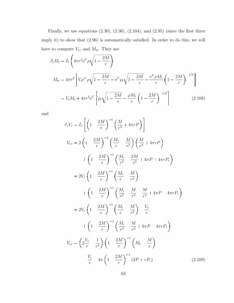
Finally, we use equations (2.30), (2.36), (2.104), and (2.95) (since the first three
imply it) to show that (2.96) is automatically satisfied. In order to do this, we will
have to compute Vrr and Mtt. They are
BtMt Bt
4πr2eV ρ
c1 2M
r
Mtt 4πr2
Vte
V ρ
c1 2M
r eV ρt
c1 2M
r eV ρMt
r
1 2M
r
12
VtMt 4πr2eV
ρt
c1 2M
r ρMt
r
1 2M
r
12(2.108)
and
BrVr Br
1 2M
r
1M
r2 4πrP
Vrr 2
1 2M
r
2Mr
r M
r2
M
r2 4πrP
1 2M
r
1Mr
r2 2M
r3 4πP 4πrPr
2Vr
1 2M
r
1Mr
r M
r2
1 2M
r
1Mr
r2 M
r3 M
r3 4πP 4πrPr
2Vr
1 2M
r
1Mr
r M
r2
Vr
r
1 2M
r
1Mr
r2 M
r3 8πP 4πrPr
Vrr
2Vrr 1
r2
1 2M
r
1Mr M
r
Vrr 4π
1 2M
r
1
p2P rPrq (2.109)
63

Making these substitutions into (2.96) yields
8πQ Vrr V 2
r Vrr
1 2M
r
M
rMr
1
r2 Vr
r
VtMt Mtt
re2V
1 2M
r
1
3M2t
r2e2V
1 2M
r
2
4πp2P rPrq V 2r
1 2M
r
Vr
r
Mr M
r
4πr
eV
ρt
1 2M
r
12 ρMt
r
1 2M
r
32
3M2t
r2e2V
1 2M
r
2
4πp2P rPrq Vr
M
r2 4πrP
Vr
r
Mr M
r
4πr
eV
ρt
1 2M
r
12 ρMt
r
1 2M
r
32
12πρMt
eV
1 2M
r
32
4πp2P rPrq 4πrVrP VrMr
r
4πrρteV
1 2M
r
12 8πρMt
eV
1 2M
r
32
4πp2P rPrq 4πrVrpP µq
4πrρteV
1 2M
r
12 8πρMt
eV
1 2M
r
32
64

4πp2P rPrq 4πrVrpP µq 8πρMt
eV
1 2M
r
32
4πr
Vrpµ P q Pr 2pP Qq
r
8πρMt
eV
1 2M
r
32
8πQ (2.110)
where the last two lines follow from using (2.104b). Thus so long as equation (2.104)
holds, equations (2.30), (2.36), and (2.95) imply equation (2.96). Since equations
(2.104), (2.30), and (2.36) imply equation (2.95) and equation (2.104) follows from
∇g T 0, we have that ∇g T 0 implies that solving equations (2.30) and (2.36) at
each time t is sufficient to solve the entire Einstein equation, which was the desired
result.
The proof of Lemma 2.3.1 follows.
Proof of Lemma 2.3.1. Recall equation (2.46). Then to compute the components of
T , we first have that
df ft dt fr dr peVc
1 2M
rdt fr dr (2.111)
df ft dt fr dr peVc
1 2M
rdt fr dr. (2.112)
Then, since g is diagonal, this implies that
|df |2 gpdf, dfq g
peV
c1 2M
rdt fr dr, pe
V
c1 2M
rdt fr dr
e2V
1 2M
r
pp gpdt, dtq frfr gpdr, drq
1 2M
r
|fr|2 |p|2 . (2.113)
65

With these facts, we now compute the quantities in question and do so in the same
order as they were presented. Thus we have the following.
T pνt, νtq µ0
2
Υ2dfpνtqdfpνtq
1 2M
r
|fr|2 |p|2Υ2
|f |2gpνt, νtq
µ0
2
Υ2
1 2M
r
pp |f |2
1 2M
r
|fr|2 |p|2Υ2
µ0
|f |2
1 2M
r
|fr|2 |p|2Υ2
. (2.114)
Next, because νη is an everywhere orthonormal basis,
T pνt, νrq µ0
1
Υ2
dfpνtqdfpνrq dfpνtqdfpνrq
1 2M
r
|fr|2 |p|2Υ2
|f |2gpνt, νrq
µ0
1
Υ2
1 2M
r
pfr frp
2µ0
Υ2
1 2M
r
Repfrpq. (2.115)
T pνr, νrq µ0
2
Υ2dfpνrqdfpνrq
1 2M
r
|fr|2 |p|2Υ2
|f |2gpνr, νrq
µ0
2
Υ2
1 2M
r
frfr
1 2M
r
|fr|2 |p|2Υ2
|f |2
µ0
|f |2
1 2M
r
|fr|2 |p|2Υ2
.
T pνθ, νθq µ0
2
Υ2dfpνθqdfpνθq
1 2M
r
|fr|2 |p|2Υ2
|f |2gpνθ, νθq
µ0
|f |2
1 2M
r
|fr|2 |p|2Υ2
. (2.116)
66

Finally,
T pνϕ, νϕq µ0
2
Υ2dfpνϕqdfpνϕq
1 2M
r
|fr|2 |p|2Υ2
|f |2gpνϕ, νϕq
µ0
|f |2
1 2M
r
|fr|2 |p|2Υ2
(2.117)
so that T pνϕ, νϕq T pνθ, νθq.
Finally, we prove Lemma 2.3.4.
Proof of Lemma 2.3.4. By equation (2.42) and Lemma 2.3.1, we have that
µ µ0
|f |2
1 2M
r
|fr|2 |p|2Υ2
(2.118a)
ρ 2µ0
Υ2
1 2M
r
Repfrpq (2.118b)
P µ0
|f |2
1 2M
r
|fr|2 |p|2Υ2
(2.118c)
Q µ0
|f |2
1 2M
r
|fr|2 |p|2Υ2
(2.118d)
We know from a previous proof that ∇g T 0 is equivalent to equation (2.104).
Moreover, by (2.47) and Lemma 2.3.3, we have that (2.45b) is equivalent to (2.53)
and (2.57). Thus it suffices to show that given (2.118), equations (2.53) and (2.57)
imply equation (2.104).
We will start with (2.104a). On one hand, the left hand side is equal to differen-
tiating (2.118a) with respect to t.
µt Btµ0
|f |2
1 2M
r
|fr|2 |p|2Υ2
µ0
ftf fft 2Mt
r
|fr|2 |p|2
Υ2
1 2M
r
frtfr frfrt ptp ppt
Υ2
67

µ0
eVc
1 2M
r
pf fp
2Mt
r
|fr|2 |p|2
Υ2
1 2M
r
frtfr frfrt ptp ppt
Υ2
µt µ0
p
feV
c1 2M
r pt
Υ2
1 2M
r
p
feV
c1 2M
r pt
Υ2
1 2M
r
2Mt
r
|fr|2 |p|2
Υ2
1 2M
r
frBrpeV
b1 2M
r
frBr
peV
b1 2M
r
Υ2
(2.119a)
On the other hand, we can substitute (2.118) into (2.104a).
µt 2ρeVc
1 2M
r
Vr 1
r
ρre
V
c1 2M
r Mt
r
1 2M
r
1
pµ P q
2eVc
1 2M
r
2µ0
Υ2
1 2M
r
Repfrpq
Vr 1
r
Br
2µ0
Υ2
1 2M
r
Repfrpq
eVc
1 2M
r 2Mtµ0
r
|fr|2 |p|2
Υ2
2µ0
Υ2eV
1 2M
r
32pfrp pfrq
Vr 1
r
µ0
Υ2Br
1 2M
r
pfrp pfrq
eVc
1 2M
r 2Mtµ0
r
|fr|2 |p|2
Υ2
pµ0
Υ2
1 2M
r
frVre
V
c1 2M
r 2fre
V
r
c1 2M
r
pµ0
Υ2
1 2M
r
frVre
V
c1 2M
r 2fre
V
r
c1 2M
r
68

µ0VreV
Υ2
1 2M
r
32 frp pfr
2Mtµ0
r
|fr|2 |p|2
Υ2
µ0eV
Υ2
c1 2M
r
pfrp pfrq Br
1 2M
r
1 2M
r
pfrrp pfrr frpr prfrq
pµ0
Υ2
1 2M
r
frVre
V
c1 2M
r frre
V
c1 2M
r 2fre
V
r
c1 2M
r
pµ0
Υ2
1 2M
r
frVre
V
c1 2M
r frre
V
c1 2M
r 2fre
V
r
c1 2M
r
µ0
Υ2
1 2M
r
Vre
V
c1 2M
r
frp pfr
2Mtµ0
r
|fr|2 |p|2
Υ2
µ0
Υ2
1 2M
r
eV pfrp pfrq
1 2M
r
12Br
1 2M
r
eVc
1 2M
rpfrpr prfrq
pµ0
Υ2
1 2M
r
frVre
V
c1 2M
r frre
V
c1 2M
r 2fre
V
r
c1 2M
r
pµ0
Υ2
1 2M
r
frVre
V
c1 2M
r frre
V
c1 2M
r 2fre
V
r
c1 2M
r
µ0
Υ2
1 2M
r
Vre
V
c1 2M
r
frp pfr
2Mtµ0
r
|fr|2 |p|2
Υ2
µ0
Υ2
1 2M
r
2eV pfrp pfrq Br
c1 2M
r
eVc
1 2M
rpfrpr prfrq
69

µt pµ0
Υ2
1 2M
r
Brfre
V
c1 2M
r
2fre
V
r
c1 2M
r
pµ0
Υ2
1 2M
r
Brfre
V
c1 2M
r
2fre
V
r
c1 2M
r
µ0
Υ2
1 2M
r
frBr
peV
c1 2M
r
frBr
peV
c1 2M
r
2Mtµ0
r
|fr|2 |p|2
Υ2
(2.119b)
Setting (2.119a) equal to (2.119b), we obtain
µ0
p
feV
c1 2M
r pt
Υ2
1 2M
r
p
feV
c1 2M
r pt
Υ2
1 2M
r
2Mt
r
|fr|2 |p|2
Υ2
1 2M
r
frBrpeV
b1 2M
r
frBr
peV
b1 2M
r
Υ2
pµ0
Υ2
1 2M
r
Brfre
V
c1 2M
r
2fre
V
r
c1 2M
r
pµ0
Υ2
1 2M
r
Brfre
V
c1 2M
r
2fre
V
r
c1 2M
r
µ0
Υ2
1 2M
r
frBr
peV
c1 2M
r
frBr
peV
c1 2M
r
2Mtµ0
r
|fr|2 |p|2
Υ2
70

p
Υ2feV
1 2M
r
12 pt
p
Υ2feV
1 2M
r
12 pt
p
Brfre
V
c1 2M
r
2fre
V
r
c1 2M
r
p
Brfre
V
c1 2M
r
2fre
V
r
c1 2M
r
0 p
pt Br
fre
V
c1 2M
r
eV
Υ2f
1 2M
r
12 2fr
r
c1 2M
r
p
pt Br
fre
V
c1 2M
r
eV
Υ2f
1 2M
r
12 2fr
r
c1 2M
r
(2.119c)
Note that, since V and M are real valued, the second term above is the complex
conjugate of the first term. Then by equation (2.53), equation (2.119c) holds.
Next, we consider (2.104b). We first differentiate (2.118b) with respect to t and
then compare it to (2.104b) after substituting (2.118), (2.49), and (2.50). This yields
ρt Bt
2µ0
Υ2
1 2M
r
Repfrpq
µ0
Υ2
4Mt
rRepfrpq
1 2M
r
frtp frtp frpt frpt
µ0
Υ2
# 4Mt
rRepfrpq
1 2M
r
p Br
peV
c1 2M
r
p BrpeV
c1 2M
r
frpt frpt
+
71

µ0
Υ2
# 4Mt
rRepfrpq
1 2M
r
p Br
peV
c1 2M
r
prpeV
c1 2M
r |p|2 Br
eVc
1 2M
r
frpt frpt
+
µ0
Υ2
# 4Mt
rRepfrpq
1 2M
r
Br|p|2 eV
c1 2M
r
|p|2 Br
eVc
1 2M
r
frpt frpt
+(2.120a)
From (2.104b), we obtain
ρt eVc
1 2M
r
Vrpµ P q Pr 2pP Qq
r
2ρMt
r
1 2M
r
1
4µ0Mt
rΥ2Repfrpq eV
c1 2M
r
2µ0Vr
Υ2
1 2M
r
p|fr|2 |p|2q
µ0Br |f |2
1 2M
r
|fr|2 |p|2Υ2
4µ0 |fr|2
rΥ2
1 2M
r
µ0eV
Υ2
1 2M
r
#2Vr |fr|2
c1 2M
r 2Vr |p|2
c1 2M
r
Υ2pfrf frfq
1 2M
r
12
1 2M
r
12Br
1 2M
r
|fr|2 |p|2
c
1 2M
rBr|fr|2 |p|2 4 |fr|2
r
c1 2M
r
+ 4µ0Mt
rΥ2Repfrpq
72

µ0
Υ2
1 2M
r
#fr
frVre
V
c1 2M
r
eV Υ2f
1 2M
r
12 2eV fr
r
c1 2M
r
fr
frVre
V
c1 2M
r eV Υ2f
1 2M
r
12 2eV fr
r
c1 2M
r
2VreV |p|2
c1 2M
r 2 |p|2 eV Br
c1 2M
r
eV
c1 2M
rBrp|p|2q
2 |fr|2 eV Brc
1 2M
r
eV
c1 2M
r
frrfr frfrr
+
4µ0Mt
rΥ2Repfrpq
µ0
Υ2
1 2M
r
#fr
Brfre
V
c1 2M
r
eV
Υ2f
1 2M
r
12 2fr
r
c1 2M
r
fr
Brfre
V
c1 2M
r
eV
Υ2f
1 2M
r
12 2fr
r
c1 2M
r
|p|2 Br
eVc
1 2M
r
Br
|p|2 eV
c1 2M
r
+ 4µ0Mt
rΥ2Repfrpq
(2.120b)
Equating (2.120a) and (2.120b) yields
µ0
Υ2
#4Mt
rRepfrpq
1 2M
r
Br|p|2 eV
c1 2M
r
|p|2Br
eVc
1 2M
r
frpt frpt
+
73

µ0
Υ2
1 2M
r
#fr
Brfre
V
c1 2M
r
eV
Υ2f
1 2M
r
12 2fr
r
c1 2M
r
fr
Brfre
V
c1 2M
r
eV
Υ2f
1 2M
r
12 2fr
r
c1 2M
r
|p|2 Br
eVc
1 2M
r
Br
|p|2 eV
c1 2M
r
+
4µ0Mt
rΥ2Repfrpq
0 fr
pt Br
fre
V
c1 2M
r
eV
Υ2f
1 2M
r
12 2fr
r
c1 2M
r
fr
pt Br
fre
V
c1 2M
r
eV
Υ2f
1 2M
r
12 2fr
r
c1 2M
r
(2.120c)
As before, since M and V are real valued, the second term above is the complex
conjugate of the first term. Then by equation (2.53), equation (2.120c) holds. Then
equations (2.53) and (2.57) imply equation (2.104) holds, which completes the proof.
74

3
Spherically Symmetric Static Statesof Wave Dark Matter
Now that we have described in detail spherically symmetric spacetimes and in partic-
ular presented some results about the spherically symmetric Einstein-Klein-Gordon
equations, we can now begin to comment on the subject of wave dark matter.
Describing the Einstein-Klein-Gordon equations in spherical symmetry is an ex-
cellent place to start studying wave dark matter for two reasons. First, it immensely
simplifies the equations involved making them easier to solve. Secondly, as mentioned
in the previous chapter, there are some very interesting objects to be described that
are approximately spherically symmetric. In the case of wave dark matter, dwarf
spheroidal galaxies are approximately spherically symmetric and almost entirely dark
matter (Walker et al. (2007); Mateo (1998)) implying that their kinematics are con-
trolled by their dark matter component. Thus determining what the wave dark
matter model predicts in spherical symmetry would be important in showing the
level of compatibility of wave dark matter with dwarf spheroidal galaxies.
The purpose of this chapter is to present a few results in this regard. In particular,
we describe an important class of spherically symmetric solutions of the Einstein-
75

Klein-Gordon equations called static states and discuss some properties of these
solutions. We should also reference here others’ results that, with the exception
of the ground state, these static states are unstable under perturbations (Seidel and
Suen (1990); Balakrishna et al. (1998); Bernal et al. (2010); Lai and Choptuik (2007);
Gleiser and Watkins (1989); Hawley and Choptuik (2000)), which poses a problem
in using the static states as a physical model. However, in physical situations dark
matter is always coupled with regular matter, which may have stabilizing effects
on the dark matter. Thus understanding the stability of these static states in the
presence of regular matter is an important open problem. It is also possible that dark
matter may not exist as a single static state at all and as such, finding other kinds of
stable configurations of wave dark matter is another important open problem. These
open problems are not addressed in this chapter, but are a goal of our future work
and one of the reasons for creating a program like the one presented in Chapter 5 to
evolve the spherically symmetric Einstein-Klein-Gordon equations in time.
3.1 The Spherically Symmetric Einstein-Klein-Gordon Equations
In this section, we discuss the Einstein-Klein-Gordon equations in spherical symme-
try on an asymptotically Schwarzschild spacetime.
To begin, let N be a spherically symmetric spacetime with metric g of the form in
equation (2.20). Additionally assume that N is asymptotically Schwarzschild, that is,
it is Schwarzschild as r Ñ 8. As in Chapter 2, define f : N Ñ C as a complex scalar
field on N such that pg, fq satisfies the Einstein-Klein-Gordon equations (2.45a) and
(2.45b). By Chapter 2, the spherically symmetric Einstein-Klein-Gordon equations
reduce to the system (2.58). Recall that by Proposition 2.3.6, equations (2.49) and
(2.51) are automatically satisfied by solving the system (2.58).
We note next the important behavior of the functions f, p, V, and M at the origin
and as r Ñ 8.
76

We use the previously mentioned fact that M is the flat integral of the energy
density to shed light on the initial behavior of the function M near the origin, r 0.
Using the construction in Chapter 2, the energy density of this system is defined as
µpt, rq T pνt, νtq, and the Einstein equation yields
Mpt, rq »Et,r
µpt, sq dV » r
0
4πs2µpt, sq ds. (3.1)
Since the energy density is spherically symmetric and smooth, if the energy density
is nonzero at the central value, r 0, at any time t, then the energy density must be
an even function of r. Moreover, since µpt, rq is also smooth at the origin, µrpt, 0q 0
for all t. Thus for small r, µ is approximately constant and nonnegative. Then the
above integral yields for small r that
Mpt, rq » r
0
4πs2µpt, sq ds » r
0
4πs2µpt, 0q ds 4πµpt, 0q3
r3 (3.2)
Thus the initial behavior of M near r 0 is that of a cubic power function. In
particular, this implies that for all t
Mpt, 0q 0, Mrpt, 0q 0, and Mrrpt, 0q 0 (3.3)
This is consistent with the fact that the metric functions, e2V and
1 2M
r
, are
also smooth spherically symmetric functions that are nonzero at r 0 and hence
even functions of r. This implies that, since r is an odd function, Mpt, rq must also
act like an odd function near r 0. Similarly, V pt, rq must be an even function of
r, implying that
Vrpt, 0q 0 (3.4)
for all t. Equation (3.3) implies via L’Hopital’s rule that
limrÑ0
M
r lim
rÑ0
M
r2 lim
rÑ0
Mr
r lim
rÑ0Mrr 0. (3.5)
77

Next, since f and p are spherically symmetric and allowed to be nonzero at r 0,
we have that both f and p are even functions in r as well, which, for regularity at
r 0, implies that
frpt, 0q 0 and prpt, 0q 0. (3.6)
for all t.
Next we consider the behavior of the functions at the outer boundary. Since N
is asymptotically Schwarzschild, there exist constants, m ¥ 0, called the total mass
of the system, and κ ¡ 0, and a Schwarzschild metric gS given by
gS κ2
1 2m
r
dt2
1 2m
r
1
dr2 r2 dσ2, (3.7)
such that g approaches gS as r Ñ 8. This yields the following asymptotic boundary
conditions.
2gSf Ñ Υ2f and f Ñ 0 as r Ñ 8 (3.8)
e2V Ñ κ2
1 2M
r
as r Ñ 8. (3.9)
The first boundary condition (3.8) implies by equation (2.58a) that Mr Ñ 0 as r Ñ 8and hence M approaches a constant value as r Ñ 8. Given equations (2.20), (3.7),
and the second boundary condition (3.9), this constant will be the parameter m in
(3.7).
Now that we have described the Einstein-Klein-Gordon equations and its asymp-
totically Schwarzschild boundary conditions in spherical symmetry, we are ready to
discuss the class of spherically symmetric solutions to the Einstein-Klein-Gordon
equations that yield static metrics.
78

3.2 Spherically Symmetric Static States
In the remainder of this chapter, we will consider solutions of the spherically sym-
metric Einstein-Klein-Gordon equations where the scalar field f is of the form
fpt, rq eiωtF prq (3.10)
where ω P R and F is complex-valued. As t increases, f rotates the values of the
function F prq through the complex plane with angular frequency ω without changing
their absolute value. Thus, without loss of generality, we will assume that ω ¥ 0,
since if ω 0, F will simply rotate in the opposite direction. With f of this form,
we have that
fr eiωtF 1prq (3.11)
p eV
1 2M
r
12ft
eV
1 2M
r
12 iωeiωtF prq . (3.12)
With a scalar field of this form, the system (2.58) implies that the metric is static
under certain conditions on the function F . We collect this result in the following
proposition.
Proposition 3.2.1. Let pN, gq be a spherically symmetric asymptotically Schwarz-
schild spacetime that satisfies the Einstein-Klein-Gordon equations (2.45) for a scalar
field of the form in (3.10). Additionally, assume that F prq hprqeiaprq for smooth
real-valued functions h and a, where h has only isolated zeros, if any. Then pN, gqis static if and only if aprq is constant.
Proof. By definition, a spacetime metric is static if there exists a timelike Killing
vector field and a spacelike hypersurface that is orthogonal to the Killing vector
79

field. For the metric in equation (2.20), if the metric components, V and M , do
not depend on t, then Bt is one such Killing vector field and it is already orthogonal
to the t constant spacelike hypersurfaces. If a spherically symmetric metric is
static, then we can choose the t coordinate to be in the direction of the timelike
Killing vector field, making Bt the timelike Killing vector field in these coordinates,
and choose the polar-areal coordinates on its orthogonal spacelike hypersurfaces,
yielding a metric of the form in (2.20). Then since the metric cannot change in the
direction of Bt, the metric components must be t-independent. It remains then to
show that under and only under the given conditions on F , the metric components
are t-independent.
Note that by equation (2.49), Mt 0 if and only if Repfrpq 0. Using equation
(3.11) and (3.12), we obtain
Repfrpq Re
eiωtF 1prqeV
1 2M
r
12 iωeiωtF prq
eV
1 2M
r
12RepiωF 1prqF prqq (3.13)
Thus Repfrpq 0 if and only if RepiωF 1prqF prqq 0, which is true if and only if
F 1prqF prq is real-valued. By assumption, F prq can be written as
F prq hprqeiaprq (3.14)
for smooth real-valued functions h and a. If we write F prq this way, then F 1prq is as
follows.
F 1prq h1prqeiaprq ihprqa1prqeiaprq eiaprq ph1prq ihprqa1prqq . (3.15)
Then we have that
F 1prqF prq h1prqhprq ihprq2a1prq. (3.16)
80

Since h and a are both real-valued, we see that F 1prqF prq is real if and only if
hprq2a1prq 0. Since h has only isolated zeros, hprq2a1prq 0 if and only if a1prq 0
or equivalently aprq is constant.
It suffices from here to show that Mt 0 if and only if g is t-independent.
Obviously, g being t-independent implies Mt 0. On the other hand, assume that
Mt 0. First note that, since Mt 0, Mrt 0 as well. Moreover, since |f |2 |F |2
and |fr|2 |F 1|2 and F has zero t-derivative, then |f |2 and |fr|2 both have zero
t-derivatives. Differentiating (2.58a) with respect to t and using the fact that |f |2,
|fr|2, and M all have zero t-derivatives, we have that
Mrt 4πr2µ0
Bt|f |2 2Mt
r
|fr|2 |p|2Υ2
1 2M
r
Bt|fr|2 Bt
|p|2Υ2
0 4πr2µ0
1 2M
r
Bt|p|2Υ2
. (3.17)
Thus since, M , Υ, and µ0 are all nonzero, Bt|p|2 0.
Next, since (2.58a) and (2.58b) completely determine the Einstein equation, the
function V is determined at every value of t by solving (2.58b) at that value of t.
Since |f |2, |fr|2, |p|2, and M never change with t, Vr never changes with t and hence
the solution, V , of (2.58b), by uniqueness of the solution to an ODE, will never
change with t so long as V pt, 0q constant. Since V pt, 0q is determined to be the
value that makes V satisfy (3.9) and since M never changes with t, then the fact
that Vr is t-independent forces V pt, 0q constant. Thus Vt 0 and the metric is
t-independent.
Since the value of a simply adjusts the “starting position” of the values of f
before they rotate, we will, without loss of generality, set a 0, which is the same
assumption that F prq be real-valued. This amounts to simply choosing the hyper-
surface that we denote as t 0. To summarize, we restrict our attention to static
81

states of the form in (3.10) with ω ¥ 0 and F real-valued.
3.2.1 ODEs for Static States
In this section, we input our ansatz (3.10) with the requirement that ω ¥ 0 and F
is real-valued into the Einstein-Klein-Gordon equations (2.58a)-(2.58d). Since the
metric is t-independent, we summarize that
V V prq, M Mprq, fpt, rq eiωtF prq. (3.18)
Also note that by (3.10)-(3.12),
|f | |F | , (3.19)
|fr| |F 1| , (3.20)
|p| eV
1 2M
r
12 iωeiωtF
|F |ωeV
1 2M
r
12. (3.21)
Additionally, if we differentiate (3.12) with respect to t and (3.11) with respect to r,
we obtain,
pt Bt
eV
1 2M
r
12 iωeiωtF
ω2eV
1 2M
r
12eiωtF (3.22)
frr eiωtF 2 (3.23)
Then equations (2.58a) and (2.58b) become
M 1 4πr2µ0
1 ω2
Υ2e2V
|F |2
1 2M
r
|F 1|2Υ2
(3.24)
V 1
1 2M
r
1#M
r2 4πrµ0
1 ω2
Υ2e2V
|F |2
1 2M
r
|F 1|2Υ2
+
(3.25)
82

Equation (2.58c) turns into (3.12), thereby becoming redundant. The last equation,
(2.58d), becomes
ω2eV
1 2M
r
12eiωtF eV
Υ2
1 2M
r
12eiωtF
2eiωtF 1
r
c1 2M
r
V 1eV eiωtF 1c
1 2M
r eV eiωtF 2
c1 2M
r
eV eiωtF 1
1
2
1 2M
r
122M
r2 2M 1
r
ω2eV
1 2M
r
12eiωtF eV
#1 2M
r
12 2eiωtF 1
M
r2 4πrµ0 |F |2
Υ2eiωtF
c
1 2M
r
eiωtF 2 2
reiωtF 1
+
ω2F e2V
2F 1
M
r2 4πrµ0 |F |2
Υ2F
1 2M
r
F 2 2
rF 1
e2V
1 2M
r
F 2 e2V
Υ2 ω2
e2V
F
2F 1
1
r M
r2 4πrµ0 |F |2
(3.26)
which yields
F 2
1 2M
r
1 Υ2 ω2
e2V
F 2F 1
M
r2 4πrµ0 |F |2 1
r
(3.27)
83

To make the system first order, we will introduce a new function Hprq F 1prq. Then
(3.24), (3.25), and (3.27) become the system
M 1 4πr2µ0
1 ω2
Υ2e2V
|F |2
1 2M
r
|H|2Υ2
(3.28a)
V 1
1 2M
r
1#M
r2 4πrµ0
1 ω2
Υ2e2V
|F |2
1 2M
r
|H|2Υ2
+
(3.28b)
F 1 H (3.28c)
H 1
1 2M
r
1 Υ2 ω2
e2V
F 2H
M
r2 4πrµ0 |F |2 1
r
(3.28d)
3.2.2 Boundary Conditions
We will solve the system (3.28) numerically, but in order to do so, we need to ex-
press how we will deal with our boundary conditions numerically. Ideally, we would
like to model the system in an infinite spacetime, but since we are computing these
solutions numerically, we must introduce an artificial right hand boundary, say at
r rmax, to which we restrict our domain. To simulate the fact that the space-
time is asymptotically Schwarzschild, which we detailed in (3.8) and (3.9), we will
choose rmax sufficiently large and impose the condition that the spacetime be ap-
proximately Schwarzschild at the boundary. That is, we will impose (3.8) and (3.9)
at the boundary r rmax.
In this case, equation (3.9) at r rmax becomes
e2V prmaxq κ2
1 2Mprmaxq
rmax
0 V prmaxq 1
2ln
1 2Mprmaxq
rmax
lnκ (3.29)
For (3.8) at r rmax, we require f to approximately solve the Klein-Gordon
equation (2.45b) in the Schwarzschild metric (3.7). Computing the Laplacian in the
84

Schwarzschild metric, this equation becomes
1 2m
r
2
F 2
1 2m
r
1 2m
r
2F 1
r
Υ2
1 2m
r
ω2
κ2
F 0.
(3.30)
For large r, this simplifies to
F 2 2F 1
r
Υ2 ω2
κ2
F 0. (3.31)
This ODE is routinely solved and has the general solution
F C1
rerb
Υ2ω2
κ2 C2
rerb
Υ2ω2
κ2 (3.32)
for some constants C1, C2 P R.
We will show that this is consistent with the Wentzel-Kramers-Brillouin (WKB)
approximation (Wentzel (1926); Kramers (1926); Billouin (1926)) of the solution to
equation (3.30) as r Ñ 8, if we also assume that m ! 1 (in mass units of years).
Following the procedure outlined in the book by Bender and Orszag (Bender
and Orszag (1978)), we have the following. See also Carlini (1817); Liouville (1837);
Green (1838) for more references on this method.
Since
1 2m
r
¡ 0 for all r, we can rewrite equation (3.30) as
F 2
1
r 1
r
1 2m
r
1F 1
Υ2
1 2m
r
1
ω2
κ2
1 2m
r
2F 0
(3.33)
Define two new functions ξ and ζ as follows.
ξprq 1
r 1
r
1 2m
r
1
(3.34)
ζprq Υ2
1 2m
r
1
ω2
κ2
1 2m
r
2
(3.35)
85

which allows us to rewrite (3.33) as
F 2 ξF 1 ζF 0 (3.36)
To compute the leading term of the solution to (3.36) as r Ñ 8, make the substitu-
tion
F prq eSprq, where Sprq S0prq S1prq S2prq (3.37)
with
S0prq " S1prq " S2prq " (3.38)
as r Ñ 8. To compute the WKB approximation, we will compute the values of S0
and S1 in this expansion. As is standard, we will also make the assumption that
S2 ! pS 1q2. (3.39)
Making this substitution in (3.36) yields as r Ñ 8F 2 ξF 1 ζF
eSS2 pS 1q2 ξeSS 1 ζeS
S2 pS 1q2 ξS 1 ζ
pS 1q2 ξS 1 ζ
S 1 ξ2 1
2
aξ2 4ζ. (3.40)
For this next step, we will compute the asymptotic expansion of the right hand side.
The asymptotic expansion of some function Bprq is defined as
Taylors0
Bpsq
s 1
r
(3.41)
where Bpsq Bp1sq and Taylors0 denotes the Taylor expansion centered at s 0.
If we let
Q c
Υ2 ω2
κ2
1 ω2
Υ2κ2 ω2
(3.42)
86

Then the asymptotic expansion of the right hand side of (3.40), whose computation
we have suppressed, is
ξ
2 1
2
aξ2 4ζ
cΥ2 ω2
κ2 1
r mQ
rO
1
r2
. (3.43)
Thus as r Ñ 8,
S 1 c
Υ2 ω2
κ2 1
r mQ
rO
1
r2
(3.44)
which is consistent with our approximation that S2 ! pS 1q2. Equation (3.44) yields
S rc
Υ2 ω2
κ2 ln r mQ ln r lnC O
1
r
(3.45)
for some real constant C ¡ 0. Thus we have
S0 rc
Υ2 ω2
κ2 lnC (3.46)
S1 ln r mQ ln r (3.47)
This yields that the leading term of F is of the form
CrmQ
rerb
Υ2ω2
κ2 . (3.48)
Thus as r Ñ 8, the WKB approximation of the solution to (3.30) will be of the form
F C1rmQ
rerb
Υ2ω2
κ2 C2rmQ
rerb
Υ2ω2
κ2 . (3.49)
However, in practice, the solutions we will be considering will usually have total
mass values m ! 1 (for a few examples of total mass values of solutions see Figure
4.5). Under these circumstances, the above WKB approximation can be further
approximated by
F C1
rerb
Υ2ω2
κ2 C2
rerb
Υ2ω2
κ2 (3.50)
87

which is exactly what we have in (3.32). It is important to note here, however,
that if the mass value m is not sufficiently small, requiring equation (3.50) would
no longer maintain that the scalar field asymptotically satisfied the Klein-Gordon
equation in the Schwarzschild metric. We would instead need to impose the entire
WKB approximation in (3.49) to get the appropriate asymptotics. For our work
here, though, we will use equation (3.50), or equivalently, equation (3.32).
Now we also require that F Ñ 0 as r Ñ 8 so that f Ñ 0 as well. Thus C1 0
and we relabel C2 as simply C. That is, at r rmax, we require
F C
rerb
Υ2ω2
κ2 . (3.51)
We have no way of directly determining the correct value of C in equation (3.51)
associated with a given static solution. However, if we differentiate equation (3.51)
with respect to r, we obtain
F 1 Cr
erb
Υ2ω2
κ2
cΥ2 ω2
κ2 C
r2erb
Υ2ω2
κ2
c
Υ2 ω2
κ2 1
r
F (3.52)
which does not depend on C. Then the condition that at r rmax, f approximately
satisfies the Klein-Gordon equation with the Schwarzschild background metric re-
duces to requiring that
F 1prmaxq c
Υ2 ω2
κ2 1
rmax
F prmaxq 0. (3.53)
This condition imposes that F is decaying appropriately to 0. It also puts a restriction
on the possible values of ω. Since the left hand side of the above equation must be
real, we have that Υ2 ω2
κ2¥ 0, or equivalently,
ωκ
ω
κ¤ Υ (3.54)
88

That is, ωκ P r0,Υs. In our numerical calculations, we normalize this quantity and
keep track ofω
κΥP r0, 1s instead.
Next we consider the boundary at the origin r 0. We have already noted above
that Mp0q 0. Moreover, since frpt, 0q 0 for all t,
Hp0q F 1p0q eiωtfrpt, 0q 0. (3.55)
Note that by the system (3.28), Hp0q 0 implies that if F p0q 0, then F prq 0
for all r, since H 1prq and F 1prq will never change. We are interested in non-trivial
solutions to these equations so we require that F p0q 0. However, for any constants
c and µ, if cf is a solution to the Einstein-Klein-Gordon equations, (2.45), with
µ0 µ, then f is a solution to the Einstein-Klein-Gordon equations with µ0 c2µ.
Thus, without loss of generality, we will set F p0q 1 absorbing any excess factors
into µ0.
At this point, we have four remaining parameters to choose, namely, V p0q, ω,
Υ, and µ0. By requiring (3.29) and (3.53), two of these values are determined,
leaving two remaining degrees of freedom. The parameter Υ is an as yet unknown
fundamental constant, making it important in our computations to be able to freely
set Υ so that we can test different values and see how they match the data. The
parameter µ0 controls the magnitude of the energy density and so seems a natural
choice as another parameter to freely choose. However, this choice is not the only
choice that could be made. For example, one could instead freely choose Υ and ω
and use the boundary conditions to pin down V p0q and µ0 with equivalent results.
When freely choosing Υ and µ0, to compute the other two parameters, V p0qand ω, we solve a shooting problem to satisfy the desired boundary conditions. We
illustrate next in detail how we performed this shooting procedure. However, first,
we summarize the information about the boundary conditions.
89

For some choice of Υ and µ0, we require at r 0,
F p0q 1, Hp0q 0, Mp0q 0, V p0q V0, (3.56)
and choose ω and V0 to satisfy
F 1prmaxq c
Υ2 ω2
κ2 1
rmax
F prmaxq 0, (3.57)
V prmaxq 1
2ln
1 2Mprmaxq
rmax
lnκ 0. (3.58)
For simplicity in our calculations, we set κ 1. Then we use the standard forward
Euler method to solve the system (3.28) with these boundary conditions.
To understand the procedure we used to solve the shooting problems mentioned
above, we first comment about what equation (3.27) tells us about the behavior of
F in our system. We are solving these equations in the low field limit where the
metric (2.20) is close to Minkowski. That is, both V and M are approximately zero.
Recall that equation (3.27) came immediately from equation (3.26), which results
from substituting (3.10) into (2.58d). Letting V M 0 makes equation (2.58d)
and the first line of equation (3.26) reduce to
∆rF Υ2 ω2
F (3.59)
where ∆r is the Laplacian in R3 in spherical coordinates. The one dimensional
analogue to the above equation is
Fxx kF. (3.60)
The solution of this differential equation depends on the sign of k. If k ¡ 0, then
the solutions either exponentially grow or decay. If k 0, the solutions exhibit
oscillatory behavior. In equation (3.27), the analogous coefficient that will control
whether the solutions exhibit oscillatory or exponential behavior is the following,
90

which we will denote as λprq.
λprq
Υ2 ω2
e2V prq
. (3.61)
The sign of λprq depends on r. While λprq 0, the solution of (3.27) will exhibit
oscillatory behavior. On the other hand, while λprq ¡ 0, the solution of (3.27) will
exhibit exponential growth or decay.
Since Υ and ω are constants, the sign of λprq is completely controlled by the
expp2V q term. If V is strictly increasing and starts low enough, then for small r,
expp2V q will be small yielding that λprq 0 and the initial part of the solution
will oscillate. Then as r increases, expp2V q will eventually be large enough that the
Υ2 term dominates λprq making λprq ¡ 0 and the end behavior will be exponen-
tial growth or decay. Imposing boundary condition (3.57) will ensure decaying end
behavior instead of growth.
The two parameters that control where this change from oscillation to exponential
decay occurs are the initial value of V and the parameter ω. Larger values of ω and
lower values of V p0q will increase the length of the oscillating region and push the
point where it changes to exponential decay out to larger radii. In fact, given a
fixed Υ and µ0, for each value of V p0q, there is a discrete infinite set of ω values for
which each ω in the set corresponds to a solution F that has a given number of zeros
(caused by a lengthening of the oscillating region) and the appropriate end behavior.
Thus we perform our shooting problem as follows. To find a solution with say
n zeros, first, fix a choice of Υ and µ0. Then pick a value of V p0q V0. Since
we have set κ 1, ω Υ in order to be able to satisfy equation (3.57). Then we
systematically pick different values of ω in the interval r0,Υs until we obtain the
appropriate number of zeros and satisfy (3.57). Finally, we use a Newton’s method
approach to find the value of V0 whose corresponding solution with n zeros yields a
91

potential function satisfying (3.58).
These solutions, now characterized by the number of zeros the resulting scalar
field has, are referred to as spherically symmetric state states of wave dark matter.
A static state with no zeros is called a ground state; with one zero, it is called a
first excited state; with two, it is called a second excited state, and so forth. There
is a considerable amount known about static states as they have been studied for
decades, see Bernal et al. (2010); Seidel and Suen (1990); Balakrishna et al. (1998);
Gleiser and Watkins (1989); Hawley and Choptuik (2000); Lai and Choptuik (2007)
for just a few examples. In the remaining sections, we will present some useful results
about these static states.
3.2.3 Plots of Static States
In Figures 3.1 to 3.4, we have plotted examples of the scalar field F prq (see Figure
3.1), Mass Mprq (see Figure 3.2), energy density µprq (see Figure 3.3), and gravi-
tational potential V prq (see Figure 3.4) for a generic ground state and first through
third excited states. We make here the following three observations. First, in these
plots, V is strictly increasing, as expected, and M approaches a constant value as
r Ñ 8, also as we expected. Second, for each zero of the function F , there is a zero
of the energy density plot µ, a ripple in the mass profile M , and slight but rapid
change in the slope of the potential V . And finally, the energy density appears to be
approximately proportional to |F |2 |f |2.
3.3 Families of Static States
We explained above that four parameters control what static solution is generated by
the equations. However, since we require two conditions on the boundary, choosing
only two of these parameters will define a static state. As stated before, we choose
to define Υ and µ0 and solve the shooting problem for the parameters V0 and ω. For
92

Figure 3.1: Plots of static state scalar fields (specifically the function F prq in(3.10)) in the ground state and first, second, and third excited states. Note thenumber of nodes (zeros) of each function.
each n, this defines a function, Sn : R2 Ñ R2, which maps the pair pΥ, µ0q to the
pair pV0, ωq such that the choices Υ, µ0, V0, ω yields an nth excited state (n 0, of
course, referring to the ground state).
A natural question to ask here would be “Is there an expression for Sn for each
n?” The answer to this question is yes, at least in the low field limit. In fact, we
have also found expressions for the total mass m of the system and the half-mass
radius rh, that is, the radius rh for which Mprhq m2. These expressions were
found by numerically computing the states for several different values of Υ and µ0,
all of which yield a state in the low field limit. We analyzed the resulting values and
93
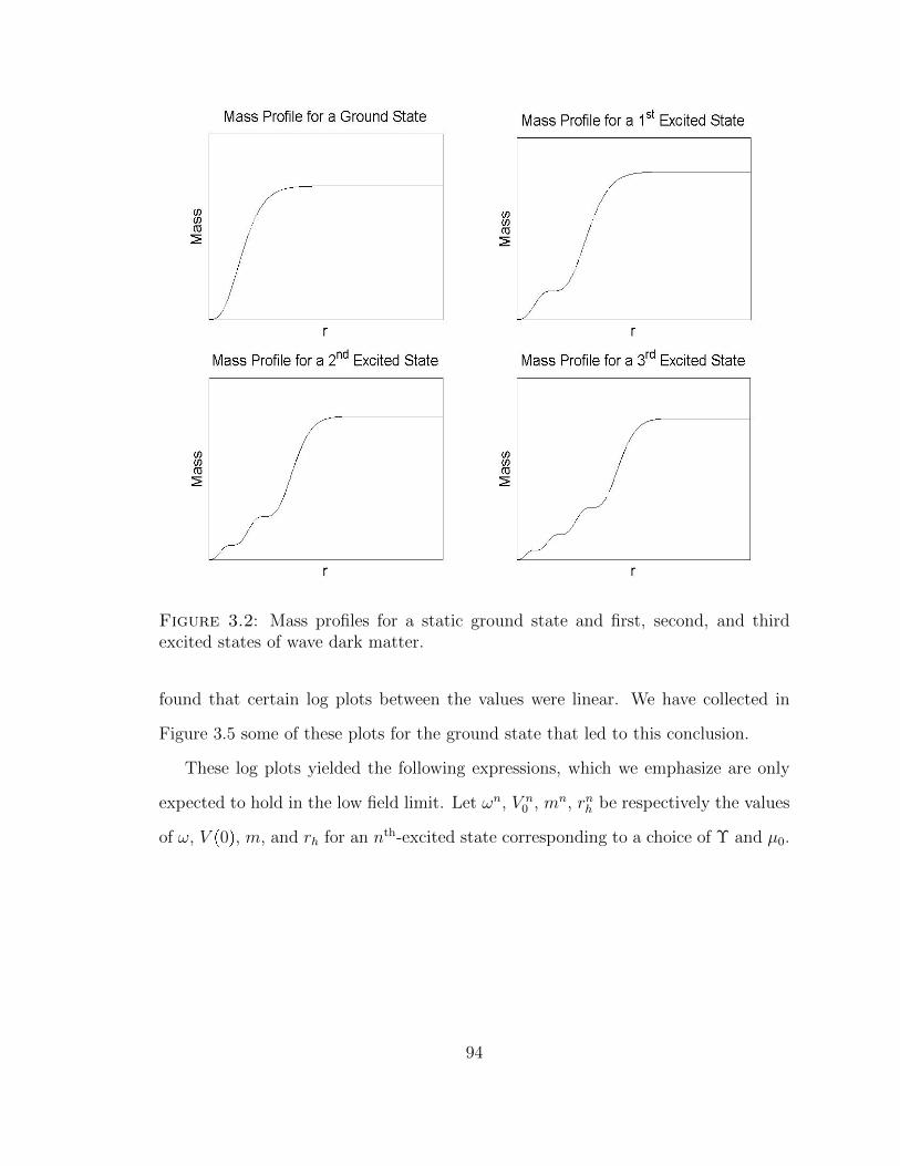
Figure 3.2: Mass profiles for a static ground state and first, second, and thirdexcited states of wave dark matter.
found that certain log plots between the values were linear. We have collected in
Figure 3.5 some of these plots for the ground state that led to this conclusion.
These log plots yielded the following expressions, which we emphasize are only
expected to hold in the low field limit. Let ωn, V n0 , mn, rnh be respectively the values
of ω, V p0q, m, and rh for an nth-excited state corresponding to a choice of Υ and µ0.
94

Figure 3.3: Energy density profiles for a static ground state and first, second, andthird excited states of wave dark matter.
Then we have that
ωnpΥ, µ0q Υ exp
Cnfrequency
?µ0
Υ
(3.62a)
V n0 pΥ, µ0q Cn
potential
?µ0
Υ(3.62b)
mnpΥ, µ0q CnmassΥ
32µ140 (3.62c)
rnhpΥ, µ0q CnradiusΥ
12µ140 (3.62d)
for some constants Cnfrequency, C
npotential, C
nmass and Cn
radius which depend only on n.
We have computed these constants for the ground through fifth excited states as
well as for the tenth and twentieth excited states and have collected their values in
95

Figure 3.4: Plots of the potential function, V , for a static ground state and first,second, and third excited states of wave dark matter.
Table 3.1. Note also that equations (3.62a) and (3.62b) constitute the Sn function
mentioned above.
In the wave dark matter model, Υ is a fundamental constant that should be the
same throughout the universe. In the case of constant Υ, for each n, the equations
in (3.62) define one-parameter families of the nth excited states, the parameter being
the scaling constant µ0. For constant Υ then, we have that these static states only
differ in size where, by equations (3.62c) and (3.62d), a larger µ0 corresponds to a
more massive and more dense wave dark matter halo.
96
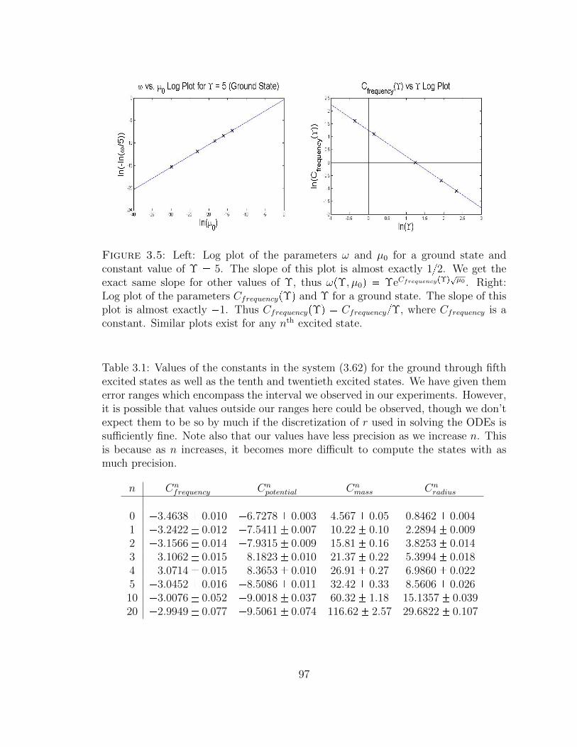
Figure 3.5: Left: Log plot of the parameters ω and µ0 for a ground state andconstant value of Υ 5. The slope of this plot is almost exactly 12. We get theexact same slope for other values of Υ, thus ωpΥ, µ0q ΥeCfrequencypΥq
?µ0 . Right:
Log plot of the parameters CfrequencypΥq and Υ for a ground state. The slope of thisplot is almost exactly 1. Thus CfrequencypΥq CfrequencyΥ, where Cfrequency is aconstant. Similar plots exist for any nth excited state.
Table 3.1: Values of the constants in the system (3.62) for the ground through fifthexcited states as well as the tenth and twentieth excited states. We have given themerror ranges which encompass the interval we observed in our experiments. However,it is possible that values outside our ranges here could be observed, though we don’texpect them to be so by much if the discretization of r used in solving the ODEs issufficiently fine. Note also that our values have less precision as we increase n. Thisis because as n increases, it becomes more difficult to compute the states with asmuch precision.
n Cnfrequency Cn
potential Cnmass Cn
radius
0 3.4638 0.010 6.7278 0.003 4.567 0.05 0.8462 0.0041 3.2422 0.012 7.5411 0.007 10.22 0.10 2.2894 0.0092 3.1566 0.014 7.9315 0.009 15.81 0.16 3.8253 0.0143 3.1062 0.015 8.1823 0.010 21.37 0.22 5.3994 0.0184 3.0714 0.015 8.3653 0.010 26.91 0.27 6.9860 0.0225 3.0452 0.016 8.5086 0.011 32.42 0.33 8.5606 0.02610 3.0076 0.052 9.0018 0.037 60.32 1.18 15.1357 0.03920 2.9949 0.077 9.5061 0.074 116.62 2.57 29.6822 0.107
97
3.3.1 Scalings of Static States
Certain scalings exist for various quantities if we scale time and length in any coor-
dinate system. In particular, let us scale the time coordinate, t, and the standard
spatial coordinates, xi, so that
Time: t βt Distance: xi αxi (3.63)
for some positive constants β, α P R. Then velocities in the pt, xq system will scale
to velocities in the pt, xq system as follows
vi dxi
dt α
β
dxi
dt α
βvi (3.64)
Similarly, other quantities scale as follows (velocity is included again for complete-
ness).
Velocity: v α
βv Mass: m α3
β2m
Energy Density: µ 1
β2µ Gravitational Potential: V α2
β2V
Frequency: λ 1
βλ (3.65)
These scalings are routine to derive and follow directly from how the units on each of
these quantities scale with the scaling for mass being that which is required to keep
the universal gravitational constant the same from one scaled coordinate system to
the other.
From the system (3.62), the scalings in (3.63) and (3.65), and given that the
constants Cn are dimensionless, we infer how the parameters µ0 and Υ would scale
under these coordinate scalings in order to keep (3.62) invariant. To do this, let c1
and c2 be such that under the coordinate scalings in (3.63),
µ0 c1µ0 and Υ c2Υ. (3.66)
98

Since m and rh are a mass and spatial quantity respectively, equations (3.62c) and
(3.62d) yield
mn α3
β2mn
α3
β2CnmassΥ
32µ140
α3
β2Cnmassc
322 Υ32c14
1 µ140
α3c322
β2c141
CnmassΥ
32µ140 (3.67)
and
rnh αrnh
αCnradiusΥ
12µ140
αCnradiusc
122 Υ12c14
1 µ140
αc122 c
141 Cn
radiusΥ12µ14
0 (3.68)
Then requiring these equations to be invariant under coordinate scalings is equivalent
to
α3c322
β2c141
1 and αc122 c
141 1 (3.69)
Solving these two equations simultaneously for c1 and c2 yields
c1 1
β2and c2 β
α2. (3.70)
Thus equations (3.62c) and (3.62d) imply that µ0 and Υ scale as follows
Stress Energy Tensor Constant: µ0 1
β2µ0 Upsilon: Υ β
α2Υ. (3.71)
99

We observe here that µ0 scales as energy density, which is expected given that as we
said before it controls the magnitude of the energy density function defined by the
stress energy tensor.
Since Υ is a fundamental constant in this system, it is appropriate to ask under
what kinds of coordinate scalings of the form in (3.63) is Υ invariant, that is, Υ Υ.
In light of (3.71), the answer to this question is readily apparent, those scalings where
β α2. Under this type of scaling, (3.63), (3.65), and (3.71) become
Time: t α2t Distance: x αx
Velocity: v 1
αv Mass: m 1
αm
Energy Density: µ 1
α4µ Gravitational Potential: V 1
α2V
Frequency: λ 1
α2λ
Stress Energy Tensor Constant: µ0 1
α4µ0 Upsilon: Υ Υ.
(3.72)
The scalings in (3.72) are also consistent with keeping the remaining relations
(3.62a) and (3.62b) invariant under coordinate scalings. Showing this for (3.62b)
is straightforward and follows from (3.72) and the fact that V0 has gravitational
potential units,
V n0 Cn
potential
?µ0
Υ
α2
β2V n
0 Cnpotential
aβ2µ0
βα2Υ
α2
β2V n
0 Cnpotential
α2
β2
?µ0
Υ
V n0 Cn
potential
?µ0
Υ. (3.73)
100

We should note that the above holds even if we do not assume that β α2. However,
the invariance of the next equation does rely on the fact that β α2. In fact, it
relies on the form the static Einstein-Klein-Gordon equations take in the low field
limit.
Specifically, consider a static spacetime in the low field Newtonian limit and
assume its static metric can be written in the form
g V pxq2 dt2 V pxq2 dx2 (3.74)
where dx2 is the flat metric on R3 and V 1. Additionally, assume the spacetime
is in the presence of a scalar field fpt,xq which can be written of the form
fpt,xq eiΥtF pt,xq (3.75)
where F has small time derivative and changes little on the scale of 1Υ
. Under these
assumptions, the Einstein-Klein-Gordon equations reduce to the following system of
equations
∆R3V 4π
2µ0
F 2 (3.76)
iBFBt 1
2Υ∆R3F ΥV F (3.77)
where V V 1. This system is called the Poisson-Schrodinger equations. In
spherical symmetry, we would write this scalar field as fpt, rq eiΥtF pt, rq and since
the metric is static, the spherically symmetric static state would be contained in this
class of solutions. Since the static states are of the form fpt, rq eiωtF prq, we have
that
F pt, rq eipωΥqtF prq. (3.78)
Thus the angular frequency of the scalar field F in the Poisson-Schrodinger equations
is ω Υ. Being a frequency in the low field limit, we would expect this to scale
according to (3.72).
101

We now have what we need to show that (3.62a) is invariant under the scalings
in (3.72). Since (3.62a) is not a power function, we approximate the equation to first
order using the Taylor expansion of ex and show that the approximate equation is
invariant which implies that the original equation is approximately invariant. This
is sufficient since all of the equations in (3.62) are only approximations anyway.
ωn Υ exp
Cnfrequency
?µ0
Υ
ωn Υ Υ exp
Cnfrequency
?µ0
Υ
Υ
1
α2pωn Υq Υ ΥCn
frequency
?µ0
Υ Υ
Cnfrequency
?µ0
Cnfrequency
cµ0
α4
1
α2pωn Υq 1
α2Cnfrequency
?µ0
ωn Υ Cnfrequency
?µ0
ωn ΥΥCnfrequency
?µ0
Υ
ωn Υ exp
Cnfrequency
?µ0
Υ
. (3.79)
3.3.2 Properties of Static State Mass Profiles
In this last section, we discuss a few additional properties of static state mass profiles
that are of particular interest to the study of wave dark matter. The first is the
relationship between the total mass m and the half-mass radius rh for any nth excited
state. We observe from equations (3.62c) and (3.62d) that the product mrh does not
102

Figure 3.6: Left: Plot of the mass profile of a ground state with its correspondinghyperbola of constant Υ overlayed. Any ground state mass profile that keeps thepresented relationship with this hyperbola corresponds to the same value of Υ. Right:Examples of different ground state mass profiles corresponding to the same value ofΥ. The corresponding hyperbola of constant Υ is overlayed. Notice that all threemass profiles have the same relationship with the hyperbola.
depend on the parameter µ0. Specifically,
mrh CmassCradiusΥ2
, (3.80)
where we have suppressed the notation of n. If Υ is constant, then, because both
Cmass and Cradius are positive for all n (see Table 3.1), the right hand side of this
equation is some positive constant, k, and we have that
mrh k, (3.81)
which defines a hyperbola. Thus, for a given nth excited state, all of the possible
mass profiles for a constant value of Υ lie along a hyperbola. We illustrate this
phenomenon in Figure 3.6.
Another property of interest is the initial behavior of a static state mass profile.
We explained previously that the mass function of any spherically symmetric solution
to the Einstein-Klein-Gordon equations is initially cubic and approximately equal to
the value in equation (3.2). It is routine to show that, for a static state, the value
of µpt, 0q µp0q (since the metric and stress energy tensor for a static state is
103
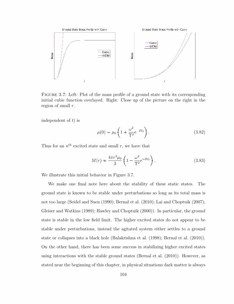
Figure 3.7: Left: Plot of the mass profile of a ground state with its correspondinginitial cubic function overlayed. Right: Close up of the picture on the right in theregion of small r.
independent of t) is
µp0q µ0
1 ω2
Υ2e2V0
. (3.82)
Thus for an nth excited state and small r, we have that
Mprq 4πr3µ0
3
1 ω2
Υ2e2V0
. (3.83)
We illustrate this initial behavior in Figure 3.7.
We make one final note here about the stability of these static states. The
ground state is known to be stable under perturbations so long as its total mass is
not too large (Seidel and Suen (1990); Bernal et al. (2010); Lai and Choptuik (2007);
Gleiser and Watkins (1989); Hawley and Choptuik (2000)). In particular, the ground
state is stable in the low field limit. The higher excited states do not appear to be
stable under perturbations, instead the agitated system either settles to a ground
state or collapses into a black hole (Balakrishna et al. (1998); Bernal et al. (2010)).
On the other hand, there has been some success in stabilizing higher excited states
using interactions with the stable ground states (Bernal et al. (2010)). However, as
stated near the beginning of this chapter, in physical situations dark matter is always
104

coupled with regular matter, which may have stabilizing effects on the dark matter.
Thus understanding the stability of these static states in the presence of regular
matter is an important open problem. It is also possible that dark matter may not
exist as a single static state at all and as such, finding stable dynamical solutions of
the Einstein-Klein-Gordon equations is another important open problem.
3.4 Conclusion
We summarize here the results of this chapter. This chapter was concerned with
spherically symmetric asymptotically Schwarzschild solutions of the Einstein-Klein-
Gordon equations (2.45) with a metric of the form
g e2V pt,rq dt2
1 2Mpt, rqr
1
dr2 r2 dσ2, (3.84)
where V and M are real-valued functions, and a scalar field of the form
fpt, rq eiωtF prq, (3.85)
where ω ¥ 0 and F is complex-valued. We proved the following proposition which
is designated here with the same number as it appears earlier in the paper.
Proposition 3.2.1 Let pN, gq be a spherically symmetric asymptotically Schwarz-
schild spacetime that satisfies the Einstein-Klein-Gordon equations (2.45) for a scalar
field of the form in (3.10). Then pN, gq is static if and only if F prq hprqeia for h
real-valued and a P R constant.
Restricting our attention, without loss of generality, to solutions where F was
real-valued and hence the metric is static by the above proposition, we next showed
that for chosen values of pΥ, µ0q, there was a infinite number of solutions of this type
that could be distinguished by the number of zeros, n, the scalar field F contains.
105
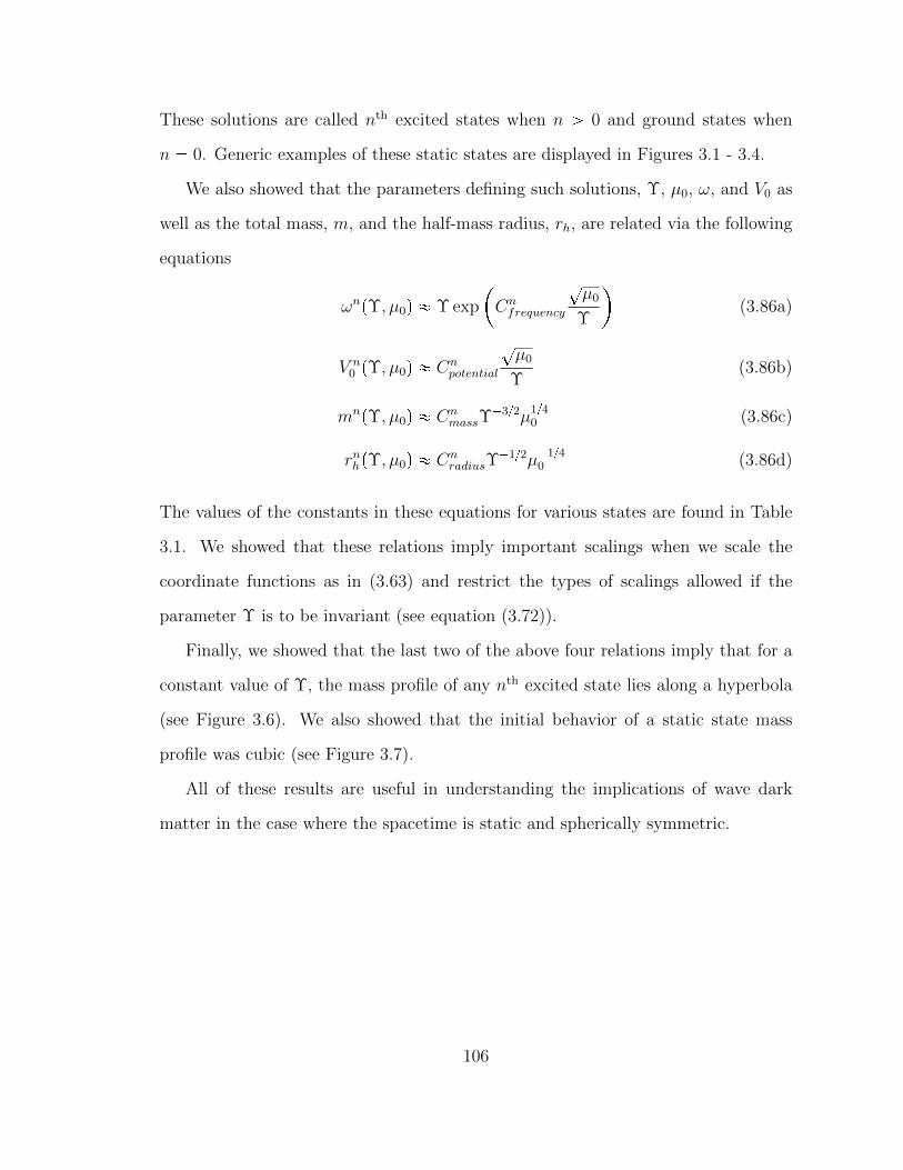
These solutions are called nth excited states when n ¡ 0 and ground states when
n 0. Generic examples of these static states are displayed in Figures 3.1 - 3.4.
We also showed that the parameters defining such solutions, Υ, µ0, ω, and V0 as
well as the total mass, m, and the half-mass radius, rh, are related via the following
equations
ωnpΥ, µ0q Υ exp
Cnfrequency
?µ0
Υ
(3.86a)
V n0 pΥ, µ0q Cn
potential
?µ0
Υ(3.86b)
mnpΥ, µ0q CnmassΥ
32µ140 (3.86c)
rnhpΥ, µ0q CnradiusΥ
12µ140 (3.86d)
The values of the constants in these equations for various states are found in Table
3.1. We showed that these relations imply important scalings when we scale the
coordinate functions as in (3.63) and restrict the types of scalings allowed if the
parameter Υ is to be invariant (see equation (3.72)).
Finally, we showed that the last two of the above four relations imply that for a
constant value of Υ, the mass profile of any nth excited state lies along a hyperbola
(see Figure 3.6). We also showed that the initial behavior of a static state mass
profile was cubic (see Figure 3.7).
All of these results are useful in understanding the implications of wave dark
matter in the case where the spacetime is static and spherically symmetric.
106

4
Modeling Wave Dark Matterin Dwarf Spheroidal Galaxies
In the last two decades, there has been substantial progress on describing the dis-
tribution of dark matter on the galactic scale. Navarro, Frenk, and White’s popular
model (Navarro et al. (1996)), which resulted from detailed N -body simulations, has
been shown to agree well with observations outside the centers of galaxies (Humphrey
et al. (2006); Walker et al. (2009)). However, the Navarro-Frenk-White dark matter
energy density profile also exhibits an infinite cusp at the origin, while observations
favor a bounded value of the dark matter energy density at the centers of galaxies
(de Blok (2010); Gentile et al. (2004)). This has prompted many astrophysicists to
employ a cored profile, such as the Burkert profile (Burkert (1995)), which “cores”
out the infinite cusp, to model the dark matter energy density in a galaxy. Resolving
this “core-cusp problem” remains an important open problem in the study of dark
matter.
Wave dark matter presents one possible solution to this problem and potentially
other astrophysical problems. In this chapter, we begin to test wave dark matter
107

against observations at the galactic level. In particular, we seek a working estimate
of the fundamental constant in the wave dark matter model, Υ, to be used in future
comparisons to data. To do so, we will compare the simplest model defined by wave
dark matter, namely the spherically symmetric static states described in the previous
chapter, to models of dark matter that are already known to fit observations well.
Salucci et al. recently used the Burkert profile to model the dark matter energy
density profiles of the eight classical dwarf spheroidal galaxies orbiting the Milky Way.
They found excellent agreement between the observed velocity dispersion profiles of
these galaxies and those velocity dispersion profiles predicted by the Burkert profile
(Salucci et al. (2012)). This can be seen in Figure 4.1, which we have reproduced
exactly as it appears in the paper by Salucci et al. In what follows, we will show that
a value of Υ 50 yr1 produces wave dark matter mass models that are qualitatively
similar to the Burkert mass models found by Salucci et al. We will also show that
under precise assumptions, comparisons to these Burkert profiles can be used to
bound the value of Υ above by 1000 yr1.
4.1 Burkert Mass Profiles
The Burkert energy density profile models the energy density of a spherically sym-
metric dark matter halo using the function
µBprq ρ0r3c
pr rcqpr2 r2c q
(4.1)
where ρ0 is the central density and rc is the core radius. Integrating this function
over the ball of radius r centered at the origin, Brp0q, with respect to the standard
108

Figure 4.1: Observed velocity dispersion profiles of the eight classical dwarf spher-oidal galaxies are denoted by the points on each plot with its associated error bars.The solid lines overlayed on these profiles are the best fit velocity dispersion profilespredicted by the Burkert mass profile. This figure is directly reproduced from thepaper by Salucci et al. (Salucci et al. (2012)) and the reader is referred to their paperfor a complete description of how these models were computed.
spherical volume form yields the Burkert mass profile as follows.
MBprq »Brp0q
µBpsq dVR3
4π
» r0
s2µBpsq ds
109

Figure 4.2: Plot of a Burkert mass profile. The inflection point is marked with an.
4π
» r0
s2ρ0r3c
ps rcqps2 r2c qds
MBprq 2πρ0r3c
ln
r rcrc
1
2ln
r2 r2
c
r2c
arctan
r
rc
(4.2)
A generic plot of a Burkert mass profile, MBprq, defined to be the dark matter mass
in the ball of radius r, is shown in Figure 4.2. We make a few remarks about the
behavior of this mass function.
Note that the behavior of the graph changes concavity at the inflection point
r rip, which we have marked on the plot in Figure 4.2 with an . Recalling
from equation (4.2) the fact that MBprq is the integral over the interval r0, rs of the
function 4πr2µBprq, we can compute this inflection point as follows.
M 1Bprq 4πr2µBprq 4πρ0r
3cr
2
pr rcqpr2 r2c q
(4.3)
Differentiating again yields
M2Bprq
4πρ0r3c pr4 r2r2
c 2rr3c q
pr rcq2pr2 r2c q2
, (4.4)
110

which has two complex zeros and two real zeros. The two real zeros are r 0 and
rip
3 p27 3?
78q233p27 3
?78q13
rc 1.52rc, (4.5)
the latter being the inflection point of the mass model.
For r " rip, the plot grows logarithmically due to the fact that the arctan term
in equation (4.2) approaches a constant value as r Ñ 8. To describe the behavior
when r ! rip, we note that the Taylor expansion of MBprq centered at r 0 is as
follows,
MBprq 4
3πρ0r
3 Opr4q. (4.6)
Thus for r ! rip, MBprq is dominated by an r3 term making the initial behavior
cubic.
In fact, several other models for dark matter mass profiles have similar initial
behavior to the Burkert profile including a quadratic mass profile (which is not
physical and is only included for the sake of comparisons) and wave dark matter
mass profiles. In Figure 4.3, we have collected several mass models that have similar
behavior inside r rip to the Burkert mass profile computed by Salucci et al. for
the Carina galaxy (Salucci et al. (2012)). While these models have similar behavior
inside r rip, they are very different outside r rip.
We have computed the inflection points of each of the Burkert mass profiles
computed by Salucci et al. for the eight classical dwarf spheroidal galaxies (Salucci
et al. (2012)) and have marked these points on a plot of each Burkert mass profile
in Figure 4.4. We have constrained the viewing window of each plot to the range
of data points collected. That is, we plot the Burkert mass profiles on the interval
r0, rlasts, where rlast is the radius of the outermost data point given by Walker et al.
(Walker et al. (2009, 2010)) for the observed velocity dispersion profiles. We have
presented them in order from greatest to least according to the ratio of rlastrip.111

Figure 4.3: Left: Plot of the Burkert mass profile for the Carina galaxy found bySalucci et al. (Salucci et al. (2012)) along with a mass plot of a wave dark matter staticground state, the cubic function which is the leading term of the Taylor expansion
of the Burkert mass profile, and the quadratic power functionMBprcqr2c
r2 where rc
is the core radius of the Carina galaxy. The marks the location of the inflectionpoint of the Burkert mass profile, while the vertical line denotes the location of theoutermost data point for the Carina galaxy and is presented for reference purposesonly. Right: Closeup of the plot on the left over the r interval r0, rips.
In Table 4.1, we have collected the defining parameters, ρ0 and rc, computed by
Salucci et al. for the Burkert mass profiles which best predict the velocity dispersion
profiles of each galaxy (Salucci et al. (2012)). We have also collected the outermost
data point, rlast, of these velocity dispersion profiles (Walker et al. (2009, 2010)),
as well as our computations of the inflection point, rip, and the ratio rlastrip for
each of the classical dwarf spheroidal galaxies. All quantities have been converted to
geometrized units (the universal gravitational constant and the speed of light set to
one) of (light)years for mass, length, and time.
4.2 Static States of Wave Dark Matter
To compare the wave dark matter model to dwarf spheroidal galaxies, we will use the
spherically symmetric static states of wave dark matter defined in Chapter 3. We will
112

Figure 4.4: Plots of the Burkert mass profiles computed by Salucci et al. of the eightclassical dwarf spheroidal galaxies within the range of observable data. The inflectionpoint is marked on each plot by an . Carina and Draco have no inflection pointmarked because the inflection point for their Burkert mass profiles occurs outsidethe range of observable data.
also take particular advantage of the property of these states that the possible mass
profiles of an nth excited state of constant Υ lie along a hyperbola. This property will
help us define a suitable definition for the nth excited state mass profile of constant Υ
that best fits a given Burkert mass profile. We do exactly this in the next subsection.
In the subsections following, we present the resulting estimates of Υ we can obtain.
113
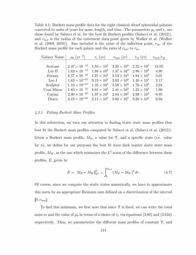
Table 4.1: Burkert mass profile data for the eight classical dwarf spheroidal galaxiesconverted to units of years for mass, length, and time. The parameters ρ0 and rc arethose found by Salucci et al. for the best fit Burkert profiles (Salucci et al. (2012)),and rlast is the radius of the outermost data point given by Walker et al. (Walkeret al. (2009, 2010)). Also included is the value of the inflection point, rip, of theBurkert mass profile for each galaxy and the ratio of rlast to rip.
Galaxy Name ρ0 (yr2) rc (yr) rlast (yr) rip (yr) rlastrip
Sextans 2.47 1014 1.53 102 3.26 103 2.32 102 14.05Leo II 1.83 1014 1.88 102 1.37 103 2.86 102 4.80Fornax 8.57 1016 1.21 103 5.54 103 1.84 103 3.01Leo I 1.83 1015 9.19 102 3.03 103 1.40 103 2.17
Sculptor 1.10 1015 1.16 103 3.59 103 1.76 103 2.04Ursa Minor 1.83 1015 8.01 102 2.41 103 1.22 103 1.98
Carina 2.90 1016 1.97 103 2.84 103 2.99 103 0.95Draco 8.19 1016 2.11 103 3.00 103 3.20 103 0.94
4.2.1 Fitting Burkert Mass Profiles
In this subsection, we turn our attention to finding static state mass profiles that
best fit the Burkert mass profiles computed by Salucci et al. (Salucci et al. (2012)).
Given a Burkert mass profile, MB, a value for Υ, and a specific state (i.e. value
for n), we define for our purposes the best fit wave dark matter static state mass
profile, MW , as the one which minimizes the L2 norm of the difference between these
profiles, E, given by
E MB MW 2L2
» rlast0
pMB MW q2 dr. (4.7)
Of course, since we compute the static states numerically, we have to approximate
this norm by an appropriate Riemann sum defined on a discretization of the interval
r0, rlasts.To find this minimum, we first note that since Υ is fixed, we can write the total
mass m and the value of µ0 in terms of a choice of rh via equations (3.80) and (3.62d)
respectively. Thus, we parameterize the different mass profiles of constant Υ, and
114
hence E by rh, that is, E Eprhq. Furthermore, since all of the static state mass
profiles of constant Υ lie on a hyperbola, there will be a value of rh that yields the
minimum of Eprhq.To make computing the best fits more uniform from galaxy to galaxy, we make
the choice rh brc, where b ¡ 0 and rc is the core radius of the Burkert profile we
wish to match, and vary the free parameter b. To compute which value of b produces
a minimum value of Eprhq, we create a grid of rh values around an initial choice of b
of the form rpb stepqrc, brc, pb stepqrcs for some step ¡ 0. Next we compute Eprhqfor each of the values of rh and shift the grid, if necessary, so that it is centered on the
rh value which yielded the smallest value of Eprhq. If the grid shifts, we recompute
Eprhq on the new grid and continue to shift, if necessary. Once the minimum Eprhqvalue occurs at the center of the grid, we keep that point as the center, but cut the
step size in half. We then run this shifting procedure again for this smaller grid until
the minimum is at the center and then we shrink again. We continue to shrink the
step size until we get to a predetermined terminal value. We generally would run
the procedure until the step size was less than or equal to 210.
In the next subsection, we will use this matching procedure to show that there
exists a value of Υ which produces similar mass profiles to those computed by Salucci
et al. (Salucci et al. (2012)). This best fitting procedure also provides a method of
finding values of Υ, for Υ sufficiently large, which produce untenable matches to the
Burkert profiles of Salucci et al. (Salucci et al. (2012)). We will explore this in more
detail in Section 4.2.3.
4.2.2 Working Value of Υ
As stated before, our overall goal is to find a value of Υ that is compatible with the
Burkert mass profiles that Salucci et al. (Salucci et al. (2012)) computed to model
the dark matter in the eight classical dwarf spheroidal galaxies. For Υ 50 yr1,
115

there is at least one wave dark matter static state that matches the Burkert mass
profiles reasonably well. We have plotted such matches in Figure 4.5. Thus we have
chosen to use
Υ 50 yr1 (4.8)
as a working value of Υ in our future work with wave dark matter until we have the
capability to make a more accurate approximation or precise measurement of this
value.
While we have chosen Υ 50 yr1 as a working value of Υ since it corresponds
to wave dark matter models compatible with other well fitting models, we note that
the above does not constitute a precise measurement of the value of Υ.
In the remainder of this chapter, we will show that, under precise assumptions, the
value of Υ can be bounded above, a first step towards obtaining a direct measurement
of Υ.
4.2.3 Upper Bound for Υ
To find an upper bound for Υ, we first need to explain how the static states change as
Υ gets large. Equation (3.80) implies that for a given nth excited state, as Υ increases,
the product mrh decreases. The hyperbolas corresponding to smaller values of mrh
are those that lie closer to the mass and radius axes.
Now consider the nth excited state mass profile that is the best fit to a Burkert
mass profile for a given Υ. As Υ increases, the hyperbola to which this static state
mass profile corresponds will get closer to the mass and radius axes, but since the
mass profile must also minimize Eprhq, the value of its total mass will not tend to
0. Since mrh tends to zero as Υ Ñ 8, it must be instead that rh Ñ 0 as Υ Ñ 8.
This implies that, as Υ increases, more of the constant portion of the best fitting nth
excited state mass profile will be compared to the Burkert profile. Thus, as Υ Ñ 8,
the best fitting nth excited state mass profile will limit to the constant function of r
116

Figure 4.5: Static state mass profiles for Υ 50 which are each a best fit to theBurkert profiles of the corresponding dwarf spheroidal galaxy. For Υ 50, we pickedan nth excited state whose best fit profile matched the Burkert profile qualitativelywell. This shows that Υ 50 is a reasonable working value of Υ. However, it doesnot imply that the actual value of Υ is 50 or that these galaxies are correctly modeledby the presented nth excited state. The units on Υ are yr1.
that best fits the Burkert profile under the same fitting criteria used for the static
states. We illustrate this phenomenon in Figure 4.6.
As Υ Ñ 8, the initial increasing region (i.e. the region before the constant
portion) of the nth excited state mass profile that best fits a Burkert mass profile
becomes more compressed. This initial region is where all of the dark matter mass
is located. Thus as Υ increases, the dark matter corresponding to the best fit nth
117

Figure 4.6: Left: Ground state mass profiles of various values of Υ that are bestfits to the Burkert mass profile found by Salucci et al. (Salucci et al. (2012)) for theLeo II galaxy. The corresponding hyperbolas of constant Υ on which these profileslie are also plotted. Ground states and their corresponding hyperbolas are drawn inthe same color. Right: The same plots as in the left frame, but with the constantfunction which best fits the Burkert profile also plotted. Note that the best fit massprofiles approach this constant mass profile as Υ increases.
excited state extends out to smaller radii. However, observations suggests that dwarf
spheroidal galaxies are dark matter dominated at all observable radii (Kleyna et al.
(2002)). Thus the best fit nth excited state mass profiles for large Υ do not represent
observations well and can be rejected. The question then is exactly when should we
reject them.
Since every static state has the initial increasing region just described, the best
fit nth excited state for any value of Υ will be a better fit than the best fit constant
function. Moreover, since this initial region becomes more compressed as Υ Ñ 8,
for large Υ, the value of Eprhq for the best fit nth excited state mass profile increases
monotonically as Υ Ñ 8 approaching the value of E for the best fitting constant
function.
This suggests a criteria for when to reject values of Υ. We will reject a best fit nth
excited state mass profile, and hence its corresponding value of Υ, as an untenable
model of the dark matter mass if its value of Eprhq is greater than some prescribed
fraction of the value of E for the best fitting constant function. We choose to use
118

80%. Explicitly, we use the following rejection criteria.
Rejection Criteria 4.2.1. Given Υ, n, and a Burkert mass profile MB, let MW be
the spherically symmetric nth excited state mass profile corresponding to Υ that best
fits MB, that is, that minimizes E from equation (4.7) along the hyperbola defined by
the value of Υ and equation (3.80). Let EW be the value of E for this mass profile.
Furthermore, let MC be the constant function which best fits MB, also by minimizing
the corresponding function E, and let EC be the value of E for the constant function.
Reject the given value Υ as a tenable value for this fundamental constant if
EW ¥ .8EC .
In other words, any fit that is less than 20% better than the best fitting constant
function of r is rejected as a bad fit.
For each of the eight dwarf spheroidal galaxies and n P t0, 1, 2, 3, 4, 5, 10, 20u, we
computed values of Υ that yielded nth excited state mass profiles that best fit that
galaxy’s Burkert profile which were rejected by the above criteria. All of the values
of Υ above those computed are also rejected because they produce mass profiles even
closer to the constant function. In Table 4.2, we have collected these upper bounds
of Υ. In Figure 4.7, for the galaxy Sextans, we present best fit static state mass
profiles for the ground through fifth, tenth, and twentieth excited states for which
Eprhq is more than 80% of the value of E for the best fit constant function.
We observe from Table 4.2 that the upper bound values of Υ increase as we
increase the state we consider. This is due to the following. The rejected values
of Υ correspond to rejected hyperbolas of constant Υ, and hence constant mrh.
Furthermore, the only qualitative difference between any two nth excited state mass
profiles is the number of ripples in the initial increasing region of the profile. For
large Υ, the majority of a best fit nth excited state mass profile that is compared to
the Burkert profile is the constant region which is shared by static state mass profiles
119

Figure 4.7: The Burkert mass profile found by Salucci et al. (Salucci et al. (2012))for the Sextans galaxy. The best fit static state mass profiles for a ground throughfifth excited state, tenth excited state, and twentieth excited state all lying on thesame hyperbola are overlayed on the plot. The hyperbola here satisfies the rejectioncriteria for all of the different static states represented in the plot, thus all of thesestatic states correspond to an upper bound on the value of Υ for Sextans for theirrespective value of n (i.e. the set of nth excited states). Note how close together allof the states are. This is due to the fact that the majority of their profiles which arebeing compared to the Burkert mass profile is the common and constant portion ofthe profiles.
for any n. Thus the hyperbola corresponding to a rejected best fit ground state is
close to the hyperbola corresponding to a rejected best fit nth excited state for any
n. In particular, there is a hyperbola of constant mrh, for which the corresponding
best fit nth excited state mass profiles for any n are rejected by the above criteria.
Then, since Cnmass and Cn
radius appear to monotonically increase as n increases (see
Table 3.1), by equation (3.80), we would expect the same behavior for the value of
Υ in order for mrh to remain constant, which is what we observe in Table 4.2.
Thus if a dwarf spheroidal galaxy is correctly modeled by a twentieth excited state
or less, then an overall upper bound on the value of Υ would be the upper bound
corresponding to the twentieth excited state. The least upper bound corresponding
to the twentieth excited state over all eight galaxies is that value for the Fornax
120

Table 4.2: Upper bound values for Υ corresponding to poor best fits of the Burkertmass profiles for each of the classic dwarf spheroidal galaxies. The values in eachcolumn for each galaxy should be interpreted as an upper bound on the value of Υ,under the approximations explained in the paper, if that galaxy is best modeled byan nth excited state. The units on Υ are yr1.
Galaxy z State 0 1 2 3
Sextans Υ 160 Υ 394 Υ 633 Υ 875Leo II Υ 234 Υ 576 Υ 926 Υ 1279Fornax Υ 35 Υ 87 Υ 139 Υ 192Leo I Υ 57 Υ 141 Υ 226 Υ 312
Sculptor Υ 49 Υ 121 Υ 194 Υ 268Ursa Minor Υ 82 Υ 202 Υ 325 Υ 449
Carina Υ 84 Υ 207 Υ 333 Υ 459Draco Υ 45 Υ 111 Υ 179 Υ 246
Galaxy z State 4 5 10 20
Sextans Υ 1116 Υ 1356 Υ 2460 Υ 4789Leo II Υ 1632 Υ 1983 Υ 3597 Υ 7003Fornax Υ 245 Υ 297 Υ 538 Υ 1048Leo I Υ 398 Υ 484 Υ 877 Υ 1706
Sculptor Υ 342 Υ 416 Υ 754 Υ 1467Ursa Minor Υ 572 Υ 695 Υ 1261 Υ 2455
Carina Υ 586 Υ 712 Υ 1292 Υ 2514Draco Υ 314 Υ 382 Υ 692 Υ 1347
galaxy, which yields approximately that
Υ 1000 yr1. (4.9)
4.2.4 Lower Bound for Υ
The next most natural goal here would be to attempt to use similar methods to
acquire a lower bound for Υ. However, it appears that no such bound could be had
without either new observations or imposing additional rather arbitrary assumptions.
This is due to the fact that as Υ decreases, the hyperbolas on which the static state
mass profiles reside would move arbitrarily far away from the axes. Thus for small Υ,
121

Figure 4.8: The Burkert mass profile found by Salucci et al.Salucci et al. (2012)for the Leo II galaxy. The best fit ground state mass profiles for successively smallervalues of Υ are overlayed on the plot. Also plotted is the best fit cubic power function,ar3, which almost coincides with the mass plot for Υ 1 and so is somewhat difficultto make out. However, it is apparent that for successively smaller values of Υ, thebest fit ground state approaches the best fit cubic function.
the initial region of the static state mass profile would dominate the part of the static
state mass profile that gets compared to the Burkert mass profile in the observable
range. Hence, for any n, as Υ Ñ 0, the best fitting nth excited state mass profile
would converge to the best fitting cubic profile since the initial region of any static
state mass profile is cubic by equation (3.83). Figure 4.8 illustrates for a ground
state this convergence to the best fitting cubic profile as Υ Ñ 0.
However, a cubic dark matter mass profile is not clearly rejectable like a constant
dark matter mass profile was. This is because a cubic profile is actually a decent fit in
the observable range for some of the Burkert profiles of the classic dwarf spheroidal
galaxies. Thus there is no way to categorically reject best fitting mass profiles of
small Υ under our current set of assumptions.
That said, we should note that as Υ Ñ 0, these static state mass profiles have the
additional property that they become arbitrarily massive and arbitrarily wide. Thus
if one could clearly bound the size of the mass or radius of the eight classical dwarf
122

spheroidal galaxies, one could obtain a lower bound on Υ by rejecting any value of
Υ which yields a dark matter halo that is too large. Unfortunately, currently we
can only detect the dark matter halo where we have stars to trace out its gravita-
tional effects or strong evidence of gravitational lensing, which makes determining
the precise overall size of the dark matter halo a very difficult undertaking.
Thus, short of making an arbitrary assumption on the size of the dark matter
halos surrounding these dwarf spheroidal galaxies, we either must wait for bounds
on the size of the halos to be observed or find another method of determining a lower
bound.
4.3 Utilized Approximations
Now that we have presented our results, we list here the important approximations
made in this chapter which led to these results and explain briefly why we make
them.
Approximation 1: Dark matter is correctly described by the wave dark matter
model.
Approximation 2: Dark matter halos around dwarf spheroidal galaxies are spher-
ically symmetric.
Approximation 3: The dwarf spheroidal galaxies used in this chapter are in a state
of dynamical equilibrium.
Approximation 4: The spacetime metrics describing these dwarf spheroidal galax-
ies are static.
Approximation 5: Wave dark matter predicts outcomes qualitatively similar to
those of spherically symmetric static state solutions to the Einstein-Klein-
Gordon equations.
123

Approximation 6: The Burkert mass profiles computed by Salucci et al. (Salucci
et al. (2012)) fit the observational data very well.
Approximation 7: The spacetime is in the low field limit, that is, M ! r.
Approximation 8: The spacetime is asymptotically Schwarzschild.
Approximation 1 is used because we are testing the wave dark matter model
against observations. Approximation 2 is a common approximation for dwarf spher-
oidal galaxies and is also necessary because we are comparing the wave dark matter
model to the spherically symmetric Burkert mass profile. Approximation 3 seems
to be consistent with observations of dwarf spheroidal galaxies at least out to large
radii (Salucci et al. (2012); Cote et al. (1999)). Approximation 6 is reasonable given
Figure 4.1. Approximations 7 and 8 are standard when modeling galaxies.
Approximations 4 and 5 are used to simplify the types of solutions to the Einstein-
Klein-Gordon equations we consider. We note here, however, that there is a question
of the stability of the spherically symmetric static state solutions. It is known that,
if the corresponding total mass is not too large, the ground state is stable under
perturbations (Seidel and Suen (1990); Lai and Choptuik (2007)) but that, on their
own, the excited states are not (Balakrishna et al. (1998)) regardless of their mass.
However, it has also been shown that a coupling of an excited state with a ground
state can produce a stable configuration (Bernal et al. (2010)). We hypothesize that
luminous matter distributions coupled with combinations of static states will produce
a stabilizing effect allowing for more dynamically interesting systems to be physically
plausible.
4.4 Conclusions
To summarize the results of this paper, we have drawn effectively two conclusions,
which we list here.
124

Conclusion 4.4.1. Given Approximations 1 through 8, a value of Υ which yields
one or more spherically symmetric static state mass profiles which match well the
best fit Burkert mass profiles computed by Salucci et al. (Salucci et al. (2012)) for
each of the eight classical dwarf spheroidal galaxies is
Υ 50 yr1.
Conclusion 4.4.2. Given Approximations 1 through 8 and Rejection Criteria 4.2.1,
if the dark matter halos of all of the eight classical dwarf spheroidal galaxies are
correctly modeled by 20th excited states or less, then
Υ 1000 yr1.
For the interested reader, the Matlab code used for this dissertation to generate
the spherically symmetric static states and to compute the best fits to a Burkert
profile can be found on Bray’s Wave Dark Matter Web Page at http://www.math.
duke.edu/~bray/darkmatter/darkmatter.html.
125

5
A Numerical Scheme to Solve theEinstein-Klein-Gordon Equations
in Spherical Symmetry
In this chapter, we present some of the progress we have made on the next part of
our research into wave dark matter and dwarf spheroidal galaxies. The next project
we are interested in is numerically solving the Einstein-Klein-Gordon equations in
spherical symmetry in order to determine more generic solutions to these equations
and perhaps use these equations to obtain a better estimate of Υ. Thus far, we have
designed numerical code to evolve these equations, but there is still much to do in
terms of analyzing the practical properties of the scheme and conducting experiments
to generate generic solutions.
This chapter presents the numerical scheme we use to solve the spherically sym-
metric Einstein-Klein-Gordon equations. We will discuss how to appropriately imple-
ment the boundary conditions into the scheme as well as some artificial dissipation.
We will also discuss the accuracy and stability of the scheme. Finally, we will present
some examples that show the scheme in action and illustrate how to use the code.
126

We wish to numerically evolve the spherically symmetric Einstein-Klein-Gordon
equations found in equation (2.58). The boundary conditions on these equations at
r 0 are found in equations (3.3), (3.4), and (3.6). These boundary conditions allow
us to compute equation (2.58) at r 0 by taking the limit as r Ñ 0, which yields
Mrpt, 0q 0 (5.1a)
Vrpt, 0q 0 (5.1b)
ftpt, 0q ppt, 0qeV pt,0q (5.1c)
ptpt, 0q eV pt,0q3frrpt, 0q Υ2fpt, 0q . (5.1d)
The above conditions on the central values are necessary for regularity at r 0
and so will always hold in the low field limit. As in the case of the static states,
even though theoretically we consider an infinite spacetime, to compute numerical
solutions to these equations we must set an artificial right hand boundary point and
impose boundary conditions. If r rmax is the maximum r value included in the
computation, then we will require as a boundary condition that
ppt, rmaxq frpt, rmaxq λpppt, rmaxq frpt, rmaxqq, (5.2)
for some λ P C and |λ| ¤ 1. This splits into three cases, λ 1, λ 1, and λ 1.
If λ 1, then we have that
frpt, rmaxq 0, (5.3)
which is a Neumann boundary condition. If λ 1, then we have that
ppt, rmaxq 0 and hence fpt, rmaxq fp0, rmaxq (5.4)
for all t. This is a Dirichlet boundary condition. If λ is any other complex number,
then we will have that
frpt, rmaxq λ 1
λ 1
ppt, rmaxq. (5.5)
127

This boundary condition has a physical interpretation. Given the metric, the
future-pointing null vectors in the radial direction are
EO eV Bt c
1 2M
rBr, (5.6)
EI eV Bt c
1 2M
rBr. (5.7)
Then equation (5.2) is a simplification of the following equation
EOpfq|rrmax λEIpfq|rrmax
eV ft c
1 2M
rfr
rrmax
λ
eV ft
c1 2M
rfr
rrmax
eV
1 2M
r
12ft fr
rrmax
λ
eV
1 2M
r
12ft fr
rrmax
ppt, rmaxq frpt, rmaxq λpppt, rmaxq frpt, rmaxqq (5.8)
Since EOpfq is the outward null derivative, it is the change of f along a light ray
leaving the system. Since we are measuring the change along a light ray which moves
faster than any amount of scalar field exiting the system, the only flux EOpfq can
detect is the amount of scalar field moving into the system. Similarly, EIpfq is the
inward null derivative and by the same reasoning can only detect the amount of
scalar field moving out of the system. This idea is displayed pictorially in Figures
5.1 and 5.2. Thus the boundary condition in equation (5.2) can be interpreted as
the amount of matter that is flowing into the system is some multiple of the amount
of matter that is flowing out. The parameter λ controls how much matter is sent
back in. Since λ can be any complex number with absolute value less than one, it
can also phase shift the scalar field it sends back in.
An image that might help make this more clear, is that we have set up a sort
of mirror on the outside boundary, where the level of reflectivity is controlled by λ,
128

t t0 dt
f
f
t t0
EOrmax
rmax
Figure 5.1: Image of an incoming and outgoing wave at the boundary rmax. Thefuture pointing outward null vector EO is also displayed. Since no outgoing wave cantravel faster than the speed of the null vector shown, then computing the change off along this null vector will only detect changes in f due to incoming waves.
t t0 dt
f
f
t t0
rmax
rmax
EI
Figure 5.2: Image of an incoming and outgoing wave at the boundary rmax. Thefuture pointing inward null vector EI is also displayed. Since no incoming wave cantravel faster than the speed of the null vector shown, then computing the change off along this null vector will only detect changes in f due to outgoing waves.
which we will call the reflectivity constant. For example, for a value of λ 1, all
outgoing waves are immediately replaced by incoming waves of the same amplitude
and phase. Restricting the viewing window to the left of the r rmax boundary
shows that this is equivalent to the outgoing wave reflecting back in exactly as it
left with the same phase. This is depicted in Figure 5.3. For a value of λ 1, all
outgoing waves are immediate replaced by incoming waves of the same amplitude
but opposite phase (i.e. all of the peaks of the outgoing wave correspond to valleys
of the incoming wave and vice versa). Again, restricting the viewing window to the
129

rmax
f
f
f
t
Figure 5.3: A depiction of what is simulated by the boundary condition (5.2) withλ 1. In this case, all outgoing waves are replaced by incoming waves of the sameamplitude and phase. If we restrict our attention to the left of the vertical dottedline representing r rmax, we see that this is equivalent to the outgoing wave beingimmediately reflected by the boundary back into the system with the same amplitudeand phase. All values of λ in the boundary condition (5.2) can be interpreted as someamplifying or damping phase-shifting reflection.
left of the r rmax boundary shows that this is equivalent to the outgoing wave
being reflected back in with the opposite phase. This is depicted in Figure 5.4. Any
value of λ for which |λ| 1 will preserve the total mass at the right hand boundary.
Values of λ with |λ| 1 will allow the mass to decrease at the boundary but not
increase, as it lets out more mass than it reflects back in. Values of λ will |λ| ¡ 1 will
allow the mass to increase at the boundary but not decrease, as it “reflects” more
mass in than it lets out. A value of λ 0 is the absence of any reflectivity, so things
can only leave the system with nothing entering. As is expected, we could use this
boundary condition to simulate matter being artificially added to the system, but
for the intents here, we only wish to allow the possibility that the amount reflected
back in is bounded above by the amount that leaves the system. Hence the condition
mentioned before that |λ| ¤ 1.
130

rmax
f
f
t
f
f
Figure 5.4: A depiction of what is simulated by the boundary condition (5.2) withλ 1. In this case, all outgoing waves are replaced by incoming waves of thesame amplitude, but opposite phase (i.e. all peaks are valleys and vice versa). If werestrict our attention to the left of the vertical dotted line representing r rmax, wesee that this is equivalent to the outgoing wave being immediately reflected by theboundary back into the system with the same amplitude, but opposite phase. Allvalues of λ in the boundary condition (5.2) can be interpreted as some amplifying ordamping phase-shifting reflection.
Now that we have described the setup of the PDEs we wish to solve, we can
discretize the system and apply a numerical scheme to solve it.
5.1 The Numerical Scheme
We will solve this system in two steps. Given consistent initial conditions, we will
first evolve equations (2.58c) and (2.58d) a single step in time and then compute
the compatible metric components M and V using the system of ODEs (2.58a) and
(2.58b).
Since the system (2.58c) and (2.58d) is first order in time, we will solve it using the
131

method of lines. This entails discretizing every spatial derivative and then solving the
resulting system of ODEs in time using a standard ODE technique. In this case, we
will discretize the spatial derivatives using the standard second order centered finite
difference and then use the third order Runge-Kutta method (Gottlieb et al. (2001);
Alic et al. (2007)), which is stable so long as the usual CFL condition is satisfied, to
evolve in time. For purposes of smoothing and to dissipate any high oscillation noise
that may occur, we will also add in artificial Kreiss-Oliger dissipation (Kreiss and
Oliger (1973); Lai (2004)) after each full Runge-Kutta time step. While how these are
implemented in our problem will all be described below in detail, for convenience, we
will write down the forward Euler discretization of a first derivative in time, forward
Euler of a first derivative in space, and second order centered finite difference of
both a first and second derivative in space on a mesh ptn, rkq for a function f , where
fnk fptn, rkq. We have that
Forward Euler in Time: pftqnk fn1k fnk
∆t
Forward Euler in Space: pfrqnk fnk1 fnk
∆r
2nd Order Center FD in space: pfrqnk fnk1 fnk1
2∆r,
pfrrqnk fnk1 2fnk fnk1
p∆rq2
After each complete partial time step, we will recompute the corresponding met-
ric using a modified forward Euler scheme to solve the spatial ODEs (2.58a) and
(2.58b) at the current time. This is the method we will follow to update the metric
components at each step.
Now we will setup the discretization. We will compute everything in terms of r
and t. Let the computational domain be r0, rmaxs. Then we will discretize this into
132
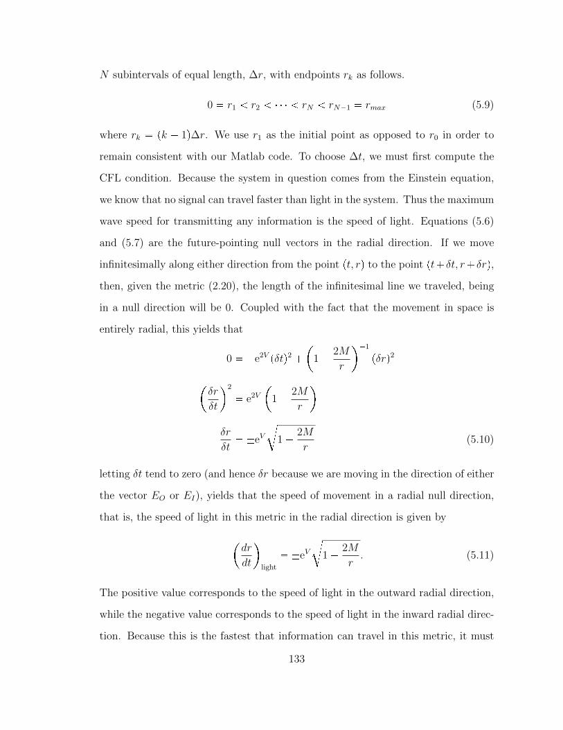
N subintervals of equal length, ∆r, with endpoints rk as follows.
0 r1 r2 rN rN1 rmax (5.9)
where rk pk 1q∆r. We use r1 as the initial point as opposed to r0 in order to
remain consistent with our Matlab code. To choose ∆t, we must first compute the
CFL condition. Because the system in question comes from the Einstein equation,
we know that no signal can travel faster than light in the system. Thus the maximum
wave speed for transmitting any information is the speed of light. Equations (5.6)
and (5.7) are the future-pointing null vectors in the radial direction. If we move
infinitesimally along either direction from the point pt, rq to the point pt δt, r δrq,then, given the metric (2.20), the length of the infinitesimal line we traveled, being
in a null direction will be 0. Coupled with the fact that the movement in space is
entirely radial, this yields that
0 e2V pδtq2
1 2M
r
1
pδrq2
δr
δt
2
e2V
1 2M
r
δr
δt eV
c1 2M
r(5.10)
letting δt tend to zero (and hence δr because we are moving in the direction of either
the vector EO or EI), yields that the speed of movement in a radial null direction,
that is, the speed of light in this metric in the radial direction is given by
dr
dt
light
eVc
1 2M
r. (5.11)
The positive value corresponds to the speed of light in the outward radial direction,
while the negative value corresponds to the speed of light in the inward radial direc-
tion. Because this is the fastest that information can travel in this metric, it must
133

be the maximum wave speed of the equations above, which model the metric. Thus
in order for our discretization to not lose information and remain stable, we must
update before information from one mesh point can travel to the either neighboring
mesh point on the next time step. In other words, the mesh speed, ∆r∆t, must be
greater than the absolute value of the maximum wave speed, |pdrdtqlight|. This is
known as the CFL condition and is given in this case by
∆r
∆t¥ max
r,t
dr
dt
light
maxr,t
eVc
1 2M
r
∆t ¤ min
r,t
eV
1 2M
r
12∆r. (5.12)
Note that since we have to pick a ∆t in order to compute V and M and at any given
time, we can’t choose a ∆t that is guaranteed to always be smaller than the CFL
condition. To deal with this, we will make a significantly smaller choice than the
CFL condition on the initial conditions and keep the option open that if stability
issues arise, we can make an even smaller choice. Explicitly, we will choose a c ¥ 1
and define
∆t
1
c
minr
eV
1 2M
r
12∆r (5.13)
where the V and M here are the initial (t 0) values of V and M . Then we discretize
t as follows,
0 t0 t1 tn (5.14)
where tn n∆t. We can solve the equations out as far out as we desire, say tmax,
but since we have made the choice (5.13), we will actually stop at the smallest tk
value that is greater than or equal to tmax.
Now that we have defined the mesh, we can now discretize the system. First,
note that for any function, f , on the mesh, we will define fnk as the approximation
134

of the point fptn, rkq. We will first apply the above mentioned schemes to f and
p, however, since the third order Runge-Kutta is an iteration using forward Euler
steps, we will first compute only a single forward Euler step on f . Using forward
Euler for the time derivatives and second order centered finite differences for the
space derivatives, away from the boundaries, equation (2.58c) becomes
fn1k fnk
∆t pnkeV
nk
c1 2Mn
k
rk
fn1k fnk ∆tpnkeV
nk
c1 2Mn
k
rk. (5.15)
To discretize (2.58d), we first note that by (2.58a) and (2.58b), we have
Br
eV fr
c1 2M
r
Vre
V fr
c1 2M
r eV frr
c1 2M
r
eV fr
1 2M
r
12M
r2 Mr
r
eV
frr
c1 2M
r
2fr
1 2M
r
12M
r2 4πrµ0 |f |2
(5.16)
This makes (2.58d) become
pt eV
1 2M
r
122fr
M
r2 4πrµ0 |f |2
Υ2f
c
1 2M
r
frr 2fr
r
(5.17)
135

which, away from the boundaries, discretizes as
pn1k pnk
∆t eV
nk
c1 2Mn
k
rk
fnk1 2fnk fnk1
p∆rq2 fnk1 fnk1
rk∆r
1 2Mnk
rk
122
Mn
k
r2k
4πrk µ0 |fnk |2
fnk1 fnk1
2∆r
Υ2fnk
pn1k pnk ∆teV
nk
c1 2Mn
k
rk
fnk1 2fnk fnk1
p∆rq2 fnk1 fnk1
rk∆r
1 2Mnk
rk
122
Mn
k
r2k
4πrk µ0 |fnk |2
fnk1 fnk1
2∆r
Υ2fnk
(5.18)
To deal with updating the central (r 0) values of these functions, we use the
system (5.1) and (3.6). Then using our finite difference formulas at r 0, we have
that
fn2 fn1
2∆r 0 (5.19)
where fn1 is the approximation of fptn,∆rq (recall that fn1 fptn, 0q and there is
no fn0 ). This implies that fn1 fn2 . Using this fact we have that at r r1 0,
pfrrqn1 fn2 2fn1 fn1
p∆rq2 2 pfn2 fn1 qp∆rq2 . (5.20)
Then by (5.1), we get that f and p update as follows
fn11 fn1
∆t pn1 eV
n1
fn11 fn1 ∆tpn1 eV
n1 (5.21)
136

and
pn11 pn1
∆t eV
n1
6 pfn2 fn1 qp∆rq2 Υ2fn1
pn11 pn1 ∆teV
n1
6 pfn2 fn1 qp∆rq2 Υ2fn1
(5.22)
At the right hand boundary, we have to impose one of the boundary conditions,
which one depends on the choice of λ. We will treat each one individually. First, if
λ 1, equation (5.3) holds and discretizes as
fN2 fN2∆r
0 (5.23)
or that fN2 fN . Applying this to the discretizations for f and p, (5.15) and (5.18)
respectively, yields at r rN1 rmax that
fn1N1 fnN1 ∆t pnN1 eV
nN1
d1 2Mn
N1
rN1
(5.24)
and
pn1N1 pnN1 ∆t eV
nN1
Υ2fnN1
1 2Mn
N1
rN1
12
2
d1 2Mn
N1
rN1
fnN fnN1
p∆rq2
(5.25)
Next, if λ 1, then equation (5.4) holds and we don’t have to evolve anything at
the boundary. Instead, we have that for all n,
fn1N1 fnN1 (5.26)
pn1N1 0 (5.27)
Finally, if λ 1, we have equation (5.5), which yields
fnN2 fnN2∆r
λ 1
λ 1
pnN1
fnN2 fnN 2∆r pnN1
λ 1
λ 1
. (5.28)
137

Applying this to the discretizations for f and p, (5.15) and (5.18) respectively, yields
at r rN1 rmax that
fn1N1 fnN1 ∆t pnN1 eV
nN1
d1 2Mn
N1
rN1
(5.29)
and
pn1N1 pnN1 ∆t eV
nN1
1 2Mn
N1
rN1
122
Mn
N1
r2N1
4πrN1 µ0
fnN1
2λ 1
λ 1
pnN1 Υ2fnN1
2
d1 2Mn
N1
rN1
fnN fnN1
p∆rq2 pnN1
1
rN1
1
∆r
λ 1
λ 1
(5.30)
To summarize, given that we know f , p, V , and M on the time step t tn, we
evolve f and p a single forward Euler step in time as follows. At r r1 0, we have
from (5.21) and (5.22)
fn11 fn1 ∆tpn1 eV
n1 (5.31)
pn11 pn1 ∆teV
n1
6 pfn2 fn1 qp∆rq2 Υ2fn1
. (5.32)
For k 2, . . . , N , we have from (5.15) and (5.18)
fn1k fnk ∆tpnkeV
nk
c1 2Mn
k
rk(5.33)
pn1k pnk ∆teV
nk
1 2Mn
k
rk
122
Mn
k
r2k
4πrk µ0 |fnk |2
fnk1 fnk1
2∆r
Υ2fnk
c
1 2Mnk
rk
fnk1 2fnk fnk1
p∆rq2 fnk1 fnk1
rk∆r
. (5.34)
138
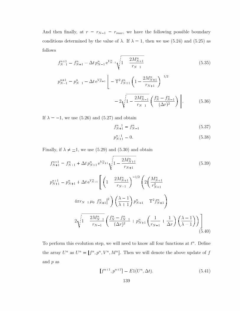
And then finally, at r rN1 rmax, we have the following possible boundary
conditions determined by the value of λ. If λ 1, then we use (5.24) and (5.25) as
follows
fn1N1 fnN1 ∆t pnN1 eV
nN1
d1 2Mn
N1
rN1
(5.35)
pn1N1 pnN1 ∆t eV
nN1
Υ2fnN1
1 2Mn
N1
rN1
12
2
d1 2Mn
N1
rN1
fnN fnN1
p∆rq2
. (5.36)
If λ 1, we use (5.26) and (5.27) and obtain
fn1N1 fnN1 (5.37)
pn1N1 0. (5.38)
Finally, if λ 1, we use (5.29) and (5.30) and obtain
fn1N1 fnN1 ∆t pnN1 eV
nN1
d1 2Mn
N1
rN1
(5.39)
pn1N1 pnN1 ∆t eV
nN1
1 2Mn
N1
rN1
122
Mn
N1
r2N1
4πrN1 µ0
fnN1
2λ 1
λ 1
pnN1 Υ2fnN1
2
d1 2Mn
N1
rN1
fnN fnN1
p∆rq2 pnN1
1
rN1
1
∆r
λ 1
λ 1
(5.40)
To perform this evolution step, we will need to know all four functions at tn. Define
the array Un as Un rfn, pn, V n,Mns. Then we will denote the above update of f
and p as
rfn1, pn1s E1pUn,∆tq. (5.41)
139

After performing that evolution step, we will need to compute the corresponding
V andM . We will write here the discretizations of equations (2.58a) and (2.58b). Un-
fortunately, due to the fact that V doesn’t appear on the right-hand side of (2.58b),
using the second order centered finite difference approximation for Vr produces a
decoupling of the even and odd discretizations points, sometimes called a “checker-
board instability”. In order to remedy this, we will used a modified forward Euler
scheme that uses both Vr and Vrr to compute the next point of V . To do this, we
will simply use the Taylor series of V truncated at the second derivative to compute
Vk1 from points at rk as follows,
Vk1 Vk pVrqk ∆r pVrrqk ∆r2
2. (5.42)
To be consistent, we will compute the points of M using the same scheme as above,
but we will continue to use the centered finite differences to approximate the space
derivatives of f and p. This should keep the overall scheme roughly second order
accurate in space.
In order to follow this overall scheme, we will have to compute formulas for Mrr
and Vrr and compute their values at r 0. To that end, we simply compute the
derivatives of equations (2.58a) and (2.58b) and obtain
Mrr 2Mr
r
1 4πr2µ0
|fr|2 |p|2
Υ2
4πr2µ0
#2 Repfrfq 2M
r2
|fr|2 |p|2
Υ2
2
1 2M
r
Repfrrfr prpq
Υ2
+(5.43)
140

Vrr
1 2M
r
1#Mr
r
1
r 2Vr 8πrµ0
|fr|2 |p|2
Υ2
Vrr
1 4M
r
3M
r3 4πrµ0
2 Repfrfq
2
1 2M
r
Repfrrfr prpq
Υ2 2M
r2
|fr|2 |p|2
Υ2
+(5.44)
There is no need, in general, to substitute in the values for Mr and Vr since we will
need to compute the values of each at every point and so can just use those values
here. Now, at r 0, we already know that
M 0, Mr 0, Mrr 0, and Vr 0. (5.45)
So we already have enough information to compute M2 Mp∆rq, and we only
need to know V and Vrr at the origin in order to have the information necessary to
compute the point V2 V p∆rq.We want V and M to define a metric that is asymptotically Schwarzschild as
with the static states. We will impose the asymptotically Schwarzschild condition at
r rmax. Thus V p0q must be chosen to satisfy (3.9) on the boundary. Note also that
given the system (2.58), for a given f and p, if M and V satisfy (2.48) and (2.50),
then so do M and V b for some constant b P R. This allows us to set V p0q 0 to
initially solve for V , followed by setting b as follows
b 1
2ln
1 2Mpt, rmaxq
rmax
lnκ V pt, rmaxq 1
2ln
1 2Mn
N1
rN1
lnκ V n
N1,
(5.46)
where as before, for convenience, we set κ 1. We will then relabel V b as simply
V . Thus for the intents and purposes of computing V at r 0, we will set V p0q 0,
imposing the right hand boundary condition after computing V and M completely.
141

For Vrr, if we attempt to take the limit of (5.44) as r Ñ 0, by L’Hopital’s Rule,
we will acquire no new information. However, if we rewrite the following
Vrr
1 4M
r
Vr
r
1 2M
r
2VrM
r
M
r3 4πµ0
|f |2
1 2M
r
|fr|2 |p|2Υ2
2VrM
r, (5.47)
then we get the equation
Vrr
1 2M
r
1#Mr
r
1
r 2Vr 8πrµ0
|fr|2 |p|2
Υ2
2VrM
r 2M
r3 4πµ0
|f |2 |fr|2 |p|2
Υ2
4πrµ0
2 Repfrfq 2
1 2M
r
Repfrrfr prpq
Υ2
+. (5.48)
In this case, we get something useful from the limit at r Ñ 0. By L’Hopital’s rule,
we obtain
limrÑ0
Vrr limrÑ0
1 2M
r
1#Mr
r
1
r 2Vr 8πrµ0
|fr|2 |p|2
Υ2
2VrM
r 2M
r3 4πµ0
|f |2 |fr|2 |p|2
Υ2
4πrµ0
2 Repfrfq 2
1 2M
r
Repfrrfr prpq
Υ2
+
limrÑ0
Mr
r2 2M
r3 4πµ0
|f |2 |p|2
Υ2
limrÑ0
Mrr
2r 2Mr
3r2 4πµ0
|f |2 |p|2
Υ2
limrÑ0
Mrrr
2 2Mrr
6r 4πµ0
|f |2 |p|2
Υ2
142

limrÑ0
Mrrr
2 Mrrr
3 4πµ0
|f |2 |p|2
Υ2
Mrrr
6 4πµ0
|f |2 |p|2
Υ2
r0
(5.49)
Now, while we don’t have enough information to pin down Mrrr at the central value
exactly, due to the fact that (2.58a) and (5.43) do not depend directly on the values
of V , we will first compute M2 Mp∆rq and M3 Mp2∆rq and then use a second
order centered finite difference formula to approximate Mrrr at r 0. Then, because
M is an odd function, we obtain
Mrrrp0q Mp2∆rq 2Mp∆rq 2Mp∆rq Mp2∆rq2p∆rq3
2Mp2∆rq 4Mp∆rq2p∆rq3
Mp2∆rq 2Mp∆rqp∆rq3
M3 2M2
p∆rq3 (5.50)
And since
M2 M1 pMrq1∆r pMrrq1 p∆rq2
2M1 0 (5.51)
we have that
Mrrrp0q M3
p∆rq3 . (5.52)
and hence
Vrrp0q pVrrq1 M3
6p∆rq3 4πµ0
|f1|2 |p1|2
Υ2
(5.53)
This gives us enough information to compute M and V near the left hand boundary
r 0, which in turn, because the scheme is explicit, gives us the necessary informa-
tion to continue the approximation out to our right hand boundary r rmax. Then
143

we only need to ensure that we have the appropriate asymptotic behavior, which we
accomplish by selecting the appropriate value b to add to the metric V , where b is
as defined in equation (5.46).
We now solve for V and M as follows; note that since all of the values will be
defined at the same tn point, we will omit the superscripts n from these equations.
At r r1 0, we have
M1 0 (5.54)
V1 0. (5.55)
Next, since Mrp0q Mrrp0q 0, we have that
M2 M1 0, (5.56)
but, as stated before, we first need to compute M3 before we can compute V2. To
compute M3, we have that
pMrq2 4πr22 µ0
|f2|2
1 2M2
r2
|f3 f1|24Υ2p∆rq2
|p2|2Υ2
(5.57)
pMrrq2 2pMrq2r2
1 4πr2
2 µ0
|f3 f1|24Υ2p∆rq2
|p2|2Υ2
4πr22 µ0
#2 Re
f3 f1
2∆r
f2
2M2
r22
|f3 f1|24Υ2p∆rq2
|p2|2Υ2
2
Υ2
1 2M2
r2
Re
f3 2f2 f1
p∆rq2
f3 f1
2∆r
p3 p1
2∆r
p2
+
(5.58)
Then we compute M3 as follows
M3 M2 pMrq2 ∆r pMrrq2 p∆rq2
2. (5.59)
144

Then we compute V2 as follows.
pVrq1 0 (5.60)
pVrrq1 M3
6p∆rq3 4πµ0
|f1|2 |p1|2
Υ2
(5.61)
which yields
V2 V1 pVrq1 ∆r pVrrq1 p∆rq2
2. (5.62)
To get V3, we have
pVrq2
1 2M2
r2
1M2
r22
4πr2 µ0
|f2|2
1 2M2
r2
|f3 f1|24Υ2p∆rq2
|p2|2Υ2
(5.63)
pVrrq2
1 2M2
r2
1#pMrq2r2
1
r2
2pVrq2 8πr2 µ0
|f3 f1|24Υ2p∆rq2
|p2|2Υ2
pVrq2r2
1 4M2
r2
3M2
r32
4πr2 µ0
2 Re
f3 f1
2∆r
f2
2
Υ2
1 2M2
r2
Re
f3 2f2 f1
p∆rq2
f3 f1
2∆r
p3 p1
2∆r
p2
2M2
r22
|f3 f1|24Υ2p∆rq2
|p2|2Υ2
+(5.64)
which yields
V3 V2 pVrq2 ∆r pVrrq2 p∆rq2
2. (5.65)
Then for k 3, . . . , N , we compute the following
pMrqk 4πr2k µ0
|fk|2
1 2Mk
rk
|fk1 fk1|24Υ2p∆rq2 |pk|2
Υ2
(5.66)
145

pMrrqk 2pMrqkrk
1 4πr2
k µ0
|fk1 fk1|2
4Υ2p∆rq2 |pk|2Υ2
4πr2k µ0
#2 Re
fk1 fk1
2∆r
fk
2Mk
r2k
|fk1 fk1|2
4Υ2p∆rq2 |pk|2Υ2
2
Υ2
1 2Mk
rk
Re
fk1 2fk fk1
p∆rq2
fk1 fk1
2∆r
pk1 pk1
2∆r
pk
+(5.67)
pVrqk
1 2Mk
rk
1Mk
r2k
4πrk µ0
|fk|2
1 2Mk
rk
|fk1 fk1|24Υ2p∆rq2 |pk|2
Υ2
(5.68)
pVrrqk
1 2Mk
rk
1#pMrqkrk
1
rk 2pVrqk 8πrk µ0
|fk1 fk1|2
4Υ2p∆rq2 |pk|2Υ2
pVrqkrk
1 4Mk
rk
3Mk
r3k
4πrk µ0
2 Re
fk1 fk1
2∆r
fk
2
Υ2
1 2Mk
rk
Re
fk1 2fk fk1
p∆rq2
fk1 fk1
2∆r
pk1 pk1
2∆r
pk
2Mk
r2k
|fk1 fk1|2
4Υ2p∆rq2 |pk|2Υ2
+(5.69)
and obtain
Mk1 Mk pMrqk ∆r pMrrqk p∆rq2
2(5.70)
Vk1 Vk pVrqk ∆r pVrrqk p∆rq2
2(5.71)
Finally, we compute b according to equation (5.46) and redefine the entire array V
as V b.
146

To perform the above update of M and V , we will only have to know the updated
values of f and p computed in E1 (from (5.41)). Since it only depends on the f and
p at any given time, we will denote this process as
rfn, pn, V n,Mns E2pfn, pnq (5.72)
Composing the two processes, E1 and E2 (from (5.41) and (5.72) respectively),
together we obtain a process of updating all four functions a single forward Euler
step in time, which we will call simply EpUn,∆tq. Explicitly, we write
Un1 rfn1, pn1, V n1,Mn1s EpUn,∆tq E2pE1pUn,∆tqq (5.73)
Now we have enough to describe in simple terms the entire process of evolving
the four functions f, p, V,M . We start with given initial conditions f 0 and p0 which
can be freely defined. Then we perform the following process.
1. Compute the compatible initial values of the metric, V 0 and M0, using E2.
That is,
U0 E2pf 0, p0q. (5.74)
2. Use the third order Runge-Kutta method (Gottlieb et al. (2001); Alic et al.
(2007)) as follows to evolve the four functions, f, p, V,M a single time step
from tn to tn1. This is a three step iterative process of successive weighted
averages of the four input functions and a forward Euler step. Explicitly, we
compute Un1 as follows.
U EpUn,∆tq (5.75a)
U 3
4Un 1
4EpU,∆tq (5.75b)
Un1 1
3Un 2
3EpU,∆tq. (5.75c)
147

3. Apply Kreiss-Oliger dissipation (Kreiss and Oliger (1973); Lai (2004)) to the
updated functions f and p as follows. This adds a smoothing factor that is
dependent on the previous time step which removes some of the high frequency
oscillation that can occur due to numerical errors. We only add this in for
k 3, . . . , N 1, the other points we leave unchanged.
fn1k fn1
k ε
16
fnk2 4fnk1 6fnk 4fnk1 fnk2
(5.76a)
pn1k pn1
k ε
16
pnk2 4pnk1 6pnk 4pnk1 pnk2
(5.76b)
where, for stability, 0 ¤ ε 1 (Kreiss and Oliger (1973); Lai (2004)) (ε 0
corresponds to no dissipation). In our case, we choose ε 12. We choose that
value for two reasons. First, this value is the typical one used (Lai (2004)).
And second, in a few trial simulations we performed of a simpler PDE where
the solution was known, this value of ε had the desired smoothing effect but
the lowest mean error when compared to other attempted values of ε including
ε 0.
4. Since we have once again changed the values of f and p, we need to once again
compute the compatible metric components V and M . Thus we apply E2
again and obtain
Un1 E2pfn1, pn1q (5.77)
5. Repeat steps 2 - 4 until the desired time value tmax is reached.
5.2 Stability and Accuracy of the Scheme
In this section, we make a few comments about the stability and accuracy of the
numerical scheme presented above.
148

5.2.1 Stability of the Scheme
We have already noted that the third order Runge-Kutta scheme is stable so long as
the CFL condition in equation (5.12) is satisfied. Moreover, the implementation of
Kreiss-Oliger dissipation is stable so long as the ε in equation (5.76) is positive and
less than one. We used ε 12 and so we should expect stability from this aspect of
the scheme. These stability results are consistent with our initial runs of the scheme
which show stable behavior for hundreds or even thousands of periods of static states
in time.
However, we did find experimentally an additional stability concern due to the
right hand boundary condition involving the reflectivity constant λ. Due to the last
term in equation (5.30), which is used whenever λ 1, we have that, since all of the
other values are generally very close to zero due to the asymptotically Schwarzschild
condition, the values of pn1N1 will progressively get larger whenever
2pnN1
eV
nN1
d1 2Mn
N1
rN1
∆t
∆r
λ 1
λ 1
2pftqnN1
∆t
∆r
λ 1
λ 1
¥ pftqnN1
(5.78)
This depends on the speed of the mesh ∆r∆t and hence is mesh-dependent and not
an effect inherent in the pdes. Due to the growing values of pn1N1 and hence fn1
N1,
if the above condition is not satisfied, the numerical scheme will be unstable at the
right hand boundary which will quickly propagate to the rest of the system. Thus
the scheme is only stable so long as the above condition with the opposite inequality
is satisfied. That is, when λ 1
λ 1
∆r
2∆t(5.79)
The term ∆r∆t occurs in the CFL condition. The CFL condition we use in practice
is found in equation (5.12) and implies that the above equation makes the above
149

inequality become λ 1
λ 1
c
2maxr,t
eVc
1 2M
r
(5.80)
This is only a problem as λ approaches 1. In order to deal with this issue in
practice, if λ is close enough to 1 to cause problems with our chosen mesh, we will
either increase the value of c, which makes our mesh finer in the t direction, or we
simply consider λ close enough to 1 and use the boundary condition corresponding
to λ 1.
5.2.2 Accuracy of the Scheme
This overall scheme uses second order accurate finite difference approximations in
space and a third order accurate finite difference approximations in time. While
these are the formal orders of accuracy, every scheme has a practical or experimental
order of accuracy. This practical order of accuracy can be determined by evolving
the same initial conditions on different meshes and comparing their differences to
either the known solution with those initial conditions, or the evolution of the initial
conditions on an extremely fine mesh.
One of the first things we will do now that we know the scheme functions is to
conduct an experiment to determine the practical order of accuracy.
5.3 Explanation of the Matlab Code
We have encoded this numerical scheme into a package of Matlab programs. These
programs are set up with a parent program, NCEKG.m, and several subroutines that
perform the various steps of the numerical integration process as well as graph the
solutions. The output generated is a .avi movie file or files that displays plots the
evolving functions. The frame rate used can be set internally in the program.
150

The call sequence for this program is as follows
NCEKGpf,p, c, rmax, tmin, tmax, tmaxult, Upsilon,mu0,
lambda, vidtype, rt, st, P lotMax, U0,Mloss, tlistq
In addition to the output .avi movie files, this matlab file also generates several
output variables, specifically the list
rU, rt, st, P lotMax, U0,Mloss, tlists
Each of these variables are defined as follows. The NCEKG function evolves the
Einstein-Klein-Gordon scalar field f and its “time derivative” p, as defined in this
dissertation, through time from a specified initial t value, tmin, to a specified t
value, tmax. It plots the scalar field and metric functions, as well as different types
of energy density plots. Superimposed on the plot of the potential function V is
a vertical line that represents a point particle placed in the gravitating system. It
approximately follows a radial geodesic and so simulates the gravitational effects of
the system. Additionally, superimposed on all of the plots and depicted as a red
dotted line is their initial value.
The parameters f and p are defined at equidistant radial points from 0 to rmax,
that is, on the discretized mesh we defined in this dissertation. The parameter c
is the CFL ratio parameter defined in this dissertation. The number lambda is
the reflectivity constant, Upsilon is the fundamental constant of the Einstein-Klein-
Gordon equations, and mu0 is the scaling parameter in the Einstein-Klein-Gordon
equations. The parameters rt and st are optional arguments that specify the initial
location and radial velocity of the tracked point particle moving along a geodesic.
PlotMax is an optional argument and must be a list of five integers that define
the order of magnitude of the vertical window sizes for the plots. The inputs U0,
Mloss, and tlist are defined identically as their output counterparts and keep track
151

of the original initial conditions, the change in mass at the right hand boundary,
and the t-mesh currently computed upon. These functions are used if the program
is employed in succession to evolve the Einstein-Klein-Gordon equations for a long
period of time. The parameter tmaxult is the largest value of t that we expect to
evolve to. Finally, the parameter vidtype tells the program what kind of plot is
desired. A vidtype value of 1 will plot individual .avi files for each of the plots of the
functions, while a vidtype value of 2 will plot the individual function .avi files and
the .avi file with all the plots. Any other vidtype value will plot only the .avi file
with all the plots.
The output U is an array whose rows are the values of the scalar field f , p,
the metric components V , M , and the energy density muV respectively at the final
t value computed by the program. The parameter U0 has the same makeup, but
consists of the initial values of these functions. The parameters PlotMax, rt, and
st are outputs so that one can continue a simulation with the geodesic in the same
position and the plot windows the same size. This facilitates a more seamless transi-
tion between the movies. The parameters Mloss and tlist also facilitate continuing
simulations. Mloss defines the total change in mass at the right hand boundary
point defined on the t-values in tlist.
5.3.1 Examples
We present two examples here to give the reader a feel for the output plots. The
first is a complex static ground state. Note that after t 5000, it still looks like
a ground state. Moreover, as can be seen in Figure 5.5, the output plot plotted
eight functions, including individual plots of Repfq, Impfq, and |f |. This is how the
program automatically treats all complex solutions.
The picture generated in Figure 5.5 was produced by first computing a ground
state using the method described in Chapter 3. The program that generates the
152
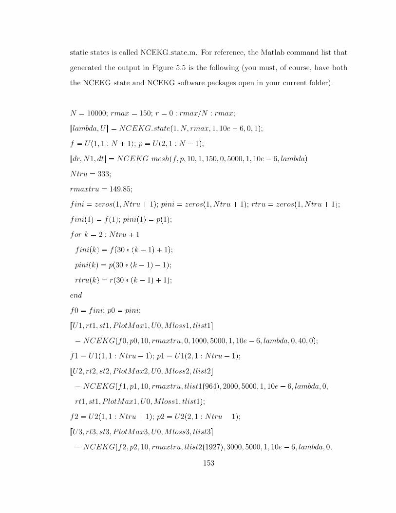
static states is called NCEKG state.m. For reference, the Matlab command list that
generated the output in Figure 5.5 is the following (you must, of course, have both
the NCEKG state and NCEKG software packages open in your current folder).
N 10000; rmax 150; r 0 : rmaxN : rmax;
rlambda, U s NCEKG statep1, N, rmax, 1, 10e 6, 0, 1q;f Up1, 1 : N 1q; p Up2, 1 : N 1q;rdr,N1, dts NCEKG meshpf, p, 10, 1, 150, 0, 5000, 1, 10e 6, lambdaqNtru 333;
rmaxtru 149.85;
fini zerosp1, Ntru 1q; pini zerosp1, Ntru 1q; rtru zerosp1, Ntru 1q;finip1q fp1q; pinip1q pp1q;for k 2 : Ntru 1
finipkq fp30 pk 1q 1q;pinipkq pp30 pk 1q 1q;rtrupkq rp30 pk 1q 1q;
end
f0 fini; p0 pini;
rU1, rt1, st1, P lotMax1, U0,Mloss1, tlist1s NCEKGpf0, p0, 10, rmaxtru, 0, 1000, 5000, 1, 10e 6, lambda, 0, 40, 0q;
f1 U1p1, 1 : Ntru 1q; p1 U1p2, 1 : Ntru 1q;rU2, rt2, st2, P lotMax2, U0,Mloss2, tlist2s NCEKGpf1, p1, 10, rmaxtru, tlist1p964q, 2000, 5000, 1, 10e 6, lambda, 0,
rt1, st1, P lotMax1, U0,Mloss1, tlist1q;f2 U2p1, 1 : Ntru 1q; p2 U2p2, 1 : Ntru 1q;rU3, rt3, st3, P lotMax3, U0,Mloss3, tlist3s NCEKGpf2, p2, 10, rmaxtru, tlist2p1927q, 3000, 5000, 1, 10e 6, lambda, 0,
153

rt2, st2, P lotMax2, U0,Mloss2, tlist2q;f3 U3p1, 1 : Ntru 1q; p3 U3p2, 1 : Ntru 1q;rU4, rt4, st4, P lotMax4, U0,Mloss4, tlist4s NCEKGpf3, p3, 10, rmaxtru, tlist3p2890q, 4000, 5000, 1, 10e 6, lambda, 0,
rt3, st3, P lotMax3, U0,Mloss3, tlist3q;f4 U4p1, 1 : Ntru 1q; p4 U4p2, 1 : Ntru 1q;rU5, rt5, st5, P lotMax5, U0,Mloss5, tlist5s NCEKGpf4, p4, 10, rmaxtru, tlist4p3853q, 5000, 5000, 1, 10e 6, lambda, 0,
rt4, st4, P lotMax4, U0,Mloss4, tlist4q;f5 U5p1, 1 : Ntru 1q; p5 U5p2, 1 : Ntru 1q;
On the other hand, we plot in Figure 5.6 the real version of a first excited state
evolved for a certain amount of time. Since there are no complex components in this
case, as the Einstein-Klein-Gordon equations do not inherently generate complex
values, we will plot simply f , instead of the three functions we plot in the complex
case. Thus there are only six plots plotted in this version. This is how the program
automatically treats all real solutions.
By choosing a vidtype of 1 or 2, the program will generate individual plots of
each of these functions. This is useful if one wished to make a more detailed analysis
of the evolution of just one of these equations.
The program set can be found on Hubert Bray’s wave dark matter web page found
at http://www.math.duke.edu/~bray/darkmatter/darkmatter.html and is called
NCEKG, an acronym for Newtonian Compatible Einstein-Klein-Gordon. All of the
functions are well annotated to explain what each function does and how it does it.
154

Figure 5.5: Output plot generated by the NCEKG program for a complex scalar field. The upper left panel depicts theabsolute value of the scalar field, while the first two panels on the bottom row are plots of the real and imaginary parts ofthe scalar field respectively. The second and third upper panels are plots of the potential and mass functions respectively.The vertical dotted line in the plot of the potential traces the position of a particle in free fall in the system. The lasttwo plots on the bottom row are plots of the energy density function µ and µ times the surface area of a metric sphere ofradius r. The upper right panel plots the difference between the current value of M at r rmax the initial value of Mat r rmax as a function of t. This “mass lost” plot can be a visual measure of the error if the plot in question is notsupposed to lose mass, or it can serve as a visual representation of the mass lost due to escaping waves.
155

Figure 5.6: Output plot generated by the NCEKG program for a real scalar field. The upper left panel plots the scalarfield. The second and third upper panels are plots of the potential and mass functions respectively. The vertical dottedline in the plot of the potential traces the position of a particle in free fall in the system. The first two plots on the bottomrow are plots of the energy density function µ and µ times the surface area of a metric sphere of radius r. The lower rightpanel plots the difference between the current value of M at r rmax the initial value of M at r rmax as a function oft. This “mass lost” plot can be a visual measure of the error if the plot in question is not supposed to lose mass, or it canserve as a visual representation of the mass lost due to escaping waves.
156

6
Conclusions
In this short concluding chapter, we summarize the main results of this dissertation.
In this dissertation, we have considered a possible description of dark matter called
wave dark matter, which uses a scalar field to model the dark matter. Specifically,
we have considered a spherically symmetric spacetime with a scalar field and metric
that satisfies the Einstein-Klein-Gordon equations. We have compared the properties
of such a spacetime with observations of dwarf spheroidal galaxies with the hopes of
constraining the fundamental constant of the Einstein-Klein-Gordon equations, Υ.
To do this, we have surveyed the result that the Einstein equation under a general
spherically symmetric metric of the form in (2.20) is remarkably simple. In particular,
it defines a first order system of partial differential equations. The Klein-Gordon
equation can be used to complete this system to evolve the metric corresponding to
a complex scalar field. Moreover, for a scalar field of the form
fpt, rq eiωtF prq, (6.1)
with ω P R, we have shown that the metric is static if and only if F eiahprq for a
real constant a and a real valued function h. Without loss of generality, we consider
157

these static solutions where a 0. These solutions can be distinguished by the
number, n, of zeros they contain and are called static ground states when n 0 and
static nth excited states otherwise.
We compared these static states to the Burkert dark matter mass profiles com-
puted by Salucci et al. (Salucci et al. (2012)) in order to constrain Υ. We found that
under precise assumptions, a value of
Υ 50 yr1 (6.2)
produces wave dark matter mass models that are qualitatively similar to the Burkert
mass models found by Salucci et al. We also showed that comparisons to these
Burkert profiles can be used to bound the value of Υ by
Υ ¤ 1000 yr1. (6.3)
Our future work will continue in this vein, using the numerical scheme described
in Chapter 5 to numerically evolve the spherically symmetric Einstein-Klein-Gordon
equations. With this tool, we can remove the assumption that the metric is static and
consider more generic solutions of the spherically symmetric Einstein-Klein-Gordon
equations. We plan to directly compare these to observations of dwarf spheroidal
galaxies in the hopes of obtaining a better estimate of the constant Υ. These results
will help us in our ultimate quest of determining if dark matter in the universe can
be described by this wave dark matter theory.
158

Appendix A
The Derivation of theEinstein-Klein-Gordon Equations
In this appendix, we derive the Einstein-Klein-Gordon system of equations for a
complex scalar field by computing the Euler-Lagrange equations of its corresponding
action on the manifold.
Let pN, gq be a (3+1)-dimensional Lorentzian spacetime without boundary, where
g is the metric. Let f : N Ñ C be a complex scalar field on the manifold. Let U N
be any open set for which a coordinate chart is defined. Consider the action on U N
given by
Fpg, fq »U
R 2Λ 16πµ0
|df |2Υ2
|f |2dV (A.1)
with Υ P R. This action arises in a natural way from the axioms of general relativity
as described by Bray (Bray (2010)). We seek a pair pg, fq that is a critical point of
F with respect to any variation of pg, fq that is compactly supported in U for any
U . We compute the critical point via computing the Euler-Lagrange equations.
To compute the Euler-Lagrange equations of this action, we will vary g and f
159

independently and compute the conditions under which pg, fq would be a critical
point of F . We will vary the metric g first.
A.1 Varying the Metric
Let gs be a variation of g, compactly supported in U , with g0 g and 9g h, where
the dot will always denote the variational derivatived
dsat s 0. We want to find
the conditions under which pg, fq is a critical point of F for all variations of g. That
is, we wish to solve the equation
d
dsFpgs, fq
s0
0 (A.2)
for g. To this end, we have that
0 d
dsFpgs, fq
s0
d
ds
»U
R 2Λ 16πµ0
|df |2Υ2
|f |2dV
s0
»U
9R 16πµ0
Υ2
d
dsgspdf, dfq
s0
dV
»U
R 2Λ 16πµ0
|df |2Υ2
|f |2
9dV (A.3)
It is well known that under a variation of the metric, the following are true
9R xh,Ricyg ∇ p∇ hq ∆ptrg hq, (A.4)
9dV 1
2trg h dV, (A.5)
9gµν hµν . (A.6)
160

Now write f fR ifC , where fR Repfq and fC Impfq. Since f is independent
of the variation, then by (A.6), we have that
d
dsgspdf, dfq
s0
d
dsgµνs pfRµ ifCµ qpfRν ifCν q
s0
hµνpfRµ fRν fCµ fCν ifRµ f
Cν ifCµ f
Rν q
hµνpfRµ fRν fCµ fCν q
@h, dfR b dfR dfC b dfCDg
(A.7)
where the subscripts on f denote partial differentiation and the second to last line is
obtained from the previous one by relabeling of the indices on the purely imaginary
terms. Now on the other hand,
1
2pdf b df df b dfq 1
2
dfR idfC
b dfR idfC
dfR idfCb dfR idfC
1
2
2dfR b dfR 2dfC b dfC idfR b dfC
idfC b dfR idfR b dfC idfC b dfR
dfR b dfR dfC b dfC . (A.8)
This makes (A.7) become
d
dsgspdf, dfq
s0
Bh,
1
2
df b df df b df
Fg
. (A.9)
161

Next, equations (A.4), (A.5), and (A.7), and the fact that trg h xg, hyg make (A.3)
become
0 »U
xh,Ricyg ∇ p∇ hq ∆ptrg hq
16πµ0
Υ2
Bh,
1
2
df b df df b df
Fg
dV
»U
R 2Λ 16πµ0
|df |2Υ2
|f |2
1
2xh, gyg
dV
»U
xh,Ricyg 8πµ0
Υ2
@h, df b df df b df
Dg
Ch,
1
2R Λ 8πµ0
|df |2Υ2
|f |2
g
Gg
dV
»U
∇ p∇ hq dV »U
∆ptrg hq dV.
»U
Ch,G Λg 8πµ0
df b df df b df
Υ2|df |2Υ2
|f |2g
Gg
dV
»U
∇ p∇ hq dV »U
∇ ∇ptrg hq dV.
0 »U
Ch,G Λg 8πµ0
df b df df b df
Υ2|df |2Υ2
|f |2g
Gg
dV
»BU∇ h dV
»BU∇ptrg hq dV (A.10)
where G Ric12Rg is the Einstein curvature tensor. The last line uses the diver-
gence theorem. Since the variation gs is compactly supported in U , making h 0
on BU , the last two terms here are zero. Since we want (A.10) to be true for all
compactly supported variations on any coordinate chart, we must require that
G Λg 8πµ0
df b df df b df
Υ2|df |2Υ2
|f |2g
(A.11)
162

on all of N . This equation is the Einstein equation in the presence of a scalar field.
A.2 Varying the Scalar Field
Next, consider a variation of f , fs, compactly supported in U with f0 f and 9f q.
In this case, we want a condition under which pg, fq is a critical point of F for all
variations of f . This time, since g is independent of the variation, we have that
0 d
dsFpg, fsq
s0
d
ds
»U
R 2Λ 16πµ0
|dfs|2Υ2
|fs|2dV
s0
»U
16πµ0d
ds
|dfs|2Υ2
|fs|2
s0
dV (A.12)
Now,
d
ds|fs|2
s0
d
dsfsfs
s0
qf f q (A.13)
and
d
dsgdfs, dfs
s0
d
dsg∇fs,∇fs
s0
g p∇f,∇qq g p∇q,∇qq . (A.14)
Then (A.12) becomes
0 16πµ0
»U
1
Υ2
g p∇f,∇qq g
∇q,∇f
qf f q dV. (A.15)
By the divergence theorem and the fact that the variation is compactly supported
in U so that q 0 on BU ,
0 »U
∇ pq∇fq dV »U
g p∇q,∇fq q2gf dV (A.16)
0 »U
∇ q∇f dV »U
g∇q,∇f
q2gf dV (A.17)
163

Equations (A.15) - (A.17) imply that
0 16πµ0
»U
1
Υ2
q2gf q2gf qf qf dV
16πµ0
Υ2
»U
qΥ2f 2gf
qΥ2f 2gf
dV. (A.18)
Equation (A.18) holds for all compactly supported variations of f in any coordinate
chart. This implies that
2gf Υ2f (A.19)
on all of N . This equation is called the Klein-Gordon equation.
A.3 The Einstein-Klein-Gordon Equations
We have shown that the Euler-Lagrange equations for the action (A.1) are (A.11)
and (A.19), which are rewritten below for convenience.
G Λg 8πµ0
df b df df b df
Υ2|df |2Υ2
|f |2g
(A.20a)
2gf Υ2f. (A.20b)
These paired equations are called the Einstein-Klein-Gordon equations.
164

Bibliography
Alcubierre, M. (2008), Introduction to 3 1 Numerical Relativity, Oxford UniversityPress, Oxford.
Alcubierre, M., Allen, G., Brugmann, B., Seidel, E., and Suen, W.-M. (2000), “To-wards an Understanding of the Stability Properties of the 31 Evolution Equationsin General Relativity,” Phys. Rev. D, 62, 124011.
Alic, D., Bona, C., Bona-Casas, C., and Masso, J. (2007), “Efficient Implementationof Finite Volume Methods in Numerical Relativity,” Physical Review D, 76, 10.
Arnowitt, R., Deser, S., and Misner, C. (2008), “Republication of: The Dynam-ics of General Relativity,” General Relativity and Gravitation, 40, 1997–2027,10.1007/s10714-008-0661-1.
Balakrishna, J., Seidel, E., and Suen, W.-M. (1998), “Dynamical Evolution of BosonStars. II. Excited States and Self-interacting Fields,” Phys. Rev. D, 58, 104004.
Baumgarte, T. W. and Shapiro, S. L. (2010), Numerical Relativity: Solving Einstein’sEquations on the Computer, Cambridge University Press.
Begeman, K. G. (1989), “HI Rotation Curves of Spiral Galaxies,” Astronomy andAstrophysics, 223, 47–60.
Bender, C. M. and Orszag, S. A. (1978), Advanced Mathematical Methods for Scien-tists and Engineers: Asymptotic Methods and Perturbation Theory, McGraw-Hill,New York.
Bernal, A., Matos, T., and Nunez, D. (2008), “Flat Central Density Profiles fromScalar Field Dark Matter Halos,” Revista Mexicana de Astronomıa y Astrofısica,44, 149–160.
Bernal, A., Barranco, J., Alic, D., and Palenzuela, C. (2010), “Multistate BosonStars,” Phys. Rev. D, 81, 044031.
Bertone, G., Hooper, D., and Silk, J. (2005), “Particle Dark Matter: Evidence,Candidates and Constraints,” Physics Reports, 405, 279–390.
165

Billouin, L. (1926), “La mecanique ondulatoire de Schrodinger; une methode generalede resolution par approximations successives,” Comptes Rendus de l’Academie desSciences, 183, 24–26.
Binney, J. and Merrifield, M. (1998), Galactic Astronomy, Princeton Series in As-trophysics, Princeton University Press.
Binney, J. and Tremaine, S. (2008), Galactic Dynamics, Princeton Series in Astro-physics, Princeton University Press.
Birkhoff, G. D. (1923), Relativity and Modern Physics, Harvard University Press.
Bona, C. and Masso, J. (1992), “Hyperbolic Evolution System for Numerical Rela-tivity,” Phys. Rev. Lett., 68, 1097–1099.
Bona, C., Ledvinka, T., and Palenzuela, C. (2002), “3+1 Covariant Suite of Numer-ical Relativity Evolution Systems,” Phys. Rev. D, 66, 084013.
Bosma, A. (1981), “21-cm Line Studies of Spiral Galaxies. I - Observations of theGalaxies NGC 5033, 3198, 5055, 2841, and 7331. II - The Distribution and Kine-matics of Neutral Hydrogen in Spiral Galaxies of Various Morphological Types,”The Astrophysical Journal, 86, 1791–1846.
Bray, H. (2001), “Proof of the Riemannian Penrose Inequality Using the PositiveMass Theorem,” Journal of Differential Geometry, 59, 177–267.
Bray, H. (2010), “On Dark Matter, Spiral Galaxies, and the Axioms of GeneralRelativity,” accepted, to appear in an AMS Contemporary Mathematics Volumein 2013.
Bray, H. (2012), “On Dark Matter, Shells in Elliptical Galaxies, and the Axioms ofGeneral Relativity,” [arXiv:1212.5745 [physics.gen-ph]].
Bray, H., Hayward, S., Mars, M., and Simon, W. (2007), “Generalized Inverse MeanCurvature Flows in Spacetime,” Commun. Math. Phys., 272, 119–138.
Bray, H. L. and Parry, A. R. (2013), “Modeling Wave Dark Matter in Dwarf Spher-oidal Galaxies,” [arXiv:1301.0255 [astro-ph.GA]].
Burkert, A. (1995), “The Structure of Dark Matter Halos in Dwarf Galaxies,” TheAstrophysical Journal Letters, 447, L25.
Carlini, F. (1817), Ricerche sulla convergenza della serie che serva alla soluzione delproblema di Keplero, Milan.
Choptuik, M. W. (1998), “UT Austin PHY387N Lec-ture Notes,” Retrieved online on Nov. 1, 2011 atlaplace.phas.ubc.ca/People/matt/Teaching/98Spring/Phy387N/Syllabus.html.
166

Conroy, C., Loeb, A., and Spergel, D. (2011), “Evidence Against Dark Matter HalosSurrounding the Globular Clusters MGC1 and NGC 2419,” .
Cordero-Carrion, I., Ibenez, J. M., and Morales-Lladosa, J. A. (2011), “MaximalSlicings in Spherical Symmetry: Local Existence and Construction,” J. Math.Phys., 52.
Cote, P., Mateo, M., Olszewski, E. W., and Cook, K. H. (1999), “Internal Kinematicsof the Andromeda II Dwarf Spheroidal Galaxy,” The Astrophysical Journal, 526,147.
Dahle, H. (2007), “A Compilation of Weak Gravitational Lensing Studies of Clustersof Galaxies,” [arXiv:astro-ph/0701598].
de Blok, W. J. G. (2010), “The Core-Cusp Problem,” Advances in Astronomy, 2010.
den Bergh, V. (2008), “Globular Clusters and Dwarf Spheroidal Galaxies,” MonthlyNotices of the Royal Astronomical Society: Letters, 385, L20–L22.
Deser, S. and Ryzhov, A. V. (2005), “Curvature Invariants of Static SphericallySymmetric Geometries,” Classical and Quantum Gravity, 22, 3315.
Einstein, A. (1905), “Zur Elektrodynamik bewegter Korper,” Annalen der Physik,17, 891.
Einstein, A. (1916), “Die Grundlage der allgemeinen Relativitatstheorie,” Annalender Physik, 354, 769–822.
Eric Gourgoulhon (2012), 31 Formalism in General Relativity: Bases of NumericalRelativity, Springer, Berlin.
Gentile, G., Salucci, P., Klein, U., Vergani, D., and Kalberla, P. (2004), “The CoredDistribution of Dark Matter in Spiral Galaxies,” Monthly Notices of the RoyalAstronomical Society, 351, 903–922.
Gleiser, M. and Watkins, R. (1989), “Gravitational Stability of Scalar Matter,” Nu-clear Physics B, 319, 733–746.
Gottlieb, S., Shu, C.-W., and Tadmor, E. (2001), “Strong Stability-Preserving High-Order Time Discretization Methods,” SIAM Rev, 43, 89–112.
Green, E. G. (1838), “On the Motion of Waves in a variable Canal of small Depthand Width,” Transactions of the Cambridge Philosophical Society, 6, 457.
Guzman, F. S. and Matos, T. (2000), “Scalar fields as dark matter in spiral galaxies,”Classical and Quantum Gravity, 17, L9.
167

Guzman, F. S., Matos, T., and Villegas-Brena, H. (2001), “Scalar Dark Matter inSpiral Galaxies,” Rev. Mex. Astron. Astrofis., 37, 63–72.
Hawking, S. (1968), “Gravitational Radiation in an Expanding Universe,” J. Math.Phys., 9, 598–604.
Hawley, S. H. and Choptuik, M. W. (2000), “Boson Stars Driven to the Brink ofBlack Hole Formation,” Phys. Rev. D, 62, 104024.
Hawley, S. H. and Choptuik, M. W. (2003), “Numerical Evidence for “MultiscalarStars”,” Phys. Rev. D, 67, 024010.
Hilbert, D. (1915), “Die Grundlagen der Physik (Erste Mitteilung),” Nachrichten vonder Gesellschaft der Wissenschaften zu Gottingen, Mathematisch-physikalischeKlasse, 395–407.
Hinshaw, G., Weiland, J. L., Hill, R. S., Odegard, N., Larson, D., Bennett, C. L.,Dunkley, J., Gold, B., Greason, M. R., Jarosik, N., Komatsu, E., Nolta, M. R.,Page, L., Spergel, D. N., Wollack, E., Halpern, M., Kogut, A., Limon, M., Meyer,S. S., Tucker, G. S., and Wright, E. L. (2009), “Five-Year Wilkinson MicrowaveAnisotropy Probe Observations: Data Processing, Sky Maps, and Basic Results,”The Astrophysical Journal Supplement Series, 180, 225.
Hooper, D. and Baltz, E. A. (2008), “Strategies for Determining the Nature of DarkMatter,” Ann.Rev.Nucl.Part.Sci., 58, 293–314.
Huisken, G. and Ilmanen, T. (2001), “The Inverse Mean Curvature Flow and theRiemannian Penrose Inequality,” Journal of Differential Geometry, 59, 353–437.
Humphrey, P. J., Buote, D. A., Gastaldello, F., Zappacosta, L., Bullock, J. S.,Brighenti, F., and Mathews, W. G. (2006), “A Chandra View of Dark Matter inEarly-Type Galaxies,” The Astrophysical Journal, 646, 899.
Jebson, J. T. (1921), “Uber die allgemeinen kugelsymmetrischen Loosungen der Ein-steinschen Gravitationsgleichungen im Vakuum,” Arkiv for Matematik, Astronomioch Fysik, 15.
Ji, S. U. and Sin, S. J. (1994), “Late-Time Phase Transition and the Galactic Haloas a Bose Liquid. II. The Effect of Visible Matter,” Phys. Rev. D, 50, 3655–3659.
King, I. (1962), “The structure of star clusters. I. an empirical density law,” TheAstronomical Journal, 67, 471.
Kleyna, J., Wilkinson, M. I., Evans, N. W., Gilmore, G., and Frayn, C. (2002), “DarkMatter in Dwarf Spheroidals - II. Observations and Modelling of Draco,” MonthlyNotices of the Royal Astronomical Society, 330, 792–806.
168

Kramers, H. A. (1926), “Wellenmechanik und halbzahlige Quantisierung,” Zeitschriftfur Physik, 39, 828–840.
Kreiss, H. and Oliger, J. (1973), “Methods for the Approximate Solution of Time De-pendent Problems,” Global Atmospheric Research Programme Publication Series,10.
Lai, C. W. (2004), “A Numerical Study of Boson Stars,” Ph.D. thesis, The Universityof British Columbia.
Lai, C. W. and Choptuik, M. W. (2007), “Final Fate of Subcritical Evolutions ofBoson Stars,” [arXiv:0709.0324 [gr-qc]].
Lee, J.-W. (2009), “Is Dark Matter a BEC or Scalar Field?” Journal of the KoreanPhysical Society, 54, 2622.
Lee, J.-W. and Koh, I.-G. (1992), “Galactic Halo as a Soliton Star,” Abstracts,Bulletin of the Korean Physical Society, 10.
Lee, J.-W. and Koh, I.-G. (1996), “Galactic Halos as Boson Stars,” Phys. Rev. D,53, 2236–2239.
Liouville, J. (1837), “Sur le developpement des fonctions et series..” Journal deMathematiques Pures et Appliquees, 1.
Mashchenko, S., Sills, A., and Couchman, H. M. (2006), “Constraining Global Prop-erties of the Draco Dwarf Spheroidal Galaxy,” The Astrophysical Journal, 640,252.
Mateo, M. (1998), “Dwarf Galaxies of the Local Group,” Annual Review of Astron-omy and Astrophysics, 36, 435–506.
Matos, T. and na Lopez, L. A. U. (2000), “Quintessence and Scalar Dark Matter inthe Universe,” Classical and Quantum Gravity, 17, L75.
Matos, T. and Urena Lopez, L. A. (2001), “Further Analysis of a Cosmological Modelwith Quintessence and Scalar Dark Matter,” Phys. Rev. D, 63, 063506.
Matos, T., Vazquez-Gonzalez, A., and Magana, J. (2009), “ϕ2 as dark matter,”Monthly Notices of the Royal Astronomical Society, 393, 1359–1369.
Minkowski, H. (1908), “Raum und Zeit,” Physikalishe Zeitschrift, 10, 75–88.
Navarro, J. F., Frenk, C. S., and White, S. D. M. (1996), “The Structure of ColdDark Matter Halos,” The Astrophysical Journal, 462, 563.
O’Neill, B. (1983), Semi-Riemannian Geometry with Applications to Relativity, Aca-demic Press, San Diego.
169

Oort, J. H. (1932), “The Force Exerted by the Stellar System in the Direction Per-pendicular to the Galactic Plane and Some Related Problems,” Bulletin of theAstronomical Institutes of the Netherlands, 6, 249.
Ostriker, J. (1993), “Astronomical Tests of the Cold Dark Matter Scenario,” AnnualReview of Astronomy and Astrophysics, 31, 689–716.
Parry, A. R. (2007), “A Classification of Real Indecomposable Solvable Lie Algebrasof Small Dimension with Codimension One Nilradicals,” Master’s thesis, UtahState University.
Parry, A. R. (2012a), “Spherically Symmetric Static States of Wave Dark Matter,”[arXiv:1212.6426 [gr-qc]].
Parry, A. R. (2012b), “A Survey of Spherically Symmetric Spacetimes,”[arXiv:1210.5269 [gr-qc]].
Perlmutter, S., Aldering, G., Goldhaber, G., Knop, R. A., Nugent, P., Castro, P. G.,Deustua, S., Fabbro, S., Goobar, A., Groom, D. E., Hook, I. M., Kim, A. G.,Kim, M. Y., Lee, J. C., Nunes, N. J., Pain, R., Pennypacker, C. R., Quimby, R.,Lidman, C., Ellis, R. S., Irwin, M., McMahon, R. G., Ruiz-Lapuente, P., Walton,N., Schaefer, B., Boyle, B. J., Filippenko, A. V., Matheson, T., Fruchter, A. S.,Panagia, N., Newberg, H. J. M., Couch, W. J., and Project, T. S. C. (1999),“Measurements of Omega and Lambda from 42 High-Redshift Supernovae,” TheAstrophysical Journal, 517, 565.
Primack, J. R., Seckel, D., and Sadoulet, B. (1988), “Detection of Cosmic DarkMatter,” Ann.Rev.Nucl.Part.Sci., 38, 751–807.
Riess, A. G., Filippenko, A. V., Challis, P., Clocchiatti, A., Diercks, A., Garnavich,P. M., Gilliland, R. L., Hogan, C. J., Jha, S., Kirshner, R. P., Leibundgut, B.,Phillips, M. M., Reiss, D., Schmidt, B. P., Schommer, R. A., Smith, R. C., Spy-romilio, J., Stubbs, C., Suntzeff, N. B., and Tonry, J. (1998), “ObservationalEvidence from Supernovae for an Accelerating Universe and a Cosmological Con-stant,” The Astronomical Journal, 116, 1009–1038.
Salucci, P., Martins, C. F., and Lapi, A. (2010), “DMAW 2010 LEGACY the Pre-sentation Review: Dark Matter in Galaxies with its Explanatory Notes,” .
Salucci, P., Wilkinson, M. I., Walker, M. G., Gilmore, G. F., Grebel, E. K., Koch,A., Frigerio Martins, C., and Wyse, R. F. G. (2012), “Dwarf Spheroidal GalaxyKinematics and Spiral Galaxy Scaling Laws,” Monthly Notices of the Royal Astro-nomical Society, 420, 2034–2041.
Schoen, R. and Yau, S.-T. (1979), “On the Positive Mass Conjecture in GeneralRelativity,” Commun. Math. Phys., 65, 45–76.
170

Schoen, R. and Yau, S.-T. (1981), “Proof of the Positive Mass Theorem. II,” Com-mun. Math. Phys., 79, 231–260.
Schunck, F. and Mielke, E. (2003), “General relativistic boson stars,” Classical andQuantum Gravity, 20, R301–R356.
Seidel, E. and Suen, W.-M. (1990), “Dynamical Evolution of Boson Stars: Perturbingthe Ground State,” Phys. Rev. D, 42, 384–403.
Sharma, R., Karmakar, S., and Mukherjee, S. (2008), “Boson Star and Dark Matter,”[arXiv:0812.3470 [gr-qc]].
Sin, S.-J. (1994), “Late-Time Phase Transition and the Galactic Halo as a BoseLiquid,” Phys. Rev. D, 50, 3650–3654.
Strigari, L. E., Koushiappas, S. M., Bullock, J. S., Kaplinghat, M., Simon, J. D.,Geha, M., and Willman, B. (2008), “The Most Dark-Matter-dominated Galax-ies: Predicted Gamma-Ray Signals from the Faintest Milky Way Dwarfs,” TheAstrophysical Journal, 678, 614.
Trimble, V. (1987), “Existence and Nature of Dark Matter in the Universe,” AnnualReview of Astronomy and Astrophysics, 25, 425–472.
Wald, R. M. (1984), General Relativity, The Univeristy of Chicago Press, Chicago.
Walker, M. G., Mateo, M., Olszewski, E. W., Gnedin, O. Y., Wang, X., Sen, B., andWoodroofe, M. (2007), “Velocity Dispersion Profiles of Seven Dwarf SpheroidalGalaxies,” The Astrophysical Journal Letters, 667, L53.
Walker, M. G., Mateo, M., Olszewski, E. W., narrubia, J. P., Evans, N. W., andGilmore, G. (2009), “A Universal Mass Profile for Dwarf Spheroidal Galaxies?”The Astrophysical Journal, 704, 1274.
Walker, M. G., Mateo, M., Olszewski, E. W., narrubia, J. P., Evans, N. W., andGilmore, G. (2010), “Erratum: “A Universal Mass Profile for Dwarf SpheroidalGalaxies?” (2009, ApJ, 704, 1274),” The Astrophysical Journal, 710, 886.
Wentzel, G. (1926), “Eine Verallgemeinerung der Quantenbedingungen fur dieZwecke der Wellenmechanik,” Zeitschrift fur Physik, 38, 518–529.
Zwicky, F. (1933), “Die Rotverschiebung von extragalaktischen Nebeln,” HelveticaPhysica Acta, 6, 110–127.
171
Biography
Alan Reid Parry was born in Ogden, UT on April 21, 1983. He graduated Magna
Cum Laude with a Bachelor of Science degree in Mathematics from Utah State Uni-
versity on May 6, 2006. He also received a Master of Science degree in Mathematics
from Utah State University on December 15, 2007, for which he worked with Ian An-
derson and wrote a thesis entitled “A Classification of Real Indecomposable Solvable
Lie Algebras of Small Dimension with Codimension One Nilradicals” (Parry (2007)).
Alan earned a Master of Arts degree in Mathematics from Duke University on
December 30, 2008. He worked with Hubert Bray on research that culminated in
this dissertation, which he defended on March 1, 2013. Duke University conferred
on him the degree of Doctor of Philosophy in Mathematics on May 12, 2013.
While a graduate student, Alan was the sole author of two papers and a joint
author of a paper with Hubert Bray. These are entitled “A Survey of Spherically
Symmetric Spacetimes” (Parry (2012b)), “Spherically Symmetric Static States of
Wave Dark Matter” (Parry (2012a)), and “Modeling Wave Dark Matter in Dwarf
Spheroidal Galaxies” (Bray and Parry (2013)). The majority of this dissertation
consists of the work presented in these three papers.
He also received the L.P. and Barbara Smith Award for Beginning Teachers in
February 2009 and the L.P. and Barbara Smith Award for Teaching Excellence in
September 2010 from the Mathematics department at Duke University. Alan will
continue his career as a Visiting Assistant Professor at the University of Connecticut.
172