water supply system management design...
TRANSCRIPT

Water Supply System Management Designand Optimization under Uncertainty
Item Type text; Electronic Dissertation
Authors Chung, Gunhui
Publisher The University of Arizona.
Rights Copyright © is held by the author. Digital access to this materialis made possible by the University Libraries, University of Arizona.Further transmission, reproduction or presentation (such aspublic display or performance) of protected items is prohibitedexcept with permission of the author.
Download date 26/05/2018 23:47:08
Link to Item http://hdl.handle.net/10150/195506
WATER SUPPLY SYSTEM MANAGEMENT DESIGN AND OPTIMIZATION
UNDER UNCERTAINTY
by
GUNHUI CHUNG
_______________________ Copyright © Gunhui Chung 2007
A Dissertation Submitted to the Faculty of the
DEPARTMENT OF CIVIL ENGINEERING AND ENGINEERING MECHANICS
In Partial Fulfillment of the Requirements
For the Degree of
DOCTOR OF PHILOSOPHY WITH A MAJOR IN CIVIL ENGINEERING
In the Graduate College
THE UNIVERSITY OF ARIZONA
2007

2
THE UNIVERSITY OF ARIZONA GRADUATE COLLEGE
As members of the Dissertation Committee, we certify that we have read the dissertation
prepared by GUNHUI CHUNG
entitled WATER SUPPLY SYSTEM MANAGEMENT DESIGN AND
OPTIMIZATION UNDER UNCERTAINTY
and recommend that it be accepted as fulfilling the dissertation requirement for the
Degree of DOCTOR OF PHILOSOPHY
_______________________________________________________________________ Dr. Kevin Lansey Date: December 4, 2006 _______________________________________________________________________ Dr. Juan Valdes Date: December 4, 2006 _______________________________________________________________________ Dr. Larry W. Mays Date: December 4, 2006 _______________________________________________________________________ Dr. Donald R. Davis Date: December 4, 2006 _______________________________________________________________________ Dr. Guzin Bayraksan Date: December 4, 2006 _______________________________________________________________________ Dr. Bart Nijssen Date: December 4, 2006 Final approval and acceptance of this dissertation is contingent upon the candidate’s submission of the final copies of the dissertation to the Graduate College. I hereby certify that I have read this dissertation prepared under my direction and recommend that it be accepted as fulfilling the dissertation requirement. ________________________________________________ Date: December 4, 2006 Dissertation Director: Dr. Kevin Lansey

3
STATEMENT BY AUTHOR
This dissertation has been submitted in partial fulfillment of requirements for an advanced
degree at The University of Arizona and is deposited in the University Library to be made
available to borrowers under rules of the Library.
Brief quotations from this dissertation are allowable without special permission, provided
that accurate acknowledgment of source is made. Requests for permission for extended
quotation from or reproduction of this manuscript in whole or in part may be granted by the
copyright holder.
SIGNED: Gunhui Chung

4
ACKNOWLEDGEMENTS
I would like to express my gratitude to all those who help me to complete this dissertation.
I am deeply indebted to my advisor Dr. Lansey for all his support during this work. He was
the one who gave me the opportunity and his restless guides, suggestions and encouragement
made it possible for me to complete this dissertation.
I would like to thank Dr. Bayraksan for her invaluable advices to overcome whenever
seemingly unsolvable problems challenged me. Without her help, this study could not have
been completed.
I also want to thank my other committee, Dr. Valdes, Dr. Mays, Dr. Davis, and Dr. Nijssen
for their generosity and invaluable comments to my humble works. It was my honor to have
such respectful scholars as my committee members.
My special thank goes to Chinmaya for helping me out in C ++ coding. I am also grateful to
all friends of mine, including Jim, Amanda, Richard, Pasha, David, Doo Sun and Tae-
Woong, for their help and friendship. All of you listened to me sincerely, always took my
side and helped me to get over it when I was in trouble.
Especially, I would like to thank Derya, my best friend. She made my closed mind open with
her sincere friendship and helped me survive in unfamiliar environment. I am sure that she
will become a great scholar.
I also want to thank my family, father, mother and two brothers, Chul-Ho and Min-Suk, for
their endless support. Chul-Ho helped me a lot when I started working on computer
programming. Their warm heart is always with me wherever I go.
Finally, I would like to give my special thanks to my husband Inhong whose patient love
gave me strength to confront whatever I was up to.
5
TABLE OF CONTENTS ABSTRACT ........................................................................................................................ 9
1. INTRODUCTION ........................................................................................................ 11
1.1 Problem Statement .................................................................................................. 11
1.2 Literature Review.................................................................................................... 12
1.2.1 Water Supply System Design .......................................................................... 12
1.2.2 Deterministic Optimization .............................................................................. 15
1.2.3 Stochastic Optimization ................................................................................... 16
1.3 Summary of Literature ............................................................................................ 18
2. PRESENT STUDY ....................................................................................................... 19
2.1 Dissertation Outline ................................................................................................ 19
2.2 Uniqueness of the Study ......................................................................................... 34
2.3 Conclusions and Future Work ................................................................................ 36
REFERENCES ................................................................................................................. 39
APPENDIX A: A GENERAL WATER RESOURECES PLANNING MODEL USING
DYNAMIC SIMULATION: EVALUATION OF DECENTRALIZED TREATMENT 46
ABSTRACT ...................................................................................................................... 47
1. INTRODUCTION ....................................................................................................... 49
2. LITERATURE REVIEW/BACKGROUND ................................................................ 50
3. MODELING TOOLS ................................................................................................... 53
3.1 Modeling Objective ................................................................................................ 53
3.2 Generic System ....................................................................................................... 54
6
3.3 General Components ............................................................................................... 57
3.4 Demand/ User Components .................................................................................... 58
3.5 Water Quality Transformations .............................................................................. 62
4. APPLICATIONS .......................................................................................................... 66
4.1 Scenario 1 – Effectiveness of Conservation Practices ............................................ 69
4.2 Scenario 2 – Unavailability of Supply Sources ...................................................... 72
4.3 Scenario 3 – Decentralized Treatment .................................................................... 73
5. CONCLUSIONS........................................................................................................... 77
6. REFERENCES ............................................................................................................. 80
7. TABLES ....................................................................................................................... 86
8. FIGURES .................................................................................................................... 108
APPENDIX B. APPLICATION OF THE SHUFFLED FROG LEAPING ALGORITHM
FOR THE OPTIMIZATION OF A GENERAL LARGE-SCALE WATER SUPPLY
SYSTEM ......................................................................................................................... 126
ABSTRACT .................................................................................................................... 127
1. INTRODUCTION AND BACKGROUND ............................................................... 129
2. PROBLEM DESCRIPTION ....................................................................................... 131
3. PROBLEM FORMULATION.................................................................................... 132
3.1 Simple Bound Constraints on System Flows and Component Sizes .................... 136
3.2 Node Constraints ................................................................................................... 138
3.3 Arc Related Flow Constraints ............................................................................... 139
3.4 Water Quality Constraints ..................................................................................... 141
7
3.5 Objective Function Penalty Term ......................................................................... 143
3.6 Summary of Formulation ...................................................................................... 144
4. SHUFFLED FROG LEAPING ALGORITHM (SFLA) ............................................ 144
4.1 Global Exploration ................................................................................................ 146
4.2 Local Exploration: Frog Leaping Algorithm (FLA) ............................................. 147
5. APPLICATIONS ........................................................................................................ 151
5.1 Single Wastewater Treatment Plant System ......................................................... 151
5.2 Multiple Wastewater Treatment Plant System ..................................................... 154
6. CONCLUSIONS......................................................................................................... 157
7. NOMENCLATURE ................................................................................................... 159
8. REFERENCES ........................................................................................................... 164
9. TABLES ..................................................................................................................... 166
10. FIGURES .................................................................................................................. 180
APPENDIX C: RELIABLE WATER SUPPLY SYSTEM DESIGN UNDER
UNCERTAINTY ............................................................................................................ 187
ABSTRACT .................................................................................................................... 188
1. INTRODUCTION ...................................................................................................... 190
2. ROBUST OPTIMIZATION FRAMEWORK ............................................................ 192
3. APPLICATION TO WATER SUPPLY SYSTEM .................................................... 199
3.1 Problem Statement ................................................................................................ 199
3.2 Objective Function ................................................................................................ 202
3.3 Simple Decision Bounds ....................................................................................... 204
8
3.4 Flow Constraints through Nodes .......................................................................... 205
3.5 Flow Constraints through Arcs ............................................................................. 207
3.6 Data Uncertainty and Robust Formulation ........................................................... 209
3.7 Probability Bounds................................................................................................ 215
4. RESULTS AND DISCUSSION ................................................................................. 216
5. CONCLUSIONS......................................................................................................... 220
6. NOMENCLATURE ................................................................................................... 223
7. REFERENCES ........................................................................................................... 226
8. TABLES ..................................................................................................................... 229
9. FIGURES .................................................................................................................... 236
9
ABSTRACT
A water supply system collects, treats, stores, and distributes water among water
sources and consumers. Increasing population, diminishing supplies and variable climatic
conditions can cause difficulties in meeting water demands; especially in arid and semi-
arid regions where water resources are limited. Given the system complexity and the
interactions among users and supplies, a large-scale water supply management model can
be useful for decision makers to plan water management strategies to cope with future
water demand changes. When this long range water supply plan is developed, accuracy
and reliability are the two most important factors. To develop an accurate model, as much
information as possible on the system has to be considered. As a result, the water supply
system has become more complicated and comprehensive structures. Stochastic search
techniques thus have evolved to find the most accurate solution for the future water
supply plan. Future uncertainty also has been considered to improve system reliability as
well as economic feasibility. This suite of tools can be also useful in deriving consensus
among competing water needs for proposed long-term water supply plans.
In this study, a general large-scale water supply system that is comprised of modular
components including water sources, users, recharge facilities, and water and wastewater
treatment plants was developed in a dynamic simulation environment that helps users
easily understand the model structure. The model was applied to a realistic hypothetical
system and simulated several possible 20-year planning scenarios. In addition to water
balances and water quality analyses, construction and operation and maintenance of
system components costs were estimated for each scenario. One set of results
10
demonstrates that construction of small-cluster decentralized wastewater treatment
systems could be more economical than a centralized plant when communities are
spatially scattered or located in steep areas where pumping costs may be prohibitive.
The Shuffled Frog Leaping Algorithm (SFLA), then, was used to minimize the total
system cost of the general water supply system. Sizing decisions of system components’
capacities – pipe diameter, pump design capacity and head, canal capacity, and water and
wastewater treatment capabilities – are decision variables with flow allocations over the
water supply network to meet water demands. An explicit representation of energy
consumption cost for the operation of satellite wastewater treatment facilities was
incorporated into the system in the optimization process of overall system cost. Although
the study water supply systems included highly nonlinear terms in the objective function
and constraints and several hundred decisions variables, a stochastic search algorithm
was applied successfully to find optimal solutions that satisfied all the constraints for the
study networks.
An accurate water supply plan is achieved. However, the system reliability is not
assured. A robust optimization approach, hence, was introduced into the design process
of a water supply system as a framework to consider uncertainties of the correlated future
data by applying a new robust optimization approach. The approach allows for the
control of the degree of conservatism which is a crucial factor for the system reliabilities
and economical feasibilities. The system stability is guaranteed under the most uncertain
condition. It was found that the water supply system with uncertainty can be a useful tool
to assist decision makers to develop future water supply schemes.
11
1. INTRODUCTION
1.1 Problem Statement
Providing sufficient water of appropriate quality and quantity has been one of the
most important issues in human history. Most ancient civilizations were initiated near
water sources. As populations grew, the challenge to meet user demands also increased.
People began to transport water from other locations to their communities. For example,
the Romans constructed aqueducts to deliver water from distant sources to their
communities.
Today, a water supply system consists of infrastructure that collects, treats, stores,
and distributes water between water sources and consumers. Limited new natural water
sources, especially in the southwest region of the USA, and rapidly increasing population
has led to the need for innovative methods to manage a water supply system. For
example, reclaimed water has become an essential water resource for potable and non-
potable uses. Structural system additions including new conveyance systems and
treatment and recharge facilities and operation decisions, such as allocating flow and
implementing conservation practices, are made with the present and future demands in
minds. As additional components and linkages between sources and users are developed,
the complexity of the water supply system and the difficulty in understanding how the
system will react to changes grows. The inherent uncertainty in climate and water
demands and supplies further raises the difficulty in interpreting the system. These
concerns raise the need for generalized design tools for decision makers and the public to
12
plan structural changes and manage the water supply system to adapt to future water
demands and supplies. Such tools can be simulation or optimization models and may
directly or indirectly account for system uncertainties.
1.2 Literature Review
Many efforts on the development of a water supply system have been made through
for sustainable water supply. However, the complexity of system limited the site specific
application at the first era. As water demands pressures raise increasingly on the existing
water supply system, many studies attempted to develop a general water supply system to
assist decision makers to design more reliable systems for a long range operation period.
These attempts also include the optimization of total system construction and operation
cost. Under given situations such as limited computational technology, complicatedness
and uncertainty in water supply systems, the ultimate goal of these studies are to supply
water sources to users reliably in a more sustainable and timely manner as a long-term
plan.
1.2.1 Water Supply System Design
Computer-based models together with their interactive interfaces are typically called
as decision support systems (DSS) (Loucks 1995). Despite the limitation of software and
hardware of technology in 1970s and 1980s, many site-specific river basin models were
developed and used by engineers in water management organizations for an operational
planning of their basins (Zagona et al. 2001) such as the U.S. Bureau of Reclamation’s
13
(USBR), Colorado River Simulation System (CRSS), Tennessee Valley Authority’s
(TVA) Daily Scheduling Model, and the Potomac River Interactive Simulation Model
(PRISM). CRSS representative of reservoir system models has been used to establish
complicated operating policies to balance end-of-water-year storage in Lakes Powell and
Mead (USBR, 1987). PRISM was originally developed and implemented to a regional
water supply system for the Washington metropolitan area (Palmer et al. 1980).
To overcome the deficiencies of hard-wired models, several well-supported, general
river and reservoir models such as HEC-5 (Zagona et al. 2001) and HEC-3 (Wurbs 1993)
have been developed to apply policy options that modelers can parameterize and/or
prioritize to represent the operations for a specific system. HEC ResSim (US Army 2003)
and its predecessor, HEC-5, are the two of the most widely used and well documented
reservoir-system simulation models for the operation simulation of a reservoirs system in
a river network for flood control, water supply, hydropower, and instream flow
maintenance for water quality (Wurbs 1993 and Mays and Tung 1992). The HEC-3
Reservoir System Analysis for Conservation program is much simpler than HEC-5 and
does not have the component for the comprehensive flood-control (Wurbs 1993).
Generalized mathematical water management models were also developed by many
researchers. Ocanas and Mays (1981a), Huang and Loucks (2000), and Yang et al. (2000)
applied their reservoir/river management model to hypothetical river networks and
evaluated total cost and benefit of the network. Other applications have a specific
application network such as South Taiwan (Yen and Chen 2001), the Aral Sea basin of
central Asia (Cai et al. 2003), the Rio Grande river from Elephant Butte, New Mexico to
14
Fort Quitman, Texas (Ejeta et al. 2004), Syr Darya River basin (Cai et al. 2001), and
water supply system in southern Israel (Cohen et al. 2004). However, these models could
not be generalized because they did not consider all possible components and thus the
generality and flexibility were not sufficient to allow end-users to easily modify the
model. RiverWare (Biddle 2001, Magee and Goranflo 2002, Gilmore et al. 2000, Fulp
and Harkins 2001) is a general object-oriented model but limited only to reservoir
management.
All previous works mentioned above generally did not incorporate water quality
parameters into the models. Exceptions are the studies conducted by Ocanas and Mays
(1981a and 1981b) that considered biochemical oxygen demand (BOD) and total
suspended solid (TSS) as the water quality parameters. Cai et al. (2001 and 2003) and
Cohen et al. (2004) modeled salinity and Ejeta et al. (2004) incorporated a total dissolved
solid (TDS) component.
Recently, more generalized and object-oriented system dynamics simulation models
have been developed. As one of the earliest applications, Palmer et al. (1993) tailored a
dynamic simulation software application to represent the Portland water supply system.
Other applications include river basin planning (Palmer et al. 2000), long-term water
resource planning and policy analysis (Simonovic et al. 1997; Simonovic and Fahmy
1999), reservoir operation (Ahmad and Simonovic 2000), sustainability of a water
resource system, and water supply planning and management (Nandalal and Simonovic
2003). System dynamics modeling was also used to model sea level rise in a coastal area
by Ruth and Pieper (1994).
15
Simonovic and Bender (1996) applied a dynamic simulation approach to a collaborative
planning-support system by adding environmental issues, e.g. fish habitat, to
hydroelectric power generation. Stave (2003) developed a system dynamics model for the
Las Vegas water supply system to increase public understanding about the value of water
conservation. Passell et al. (2002) presented a computerized dynamic model to simulate
the hydrology, ecology, demography and economy in the Middle Rio Grande Basin using
the commercially-available application, Powersim Studio. Water sustainability and
groundwater storage in San Pedro River Basin, AZ was evaluated by Sumer et al. (2004).
1.2.2 Deterministic Optimization
Little research has been conducted in optimizing water supply system planning.
Ocanas and Mays (1981a and b) formulated and solved a water reuse planning
optimization model using non-linear programming under steady and dynamic conditions.
The steady state model consisted of a nonlinear objective function and linear and
nonlinear constraints for a single period. A large-scale generalized reduced gradient
technique was used to solve the optimization problem (Ocanas and Mays 1981a). In the
follow-up paper, a similar large-scale generalized reduced gradient technique and
successive linear programming methods were applied to a dynamic water reuse planning
model for single-period and multi-period models (Ocanas and Mays 1981b). Water
quality was considered in both studies. In the dynamic model, the capacity expansion of
treatment facilities was considered at the beginning of the period and operation costs
were calculated over the period. Their model provided a basis on the optimization
16
structure for water supply management systems. Conveyance systems were considered as
lumped units without detailed representations of energy loss and capacity.
Ejeta et al. (2004) applied a general approach to the Rio Grande in New Mexico and
Texas including a total dissolved solid (TDS) constraint. The objective here was to
maximize total net benefit using Generalized Reduced Gradient technique interfacing the
Simulated Annealing Algorithm.
1.2.3 Stochastic Optimization
Stochastic optimization methods have been applied in the water supply system design
to deal with supply and demand uncertainties. Most work has focused on two-stage
and/or multistage linear or nonlinear stochastic programming. The objectives in design
and/or operation of water supply system were to minimize total cost for the water
transfers to spot-markets (Lund and Israel 1995), to develop for long-term and short-term
management options (Wilchfort and Lund 1997), to manage supply capacity and develop
operation protocols for water shortage management (Jenkins and Lund 2000), and to
develop design criteria for the future operation or the system responses to the design
(Elshorbagy et al. 1997).
The above applications have optimized the system with respect to the expected values
of the objective function but did not consider the aspects regarding either risk-averse
behavior or trade-offs between sub-optimality and infeasibility. Despite the consideration
of constraint penalty functions in these expected valued optimizations, decisions that
hedge against risk were considered and addressed in a few researches. Fiering and
17
Matalas (1990) posed water supply planning robustness with respect to global climate
change, and Watkins and McKinney (1997) reformulated a two-stage stochastic model
developed by Lund and Israel (1995) embedded in the robust optimization framework
(Mulvey et al. 1995) by including the standard deviation of cost over all scenarios,
representing the risk and showed decreasing risk of incurring extremely high costs in the
event of a severe drought. However, this robust formulation is another way of the
unconstrained optimization problem minimizing the standard deviation of cost as much
as possible.
Bertsimas and Sim (2004) presented a framework to find robust solutions that are not
affected by data uncertainty. In this dissertation, their methodology is applied in a water
supply system. This paradigm in robust optimization was introduced by Soyster (1973)
and, however, the solutions are too conservative in a sense that much of optimality is lost
for the system robustness. A conservative design usually leads to a high-cost, which
might not be desirable in practice. Ben-Tal and Nemirovski (1999 and 2000), El-Ghaoui
and Lebret (1997), and El-Ghaoui et al. (1998) considered uncertain linear problems with
ellipsoidal uncertainties, and proposed a new approach for robust optimization in order to
overcome the conservatism. In order to control the conservatism, these approaches
introduced nonlinear problems into the system, which are computationally intractable.
This difficulty motivated Bertsimas and Sim (2004) to suggest another approach for
robust optimization. Their approach retains linearity of Soyster (1973) and allows for the
control of the degree of conservatism at the same time.
18
1.3 Summary of Literature
Although dynamic modeling and computer technology has advanced to the point
where comprehensive water supply systems can be realistically represented, simulation
studies to date have been limited to site-specific applications. Few studies have
considered and none have explicitly evaluated energy consumption and cost. Limitations
in simulation are also inherent in deterministic optimization models. Published models
have not fully integrated water quality, energy use and costs into a comprehensive
planning and operation model.
Finally, although uncertainties have been examined in various water supply related
problems, most of these studies adopted two-stage and/or multistage linear or nonlinear
stochastic programming and focused on the optimization of expected values of the
objective function. No studies attempted to apply robust optimization methods in order to
deal with the risk of system failure due to uncertainty.
Thus, all aspects of simulation and optimization have significant shortcomings that
affect the quality and usability of the resulting solutions. This dissertation attempts to
begin to fill the gaps in the state of modeling and optimization of water supply system
using a combination of existing and new technologies and methods.
19
2. PRESENT STUDY
2.1 Dissertation Outline
The goal of this dissertation is to develop a suite of tools to assist water policy makers
better understand the impacts of alternative water policies and plan for a long-term
management of general large-scale water supply systems. Since long-term water supply
planning includes comprehensive present and future predicted data, hydraulic and
hydrology information, accurate and uncomplicated water supply system is needed to be
developed. Modules for composing a water supply system, thus, were developed,
expected to be tailored and replicated by users. Water sources, users, and treatment
facilities have a different module developed by dynamic simulation software can be
applied to arbitrary locations by assigning area specific data. Multiple sources, users, and
treatment facilities can be combined by duplicating a module. Input parameters are
defined explicitly and users could interchange parameters and create a water supply
system network. Energy and cost calculations were embedded in the modules by
literatures’ equation. If results are verified or modules are needed to be changed, internal
equations can be researched without difficulty as dynamic simulation model have
transparent structure. Various long-term supply plans, for example, water saving
measures and different source conditions and geometry are defined and implemented
using multi-users, sources, and treatment plants.
Water supply system plans, however, is needed to be developed rather than merely
tested. Large numbers of decisions have to be made before developing a water supply
20
strategy, for instance, the size of transporting and treatment facilities and flow
distributions. To build up a better strategy, an optimization technique is needed.
Decisions considered are the development and expansion of system infrastructure,
expansion and operation strategies. Like simulation model, hydraulic energy relationships
through transporting systems are embedded. Couple hundred variables and nonlinear
objective function and constraints cause difficulties to apply linear or non-linear
programming. Random search technique, Shuffled Frog Leaping Algorithm (SFLA) is
applied to solve different scales of water supply system. Despite of the huge size of water
supply system, SFLA solve successfully and find an optimal solution. Consideration of
uncertainty, however, is raised as an issue to be concerned.
To consider uncertain factors, stochastic formulation is needed. Water supply system
is pre-processed to simplify nonlinear equations. As a method of stochastic optimization,
robust technique was adopted and GAMS/BARON is used to solve the water supply
system. Robust optimization ensures the system’s safety in the worst case.
GAMS/BARON is a commercial solver for global optimization using branch-and-bound
method. A new approach on robust optimization is applied in this study. The new
approach employs the degree of conservatism which is a level of consideration of
randomness to control solution’s conservatism. This approach is useful because,
sometimes, economical benefit is sacrificed to robustness of the system. Different degree
of conservatisms is applied to investigate total cost rising. From the total cost of change,
the appropriate level of the degree of conservatism could be suggested. The following
section outlines the dissertation goals and general approaches.
21
The three goals of this dissertation are (1) to develop a set of modules representing
various water uses and treatment options that can be easily combined to describe a
general water supply system (Appendix A), (2) to formulate and solve a deterministic
optimization model that minimizes the cost for construction and operation of a system
that consists of water transport facilities such as pipes, pumps, and canals as the set of
decision variables using explicit representation of energy consumption costs and
evaluating the tradeoff of multiple satellite wastewater treatment facilities (Appendix B)
and (3) to consider uncertainty in future conditions while optimizing a simplified system
to provide decision makers and understanding of the tradeoff between cost and risk
(Appendix C).
A General Water Resources Planning Model using Dynamic Simulation: Evaluation
of Decentralized Treatment (Appendix A)
A general tool to evaluate water supply systems is developed within a dynamic
simulation framework. This model can assist decision makers in planning long range
strategies for the system management by evaluating water quality, possible future water
supply condition, energy conservation and system hydraulics. The model is written in
modular form with sub-models developed for various system components. These
modules can easily be linked to construct a model for a general system without
developing each component from basic relationships.
To demonstrate how the model can be used, three scenarios are considered on a
hypothetical system for a twenty years planning period (2000-2020). The first scenario
22
examines the impact of conservation measures aimed at reducing domestic and industrial
demands. The second condition represents the inability to secure additional external
water sources and its impact on long-term system storage. Finally, the cost effectiveness
and impact on water quality of decentralized treatment is analyzed for a disperse supply
system that covers a range of topography.
The hypothetical system is comprised of five sources (precipitation, imported water,
uncontrolled river, regulated river with reservoir, groundwater), twelve users (four
domestic areas, an industrial area, four agricultural areas, two large outdoor turf areas, an
environmental and recreational area), five treatment systems (two water treatment and
three wastewater treatment systems), and a recharge facility.
Piping is main transporting means, but open channel gravity flow transports untreated
water when permitted to reduce cost. However, pumping through pipelines is required in
some cases such as extracting agricultural irrigation water from groundwater. Water and
wastewater treatment plant can be chosen to the lumped or conventional systems.
Lumped treatment plant has representative removal efficiency for a total treatment
system, while conventional system has unit processes having different removal
efficiencies and capacities, then total efficiency is calculated by summing them up.
Conservation practices are means to stretch current water supplies. Population growth
controls may also be employed to limit demand increases and to avoid constructing new
infrastructure and/or water supplies. Here, a scenario is posed in which a community
desires to examine the impact of these types of measures on the hypothetical water supply
system.
23
Incentives and ordinance programs are defined. Since the amount of savings depends
upon the age of the existing fixtures/appliance, to reduce indoor use, incentives for (1)
faucet, shower head, and toilet replacement with more efficient fixtures and (2) front
loading clothes washer purchases can be provided. Generally outdoor use reductions are
made by ordinance for new homes. For example, new homes may be required to have
grey water reuse system in which water from bathtubs, faucets, clothes washers, and
showers is collected for outdoor purposes. Grey water retrofit construction costs for
existing homes are prohibitive. All of the above measures will reduce demand for
pumping but will also reduce the amount of reclaimed water available for large area
irrigation. Other ordinances can include prohibiting fountains and evaporative coolers in
new homes and requiring existing homes to remove fountains.
Swimming pools are a major consumptive use. In the climate conditions of the
hypothetical community, the average evaporation loss from a swimming pool is about 5
m/yr (229 in/year). Evaporation losses can be reduced by one or more set of measures.
An incentive program could be introduced for pool cover purchases that would be used in
the off-season. Other ordinances for reducing pool use are reducing pool draining
frequencies, restricting future swimming pools construction, filling existing swimming
pools, or reusing swimming pool drain or back-flush water as grey water.
Other water saving programs that can be evaluated are briefly described below.
During the growing season, outdoor water use restrictions prohibit irrigation on a
particular day or time by ordinance to reduce evaporation volumes. An irrigation
efficiency program requires high efficient irrigation system. Landscaping standards
24
require turf irrigation systems to be replaced by drip irrigation or xeriscaping. Rainfall
harvesting can replace treated water usage to reduce outdoor water use in new or existing
homes. Lastly, a water wasting ordinance imposes fines for wasting or unreasonable use
of water. These losses are assumed to be zero after the ordinance implement.
Similar conservative measures, such as toilet retrofit, improvement of water drip
irrigation efficiency, outdoor water use restriction, water loss due to violations and
swimming pool savings, can be applied to the industrial sector. Only purchasing pool
covers is supported with a government incentive. All other programs are implemented by
ordinance. In addition, water audits can be completed on these large users.
Conservation measures is implemented one at a time in the middle of simulation and
total cost and water use saving are investigated. When a conservation measure is
implemented, facility construction cost remains the same, while operation cost declines
with respect to water use decrease. Operational cost for pumping and piping is reduced as
the amount of water conveyance decrease. Some conservation measures decrease water
use by reducing demand through high efficient fixtures. Water and wastewater treatment
operational cost also decreases due to the water demand reduction. The other
conservation programs decrease fresh water usage by using reclaimed water through grey
water recycling, rainfall harvesting, or pool discharges, while water demands remain the
same.
Some conservation measures, such as reusing pool discharges and restricting outdoor
water use do not have perceptible benefit on water and cost saving. This is because the
amount of pool discharges to wastewater treatment systems is small. Restricting outdoor
25
water use does not change the volume of water applied since turf water demands are not
adjusted although the irrigation efficiency is improved. Industrial conservation has
similar, but smaller effects since most of the industrial water use is used for indoor
purposes.
When all conservation measures including the installation of rainwater harvesting
system on water supply are simultaneously implemented, the water use in the domestic
areas decreased by more than 70%, however total system cost only decreases by 2.6%.
This decrease is not significant to a long-term water management plan. However, because
the primary goal of the plan is ordinarily safe-yield, the positive effect on groundwater
storage makes the conservation measures meaningful application.
As water resources become more stressed and climatic variability increases, the
potential for reduced supply is more likely. In addition, environmental systems may also
require additional water. In this scenario, it is assumed that the imported water source is
no longer available and that the existing use of reclaimed water as the riparian zone’s
water source precludes its use for other purposes. Serious repercussions are anticipated in
the water balance and groundwater mining must occur.
Groundwater is used to replace the unavailable supplies for three cases: without
imported water, without reclaimed water, and without imported and reclaimed waters.
Nearly 19% of the groundwater storage is depleted when imported and reclaimed waters
were not available demonstrating the need in many communities for these supplies in
order to maintain a sustainable system.
26
Decentralized wastewater treatment has become a topic of interest as a cost effective
means to treat and recycle effluent. For small communities, unsewered communities, and
communities covering a range of elevations, cluster wastewater treatment system may be
an appropriate treatment option. Cluster wastewater treatment has also been called
community-wide decentralized wastewater management (Lombardo Associates, Inc.
2004).
Here, we consider a distributed wastewater scheme in which multiple satellite water
and wastewater treatment plants (WTPs and WWTPs) are located throughout a
community with the ability to treat and distribute reclaimed water to nearby users.
Economies of scale suggest that, under many conditions, a single large WWTP would be
less expensive than multiple plants. However, when the community covers a range of
elevations and/or a long distance, pumping and piping costs for reclaimed water may be
more expensive than construction cost of multiple wastewater treatment plants.
The efficacy of constructing up to two water treatment systems and three wastewater
treatment systems in the hypothetical system is examined in this application. Costs are
computed for treatment plant construction and operation, pumping and piping for water
transfers, system expansion, operation and maintenance of treatment system and energy
needed for pumping. Pipes between sources, treatment systems, and users were assumed
to be laid to cover the least distance and elevation and determined by a trial and error and
engineering judgment.
The optimal treatment distribution in this example for both lumped and conventional
cases was 2 WTPs and 3 WWTPs which make reclaimed water users be in the vicinity of
27
the WWTP. Since the transportation cost is dominated by piping/pumping, a remote
system is much more expensive.
The overriding factor in the cost effectiveness of multiple treatment plants is the cost
for transporting water through the system. These costs are determined by the distance and
elevation changes in the region. Therefore, construction of two water treatment plants and
three wastewater treatment plants is the least expensive treatment system for the
community.
Differences in water quality are examined between plant alternatives at key locations
and within the system for one plant configuration. Concentration of four water quality
indicators (BOD, TSS, hardness, and Giardia) remains under the minimum quality
requirement in sources during the simulation. Influent qualities to users are satisfied by
the minimum usable quality.
Application of the Shuffled Frog Leaping Algorithm for the Optimization of a
General Large-scale Water Supply System (Appendix B)
Developing an optimal strategy is difficult, if not impossible, to determine for a
complex water supply system using simulation alone. The second part of this dissertation
(Appendix B) develops a deterministic optimization model for a generic water supply
system. Given the nonlinear, discrete and discontinuous nature of the problem, a
stochastic search algorithm is used to minimize the costs for new transport and treatment
facility construction and for operating and maintaining the overall system.
28
The optimization problem has been formulated for the water supply systems for 20-
year planning periods. New structural component construction is permitted at the outset
(year 1) and new components or existing component expansion may be added after 10
years. Biochemical Oxygen Demand (BOD) is used as the representative water quality
parameter.
The first system to be optimized consist single water and wastewater plants, multiple
sources (imported water, groundwater aquifer, and surface water) and two demands
centers (domestic and agricultural). Three types of water transport structures are used
depending upon the connection: canal, pipe and/or pump. All canal flows for the
conveyance of imported and raw water sources are driven by gravity. Agricultural areas
and water treatment plant may directly pump groundwater from aquifers available nearby
so do not require a pipe link. Other flows are transported through pipes that may require a
pump station to supply the energy necessary to pass flow through the pipeline and satisfy
the minimum pressure head requirement at the outlet. Groundwater replenishment
through recharge basins and seepage losses from users is assumed.
The network consists of six canal depth construction decisions (6) and seven
pump/pipeline arcs with their three design decisions (pipe diameter and pump flow
capacity and head) for a total of 21 decisions. The network also includes two pump links
with decision pump design flow and head (four total design decisions) and two treatment
facilities with plant capacity decisions (total of 2 decisions). Thus, the total number of 33
design decision variables result for each of the two planning periods (total 66).
Independent control decision variables (10) distribute water through the network.

29
Therefore, the final optimization problem contains a total 86 of decision variables for the
two design periods (66 structural and 20 control decision variables).
Stochastic random search technique, SFLA, is used to solve the deterministic water
supply system. After 5 minutes of calculation time, total construction and operation cost
for the single treatment plant system for the 20-year period is $771 million (present value
for year 0) or an annual cost of $47 million.
The optimal component design and the optimal network solution are found by SFLA.
Since the study system is influenced by only population growth, most system component
sizes do not change over the planning period; owing to economies of scale over the
delayed cost of expansion. Special mechanisms between increasing population, water
demand, water source availability, transportation capacity, and water quality requirement
caused complexity and the algorithm found the optimal water supply plant satisfying all
constraints.
For expansion of analysis, multiple water users and wastewater treatment plants are
included in the multiple wastewater treatment plant system in order to investigate a more
generalized system. This network is greater than the Single wastewater treatment plant
system and consists of six users - three domestic areas, one industrial, one agricultural,
and one large outdoor area – and three wastewater treatment plants. In general, input
parameters used for the multiple wastewater treatment plant system are the same as for
the Single wastewater treatment plant system except for the initial population at the
domestic areas. The design variables include 6 canals depths, 29 pipe sizes (29
parameters for each pipe diameter, pump design capacity, and pump head), 2 pump
30
capacities (pump design capacity and head), and 4 treatment plant capacities for each of
the two planning periods. Total structural design variables are 101 (= 6 + 3 × 29 + 2 × 2 +
4) for each design period. This network has 44 arc connections and flow allocations
through twenty-three arcs out of forty four are defined as operation decision variables
while the remaining twenty-one arcs are dependent variables that are computed by mass
balance equations. A total of 248 decision variables (2 design periods × 124 decision
variables (101 and 23 for structural design and operation variables, respectively) are
established for the multiple wastewater treatment plant system application.
The SFLA optimization process of the multiple wastewater treatment plant system
takes 70 minutes and nearly 582 thousands function evaluations with a Dell Inspiron
computer system with Centrino Duo T2300 1.6GHz CPU and 1GB of RAM. The optimal
cost for the system was $837 million as the present value in the starting year of the
planning period and the estimated annual cost was $51 million. Although the optimal
solution found may not be the global optimal solution due to high discrete nonconvexity
associated with the study system, the optimization process demonstrates the improvement
in overall system cost and reduction in the penalty term.
Since existing surface and subsurface water sources within the system are enough to
meet water user demands, no external water is purchased. Domestic areas are supplied
from groundwater which has clear enough quality as a drinking water, and industrial and
agricultural area are mainly supplied from upstream river through water treatment plant.
Reclaimed water is used for large outdoor area. Like the single treatment plant, a few
31
expansions are needed for the multiple wastewater treatment plant system in the second
design period because of economies of scale.
Reliable Water Supply Network Design under Uncertainty (Appendix C)
Water supply plans are based upon forecasted demands and supplies. Deterministic
optimization, although valuable, does not consider the impact of the uncertainty in
forecasts. The third paper in this dissertation applies a new approach for robust solution
(Bertsimas and Sim 2004) in attempt to understand the tradeoff between cost and the
degree of conservatism. This approach controls the degree of conservatism through a
straightforward parameter. In practical application, the most conservative solution taking
into account the most extreme case is not usually applicable because of its high cost.
Through multiple deterministic optimization solutions the tradeoff between the
conservatism and cost is investigated.
The robust optimization method is applied to minimize the total cost of construction,
expansion, and operations and maintenance of a hypothetical water supply system. The
system includes subsurface (aquifer), surface, and imported water sources, domestic and
agricultural irrigational users, and water and wastewater treatment plants. Unlike
previous applications, a 15 year planning period that is divided into two design periods
and 10 operation periods is considered.
Water supply system has infrastructures before applying for new and optimized
facilities. Groundwater is the main source to supply water demand of domestic and
agricultural areas at year 0. As the result, groundwater is depleted and water
32
sustainability becomes an issue in the hypothetical community. Groundwater storage at
year 0 is 9.50 km3, which is below the requirement for sustainable water source. The
optimized water supply plan for the next fifteen years would be able to recover
groundwater storage up to 9.93 km3.
Another issue is that, particularly in semi-arid regions, surface water is insufficient to
sustain environment and subsurface water source is being depleted as it supply for water
users. Wastewater effluent is often discharged to a normally dry or low flow channel.
Over time, a downstream riparian habitat developed that the effluent continues to sustain.
If communities move to using reclaimed wastewater effluent for nonpotable and,
potentially, potable uses, this water would no longer be released to the environment as it
is today. Thus, communities will face serious water depletion from both surface and
subsurface sources and the decision to maintain environmental flows and sustainable
groundwater storage have to be made.
Since studied water supply network needs new water structures and sources to
preserve environmental water in river stream and aquifer, as an alternative source,
external source (imported water) can be applied.
The water system’s arcs are five canals, four pipelines, and two pump stations. The
associated design decision at each design epoch are the canal depths, d, (5 canals), pipe
diameters, κ, (4 pipelines), pump design discharges, χ, (4 pump/pipelines + 2 pumps),
pump design heads, H, (4 pump/pipelines + 2 pumps), and water and wastewater
treatment plant capacities, w, (2 plants). Thus, the total number of design decision
variables is 46 (23 × 2 design periods). In addition, the flows on 11 independent arcs
33
must be determined for each of 10 operation periods. Lastly, the number of binary
variables for pipe flowrate, x, (4 pipelines × 10 operational period) and pump flowrate, µ,
(4 pump/pipelines + 2 pumps) × 10 operational period is 100. Thus, the optimization
problem includes a total number of 256 decision variables with 100 binary variables. The
continuous mixed-integer nonlinear problem were solved using GAMS/BARON global
optimization solver with the relative termination tolerance of 0.05 (Sahinidis and
Tawarmalani, 2005).
Compared to flowrates when probabilities of violation (P) of constraints are 0.1, the
amount of water purchased at year 1 (7.17 cms) in the nominal problem is smaller than
10.02 cms (when P = 0.1). When probability of violation is 0.1, the solution ensure that
the constraint remains feasible at least 90%. Imported water purchasing of which price is
incredibly high ($0.81/m3) happens only at year 1. Total pumping water from aquifer
when probability of violation is 0.1 is also smaller than one in nominal problem to
preserve sustainable water in aquifer. Both cases use reclaimed water from wastewater
treatment plant as an agricultural purpose. Increased domestic and agricultural demands
lead large amount of imported water and more supply when P = 0.1.
Domestic area demand increases along time by population growth and causes more
supply to domestic area, while agricultural demand decrease after 5th year of operation.
Most design decisions, therefore, are not suggested to expand after 5th year. However,
pump capacity and head in flows ‘to’ and ‘from’ domestic area are expanded in nominal
condition to supply increasing demand. Increasing demand of domestic area is supplied
mostly from upstream river through water treatment plant, which leads to reduce water
34
transporting to agricultural area from upstream river. Reclaimed water from wastewater
treatment plant is chosen as an alternative to supply agricultural area after 5th operational
period and pump capacity is expanded.
When probability of violation is 0.1, only pump capacity from wastewater treatment
plant to agricultural area is expanded from 5.78 cms to 7.46 cms because of increasing
uncertainty in precipitation. Groundwater storage requirement constraints have increasing
number of uncertain parameters ( iJ ) depending on operational period. Uncertainty in
yearly precipitation is generated independently and total uncertainty increases along time,
which inflow to agricultural area from precipitation decrease, thus water requirement of
agricultural area increases along time.
The system is optimized with probability of violation from 0.1 (the most
conservative) to 1.0 (nominal). As conservatism increase, total cost increase as well to
insure system reliability. Total cost increase dramatically between probability of violation
0.7 and 0.5 of which shape is the same as the amount of external water purchased. Water
purchasing cost cause large increasing in total cost.
2.2 Uniqueness of the Study
Results from the three noted papers demonstrate the potential of improving water
supply system design and planning long-term operation. To date, tools to achieve this
goal are lacking. The suite of models developed in this dissertation provides a
comprehensive set of models to analyze and optimize water supply systems.

35
The following unique contributions have resulted from this work:
(1) Dynamic simulation has been applied in a number of water resources applications
but not to represent a complete of a water supply system. The modular structured
tool is general and can be used to model a general system that includes multiple
sources, users, and transport components and treatment systems and account for
the spatial allocation of system components.
(2) Within the dynamic simulation model, water quality components and
conventional treatment systems are included and can be easily incorporated using
a transparent structure.
(3) Application of the dynamic simulation model demonstrates the potential benefits
of decentralized treatment within a recycle/reuse system
(4) The large-scale deterministic optimization model extendes previous efforts by
incorporating the full system including water users and reuse rather than only the
source and simple user nodes.
(5) The deterministic optimization model also demonstrates the ability of the Shuffled
Frog Leaping Algorithm to solve optimization problems with over than 250
decision variables (albeit without guarantee of finding a global optimum).
(6) The robust optimization method of Bertsimas and Sim (2004) is applied to
incorporate uncertainties in water supply and demand and the cost/risk of system
failure tradeoff is investigated. The new approach is easy to implement and to
interpret results and trade-offs.
36
2.3 Conclusions and Future Work
Given the complexity of water supply systems, decision makers may have difficulty
in understanding the impacts of water management policies. In this study, a large-scale
generalized water supply simulation model is developed to assist decision makers better
understand the policy impacts. Model components include detailed domestic usage,
industrial, agricultural, and environmental water demands, multiple supplies, conveyance
system from sources to users, surface and groundwater storage, and conservation
practices. Each model component is modularized to facilitate the transplantation of its
component into another system. Water quality and energy loss through the conveyance
system are also considered in the developed system. The developed system is applied to
hypothetical water communities for the system evaluation.
Scenarios include investigating the effect of various conservation measures, assessing
the impact of the unavailability of a water source, and evaluating the effect of the spatial
distribution of the system components. The total cost for the system expansion, operation
and maintenance and water source sustainability are investigated. Conservation measures
and supplemental water source reduce total operation cost of water supply system.
Conservation measures stretch current water use further. Additional imported and/or
reclaimed water have the benefit of fresh water usage. Decentralized water and
wastewater treatment plants are suggested as an economical approach in the spatially
distributed water community. The results showed that the distance and elevation changes
between demand centers in the example system are such that multiple distributed
treatment facilities are more cost effective than single centralized plants.
37
To optimize system decisions, two approaches, deterministic heuristic algorithm
(Shuffled Frog Leaping Algorithm, SFLA) and stochastic robust optimization technique
are examined. The former approach allowed us to deal with highly nonlinear and discrete
terms in the objective and constraint functions. Single and multiple wastewater treatment
systems were established and their total system costs were evaluated in order to
investigate the system applicability to an arbitrary network. The optimized solutions
satisfy all the constraints including water quality, pressure, and demand requirements.
The latter robust approach is adopted to take into account the uncertainty factors for
the system optimization. Uncertainties in water demands and availability, and their
correlation with precipitation are considered as stochastic parameters. The degree of
conservatism is introduced to examine the tradeoff between the system reliability and
economic feasibility. Probability bound which means the probability of violation of a
constraints is introduced as a way to present the degree of conservatism. Overall total
system cost increases with the degree of conservatism. Since infrastructure exit in year 0,
construction cost of treatment and transportation facilities does not have apperent effect
in total operation cost, while the cost of purchasing external water source to supply
insufficient internal sources cause total cost increased. This result could be a useful tool
to support decision makers.
As computational technology continues to improve, the developed system can be
extended to include more detailed process models to more realistically simulate a water
supply system. Further research efforts are needed to collect data associated with water

38
supply system for the system validation to increase the reliability and accuracy of the
system representation.
1) application to a real system
2) alternative deterministic optimization schemes to confirm SFLA result
3) extension of deterministic optimization to include water and wastewater treatment
plants relationships
4) additional water quality parameters to consider quality constraints on water
supply system
5) Extension of stochastic optimization to include water and wastewater treatment
plants relationships
6) Consideration of temporal correlation in stochastic optimization
7) Additional pre-processes such as linear relaxation for stochastic optimization
39
REFERENCES
Ahmad, S., and Simonovic, S. P. (2000). “System dynamics modeling of reservoir
operations for flood management.” Journal of Computing in Civil
Engineering, 14(3), 190-198.
Bertsimas, D. and Sim, M. (2004). “The price of robustness.” Operation Research, 52(1),
35 – 53.
Biddle, S. H. (2001). “Optimizing the TVA reservoir system using RiverWare, bridging
the gap: meeting the world’s water and environmental resources challenges.”
Proceedings of the World Water and Environmental Resources Congress,
ASCE.
Branson, F. A., Gifford, G. F., Renard, K. G., and Hadley, R. F. (1981). Rangeland
hydrology, range science series 1. Society for Range Management, Denver,
CO.
Cai, X., Mckinney, D. C., and Lasdon, L. S. (2001). “Piece-by-Piece approach to solving
large nonlinear water resources management models.” Journal of Water
Resources Planning and Management, 127(6), 363-368.
Cai, X., McKinney, D. C., and Lasdon, L. S (2003). “Integrated hydrologic-agronomic-
economic model for river basin management.” Journal of Water Resources
Planning and Management, 129(1), 4-16.
40
Cohen, D., Shamir, U., and Sinai, G. (2004). “Sensitivity analysis of optimal operation of
irrigation supply systems with water quality considerations.” Irrigation and
Drainage Systems, 18, 227-253.
Ejeta, M. Z., McGuckin, T., and Mays, L. W. (2004). “Market exchange impact on water
supply planning with water quality.” Journal of Water Resources Planning
and Management, 130(6), 439-449.
Elshorbagy, W., Yakowitz, D., and Lansey, K. (1997) “Design of engineering systems
using a stochastic decomposition approach.” Engineering Optimization, 27(4),
279-302.
Fiering, M. B. and Matalas, N. C. (1990). Decision making under uncertainty, climate
change and U.S. water resources, P. E. Waggoner, ed., John Wiley & Sons,
Inc., New York, N.Y.
Fulp, T. and Harkins, J. (2001). “Policy analysis using RiverWare: Colorado river interim
surplus guidelines.” Proceedings of ASCE World Water & Environmental
Resource Congress, Orlando, FL.
Gilmore, A., Magee, T., Fulp, T., and Strezepek, K. (2000). “Multi-objective
optimization of the Colorado river.” Proceedings of the ASCE 2000 Joint
Conference on Water Resources Engineering and Water Resources Planning
and Movement, Minneapolis, MN.
Huang, G. H. and Loucks, D. P. (2000). “An inexact two-stage stochastic programming
model for water resources model for water resources management under
uncertainty.” Civil Engineering and Environmental Systems, 17(2), 95-118.
41
Jenkins, M. W. and Lund, J. R. (2000). “Integrating yield and shortage management
under multiple uncertainties.” Journal of Water Resources Planning and
Management, 126(5), 288 – 297.
Lombardo Associates, Inc. (2004). National decentralized water resources capacity
development project – cluster wastewater systems planning handbook,
Newton, Massachusetts.
Loucks, D. P. (1995). “Developing and implementing decision support systems: a
critique and a challenge.” Water Resources Bulletin, 31(4), 571-582.
Lund, G. R. and Israel, M. (1995). “Optimization of transfer in urban water supply
planning.” Journal of Water Resources Planning and Management, 121(1),
41-48.
Magee, T. M. and Goranflo, H., M. (2002). “Optimizing daily reservoir scheduling at
TVA with RiverWare.” Proceedings of the Second Federal Interagency
Hydrologic Modeling Conference, Las Vegas, NV.
Mays, L. W. and Tung, Y. (1992). Hydrosystems Engineering and Management,
McGraw-Hill, New York.
Minnesota Pollution Control Agency. (2000). Wastewater treatment and collection
systems.
Mulvey, J. M., Vanderbei, R. J., and Zenios, S. A. (1995). “Robust optimization of large-
scale systems.” Operations Research, 43(2), 264 – 281.
Nandalal, K. D. W., and Simonovic, S. P. (2003). “Resolving conflicts in water sharing: a
systemic approach.” Water Resources Research, 39(12), 1362-1372.
42
Ocanas, G. and Mays, L. W. (1981a). “A model for water reuse planning.” Water
Resources Research, 17(1), 25–32.
Ocanas, G. and Mays, L. W. (1981b), “Water reuse planning models: extensions and
applications.” Water Resources Research, 17(5), 1311-1327.
Palmer, R. N., Wright, J. R., Smith, J. A., Cohon, J. L., and ReVelle, C. S. (1980). Policy
analysis of reservoir operation in the Potomac river basin, volume I, executive
summary, Johns Hopkins University, Baltimore, MD.
Palmer, R. N, Keyes, A., and Fisher, S. (1993). “Empowering stakeholders through
simulation in water resources planning.” Proceedings of the ASCE Water
Management in the 90s Conference, Seattle, Washington, 451-454.
Palmer, R. N., Mohammadi, A., Hahn, M. A., Kessler, D., Dvorak, J. V., and Parkinson,
D. (2000). “Computer assisted decision support system for high level
infrastructure master planning: case of the city of Portland Supply and
Transmission Model (STM).” Proceedings of the ASCE 2000 Joint
Conference on Water Resources Engineering and Water Resources Planning
and Movement, Minneapolis, MN.
Passell, H., Tidwell, V. and Webb, E. (2002). “Cooperative modeling: a tool for
community-based water resource management.” Southwest Hydrology, 1(4),
26.
Ruth, M. and Pieper, F. (1994). “Modeling spatial dynamics of sea-level rise in a coastal
area.” System Dynamics Review, 10(4), 375-389.
Sahinidis, N. and Tawarmalani, M. (2005) GAMS/BARON Solver Manual
43
(http://www.gams.com/dd/docs/solvers/baron.pdf)
Simonovic, S. P. and Bender, M. J. (1996). “Collaborative planning-support system: an
approach for determining evaluation criteria.” Journal of Hydrology, 177,
237-251.
Simonovic, S. P., Fahmy, H., and El-shorbagy, A. (1997). “The use of object-oriented
modeling for water resources planning in Egypt.” Water Resources
Management, 11, 243-261.
Simonovic, S. P. and Fahmy, H. (1999). “A new modeling approach for water resources
policy analysis.” Water Resources Research, 35(1), 295-304.
Soyster, A. L. (1973). “Convex Programming with set-inclusive constraints and
applications to inexact linear programming.” Operations Research, 21, 1154-
1157.
Sumer, D. Y., Lansey, K. and Richter, H. (2004). “Evaluation of conservation measures
in the Upper San Pedro Basin.” The 2004 World Water and Environmental
Resources Congress, Salt Lake City, UT, ASCE
Stave, K. A. (2003). “A system dynamics model to facilitate public understanding of
water management options in Las Vegas, Nevada.” Journal of Environmental
Management, 67, 303-313.
US Army Corps of Engineers (2003). HEC-ResSim User’s Manual, V. 2, September.
(www.hec.usace.army.mil/software/hec-ressim/hecressim-hecressim.htm)
U.S. Bureau of Reclamation (1987). Colorado River Simulation System: Overview,
Denver, Colorado.
44
Walski, T. M., Brill, E. D., Gessler, J., Goulter, I. C., Jeppson, R. M., Lansey, K., Lee,
H., Liebman, J. C., Mays, L., Morgan, D. R., and Ormsbee, L. (1987). “Battle
of the network models: epilogue.” Journal of Water Resources Planning and
Management, 113(2), 191-203.
Watkins, D. W. and McKinney, D. C. (1997). “Finding robust solutions to water
resources problems.” Journal of Water Resources Planning and Management,
123(1), 49-58.
Wilchfort, G. and Lund, J. R. (1997). “Shortage management modeling for urban water
supply systems.” Journal of Water Resources Planning and Management,
123(4), 250 - 258.
Wurbs, R. A. (1993). “Reservoir system simulation and optimization models.” Journal of
Water Resources Planning and Management, 119(4), 455-472.
Yang, S., Sun, Y., and Yeh, W. W-G. (2000). “Optimization of regional water
distribution system with blending requirements.” Journal of Water Resources
Planning and Management, 126(4), 229-235.
Yen, K. H., and Chen, C. Y. (2001). “Allocation strategy analysis of water resources in
South Taiwan.” Water Resources Management, 15, 283-297.
Zagona, E. A., Fulp, T. J., Shane, R., Magee, T., and Goranflo, H. M. (2001).
“Riverware: a generalized tool for complex reservoir system modeling.”
Journal of the American Water Resources Association, 37(4), 913-929.

45
APPENDICES
46
APPENDIX A: A GENERAL WATER RESOURECES
PLANNING MODEL USING DYNAMIC SIMULATION:
EVALUATION OF DECENTRALIZED TREATMENT
A. Graph
47
A General Water Resources Planning Model using Dynamic Simulation:
Evaluation of Decentralized Treatment
G. Chung1, K. Lansey2, P. Blowers3, P. Brooks4, W. Ela5, S. Stewart6 and P. Wilson7
ABSTRACT
Increasing population, diminishing supplies and variable climatic conditions can cause
difficulties in meeting water demands; especially in arid regions where water resources
are limited. Given the complexity of the system and the interactions among users and
supplies, a large-scale water supply management model can be useful for decision makers
to plan water management strategies to cope with future water demand changes. It can
also assist in deriving agreement between competing water needs and consensus and buy-
in among users of a proposed long-term water supply plans. The objective of this paper is
to present such a general water supply planning tool that is comprised of modular
components including water sources, users, recharge facilities, and water and wastewater
treatment plants. The model was developed in a dynamic simulation environment that
helps users easily understand the model structure.
1 Graduate Student, Department of Civil Engineering and Engineering Mechanics, The University of Arizona, Tucson, AZ 85721, USA (Tel: 1-520-360-9554, E-mail: [email protected]) 2 Professor, Department of Civil Engineering and Engineering Mechanics, The University of Arizona, Tucson, AZ 85721, USA (Tel: 1-520-621-2512, Fax: 1-520-621-2550, E-mail: [email protected]) 3 Assistant Professor, Department of Chemical and Environmental Engineering, The University of Arizona, Tucson, AZ 85721, USA (Tel: 1-520- 626-5319, E-mail: [email protected]) 4 Assistant Professor, Department of Hydrology and Water Resources, The University of Arizona, Tucson, AZ 85721, USA (Tel: 1-520- 621-3424, E-mail: [email protected]) 5 Associate Professor, Department of Chemical and Environmental Engineering, The University of Arizona, Tucson, AZ 85721, USA (Tel: 1-520- 626-9323, E-mail: [email protected]) 6 Research scientist, Department of Hydrology and Water Resources, The University of Arizona, Tucson, AZ 85721, USA (Tel: 1-520- 626-3892, E-mail: [email protected]) 7 Professor, Department of Agricultural and Resource Economics, The University of Arizona, Tucson, AZ 85721, USA (Tel: 1-520- 621-6258, E-mail: [email protected])

48
The model was applied to a realistic hypothetical system and simulated several
possible 20-year planning scenarios. In addition to water balances and water quality
analyses, construction and operation and maintenance of system components costs were
estimated for each scenario. One set of results demonstrates that construction of small-
cluster decentralized wastewater treatment system could be more economical than a
centralized plant when communities are spatially scattered or located at steep areas where
pumping costs may be prohibitive.
49
1. INTRODUCTION
Increases in water demands have led to the need for innovative supply and demand
management to economically and efficiently operate a system within budget while
meeting user demands. A broad range of concerns resulting from modifying supplies and
demands must be considered in devising a water supply plan. The complexity of the
water supply system, however, makes it problematical to understand the interactions
between components; even for those intimately involved in the planning process. The
complicated system also causes difficulties in educating the public, improving existing
system operations, and finding low cost designs.
Thus, modeling tools that can represent a water supply system and demonstrate the
effects of management decisions can be extremely valuable. Several such tools have been
developed to simulate water supply systems. These models (Ocanas and Mays, 1981a and
1981b; Yen and Chen, 2001; Huang and Loucks, 2000; Cai et al., 2001 and 2003; Ejeta et
al., 2004; Yang et al., 2000; and Cohen et al.; 2004) tend to be system specific and are
generally inflexible in easily adapting to other systems and do not have user-friendly
interfaces.
This paper presents an integrated object-oriented dynamic simulation approach to
develop water supply system model that can be applied to design a long range plan. The
generality allows systems composed of multiple sources, users, and transportation and
treatment systems to be relatively easily organized for specific locations. The dynamic
simulation approach allows users and the general public to look inside the model and
50
understand the relationships that comprise the model. This open architecture is
particularly useful in situations where several conflicting goals are to be addressed. In
addition to water balances, the model can also track water quality and costs over the
planning period duration.
2. LITERATURE REVIEW/BACKGROUND
Computer-based models together with their interactive interfaces are typically called
decision support systems (DSS) (Loucks, 1995). Despite software and hardware
limitation during the 1970s and 1980s, many site-specific river basin models were
developed and used by engineers in water management organizations for operational
planning of their basins (Zagona et al. 2001) such as the U.S. Bureau of Reclamation’s
(USBR) Colorado River Simulation System (CRSS), Tennessee Valley Authority’s
(TVA) Daily Scheduling Model, and the Potomac River Interactive Simulation Model
(PRISM). CRSS is representative of reservoir system models and captures a complicated
set of operating policies that balance end-of-water-year storage in Lakes Powell and
Mead (USBR 1987). PRISM was originally developed and implemented for a regional
water supply system for the Washington metropolitan area (Palmer et al. 1980).
To overcome the deficiencies of hard-wired models, several well-supported, general
river and reservoir modeling tools such as HEC-5 (Zagona et al. 2001) and HEC-3
(Wurbs 1993) have been developed that apply policy options that modelers can
parameterize and/or prioritize to represent the operations for a specific system. HEC
51
ResSim (US Army 2003) and its predecessor, HEC-5, are two of the more widely used
and well documented reservoir-system simulation models for simulating the operation of
a system of reservoirs in a river network for flood control, water supply, hydropower, and
instream flow maintenance for water quality (Wurbs 1993 and Mays and Tung 1992).
The HEC-3 Reservoir System Analysis for Conservation program is much simpler than
HEC-5 but does not have the comprehensive flood-control capabilities of HEC-5 (Wurbs
1993).
Generalized mathematical water management models were also developed by
individual researchers. Ocanas and Mays (1981a), Huang and Loucks (2000), and Yang
et al. (2000) applied their reservoir/river management model to hypothetical river
networks. Other applications have a specific application network such as South Taiwan
(Yen and Chen 2001), the Aral Sea basin of central Asia (Cai et al. 2003), the Rio Grande
river from Elephant Butte, New Mexico to Fort Quitman, Texas (Ejeta et al. 2004), Syr
Darya River basin (Cai et al. 2001), and water supply system in southern Israel (Cohen et
al. 2004). However, these models were not generalized as they did not consider all
possible components and model generality and flexibility were insufficient to allow end-
users to easily modify the model. RiverWare (Biddle 2001, Magee and Goranflo 2002,
Gilmore et al. 2000, Fulp and Harkins 2001) is a general object-oriented model but is
limited to reservoir management.
All previous works mentioned above generally did not incorporate water quality
parameters in the models. The exceptions are Ocanas and Mays (1981a and 1981b) who
simulated biochemical oxygen demand (BOD) and total suspended solid (TSS). Cai et al.
52
(2001 and 2003) and Cohen et al. (2004) modeled salinity and Ejeta et al. (2004)
incorporated a total dissolved solid (TDS) component.
More recently, general system dynamics simulation object oriented models have been
developed. In one of the earliest applications, Palmer et al. (1993) tailored a dynamic
simulation software application to represent the Portland water supply system. Other
applications include river basin planning (Palmer et al. 2000), long-term water resource
planning and policy analysis (Simonovic et al. 1997; Simonovic and Fahmy 1999),
reservoir operation (Ahmad and Simonovic 2000), sustainability of a water resource
system, and water supply planning and management (Nandalal and Simonovic 2003).
System dynamics modeling was also used to model sea level rise in a coastal area by
Ruth and Pieper (1994).
Simonovic and Bender (1996) applied dynamic simulation in a collaborative
planning-support system to relate environmental issues, e.g., fish habitat, to hydroelectric
power generation. Stave (2003) prepared a system dynamics model of the Las Vegas
water supply system to increase public understanding of the value of water conservation.
Passell et al. (2002) presented a computerized dynamic simulation model of the
hydrology, ecology, demography and economy of the Middle Rio Grande Basin. Water
sustainability and groundwater storage in San Pedro River, Basin (AZ) was simulated by
Sumer et al. (2004).
In this paper, a set of modules are discussed that model various components of a
water supply system including water treatment and groundwater recharge. These modules
can be linked to represent the complete general water supply system and allow users to
53
evaluate alternative water management options. Total construction and operations costs
and water quality and availability are computed in the model. Given the current interest
in decentralized treatment, a hypothetical system is analyzed to evaluate the cost-
effectiveness of multiple treatment facilities within a community.
3. MODELING TOOLS
Various object-oriented dynamic simulation modeling tools are available including
Stella (http://www.isi.edu/isd/LOOM/Stella/), Dynamo (http://www.cs.auc.dk/
~normark/dynamo.html), Vensim (http://www.vensim.com/software.html), and Power-
sim (http://www.powersim.no). The power of object-oriented simulation is the ease of
constructing “what if” scenarios and tackling large, messy, real-world problems
(Nandalal and Simonovic, 2003). Powersim has flexibility in linking to other software
like Visual Basic, Visual C++, and Web program using Powersim SDK
(http://www.powersim.no). This feature makes Powersim Studio more powerful than
other object-oriented modeling languages. In this study, Powersim Studio 2003 was used
to develop water supply system modules and was linked to Visual Basic Studio for input
processing.
3.1 Modeling Objective
The goal of this effort is to develop a set of modules representing various water uses
and treatment options that can be easily combined to describe a general water supply
54
system. The modules can be tailored to the specific location by varying the module
parameters. Combining modules requires limited programming ability and promotes
rapid development of water resources management tools. Inclusion of a water quality
component is a unique feature of the tools and allows for examination of decentralized
treatment for specific waste streams or within a recycle/reuse system. In addition to the
modular structure, advantages of a dynamic simulation approach are the simple interfaces
and transparency in equations and relationships that comprise the model. This paper
describes the overall approach, the relationships comprising each module, and an
application to a hypothetical southwest US water supply system.
3.2 Generic System
Figure A.1 shows a general water supply system that includes all of the modeled
water supply, demand, and treatment components. Water supply components are
imported water, river and reservoir, subsurface, precipitation, and reclaimed water. Water
demand components are relationships describing the amount of water needed for various
purposes. Agricultural, domestic, industrial, large outdoor uses, such as parks, schools,
and golf courses, and environmental and riparian area are represented. The first four
sectors’ demands are computed by determining individual user or unit area demands and
aggregated over the sector. Environmental and recreational uses are based on estimated
in-stream water requirements. In Figure A.1, one of each supply/demand type is shown.
55
However, multiple components of the same type can be included in a model. For example,
each community within a watershed may have separate treatment facilities.
Water is conveyed to various users by pipes or canals that have defined capacities.
Mass balances within the system are computed accounting for appropriate connections
between uses and sources/sinks. A simple mass balance relationship is applied for most
systems:
∑∑ −==− −outflow
t,oinflow
t,itttt QQSSS ∆∆ (A.1)
where St is the storage in the system at time t and Qi,t and Qo,t are the inflows and
outflows during the time interval, ∆t, respectively.
Some interactions are described with more complex relationships. For example, flows
between surface and groundwater sources are based on hydraulic head differences.
Incidental discharge from the water distribution and sewer systems and planned aquifer
recharge from recharge basin are accounted for in mass balance relationships as
consumptive evaporative uses and flows into/out of the system. For planning purposes,
the dynamic simulation model performs calculations on a seasonal time step. Alternative
time steps can also be examined.
Simplified (lumped) and conventional water and wastewater treatment facilities are
included in the DSS. Lumped water and wastewater treatment facilities have constant
removal efficiencies and calculate effluent quality by a mass balance equation.
Conventional plant models are based upon current environmental engineering literature
and provide more detail on unit operation removal efficiencies. Rapid mixing and
flocculation, disinfection with chlorine, sedimentation, filtration, and sludge handling
56
using drying beds comprise a conventional water treatment system and a conventional
wastewater treatment system is composed of primary settling, aeration tank, secondary
settling, gravity thickening, anaerobic primary digestion, anaerobic secondary digestion,
and vacuum filter. Each unit operation has a user-defined capacity.
Water quality is measured in terms of biochemical oxygen demand (BOD), total
suspended solids (TSS), hardness and Giardia (as a bacteria indicator). Depending upon
the use, surface water can be sent to directly to users or through a water treatment plant.
Groundwater is assumed to only require disinfection thus it can be delivered directly to
all users. Reclaimed water can be applied for agricultural and large outdoor irrigation, if
it is of acceptable quality.
Effluent from users is collected and sent to wastewater treatment plants (WWTP). An
on-site decentralized wastewater treatment plant may be added to an industrial use before
effluent is discharged to the WWTP. Additional modules are being developed that will be
applicable to other specific contaminants that may be more economically removed on-site
rather than at the wastewater plant.
The spatial distribution of users or elevation differences may suggest that
decentralized water and wastewater treatment plants may be appropriate to reduce total
system cost and can be represented in the simulation model. Outflow from the WWTP or
advanced WWTP can be discharged to a downstream river directly or indirectly
recharged to an aquifer (Figure A.1). As noted, multiple components of the same type can
be included in the system model by reproducing the modules and applying the
appropriate parameters for that process. Total system cost considers construction and
57
expansion of new and existing structures, operation and maintenance of water supply
system, and water consumption by users. In addition to meeting water demands
operational and construction costs are computed based upon literature relationships (US
EPA, 1976). The following sections provide more details for each system component
including their decisions and the parameters describing each process.
3.3 General Components
Population/Households/Businesses
Population is the primary driving factor for water demand. Population growth is
assumed to follow a power function with an annual percentage increase. Other models
can be substituted. The number of households and businesses are estimated by assuming
an average number of persons per household and households per business, respectively.
Mass balance
The overriding governing principle in a large-scale basin model is conservation of
mass (Eq. A.1). Surface and subsurface sources, flow transportation facilities, and users
must preserve mass balance. Only reservoirs and aquifers have storage. Inflows and
outflows must balance for all other components (i.e., ∆S equals 0).
Inflows to a component can be provided from an upstream component (e.g.,
residential demand center sends water to a WWTP). In addition, five external flows can
supply water to a system: precipitation, unregulated rivers, regulated river flows
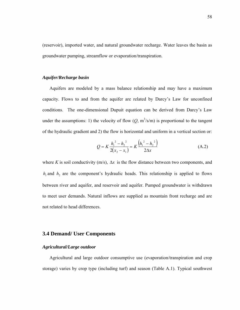
58
(reservoir), imported water, and natural groundwater recharge. Water leaves the basin as
groundwater pumping, streamflow or evaporation/transpiration.
Aquifer/Recharge basin
Aquifers are modeled by a mass balance relationship and may have a maximum
capacity. Flows to and from the aquifer are related by Darcy’s Law for unconfined
conditions. The one-dimensional Dupuit equation can be derived from Darcy’s Law
under the assumptions: 1) the velocity of flow (Q, m3/s/m) is proportional to the tangent
of the hydraulic gradient and 2) the flow is horizontal and uniform in a vertical section or:
( )( )
xhhK
xxhhKQ
∆−
=−
−=
22
22
21
12
22
21 (A.2)
where K is soil conductivity (m/s), x∆ is the flow distance between two components, and
1h and 2h are the component’s hydraulic heads. This relationship is applied to flows
between river and aquifer, and reservoir and aquifer. Pumped groundwater is withdrawn
to meet user demands. Natural inflows are supplied as mountain front recharge and are
not related to head differences.
3.4 Demand/ User Components
Agricultural/Large outdoor
Agricultural and large outdoor consumptive use (evaporation/transpiration and crop
storage) varies by crop type (including turf) and season (Table A.1). Typical southwest
59
US crops (Alfalfa, cotton, lettuce and wheat) are available to be selected in the model. An
override option allows users to provide data for alternative crops or a lumped water
demand for entire agricultural area. Large outdoor turf uses include schools, parks and
public and private golf courses. Golf course uses are further categorized by turf type (e.g.,
fairways versus greens). Consumptive use per acre of crop is computed by:
cropcropcrop ACUD = (A.3)
where cropD is a total crop consumptive use (m3/s), cropCU is consumptive use factor
(m3/s/m2), and cropA is crop acreage (m2).
Agricultural land retirement is provided as an option to remove land from production.
All outdoor uses (except lettuce crops) can accept reclaimed water or direct supply from a
source. Therefore, the priorities of which water should be used first or the proportion of
each water source must be user defined. Depending on the proportion selected, total
revenue against total cost varies (Table A.2). Required model parameters for the large
outdoor areas are listed in Table A.3.
Domestic
Domestic use is based on the area’s population and the number of households. Both
indoor and outdoor domestic uses are modeled in reasonable detail. Indoor water use
components are toilets, showers, faucets, evaporative coolers, clothes washers, bathtubs,
and dishwashers. In general, the use by each component is computed by:
NPUSENUD fixfixfix = (A.4)
60
where fixD is total fixture use per household per day, fixNU is number of fixture uses per
person per day, NP is number of persons per household, and fixUSE is water use per
fixture use.
Typical values for the number of fixture per household and its uses per day are given
in Table A.4. As seen, toilet water use is dependent on installation time. High efficiency
fixtures are assumed to be installed after 1990 while lower efficiency fixtures were
assumed to be installed prior to 1984. Thus, toilets are divided into three age groups,
before 1984, after 1990, and between 1984 and 1990. In the same manner, shower units
have two efficiencies which are low efficiency prior to 1994 and high efficiency after
1994. The total of all fixtures is the summed and scaled by the number of households. A
small percentage of indoor use is assumed to evaporate and the remainder is returned to a
WWTP. Grey water reuse is used first to meet a residence’s outdoor demand.
Outdoor residential water use consists of permanent irrigation water use, fountains,
and swimming pools. Permanent irrigation water use consists of turf watering and drip
irrigation. Outdoor use for irrigation is computed by an equation similar to Eq. A.3.
Swimming pool evaporation is estimated as the evaporation rate times the surface area of
the pool. Outdoor water monthly demand is reduced by the average monthly precipitation
depth. Irrigated areas, average pool size and the percentage of homes with pools and
fountains are user defined. Figure A.2 shows mass balance relationship through four
domestic areas.
Industrial
61
Industrial use is assumed to be proportional to the number of businesses in the study
area. The total water demand of industrial area is calculated as the sum of indoor and
outdoor water use for general commercial, car washes, and swimming pool uses. The
diversity of industry and their water use makes it difficult to develop more sophisticated
relationships. As defaults, eighty-five percent of industrial use is assumed to be an indoor
use and returned to the WWTP and the remainder considered as outdoor consumptive
use. The default average per business water use was estimated from billing records for
the Upper San Pedro subwatershed (Southern Arizona).
Environmental and recreational uses
Total water demand in environmental and recreational areas is the total consumptive
use of the area’s vegetation. Here, we limit the analysis to three trees (Cottonwood,
Tamarix, and Mesquite), grass and open water. Table A.5 lists the default consumptive
use for each category. The user supplies the areas of the comprising riparian area and the
percent of different trees (Table A.5). The use by each riparian category is computed by:
vegvegveg ACUD = (A.5)
where vegD is total riparian demand (m3/s), vegCU is consumptive use per acre (m3/s/m2),
and vegA is acreage of vegetation (m2).
Benefits of the riparian area in terms of fishing, float-boating, hiking, and camping
are assumed to be related to the streamflow and the area’s population. Default
relationships were developed by Stewart (personal communication, 2005) based on
compilations of riparian area economic evaluations from around the United States and
62
regional recreation statistics (Cordell, 1999). These benefits are intended to estimate the
economic value of riparian area but are site specific. Minimum required riparian flows
can be defined or an additional fee to preserve naturalness can be assessed.
3.5 Water Quality Transformations
Biochemical oxygen demand (BOD), total suspended solids (TSS), hardness and
Giardia are modeled as representative water quality indicators. An incremental
deterioration in water quality is assumed during each use. Two water and wastewater
treatment facility representations are available to model treatment of the four pollutants: a
lumped facility with an incremental change or representative removal efficiency and a
series of conventional unit processes with water quality changes based on literature
equations.
Users/Lumped treatment facilities
The lumped incremental improvement or removal efficiency model follows Ocanas
and Mays (1981a and b) in which water quality is improved by a constant increment (Eq.
A.6a) or related to the efficiency of a pollutant removal (Eq. A.6b):
( )∑
∑ ∆+=
out
ininout Q
CQC (A.6a)
( )
∑∑−
=out
ininout Q
CQC
η1 (A.6b)
63
where ∆ is amount of quality degradation (mg/l) and η is removal efficiency (%). Cin
and Cout are the contaminant concentrations in the treatment plant influent and effluent,
respectively.
Water quality degradation during use can be estimated as the difference between
WTP outflow and WWTP inflow concentrations from historical data and substituted as
∆ in Eq. A.6a. After use, wastewater is returned to a WWTP and simplified water and
wastewater treatment facilities adopt the lumped removal efficiency (Eq. A.6b). Input
parameters for lumped treatment facilities are listed in Table A.6.
Conventional water treatment plants
More complex WTP unit operation algebraic descriptions are available in literature
(Gummerman et al., 1979 and Reynolds, 1982). Each WTP is assumed to contain the
standard WTP unit processes; rapid mixing and chemical addition, flocculation,
disinfection with chlorine, sedimentation, filtration, and sludge handling using drying
beds (Figure A.3).
Capacities of the unit processes are dependent on the design flow (DF, m3/s) that is
assumed to be 1.5 times of inflow at the beginning of the simulation period. For example,
basin volume of rapid mixing (RV, m3) with a constant detention time (DT), 30 second,
is:
RV = DT DF (A.7)
Basin volume of flocculation (FV) is calculated by an assumption of a 30 minute
detention time (FDT) or:
64
DFFDTFV = (A.8)
The sedimentation basin is designed in a similar manner assuming the basin depth
(DEPTH) is 3.66m (12ft ) or:
DEPTH
DFSDTSAREA 4.5570= (A.9)
where SAREA is the total surface area of the sedimentation basin (m2) and SDT is the
detention time (5 hrs).
The filter surface area (FAREA) depends on the influent flow rate to filtration basin
from the sedimentation basin, FLOW3, or:
QAVE
ECFFLOWFAREA 34.694= (A.10)
where ECF is ratio of design flow and operation flow and QAVE is maximum allowable
average filtration rate (m3/s).
Water quality improvements occur in each unit process except during rapid mixing
that adversely affect TSS. Aluminum hydroxide (AlOH3, mg/l) is formed by injecting
alum in the rapid mixing basin and increases turbidity.
ALUMAlOHTSSTSS ininRM 26.0)( 3 ++= (A.11)
where TSSRM and TSSin are TSS concentrations in the effluent from and influent to the
rapid mixing unit, (AlOH3)in is the amount of AlOH3 included in natural inflow, assumed
as 0 mg/l, and ALUM is the injected amount of alum to the rapid mixing unit. The TSS
concentration during flocculation is constant and decreased in sedimentation and
filtration units corresponding to sedimentation tank overflow rate and the filter’s effective
sand size (0.5 mm).
65
Removal efficiencies of BOD and hardness are assumed to be the same for TSS. For
Giardia, the removal efficiencies during flocculation, disinfection, and filtration are 0.5
log (68.4 %), 0.5 log, and 2.0 log (99.0 %), respectively.
Table A.7 lists the input parameters for the above equations and the default values.
The total water treatment cost is the material and labor costs for construction and
maintenance (Smith, 1986).
Conventional wastewater treatment plant
The WWTP is modeled using the equations collected by Tang et al. (1984 and 1987).
These equations are based on unit operations in a conventional facility: primary settling,
aeration tank, secondary settling, gravity thickening, anaerobic primary digestion,
anaerobic secondary digestion, and vacuum filter (Figure A.4). The unit process sizes are
input to calculate the removal efficiency and cost of each unit. For simplicity, unlike
Tang et al., the recycling rate of water to the primary settling is fixed.
BOD and TSS are simulated using Tang’s equations. However, since relationships are
not available for hardness and Giardia, their removal efficiencies are assumed to be the
same as the lumped system. TSS is the sum of active biomass concentration, volatile
biodegradable suspended solids, fixed suspended solids, and volatile inert suspended
solids. Cost relationships include construction and operations and maintenance. Equation
parameters are listed in Table A.8.

66
4. APPLICATIONS
To demonstrate how the model can be used, three scenarios are considered on a
hypothetical system for a twenty year planning period (2000-2020). The first scenario
examines the impact of conservation measures aimed at reducing domestic and industrial
demands. The second condition represents the inability to secure additional external
water sources and its impact on long-term system storage. Finally, the cost effectiveness
and impact on water quality of decentralized treatment is analyzed for a disperse supply
system that covers a range of topography.
The hypothetical system is comprised of five sources (precipitation, imported water,
uncontrolled river, regulated river with reservoir, groundwater), twelve users (four
domestic areas, an industrial area, four agricultural areas, two large outdoor turf areas, an
environmental and recreational area), five treatment systems (two water treatment and
three wastewater treatment systems), and a recharge facility. Table A.9 lists the
population input parameters (initial population and growth rates).
Historical precipitation data from Coolidge, AZ was taken from the Arizona
Meteorological Network (AZMET) (http://ag.arizona.edu/azmet/.html) for the period of
1987 to 2004 (Figure A.5). As noted, precipitation provides flow into water sources such
as rivers, reservoirs, and the groundwater aquifer and is assumed to reduce outdoor water
demands for turf and agriculture.
A watershed (5,598 km) of San Pedro River from the Mexican Border through
Benson, AZ was used for calculating runoff. Runoff coefficients for the catchments area
was taken as 0.44 for average cultivated area (Chow et al. 1988. Table 15.1.1). Total soil
67
loss from catchments area was calculated as a constant rate 476.26 m3/km2/yr (1.0
af/mi2/yr) of drainage area (Branson et al. 1981, Figure 6-24). Only 0.5% of the soil loss
from the basin was assumed to contribute to TSS in inflows to the river and reservoir.
River flows can also be provided from upstream channel reaches. Historical flow data
from the Salt River, AZ (Figure A.6) was taken for this inflow from USGS NWIS web
data (http://waterdata.usgs.gov/nwis) for the period of 1987 to 2004. Inflow to reservoir
and outflow from reservoir was assumed as historical data at Roosevelt Dam in the Salt
River (Figure A.7) that were taken from USGS NWIS web data. Surface water sources
are connected with the underlying aquifer by Eq. A.2. Precipitation also infiltrates to the
aquifer.
Monthly historical data for 1987 to 2004 were converted to seasonal data and to a
time series that had the same statistical characteristics for the period of 2000 to 2020. The
imported water is limited to 1.956 m3/s (50 kafy). Controlled recharge is assumed to
occur through an infiltration basin that was modeled using Eq. A.2.
Table A.10 lists the layout and flow connections between the system components.
Open channel gravity flow transports untreated water when permitted to reduce cost.
However, pumping through pipelines is required in some cases such as extracting
agricultural irrigation water from groundwater. Pipe flow velocities are bounded to less
than 1.5 m/s (5 ft/s) by changing pipe diameters through trial and error by the author
before simulation. The leakage rate from distribution and sewer pipes is assumed to be 10
percent of the flow and evaporation from canals are included. Evaporation is 1.1
68
m/season (42.5 in/season) for the growing season, and for non-growing season, 0.5
m/season (9.62 in/season) or may be modified as is input.
Default agriculture water use is based upon Pima County, Tucson, AZ data (Table
A.1) and required inputs are the total acreages for each crop/turf area (Table A.2). The
cost and return for crops is computed on an annual basis. Unit yield, prices and costs are
listed in Table A.2. Water costs of new water (direct from a source) and reclaimed water
is $0.024 and $0.02 per m3 ($30 and $25 per acre-ft), respectively. If the flowrate in the
riparian zone/recreation area is less than 95% of the upstream flowrate, a fee of
$35/month per person in the basin is assessed to maintain the natural areas.
Water and wastewater treatment plant can be chosen as lumped or conventional
systems. Table A.9 shows the incremental removal efficiencies/degradations and the
water losses for the lumped treatment systems. Removal efficiencies in conventional
treatment systems are computed using the unit process Eqs. A.8 - A.12 and Tang
equations. Conventional systems were set as the default simulation. Contaminant
concentrations are assumed to be reduced by 30% during flow to the aquifer.
The following results presented in the following sections were developed by either
single model evaluations or extensive trial and error and engineering judgment. They are
not necessarily optimal solutions.

69
4.1 Scenario 1 – Effectiveness of Conservation Practices
Conservation practices are means to stretch current water supplies. Population growth
controls may also be employed to limit demand increases and to avoid constructing new
infrastructure and/or water supplies. Here, a scenario is posed in which a community
desires to examine the impact of these types of measures on the base condition described
above. Each measure (Table A.11) is initiated independently in 2012.
To reduce indoor use, incentives for (1) faucet, shower head, and toilet replacement
with more efficient fixtures and (2) front loading clothes washer purchases can be
provided. The amount of savings depends upon the age of the existing fixtures/appliance.
An annual government investment must be defined to implement the incentive program.
It is assumed that a $70 incentive will be provided per house and the total annual subsidy
is $100,000.
Generally outdoor use reductions are made by ordinance for new homes. For
example, new homes may be required to have a grey water reuse system in which water
from bathtubs, faucets, clothes washers, and showers is collected for outdoor purposes.
Grey water retrofit construction costs for existing homes are prohibitive. All of the above
measures will reduce demand for pumping but will also reduce the amount of reclaimed
water available for large area irrigation. Other ordinances can include prohibiting
fountains and evaporative coolers in new homes and requiring existing homes to remove
fountains.
Swimming pools are a major consumptive use. In the climate conditions of the
hypothetical community, the average evaporation loss from a swimming pool is about 5
70
m/yr (19 ft/year). Evaporation losses can be reduced by one or more set of measures. An
incentive program could be introduced for pool cover purchases that would be used in the
off-season. Other ordinances for reducing pool use are reducing pool draining
frequencies, restricting future swimming pools construction, filling existing swimming
pools, or reusing swimming pool drain or back-flush water as grey water.
Other water saving programs that can be evaluated are briefly described below.
During the growing season, outdoor water use restrictions prohibit irrigation on a
particular day or time by ordinance to reduce evaporation volumes. An irrigation
efficiency program will require efficiency gains from 75% to 90%. Landscaping
standards require turf irrigation systems to be replaced by drip irrigation or xeriscaping.
Rainfall harvesting can replace treated water usage to reduce outdoor water use in new or
existing homes. Lastly, a water wasting ordinance imposes fines for wasting or
unreasonable use of water. These losses are assumed to be zero after the ordinance
implement.
Similar conservative measures, such as toilet retrofit, improvement of water drip
irrigation efficiency, outdoor water use restriction, water loss due to violations and
swimming pool savings, can be applied to the industrial sector. Only purchasing pool
covers is supported with a government incentive. All other programs are implemented by
ordinance. In addition, water audits can be completed on these large users. An initial
investment for water audits is $4,000 with annual cost of $2,000 per year thereafter for 10
years and provides an expected 27,137 m3/yr (22 afy) of water savings.
71
Water demand before and after implementing conservation measures and other basic
input parameters are listed in Table A.12. Incentives have an annual cost for a program
and a cost per house (Table A.13). Table A.14 lists the effects of each of the conservation
measures on the total water supply system’s operation cost and water use savings in
domestic areas for the 20-year simulation period when implemented in year 2012.
Facility construction cost remains the same, while operation cost declines with respect to
water use decrease. Operational cost for pumping and piping is reduced as the amount of
water conveyance decrease. Some conservation measures decrease water use by reducing
demand through high efficient fixtures. Water and wastewater treatment operational cost
also decreases due to the water demand reduction. The other conservation programs
decrease fresh water usage by using reclaimed water through grey water recycling,
rainfall harvesting, or pool discharges, while water demands remain the same.
Removing turf and replacing with drip irrigation systems saves 9.2% of the water
demand (use as well) and total operation cost. Installing grey water reuse systems reduces
the total operation cost by 8.95% and the domestic use by 15.07%. As mentioned in
Table A.11, an incentive program such as for installing grey water reuse system incurs an
additional cost to the water provider. As a result of this expense, the cost savings
percentage is smaller than the water demand reduction percentage. The trends in water
demand at the Domestic Area 1 are shown in Figure A.8 for implementing grey water
reuse and clothes washer retrofit incentive programs.
Some conservation measures, such as reusing pool discharges and restricting outdoor
water use do not have any benefit on water and cost saving. For example, the volume of
72
pool discharge to wastewater treatment systems is small. Restricting outdoor water use
does not change the volume of water applied since turf water demands are not adjusted
although the irrigation efficiency is improved. Industrial conservation has similar, but
smaller effects (Table A.15) since 85% of the industrial water use is used for indoor
purposes.
When all conservation measures including the installation of rainwater harvesting
system on water supply are simultaneously implemented in 2012, the water use in the
domestic areas fluctuated based on the amount of precipitation and decreased by more
than 70% (Figure A.9 and Table A.16). Total system cost, however, only decreases by
2.6% (Figure A.10). This decrease is not significant to a long-term water management
plan. However, because the primary goal of the plan is ordinarily safe-yield, the positive
effect on groundwater storage is a 0.9% increase over time as a result of increasing
population (Table A.16).
4.2 Scenario 2 – Unavailability of Supply Sources
As water resources become more stressed and climatic variability increases, the
potential for reduced supply is more likely. In addition, environmental systems may also
require additional water. In this scenario, it is assumed that the imported water source is
no longer available and that the existing use of reclaimed water as the riparian zone’s
water source precludes its use for other purposes. Serious repercussions are anticipated in
the water balance and groundwater mining must occur.
73
The main imported and reclaimed water use is agricultural. Average seasonal
consumptive use of each agricultural area is 0.063 km3/yr (51.30 kafy) and 0.114 km3/yr
(92.36 kafy) for growing and non-growing seasons, respectively. About 16% of
consumptive use during growing season is supplied from imported water (0.010 km3/yr)
and reclaimed water (0.009 km3/yr) under the base scenario that is defined as both
imported and reclaimed water are available. Figure A.11 shows the sources providing
water to Agricultural Area 1. The total amount of water from imported water and
reclaimed water to the four agricultural areas are 0.030 km3/yr and 0.034 km3/yr,
respectively.
Groundwater is used to replace the unavailable supplies for three cases: without
imported water, without reclaimed water, and without imported and reclaimed waters.
Figure A.12 shows the resulting groundwater storage change. Nearly 19% of the
groundwater storage is depleted when imported and reclaimed waters were not available
(Table A.17) demonstrating the need in many communities for these supplies in order to
maintain a sustainable system.
4.3 Scenario 3 – Decentralized Treatment
Decentralized wastewater treatment has become a topic of interest as a cost effective
means to treat and recycle effluent. For small communities, unsewered communities, and
communities covering a range of elevations, cluster wastewater treatment system, also
known as community-wide decentralized wastewater management, may be an appropriate
74
treatment option. The Minnesota Pollution Control Agency (2000) and Otis (2004)
investigated and described the need of wastewater treatment system in unsewered areas
and the benefits of decentralized wastewater treatment systems. They described a cluster
system as a wastewater collection, treatment and disposal systems that serves a small
number of units.
Here, we consider a distributed wastewater scheme in which multiple satellite
WWTPs are located throughout a community with the ability to treat and distribute
reclaimed water to nearby users (Figure A.13). The configuration is based on a dispersed
urban-suburban community with a maximum population of about 1.2 million. Economies
of scale suggest that, under many conditions, a single large WWTP would be less
expensive than multiple plants. However, when the community covers a range of
elevations and/or a large area, pumping and piping costs for reclaimed water may be
more expensive than construction cost of multiple wastewater treatment plants.
The efficacy of constructing up to two water treatment systems and three wastewater
treatment systems in the hypothetical system is examined in this application. Costs are
computed for treatment plant construction and operation, pumping and piping for water
transfers, system expansion, operation and maintenance of treatment system and energy
needed for pumping. Pipes between sources, treatment systems, and users were assumed
to be laid to cover the least distance and elevation and determined by a trial and error and
engineering judgment.
Cost and treatment capacities
75
Table A.18 lists the links and treatment facilities for the eight different combinations
compared with the base condition that is defined as two water treatment systems and
three wastewater treatment systems (Table A.10).
Results for one centralized and two decentralized lumped water treatment systems are
shown in Figure A.14. In the two WTP case, water treatment system 1’s capacity is not
increased from its initial size of 0.033 km3/yr while water treatment system 2 is expanded
from a capacity of 0.154 km3/yr to 0.296 km3/yr. When only one centralized WTP is
permitted, its capacity is equal to 0.187 km3/yr to 0.330 km3/yr (conditions 1 and 2 in
Table A.18).
The wastewater treatment system is more complicated as each type of wastewater
treatment system has six alternative wastewater treatment system combinations
(conditions 3 ~ 8 from Table A.18) on each lumped or conventional WWTP
representations. Figure A.15 shows the required simplified treatment plant capacity over
time for one centralized and three decentralized plants (base condition). Unit process
capacities for the one centralized wastewater treatment system alternative are shown in
Figure A.16 as a function of the surface area.
Tables A.19 and A.20 give detailed plant and unit operation capacities for all six
combinations of lumped and conventional system models, respectively. Since these
alternatives do not affect use, the sum of the plant capacities from multiple plant systems
is the same as for the single system.
Figure A.17 shows the total cost change over the planning period for conventional
and lumped treatment system representations, while Table A.21 lists the total cost in
76
present values, annual cost, and cost differences for the different treatment systems. As
shown in Figure A. 17, total cost jumps every five years because of system construction
and expansion. Lumped construction and operation cost (293.4×10⁶ $/yr, for the base
condition) for treatment systems appear to be overestimated compared to conventional
representations (242.4×10⁶ $/yr, for the base condition). However, the optimal treatment
distribution in this example for both lumped and conventional cases was 2 WTPs and 3
WWTPs. Finally, Table A.22 lists construction, expansion, and operation cost of all
components for all conditions for conventional and simplified treatment plant
representations. Since the transportation cost is dominated by piping/pumping, a remote
system is much more expensive.
The overriding factor in the cost effectiveness of multiple treatment plants is the cost
for transporting water through the system. These costs are determined by the distance and
elevation changes in the region. As seen in Table A.22, the operations and maintenance
costs for pumping when few plants were used was significant compared to treatment
costs. Therefore, construction of two water treatment plants and three wastewater
treatment plants (base condition in Table A.18) is the least expensive treatment system
for the community.
Water quality
Differences in water quality are examined between plant alternatives at key locations
and within the system for one plant configuration. Table A.23 lists the removal
efficiencies for the conventional and lumped WTP and WWTP models. In the unit
77
operation models for conventional systems, removal efficiencies are dependent upon the
influent water quality. Hence, values in Table A.23 are average removal efficiencies from
the total process.
Figure A.18 shows BOD and TSS level changes in the major water sources. Reservoir
water quality is stable over the period, while the river fluctuates with the discharge. The
TSS level in groundwater improves over the time as a result of continuous recharge of
clean reclaimed water. If credit is received for treatment during recharge, costs can be
reduced by increasing aquifer recharge. Pollutant concentrations in the river and reservoir
(Figures A.18 and A.19) remain relatively constant over time, however groundwater
contamination of all four pollutants are reduced.
Figures A.20, A.21, and A.22 show effluent water quality of BOD and TSS,
hardness, and Giardia from each user. Since water quality deterioration is assumed to be
constant over the time for a given user type, the effluent quality does not change.
Agricultural water demands usually show significant seasonal variations depending on
the crop growing season. Reclaimed water for irrigation may contain high mineral
content and Giardia levels. Giardia levels in the groundwater are maintained below 1/ml:
making it a suitable domestic source.
5. CONCLUSIONS
Given the complexity of water supply systems, decision makers may have difficulty
understanding the impact of water management policies. To understand the impact of
78
decisions, a modular water system simulation model has been developed. The modular
structure allows a general system model to be constructed with minimal effort. Model
components include detailed domestic indoor and outdoor usage, industrial, agricultural,
and environmental demands, multiple supplies, conveyance between sources and demand
centers, and surface and groundwater storage. Since water quality plays a key role in
water management, it is modeled through the system including water and wastewater
treatment representations. Simulation is performed on seasonal time steps with decisions
at critical periods. Costs are estimated for new infrastructure (conveyance, recharge, or
treatment facilities), water usage, and the implementation of conservation practices.
A series of applications demonstrate the ability to examine the impacts of external
factors and to assist in making a range of decisions. The first application showed the
relative impacts of a set of conservation measures on the water demand and consumptive
use. These results would assist decision makers in determining the utility of
implementing the measures, the general public in understanding their value and both
groups in developing a consensus on accepting the plans. The loss of water sources is
examined in the second application to demonstrate its implications on long-term storage
and system sustainability.
A large spatially distributed system is considered in the final example to evaluate the
potential of distributed water and wastewater treatment. Costs for alternative system
designs were determined using engineering judgment and trial and error. The results
show that the distance and elevation changes between demand centers in the example

79
system are such that multiple distributed treatment facilities are more cost effective than
single centralized plants.
Three primary extensions of the present level of modeling are recommended. To be a
useful practical tool, the models should be accessible through the internet so the entire
community can perform simulations. Second, in the applications here the resulting
decisions were made based on engineering judgment, these modules should be linked
with optimization routines. Lastly, additional modules should be developed to extend the
model capabilities. These components can be combined in the present structure and
provide more detailed descriptions of unit operation processes.
80
6. REFERENCES
Ahmad, S., and Simonovic, S. P. (2000). “System dynamics modeling of reservoir
operations for flood management.” Journal of Computing in Civil
Engineering, 14(3), 190-198.
Biddle, S. H. (2001). “Optimizing the TVA reservoir system using RiverWare, bridging
the gap: meeting the world’s water and environmental resources challenges.”
Proceedings of the World Water and Environmental Resources Congress,
ASCE.
Branson, F. A., Gifford, G. F., Renard, K. G., and Hadley, R. F. (1981). Rangeland
hydrology, range science series 1. Society For Range Management, Denver,
CO.
Cai, X., Mckinney, D. C., and Lasdon, L. S. (2001). “Piece-by-Piece approach to solving
large nonlinear water resources management models.” Journal of Water
Resources Planning and management, 127(6), 363-368.
Cai, X., McKinney, D. C., and Lasdon, L. S (2003). “Integrated hydrologic-agronomic-
economic model for river basin management.” Journal of Water Resources
Planning and Management, 129(1), 4-16.
Chow, V. T., Maidment, D. and Mays, L. (1988). Applied hydrology. McGraw-Hill Book
Co. Singapore.
81
Cohen, D., Shamir, U., and Sinai, G. (2004). “Sensitivity analysis of optimal operation of
irrigation supply systems with water quality considerations.” Irrigation and
Drainage Systems, 18, 227-253.
Cordell, H. Ken (1999). Outdoor recreation in American life. A national assessment of
demand and supply trends. Sagamore Publishing.
Ejeta, M. Z., McGuckin, T., and Mays, L. W. (2004). “Market exchange impact on water
supply planning with water quality.” Journal of Water Resources Planning
and Management, 130(6), 439-449.
Erie, L. L, French, O. F., Bucks, D.A., and Harris, K. (1982). Consumptive use of major
crops in the Southwestern United States. USDA-ARS Conservation Research
Report Number 29.
Fulp, T. and Harkins, J. (2001). “Policy analysis using RiverWare: Colorado river interim
surplus guidelines.” Proceedings of ASCE World Water & Environmental
Resource Congress, Orlando, FL.
Gilmore, A., Magee, T., Fulp, T., and Strezepek, K. (2000). “Multi-objective
optimization of the Colorado river.” Proceedings of the ASCE 2000 Joint
Conference on Water Resources Engineering and Water Resources Planning
and Movement, Minneapolis, MN.
Gummerman, R. C., Russell, L. C, and Sigurd, P. H. (1979). Estimating water treatment
costs. EPA-600/2-79-162a. Cincinnati, OH.
82
Huang, G. H. and Loucks, D. P. (2000). “An inexact two-stage stochastic programming
model for water resources model for water resources management under
uncertainty.” Civil Engineering and Environmental Systems, 17(2), 95-118.
Loucks, D. P. (1995). “Developing and implementing decision support systems: a
critique and a challenge.” Water Resources Bulletin, 31(4), 571-582.
Magee, T. M. and Goranflo, H., M. (2002). “Optimizing daily reservoir scheduling at
TVA with RiverWare.” Proceedings of the Second Federal Interagency
Hydrologic Modeling Conference, Las Vegas, NV.
Minnesota Pollution Control Agency. (2000). Wastewater Treatment and Collection
Systems.
Nandalal, K. D. W., and Simonovic, S. P. (2003). “Resolving conflicts in water sharing: a
systemic approach.” Water Resources Research, 39(12), 1362-1372.
Ocanas, G. and Mays, L. W. (1981a). “A model for water reuse planning.” Water
Resources Research, 17(1), 25-32.
Ocanas, G. and Mays, L. W. (1981b). “Water reuse planning models: extensions and
applications.” Water Resources Research, 17(5), 1311-1327.
Otis, R. J. (2004). “Unsewered communities: paralyzed by disparate regulatory
programs?” 2004 Onsite Conference X in Sacramento, 21-24 March 2004,
ASAE.
Palmer, R. N, Wright, J. R., Smith, J. A., Cohon, J. L., and ReVelle, C. S. (1980). Policy
analysis of reservoir operation in the Potomac River Basin, Volume I,
executive summary, Johns Hopkins University, Baltimore, MD.
83
Palmer, R. N, Keyes, A., and Fisher, S. (1993). “Empowering stakeholders through
simulation in water resources planning.” Proceedings of the ASCE Water
Management in the 90s Conference, Seattle, Washington, 451-454
Palmer, R. N., Mohammadi, A., Hahn, M. A., Kessler, D., Dvorak, J. V., and Parkinson,
D. (2000). “Computer assisted decision support system for high level
infrastructure master planning: case of the city of Portland Supply and
Transmission Model (STM).” Proceedings of the ASCE 2000 Joint
Conference on Water Resources Engineering and Water Resources Planning
and Movement, Minneapolis, MN.
Passell, H., Tidwell, V. and Webb, E. (2002). “Cooperative modeling: a tool for
community-based water resource management.” Southwest Hydrology, 1(4),
26.
Reynolds, T. D. (1982). Unit operations and processes in environmental engineering,
PWS Publishers, B/C Engineering Division, Boston, Massachusetts.
Ruth, M. and Pieper, F. (1994). “Modeling spatial dynamics of sea-level rise in a coastal
area.” System Dynamics Review, 10(4), 375-389.
Simonovic, S. P. and Bender, M. J. (1996). “Collaborative planning-support system: an
approach for determining evaluation criteria.” Journal of Hydrology, 177,
237-251.
Simonovic, S. P., Fahmy, H., and El-shorbagy, A. (1997). “The use of object-oriented
modeling for water resources planning in Egypt.” Water Resources
Management, 11, 243-261.
84
Simonovic, S. P. and Fahmy, H. (1999). “A new modeling approach for water resources
policy analysis.” Water Resources Research, 35(1), 295-304.
Smith, R. (1986). Computer assisted preliminary design for drinking water treatment
process systems. U.S. Environmental Protection Agency, Washington, D.C.,
EPA/600/2-86/007A (NTIS PB86181112).
Sumer, D. Y., Lansey, K. and Richter, H. (2004). “Evaluation of conservation measures
in the Upper San Pedro Basin.” The 2004 World Water and Environmental
Resources Congress, Salt Lake City, UT, ASCE.
Stave, K. A. (2003). “A system dynamics model to facilitate public understanding of
water management options in Las Vegas, Nevada.” Journal of Environmental
Management, 67, 303-313.
Tang, C. C., Brill, E. D., and Pfeffer, J. T. (1984). Mathematical models and optimization
techniques for use in analysis and design of wastewater treatment systems,
Research Report No. 194, Water Resources Center, University of Illinois at
Urbana-Champaign, Urbana, Ill.
Tang, C. C., Brill, E. D., and Pfeffer, J. T. (1987). “Optimization techniques for
secondary wastewater treatment system.” Journal of Environmental
Engineering, 113(5), 935 – 951.
US Army Corps of Engineers (2003). HEC-ResSim User’s Manual, V. 2, September.
(www.hec.usace.army.mil/software/hec-ressim/hecressim-hecressim.htm)
U.S. Bureau of Reclamation (1987). Colorado river simulation system: overview.
Denver, Colorado.
85
US EPA (1976). Areawide assessment procedures manual. Appendix H. EPA 600/9-76-
014. Cincinnati, OH.
Wurbs, R. A. (1993). “Reservoir system simulation and optimization models.” Journal of
Water Resources Planning and Management, 119(4), 455-472.
Yang, S., Sun, Y., and Yeh, W. W-G. (2000). “Optimization of regional water
distribution system with blending requirements.” Journal of Water Resources
Planning and Management, 126(4), 229-235.
Yen, K. H., and Chen, C. Y. (2001). “Allocation strategy analysis of water resources in
South Taiwan.” Water Resources Management, 15, 283-297.
Zagona, E. A., Fulp, T. J., Shane, R., Magee, T., and Goranflo, H. M. (2001).
“Riverware: a generalized tool for complex reservoir system modeling.”
Journal of the American Water Resources Association, 37(4), 913-929.
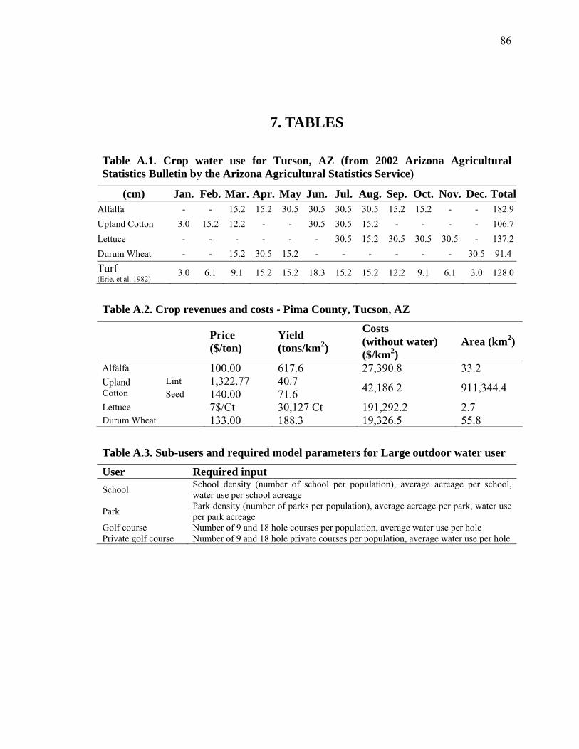
86
7. TABLES
Table A.1. Crop water use for Tucson, AZ (from 2002 Arizona Agricultural Statistics Bulletin by the Arizona Agricultural Statistics Service)
(cm) Jan. Feb. Mar. Apr. May Jun. Jul. Aug. Sep. Oct. Nov. Dec. TotalAlfalfa - - 15.2 15.2 30.5 30.5 30.5 30.5 15.2 15.2 - - 182.9Upland Cotton 3.0 15.2 12.2 - - 30.5 30.5 15.2 - - - - 106.7Lettuce - - - - - - 30.5 15.2 30.5 30.5 30.5 - 137.2Durum Wheat - - 15.2 30.5 15.2 - - - - - - 30.5 91.4 Turf (Erie, et al. 1982) 3.0 6.1 9.1 15.2 15.2 18.3 15.2 15.2 12.2 9.1 6.1 3.0 128.0
Table A.2. Crop revenues and costs - Pima County, Tucson, AZ
Price ($/ton)
Yield (tons/km2)
Costs (without water) ($/km2)
Area (km2)
Alfalfa 100.00 617.6 27,390.8 33.2 Upland Cotton
Lint 1,322.77 40.7 42,186.2 911,344.4 Seed 140.00 71.6 Lettuce 7$/Ct 30,127 Ct 191,292.2 2.7 Durum Wheat 133.00 188.3 19,326.5 55.8
Table A.3. Sub-users and required model parameters for Large outdoor water user
User Required input School School density (number of school per population), average acreage per school,
water use per school acreage
Park Park density (number of parks per population), average acreage per park, water use per park acreage
Golf course Number of 9 and 18 hole courses per population, average water use per hole Private golf course Number of 9 and 18 hole private courses per population, average water use per hole
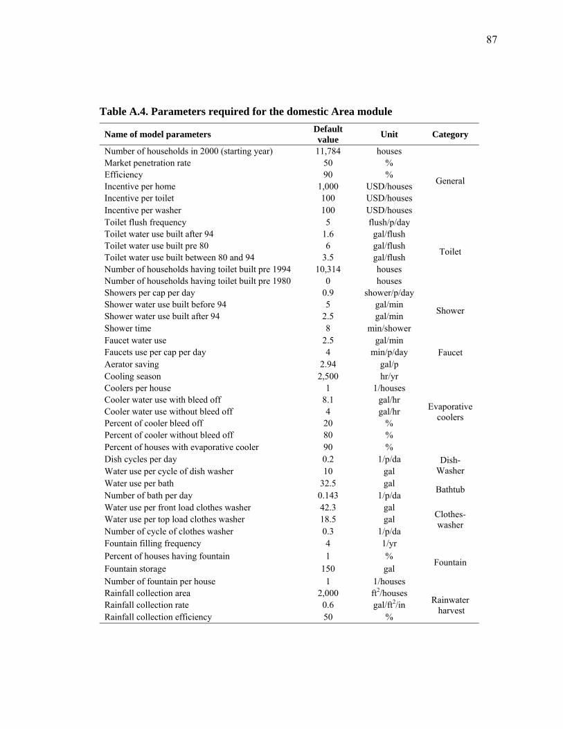
87
Table A.4. Parameters required for the domestic Area module
Name of model parameters Default value Unit Category
Number of households in 2000 (starting year) 11,784 houses
General
Market penetration rate 50 % Efficiency 90 % Incentive per home 1,000 USD/houses Incentive per toilet 100 USD/houses Incentive per washer 100 USD/houses Toilet flush frequency 5 flush/p/day
Toilet
Toilet water use built after 94 1.6 gal/flush Toilet water use built pre 80 6 gal/flush Toilet water use built between 80 and 94 3.5 gal/flush Number of households having toilet built pre 1994 10,314 houses Number of households having toilet built pre 1980 0 houses Showers per cap per day 0.9 shower/p/day
Shower Shower water use built before 94 5 gal/min Shower water use built after 94 2.5 gal/min Shower time 8 min/shower Faucet water use 2.5 gal/min
Faucet Faucets use per cap per day 4 min/p/day Aerator saving 2.94 gal/p Cooling season 2,500 hr/yr
Evaporative coolers
Coolers per house 1 1/houses Cooler water use with bleed off 8.1 gal/hr Cooler water use without bleed off 4 gal/hr Percent of cooler bleed off 20 % Percent of cooler without bleed off 80 % Percent of houses with evaporative cooler 90 % Dish cycles per day 0.2 1/p/da Dish-
Washer Water use per cycle of dish washer 10 gal Water use per bath 32.5 gal
Bathtub Number of bath per day 0.143 1/p/da Water use per front load clothes washer 42.3 gal
Clothes- washer Water use per top load clothes washer 18.5 gal
Number of cycle of clothes washer 0.3 1/p/da Fountain filling frequency 4 1/yr
Fountain Percent of houses having fountain 1 % Fountain storage 150 gal Number of fountain per house 1 1/houses Rainfall collection area 2,000 ft2/houses
Rainwater harvest Rainfall collection rate 0.6 gal/ft2/in
Rainfall collection efficiency 50 %
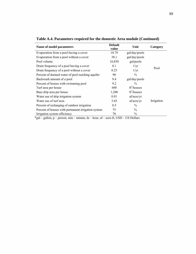
88
Table A.4. Parameters required for the domestic Area module (Continued)
Name of model parameters Default value Unit Category
Evaporation from a pool having a cover 18.79 gal/day/pools
Pool
Evaporation from a pool without a cover 38.1 gal/day/pools Pool volume 16,830 gal/pools Drain frequency of a pool having a cover 0.1 1/yr Drain frequency of a pool without a cover 0.25 1/yr Percent of drained water of pool reaching aquifer 90 % Backwash amount of a pool 9.4 gal/day/pools Percent of houses with swimming pool 9.2 % Turf area per house 600 ft2/houses
Irrigation
Base drip area per house 1,200 ft2/houses Water use of drip irrigation system 0.91 af/acre/yr Water use of turf area 3.65 af/acre/yr Percent of recharging of outdoor irrigation 0.5 % Percent of houses with permanent irrigation system 75 % Irrigation system efficiency 70 %
*gal – gallon, p – person, min – minute, hr – hour, af – acre-ft, USD – US Dollars
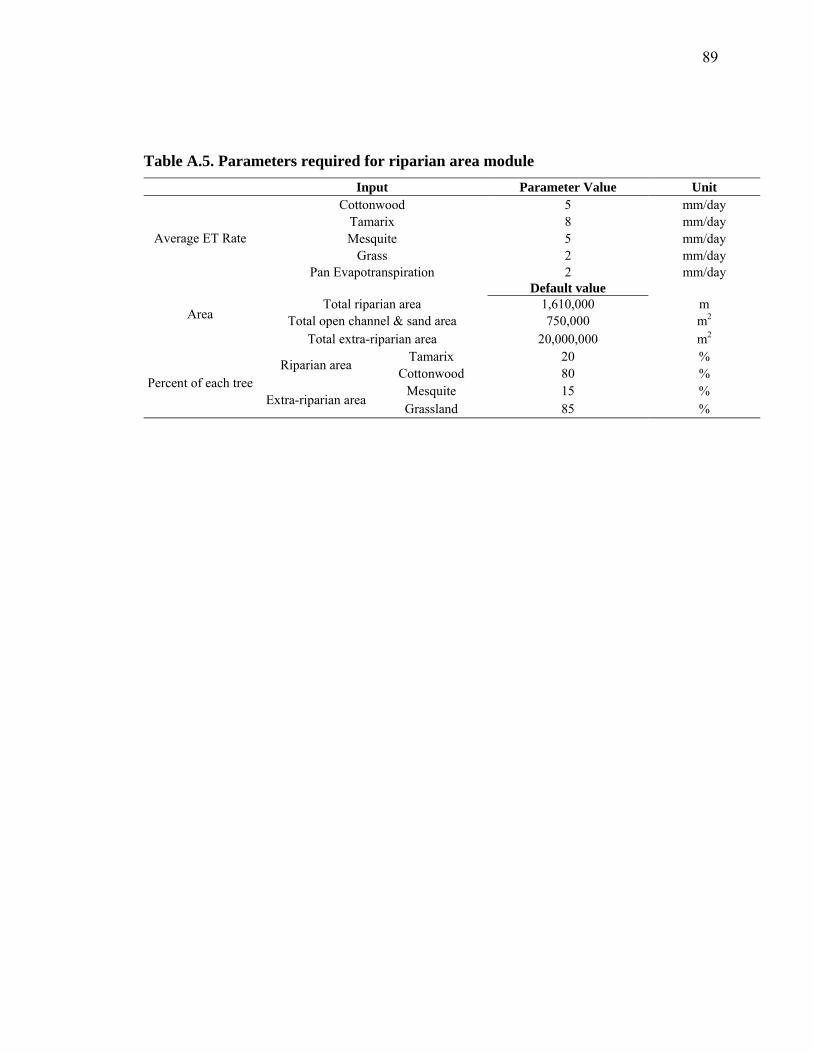
89
Table A.5. Parameters required for riparian area module Input Parameter Value Unit
Average ET Rate
Cottonwood 5 mm/day Tamarix 8 mm/day Mesquite 5 mm/day
Grass 2 mm/day Pan Evapotranspiration 2 mm/day
Area
Default value Total riparian area 1,610,000 m
Total open channel & sand area 750,000 m2 Total extra-riparian area 20,000,000 m2
Percent of each tree Riparian area Tamarix 20 %
Cottonwood 80 %
Extra-riparian area Mesquite 15 % Grassland 85 %
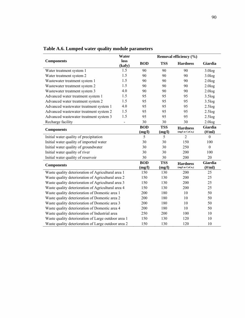
90
Table A.6. Lumped water quality module parameters
Components Water
loss (kafy)
Removal efficiency (%)
BOD TSS Hardness Giardia
Water treatment system 1 1.5 90 90 90 3.0log Water treatment system 2 1.5 90 90 90 3.0log Wastewater treatment system 1 1.5 90 90 90 2.0log Wastewater treatment system 2 1.5 90 90 90 2.0log Wastewater treatment system 3 4.0 90 90 90 2.0log Advanced water treatment system 1 1.5 95 95 95 3.5log Advanced water treatment system 2 1.5 95 95 95 3.5log Advanced wastewater treatment system 1 4.0 95 95 95 2.5log Advanced wastewater treatment system 2 1.5 95 95 95 2.5log Advanced wastewater treatment system 3 1.5 95 95 95 2.5log Recharge facility - 30 30 30 2.0log
Components BOD (mg/l)
TSS (mg/l)
Hardness (mg/l as CaCo3)
Giardia (#/ml)
Initial water quality of precipitation 5 5 2 0 Initial water quality of imported water 30 30 150 100 Initial water quality of groundwater 30 30 250 0 Initial water quality of river 30 30 200 100 Initial water quality of reservoir 30 30 200 20
Components BOD (mg/l)
TSS (mg/l)
Hardness (mg/l as CaCo3)
Giardia (#/ml)
Waste quality deterioration of Agricultural area 1 150 130 200 25 Waste quality deterioration of Agricultural area 2 150 130 200 25 Waste quality deterioration of Agricultural area 3 150 130 200 25 Waste quality deterioration of Agricultural area 4 150 130 200 25 Waste quality deterioration of Domestic area 1 200 180 10 50 Waste quality deterioration of Domestic area 2 200 180 10 50 Waste quality deterioration of Domestic area 3 200 180 10 50 Waste quality deterioration of Domestic area 4 200 180 10 50 Waste quality deterioration of Industrial area 250 200 100 10 Waste quality deterioration of Large outdoor area 1 150 130 120 10 Waste quality deterioration of Large outdoor area 2 150 130 120 10
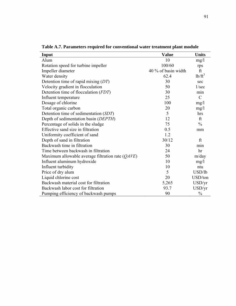
91
Table A.7. Parameters required for conventional water treatment plant module
Input Value Units Alum 10 mg/l Rotation speed for turbine impeller 100/60 rps Impeller diameter 40 % of basin width ft Water density 62.4 lb/ft3 Detention time of rapid mixing (DT) 30 sec Velocity gradient in flocculation 50 1/sec Detention time of flocculation (FDT) 30 min Influent temperature 25 C Dosage of chlorine 100 mg/l Total organic carbon 20 mg/l Detention time of sedimentation (SDT) 5 hrs Depth of sedimentation basin (DEPTH) 12 ft Percentage of solids in the sludge 75 % Effective sand size in filtration 0.5 mm Uniformity coefficient of sand 1.2 Depth of sand in filtration 30/12 ft Backwash time in filtration 30 min Time between backwash in filtration 24 hr Maximum allowable average filtration rate (QAVE) 50 m/day Influent aluminum hydroxide 10 mg/l Influent turbidity 10 ntu Price of dry alum 5 USD/lb Liquid chlorine cost 20 USD/tonBackwash material cost for filtration 5,265 USD/yr Backwash labor cost for filtration 93.7 USD/yr Pumping efficiency of backwash pumps 90 %
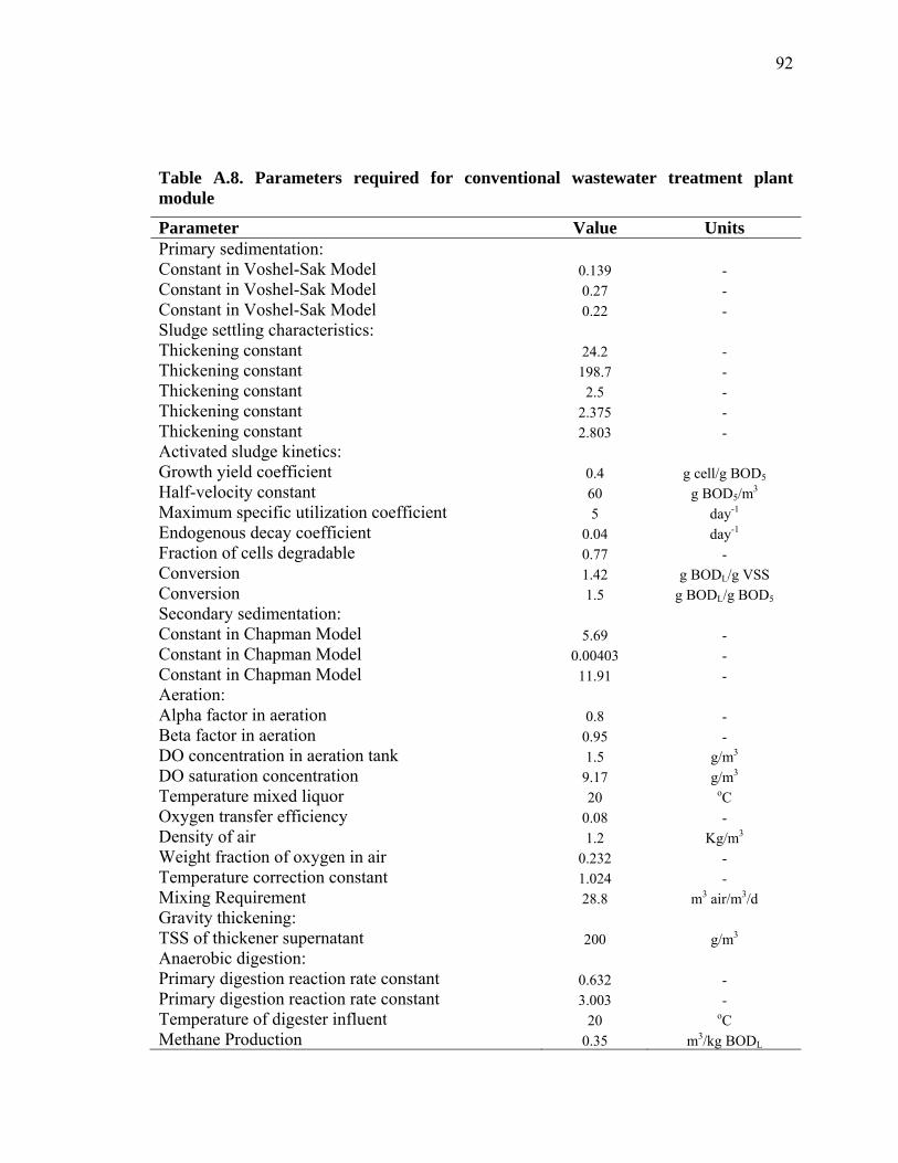
92
Table A.8. Parameters required for conventional wastewater treatment plant module
Parameter Value Units Primary sedimentation: Constant in Voshel-Sak Model 0.139 - Constant in Voshel-Sak Model 0.27 - Constant in Voshel-Sak Model 0.22 - Sludge settling characteristics: Thickening constant 24.2 - Thickening constant 198.7 - Thickening constant 2.5 - Thickening constant 2.375 - Thickening constant 2.803 - Activated sludge kinetics: Growth yield coefficient 0.4 g cell/g BOD5 Half-velocity constant 60 g BOD5/m3 Maximum specific utilization coefficient 5 day-1 Endogenous decay coefficient 0.04 day-1 Fraction of cells degradable 0.77 - Conversion 1.42 g BODL/g VSS Conversion 1.5 g BODL/g BOD5 Secondary sedimentation: Constant in Chapman Model 5.69 - Constant in Chapman Model 0.00403 - Constant in Chapman Model 11.91 - Aeration: Alpha factor in aeration 0.8 - Beta factor in aeration 0.95 - DO concentration in aeration tank 1.5 g/m3 DO saturation concentration 9.17 g/m3 Temperature mixed liquor 20 oC Oxygen transfer efficiency 0.08 - Density of air 1.2 Kg/m3 Weight fraction of oxygen in air 0.232 - Temperature correction constant 1.024 - Mixing Requirement 28.8 m3 air/m3/d Gravity thickening: TSS of thickener supernatant 200 g/m3 Anaerobic digestion: Primary digestion reaction rate constant 0.632 - Primary digestion reaction rate constant 3.003 - Temperature of digester influent 20 oC Methane Production 0.35 m3/kg BODL
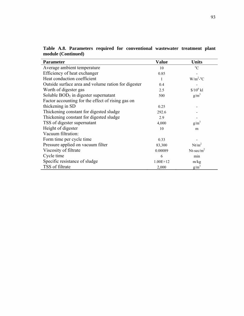
93
Table A.8. Parameters required for conventional wastewater treatment plant module (Continued)
Parameter Value Units Average ambient temperature 10 oC Efficiency of heat exchanger 0.85 - Heat conduction coefficient 1 W/m2-oC Outside surface area and volume ration for digester 0.4 - Worth of digester gas 2.5 $/106 kl Soluble BOD5 in digester supernatant 500 g/m3 Factor accounting for the effect of rising gas on thickening in SD 0.25 - Thickening constant for digested sludge 292.6 - Thickening constant for digested sludge 2.9 - TSS of digester supernatant 4,000 g/m3 Height of digester 10 m Vacuum filtration: Form time per cycle time 0.33 - Pressure applied on vacuum filter 83,300 Nt/m2 Viscosity of filtrate 0.00089 Nt-sec/m2 Cycle time 6 min Specific resistance of sludge 1.00E+12 m/kg TSS of filtrate 2,000 g/m3
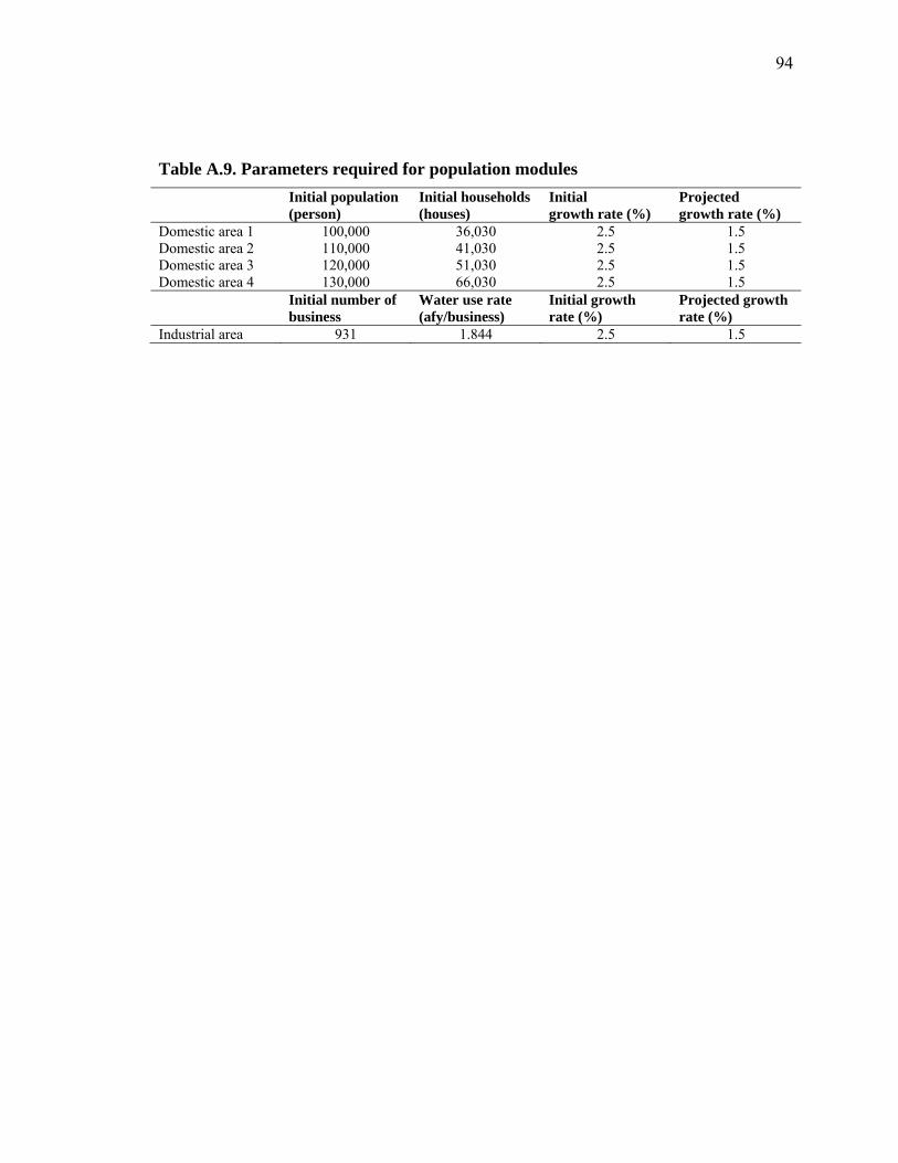
94
Table A.9. Parameters required for population modules Initial population
(person) Initial households (houses)
Initial growth rate (%)
Projected growth rate (%)
Domestic area 1 100,000 36,030 2.5 1.5 Domestic area 2 110,000 41,030 2.5 1.5 Domestic area 3 120,000 51,030 2.5 1.5 Domestic area 4 130,000 66,030 2.5 1.5 Initial number of
business Water use rate (afy/business)
Initial growth rate (%)
Projected growth rate (%)
Industrial area 931 1.844 2.5 1.5
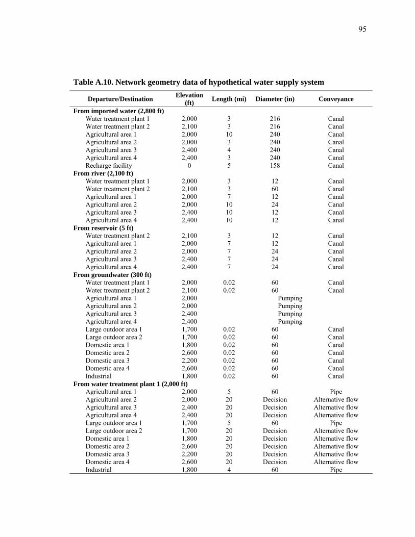
95
Table A.10. Network geometry data of hypothetical water supply system
Departure/Destination Elevation (ft) Length (mi) Diameter (in) Conveyance
From imported water (2,800 ft) Water treatment plant 1 2,000 3 216 Canal Water treatment plant 2 2,100 3 216 Canal Agricultural area 1 2,000 10 240 Canal Agricultural area 2 2,000 3 240 Canal Agricultural area 3 2,400 4 240 Canal Agricultural area 4 2,400 3 240 Canal Recharge facility 0 5 158 Canal
From river (2,100 ft) Water treatment plant 1 2,000 3 12 Canal Water treatment plant 2 2,100 3 60 Canal Agricultural area 1 2,000 7 12 Canal Agricultural area 2 2,000 10 24 Canal Agricultural area 3 2,400 10 12 Canal Agricultural area 4 2,400 10 12 Canal
From reservoir (5 ft) Water treatment plant 2 2,100 3 12 Canal Agricultural area 1 2,000 7 12 Canal Agricultural area 2 2,000 7 24 Canal Agricultural area 3 2,400 7 24 Canal Agricultural area 4 2,400 7 24 Canal
From groundwater (300 ft) Water treatment plant 1 2,000 0.02 60 Canal Water treatment plant 2 2,100 0.02 60 Canal Agricultural area 1 2,000 Pumping Agricultural area 2 2,000 Pumping Agricultural area 3 2,400 Pumping Agricultural area 4 2,400 Pumping Large outdoor area 1 1,700 0.02 60 Canal Large outdoor area 2 1,700 0.02 60 Canal Domestic area 1 1,800 0.02 60 Canal Domestic area 2 2,600 0.02 60 Canal Domestic area 3 2,200 0.02 60 Canal Domestic area 4 2,600 0.02 60 Canal Industrial 1,800 0.02 60 Canal
From water treatment plant 1 (2,000 ft) Agricultural area 1 2,000 5 60 Pipe Agricultural area 2 2,000 20 Decision Alternative flow Agricultural area 3 2,400 20 Decision Alternative flow Agricultural area 4 2,400 20 Decision Alternative flow Large outdoor area 1 1,700 5 60 Pipe Large outdoor area 2 1,700 20 Decision Alternative flow Domestic area 1 1,800 20 Decision Alternative flow Domestic area 2 2,600 20 Decision Alternative flow Domestic area 3 2,200 20 Decision Alternative flow Domestic area 4 2,600 20 Decision Alternative flow Industrial 1,800 4 60 Pipe
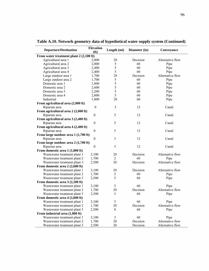
96
Table A.10. Network geometry data of hypothetical water supply system (Continued)
Departure/Destination Elevation (ft) Length (mi) Diameter (in) Conveyance
From water treatment plant 2 (2,100 ft) Agricultural area 1 2,000 20 Decision Alternative flow Agricultural area 2 2,000 5 60 Pipe Agricultural area 3 2,400 5 60 Pipe Agricultural area 4 2,400 5 60 Pipe Large outdoor area 1 1,700 20 Decision Alternative flow Large outdoor area 2 1,700 5 60 Pipe Domestic area 1 1,800 5 60 Pipe Domestic area 2 2,600 5 60 Pipe Domestic area 3 2,200 5 60 Pipe Domestic area 4 2,600 5 60 Pipe Industrial 1,800 20 60 Pipe
From agricultural area (2,000 ft) Riparian area 0 5 12 Canal
From agricultural area 2 (2,000 ft) Riparian area 0 5 12 Canal
From agricultural area 3 (2,400 ft) Riparian area 0 5 12 Canal
From agricultural area 4 (2,400 ft) Riparian area 0 5 12 Canal
From large outdoor area 1 (1,700 ft) Riparian area 0 3 12 Canal
From large outdoor area 2 (1,700 ft) Riparian area 0 3 12 Canal
From domestic area 1 (1,800 ft) Wastewater treatment plant 1 2,100 20 Decision Alternative flow Wastewater treatment plant 2 1,700 2 60 Pipe Wastewater treatment plant 3 2,500 20 Decision Alternative flow
From domestic area 2 (2,600 ft) Wastewater treatment plant 1 2,100 20 Decision Alternative flow Wastewater treatment plant 2 1,700 5 60 Pipe Wastewater treatment plant 3 2,500 5 60 Pipe
From domestic area 3 (2,200 ft) Wastewater treatment plant 1 2,100 5 60 Pipe Wastewater treatment plant 2 1,700 20 Decision Alternative flow Wastewater treatment plant 3 2,500 5 60 Pipe
From domestic area 4 (2,600 ft) Wastewater treatment plant 1 2,100 5 60 Pipe Wastewater treatment plant 2 1,700 20 Decision Alternative flow Wastewater treatment plant 3 2,500 8 60 Pipe
From industrial area (1,800 ft) Wastewater treatment plant 1 2,100 3 60 Pipe Wastewater treatment plant 2 1,700 20 Decision Alternative flow Wastewater treatment plant 3 2,500 20 Decision Alternative flow
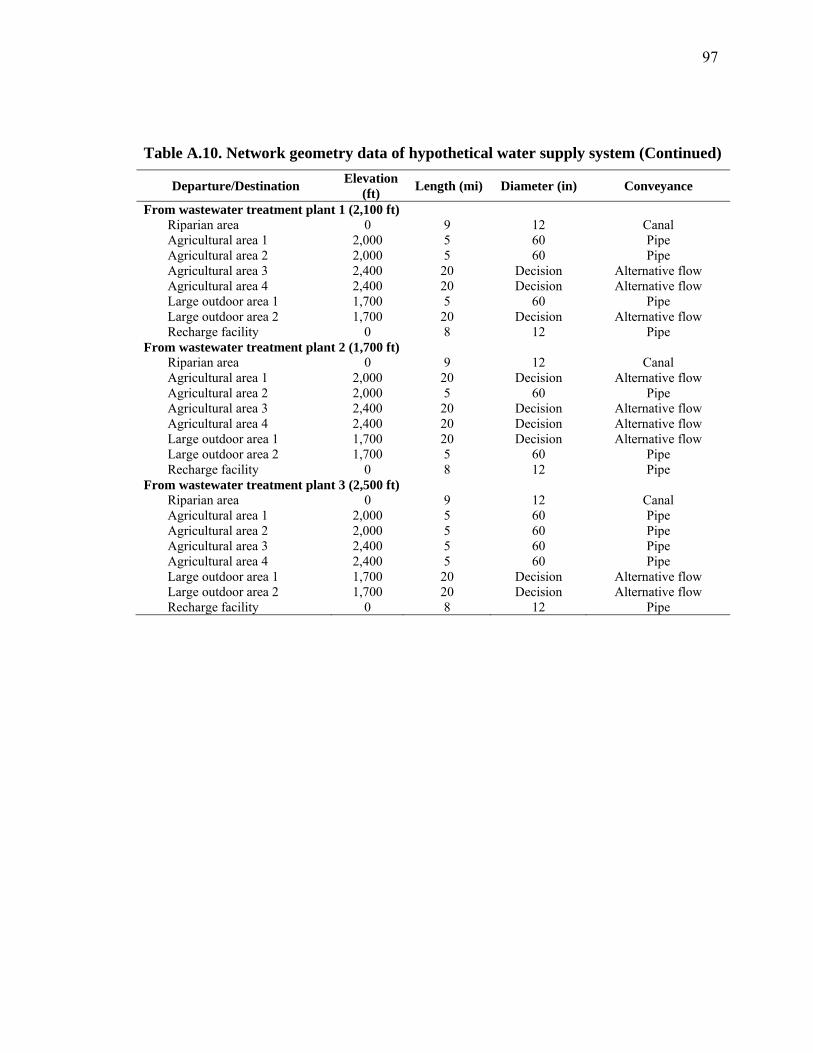
97
Table A.10. Network geometry data of hypothetical water supply system (Continued)
Departure/Destination Elevation (ft) Length (mi) Diameter (in) Conveyance
From wastewater treatment plant 1 (2,100 ft) Riparian area 0 9 12 Canal Agricultural area 1 2,000 5 60 Pipe Agricultural area 2 2,000 5 60 Pipe Agricultural area 3 2,400 20 Decision Alternative flow Agricultural area 4 2,400 20 Decision Alternative flow Large outdoor area 1 1,700 5 60 Pipe Large outdoor area 2 1,700 20 Decision Alternative flow Recharge facility 0 8 12 Pipe
From wastewater treatment plant 2 (1,700 ft) Riparian area 0 9 12 Canal Agricultural area 1 2,000 20 Decision Alternative flow Agricultural area 2 2,000 5 60 Pipe Agricultural area 3 2,400 20 Decision Alternative flow Agricultural area 4 2,400 20 Decision Alternative flow Large outdoor area 1 1,700 20 Decision Alternative flow Large outdoor area 2 1,700 5 60 Pipe Recharge facility 0 8 12 Pipe
From wastewater treatment plant 3 (2,500 ft) Riparian area 0 9 12 Canal Agricultural area 1 2,000 5 60 Pipe Agricultural area 2 2,000 5 60 Pipe Agricultural area 3 2,400 5 60 Pipe Agricultural area 4 2,400 5 60 Pipe Large outdoor area 1 1,700 20 Decision Alternative flow Large outdoor area 2 1,700 20 Decision Alternative flow Recharge facility 0 8 12 Pipe
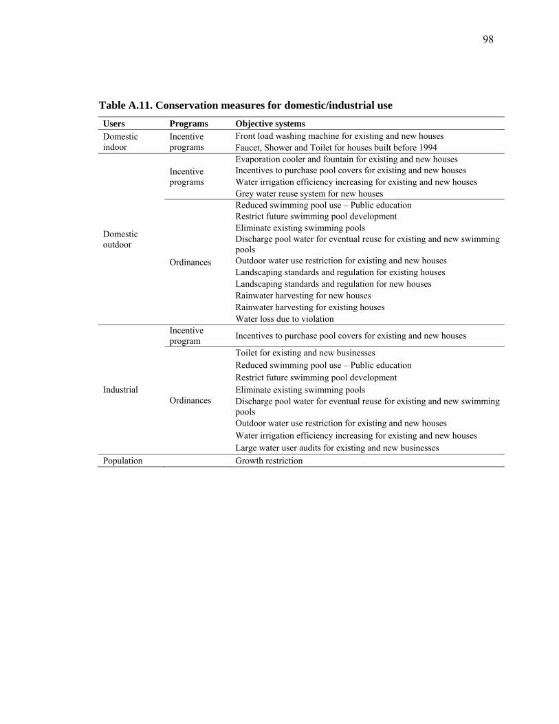
98
Table A.11. Conservation measures for domestic/industrial use Users Programs Objective systems Domestic indoor
Incentive programs
Front load washing machine for existing and new houses Faucet, Shower and Toilet for houses built before 1994
Domestic outdoor
Incentive programs
Evaporation cooler and fountain for existing and new houses Incentives to purchase pool covers for existing and new houses Water irrigation efficiency increasing for existing and new houses Grey water reuse system for new houses
Ordinances
Reduced swimming pool use – Public education Restrict future swimming pool development Eliminate existing swimming pools Discharge pool water for eventual reuse for existing and new swimming pools Outdoor water use restriction for existing and new houses Landscaping standards and regulation for existing houses Landscaping standards and regulation for new houses Rainwater harvesting for new houses Rainwater harvesting for existing houses Water loss due to violation
Industrial
Incentive program Incentives to purchase pool covers for existing and new houses
Ordinances
Toilet for existing and new businesses Reduced swimming pool use – Public education Restrict future swimming pool development Eliminate existing swimming pools Discharge pool water for eventual reuse for existing and new swimming pools Outdoor water use restriction for existing and new houses Water irrigation efficiency increasing for existing and new houses Large water user audits for existing and new businesses
Population Growth restriction
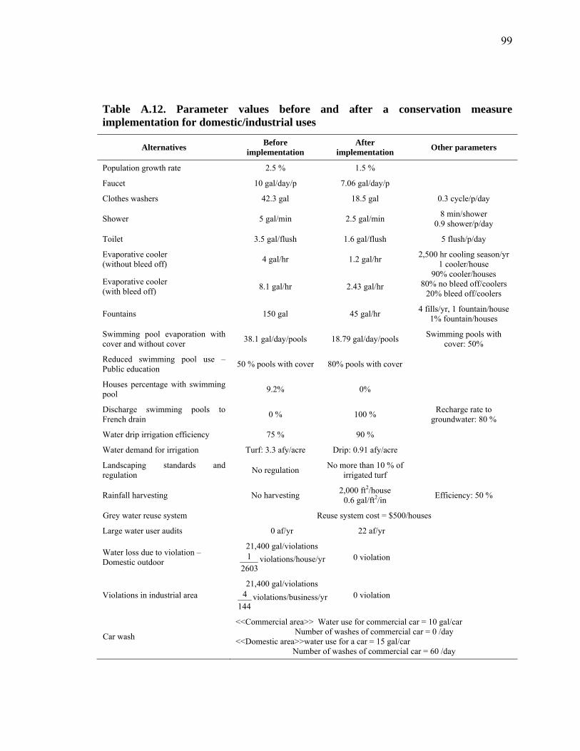
99
Table A.12. Parameter values before and after a conservation measure implementation for domestic/industrial uses
Alternatives Before implementation
After implementation Other parameters
Population growth rate 2.5 % 1.5 %
Faucet 10 gal/day/p 7.06 gal/day/p
Clothes washers 42.3 gal 18.5 gal 0.3 cycle/p/day
Shower 5 gal/min 2.5 gal/min 8 min/shower 0.9 shower/p/day
Toilet 3.5 gal/flush 1.6 gal/flush 5 flush/p/day
Evaporative cooler (without bleed off) 4 gal/hr 1.2 gal/hr 2,500 hr cooling season/yr
1 cooler/house 90% cooler/houses
80% no bleed off/coolers 20% bleed off/coolers
Evaporative cooler (with bleed off) 8.1 gal/hr 2.43 gal/hr
Fountains 150 gal 45 gal/hr 4 fills/yr, 1 fountain/house 1% fountain/houses
Swimming pool evaporation with cover and without cover 38.1 gal/day/pools 18.79 gal/day/pools Swimming pools with
cover: 50%
Reduced swimming pool use – Public education 50 % pools with cover 80% pools with cover
Houses percentage with swimming pool 9.2% 0%
Discharge swimming pools to French drain 0 % 100 % Recharge rate to
groundwater: 80 %
Water drip irrigation efficiency 75 % 90 %
Water demand for irrigation Turf: 3.3 afy/acre Drip: 0.91 afy/acre
Landscaping standards and regulation No regulation No more than 10 % of
irrigated turf
Rainfall harvesting No harvesting 2,000 ft2/house 0.6 gal/ft2/in Efficiency: 50 %
Grey water reuse system Reuse system cost = $500/houses
Large water user audits 0 af/yr 22 af/yr
Water loss due to violation – Domestic outdoor
21,400 gal/violations
26031 violations/house/yr 0 violation
Violations in industrial area 21,400 gal/violations
1444 violations/business/yr 0 violation
Car wash
<<Commercial area>> Water use for commercial car = 10 gal/car Number of washes of commercial car = 0 /day
<<Domestic area>>water use for a car = 15 gal/car Number of washes of commercial car = 60 /day
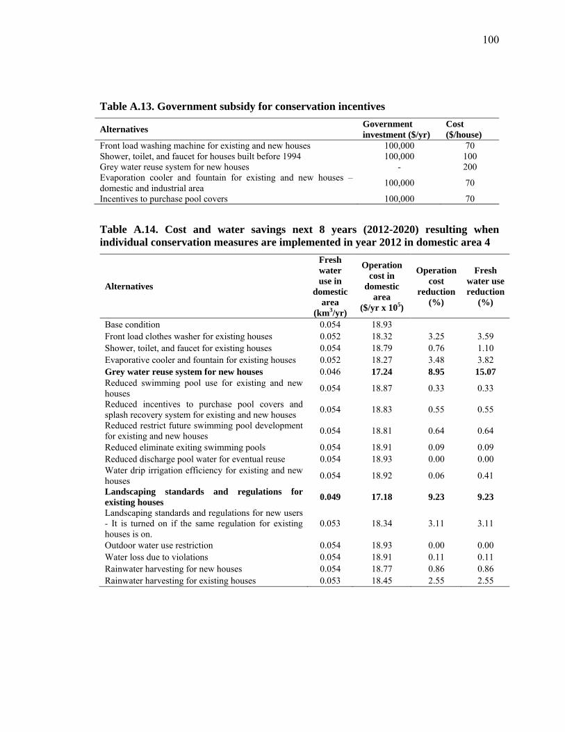
100
Table A.13. Government subsidy for conservation incentives
Alternatives Government investment ($/yr)
Cost ($/house)
Front load washing machine for existing and new houses 100,000 70 Shower, toilet, and faucet for houses built before 1994 100,000 100 Grey water reuse system for new houses - 200 Evaporation cooler and fountain for existing and new houses – domestic and industrial area 100,000 70
Incentives to purchase pool covers 100,000 70
Table A.14. Cost and water savings next 8 years (2012-2020) resulting when individual conservation measures are implemented in year 2012 in domestic area 4
Alternatives
Fresh water use in
domestic area
(km3/yr)
Operation cost in
domestic area
($/yr x 105)
Operation cost
reduction (%)
Fresh water use reduction
(%)
Base condition 0.054 18.93 Front load clothes washer for existing houses 0.052 18.32 3.25 3.59 Shower, toilet, and faucet for existing houses 0.054 18.79 0.76 1.10 Evaporative cooler and fountain for existing houses 0.052 18.27 3.48 3.82 Grey water reuse system for new houses 0.046 17.24 8.95 15.07 Reduced swimming pool use for existing and new houses 0.054 18.87 0.33 0.33
Reduced incentives to purchase pool covers and splash recovery system for existing and new houses 0.054 18.83 0.55 0.55
Reduced restrict future swimming pool development for existing and new houses 0.054 18.81 0.64 0.64
Reduced eliminate exiting swimming pools 0.054 18.91 0.09 0.09 Reduced discharge pool water for eventual reuse 0.054 18.93 0.00 0.00 Water drip irrigation efficiency for existing and new houses 0.054 18.92 0.06 0.41
Landscaping standards and regulations for existing houses 0.049 17.18 9.23 9.23
Landscaping standards and regulations for new users - It is turned on if the same regulation for existing houses is on.
0.053 18.34 3.11 3.11
Outdoor water use restriction 0.054 18.93 0.00 0.00 Water loss due to violations 0.054 18.91 0.11 0.11 Rainwater harvesting for new houses 0.054 18.77 0.86 0.86 Rainwater harvesting for existing houses 0.053 18.45 2.55 2.55
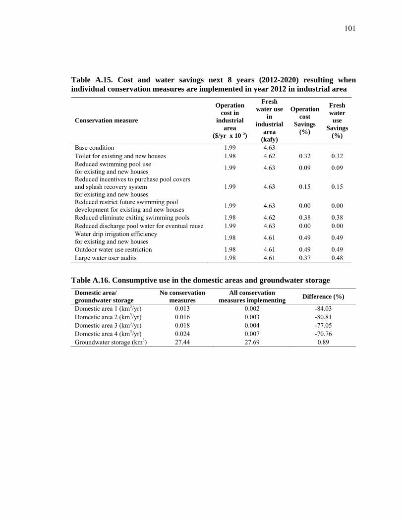
101
Table A.15. Cost and water savings next 8 years (2012-2020) resulting when individual conservation measures are implemented in year 2012 in industrial area
Conservation measure
Operation cost in
industrial area
($/yr x 10 5)
Fresh water use
in industrial
area (kafy)
Operation cost
Savings (%)
Fresh water
use Savings
(%)
Base condition 1.99 4.63 Toilet for existing and new houses 1.98 4.62 0.32 0.32 Reduced swimming pool use for existing and new houses 1.99 4.63 0.09 0.09
Reduced incentives to purchase pool covers and splash recovery system for existing and new houses
1.99 4.63 0.15 0.15
Reduced restrict future swimming pool development for existing and new houses 1.99 4.63 0.00 0.00
Reduced eliminate exiting swimming pools 1.98 4.62 0.38 0.38 Reduced discharge pool water for eventual reuse 1.99 4.63 0.00 0.00 Water drip irrigation efficiency for existing and new houses 1.98 4.61 0.49 0.49
Outdoor water use restriction 1.98 4.61 0.49 0.49 Large water user audits 1.98 4.61 0.37 0.48
Table A.16. Consumptive use in the domestic areas and groundwater storage Domestic area/ groundwater storage
No conservation measures
All conservation measures implementing Difference (%)
Domestic area 1 (km3/yr) 0.013 0.002 -84.03 Domestic area 2 (km3/yr) 0.016 0.003 -80.81 Domestic area 3 (km3/yr) 0.018 0.004 -77.05 Domestic area 4 (km3/yr) 0.024 0.007 -70.76 Groundwater storage (km3) 27.44 27.69 0.89
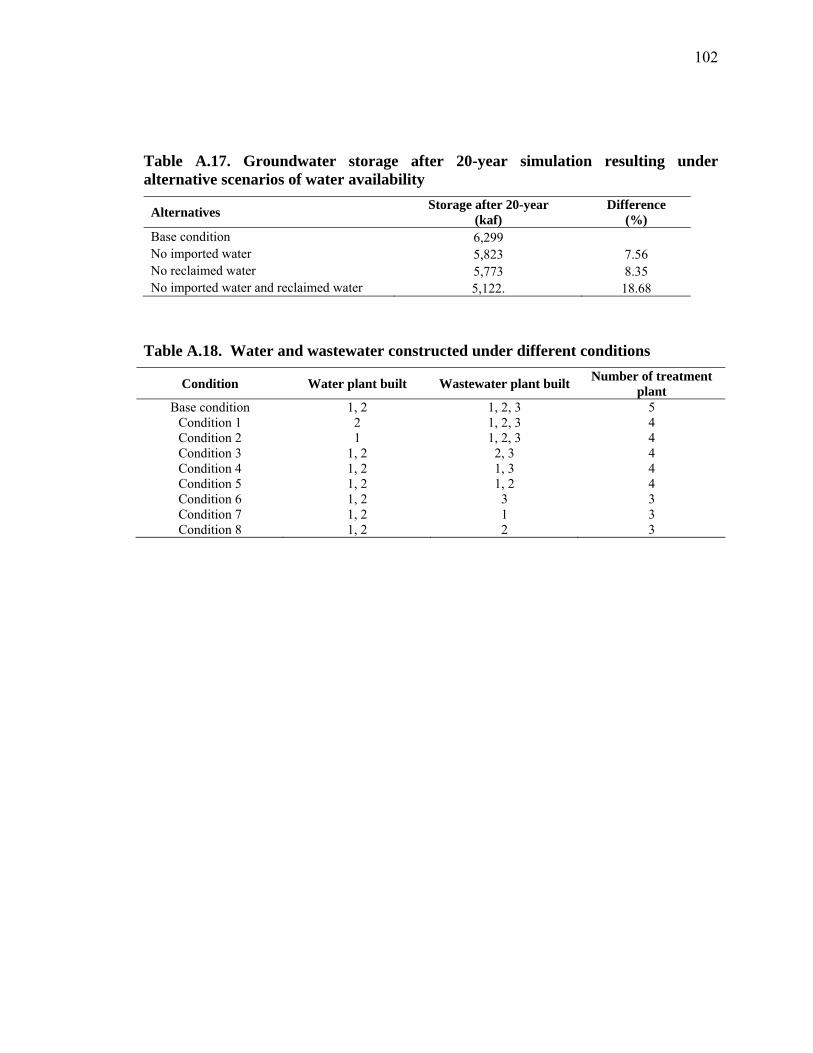
102
Table A.17. Groundwater storage after 20-year simulation resulting under alternative scenarios of water availability
Alternatives Storage after 20-year (kaf)
Difference (%)
Base condition 6,299 No imported water 5,823 7.56 No reclaimed water 5,773 8.35 No imported water and reclaimed water 5,122. 18.68
Table A.18. Water and wastewater constructed under different conditions
Condition Water plant built Wastewater plant built Number of treatment plant
Base condition 1, 2 1, 2, 3 5Condition 1 2 1, 2, 3 4Condition 2 1 1, 2, 3 4Condition 3 1, 2 2, 3 4Condition 4 1, 2 1, 3 4Condition 5 1, 2 1, 2 4Condition 6 1, 2 3 3Condition 7 1, 2 1 3Condition 8 1, 2 2 3
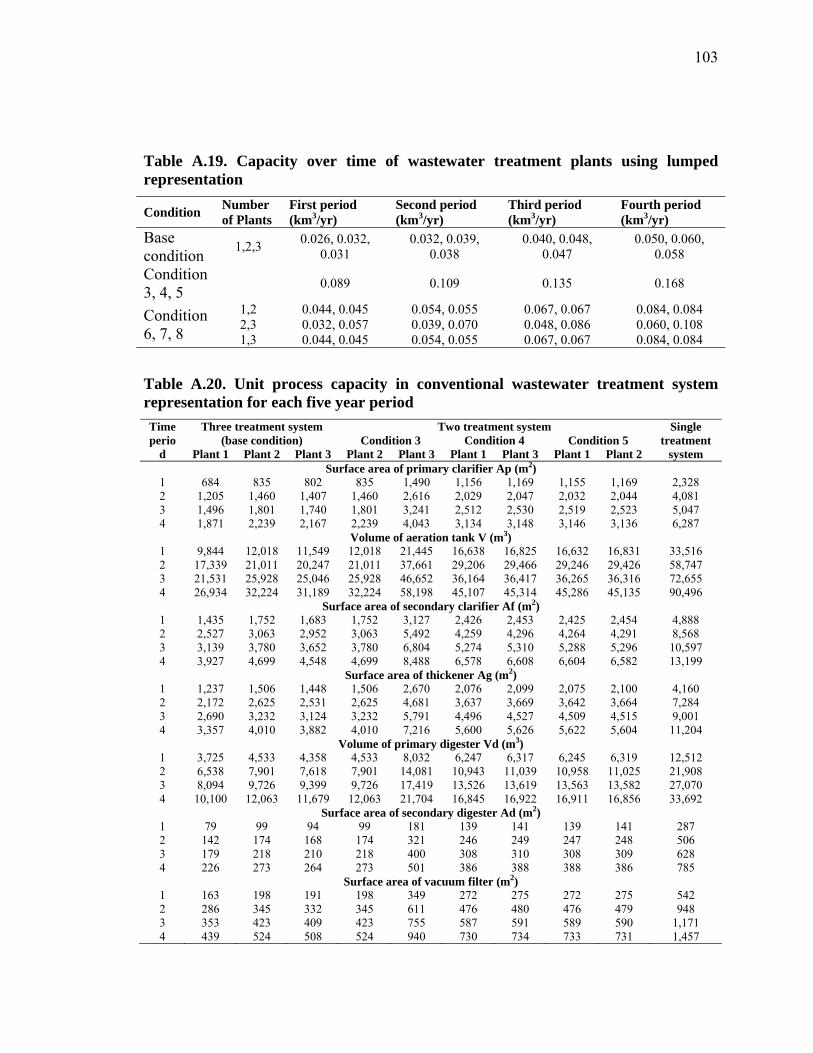
103
Table A.19. Capacity over time of wastewater treatment plants using lumped representation
Condition Number of Plants
First period (km3/yr)
Second period (km3/yr)
Third period (km3/yr)
Fourth period (km3/yr)
Base condition 1,2,3 0.026, 0.032,
0.031 0.032, 0.039,
0.038 0.040, 0.048,
0.047 0.050, 0.060,
0.058 Condition 3, 4, 5 0.089 0.109 0.135 0.168
Condition 6, 7, 8
1,2 0.044, 0.045 0.054, 0.055 0.067, 0.067 0.084, 0.084 2,3 0.032, 0.057 0.039, 0.070 0.048, 0.086 0.060, 0.108 1,3 0.044, 0.045 0.054, 0.055 0.067, 0.067 0.084, 0.084
Table A.20. Unit process capacity in conventional wastewater treatment system representation for each five year period Time perio
d
Three treatment system (base condition)
Two treatment system Single treatment
system Condition 3 Condition 4 Condition 5
Plant 1 Plant 2 Plant 3 Plant 2 Plant 3 Plant 1 Plant 3 Plant 1 Plant 2 Surface area of primary clarifier Ap (m2)
1 684 835 802 835 1,490 1,156 1,169 1,155 1,169 2,328 2 1,205 1,460 1,407 1,460 2,616 2,029 2,047 2,032 2,044 4,081 3 1,496 1,801 1,740 1,801 3,241 2,512 2,530 2,519 2,523 5,047 4 1,871 2,239 2,167 2,239 4,043 3,134 3,148 3,146 3,136 6,287
Volume of aeration tank V (m3) 1 9,844 12,018 11,549 12,018 21,445 16,638 16,825 16,632 16,831 33,516 2 17,339 21,011 20,247 21,011 37,661 29,206 29,466 29,246 29,426 58,747 3 21,531 25,928 25,046 25,928 46,652 36,164 36,417 36,265 36,316 72,655 4 26,934 32,224 31,189 32,224 58,198 45,107 45,314 45,286 45,135 90,496
Surface area of secondary clarifier Af (m2) 1 1,435 1,752 1,683 1,752 3,127 2,426 2,453 2,425 2,454 4,888 2 2,527 3,063 2,952 3,063 5,492 4,259 4,296 4,264 4,291 8,568 3 3,139 3,780 3,652 3,780 6,804 5,274 5,310 5,288 5,296 10,597 4 3,927 4,699 4,548 4,699 8,488 6,578 6,608 6,604 6,582 13,199
Surface area of thickener Ag (m2) 1 1,237 1,506 1,448 1,506 2,670 2,076 2,099 2,075 2,100 4,160 2 2,172 2,625 2,531 2,625 4,681 3,637 3,669 3,642 3,664 7,284 3 2,690 3,232 3,124 3,232 5,791 4,496 4,527 4,509 4,515 9,001 4 3,357 4,010 3,882 4,010 7,216 5,600 5,626 5,622 5,604 11,204
Volume of primary digester Vd (m3) 1 3,725 4,533 4,358 4,533 8,032 6,247 6,317 6,245 6,319 12,512 2 6,538 7,901 7,618 7,901 14,081 10,943 11,039 10,958 11,025 21,908 3 8,094 9,726 9,399 9,726 17,419 13,526 13,619 13,563 13,582 27,070 4 10,100 12,063 11,679 12,063 21,704 16,845 16,922 16,911 16,856 33,692
Surface area of secondary digester Ad (m2) 1 79 99 94 99 181 139 141 139 141 287 2 142 174 168 174 321 246 249 247 248 506 3 179 218 210 218 400 308 310 308 309 628 4 226 273 264 273 501 386 388 388 386 785
Surface area of vacuum filter (m2) 1 163 198 191 198 349 272 275 272 275 542 2 286 345 332 345 611 476 480 476 479 948 3 353 423 409 423 755 587 591 589 590 1,171 4 439 524 508 524 940 730 734 733 731 1,457
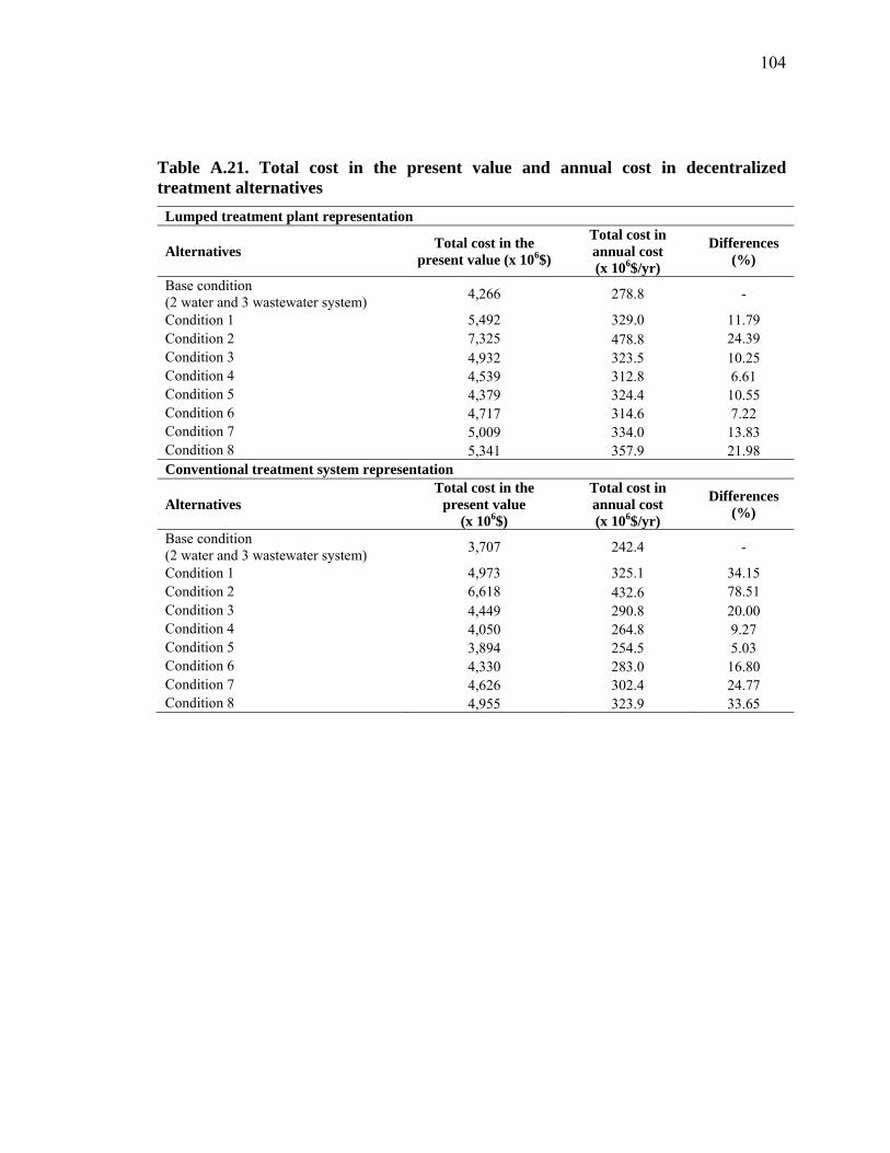
104
Table A.21. Total cost in the present value and annual cost in decentralized treatment alternatives
Lumped treatment plant representation
Alternatives Total cost in the present value (x 106$)
Total cost in annual cost (x 106$/yr)
Differences (%)
Base condition (2 water and 3 wastewater system) 4,266 278.8 -
Condition 1 5,492 329.0 11.79 Condition 2 7,325 478.8 24.39 Condition 3 4,932 323.5 10.25 Condition 4 4,539 312.8 6.61 Condition 5 4,379 324.4 10.55 Condition 6 4,717 314.6 7.22 Condition 7 5,009 334.0 13.83 Condition 8 5,341 357.9 21.98 Conventional treatment system representation
Alternatives Total cost in the
present value (x 106$)
Total cost in annual cost (x 106$/yr)
Differences (%)
Base condition (2 water and 3 wastewater system) 3,707 242.4 -
Condition 1 4,973 325.1 34.15 Condition 2 6,618 432.6 78.51 Condition 3 4,449 290.8 20.00 Condition 4 4,050 264.8 9.27 Condition 5 3,894 254.5 5.03 Condition 6 4,330 283.0 16.80 Condition 7 4,626 302.4 24.77 Condition 8 4,955 323.9 33.65
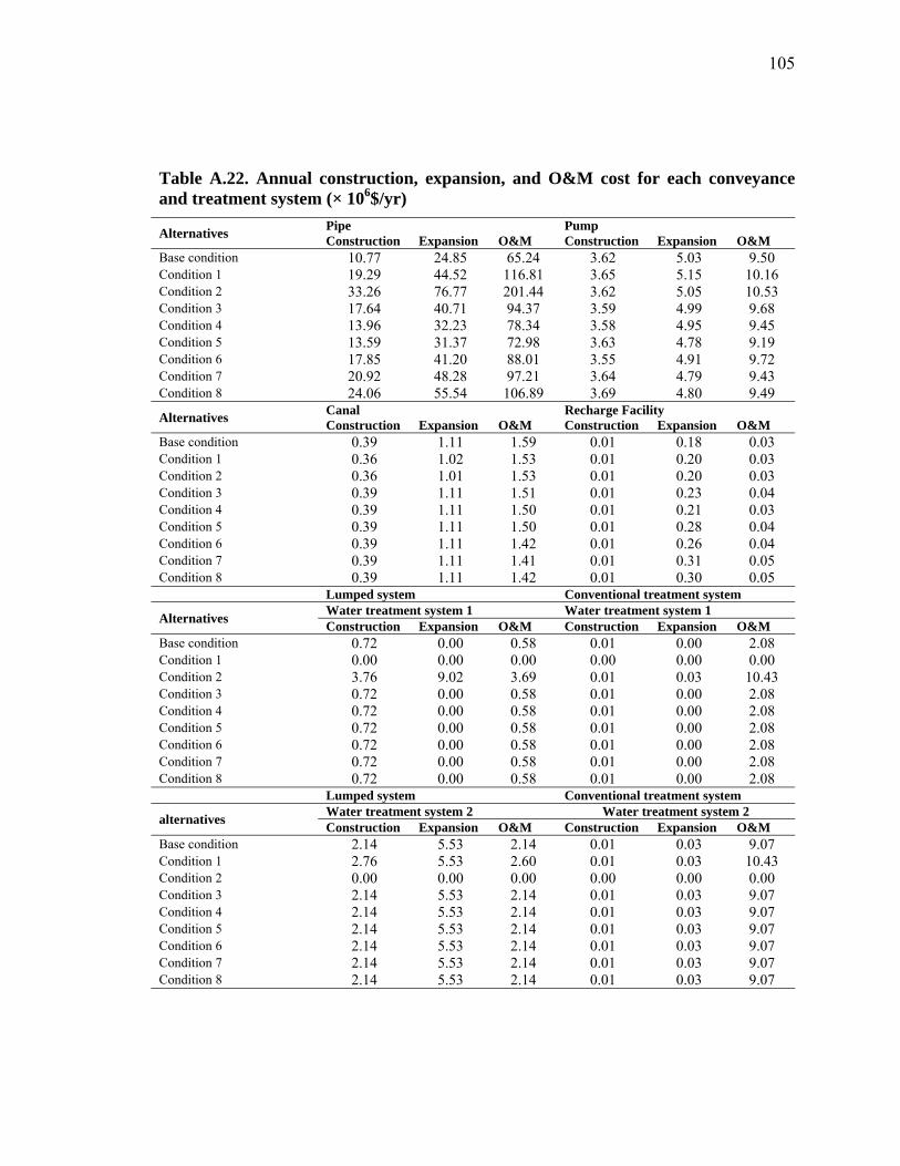
105
Table A.22. Annual construction, expansion, and O&M cost for each conveyance and treatment system (× 106$/yr)
Alternatives Pipe Pump Construction Expansion O&M Construction Expansion O&M
Base condition 10.77 24.85 65.24 3.62 5.03 9.50 Condition 1 19.29 44.52 116.81 3.65 5.15 10.16 Condition 2 33.26 76.77 201.44 3.62 5.05 10.53 Condition 3 17.64 40.71 94.37 3.59 4.99 9.68 Condition 4 13.96 32.23 78.34 3.58 4.95 9.45 Condition 5 13.59 31.37 72.98 3.63 4.78 9.19 Condition 6 17.85 41.20 88.01 3.55 4.91 9.72 Condition 7 20.92 48.28 97.21 3.64 4.79 9.43 Condition 8 24.06 55.54 106.89 3.69 4.80 9.49 Alternatives Canal Recharge Facility
Construction Expansion O&M Construction Expansion O&M Base condition 0.39 1.11 1.59 0.01 0.18 0.03 Condition 1 0.36 1.02 1.53 0.01 0.20 0.03 Condition 2 0.36 1.01 1.53 0.01 0.20 0.03 Condition 3 0.39 1.11 1.51 0.01 0.23 0.04 Condition 4 0.39 1.11 1.50 0.01 0.21 0.03 Condition 5 0.39 1.11 1.50 0.01 0.28 0.04 Condition 6 0.39 1.11 1.42 0.01 0.26 0.04 Condition 7 0.39 1.11 1.41 0.01 0.31 0.05 Condition 8 0.39 1.11 1.42 0.01 0.30 0.05 Lumped system Conventional treatment system
Alternatives Water treatment system 1 Water treatment system 1 Construction Expansion O&M Construction Expansion O&M
Base condition 0.72 0.00 0.58 0.01 0.00 2.08 Condition 1 0.00 0.00 0.00 0.00 0.00 0.00 Condition 2 3.76 9.02 3.69 0.01 0.03 10.43 Condition 3 0.72 0.00 0.58 0.01 0.00 2.08 Condition 4 0.72 0.00 0.58 0.01 0.00 2.08 Condition 5 0.72 0.00 0.58 0.01 0.00 2.08 Condition 6 0.72 0.00 0.58 0.01 0.00 2.08 Condition 7 0.72 0.00 0.58 0.01 0.00 2.08 Condition 8 0.72 0.00 0.58 0.01 0.00 2.08 Lumped system Conventional treatment system
alternatives Water treatment system 2 Water treatment system 2 Construction Expansion O&M Construction Expansion O&M
Base condition 2.14 5.53 2.14 0.01 0.03 9.07 Condition 1 2.76 5.53 2.60 0.01 0.03 10.43 Condition 2 0.00 0.00 0.00 0.00 0.00 0.00 Condition 3 2.14 5.53 2.14 0.01 0.03 9.07 Condition 4 2.14 5.53 2.14 0.01 0.03 9.07 Condition 5 2.14 5.53 2.14 0.01 0.03 9.07 Condition 6 2.14 5.53 2.14 0.01 0.03 9.07 Condition 7 2.14 5.53 2.14 0.01 0.03 9.07 Condition 8 2.14 5.53 2.14 0.01 0.03 9.07
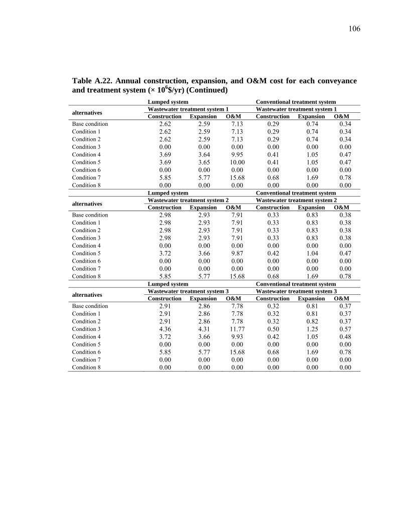
106
Table A.22. Annual construction, expansion, and O&M cost for each conveyance and treatment system (× 106$/yr) (Continued) Lumped system Conventional treatment system
alternatives Wastewater treatment system 1 Wastewater treatment system 1 Construction Expansion O&M Construction Expansion O&M
Base condition 2.62 2.59 7.13 0.29 0.74 0.34 Condition 1 2.62 2.59 7.13 0.29 0.74 0.34 Condition 2 2.62 2.59 7.13 0.29 0.74 0.34 Condition 3 0.00 0.00 0.00 0.00 0.00 0.00 Condition 4 3.69 3.64 9.95 0.41 1.05 0.47 Condition 5 3.69 3.65 10.00 0.41 1.05 0.47 Condition 6 0.00 0.00 0.00 0.00 0.00 0.00 Condition 7 5.85 5.77 15.68 0.68 1.69 0.78 Condition 8 0.00 0.00 0.00 0.00 0.00 0.00 Lumped system Conventional treatment system
alternatives Wastewater treatment system 2 Wastewater treatment system 2 Construction Expansion O&M Construction Expansion O&M
Base condition 2.98 2.93 7.91 0.33 0.83 0.38 Condition 1 2.98 2.93 7.91 0.33 0.83 0.38 Condition 2 2.98 2.93 7.91 0.33 0.83 0.38 Condition 3 2.98 2.93 7.91 0.33 0.83 0.38 Condition 4 0.00 0.00 0.00 0.00 0.00 0.00 Condition 5 3.72 3.66 9.87 0.42 1.04 0.47 Condition 6 0.00 0.00 0.00 0.00 0.00 0.00 Condition 7 0.00 0.00 0.00 0.00 0.00 0.00 Condition 8 5.85 5.77 15.68 0.68 1.69 0.78 Lumped system Conventional treatment system
alternatives Wastewater treatment system 3 Wastewater treatment system 3 Construction Expansion O&M Construction Expansion O&M
Base condition 2.91 2.86 7.78 0.32 0.81 0.37 Condition 1 2.91 2.86 7.78 0.32 0.81 0.37 Condition 2 2.91 2.86 7.78 0.32 0.82 0.37 Condition 3 4.36 4.31 11.77 0.50 1.25 0.57 Condition 4 3.72 3.66 9.93 0.42 1.05 0.48 Condition 5 0.00 0.00 0.00 0.00 0.00 0.00 Condition 6 5.85 5.77 15.68 0.68 1.69 0.78 Condition 7 0.00 0.00 0.00 0.00 0.00 0.00 Condition 8 0.00 0.00 0.00 0.00 0.00 0.00
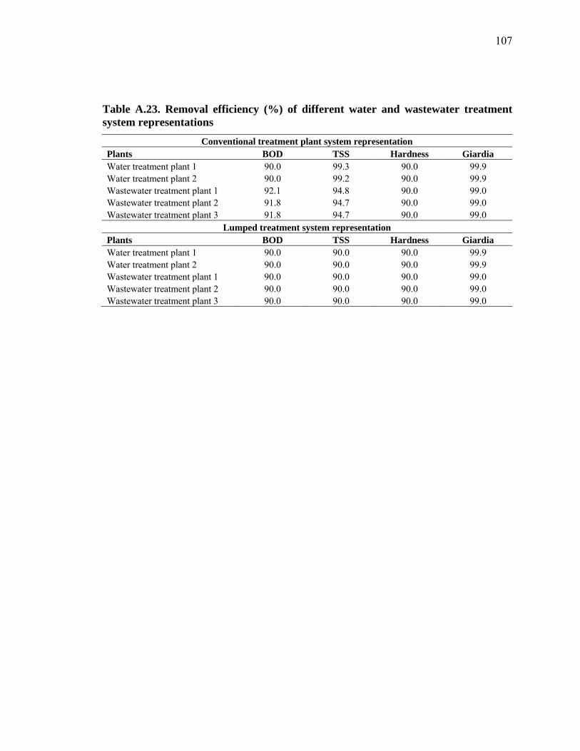
107
Table A.23. Removal efficiency (%) of different water and wastewater treatment system representations
Conventional treatment plant system representation Plants BOD TSS Hardness Giardia Water treatment plant 1 90.0 99.3 90.0 99.9 Water treatment plant 2 90.0 99.2 90.0 99.9 Wastewater treatment plant 1 92.1 94.8 90.0 99.0 Wastewater treatment plant 2 91.8 94.7 90.0 99.0 Wastewater treatment plant 3 91.8 94.7 90.0 99.0
Lumped treatment system representation Plants BOD TSS Hardness Giardia Water treatment plant 1 90.0 90.0 90.0 99.9 Water treatment plant 2 90.0 90.0 90.0 99.9 Wastewater treatment plant 1 90.0 90.0 90.0 99.0 Wastewater treatment plant 2 90.0 90.0 90.0 99.0 Wastewater treatment plant 3 90.0 90.0 90.0 99.0
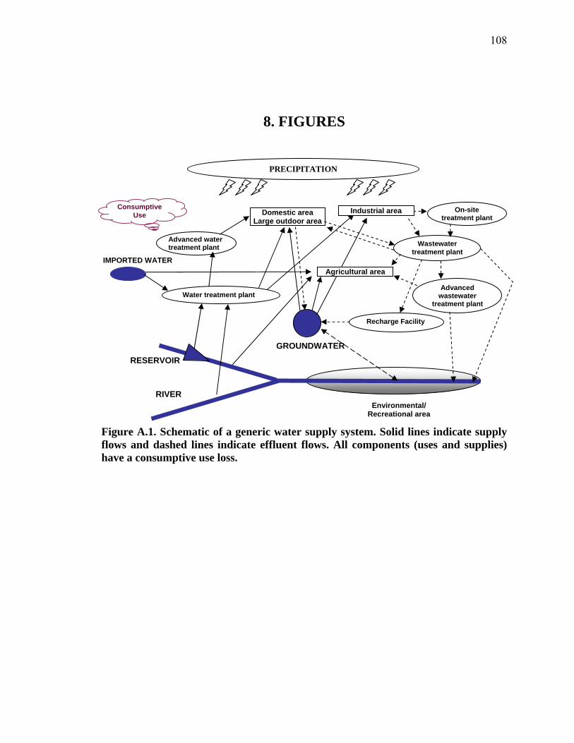
108
8. FIGURES
Figure A.1. Schematic of a generic water supply system. Solid lines indicate supply flows and dashed lines indicate effluent flows. All components (uses and supplies) have a consumptive use loss.
PRECIPITATION
IMPORTED WATER
Environmental/ Recreational area
Domestic area Large outdoor area
Water treatment plant
Advanced water treatment plant Wastewater
treatment plant
Advancedwastewater
treatment plant
Recharge Facility
GROUNDWATER
RIVER
RESERVOIR
On-site treatment plant
Consumptive Use
Agricultural area
Industrial area
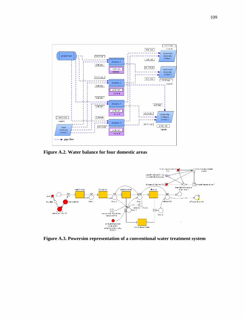
109
Figure A.2. Water balance for four domestic areas
Figure A.3. Powersim representation of a conventional water treatment system
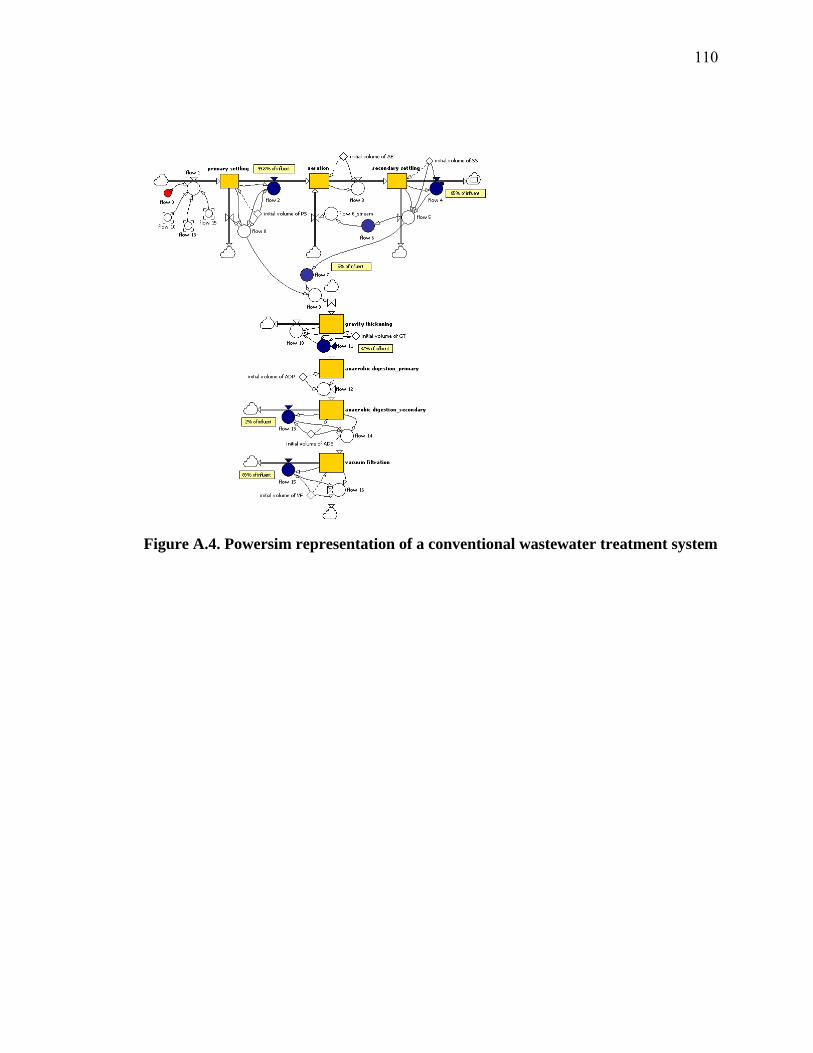
110
Figure A.4. Powersim representation of a conventional wastewater treatment system
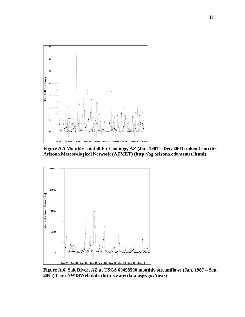
111
Jan-87 Jan-89 Jan-91 Jan-93 Jan-95 Jan-97 Jan-99 Jan-01 Jan-03 Jan-05
0
1
2
3
4
5
6
7R
ainf
all (
inch
es)
Figure A.5 Monthly rainfall for Coolidge, AZ (Jan. 1987 – Dec. 2004) taken from the Arizona Meteorological Network (AZMET) (http://ag.arizona.edu/azmet/.html)
Jan-87 Jan-89 Jan-91 Jan-93 Jan-95 Jan-97 Jan-99 Jan-01 Jan-03
0
4000
8000
12000
16000
Nat
ural
str
eam
flow
(cfs
)
Figure A.6. Salt River, AZ at USGS 09498500 monthly streamflows (Jan. 1987 – Sep. 2004) from NWISWeb data (http://waterdata.usgs.gov/nwis)
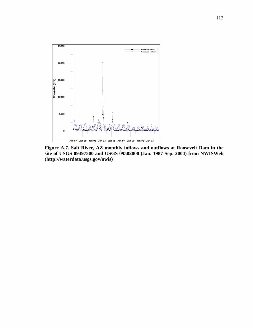
112
Jan-87 Jan-89 Jan-91 Jan-93 Jan-95 Jan-97 Jan-99 Jan-01 Jan-03
0
5000
10000
15000
20000
25000
flow
rate
(cfs
)Reservoir inflowReservoir outflow
Figure A.7. Salt River, AZ monthly inflows and outflows at Roosevelt Dam in the site of USGS 09497500 and USGS 09502000 (Jan. 1987-Sep. 2004) from NWISWeb (http://waterdata.usgs.gov/nwis)
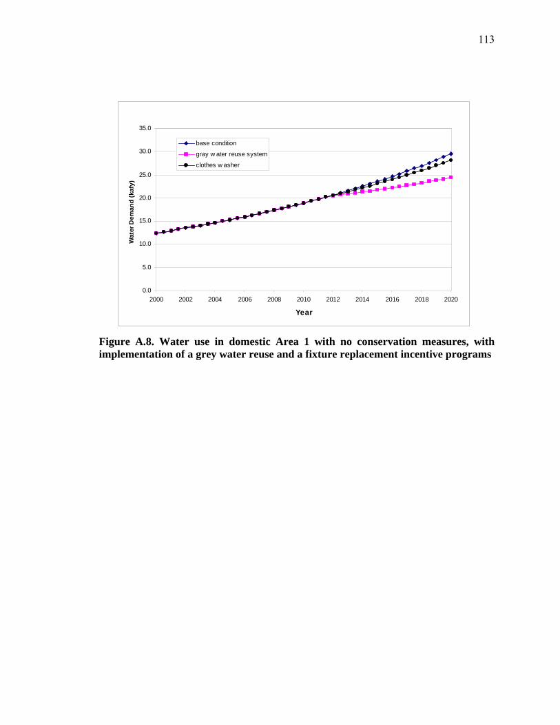
113
0.0
5.0
10.0
15.0
20.0
25.0
30.0
35.0
2000 2002 2004 2006 2008 2010 2012 2014 2016 2018 2020
Year
Wat
er D
eman
d (k
afy)
base condition
gray w ater reuse system
clothes w asher
Figure A.8. Water use in domestic Area 1 with no conservation measures, with implementation of a grey water reuse and a fixture replacement incentive programs
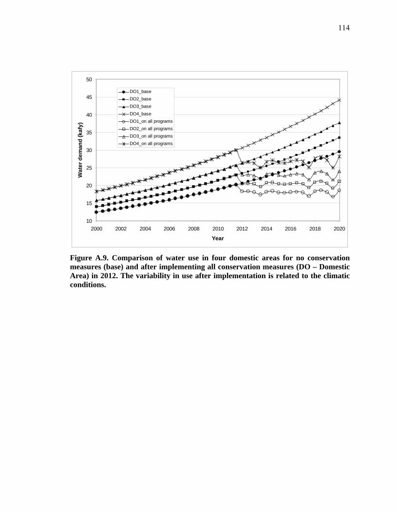
114
10
15
20
25
30
35
40
45
50
2000 2002 2004 2006 2008 2010 2012 2014 2016 2018 2020
Year
Wat
er d
eman
d (k
afy)
DO1_baseDO2_baseDO3_baseDO4_baseDO1_on all programsDO2_on all programsDO3_on all programsDO4_on all programs
Figure A.9. Comparison of water use in four domestic areas for no conservation measures (base) and after implementing all conservation measures (DO – Domestic Area) in 2012. The variability in use after implementation is related to the climatic conditions.

115
0.0E+00
5.0E+08
1.0E+09
1.5E+09
2.0E+09
2.5E+09
3.0E+09
3.5E+09
4.0E+09
2000 2002 2004 2006 2008 2010 2012 2014 2016 2018 2020
Year
Tota
l cos
t ($)
Base conditionConservation measures
Figure A.10. Cost for constructing and operating entire system over time for no conservation measures (base) and after implementing all conservation measures in year 2012
Figure A.11. Inflows from various sources to agricultural area 1 during growing season for meeting consumptive use with reclaimed water and imported water
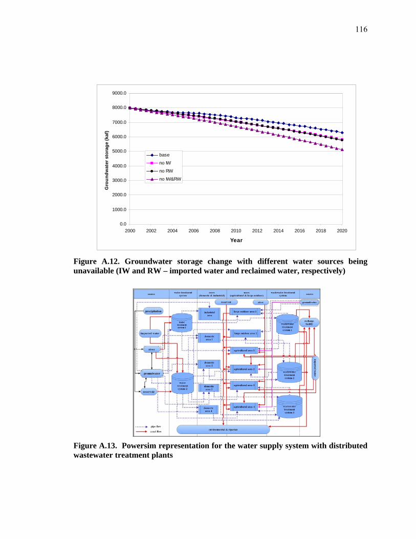
116
0.0
1000.0
2000.0
3000.0
4000.0
5000.0
6000.0
7000.0
8000.0
9000.0
2000 2002 2004 2006 2008 2010 2012 2014 2016 2018 2020
Year
Gro
undw
ater
sto
rage
(kaf
)
base
no IW
no RW
no IW&RW
Figure A.12. Groundwater storage change with different water sources being unavailable (IW and RW – imported water and reclaimed water, respectively)
Figure A.13. Powersim representation for the water supply system with distributed wastewater treatment plants
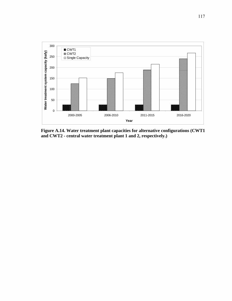
117
0
50
100
150
200
250
300
2000-2005 2006-2010 2011-2015 2016-2020
Year
Wat
er tr
eatm
ent s
yste
m c
apac
ity (k
afy)
CWT1CWT2Single Capacity
Figure A.14. Water treatment plant capacities for alternative configurations (CWT1 and CWT2 - central water treatment plant 1 and 2, respectively.)
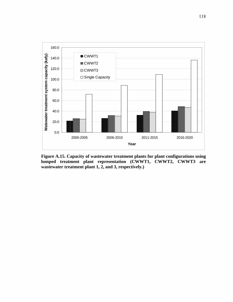
118
0.0
20.0
40.0
60.0
80.0
100.0
120.0
140.0
160.0
2000-2005 2006-2010 2011-2015 2016-2020
Year
Wat
ewat
er tr
eatm
ent s
yste
m c
apac
ity (k
afy) CWWT1
CWWT2
CWWT3
Single Capacity
Figure A.15. Capacity of wastewater treatment plants for plant configurations using lumped treatment plant representation (CWWT1, CWWT2, CWWT3 are wastewater treatment plant 1, 2, and 3, respectively.)
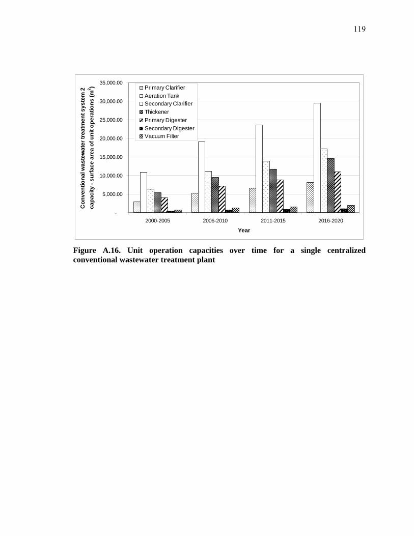
119
-
5,000.00
10,000.00
15,000.00
20,000.00
25,000.00
30,000.00
35,000.00
2000-2005 2006-2010 2011-2015 2016-2020
Year
Con
vent
iona
l was
tew
ater
trea
tmen
t sys
tem
2
capa
city
- su
rface
are
a of
uni
t ope
ratio
ns (m
2 ) Primary ClarifierAeration TankSecondary ClarifierThickenerPrimary DigesterSecondary DigesterVacuum Filter
Figure A.16. Unit operation capacities over time for a single centralized conventional wastewater treatment plant
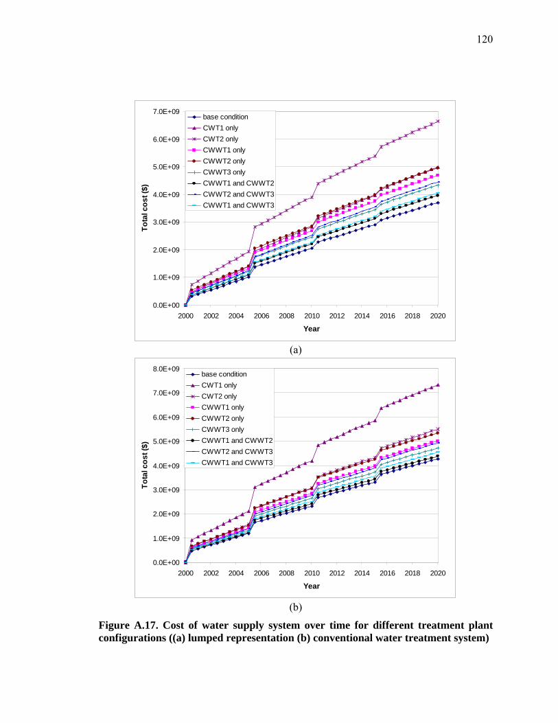
120
0.0E+00
1.0E+09
2.0E+09
3.0E+09
4.0E+09
5.0E+09
6.0E+09
7.0E+09
2000 2002 2004 2006 2008 2010 2012 2014 2016 2018 2020
Year
Tota
l cos
t ($)
base conditionCWT1 onlyCWT2 onlyCWWT1 onlyCWWT2 onlyCWWT3 onlyCWWT1 and CWWT2CWWT2 and CWWT3CWWT1 and CWWT3
(a)
0.0E+00
1.0E+09
2.0E+09
3.0E+09
4.0E+09
5.0E+09
6.0E+09
7.0E+09
8.0E+09
2000 2002 2004 2006 2008 2010 2012 2014 2016 2018 2020
Year
Tota
l cos
t ($)
base conditionCWT1 onlyCWT2 onlyCWWT1 onlyCWWT2 onlyCWWT3 onlyCWWT1 and CWWT2CWWT2 and CWWT3CWWT1 and CWWT3
(b)
Figure A.17. Cost of water supply system over time for different treatment plant configurations ((a) lumped representation (b) conventional water treatment system)
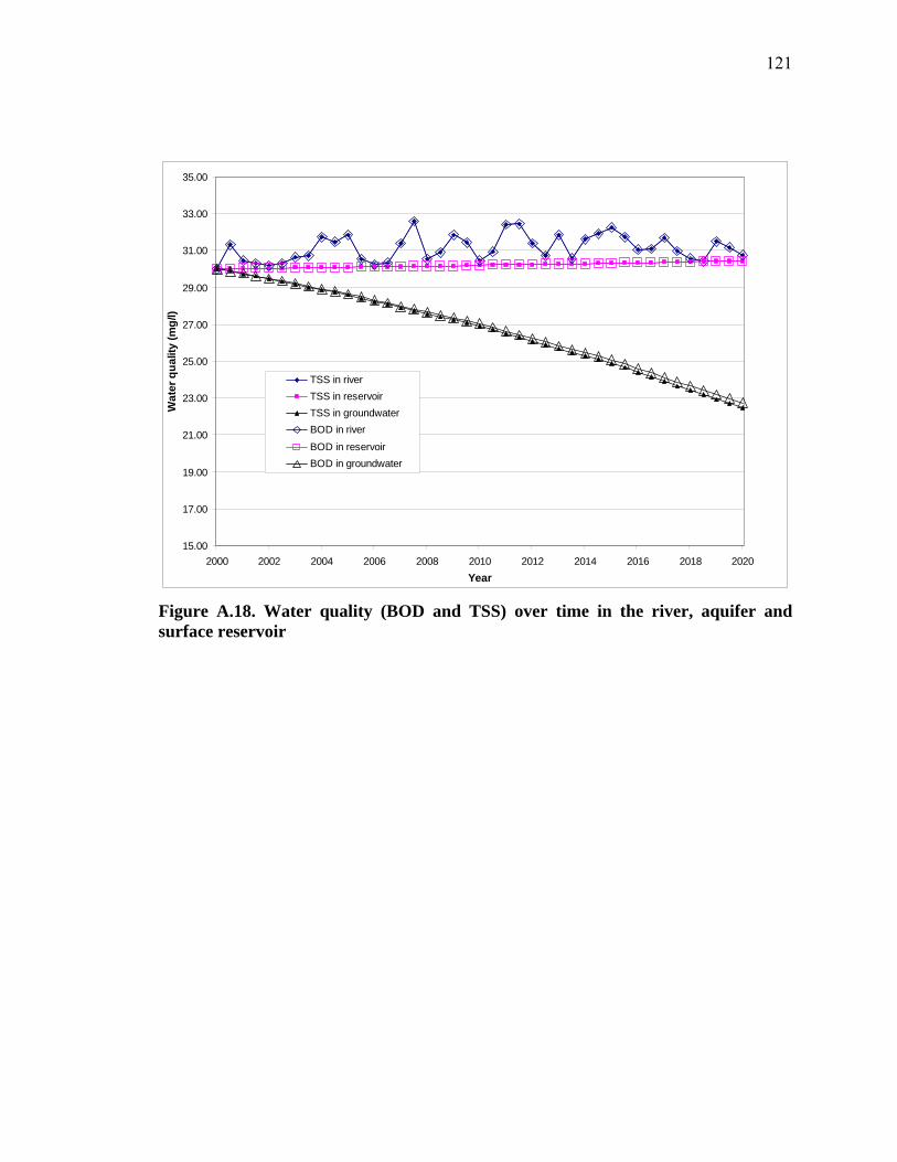
121
15.00
17.00
19.00
21.00
23.00
25.00
27.00
29.00
31.00
33.00
35.00
2000 2002 2004 2006 2008 2010 2012 2014 2016 2018 2020Year
Wat
er q
ualit
y (m
g/l)
TSS in riverTSS in reservoirTSS in groundwaterBOD in riverBOD in reservoirBOD in groundwater
Figure A.18. Water quality (BOD and TSS) over time in the river, aquifer and surface reservoir
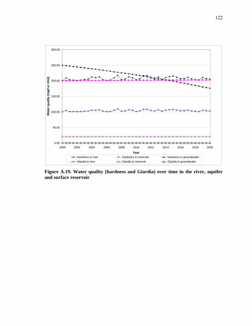
122
0.00
50.00
100.00
150.00
200.00
250.00
300.00
2000 2002 2004 2006 2008 2010 2012 2014 2016 2018 2020
Year
Wat
er q
ualit
y (m
g/l o
r #/m
l)
hardness in river hardness in reservoir hardness in groundwaterGiardia in river Giardia in reservoir Giardia in groundwater
Figure A.19. Water quality (hardness and Giardia) over time in the river, aquifer and surface reservoir
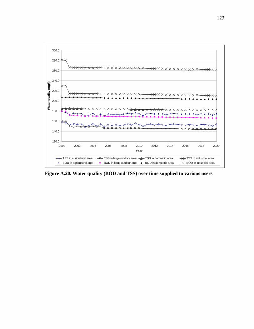
123
120.0
140.0
160.0
180.0
200.0
220.0
240.0
260.0
280.0
300.0
2000 2002 2004 2006 2008 2010 2012 2014 2016 2018 2020
Year
Wat
er q
ualit
y (m
g/l)
TSS in agricultural area TSS in large outdoor area TSS in domestic area TSS in industrial areaBOD in agricultural area BOD in large outdoor area BOD in domestic area BOD in industrial area
Figure A.20. Water quality (BOD and TSS) over time supplied to various users
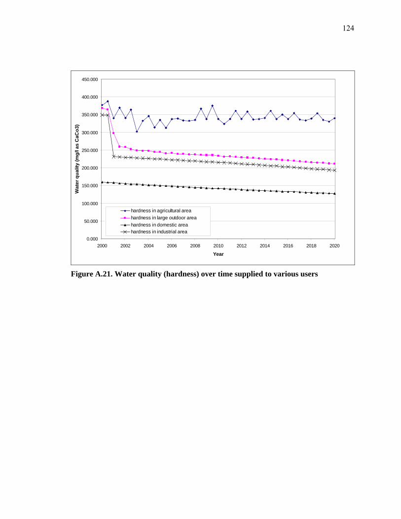
124
0.000
50.000
100.000
150.000
200.000
250.000
300.000
350.000
400.000
450.000
2000 2002 2004 2006 2008 2010 2012 2014 2016 2018 2020
Year
Wat
er q
ualit
y (m
g/l a
s C
aCo3
)
hardness in agricultural areahardness in large outdoor areahardness in domestic areahardness in industrial area
Figure A.21. Water quality (hardness) over time supplied to various users
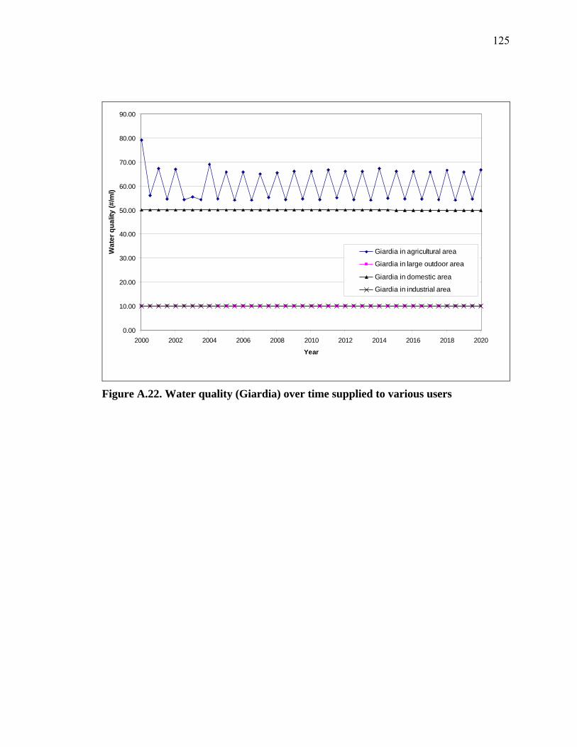
125
0.00
10.00
20.00
30.00
40.00
50.00
60.00
70.00
80.00
90.00
2000 2002 2004 2006 2008 2010 2012 2014 2016 2018 2020
Year
Wat
er q
ualit
y (#
/ml)
Giardia in agricultural area
Giardia in large outdoor area
Giardia in domestic area
Giardia in industrial area
Figure A.22. Water quality (Giardia) over time supplied to various users
126
APPENDIX B. APPLICATION OF THE SHUFFLED FROG
LEAPING ALGORITHM FOR THE OPTIMIZATION OF A
GENERAL LARGE-SCALE WATER SUPPLY SYSTEM
B. Graph
127
Application of the Shuffled Frog Leaping Algorithm for the Optimization
of a General Large-Scale Water Supply System
G. Chung1 and K. Lansey2
ABSTRACT
A water supply system is a complicated network of pipes, canals and storage and
treatment facilities that collects, treats, stores, and distributes water to consumers.
Increasing population and its associated demands requires systems to be expanded and
adapted over time to provide a sustainable water supply. Comprehensive design tools are
needed to assist managers determine how to plan for future growth. In this study, a
general large-scale water supply system model was developed to minimize the total
system cost by integrating a mathematical supply system representation and applying the
shuffled frog leaping algorithm optimization scheme (SFLA).
The developed model was applied to two hypothetical water communities. The
capacities for the system components including water transport and treatment facilities
are model decision variables. An explicit representation of energy consumption cost for
the transporting water in the model assists in determining the efficacy of satellite
wastewater treatment facilities.
1 Graduate Student, Department of Civil Engineering and Engineering Mechanics, The University of Arizona, Tucson, AZ 85721, USA (Tel: 1-520-360-9554, E-mail: [email protected]) 2 Professor, Department of Civil Engineering and Engineering Mechanics, The University of Arizona, Tucson, AZ 85721, USA (Tel: 1-520-621-2512, Fax: 1-520-621-2550, E-mail: [email protected])

128
Although the water supply systems studied contained highly nonlinear terms in the
formulation as well as several hundred decisions variables, the stochastic search
algorithm, SFLA, successfully found solutions that satisfied all the constraints for the
studied networks.
129
1. INTRODUCTION AND BACKGROUND
A water supply system is a collection of water transport structures, pumping stations,
and water treatment and storage facilities that are managed to supply the desired amount
of water with the desired quality to consumers. With increasing water demand from
domestic and industrial areas, sustainable water supply becomes more important and the
development of a long-term water supply plan is challenging because of complexity of
the system and uncertainties in the future.
In the southwest Unites States and many arid and semi-arid regions, groundwater is a
major water source but, oftentimes, it has been mined to meet the increased water
demands. As a result, ground water table level have fallen requiring better management
plans or identifying alternative water sources. Reclaimed and imported water are
potential alternatives that may replace groundwater for agricultural and other purposes. In
the future as new supplies become more limited, water reclaimed, after a high level of
treatment, may be necessary to meet potable demands.
Water supply planning requires considering current demand, future growth, and
available supplies. Supply costs include capital for construction, operation and
maintenance. As reclaimed water becomes a more integral part of the water supply
system, the cost of transporting water from a treatment facility to users becomes more
critical in decision making. This introduces another complexity to the planning process in
that the cost of distribution may exceed the gains in economies of scale that are obtained
130
if wastewater treatment is centralized. Hence, smaller distributed wastewater treatment
facilities may be a cost effective alternative over a single central plant.
Little research has been conducted on water supply system planning optimization.
Ocanas and Mays (1981a and b) formulated and solved a water reuse planning
optimization model using non-linear programming under steady and dynamic conditions.
The steady state model consisted of a nonlinear objective function, linear and nonlinear
constraints for a single period. A large-scale generalized reduced gradient technique was
used to solve this optimization problem (Ocanas and Mays 1981a). In the follow-up
paper, the same technique with successive linear programming methods was applied to a
dynamic water reuse planning model with single and multiple periods (Ocanas and Mays
1981b). Water quality was considered in both papers. In the dynamic model, the capacity
expansion of treatment facilities was considered at the beginning of the period and
operation costs were included in the objective function. This model provided a basis of
the optimization structure for a water supply management system. Conveyance systems
were considered as lumped units without detailed representations of energy loss and
capacity. Later, Ejeta et al. (2004) applied a general approach to the studies in Rio
Grande in New Mexico and Texas including a total suspended solids (TSS) constraint.
The objective of this study was to maximize total net benefit.
In this paper, the water reuse planning system formulated by Ocanas and Mays
(1981a and b) is extended to consider component hydraulic capacities and improve
scalability. Decision variables include the capacities of water transport facilities - such as
pipes, pumps, and canals - as well as the capacity of treatment facilities. This step extends
131
previous work in this area by optimizing overall system costs with an explicit
representation of energy consumption costs and evaluating the tradeoff of multiple
satellite wastewater treatment facilities. The problem considered in this study is highly
nonlinear and deals with a large-scale water supply system that involves several hundred
decisions. A stochastic search algorithm is successfully applied to determine the optimal
water supply plans for two hypothetical communities.
2. PROBLEM DESCRIPTION
The overall planning goal is to minimize the total costs of construction, operation and
maintenance of the water supply system. The problem considered in this paper extends
earlier work by considering operations costs as a function of flow rates and selected
component sizes. The supply system may have multiple sources and users, and contain
one or more water and wastewater treatment facilities. Unlike previous models,
conveyance system hydraulics are directly embedded in the model to more realistically
estimate operation expenses. One or more planning periods can be represented to allow
delaying expansion investments or to take advantage of economies of scale by
constructing excess capacity in early decision periods.
Figures B.1 and B.2 show system schematics for two communities. Potential flow
paths are shown between sources, sinks and users that are denoted as nodes. Water uses
are agricultural, domestic, industrial and large outdoor irrigation (golf courses, school,
and parks). Available water supply sources can include surface reservoirs or groundwater
132
aquifers that have storage capabilities and rivers that cannot store water over time. Any
flow provided to domestic and industrial users from surface water sources must be treated
at a water treatment facility (WT) while surface water provided to agricultural and
outdoor uses does not need to be treated. Wastewater return flows from domestic and
industrial uses must be treated at a wastewater treatment plant (WW). After wastewater
treatment, reclaimed water may be supplied to agricultural or large irrigation areas,
discharged to the river, or recharged to the aquifer through infiltration basins.
Groundwater banking can also be achieved by recharging imported waters or surface
supplies.
The primary system constraints are to satisfy conservation of mass at all locations and
components in the system. In addition, each user has defined water quality and demand
requirements, while all supplies are limited by flow capacity or storage volume.
Conveyance system conditions related to canal capacity and pipeline/pump sizes are
formulated to ensure proper sizing and energy consumption. The mathematical form of
the problem is given in the next section.
3. PROBLEM FORMULATION
A general system can be represented by a set of N nodes and A arcs. Arcs denote
water transmission systems while nodes are locations where water is collected from or
split between a set of arcs. The set of nodes is comprised of several subsets representing
sources (IS) and users (IR). Sources are further divided into storage sources (ISS) that
133
have storage carried over in time (groundwater aquifers and surface reservoirs) and non-
storage sources (INS) that cannot store water over time (rivers and imported waters (IIW)).
Note that a river is represented as upstream (IRU) and downstream nodes (IRD) that are
connected by a river arc. Water is withdrawn by users from upstream nodes and returned
from treatment plants to the downstream river. Water user nodes represent domestic,
industrial, and irrigational purposes and water and wastewater treatment plants (IWT, and
IWWT, respectively).
An arc transmits flow from a node i to a node j. Arcs represent the sets of canals (IC),
pipe connections (IP), pump connections (IU). Pipe connections may have pump stations
at their upstream source depending on the elevation difference and energy losses between
the two connected nodes. Recharge basin arcs (IB) can be used to transmit imported or
treated water to the aquifer to bank or recharge water in the aquifer. In addition, rivers
and users may recharge the aquifer through seepage or infiltration that is represented by
infiltration arcs (II).
The capacities of the water transmission structures such as pipes, pumps, and canals
and treatment plants are described as structural variables. Flow allocations over the water
supply network are operational variables.
The objective function consists of the function of construction and expansion, and
operations and maintenance (O&M) costs for all components (pipes, canals, pumps, and
treatment facilities) or:
654321* ),()(),()()(Minimize fwqfwfHfffZ t
itij
ti
tij
tij
tij
tij +++++= χκκ (B.1)
Each term in Eq. B.1 is non-linear relationship with respect to the decision variables.
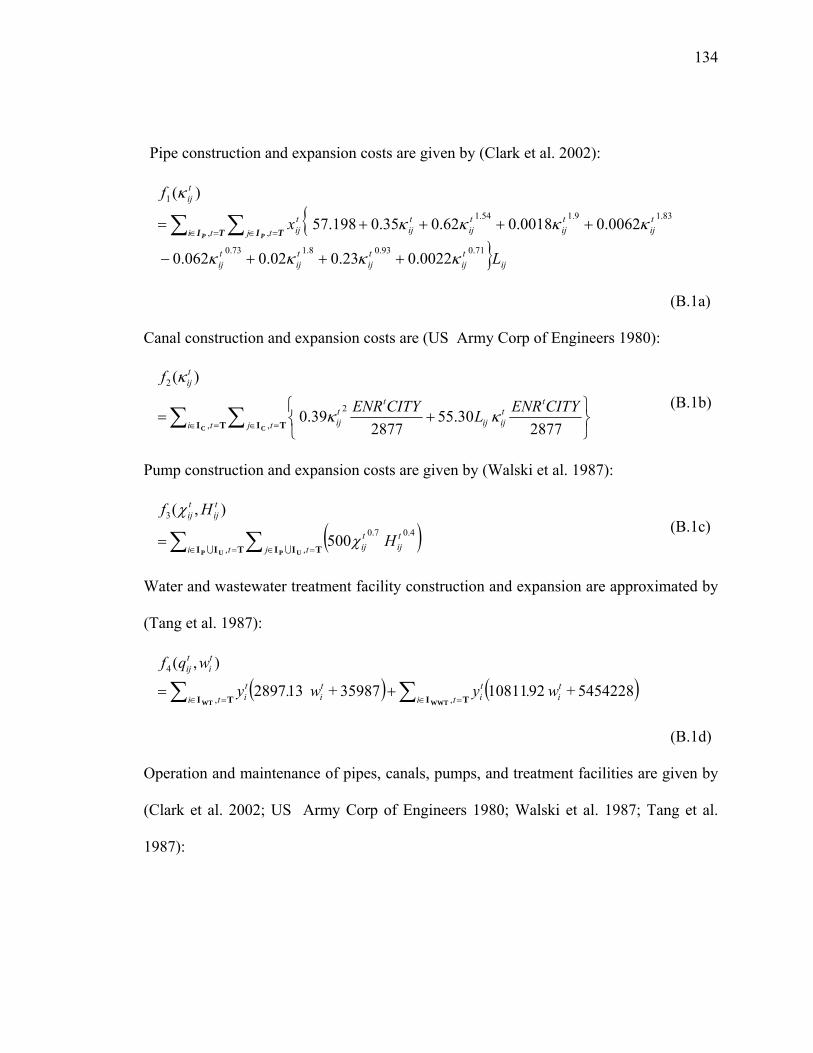
134
Pipe construction and expansion costs are given by (Clark et al. 2002):
ij
tij
tij
tij
tij
ti tjtij
tij
tij
tij
tij
tij
L
x
f
71.093.08.173.0
, ,
83.19.154.1
1
0022.023.002.0062.0
0062.00018.062.035.0198.57
)(
κκκκ
κκκκ
κ
+++−
++++= ∑ ∑=∈ =∈TI TIP P
(B.1a)
Canal construction and expansion costs are (US Army Corp of Engineers 1980):
∑ ∑=∈ =∈⎭⎬⎫
⎩⎨⎧
+=TI TIC Cti tj
ttijij
ttij
tij
CITYENRLCITYENR
f
, ,
2
2
287730.55
287739.0
)(
κκ
κ (B.1b)
Pump construction and expansion costs are given by (Walski et al. 1987):
( )∑ ∑=∈ =∈=
TII TIIUP UPti tjtij
tij
tij
tij
H
Hf
, ,
4.07.0
3
500
),(
U Uχ
χ (B.1c)
Water and wastewater treatment facility construction and expansion are approximated by
(Tang et al. 1987):
( ) ( )∑∑ =∈=∈+=
TITI WWTWT titi
titi
ti
ti
ti
tij
w.yw.y
wqf
,,
4
5454228 + 921081135987 + 132897
),(
(B.1d)
Operation and maintenance of pipes, canals, pumps, and treatment facilities are given by
(Clark et al. 2002; US Army Corp of Engineers 1980; Walski et al. 1987; Tang et al.
1987):
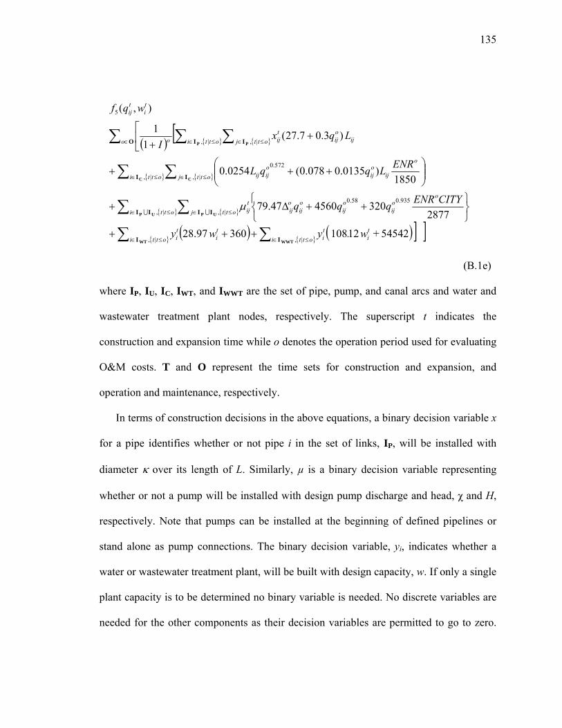
135
( ) [
( ) ( ) ] ]∑∑
∑ ∑
∑ ∑
∑ ∑ ∑
≤∈≤∈
≤∈ ≤∈
≤∈ ≤∈
∈ ≤∈ ≤∈
+++⎭⎬⎫
⎩⎨⎧
++∆+
⎟⎟⎠
⎞⎜⎜⎝
⎛+++
⎢⎣
⎡+
+
ottiti
tiotti
ti
ti
otti ottj
ooij
oij
oij
oij
tij
otti ottj
o
ijoij
oijij
o otti ottj ijoij
tijo
ti
tij
w.ywy
CITYENRqqq
ENRLqqL
LqxI
wqf
|,|,
|, |,
935.058.0
|, |,
572.0
|, |,
5
54542 + 12108 36097.28
2877320456047.79
1850)0135.0078.0(0254.0
)3.07.27(1
1
),(
WWTWT
UP UP
C C
P P
II
II II
I I
O I I
U Uµ
(B.1e)
where IP, IU, IC, IWT, and IWWT are the set of pipe, pump, and canal arcs and water and
wastewater treatment plant nodes, respectively. The superscript t indicates the
construction and expansion time while o denotes the operation period used for evaluating
O&M costs. T and O represent the time sets for construction and expansion, and
operation and maintenance, respectively.
In terms of construction decisions in the above equations, a binary decision variable x
for a pipe identifies whether or not pipe i in the set of links, IP, will be installed with
diameter κ over its length of L. Similarly, µ is a binary decision variable representing
whether or not a pump will be installed with design pump discharge and head, χ and H,
respectively. Note that pumps can be installed at the beginning of defined pipelines or
stand alone as pump connections. The binary decision variable, yi, indicates whether a
water or wastewater treatment plant, will be built with design capacity, w. If only a single
plant capacity is to be determined no binary variable is needed. No discrete variables are
needed for the other components as their decision variables are permitted to go to zero.
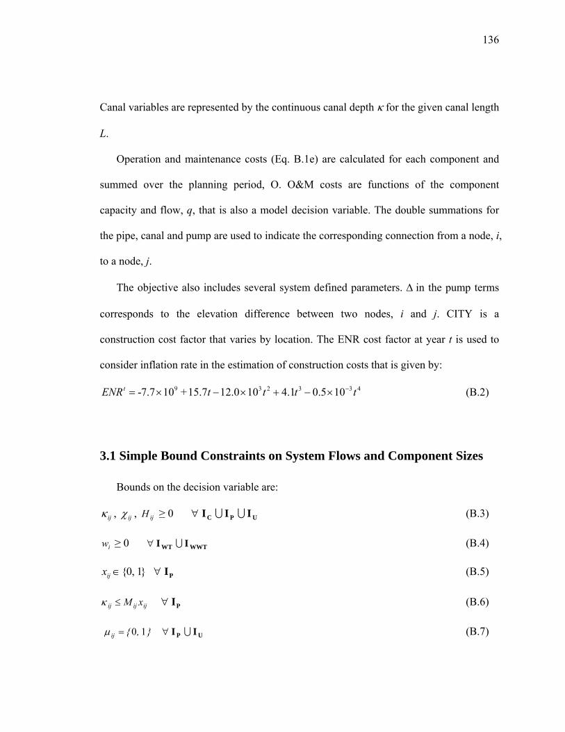
136
Canal variables are represented by the continuous canal depth κ for the given canal length
L.
Operation and maintenance costs (Eq. B.1e) are calculated for each component and
summed over the planning period, O. O&M costs are functions of the component
capacity and flow, q, that is also a model decision variable. The double summations for
the pipe, canal and pump are used to indicate the corresponding connection from a node, i,
to a node, j.
The objective also includes several system defined parameters. ∆ in the pump terms
corresponds to the elevation difference between two nodes, i and j. CITY is a
construction cost factor that varies by location. The ENR cost factor at year t is used to
consider inflation rate in the estimation of construction costs that is given by:
105.01.4100.127.15 +10.77- 433239 ttttENRt −×−+×−×= (B.2)
3.1 Simple Bound Constraints on System Flows and Component Sizes
Bounds on the decision variable are:
ijκ , ijχ , ijH ≥ 0 UPC III UU∀ (B.3)
iw ≥ 0 WWTWT II U∀ (B.4)
1,0∈ijx PI∀ (B.5)
ijijij xM≤κ PI∀ (B.6)
,ij 10=µ UP II U∀ (B.7)
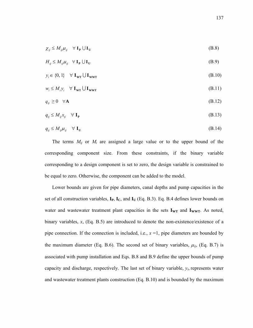
137
ijijij M µχ ≤ UP II U∀ (B.8)
ijijij MH µ≤ UP II U∀ (B.9)
1,0∈iy WWTWT II U∀ (B.10)
iii yMw ≤ WWTWT II U∀ (B.11)
ijq ≥ 0 A∀ (B.12)
ijijij xMq ≤ PI∀ (B.13)
ijijij Mq µ≤ UI∀ (B.14)
The terms Mij or Mi are assigned a large value or to the upper bound of the
corresponding component size. From these constraints, if the binary variable
corresponding to a design component is set to zero, the design variable is constrained to
be equal to zero. Otherwise, the component can be added to the model.
Lower bounds are given for pipe diameters, canal depths and pump capacities in the
set of all construction variables, IP, IC, and IU (Eq. B.3). Eq. B.4 defines lower bounds on
water and wastewater treatment plant capacities in the sets IWT and IWWT. As noted,
binary variables, x, (Eq. B.5) are introduced to denote the non-existence/existence of a
pipe connection. If the connection is included, i.e., x =1, pipe diameters are bounded by
the maximum diameter (Eq. B.6). The second set of binary variables, µij, (Eq. B.7) is
associated with pump installation and Eqs. B.8 and B.9 define the upper bounds of pump
capacity and discharge, respectively. The last set of binary variable, yi, represents water
and wastewater treatment plants construction (Eq. B.10) and is bounded by the maximum
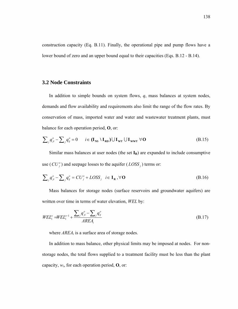
138
construction capacity (Eq. B.11). Finally, the operational pipe and pump flows have a
lower bound of zero and an upper bound equal to their capacities (Eqs. B.12 - B.14).
3.2 Node Constraints
In addition to simple bounds on system flows, q, mass balances at system nodes,
demands and flow availability and requirements also limit the range of the flow rates. By
conservation of mass, imported water and water and wastewater treatment plants, must
balance for each operation period, O, or:
0=− ∑∑ joijj
oji qq WWTWTRDNS II)I\(I UU∈i O∀ (B.15)
Similar mass balances at user nodes (the set IR) are expanded to include consumptive
use ( ojCU ) and seepage losses to the aquifer ( jLOSS ) terms or:
jojj
oijj
oji LOSSCUqq +=− ∑∑ RI∈i , O∀ (B.16)
Mass balances for storage nodes (surface reservoirs and groundwater aquifers) are
written over time in terms of water elevation, WEL by:
i
joijj
ojio
ioi AREA
qqWELWEL
∑∑ −+= −1 (B.17)
where AREAi is a surface area of storage nodes.
In addition to mass balance, other physical limits may be imposed at nodes. For non-
storage nodes, the total flows supplied to a treatment facility must be less than the plant
capacity, wi, for each operation period, O, or:
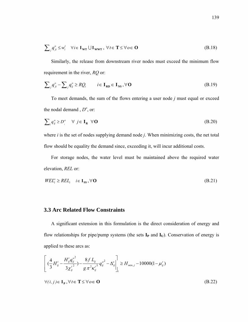
139
tij
oji wq ≤∑ WWTWT II U∈∀i , OT ∈∀≤∈∀ ot (B.18)
Similarly, the release from downstream river nodes must exceed the minimum flow
requirement in the river, RQ or:
ijoijj
oji RQqq ≥− ∑∑ NSRD II ∈∈i , O∀ (B.19)
To meet demands, the sum of the flows entering a user node j must equal or exceed
the nodal demand , Do, or:
∑ ≥i
ooij i
Dq RI∈∀ j O∀ (B.20)
where i is the set of nodes supplying demand node j. When minimizing costs, the net total
flow should be equality the demand since, exceeding it, will incur additional costs.
For storage nodes, the water level must be maintained above the required water
elevation, REL or:
ioi RELWEL ≥ SSI∈i , O∀ (B.21)
3.3 Arc Related Flow Constraints
A significant extension in this formulation is the direct consideration of energy and
flow relationships for pipe/pump systems (the sets IP and IU). Conservation of energy is
applied to these arcs as:
)1(100008
)33
4( ,2
522
2tijjmin
i
oij
oijt
ij
ij
tij
oij
tijt
ij Hqg
LfqHH µ
κπχ−−≥
⎥⎥⎦
⎤
⎢⎢⎣
⎡∆−−−
PI∈∀ )j,i( , OT ∈∀≤∈∀ ot (B.22)
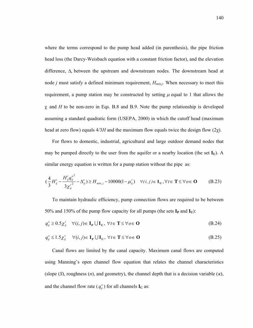
140
where the terms correspond to the pump head added (in parenthesis), the pipe friction
head loss (the Darcy-Weisbach equation with a constant friction factor), and the elevation
difference, ∆, between the upstream and downstream nodes. The downstream head at
node j must satisfy a defined minimum requirement, Hmin,j. When necessary to meet this
requirement, a pump station may be constructed by setting µ equal to 1 that allows the
χ and H to be non-zero in Eqs. B.8 and B.9. Note the pump relationship is developed
assuming a standard quadratic form (USEPA, 2000) in which the cutoff head (maximum
head at zero flow) equals 4/3H and the maximum flow equals twice the design flow (2χ).
For flows to domestic, industrial, agricultural and large outdoor demand nodes that
may be pumped directly to the user from the aquifer or a nearby location (the set IU). A
similar energy equation is written for a pump station without the pipe as:
)1(10000)33
4( ,2
2tijjmin
oijt
ij
oij
tijt
ij HqH
H µχ
−−≥∆−− UI∈∀ )j,i( , OT ∈∀≤∈∀ ot (B.23)
To maintain hydraulic efficiency, pump connection flows are required to be between
50% and 150% of the pump flow capacity for all pumps (the sets IP and IU):
tij
oijq χ5.0≥ UP II U∈∀ ),( ji , OT ∈∀≤∈∀ ot (B.24)
tij
oijq χ5.1≤ UP II U∈∀ ),( ji , OT ∈∀≤∈∀ ot (B.25)
Canal flows are limited by the canal capacity. Maximum canal flows are computed
using Manning’s open channel flow equation that relates the channel characteristics
(slope (S), roughness (n), and geometry), the channel depth that is a decision variable (κ),
and the channel flow rate ( oijq ) for all channels IC as:
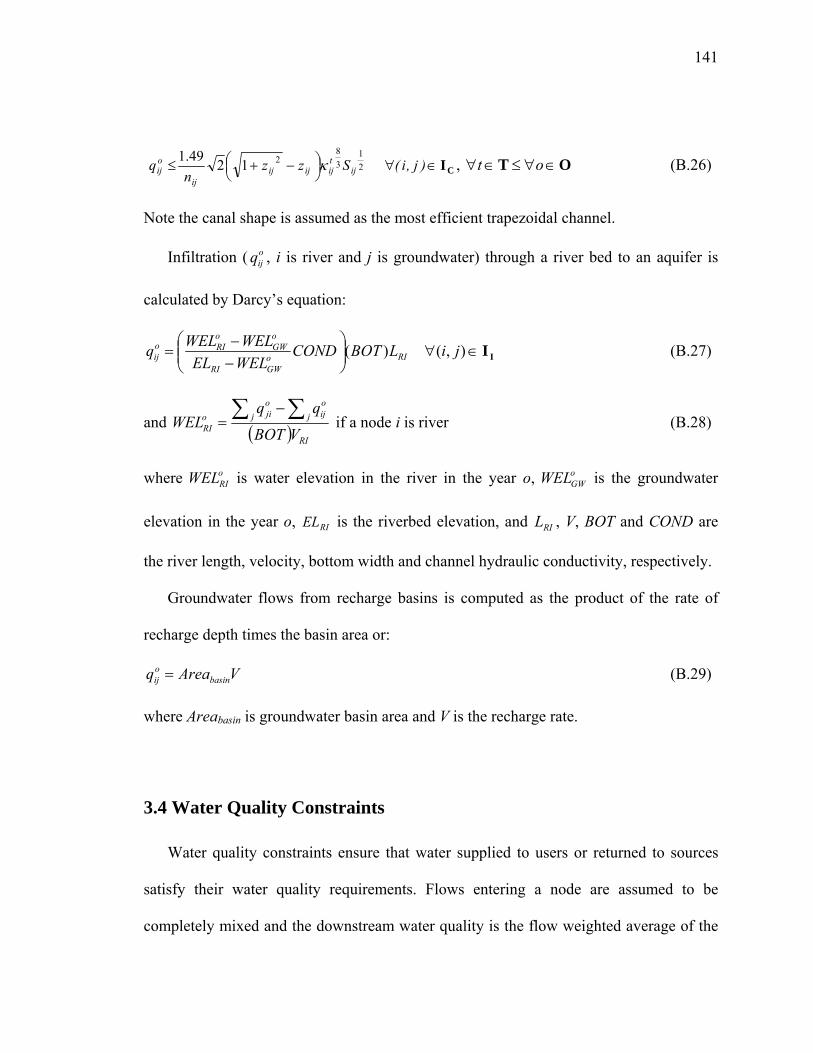
141
21
38
21249.1ij
tijijij
ij
oij Szz
nq κ⎟
⎠⎞⎜
⎝⎛ −+≤ CI∈∀ )j,i( , OT ∈∀≤∈∀ ot (B.26)
Note the canal shape is assumed as the most efficient trapezoidal channel.
Infiltration ( oijq , i is river and j is groundwater) through a river bed to an aquifer is
calculated by Darcy’s equation:
RIoGWRI
oGW
oRIo
ij LBOTCONDWELELWELWELq )(⎟⎟
⎠
⎞⎜⎜⎝
⎛−−
= II∈∀ ),( ji (B.27)
and ( ) RI
joijj
ojio
RI VBOT
qqWEL
∑∑ −= if a node i is river (B.28)
where oRIWEL is water elevation in the river in the year o, o
GWWEL is the groundwater
elevation in the year o, RIEL is the riverbed elevation, and RIL , V, BOT and COND are
the river length, velocity, bottom width and channel hydraulic conductivity, respectively.
Groundwater flows from recharge basins is computed as the product of the rate of
recharge depth times the basin area or:
VAreaq basinoij = (B.29)
where Areabasin is groundwater basin area and V is the recharge rate.
3.4 Water Quality Constraints
Water quality constraints ensure that water supplied to users or returned to sources
satisfy their water quality requirements. Flows entering a node are assumed to be
completely mixed and the downstream water quality is the flow weighted average of the
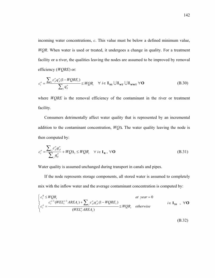
142
incoming water concentrations, c. This value must be below a defined minimum value,
WQR. When water is used or treated, it undergoes a change in quality. For a treatment
facility or a river, the qualities leaving the nodes are assumed to be improved by removal
efficiency (WQRE) or:
ij
oij
ijoji
ojio
i WQRq
WQREqcc ≤
−=
∑∑ )1(
WWTWTNS III UU∈∀ i O∀ (B.30)
where WQRE is the removal efficiency of the contaminant in the river or treatment
facility.
Consumers detrimentally affect water quality that is represented by an incremental
addition to the contaminant concentration, WQ∆. The water quality leaving the node is
then computed by:
iij
oij
joji
ojio
i WQRWQq
qcc ≤∆+=
∑∑
RI∈∀ i , O∀ (B.31)
Water quality is assumed unchanged during transport in canals and pipes.
If the node represents storage components, all stored water is assumed to completely
mix with the inflow water and the average contaminant concentration is computed by:
⎪⎩
⎪⎨
⎧
≤−+
=
=≤
∑−−
otherwiseWQRAREAWEL
WQREqcAREAWELcc
yearatWQRc
ii
oi
ijoji
ojii
oi
oio
i
ii
)(
)1()(0
11
0
SSI∈i , O∀
(B.32)
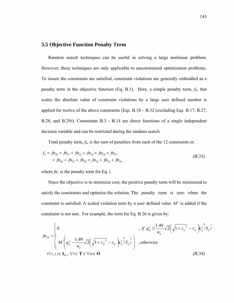
143
3.5 Objective Function Penalty Term
Random search techniques can be useful in solving a large nonlinear problem.
However, these techniques are only applicable to unconstrained optimization problems.
To insure the constraints are satisfied, constraint violations are generally embedded as a
penalty term in the objective function (Eq. B.1). Here, a simple penalty term, f6, that
scales the absolute value of constraint violations by a large user defined number is
applied for twelve of the above constraints (Eqs. B.18 – B.32 (excluding Eqs. B.17, B.27,
B.28, and B.29)). Constraints B.3 - B.14 are direct functions of a single independent
decision variable and can be restricted during the random search.
Total penalty term, f6, is the sum of penalties from each of the 12 constraints or:
343332282726
2524232221206
fnfnfnfnfnfnfnfnfnfnfnfnf++++++
+++++= (B.33)
where fni is the penalty term for Eq. i.
Since the objective is to minimize cost, the positive penalty term will be minimized to
satisfy the constraints and optimize the solution. The penalty term is zero when the
constraint is satisfied. A scaled violation term by a user defined value 'M is added if the
constraint is not met. For example, the term for Eq. B.26 is given by:
⎪⎪⎩
⎪⎪⎨
⎧
⎟⎟⎠
⎞⎜⎜⎝
⎛⎟⎠⎞⎜
⎝⎛ −+−
⎟⎠⎞⎜
⎝⎛ −+≤
=otherwiseSzz
nqM
Szzn
qif
fn
ijtijijij
ij
oij
ijtijijij
ij
oij
,1249.1
1249.1,0
21
38
2'
21
38
2
28
κ
κ
CI∈∀ )j,i( , OT ∈∀≤∈∀ ot (B.34)
144
A single 'M value is applied for all constraints because it is difficult to predict which
constraint will have significant effect on the objective function. For simplicity, this large
factor is not changed during the optimization process.
3.6 Summary of Formulation
The set of equations (Eqs. B.1 - B.32) forms the basis for the water supply
optimization problem. The formulation is general and can consider multiple demand
centers and supply sources, one or more treatment facilities and linkages between users.
Distances and system topography can also be represented. One or more planning periods
can be evaluated with multiple years within each planning period. The decision variables
are a mixture of continuous and binary variables. The equations are highly nonlinear. A
heuristic stochastic search algorithm known as the shuffled frog leaping algorithm
(SFLA) is applied to solve the problem.
4. SHUFFLED FROG LEAPING ALGORITHM (SFLA)
The posed water supply problem is non-linear and non-convex. The degree of
nonlinearity causes difficulties in solving the problem using non-linear programming.
Nonlinear formulation was constructed in MINOS, however, no improvement was
achieved from the initial solutions. Therefore, stochastic search technique, the shuffled
frog leaping algorithm (SFLA) (Eusuff et al., 2006), was applied.
145
SFLA is applicable to problems with continuous and discrete decision variables. It is
a descent based stochastic search method that begins with an initial population of frogs
whose characteristics, known as memes, represent the decision variables.
Memes are units of knowledge that, like an idea, improve as more information is
gained. In a physical domain, memes represent a frog’s position that is improved by
comparing its objective function value with other frogs and changes in a frog’s
characteristics (memes) are made by moving (leaping) in the direction of lower objective
function value in case of minimum problem. In a frog’s domain, he is moving to
locations with higher food concentrations. This movement is similar to the evolution of
an idea that changes as each individual learns something from others.
In SFLA, the total population is partitioned into groups (memeplexes) that search
independently. After a number of iterations, the groups are combined and reformed to
pass information between individuals, similar to the cross-fertilization of ideas between
different organizations. This goal of the overall process is to determine global optimal
solutions. As such, a random component is also included to generate new points that
maintain a diverse search. The process of local group searches and population shuffles
continues until convergence to an optimum is reached or a user-defined number of frogs
have been evaluated.
The global exploration and local search algorithms are presented in the following
steps. This algorithm is slightly modified from Eusuff et al. (2006) in the local search that
extends the potential step size to be beyond the current frog locations. In Eusuff et al, a
new point was limited to fall between the existing frogs.
146
4.1 Global Exploration
Step 0: Initialize: Select m and N, where m = number of memeplexes and N = number of
frogs in each memeplex. Therefore, the total population size in the swamp, F = mN.
Step 1: Generate a virtual population: Sample F virtual frogs U(1), U(2), …, U(F) in the
feasible space dℜ⊂Ω where d is the number of decision variables (i.e., number of
menotype(s) in a meme carried by a frog). The ‘ith’ frog is represented as a vector of
decision variable values U(i) = ),...,,( 21 diii UUU , i = 1, …, F.
Compute the performance value, f(i), for each frog U(i).
Step 2: Rank frogs: Sort the F frogs in order of decreasing performance value in case of
minimum problem. Store them in array X = U(i), f(i), I = 1…F, so that i = 1 represents
the frog with the best performance value. Record the best frog’s position in the entire
population (F frogs), PX, (where PX = U(1)).
Step 3: Partition frogs into memeplexes: Partition array X into m memeplexes Y1, Y2, …,
Ym, each containing n frogs, such that:
mknjjmkfjfjmkUjUjfjUY kkkkk ,...,1],,...,1)),1(()()),1(()(|)(,)([ ==−+=−+==
For example, for m = 3, rank 1 goes to memeplex 1, rank 2 goes to memeplex 2, rank 3
goes to memeplex 3, rank 4 goes to memeplex 1 again, and so on.
Step 4: Memetic evolution within each memeplex: Evolve each memeplex Yk, k = 1, …,
m according to the frog leaping algorithm (FLA) outlined below.
147
Step 5: Shuffle memeplexes: After a defined number of memetic evolutionary steps
within each memeplex, replace Y1, …, Ym into X, such that X = Yk, k = 1, …, m. Sort X
in order of decreasing performance value. Update the population best frog’s position, PX.
Step 6: Check convergence: If the convergence criteria are satisfied, stop. Otherwise,
return to Step 3. Typically, the decision on when to stop is made by a pre-specified
number of consecutive time loops when at least one frog carries the “best memetic
pattern” without change. Alternatively, a maximum total number of function evaluations
can be defined.
4.2 Local Exploration: Frog Leaping Algorithm (FLA)
Step 0: Set im (iteration count) and iN (shuffle count) equal to zero. The number of
iterations and shuffles are limited to user-defined values ic and is, respectively. Form an
initial random set of frogs and evaluate each frogs objective function value.
Step 1: Set im = im + 1.
Step 2: Set iN = iN + 1.
Step 3: Construct a sub-memeplex: The frogs’ goal is to move towards the optimal ideas
by improving their memes. An individual frog is updated using the presently available
information. The new frog is returned to the memeplex and another frog is updated. This
strategy is consistent with evolution of ideas since the best information available is used
unlike a genetic algorithm in which the entire population is updated prior to using any
information gained. To complete this process, a subset of the memeplex, (Yk, k = 1, …,
148
m), called a sub-memeplex, (Ziq, iq = 1, …, q) is considered. Figure B.3 presents the
structure of population, memeplex, and sub-memeplex. The sub-memeplex selection
strategy from a memeplex (Yk) having n frogs is to give higher weights to frogs that have
higher performance values and less weight to those with lower performance values. The
weights are assigned with a triangular probability distribution, i.e.,
pj = 2(n+1-j)/(n(n+1)) , j = 1, ... , n
such that, within a memeplex, (Yk, k = 1, …, m), the frog with best performance has the
highest probability of being selected for the sub-memeplex, p1 = 2/(n+1) and the frog
with worst performance has the lowest probability, pn = 2/(n(n+1)).
Here, q distinct frogs are selected randomly from n frogs in each memeplex (Yk, k =
1, …, m) to form the sub-memeplex array (Ziq, iq = 1, …, q). The sub-memeplex is sorted
so that frogs are arranged in order of decreasing performance. Record the best (iq = 1; iq
= 1, ..., q) and worst (iq = q; iq = 1,…, q) frog’s position in the sub-memeplex as vectors
PB and PW, respectively.
Step 4: Improve the worst frog’s position: When improving a frog’s position, it can adapt
their ideas from the best frog within the memeplex (group), PB, or from the global
(population) best, PX. The direction, step size and new position are first computed for the
frog with worst performance in the sub-memeplex (Ziq, iq = 1, …, q). The computation
includes identifying the direction of improvement (gradient) and the magnitude of change
(step length) in that direction. The direction of change (positive or negative) is defined by
the movement toward the sub-memeplex best or (PB - PW) where P represents the location
vector. This change involves both in magnitude as well as direction of the decisions.
149
The magnitude of the step size is randomly selected as a proportion of change
direction. It is limited by the maximum step size, Smax. The present version of the
algorithm considers a pre-specified fraction of the bound of the variable value as Smax.
Mathematically, the step size is defined as:
Step size, |s| = MIN[2(rand (PB - PW)), Smax ]
where rand is a random number in the range [0,1]. The new position is then computed by:
Z(iq = q) = PW + s (B.35)
Note that the multiplier of 2 in the step size calculation allows the frog’s new position to
be between the two frogs or move beyond the better frog’s location depending on rand.
Then, if the new position is beyond feasible boundary for any decision variable, it is
forced to be the boundary value. This modification improves upon convergence seen in
Eusuff et al (2006).
Compute the new performance value f(iq = q). If the new f(iq = q) is better than the old
f(iq = q), i.e., if the move produces a benefit, then replace the old Z(iq = q) with the new one
and go to Step 7. Otherwise go to Step 5.
Step 5: If Step 4 cannot produce a better result then the step and new position are
computed for that frog by:
Step size, |s| = MIN[2(rand(PX - PW)), Smax ]
and the new position is computed by Eq. B.35.
Compute the new performance value f(iq = q) for point Z(iq = q). If the new f(iq = q) is better
than the old f(iq = q), i.e., if the evolution produces a benefit, then replace the old Z(iq = q)
with new one and go to Step 7. Otherwise go to Step 6.
150
Step 6: Censorship: If the new position is either infeasible or worse than the old position,
the spread of the defective meme is stopped by randomly generating a new frog ‘r’ at a
feasible location to replace the frog whose new position was not favorable to progress.
Compute f(r) and set Z(iq = q) = r and f(iq = q) = f(r).
Step 7: Upgrade the memeplex: After the memetic change for the worst frog in the sub-
memeplex, replace Ziq in their original locations in Yk. Sort Yk in order of decreasing
performance value.
Step 8: If iN < is , go to Step 2.
Step 9: If im < ic , go to Step 1. Otherwise return to global search to shuffle
memeplexes.
Steps 4 and 5 of the FLA are similar in philosophy to particle swarm optimization. A
descent direction is identified for a particular frog and the frog is moved in that direction.
Here, however, since the global search is also introduced in the shuffle operation, only
the local minimum is used rather than the complete population best (Step 4) unless no
improvement is made (Step 5). Since a descent direction is implicitly applied, it may be
fruitful to perform a line search rather than a random step but the simpler approach is
taken here.
151
5. APPLICATIONS
The optimization problem (Eqs. B.1 - B.32) has been formulated for the water supply
systems shown in Figures B.1 and B.2 for 20-year planning periods. New structural
component construction is permitted at the outset (year 1) and new components or
existing component expansion may be added after 10 years. Biochemical Oxygen
Demand (BOD) is used as the representative water quality parameter.
5.1 Single Wastewater Treatment Plant System
The first system to be optimized (Figure B.1) consists single water and wastewater
plants, multiple sources (imported water, groundwater aquifer, and surface water) and
two demands centers (domestic and agricultural). Three types of water transport
structures are used depending upon the connection: canal, pipe and/or pump. All canal
flows for the conveyance of imported and raw water sources are driven by gravity.
Agricultural areas and water treatment plant may directly pump groundwater from
aquifers available near their location so do not require a pipe link. Other flows are
transported through pipes that may require a pump station to supply the energy necessary
to pass flow through the pipeline and satisfy the minimum pressure head requirement at
the outlet (14.0 m of water = 137.9 kPa = 20 psi). Groundwater replenishment through
recharge basins is assumed to occur at a constant rate of 9.1 m/yr (30 ft/yr). Seepage
losses from users to the aquifer are assumed as 0.1% of total user demand.
152
Input parameters for the single wastewater treatment plant system are shown in
Tables B.1 and B.2. The system contains the total of eighteen arcs (Figure B.1). Origin,
destination nodes and arc lengths are listed in Table B.3. As seen in Figure B.1, the
network consists of six canal depth construction decisions (6) and seven pump/pipeline
arcs with their three design decisions (pipe diameter and pump flow capacity and head)
for a total of 21 decisions. The network also includes two pump links for which the pump
design flow and head (four total design decisions) must be selected and two treatment
facilities with plant capacity as decision variables (total of 2 decisions). Thus, 33 design
decision variables are to be determined for each of the two planning periods or a total of
66 design decisions.
Ten of the 18 arc flows in each period are independent control decision variables that
are also selected by the optimization model. The remaining 8 are dependent variables that
are computed from the mass balance constraints defined in Eqs. B.15 and B.16.
Therefore, the final optimization problem contains a total 86 of decision variables for the
two design periods (66 design and 20 control decision variables).
The following SFLA parameters were selected from experience and preliminary
testing: the total number of population (F = 3000), memeplex (m = 10), frogs in each
memeplex (N = 300), evolutionary steps (iN = 300), and frogs in a sub-memeplex (iq =
300) are established and applied in the single wastewater treatment plant system. The
problem was run on a Dell Inspiron with a Centrino Duo T2300 1.6GHz and 1GB of
RAM and was solved in 5.5 min. after 131 thousand function evaluations. Figure B.4
shows the progress of solution with respect to the number of function evaluations. The
153
penalty term that accounts for constraint violations fell dramatically in early iterations
after which the total system cost gradually decreased. Total construction and operation
cost for the single treatment plant system for the 20-year period is $ 771 million (present
value for year 0) or an annual cost of $47 million.
Table B.4 lists the optimal component designs and the optimal network solution is
depicted graphically in Figure B.5. Water and wastewater treatment plant capacities are
0.05 and 0.05 km3/yr during the first design period, respectively. The water and
wastewater treatment plants are not expanded at year 10 suggesting that economies of
scale made oversizing in the first period to be more desirable than future expansion.
Increased transport capacity was required to/from the domestic area in year 10 to
convey the increased demands. Although the flow allocation from the aquifer to the farms
remains constant over time, the groundwater pump capacity was expanded to overcome
the required lift to overcome the drop in the aquifer water level (Table B.5).
The system has abundant amount of water in downstream river and subsurface (Table
B.5) to preserve sustainability. Therefore, the domestic area is supplied mostly from river
through water treatment plant, and pumped water from the aquifer is the main source for
agricultural area.
BOD concentrations in the aquifer and the downstream river remain steady and below
their 30 mg/l water quality requirements (Table B.5). Influents to domestic and
agricultural area also have better quality than the required, 5 mg/l and 30 mg/l,
respectively.
154
As shown in Table B.7, pipe construction is the dominant cost for this system and
economies of scale compel some pipe installations to be constructed in the initial period.
Pipe and pump connections require significant operation costs as compared with the
operation of canal and treatment plants.
5.2 Multiple Wastewater Treatment Plant System
As shown in Figure B.2, multiple water users and wastewater treatment plants are
included in the multiple wastewater treatment plant system in order to investigate a more
generalized system. This network is consists of six users - three domestic areas, one
industrial, one agricultural, and one large outdoor area – and three wastewater treatment
plants. In general, input parameters used for the multiple wastewater treatment plant
system are the same as for the single wastewater treatment plant system except for the
initial population at the domestic areas (Table B.8). Table B.9 summarizes the multiple
wastewater treatment plant system nodal parameters. This network has 44 arc
connections and their lengths are given in Table B.10. The structural design include 6
canals (6 parameters for canal depth), 29 pipes of which pump station could be built
depending on energy relationship (29 parameters for each pipe diameter, pump design
capacity, and pump head), 2 pumps (2 parameters for each pump design capacity and
head), and 4 treatment plants (4 parameters for capacities). The structures can be built or
expanded in year 1 and 10. Total structural design variables are 101 (= 6 + 3 × 29 + 2 × 2
+ 4) for each design period and a total 202 for whole operational period.
155
Flow allocations through twenty-three arcs out of forty four are defined as operation
decision variables while the remaining 21 arcs are dependent variables that are computed
by mass balance equations. In total, the final problem consists of 248 decision variables
(2 design periods × 124 decision variables (101 and 23 for design and operation
variables, respectively)).
The problem was solved using the computer system cited in the previous section in
about 70 minutes and nearly 582 thousands function evaluations. The optimal cost for the
system was $837 million as the present value in the starting year of the planning period
and the estimated annual cost was $51 million. Final optimal solution is depicted in
Figure B. 6. Although the optimal solution found may not be the global optimal solution
due to high discrete nonconvexity associated with the study system, the optimization
process demonstrates the improvement in overall system cost and reduction in the penalty
term (Figure B.7).
Since the system has sufficient local water to meet user demands, imported water is
not purchased. Domestic areas 1 and 2 are supplied from the aquifer which has good
enough water quality to supply domestic demands, and domestic area 3 and industrial
area are supplied from upstream river through water treatment plant.
Pipe, pump, and canal capacities are given in Table B.11. Table B.12 summarizes the
capacities for water and wastewater treatment plants. Canals carry water from the
upstream river to agricultural and large outdoor areas. Large outdoor turf use is partially
supplied with treated wastewater. As for the single treatment plant case, most pipe
construction occurred at the outset due to economies of scale. Pipe construction cost

156
dominates the total system cost (Table B.13). Water quality parameters for influent and
effluent are satisfactory and listed in Table B.14. Water elevation, source discharge,
water demand and population are summarized in Tables B.15 and B.16, respectively.
157
6. CONCLUSIONS
As water demands grow, water supply system capacities must be increased to provide
the desired water. A poorly designed system can waste money and energy. Optimization
of the system can assist decision makers make good decisions to respond to long term
changes. In this study, a large-scale general water supply system optimization model is
developed using deterministic nonlinear programming. The approach was applied to two
moderate and larger hypothetical water networks.
Difficulties in solving the problem using gradient based NLP methods led to the
application of a heuristic stochastic search algorithm, the Shuffled Frog Leaping
Algorithm (SFLA). As the example water communities, the single (7 nodes) and multiple
wastewater treatment plant system (13 nodes) have been optimized in terms of the total
system cost. Total number of decision variables in the single and multiple wastewater
treatment plant system application are 86 and 248, respectively. The resulting annual
minimum costs were $47 million and $51 million, respectively.
The developed single and multiple wastewater treatment plant applications have
sufficient local water to supply user demand, so no external water is purchased.
Economical scale suggests construction of enough treatment and transportation facilities
at the outset in many connections. Pipe construction cost and pipe and pump operation
cost dominates total operation cost. Supply water to user has better quality than the
required and water source keep enough and better quality water to preserve environment.
Further research efforts are needed to develop more detail water supply system, for

158
example, by introducing discrete pipe diameter or uncertainties in the parameters.
Different kind of random search technique such as Shuffled Complex Evolution (SCE)
can be applied and compare the results to find a proper algorithm for the water supply
system.
159
7. NOMENCLATURE
Indices and Sets
N a set of nodes in a network (sources, users, and treatment plants)
A a set of arcs (i, j) from a node i to a node j in a network, N∈∀ ji,
W a set of pollutants
T a set of design period t, 6,1=∈∀ Tt
O a set of operation period t, 6,1=∈∀ Oo
Subsets,
CI a set of canal connections, AIC ⊆
PI a set of pipe connections, AIP ⊆
UI a set of pump connections, AIU ⊆
BI a set of connections through a recharge basin to an aquifer, AIB ⊆
II a set of seepage from users to an aquifer and riverbed infiltration, AII ⊆
RI a set of users, NIR ⊆
SI a set of sources, NIS ⊆
SSI a set of storage sources, NII SSS ⊆⊆
NSI a set of non-storage sources, NII SNS ⊆⊆
IWI imported water, NIII SNSIW ⊆⊆⊆
RUI river upstream node, NIII SNSRU ⊆⊆⊆
160
RDI river downstream node, NIII SNSRD ⊆⊆⊆
WTI a set of water treatment plants, NIWT ⊆
WWTI a set of wastewater treatment plants, NIWWT ⊆
Data
f Darcy Weisbach coefficient
ijn Manning coefficient of pipes and canals from i to j CP II U∀
ijz Channel side slope from i to j CI∀
COND hydraulic conductivity
I interest rate
CITY city multiplier
IWA imported water available
oiPOP population at an operation year o at i RI∈i , O∈o
At year 0, 0iPOP initial population at a node i
ooi POPGRPOPPOP )1(0 +=
oPP precipitation at an operation year o O∈o
iAREA area of a node i if a node i is a storage source SI∈i
iCU consumptive use at a node i N∀
iLOSS seepage loss to an aquifer at a node i N∀
iEL elevation at a node i N∀
ijL length for an arcs (i, j) A∀
161
iREL required water elevation at a node i if a node i is a storage source SI∈i
iRQ required discharge at a node i if a node i is a non-storage source SI∈i
iWQR water quality requirement at a node i SR II U∀
iWQ∆ water quality increasing at a node i RI∀
iWQRE water quality removal efficiency at a node i TS II U∀
0ikc water quality of pollutant k in a node i in year 0 if a node i is a storage source
SSI∈i
BOT river bottom width
LRI river length
VRI average velocity in river
Hmin,j minimum pressure requirement at the end of pipe and pump connections
Areabasin groundwater basin area
V recharge rate
Decision variables
tijx takes value 1 if an arcs (i, j) is built at a design period t
and 0 otherwise CP II U∀ , T∈t
tijµ takes value 1 if a pump in an arcs (i, j) is built at a design period t
and 0 otherwise UP II U∀ , T∈t
tiy takes value 1 if a water and wastewater treatment plant (i) is built at a design period t
and 0 otherwise WWTWT II U∀ , T∈t
162
tijκ pipe diameter [L] or canal depth [L] for an arcs (i, j) at a design period t
CP II U∀ , T∈t
tijχ capacity of pump for an arcs (i, j) [L3/T] at a design period t
UP II U∀ , T∈t
tijH Design head of pump for an arcs (i, j) [L] at a design period t
UP II U∀ , T∈t
oijq flow allocation for an arcs (i, j) at an operation year o [L3/T] A∀ ,
O∈o
tiw capacity at a node i at a design period t [L3] WWTWT II U∀ , T∈t
oijk
c water quality concentration of pollutant k for an arcs (i, j) in an operation year o
oiWEL water table elevation at a node i in an operation year o SI∀ , O∈o
oij∆ elevation differences for the pump installation at an arcs (i, j) in an operation year o
⎪⎩
⎪⎨⎧ ∈
−⎪⎩
⎪⎨⎧ ∈
=otherwiseEL
iifWEL
otherwiseEL
jifWEL
i
oi
j
oj SS II
oijS Channel bottom slope for an arcs (i, j) in an operation year o ⎟
⎟⎠
⎞⎜⎜⎝
⎛ ∆=
ij
oij
L CI∀ ,
O∈o
oi
D demand at a node i in an operation year o RI∀ , O∈o
Indices and sets related to SFLA
U(i) frogs in entire population, i = 1, …, F
163
Yi frogs in a memeplex, i = 1, …, m
Zi frogs in a sub-memeplex, i = 1, …, iq
Data related to SFLA
F total population
M number of memeplexes
N number of frogs in each memeplex
d number of decision variables
im iteration count in frog leaping algorithm
iN shuffle count
Smax maximum step size
ic maximum number of iterations
is maximum number of shuffles
Variables related to SFLA
F(i) performance value of a frog U(i)
PX best frog in entire population F
PB best frog in a sub-memeplex
PW worst frog in a sub-memeplex
s step size
164
8. REFERENCES
Clark, R. M., Sivaganesan, M., Selvakumar, A., and Sethi, V. (2002). “Cost models for
water supply distribution systems.” Journal of Water Resources Planning and
Management, 128(5), 312-321.
Ejeta, M. Z., McGuckin , J. T., and Mays, L. W. (2004). “Market exchange impact on
water supply planning with water quality.” Journal of Water Resources
Planning and Management, 130(6), 439–449.
Eusuff, M., Lansey, K., and Pasha, F. (2006). “Shuffled frog-leaping algorithm: a
memetic meta-heuristic for discrete optimization.” Engineering Optimization,
38(2), 129-154.
Ocanas, G. and Mays, L. W. (1981a). “A model for water reuse planning.” Water
Resources Research, 17(1), 25–32.
Ocanas, G. and Mays, L. W. (1981b). “Water reuse planning models: extensions and
applications.” Water Resources Research, 17(5), 1311-1327.
Tang, C. C., Brill, E. D., and Pfeffer, J. T. (1987). “Optimization techniques for
secondary wastewater treatment system.” Journal of Environmental
Engineering, 113(5), 935-951.
US. Army Corps of Engineers, (1980). Methodology for areawide planning studies.
Engineer Technical. Letter No. 1110-2-502, Washington, D.C.
United States Environmental Protection Agency, (2000). EPANET2 Users Manual.
EPA/600/R-00/057, Cincinnati, OH.

165
Walski, T. M., Brill, E. D., Gessler, J., Goulter, I. C., Jeppson, R. M., Lansey, K., Lee,
H., Liebman, J. C., Mays, L., Morgan, D. R., and Ormsbee, L. (1987). “Battle
of the network models: epilogue.” Journal of Water Resources Planning and
Management, 113(2), 191-203.
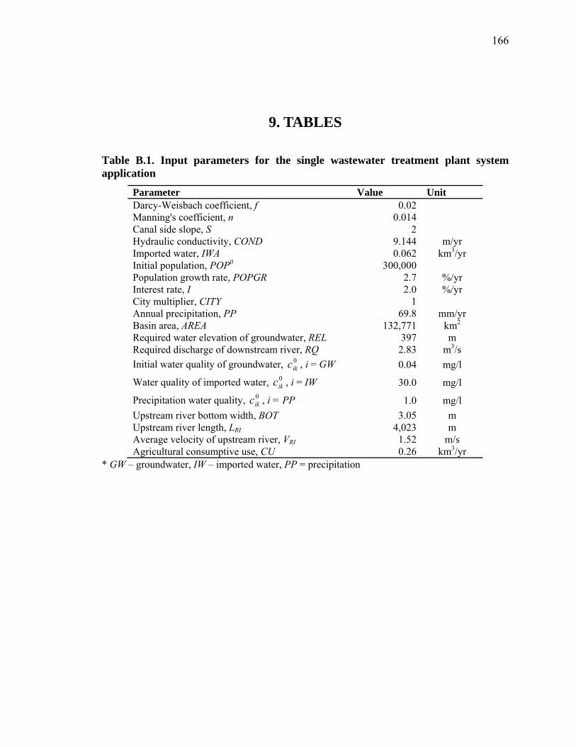
166
9. TABLES
Table B.1. Input parameters for the single wastewater treatment plant system application
Parameter Value Unit Darcy-Weisbach coefficient, f 0.02 Manning's coefficient, n 0.014 Canal side slope, S 2 Hydraulic conductivity, COND 9.144 m/yr Imported water, IWA 0.062 km3/yr Initial population, POP0 300,000 Population growth rate, POPGR 2.7 %/yr Interest rate, I 2.0 %/yr City multiplier, CITY 1 Annual precipitation, PP 69.8 mm/yr Basin area, AREA 132,771 km2 Required water elevation of groundwater, REL 397 m Required discharge of downstream river, RQ 2.83 m3/s Initial water quality of groundwater, 0
ikc , i = GW 0.04 mg/l
Water quality of imported water, 0ikc , i = IW 30.0 mg/l
Precipitation water quality, 0ikc , i = PP 1.0 mg/l
Upstream river bottom width, BOT 3.05 m Upstream river length, LRI 4,023 m Average velocity of upstream river, VRI 1.52 m/s Agricultural consumptive use, CU 0.26 km3/yr
* GW – groundwater, IW – imported water, PP = precipitation
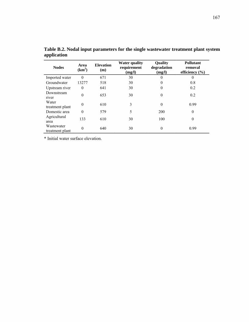
167
Table B.2. Nodal input parameters for the single wastewater treatment plant system application
Nodes Area (km2)
Elevation (m)
Water quality requirement
(mg/l)
Quality degradation
(mg/l)
Pollutant removal
efficiency (%) Imported water 0 671 30 0 0 Groundwater 13277 518 30 0 0.8 Upstream river 0 641 30 0 0.2 Downstream river 0 653 30 0 0.2
Water treatment plant 0 610 3 0 0.99
Domestic area 0 579 5 200 0 Agricultural area 133 610 30 100 0
Wastewater treatment plant 0 640 30 0 0.99
* Initial water surface elevation.
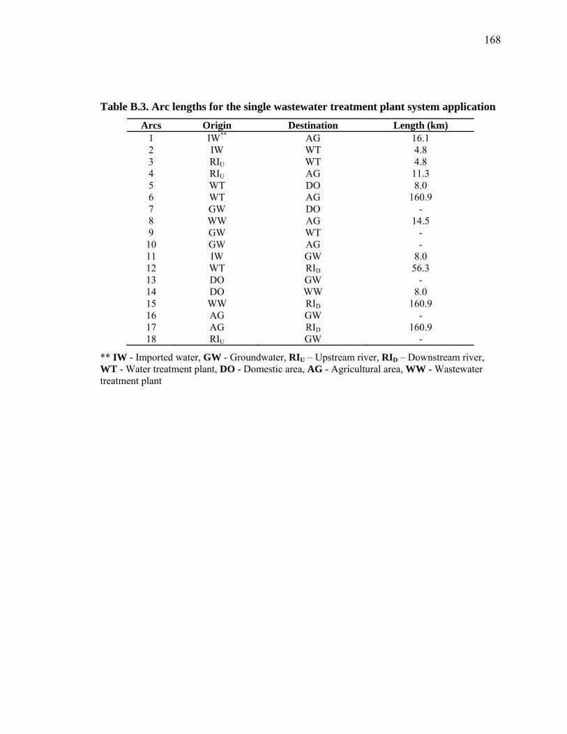
168
Table B.3. Arc lengths for the single wastewater treatment plant system application
Arcs Origin Destination Length (km) 1 IW** AG 16.1 2 IW WT 4.8 3 RIU WT 4.8 4 RIU AG 11.3 5 WT DO 8.0 6 WT AG 160.9 7 GW DO - 8 WW AG 14.5 9 GW WT - 10 GW AG - 11 IW GW 8.0 12 WT RID 56.3 13 DO GW - 14 DO WW 8.0 15 WW RID 160.9 16 AG GW - 17 AG RID 160.9 18 RIU GW -
** IW - Imported water, GW - Groundwater, RIU – Upstream river, RID – Downstream river, WT - Water treatment plant, DO - Domestic area, AG - Agricultural area, WW - Wastewater treatment plant
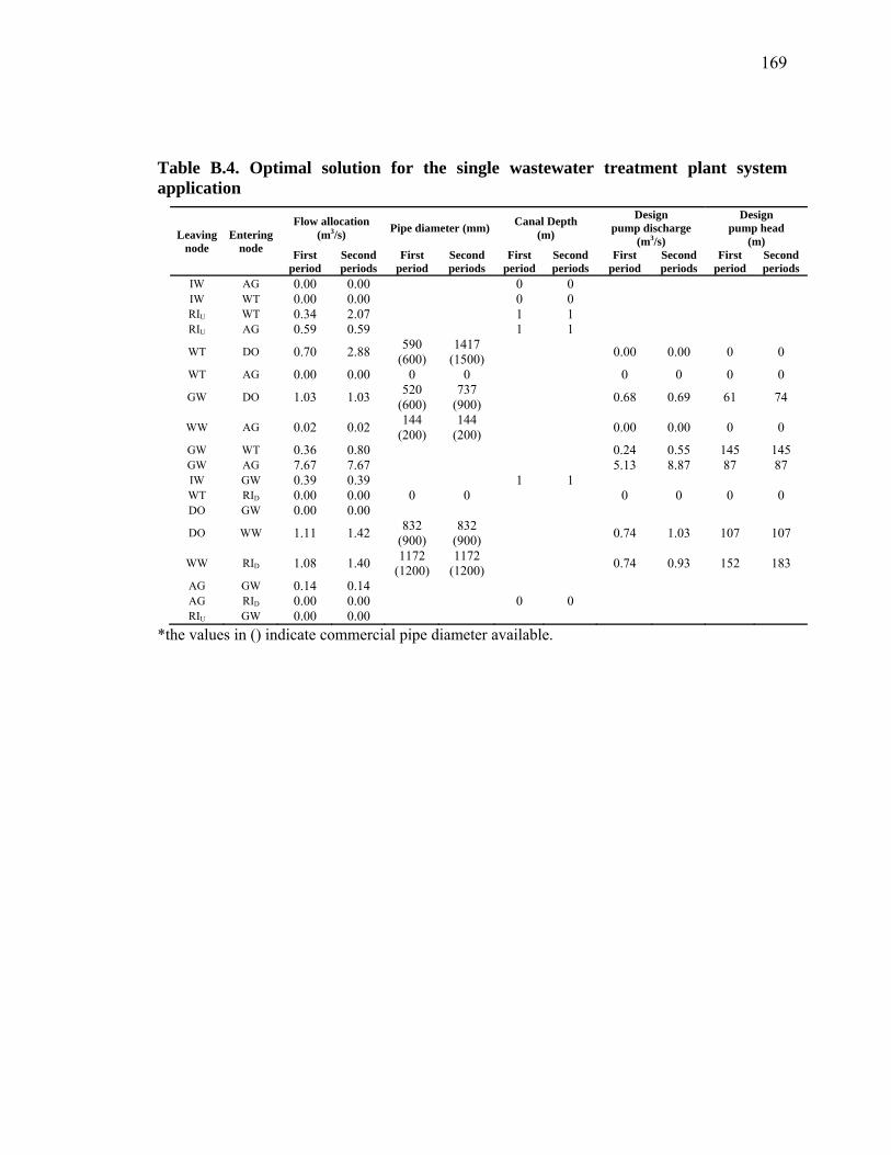
169
Table B.4. Optimal solution for the single wastewater treatment plant system application
Leaving node
Entering node
Flow allocation (m3/s) Pipe diameter (mm) Canal Depth
(m)
Design pump discharge
(m3/s)
Design pump head
(m) First
period Second periods
First period
Second periods
First period
Second periods
First period
Second periods
First period
Second periods
IW AG 0.00 0.00 0 0 IW WT 0.00 0.00 0 0 RIU WT 0.34 2.07 1 1 RIU AG 0.59 0.59 1 1
WT DO 0.70 2.88 590 (600)
1417 (1500) 0.00 0.00 0 0
WT AG 0.00 0.00 0 0 0 0 0 0
GW DO 1.03 1.03 520 (600)
737 (900) 0.68 0.69 61 74
WW AG 0.02 0.02 144 (200)
144 (200) 0.00 0.00 0 0
GW WT 0.36 0.80 0.24 0.55 145 145 GW AG 7.67 7.67 5.13 8.87 87 87 IW GW 0.39 0.39 1 1 WT RID 0.00 0.00 0 0 0 0 0 0 DO GW 0.00 0.00
DO WW 1.11 1.42 832 (900)
832 (900) 0.74 1.03 107 107
WW RID 1.08 1.40 1172 (1200)
1172 (1200) 0.74 0.93 152 183
AG GW 0.14 0.14 AG RID 0.00 0.00 0 0 RIU GW 0.00 0.00
*the values in () indicate commercial pipe diameter available.
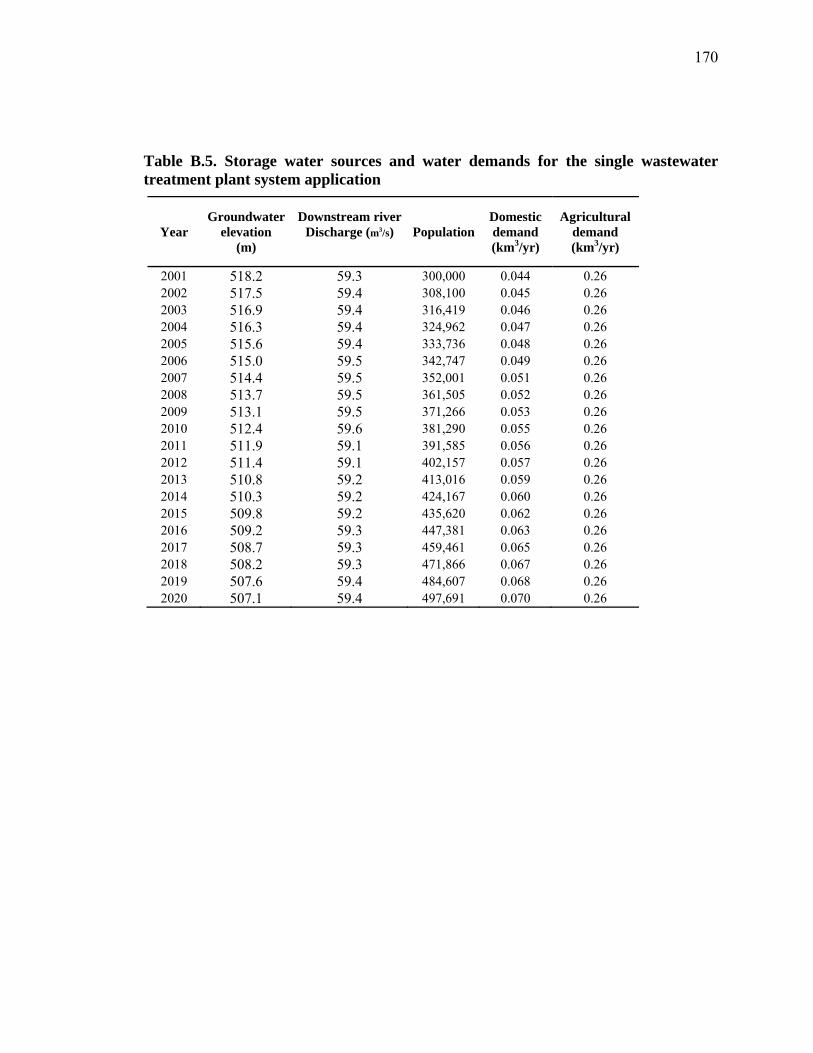
170
Table B.5. Storage water sources and water demands for the single wastewater treatment plant system application
Year Groundwater
elevation (m)
Downstream riverDischarge (m3/s) Population
Domestic demand (km3/yr)
Agricultural demand (km3/yr)
2001 518.2 59.3 300,000 0.044 0.26 2002 517.5 59.4 308,100 0.045 0.26 2003 516.9 59.4 316,419 0.046 0.26 2004 516.3 59.4 324,962 0.047 0.26 2005 515.6 59.4 333,736 0.048 0.26 2006 515.0 59.5 342,747 0.049 0.26 2007 514.4 59.5 352,001 0.051 0.26 2008 513.7 59.5 361,505 0.052 0.26 2009 513.1 59.5 371,266 0.053 0.26 2010 512.4 59.6 381,290 0.055 0.26 2011 511.9 59.1 391,585 0.056 0.26 2012 511.4 59.1 402,157 0.057 0.26 2013 510.8 59.2 413,016 0.059 0.26 2014 510.3 59.2 424,167 0.060 0.26 2015 509.8 59.2 435,620 0.062 0.26 2016 509.2 59.3 447,381 0.063 0.26 2017 508.7 59.3 459,461 0.065 0.26 2018 508.2 59.3 471,866 0.067 0.26 2019 507.6 59.4 484,607 0.068 0.26 2020 507.1 59.4 497,691 0.070 0.26
171
Table B.6. Water quality change (BOD) (mg/l) for the single wastewater treatment plant system application
Year Groundwater Downstream River WT effluent DO influent AG influent WW effluent
2001 0.0* 0.8 0.0 0.0 0.7 2.0 2002 0.0 0.8 0.0 0.0 0.8 2.0 2003 0.0 0.8 0.0 0.0 0.8 2.0 2004 0.0 0.8 0.0 0.0 0.8 2.0 2005 0.0 0.8 0.0 0.0 0.8 2.0 2006 0.0 0.8 0.0 0.0 0.8 2.0 2007 0.0 0.8 0.0 0.0 0.8 2.0 2008 0.0 0.8 0.0 0.0 0.8 2.0 2009 0.0 0.8 0.0 0.0 0.8 2.0 2010 0.0 0.8 0.0 0.0 0.8 2.0 2011 0.0 0.8 0.0 0.0 0.8 2.0 2012 0.0 0.8 0.0 0.0 0.8 2.0 2013 0.0 0.8 0.0 0.0 0.8 2.0 2014 0.0 0.8 0.0 0.0 0.8 2.0 2015 0.0 0.8 0.0 0.0 0.8 2.0 2016 0.0 0.8 0.0 0.0 0.8 2.0 2017 0.0 0.8 0.0 0.0 0.8 2.0 2018 0.0 0.8 0.0 0.0 0.8 2.0 2019 0.0 0.8 0.0 0.0 0.8 2.0 2020 0.0 0.8 0.0 0.0 0.8 2.0
* 0.0 means almost close to 0.0 mg/l.
Table B.7. Construction and operation cost for the single wastewater treatment plant system application
Cost Pipes Pumps Canals Treatment plants Construction (× 106 $) 190.79 26.07 33.59 6.08
Operation at year 1 (× 106 $/yr) 21.22 5.39 0.07 0.06
Expansion (× 106 $) 5.86 2.77 0.00 0.15 Operation at year 10
(× 106 $/yr) 22.72 6.22 0.13 0.06
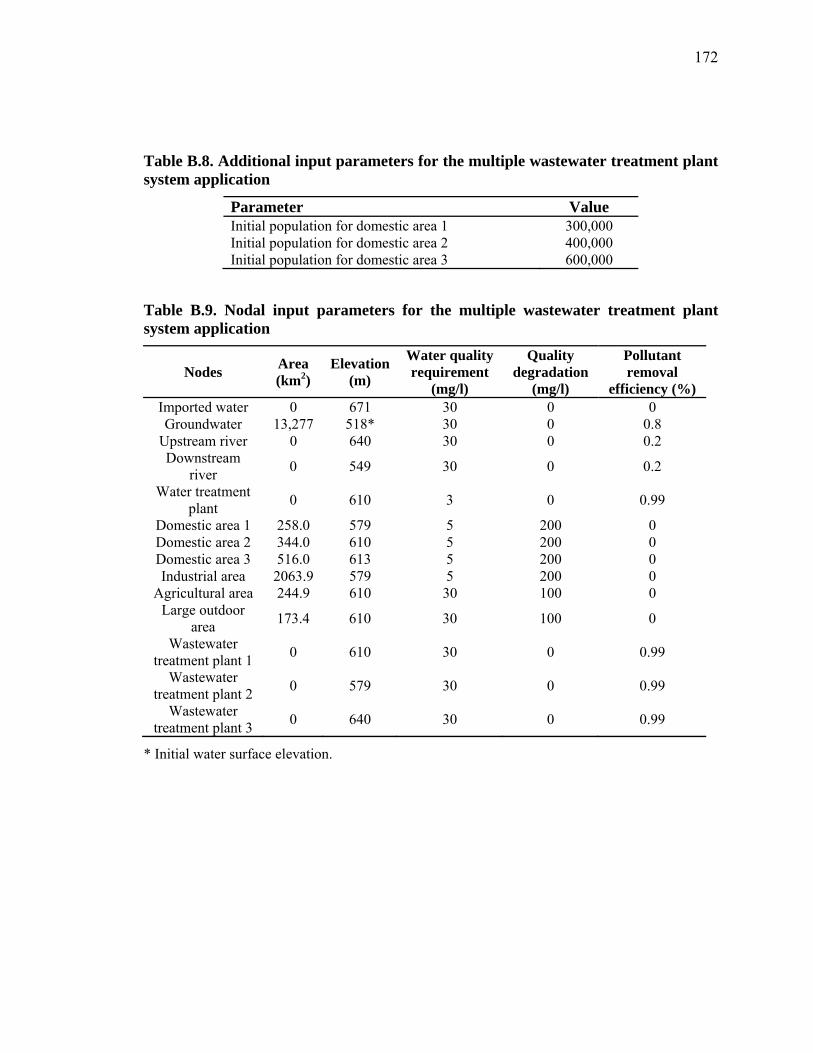
172
Table B.8. Additional input parameters for the multiple wastewater treatment plant system application
Parameter Value Initial population for domestic area 1 300,000 Initial population for domestic area 2 400,000 Initial population for domestic area 3 600,000
Table B.9. Nodal input parameters for the multiple wastewater treatment plant system application
Nodes Area (km2)
Elevation (m)
Water quality requirement
(mg/l)
Quality degradation
(mg/l)
Pollutant removal
efficiency (%) Imported water 0 671 30 0 0 Groundwater 13,277 518* 30 0 0.8
Upstream river 0 640 30 0 0.2 Downstream
river 0 549 30 0 0.2
Water treatment plant 0 610 3 0 0.99
Domestic area 1 258.0 579 5 200 0 Domestic area 2 344.0 610 5 200 0 Domestic area 3 516.0 613 5 200 0 Industrial area 2063.9 579 5 200 0
Agricultural area 244.9 610 30 100 0 Large outdoor
area 173.4 610 30 100 0
Wastewater treatment plant 1 0 610 30 0 0.99
Wastewater treatment plant 2 0 579 30 0 0.99
Wastewater treatment plant 3 0 640 30 0 0.99
* Initial water surface elevation.
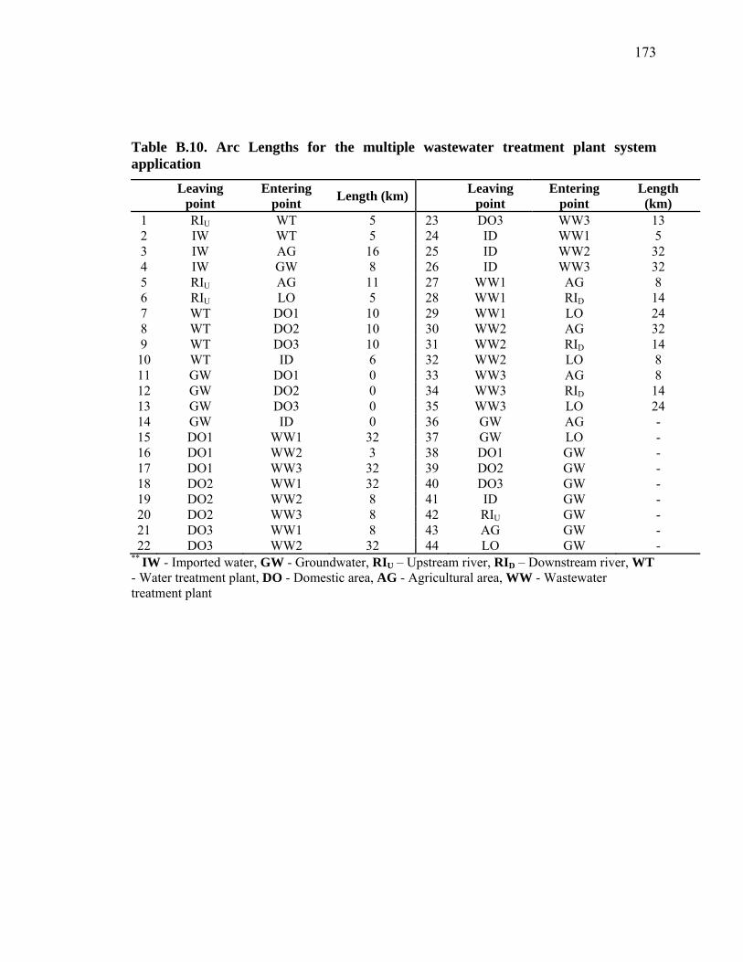
173
Table B.10. Arc Lengths for the multiple wastewater treatment plant system application
Leaving point
Entering point Length (km) Leaving
point Entering
point Length
(km) 1 RIU WT 5 23 DO3 WW3 13 2 IW WT 5 24 ID WW1 5 3 IW AG 16 25 ID WW2 32 4 IW GW 8 26 ID WW3 32 5 RIU AG 11 27 WW1 AG 8 6 RIU LO 5 28 WW1 RID 14 7 WT DO1 10 29 WW1 LO 24 8 WT DO2 10 30 WW2 AG 32 9 WT DO3 10 31 WW2 RID 14 10 WT ID 6 32 WW2 LO 8 11 GW DO1 0 33 WW3 AG 8 12 GW DO2 0 34 WW3 RID 14 13 GW DO3 0 35 WW3 LO 24 14 GW ID 0 36 GW AG - 15 DO1 WW1 32 37 GW LO - 16 DO1 WW2 3 38 DO1 GW - 17 DO1 WW3 32 39 DO2 GW - 18 DO2 WW1 32 40 DO3 GW - 19 DO2 WW2 8 41 ID GW - 20 DO2 WW3 8 42 RIU GW - 21 DO3 WW1 8 43 AG GW - 22 DO3 WW2 32 44 LO GW -
** IW - Imported water, GW - Groundwater, RIU – Upstream river, RID – Downstream river, WT - Water treatment plant, DO - Domestic area, AG - Agricultural area, WW - Wastewater treatment plant
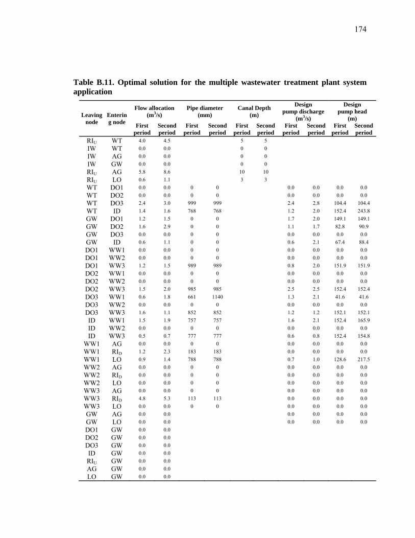
174
Table B.11. Optimal solution for the multiple wastewater treatment plant system application
Leaving node
Entering node
Flow allocation (m3/s)
Pipe diameter (mm)
Canal Depth (m)
Design pump discharge
(m3/s)
Design pump head
(m) First
period Second period
First period
Second period
First period
Second period
First period
Second period
First period
Second period
RIU WT 4.0 4.5 5 5 IW WT 0.0 0.0 0 0 IW AG 0.0 0.0 0 0 IW GW 0.0 0.0 0 0 RIU AG 5.8 8.6 10 10 RIU LO 0.6 1.1 3 3 WT DO1 0.0 0.0 0 0 0.0 0.0 0.0 0.0 WT DO2 0.0 0.0 0 0 0.0 0.0 0.0 0.0 WT DO3 2.4 3.0 999 999 2.4 2.8 104.4 104.4 WT ID 1.4 1.6 768 768 1.2 2.0 152.4 243.8 GW DO1 1.2 1.5 0 0 1.7 2.0 149.1 149.1 GW DO2 1.6 2.9 0 0 1.1 1.7 82.8 90.9 GW DO3 0.0 0.0 0 0 0.0 0.0 0.0 0.0 GW ID 0.6 1.1 0 0 0.6 2.1 67.4 88.4 DO1 WW1 0.0 0.0 0 0 0.0 0.0 0.0 0.0 DO1 WW2 0.0 0.0 0 0 0.0 0.0 0.0 0.0 DO1 WW3 1.2 1.5 989 989 0.8 2.0 151.9 151.9 DO2 WW1 0.0 0.0 0 0 0.0 0.0 0.0 0.0 DO2 WW2 0.0 0.0 0 0 0.0 0.0 0.0 0.0 DO2 WW3 1.5 2.0 985 985 2.5 2.5 152.4 152.4 DO3 WW1 0.6 1.8 661 1140 1.3 2.1 41.6 41.6 DO3 WW2 0.0 0.0 0 0 0.0 0.0 0.0 0.0 DO3 WW3 1.6 1.1 852 852 1.2 1.2 152.1 152.1 ID WW1 1.5 1.9 757 757 1.6 2.1 152.4 165.9 ID WW2 0.0 0.0 0 0 0.0 0.0 0.0 0.0 ID WW3 0.5 0.7 777 777 0.6 0.8 152.4 154.8
WW1 AG 0.0 0.0 0 0 0.0 0.0 0.0 0.0 WW1 RID 1.2 2.3 183 183 0.0 0.0 0.0 0.0 WW1 LO 0.9 1.4 788 788 0.7 1.0 128.6 217.5 WW2 AG 0.0 0.0 0 0 0.0 0.0 0.0 0.0 WW2 RID 0.0 0.0 0 0 0.0 0.0 0.0 0.0 WW2 LO 0.0 0.0 0 0 0.0 0.0 0.0 0.0 WW3 AG 0.0 0.0 0 0 0.0 0.0 0.0 0.0 WW3 RID 4.8 5.3 113 113 0.0 0.0 0.0 0.0 WW3 LO 0.0 0.0 0 0 0.0 0.0 0.0 0.0 GW AG 0.0 0.0 0.0 0.0 0.0 0.0 GW LO 0.0 0.0 0.0 0.0 0.0 0.0 DO1 GW 0.0 0.0 DO2 GW 0.0 0.0 DO3 GW 0.0 0.0 ID GW 0.0 0.0 RIU GW 0.0 0.0 AG GW 0.0 0.0 LO GW 0.0 0.0
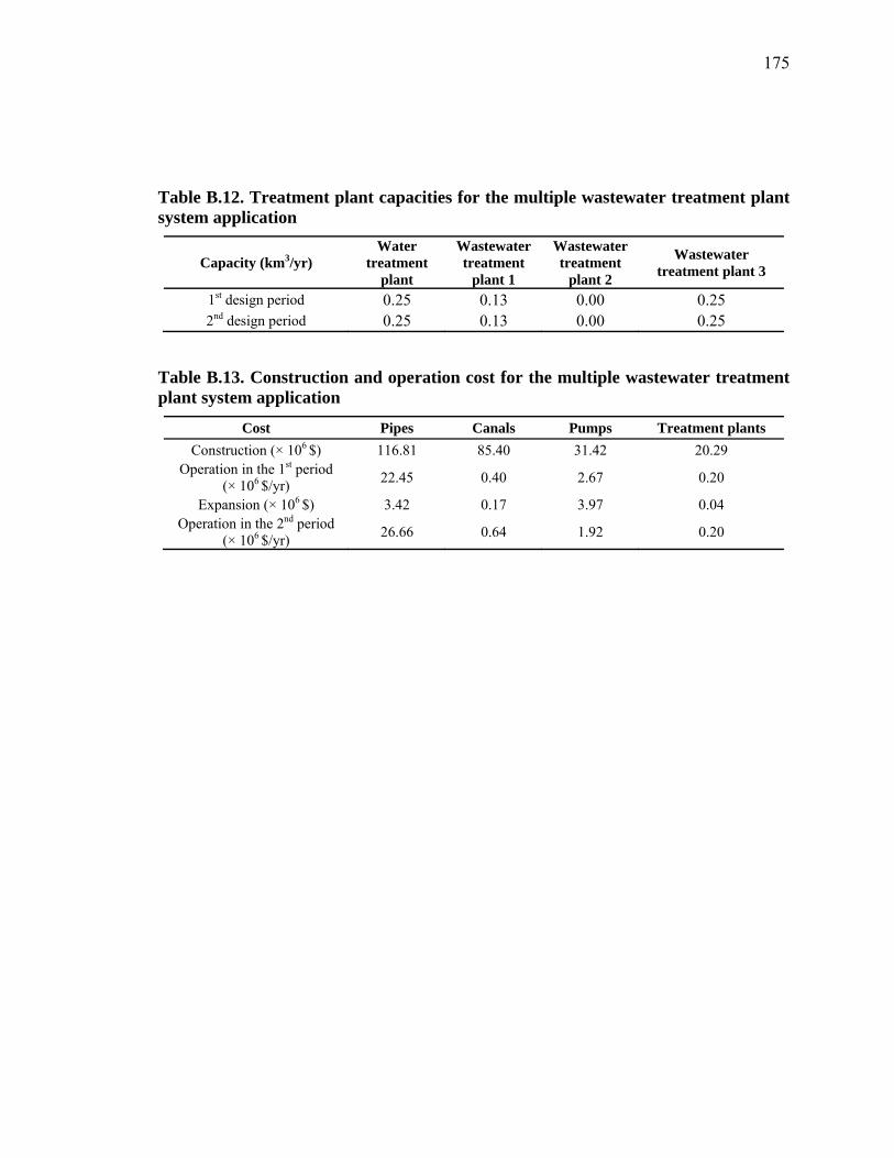
175
Table B.12. Treatment plant capacities for the multiple wastewater treatment plant system application
Capacity (km3/yr) Water
treatment plant
Wastewater treatment
plant 1
Wastewater treatment
plant 2
Wastewater treatment plant 3
1st design period 0.25 0.13 0.00 0.25 2nd design period 0.25 0.13 0.00 0.25
Table B.13. Construction and operation cost for the multiple wastewater treatment plant system application
Cost Pipes Canals Pumps Treatment plants Construction (× 106 $) 116.81 85.40 31.42 20.29
Operation in the 1st period (× 106 $/yr) 22.45 0.40 2.67 0.20
Expansion (× 106 $) 3.42 0.17 3.97 0.04 Operation in the 2nd period
(× 106 $/yr) 26.66 0.64 1.92 0.20
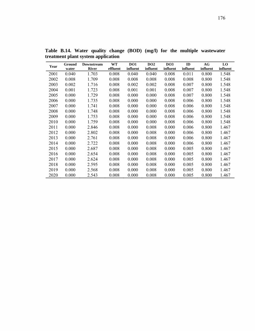
176
Table B.14. Water quality change (BOD) (mg/l) for the multiple wastewater treatment plant system application
Year Ground water
Downstream River
WT effluent
DO1 influent
DO2 influent
DO3 influent
ID influent
AG influent
LO influent
2001 0.040 1.703 0.008 0.040 0.040 0.008 0.011 0.800 1.548 2002 0.008 1.709 0.008 0.008 0.008 0.008 0.008 0.800 1.548 2003 0.002 1.716 0.008 0.002 0.002 0.008 0.007 0.800 1.548 2004 0.001 1.723 0.008 0.001 0.001 0.008 0.007 0.800 1.548 2005 0.000 1.729 0.008 0.000 0.000 0.008 0.007 0.800 1.548 2006 0.000 1.735 0.008 0.000 0.000 0.008 0.006 0.800 1.548 2007 0.000 1.741 0.008 0.000 0.000 0.008 0.006 0.800 1.548 2008 0.000 1.748 0.008 0.000 0.000 0.008 0.006 0.800 1.548 2009 0.000 1.753 0.008 0.000 0.000 0.008 0.006 0.800 1.548 2010 0.000 1.759 0.008 0.000 0.000 0.008 0.006 0.800 1.548 2011 0.000 2.846 0.008 0.000 0.008 0.000 0.006 0.800 1.467 2012 0.000 2.802 0.008 0.000 0.008 0.000 0.006 0.800 1.467 2013 0.000 2.761 0.008 0.000 0.008 0.000 0.006 0.800 1.467 2014 0.000 2.722 0.008 0.000 0.008 0.000 0.006 0.800 1.467 2015 0.000 2.687 0.008 0.000 0.008 0.000 0.005 0.800 1.467 2016 0.000 2.654 0.008 0.000 0.008 0.000 0.005 0.800 1.467 2017 0.000 2.624 0.008 0.000 0.008 0.000 0.005 0.800 1.467 2018 0.000 2.595 0.008 0.000 0.008 0.000 0.005 0.800 1.467 2019 0.000 2.568 0.008 0.000 0.008 0.000 0.005 0.800 1.467 2020 0.000 2.543 0.008 0.000 0.008 0.000 0.005 0.800 1.467
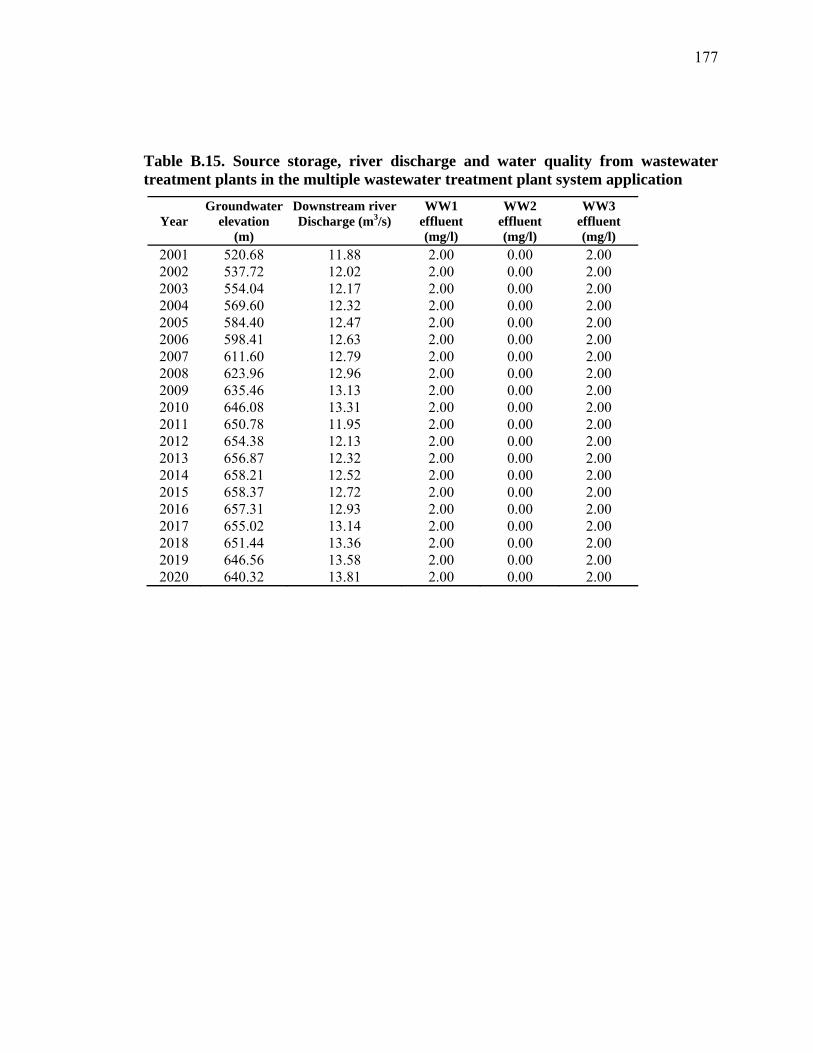
177
Table B.15. Source storage, river discharge and water quality from wastewater treatment plants in the multiple wastewater treatment plant system application
Year Groundwater
elevation (m)
Downstream riverDischarge (m3/s)
WW1 effluent (mg/l)
WW2 effluent (mg/l)
WW3 effluent (mg/l)
2001 520.68 11.88 2.00 0.00 2.00 2002 537.72 12.02 2.00 0.00 2.00 2003 554.04 12.17 2.00 0.00 2.00 2004 569.60 12.32 2.00 0.00 2.00 2005 584.40 12.47 2.00 0.00 2.00 2006 598.41 12.63 2.00 0.00 2.00 2007 611.60 12.79 2.00 0.00 2.00 2008 623.96 12.96 2.00 0.00 2.00 2009 635.46 13.13 2.00 0.00 2.00 2010 646.08 13.31 2.00 0.00 2.00 2011 650.78 11.95 2.00 0.00 2.00 2012 654.38 12.13 2.00 0.00 2.00 2013 656.87 12.32 2.00 0.00 2.00 2014 658.21 12.52 2.00 0.00 2.00 2015 658.37 12.72 2.00 0.00 2.00 2016 657.31 12.93 2.00 0.00 2.00 2017 655.02 13.14 2.00 0.00 2.00 2018 651.44 13.36 2.00 0.00 2.00 2019 646.56 13.58 2.00 0.00 2.00 2020 640.32 13.81 2.00 0.00 2.00
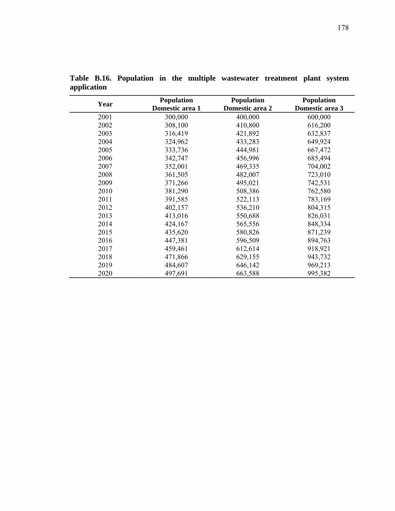
178
Table B.16. Population in the multiple wastewater treatment plant system application
Year Population Domestic area 1
Population Domestic area 2
Population Domestic area 3
2001 300,000 400,000 600,000 2002 308,100 410,800 616,200 2003 316,419 421,892 632,837 2004 324,962 433,283 649,924 2005 333,736 444,981 667,472 2006 342,747 456,996 685,494 2007 352,001 469,335 704,002 2008 361,505 482,007 723,010 2009 371,266 495,021 742,531 2010 381,290 508,386 762,580 2011 391,585 522,113 783,169 2012 402,157 536,210 804,315 2013 413,016 550,688 826,031 2014 424,167 565,556 848,334 2015 435,620 580,826 871,239 2016 447,381 596,509 894,763 2017 459,461 612,614 918,921 2018 471,866 629,155 943,732 2019 484,607 646,142 969,213 2020 497,691 663,588 995,382
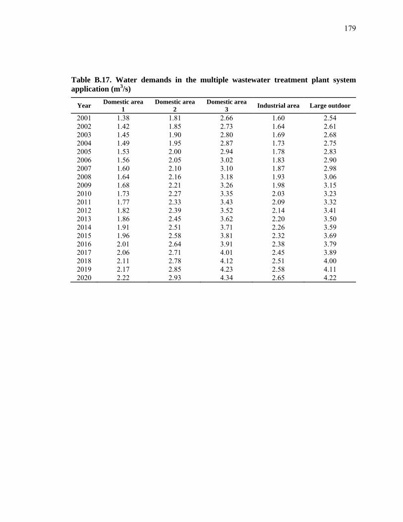
179
Table B.17. Water demands in the multiple wastewater treatment plant system application (m3/s)
Year Domestic area 1
Domestic area 2
Domestic area 3 Industrial area Large outdoor
2001 1.38 1.81 2.66 1.60 2.54 2002 1.42 1.85 2.73 1.64 2.61 2003 1.45 1.90 2.80 1.69 2.68 2004 1.49 1.95 2.87 1.73 2.75 2005 1.53 2.00 2.94 1.78 2.83 2006 1.56 2.05 3.02 1.83 2.90 2007 1.60 2.10 3.10 1.87 2.98 2008 1.64 2.16 3.18 1.93 3.06 2009 1.68 2.21 3.26 1.98 3.15 2010 1.73 2.27 3.35 2.03 3.23 2011 1.77 2.33 3.43 2.09 3.32 2012 1.82 2.39 3.52 2.14 3.41 2013 1.86 2.45 3.62 2.20 3.50 2014 1.91 2.51 3.71 2.26 3.59 2015 1.96 2.58 3.81 2.32 3.69 2016 2.01 2.64 3.91 2.38 3.79 2017 2.06 2.71 4.01 2.45 3.89 2018 2.11 2.78 4.12 2.51 4.00 2019 2.17 2.85 4.23 2.58 4.11 2020 2.22 2.93 4.34 2.65 4.22
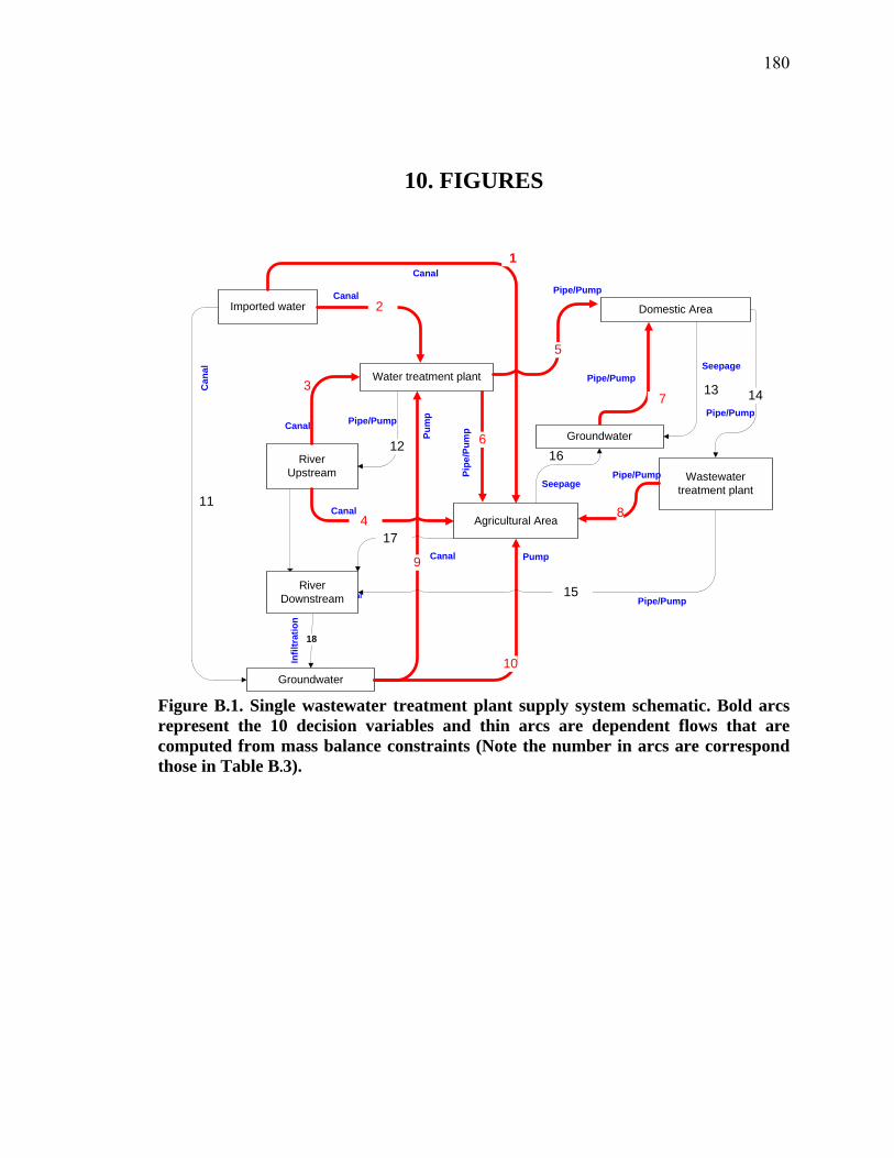
180
10. FIGURES
6
Imported water
RiverUpstream
Groundwater
Domestic Area
Agricultural Area
Wastewater treatment plant
1
200
3Water treatment plant
400
5
7
8
9
10
11
12
13 14
1500
18
1700
Canal
Canal
Canal
Canal
Pipe/Pump
Pipe
/Pum
p
Pipe/Pump
Pipe/Pump
Pum
p
Pump
Pipe/Pump
Seepage
Pipe/Pump
Pipe/PumpCanal
Infil
trat
ion
Can
al
16
Seepage
RiverDownstream
Groundwater
Canal
Figure B.1. Single wastewater treatment plant supply system schematic. Bold arcs represent the 10 decision variables and thin arcs are dependent flows that are computed from mass balance constraints (Note the number in arcs are correspond those in Table B.3).
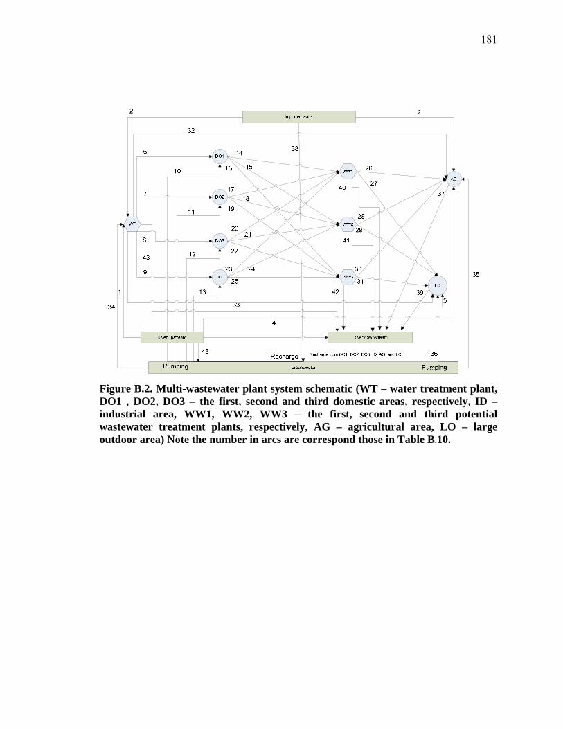
181
Figure B.2. Multi-wastewater plant system schematic (WT – water treatment plant, DO1 , DO2, DO3 – the first, second and third domestic areas, respectively, ID – industrial area, WW1, WW2, WW3 – the first, second and third potential wastewater treatment plants, respectively, AG – agricultural area, LO – large outdoor area) Note the number in arcs are correspond those in Table B.10.
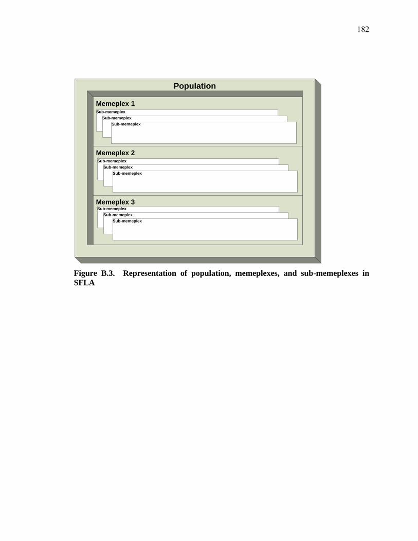
182
Population
Memeplex 1
Memeplex 2
Memeplex 3
Sub-memeplexSub-memeplex
Sub-memeplex
Sub-memeplexSub-memeplex
Sub-memeplex
Sub-memeplexSub-memeplex
Sub-memeplex
Figure B.3. Representation of population, memeplexes, and sub-memeplexes in SFLA
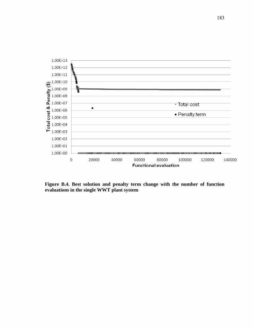
183
Figure B.4. Best solution and penalty term change with the number of function evaluations in the single WWT plant system
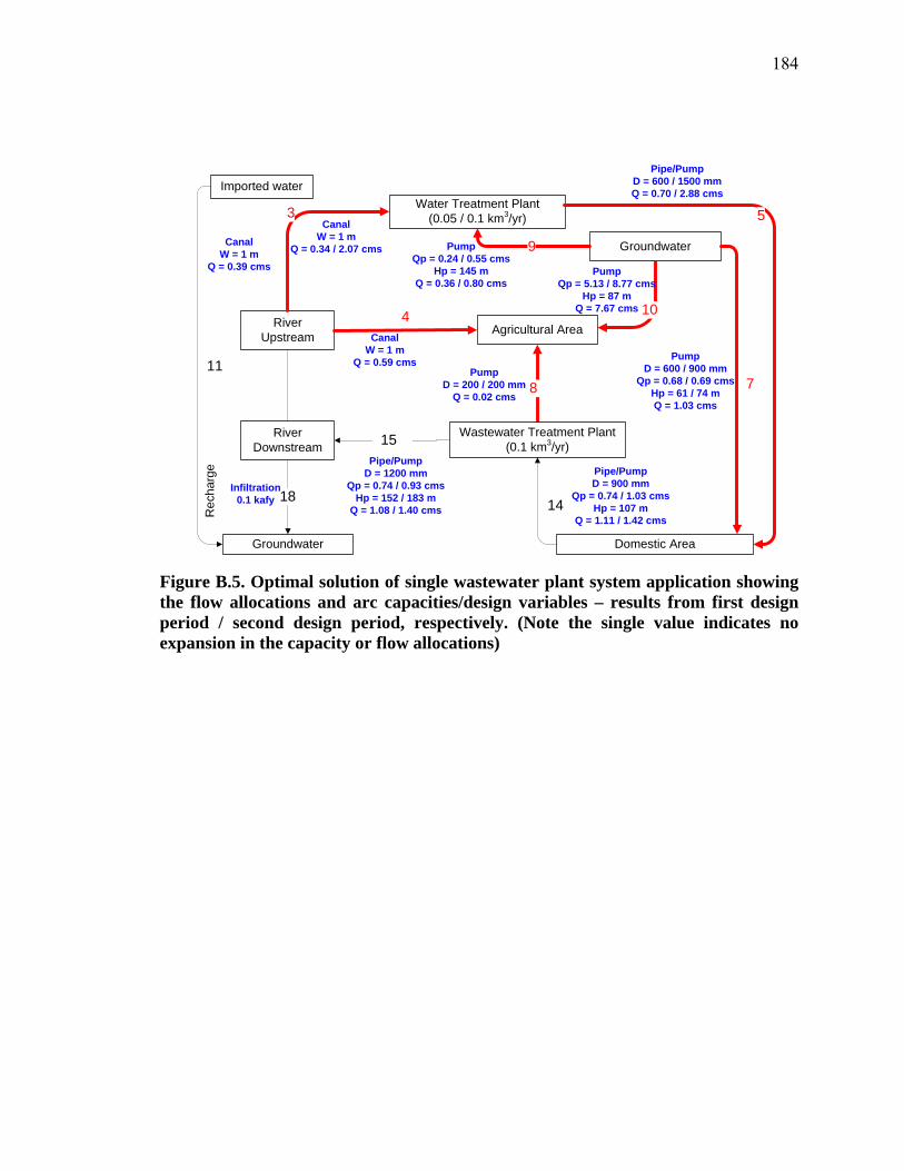
184
800
Imported water
River Upstream
Groundwater Domestic Area
Agricultural Area
Wastewater Treatment Plant (0.1 km3/yr)
11
14
1500
Pipe/PumpD = 600 / 1500 mmQ = 0.70 / 2.88 cms
Pipe/PumpD = 900 mm
Qp = 0.74 / 1.03 cmsHp = 107 m
Q = 1.11 / 1.42 cms
Water Treatment Plant (0.05 / 0.1 km3/yr)3
CanalW = 1 m
Q = 0.34 / 2.07 cms
5
10
Groundwater
PumpQp = 5.13 / 8.77 cms
Hp = 87 mQ = 7.67 cms
Pipe/PumpD = 1200 mm
Qp = 0.74 / 0.93 cmsHp = 152 / 183 m
Q = 1.08 / 1.40 cms
CanalW = 1 m
Q = 0.39 cms
18Infiltration
0.1 kafy
Rec
harg
e
River Downstream
4Canal
W = 1 mQ = 0.59 cms
7
PumpD = 600 / 900 mm
Qp = 0.68 / 0.69 cmsHp = 61 / 74 mQ = 1.03 cms
PumpD = 200 / 200 mm
Q = 0.02 cms
9PumpQp = 0.24 / 0.55 cms
Hp = 145 mQ = 0.36 / 0.80 cms
Figure B.5. Optimal solution of single wastewater plant system application showing the flow allocations and arc capacities/design variables – results from first design period / second design period, respectively. (Note the single value indicates no expansion in the capacity or flow allocations)
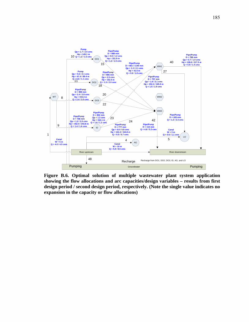
185
Groundwater
WT
WW1
WW2
WW3
DO1
DO2
DO3
ID
AG
LO1
4 5
8
9
Pumping
15
18
20
24
27
PumpingRecharge
48 Recharge from DO1, DO2, DO3, ID, AG, and LO
River downstreamRiver upstream
CanalW = 5 m
Q = 4.0 / 4.5 cms CanalW = 10 m
Q = 5.8 / 8.6 cms
CanalW = 3 m
Q = 0.6 / 1.1 cms
Pipe/PumpD = 999 mm
Qp = 2.4 / 2.8 cmsHp = 104.4 m
Q = 2.4 / 3.0 cms
Pipe/PumpD = 989 mm
Qp = 0.8 / 1.2 cmsHp = 151.9 m
Q = 1.2 / 1.5 cmsPipe/Pump
D = 661 / 1140 mmQp = 1.3 / 2.1 cms
Hp = 41.6 mQ = 0.6 / 1.8 cms
Pipe/PumpD = 788 mm
Qp = 0.7 / 1.0 cmsHp = 128.6 / 217.5 m
Q = 0.9 / 1.4 cms
Pipe/PumpD = 183 mm
Q = 1.2 / 2.3 cmsPipe/PumpD = 768 mm
Qp = 1.2 / 2.0 cmsHp = 152.4 / 243.8 m
Q = 1.4 / 1.6 cms
10
PumpQp = 1.7 / 2.0 cms
Hp = 149.1 mQ = 1.2 / 1.5 cms
11
PumpQp = 0.6 / 2.1 cmsHp = 67.4 / 88.4 mQ = 0.6 / 1.1 cms
Pipe/PumpD = 985 mm
Qp = 2.5 cmsHp = 152.4 m
Q = 1.5 / 2.0 cms
22
Pipe/PumpD = 852 mm
Qp = 1.2 cmsHp = 152.1 m
Q = 1.6 / 1.1 cms
23
Pipe/PumpD = 757 mm
Qp = 1.6 / 2.1 cmsHp = 152.4 / 165.9 m
Q = 1.5 / 1.9 cms
Pipe/PumpD = 777 mm
Qp = 0.6 / 0.8 cmsHp = 152.4 / 154.8 m
Q = 0.5 / 0.7 cms
40
42Pipe/PumpD = 113 mm
Q = 4.8 / 5.3 cms
Figure B.6. Optimal solution of multiple wastewater plant system application showing the flow allocations and arc capacities/design variables – results from first design period / second design period, respectively. (Note the single value indicates no expansion in the capacity or flow allocations)
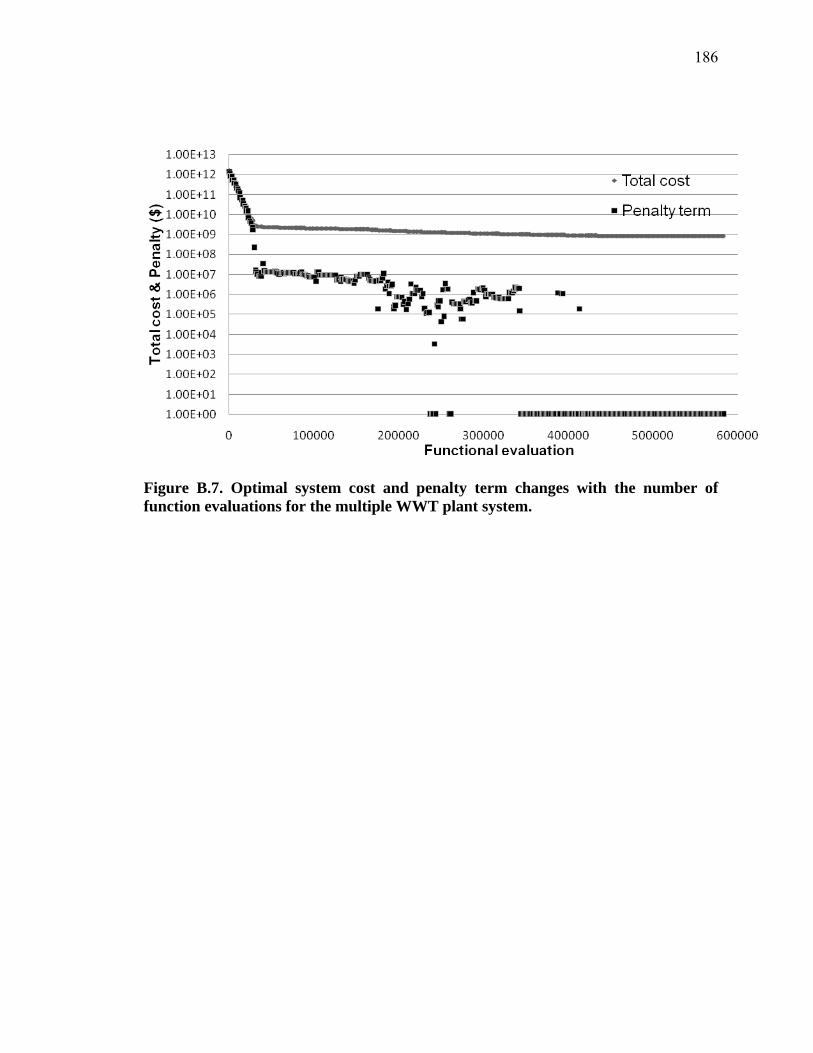
186
Figure B.7. Optimal system cost and penalty term changes with the number of function evaluations for the multiple WWT plant system.

187
APPENDIX C: RELIABLE WATER SUPPLY SYSTEM
DESIGN UNDER UNCERTAINTY
C. Graph
188
Reliable Water Supply System Design under Uncertainty
G. Chung1, K. Lansey2, and G. Bayraksan3
ABSTRACT
Long term reliability is the most important design factor for water supply systems. Water
supply systems are particularly impacted by uncertain future conditions. Many research
efforts have attempted to account for data uncertainty while simultaneously improving
economical feasibility and attaining system reliability. However, the large problem size
and the correlated uncertainties make solving the problem difficult to solve. To consider
correlated uncertainties in water demand and supply, this study applies the robust
optimization approach of Bertsimas and Sim to a water supply system design problem.
Robust optimization aims to find a solution that remains feasible under data
uncertainty. For instance, a water supply system will be “robust” so that it can meet
demand under extreme drought conditions. However, such a system can be too
conservative and costly. It is possible to vary the degree of conservatism to allow for a
decision maker to understand the trade-off between system reliability and economical
feasibility/cost.
In this study, the uncertainty factors are controlled by the degree of conservatism such
that the system stability is guaranteed under uncertain conditions. The degree of
1Graduate Student, Department of Civil Engineering and Engineering Mechanics, The University of Arizona, Tucson, AZ 85721, USA (Tel: 1-520-360-9554, E-mail: [email protected]) 2 Professor, Department of Civil Engineering and Engineering Mechanics, The University of Arizona, Tucson, AZ 85721, USA (Tel: 1-520-621-2512, Fax: 1-520-621-2550, E-mail: [email protected]) 3 Assistant Professor, Department of Systems Industrial Engineering, The University of Arizona, Tucson, AZ 85721, USA (Tel: 1-520-621-2605, E-mail: [email protected] )

189
conservatism is presented as a form of the probability bound of constraint violation. As a
result, the total cost increases as the degree of conservatism is increased, i.e., the
probability bound of constraint violation is decreased. A trade-off appears to exist
between the level of conservatism and imported water purchase, i.e., cost increase. It was
found that the robust optimization approach can be a useful tool to find a solution that
prevents system failure at a certain level of risk within the available budget.
190
1. INTRODUCTION
A municipal water supply system is defined as the physical infrastructure to treat,
deliver water to and collect water from users. The capacities of alternative components
are based upon predictions of future population and climatic conditions. Uncertainty in
predicting these conditions is inherent in all water supply systems. Thus, to reduce the
risk of failure during future operations, it is desirable to consider these uncertainties
during the planning process. A decision made with a deterministic model may result in
two consequences; lower net benefits than expected (i.e., it is more costly to provide the
desired water) or some probability of system failure, where failure is defined as not
meeting a given demand or other system constraint (Watkins and McKinney 1997).
These consequences may be rectified in real-time operations at some cost but flexibility
must be built into the system during the design process to allow for those adjustments.
Deterministic optimization that is based on satisfying demand/supply conditions without
consideration of uncertainty removes this flexibility. Thus, a reliability-based design tool
is needed that can assist decision makers plan a long-term water supply scheme to cope
with the future changes in water demands and supplies.
The complexity of the system and the correlated uncertainties make incorporating
uncertainty a challenging exercise. A number of stochastic optimization approaches have
been applied to water supply system design and operation. Most works have adopted
multi-stage linear or nonlinear optimization techniques. The main objectives of these
studies were to minimize expected total cost for water transfer to spot-markets (Lund and

191
Israel 1995); to develop long- as well as short-term water supply management strategies
(Wilchfort and Lund 1997); to manage water supply capacity under water shortage
conditions (Jenkins and Lund 2000); and to design and operate a water supply system
(Elshorbagy et al. 1997).
Some water supply optimization studies have considered the aspect of system failure
risk. For example, Fiering and Matalas (1990) investigated the robustness of water supply
planning with respect to global climate change for regions where water storage capacity
is limited. Watkins and McKinney (1997) considered uncertainty factors by introducing
the standard deviation of the objective function as a constraint into a two-stage stochastic
model by Lund and Israel (1995). This is embedded in the robust optimization framework
of Mulvey et al. (1995).
Chance constraint modeling intends to limit decisions more directly by considering
uncertainty in model input. For instance, chance constraint model may explicitly limit the
probability of not being able to meet a constraint. Chance constraint models, while
intuitively easy to model, are usually non-convex causing difficulties in optimization and
the approach requires numerical integration of the probability distribution or, if an
invertible probability distribution is assumed to hold, has difficulty considering parameter
correlations.
In this paper, the robust optimization framework of Bertsimas and Sim (2004) is used
to develop a reliable water supply system design. A robust solution can be defined as one
that remains feasible under uncertainty. This type of robust optimization was first
introduced by Soyster (1973) to solve linear programming problems. Soyster’s model,
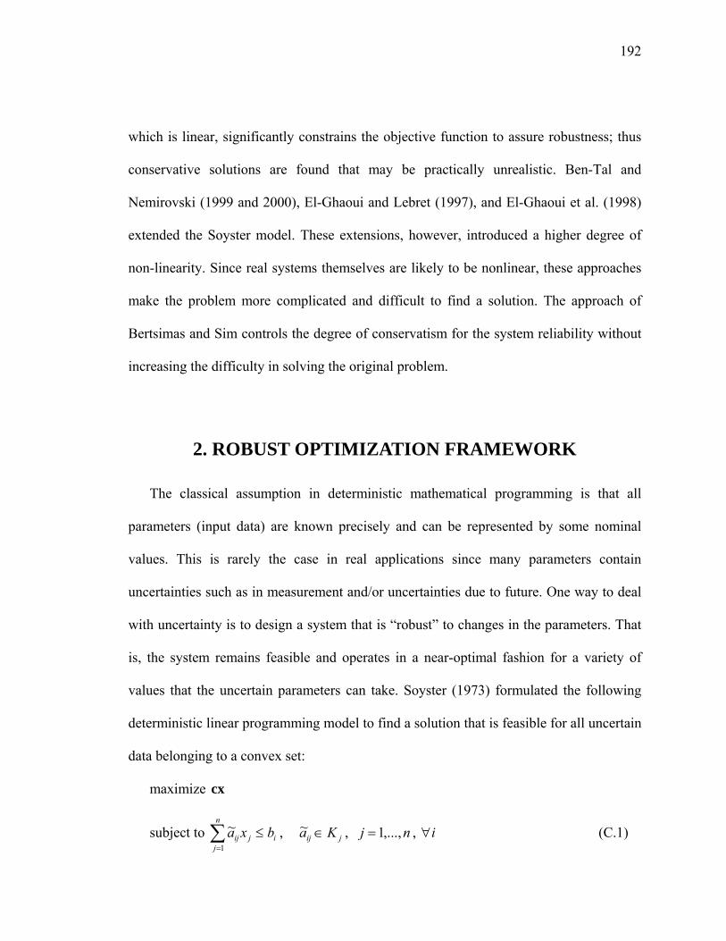
192
which is linear, significantly constrains the objective function to assure robustness; thus
conservative solutions are found that may be practically unrealistic. Ben-Tal and
Nemirovski (1999 and 2000), El-Ghaoui and Lebret (1997), and El-Ghaoui et al. (1998)
extended the Soyster model. These extensions, however, introduced a higher degree of
non-linearity. Since real systems themselves are likely to be nonlinear, these approaches
make the problem more complicated and difficult to find a solution. The approach of
Bertsimas and Sim controls the degree of conservatism for the system reliability without
increasing the difficulty in solving the original problem.
2. ROBUST OPTIMIZATION FRAMEWORK
The classical assumption in deterministic mathematical programming is that all
parameters (input data) are known precisely and can be represented by some nominal
values. This is rarely the case in real applications since many parameters contain
uncertainties such as in measurement and/or uncertainties due to future. One way to deal
with uncertainty is to design a system that is “robust” to changes in the parameters. That
is, the system remains feasible and operates in a near-optimal fashion for a variety of
values that the uncertain parameters can take. Soyster (1973) formulated the following
deterministic linear programming model to find a solution that is feasible for all uncertain
data belonging to a convex set:
maximize cx
subject to ∑=
≤n
jijij bxa
1
~ , jij Ka ∈~ , nj ,...,1= , i∀ (C.1)
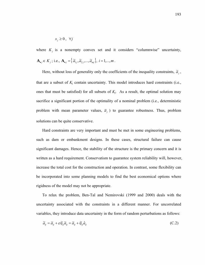
193
0≥jx , j∀
where jK is a nonempty convex set and it considers “columnwise” uncertainty,
jj K∈•A ; i.e., mjjjj aaa ~,...,~,~21=•A , mi ,...,1= .
Here, without loss of generality only the coefficients of the inequality constraints, ja~ ,
that are a subset of Kj contain uncertainty. This model introduces hard constraints (i.e.,
ones that must be satisfied) for all subsets of Kj. As a result, the optimal solution may
sacrifice a significant portion of the optimality of a nominal problem (i.e., deterministic
problem with mean parameter values, ja ) to guarantee robustness. Thus, problem
solutions can be quite conservative.
Hard constraints are very important and must be met in some engineering problems,
such as dam or embankment designs. In these cases, structural failure can cause
significant damages. Hence, the stability of the structure is the primary concern and it is
written as a hard requirement. Conservatism to guarantee system reliability will, however,
increase the total cost for the construction and operation. In contrast, some flexibility can
be incorporated into some planning models to find the best economical options where
rigidness of the model may not be appropriate.
To relax the problem, Ben-Tal and Nemirovski (1999 and 2000) deals with the
uncertainty associated with the constraints in a different manner. For uncorrelated
variables, they introduce data uncertainty in the form of random perturbations as follows:
ijijijijijijij aaaaa ˆ~~~ ηηε +=+= (C.2)
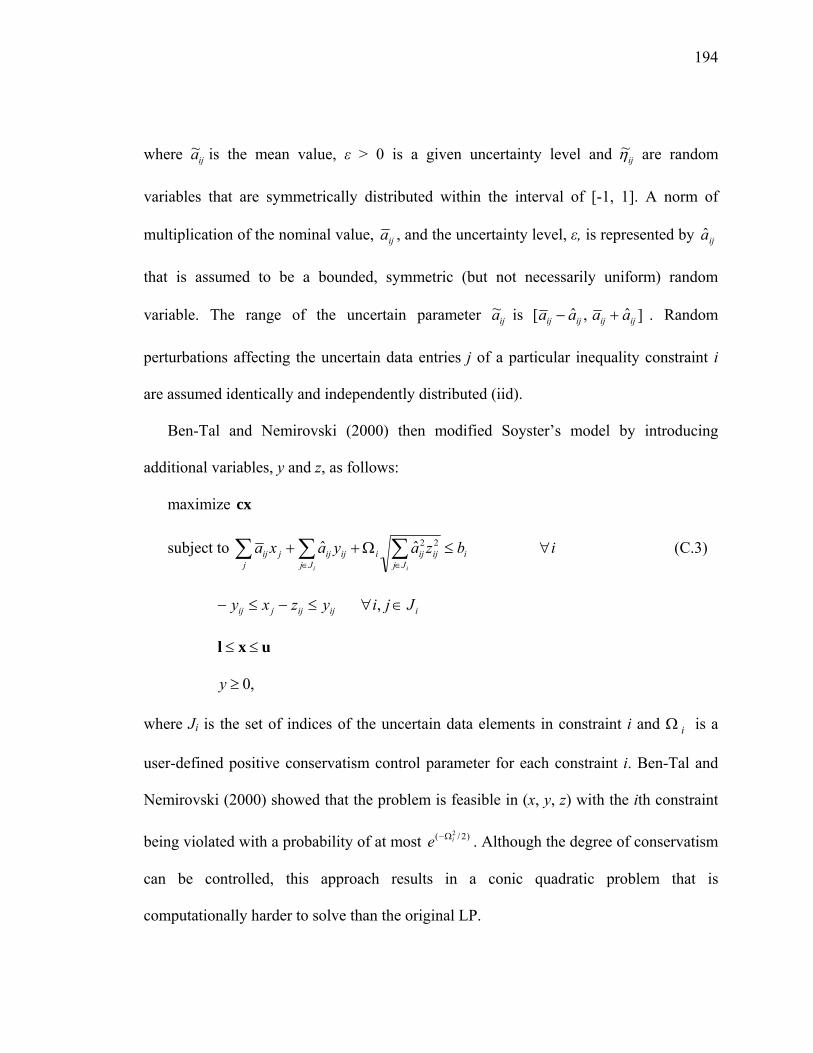
194
where ija~ is the mean value, ε > 0 is a given uncertainty level and ijη~ are random
variables that are symmetrically distributed within the interval of [-1, 1]. A norm of
multiplication of the nominal value, ija , and the uncertainty level, ε, is represented by ija
that is assumed to be a bounded, symmetric (but not necessarily uniform) random
variable. The range of the uncertain parameter ija~ is ]ˆ,ˆ[ ijijijij aaaa +− . Random
perturbations affecting the uncertain data entries j of a particular inequality constraint i
are assumed identically and independently distributed (iid).
Ben-Tal and Nemirovski (2000) then modified Soyster’s model by introducing
additional variables, y and z, as follows:
maximize cx
subject to ij Jj
ijijiJj
ijijjij bzayaxaii
≤Ω++∑ ∑∑∈∈
22ˆˆ i∀ (C.3)
ijijjij yzxy ≤−≤− iJji ∈∀ ,
uxl ≤≤
,0≥y
where Ji is the set of indices of the uncertain data elements in constraint i and Ω i is a
user-defined positive conservatism control parameter for each constraint i. Ben-Tal and
Nemirovski (2000) showed that the problem is feasible in (x, y, z) with the ith constraint
being violated with a probability of at most )2/( 2ie Ω− . Although the degree of conservatism
can be controlled, this approach results in a conic quadratic problem that is
computationally harder to solve than the original LP.
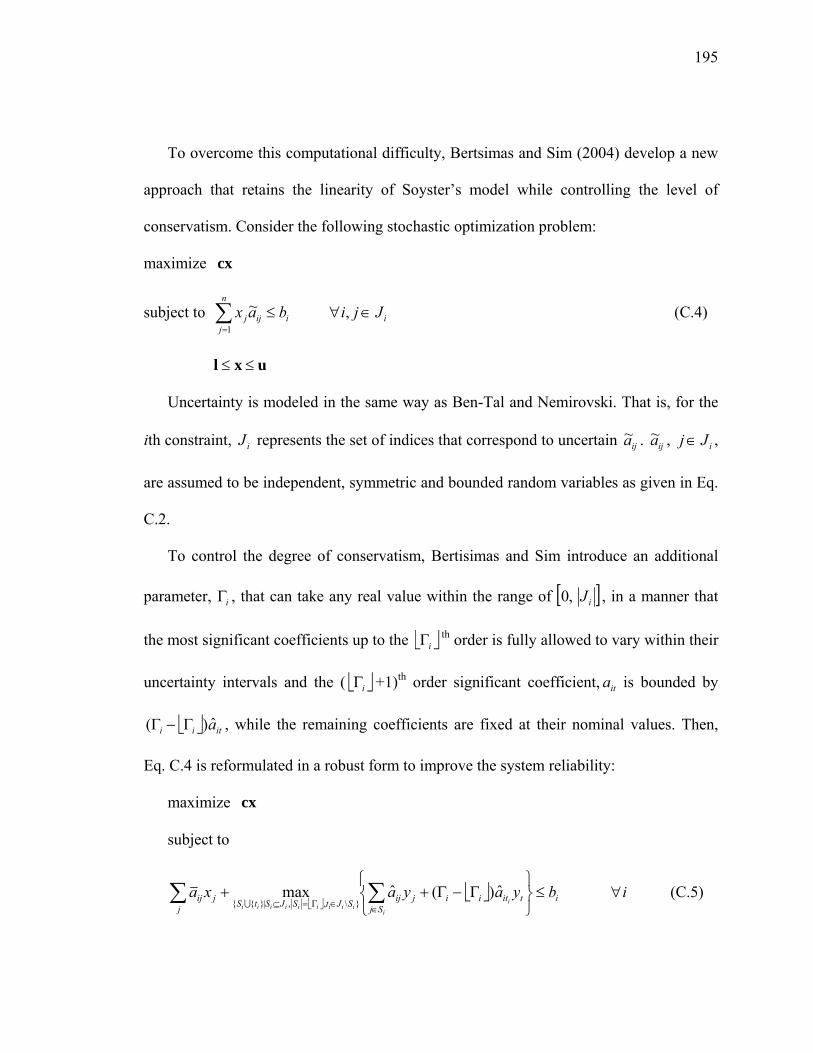
195
To overcome this computational difficulty, Bertsimas and Sim (2004) develop a new
approach that retains the linearity of Soyster’s model while controlling the level of
conservatism. Consider the following stochastic optimization problem:
maximize cx
subject to i
n
jijj bax ≤∑
=1
~ iJji ∈∀ , (C.4)
uxl ≤≤
Uncertainty is modeled in the same way as Ben-Tal and Nemirovski. That is, for the
ith constraint, iJ represents the set of indices that correspond to uncertain ija~ . ija~ , iJj ∈ ,
are assumed to be independent, symmetric and bounded random variables as given in Eq.
C.2.
To control the degree of conservatism, Bertisimas and Sim introduce an additional
parameter, iΓ , that can take any real value within the range of [ ]iJ,0 , in a manner that
the most significant coefficients up to the ⎣ ⎦iΓ th order is fully allowed to vary within their
uncertainty intervals and the ( ⎣ ⎦iΓ +1)th order significant coefficient, ita is bounded by
⎣ ⎦ itii a)( Γ−Γ , while the remaining coefficients are fixed at their nominal values. Then,
Eq. C.4 is reformulated in a robust form to improve the system reliability:
maximize cx
subject to
⎣ ⎦⎣ ⎦ ititii
SjjijSJtSJStSj
jij byayaxa
i
iiiiiiiiii
≤⎭⎬⎫
⎩⎨⎧
Γ−Γ++ ∑∑∈∈Γ=⊆
ˆ)(ˆmax\,,| U
i∀ (C.5)
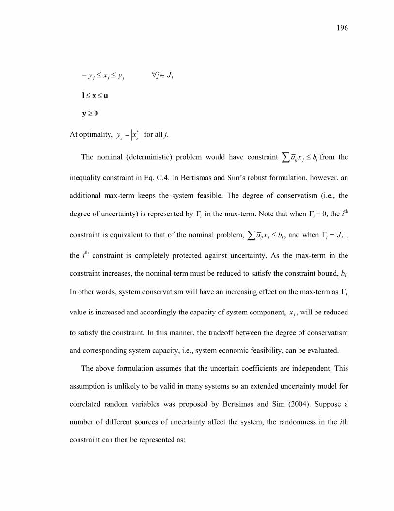
196
jjj yxy ≤≤− iJj ∈∀
uxl ≤≤
0y ≥
At optimality, *jj xy = for all j.
The nominal (deterministic) problem would have constraint ijij bxa ≤∑ from the
inequality constraint in Eq. C.4. In Bertismas and Sim’s robust formulation, however, an
additional max-term keeps the system feasible. The degree of conservatism (i.e., the
degree of uncertainty) is represented by iΓ in the max-term. Note that when iΓ = 0, the ith
constraint is equivalent to that of the nominal problem, ijij bxa ≤∑ , and when ii J=Γ ,
the ith constraint is completely protected against uncertainty. As the max-term in the
constraint increases, the nominal-term must be reduced to satisfy the constraint bound, bi.
In other words, system conservatism will have an increasing effect on the max-term as iΓ
value is increased and accordingly the capacity of system component, jx , will be reduced
to satisfy the constraint. In this manner, the tradeoff between the degree of conservatism
and corresponding system capacity, i.e., system economic feasibility, can be evaluated.
The above formulation assumes that the uncertain coefficients are independent. This
assumption is unlikely to be valid in many systems so an extended uncertainty model for
correlated random variables was proposed by Bertsimas and Sim (2004). Suppose a
number of different sources of uncertainty affect the system, the randomness in the ith
constraint can then be represented as:
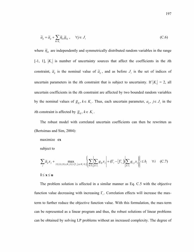
197
∑∈
+=iKk
kjikijij gaa η~~ , iJj ∈∀ (C.6)
where ikη~ are independently and symmetrically distributed random variables in the range
[-1, 1], iK is number of uncertainty sources that affect the coefficients in the ith
constraint, ija is the nominal value of ija~ , and as before iJ is the set of indices of
uncertain parameters in the ith constraint that is subject to uncertainty. If iK = 2, all
uncertain coefficients in the ith constraint are affected by two bounded random variables
by the nominal values of ikj Kkg ∈, . Thus, each uncertain parameter, iij Jja ∈, in the
ith constraint is affected by ikj Kkg ∈, .
The robust model with correlated uncertain coefficients can then be rewritten as
(Bertsimas and Sim, 2004):
maximize cx
subject to
⎣ ⎦⎣ ⎦ i
Jjjjtii
Sk JjjkjSKtSKStSj
jij bxgxgxa
i
i
i iiiiiiiiii
≤⎪⎭
⎪⎬⎫
⎪⎩
⎪⎨⎧
Γ−Γ++ ∑∑ ∑∑∈∈ ∈∈Γ=⊆
)(max\,,| U
i∀ (C.7)
uxl ≤≤
The problem solution is affected in a similar manner as Eq. C.5 with the objective
function value decreasing with increasing iΓ . Correlation effects will increase the max-
term to further reduce the objective function value. With this formulation, the max-term
can be represented as a linear program and thus, the robust solutions of linear problems
can be obtained by solving LP problems without an increased complexity. The degree of
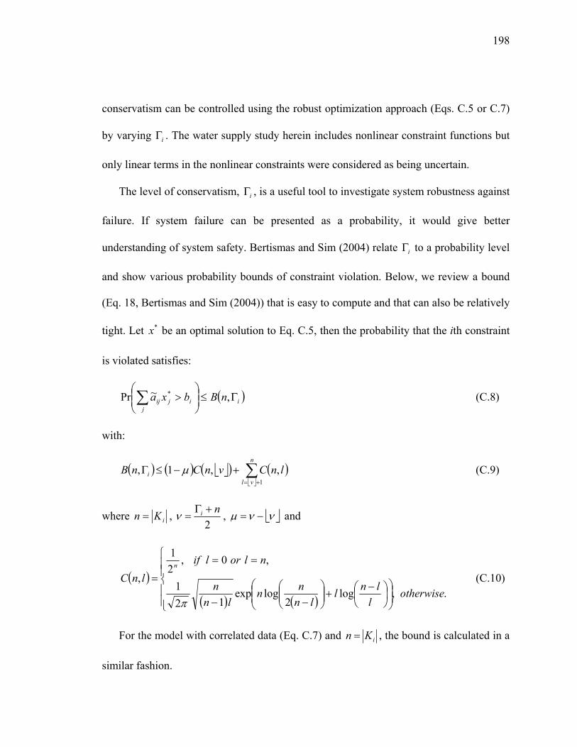
198
conservatism can be controlled using the robust optimization approach (Eqs. C.5 or C.7)
by varying iΓ . The water supply study herein includes nonlinear constraint functions but
only linear terms in the nonlinear constraints were considered as being uncertain.
The level of conservatism, iΓ , is a useful tool to investigate system robustness against
failure. If system failure can be presented as a probability, it would give better
understanding of system safety. Bertismas and Sim (2004) relate iΓ to a probability level
and show various probability bounds of constraint violation. Below, we review a bound
(Eq. 18, Bertismas and Sim (2004)) that is easy to compute and that can also be relatively
tight. Let *x be an optimal solution to Eq. C.5, then the probability that the ith constraint
is violated satisfies:
( )iijj
ij nBbxa Γ≤⎟⎟⎠
⎞⎜⎜⎝
⎛>∑ ,~Pr * (C.8)
with:
( ) ( ) ⎣ ⎦( ) ( )⎣ ⎦∑
+=
+−≤Γn
vli lnCvnCnB
1
,,1, µ (C.9)
where iKn = , 2
ni +Γ=ν , ⎣ ⎦ννµ −= and
( )
( ) ( )⎪⎪⎩
⎪⎪⎨
⎧
⎟⎟⎠
⎞⎜⎜⎝
⎛⎟⎠⎞
⎜⎝⎛ −
+⎟⎟⎠
⎞⎜⎜⎝
⎛−−
==
=.,log
2logexp
121
,0,21
,otherwise
llnl
lnnn
lnn
nlorliflnC
n
π
(C.10)
For the model with correlated data (Eq. C.7) and iKn = , the bound is calculated in a
similar fashion.
199
To compute iΓ values, the probability level in Eq. C.8 and ( )inB Γ, is defined for
each of the i uncertain constraints. Assuming Eq. C.9 is tight, iΓ can be directly
computed using Eq. C.10. Each uncertain constraint is considered independently to
determine its corresponding iΓ . With the set of iΓ , the optimal solution for the defined
probability level is determined by solving problem C.5 or C.7. A range of probability
levels can be evaluated to provide the decision maker the tradeoff between robustness
and cost.
3. APPLICATION TO WATER SUPPLY SYSTEM
3.1 Problem Statement
The robust optimization methodology is applied to a realistic hypothetical water
supply system (Figure C.1). The problem objective is to minimize the total cost for the
construction, expansion, and operation of the system. The appendix includes a complete
list of indices, sets, input parameters, and variables. To model the water supply system,
we have a graph G = (N, A), where N is the set of nodes and A is the set of arcs (Figure
C.1). N consists of 8 nodes: sources (NS - imported water, aquifer, upstream river, and
downstream river), users (NU - domestic and irrigation), and water and wastewater
treatment plants (NWT and NWWT, respectively). Note a river is represented by upstream
(NRU) and downstream (NRD) nodes and a connecting arc. Sources are divided into two
subsets: storage sources (NSS) and non-storage sources (NNS) depending on the capability
200
of storing water from the previous time step. For instance, a groundwater aquifer is a
storage source while imported water and upstream and downstream rivers are non-storage
sources.
The system can be constructed or expanded in year t and operational time is
represented by o. T and O are the set of construction/expansion and operational times. A
15-year planning period is evaluated and new facilities may only be constructed in years
1 and 6. Existing infrastructure is in place at year 0. Operation variables ( oijq ) over arcs (i,
j) during each operation period, o, are determined each year ( 1=∆o ) for the first 5 years
(first design period) and every other year ( 2=∆o ) for the last 10 years (second design
period).
In out model, A consists of 18 arcs (i, j) that connects nodes i and j. Arcs represent
canals (AC − arcs 1, 2, 3, 4 and 5 in Figure C.1), pipe lines (AP −arcs 8, 9, 10 and 11),
pump stations (AU − arcs 6 and 7), rainfall or mountain frontal recharge (AR – arcs 12, 13,
14 and 15), and seepage or infiltration (AI – arcs 16, 17 and 18). Pump stations are
located in arcs to overcome friction losses and elevation differences through pipe
connections. To permit water banking, arc 4 represents a canal to carry imported water to
recharge basins.
Before providing the mathematical model details, an overview of model equations is
presented in verbal terms. The objective function and system constraints are:
Minimize
)(1tijf κ - construction cost of pipe arcs (i, j) in expansion year t
201
+ )(2tijdf - construction cost of canal arcs (i, j) in expansion year t
+ ),(3tij
tij Hf χ - construction cost of pump on arcs (i, j) in expansion year t
+ )(4tiwf - construction cost of treatment plant i in expansion year t
+ ),(5oi
oij wqf - operation and maintenance cost of the system in operation year o
+ )(6oIWf - water purchased cost from outside of basin in operation year o
Subject to
1 Meet water demand for water users (domestic and agricultural area)
2 Do not exceed water and wastewater treatment plant capacity
3 Restrict the amount of imported water to the external water availability
4 Satisfy conservation of mass in non-storage nodes, users, and treatment plants.
5 Meet required river discharge at downstream river node
6 Meet required groundwater storage to maintain a sustainable system
7 Satisfy conservation of mass in storage nodes
8 Limit canal flow by maximum canal capacity
9 Maintain pump operating efficiency
10 Meet minimum pressure requirement at the end of pipe arcs
11 Meet minimum pressure requirement at the end of pump arcs
Design decisions are the arc or node capacities, such as pipe sizes, pump design head
and flow rate, canal depth, and water and wastewater treatment plant capacities. Flow
allocations over the water supply network are operational control variables.
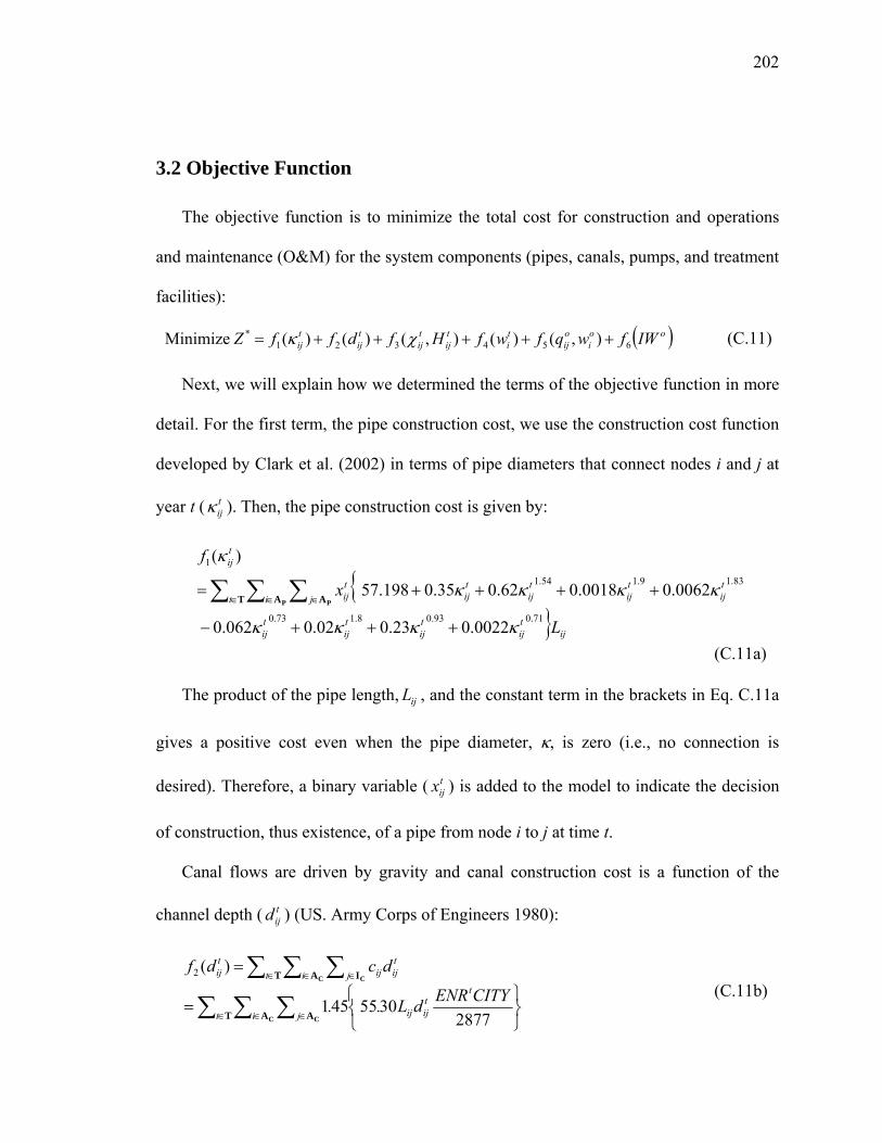
202
3.2 Objective Function
The objective function is to minimize the total cost for construction and operations
and maintenance (O&M) for the system components (pipes, canals, pumps, and treatment
facilities):
( )ooi
oij
ti
tij
tij
tij
tij IWfwqfwfHfdffZ 654321
* ),()(),()()(Minimize +++++= χκ (C.11)
Next, we will explain how we determined the terms of the objective function in more
detail. For the first term, the pipe construction cost, we use the construction cost function
developed by Clark et al. (2002) in terms of pipe diameters that connect nodes i and j at
year t ( tijκ ). Then, the pipe construction cost is given by:
ij
tij
tij
tij
tij
t i jtij
tij
tij
tij
tij
tij
L
x
f
71.093.08.173.0
83.19.154.1
1
0022.023.002.0062.0
0062.00018.062.035.0198.57
)(
κκκκ
κκκκ
κ
+++−
++++= ∑ ∑ ∑∈ ∈ ∈T A AP P
(C.11a)
The product of the pipe length, ijL , and the constant term in the brackets in Eq. C.11a
gives a positive cost even when the pipe diameter, κ, is zero (i.e., no connection is
desired). Therefore, a binary variable ( tijx ) is added to the model to indicate the decision
of construction, thus existence, of a pipe from node i to j at time t.
Canal flows are driven by gravity and canal construction cost is a function of the
channel depth ( tijd ) (US. Army Corps of Engineers 1980):
∑ ∑ ∑
∑ ∑ ∑
∈ ∈ ∈
∈ ∈ ∈
⎭⎬⎫
⎩⎨⎧
=
=
T A A
T A I
C C
C C
t i j
ttijij
t i jtijij
tij
CITYENRdL..
dcdf
28773055451
)(2
(C.11b)
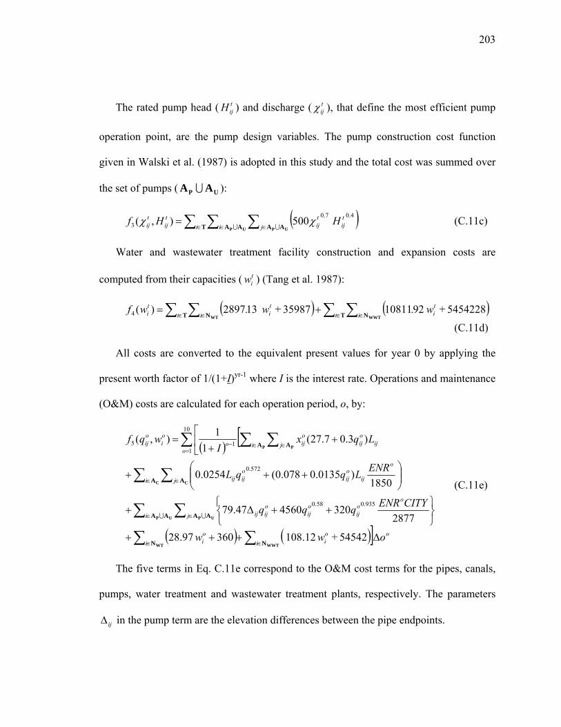
203
The rated pump head ( tijH ) and discharge ( t
ijχ ), that define the most efficient pump
operation point, are the pump design variables. The pump construction cost function
given in Walski et al. (1987) is adopted in this study and the total cost was summed over
the set of pumps ( UP AA U ):
( )∑ ∑ ∑∈ ∈ ∈=
T AA AAUP UPt i jtij
tij
tij
tij HHf
U U
4.07.03 500),( χχ (C.11c)
Water and wastewater treatment facility construction and expansion costs are
computed from their capacities ( tiw ) (Tang et al. 1987):
( ) ( )∑ ∑∑ ∑ ∈ ∈∈ ∈+=
T NT N WWTWT t itit i
ti
ti w.w.wf 5454228 + 921081135987 + 132897)(4
(C.11d)
All costs are converted to the equivalent present values for year 0 by applying the
present worth factor of 1/(1+I)yr-1 where I is the interest rate. Operations and maintenance
(O&M) costs are calculated for each operation period, o, by:
( )[
( ) ( )] oi
oii
oi
i j
ooij
oij
oijij
i j
o
ijoij
oijij
oi j ij
oij
oijo
oi
oij
oww
CITYENRqqq
ENRLqqL
LqxI
wqf
∆+++⎭⎬⎫
⎩⎨⎧
++∆+
⎟⎟⎠
⎞⎜⎜⎝
⎛+++
⎢⎣
⎡+
+=
∑∑
∑ ∑
∑ ∑
∑ ∑ ∑
∈∈
∈ ∈
∈ ∈
=∈ ∈−
WWTWT
UP UP
C C
P P
NN
AA AA
A A
A A
54542 + 108.12 36097.28
2877320456047.79
1850)0135.0078.0(0254.0
)3.07.27(1
1),(
935.058.0
572.0
10
115
U U
(C.11e)
The five terms in Eq. C.11e correspond to the O&M cost terms for the pipes, canals,
pumps, water treatment and wastewater treatment plants, respectively. The parameters
ij∆ in the pump term are the elevation differences between the pipe endpoints.
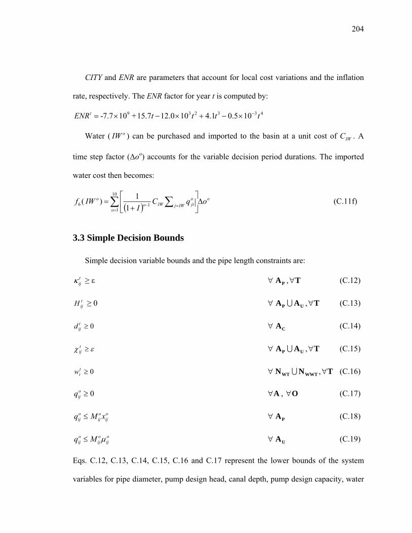
204
CITY and ENR are parameters that account for local cost variations and the inflation
rate, respectively. The ENR factor for year t is computed by:
105.01.4100.127.15 +10.77- 433239 ttttENRt −×−+×−×=
Water ( oIW ) can be purchased and imported to the basin at a unit cost of IWC . A
time step factor (∆oo) accounts for the variable decision period durations. The imported
water cost then becomes:
( )o
oIWj
ojiIWo
o oqCI
IWf ∆⎥⎦
⎤⎢⎣
⎡
+= ∑ ∑
==−
10
116 1
1)( (C.11f)
3.3 Simple Decision Bounds
Simple decision variable bounds and the pipe length constraints are:
tijκ ≥ ε PA∀ , T∀ (C.12)
tijH ≥ 0 UP AA U∀ , T∀ (C.13)
0≥tijd CA∀ (C.14)
εχ ≥tij UP AA U∀ , T∀ (C.15)
0≥tiw WWTWT NN U∀ , T∀ (C.16)
0≥oijq A∀ , O∀ (C.17)
oij
oij
oij xMq ≤ PA∀ (C.18)
oij
oij
oij Mq µ≤ UA∀ (C.19)
Eqs. C.12, C.13, C.14, C.15, C.16 and C.17 represent the lower bounds of the system
variables for pipe diameter, pump design head, canal depth, pump design capacity, water
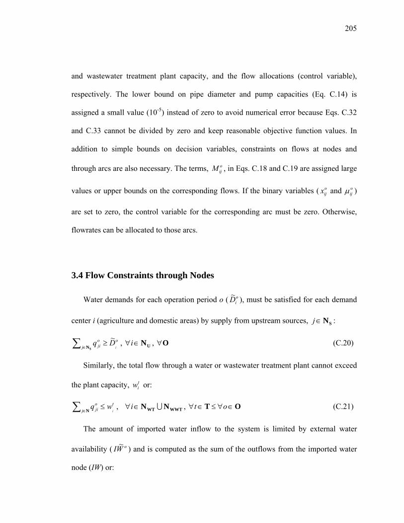
205
and wastewater treatment plant capacity, and the flow allocations (control variable),
respectively. The lower bound on pipe diameter and pump capacities (Eq. C.14) is
assigned a small value (10-5) instead of zero to avoid numerical error because Eqs. C.32
and C.33 cannot be divided by zero and keep reasonable objective function values. In
addition to simple bounds on decision variables, constraints on flows at nodes and
through arcs are also necessary. The terms, oijM , in Eqs. C.18 and C.19 are assigned large
values or upper bounds on the corresponding flows. If the binary variables ( oijx and o
ijµ )
are set to zero, the control variable for the corresponding arc must be zero. Otherwise,
flowrates can be allocated to those arcs.
3.4 Flow Constraints through Nodes
Water demands for each operation period o ( oiD~ ), must be satisfied for each demand
center i (agriculture and domestic areas) by supply from upstream sources, SN∈j :
∑ ∈≥
SNjoo
ji iDq ~ , UN∈∀i , O∀ (C.20)
Similarly, the total flow through a water or wastewater treatment plant cannot exceed
the plant capacity, tiw or:
∑ ∈≤
Njto
ji iwq , WWTWT NN U∈∀i , OT ∈∀≤∈∀ ot (C.21)
The amount of imported water inflow to the system is limited by external water
availability ( oWI ~ ) and is computed as the sum of the outflows from the imported water
node (IW) or:
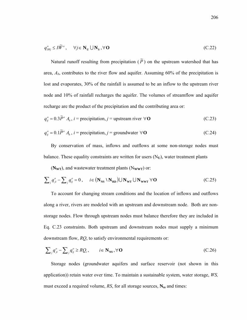
206
ooIWj WIq ~≤ , SU NN U∈∀j , O∀ (C.22)
Natural runoff resulting from precipitation ( P~ ) on the upstream watershed that has
area, Ab, contributes to the river flow and aquifer. Assuming 60% of the precipitation is
lost and evaporates, 30% of the rainfall is assumed to be an inflow to the upstream river
node and 10% of rainfall recharges the aquifer. The volumes of streamflow and aquifer
recharge are the product of the precipitation and the contributing area or:
boo
ij APq ~3.0= , i = precipitation, j = upstream river O∀ (C.23)
boo
ij APq ~1.0= , i = precipitation, j = groundwater O∀ (C.24)
By conservation of mass, inflows and outflows at some non-storage nodes must
balance. These equality constraints are written for users (NU), water treatment plants
(NWT), and wastewater treatment plants (NWWT) or:
0=− ∑∑ joijj
oji qq , ( ) WWTWTRDNS NNN\N UU∈i O∀ (C.25)
To account for changing stream conditions and the location of inflows and outflows
along a river, rivers are modeled with an upstream and downstream node. Both are non-
storage nodes. Flow through upstream nodes must balance therefore they are included in
Eq. C.23 constraints. Both upstream and downstream nodes must supply a minimum
downstream flow, RQ, to satisfy environmental requirements or:
ijoijj
oji RQqq ≥− ∑∑ , NSN∈i , O∀ (C.26)
Storage nodes (groundwater aquifers and surface reservoir (not shown in this
application)) retain water over time. To maintain a sustainable system, water storage, WS,
must exceed a required volume, RS, for all storage sources, Nss and times:
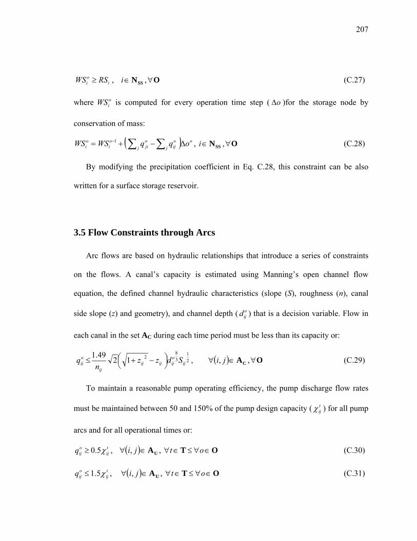
207
ioi RSWS ≥ , SSN∈i , O∀ (C.27)
where oiWS is computed for every operation time step ( o∆ )for the storage node by
conservation of mass:
( ) oj
oijj
oji
oi
oi oqqWSWS ∆−+= ∑∑−1 , SSN∈i , O∀ (C.28)
By modifying the precipitation coefficient in Eq. C.28, this constraint can be also
written for a surface storage reservoir.
3.5 Flow Constraints through Arcs
Arc flows are based on hydraulic relationships that introduce a series of constraints
on the flows. A canal’s capacity is estimated using Manning’s open channel flow
equation, the defined channel hydraulic characteristics (slope (S), roughness (n), canal
side slope (z) and geometry), and channel depth ( oijd ) that is a decision variable. Flow in
each canal in the set AC during each time period must be less than its capacity or:
21
38
21249.1ij
oijijij
ij
oij Sdzz
nq ⎟
⎠⎞⎜
⎝⎛ −+≤ , ( ) CA∈∀ ji, , O∀ (C.29)
To maintain a reasonable pump operating efficiency, the pump discharge flow rates
must be maintained between 50 and 150% of the pump design capacity ( tijχ ) for all pump
arcs and for all operational times or:
tij
oijq χ5.0≥ , ( ) UA∈∀ ji, , OT ∈∀≤∈∀ ot (C.30)
tij
oijq χ5.1≤ , ( ) UA∈∀ ji, , OT ∈∀≤∈∀ ot (C.31)
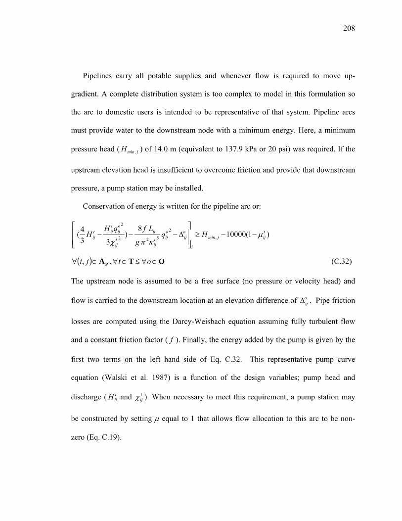
208
Pipelines carry all potable supplies and whenever flow is required to move up-
gradient. A complete distribution system is too complex to model in this formulation so
the arc to domestic users is intended to be representative of that system. Pipeline arcs
must provide water to the downstream node with a minimum energy. Here, a minimum
pressure head ( jminH , ) of 14.0 m (equivalent to 137.9 kPa or 20 psi) was required. If the
upstream elevation head is insufficient to overcome friction and provide that downstream
pressure, a pump station may be installed.
Conservation of energy is written for the pipeline arc or:
( ) PA∈∀ ji, , OT ∈∀≤∈∀ ot (C.32)
The upstream node is assumed to be a free surface (no pressure or velocity head) and
flow is carried to the downstream location at an elevation difference of oij∆ . Pipe friction
losses are computed using the Darcy-Weisbach equation assuming fully turbulent flow
and a constant friction factor ( f ). Finally, the energy added by the pump is given by the
first two terms on the left hand side of Eq. C.32. This representative pump curve
equation (Walski et al. 1987) is a function of the design variables; pump head and
discharge ( tijH and t
ijχ ). When necessary to meet this requirement, a pump station may
be constructed by setting µ equal to 1 that allows flow allocation to this arc to be non-
zero (Eq. C.19).
)1(100008
)33
4( ,2
522
2tijjmin
i
oij
oijt
ij
ij
tij
oij
tijt
ij Hqg
LfqHH µ
κπχ−−≥
⎥⎥⎦
⎤
⎢⎢⎣
⎡∆−−−
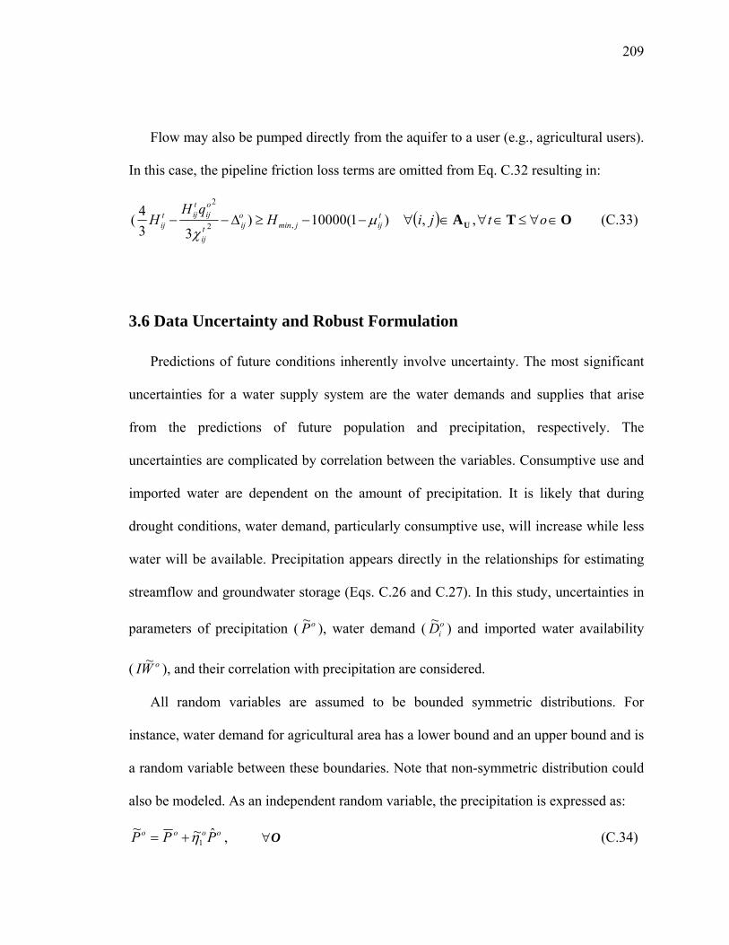
209
Flow may also be pumped directly from the aquifer to a user (e.g., agricultural users).
In this case, the pipeline friction loss terms are omitted from Eq. C.32 resulting in:
)1(10000)33
4( ,2
2tijjmin
oijt
ij
oij
tijt
ij HqH
H µχ
−−≥∆−− ( ) UA∈∀ ji, , OT ∈∀≤∈∀ ot (C.33)
3.6 Data Uncertainty and Robust Formulation
Predictions of future conditions inherently involve uncertainty. The most significant
uncertainties for a water supply system are the water demands and supplies that arise
from the predictions of future population and precipitation, respectively. The
uncertainties are complicated by correlation between the variables. Consumptive use and
imported water are dependent on the amount of precipitation. It is likely that during
drought conditions, water demand, particularly consumptive use, will increase while less
water will be available. Precipitation appears directly in the relationships for estimating
streamflow and groundwater storage (Eqs. C.26 and C.27). In this study, uncertainties in
parameters of precipitation ( oP~ ), water demand ( oiD~ ) and imported water availability
( oWI ~ ), and their correlation with precipitation are considered.
All random variables are assumed to be bounded symmetric distributions. For
instance, water demand for agricultural area has a lower bound and an upper bound and is
a random variable between these boundaries. Note that non-symmetric distribution could
also be modeled. As an independent random variable, the precipitation is expressed as:
oooo PPP ˆ~~1η+= , O∀ (C.34)
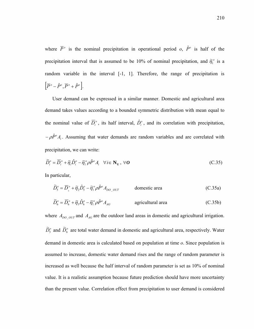
210
where oP is the nominal precipitation in operational period o, oP is half of the
precipitation interval that is assumed to be 10% of nominal precipitation, and o1
~η is a
random variable in the interval [-1, 1]. Therefore, the range of precipitation is
[ ]oooo PPPP ˆ,ˆ +− .
User demand can be expressed in a similar manner. Domestic and agricultural area
demand takes values according to a bounded symmetric distribution with mean equal to
the nominal value of oiD , its half interval, o
iD , and its correlation with precipitation,
io APρ− . Assuming that water demands are random variables and are correlated with
precipitation, we can write:
iooo
iio
ioi APDDD ˆ~ˆ~~
1 ρηη −+= UN∈∀i , O∀ (C.35)
In particular,
OUTDOooooo APDDD _1525
ˆ~ˆ~~5
ρηη −+= domestic area (C.35a)
AGooooo APDDD ˆ~ˆ~~
16366 ρηη −+= agricultural area (C.35b)
where OUTDOA _ and AGA are the outdoor land areas in domestic and agricultural irrigation.
oD5~ and oD6
~ are total water demand in domestic and agricultural area, respectively. Water
demand in domestic area is calculated based on population at time o. Since population is
assumed to increase, domestic water demand rises and the range of random parameter is
increased as well because the half interval of random parameter is set as 10% of nominal
value. It is a realistic assumption because future prediction should have more uncertainty
than the present value. Correlation effect from precipitation to user demand is considered
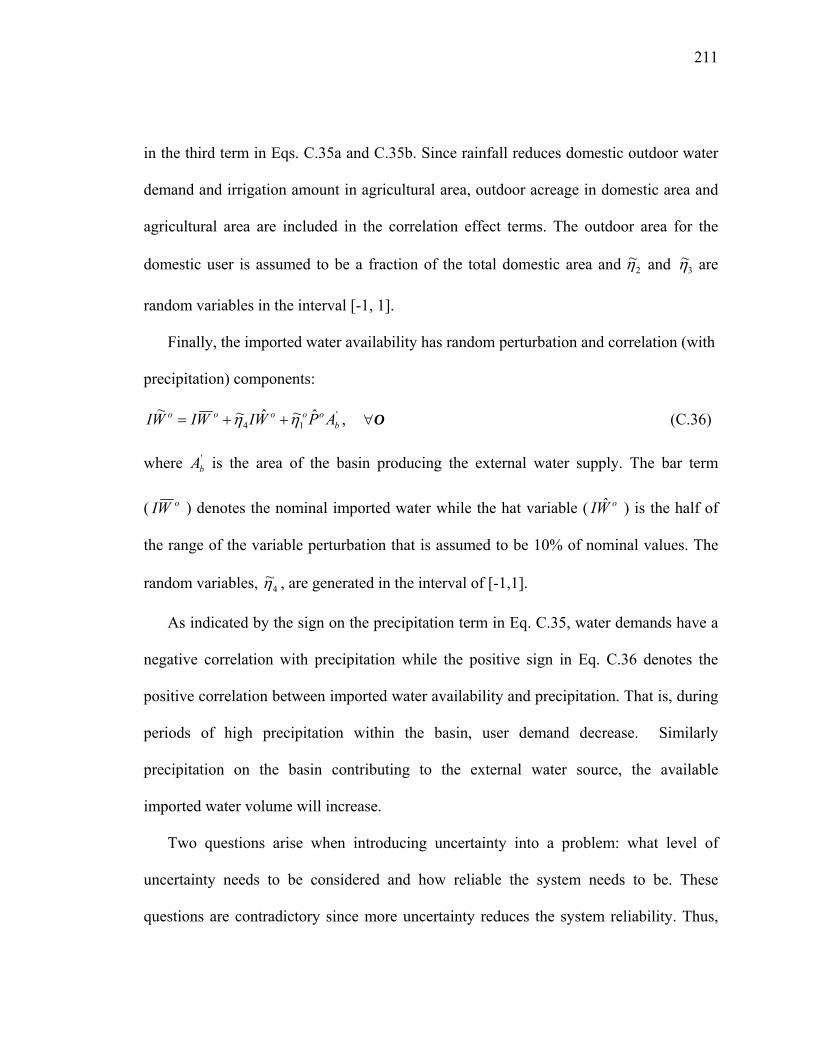
211
in the third term in Eqs. C.35a and C.35b. Since rainfall reduces domestic outdoor water
demand and irrigation amount in agricultural area, outdoor acreage in domestic area and
agricultural area are included in the correlation effect terms. The outdoor area for the
domestic user is assumed to be a fraction of the total domestic area and 2~η and 3
~η are
random variables in the interval [-1, 1].
Finally, the imported water availability has random perturbation and correlation (with
precipitation) components:
'14
ˆ~ˆ~~b
ooooo APWIWIWI ηη ++= , O∀ (C.36)
where 'bA is the area of the basin producing the external water supply. The bar term
( oWI ) denotes the nominal imported water while the hat variable ( oWI ˆ ) is the half of
the range of the variable perturbation that is assumed to be 10% of nominal values. The
random variables, 4~η , are generated in the interval of [-1,1].
As indicated by the sign on the precipitation term in Eq. C.35, water demands have a
negative correlation with precipitation while the positive sign in Eq. C.36 denotes the
positive correlation between imported water availability and precipitation. That is, during
periods of high precipitation within the basin, user demand decrease. Similarly
precipitation on the basin contributing to the external water source, the available
imported water volume will increase.
Two questions arise when introducing uncertainty into a problem: what level of
uncertainty needs to be considered and how reliable the system needs to be. These
questions are contradictory since more uncertainty reduces the system reliability. Thus,
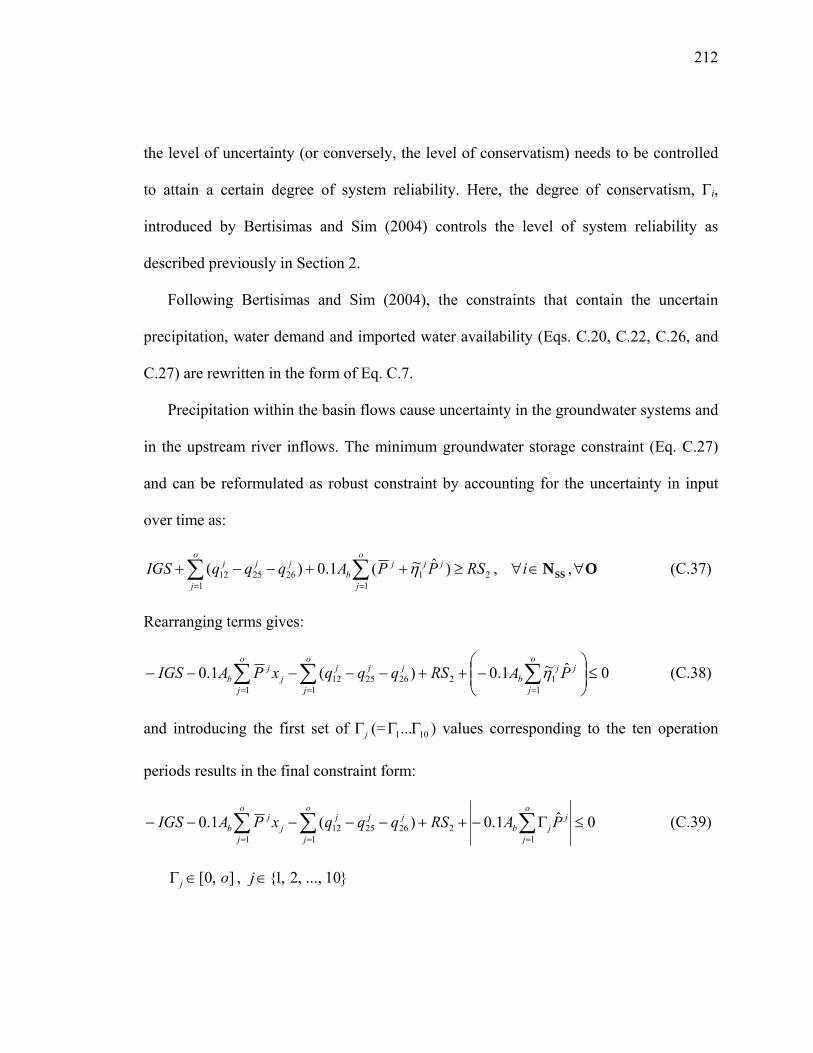
212
the level of uncertainty (or conversely, the level of conservatism) needs to be controlled
to attain a certain degree of system reliability. Here, the degree of conservatism, Γi,
introduced by Bertisimas and Sim (2004) controls the level of system reliability as
described previously in Section 2.
Following Bertisimas and Sim (2004), the constraints that contain the uncertain
precipitation, water demand and imported water availability (Eqs. C.20, C.22, C.26, and
C.27) are rewritten in the form of Eq. C.7.
Precipitation within the basin flows cause uncertainty in the groundwater systems and
in the upstream river inflows. The minimum groundwater storage constraint (Eq. C.27)
and can be reformulated as robust constraint by accounting for the uncertainty in input
over time as:
21
11
262512 )ˆ~(1.0)( RSPPAqqqIGSo
j
jjjb
o
j
jjj ≥++−−+ ∑∑==
η , SSN∈∀i , O∀ (C.37)
Rearranging terms gives:
0ˆ~1.0)(1.01
121
2625121
≤⎟⎟⎠
⎞⎜⎜⎝
⎛−++−−−−− ∑∑∑
===
o
j
jjb
o
j
jjjo
jj
jb PARSqqqxPAIGS η (C.38)
and introducing the first set of jΓ (= 101...ΓΓ ) values corresponding to the ten operation
periods results in the final constraint form:
0ˆ1.0)(1.01
21
2625121
≤Γ−++−−−−− ∑∑∑===
o
j
jjb
o
j
jjjo
jj
jb PARSqqqxPAIGS (C.39)
],0[ oj ∈Γ , 10...,,2,1∈j
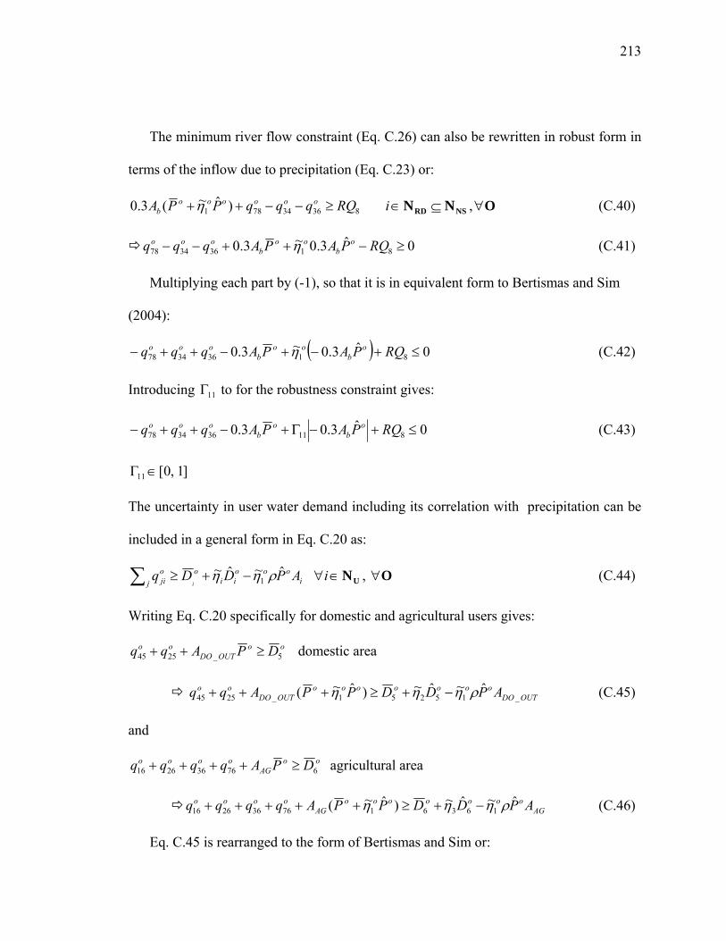
213
The minimum river flow constraint (Eq. C.26) can also be rewritten in robust form in
terms of the inflow due to precipitation (Eq. C.23) or:
83634781 )ˆ~(3.0 RQqqqPPA oooooob ≥−−++η NSRD NN ⊆∈i , O∀ (C.40)
0ˆ3.0~3.0 81363478 ≥−++−− RQPAPAqqq ob
oob
ooo η (C.41)
Multiplying each part by (-1), so that it is in equivalent form to Bertismas and Sim
(2004):
( ) 0ˆ3.0~3.0 81363478 ≤+−+−++− RQPAPAqqq ob
oob
ooo η (C.42)
Introducing 11Γ to for the robustness constraint gives:
0ˆ3.03.0 811363478 ≤+−Γ+−++− RQPAPAqqq ob
ob
ooo (C.43)
]1,0[11 ∈Γ
The uncertainty in user water demand including its correlation with precipitation can be
included in a general form in Eq. C.20 as:
iooo
iio
joji APDDq
iˆ~ˆ~
1 ρηη −+≥∑ UN∈∀i , O∀ (C.44)
Writing Eq. C.20 specifically for domestic and agricultural users gives:
ooOUTDO
oo DPAqq 5_2545 ≥++ domestic area
OUTDOooooooo
OUTDOoo APDDPPAqq _15251_2545
ˆ~ˆ~)ˆ~( ρηηη −+≥+++ (C.45)
and
ooAG
oooo DPAqqqq 676362616 ≥++++ agricultural area
AGooooooo
AGoooo APDDPPAqqqq ˆ~ˆ~)ˆ~( 1636176362616 ρηηη −+≥+++++ (C.46)
Eq. C.45 is rearranged to the form of Bertismas and Sim or:
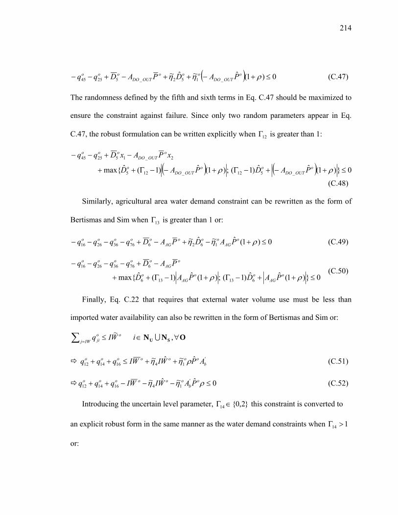
214
( ) 0)1(ˆ~ˆ~_152_52545 ≤+−++−+−− ρηη o
OUTDOooo
OUTDOooo PADPADqq (C.47)
The randomness defined by the fifth and sixth terms in Eq. C.47 should be maximized to
ensure the constraint against failure. Since only two random parameters appear in Eq.
C.47, the robust formulation can be written explicitly when 12Γ is greater than 1:
( ) ( ) 0)1(ˆˆ)1(;)1(ˆ)1(ˆmax _512_125
2_152545
≤+−+−Γ+−−Γ++
−+−−
ρρ oOUTDO
ooOUTDO
o
oOUTDO
ooo
PADPAD
xPAxDqq
(C.48)
Similarly, agricultural area water demand constraint can be rewritten as the form of
Bertismas and Sim when 13Γ is greater than 1 or:
0)1(ˆ~ˆ~162676362616 ≤+−+−+−−−− ρηη o
AGooo
AGooooo PADPADqqqq (C.49)
0)1(ˆˆ)1(;)1(ˆ)1(ˆmax 613136
676362616
≤++−Γ+−Γ++
−+−−−−
ρρ oAG
ooAG
o
oAG
ooooo
PADPAD
PADqqqq (C.50)
Finally, Eq. C.22 that requires that external water volume use must be less than
imported water availability can also be rewritten in the form of Bertismas and Sim or:
oIWj
oji WIq ~≤∑ =
SU NN U∈i , O∀
'14161412
ˆ~ˆ~b
ooooooo APWIWIqqq ρηη ++≤++ (C.51)
0ˆ~ˆ~ '14161412 ≤−−−++ ρηη o
boooooo PAWIWIqqq (C.52)
Introducing the uncertain level parameter, 2,014 ∈Γ this constraint is converted to
an explicit robust form in the same manner as the water demand constraints when 114 >Γ
or:
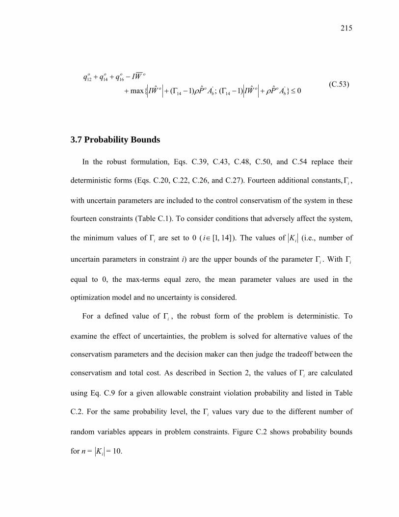
215
0ˆˆ)1(;ˆ)1(ˆmax '14
'14
161412
≤+−Γ−Γ++
−++
boo
boo
oooo
APWIAPWI
WIqqq
ρρ (C.53)
3.7 Probability Bounds
In the robust formulation, Eqs. C.39, C.43, C.48, C.50, and C.54 replace their
deterministic forms (Eqs. C.20, C.22, C.26, and C.27). Fourteen additional constants, iΓ ,
with uncertain parameters are included to the control conservatism of the system in these
fourteen constraints (Table C.1). To consider conditions that adversely affect the system,
the minimum values of iΓ are set to 0 ( ]14,1[∈i ). The values of iK (i.e., number of
uncertain parameters in constraint i) are the upper bounds of the parameter iΓ . With iΓ
equal to 0, the max-terms equal zero, the mean parameter values are used in the
optimization model and no uncertainty is considered.
For a defined value of iΓ , the robust form of the problem is deterministic. To
examine the effect of uncertainties, the problem is solved for alternative values of the
conservatism parameters and the decision maker can then judge the tradeoff between the
conservatism and total cost. As described in Section 2, the values of iΓ are calculated
using Eq. C.9 for a given allowable constraint violation probability and listed in Table
C.2. For the same probability level, the iΓ values vary due to the different number of
random variables appears in problem constraints. Figure C.2 shows probability bounds
for n = iK = 10.
216
4. RESULTS AND DISCUSSION
In some semi-arid regions, wastewater effluent is discharged to a normally dry or low
flow channel. Over time, a downstream riparian habitat develops that the effluent flow
sustains. If communities move to using reclaimed wastewater effluent for nonpotable and,
potentially, potable uses, this water would no longer be released to the riparian area. Thus,
communities face depletion of both surface and subsurface water sources and the decision
to maintain environmental flows.
The hypothetical community posed here requires developing new water supply
structures and sources while preserving environmental flow in the river stream and to the
aquifer. An external water source can be imported at a cost per unit volume plus the cost
of the conveyance to transport the water to the community.
The robust optimization method was applied to minimize the total cost of
construction, expansion, and operations and maintenance of a hypothetical water supply
system. The system includes subsurface (aquifer), surface, and imported water sources,
domestic and agricultural irrigation users, and water and wastewater treatment plants.
Input parameters for the system, nodes, and arcs are summarized in Tables C.3, C.4, and
C.5, respectively. As described above, a 15 year planning period that was divided into
two design periods and 10 operation periods was considered. Available water supply
system is listed in Table C.6. Figure C.3 shows flows and water supply structures at year
0. Groundwater is the main source to supply water demand of domestic and agricultural
217
areas at year 0. As the result, groundwater is depleted and water sustainability becomes
an issue in the hypothetical community. Groundwater storage at year 0 is 9.50 km3 that is
below the defined minimum storage of 9.93 km3. The optimized water supply plan must
increase groundwater storage to 9.93 km3 in the next fifteen years. To ensure riparian
health in this application, a minimum downstream river flow requirement is defined as
11.4 m3/s.
The water system’s arcs consist of five canals, four pipelines, and two pump stations.
The associated design decision at each design epoch are the canal depths, d, (5 canals),
pipe diameters, κ, (4 pipelines), pump design discharges, χ, (4 pump/pipelines + 2
pumps), pump design heads, H, (4 pump/pipelines + 2 pumps), and water and wastewater
treatment plant capacities, w, (2 plants). Thus, the total number of design decision
variables is 46 (23 × 2 design periods). In addition, the flows on 11 independent arcs
must be determined for each of the 10 operation periods. Lastly, the number of binary
variables for pipe flowrate, x, (4 pipelines × 10 operation periods) and pump flowrate, µ,
(4 pump/pipelines + 2 pumps) × 10 operation periods is 100. Thus, the optimization
problem contains a total number of 256 decision variables including 100 binary variables.
The continuous mixed-integer nonlinear problem were solved using GAMS/BARON
global optimization solver with the relative termination tolerance of 0.05 (Sahinidis and
Tawarmalani, 2005).
To demonstrate the overall formulation, this system is optimized for violation
probabilities ranging from 0.1 (the most conservative) to 1.0 (nominal). Figures C.4 and
C.5 show flows and design variables at year 1 in nominal (i.e., all Γ = 0) and robust
218
problems (P = 0.1). When constraint violation probability equals 0.1, the solution ensures
that all of the constraints remain feasible at least 90% of the time. The set of fourteen Γi
in this case (P = 0.1) is 1.00, 2.00, 3.00, 3.72, 4.20, 4.34, 4.61, 4.91, 4.93, 5.29, 1.00,
2.00, 2.00, 2.00 (Table C.2).
Groundwater storage requirement constraints (Eq. C. 39) have more uncertain
parameters ( iK ) in later operation periods. Uncertainty in yearly precipitation is
generated independently and total uncertainty increases over time. Domestic demands
increase with larger populations (Table C.12).
Optimal arc flows for the nominal and robust problems are listed in Tables C.7 and
C.8, respectively. Most noticeably, to meet the water demands imported water at year 1 in
the nominal problem (7.17 m3/s) is increased to 10.02 m3/s when P = 0.1. Due to the
expense of imported water ($0.81/m3), both alternatives replenish the aquifer with that
source in year 1 and no additional imported water is purchased. Both cases use reclaimed
water from wastewater treatment plant as the primary agricultural purpose. The robust
solution requires other sources while the nominal solution only uses a small amount
beyond reclaimed water.
Tables C.9 and C.10 lists the optimal design decisions for the two problems.
Domestic area demand increases over time as the population grows while agricultural
demand decreases after the 5th operation year. Therefore, few components are expanded
in the second design epoch (year 5). Capacities and heads of pumps that provide water
to and from domestic areas are expanded in nominal condition to meet the higher demand.
Increased domestic demand is supplied from the upstream river through the water
219
treatment plant that reduces water supply to the agricultural area from the upstream river.
Reclaimed water from wastewater treatment plant replaces this flow after year 5 and
requires the pump capacity to be expanded (Table C.9).
When the constraint violation probability is 0.1, only the pump capacity from
wastewater treatment plant to agricultural area is expanded; from 5.78 m3/s to 7.46 m3/s
because of increasing uncertainty in precipitation (Table C.10). Table C.11 lists
capacities of water and wastewater treatment plants in nominal problem and when
constraint violation probability is 0.1. A smaller water treatment plant is constructed in
the robust solution because supplying water to the domestic area from the aquifer is more
economical than expanding the water treatment plant. In this case, the aquifer is
recharged with imported water. The wastewater treatment plant capacity, however,
increases when constraint violation probability is 0.1 because effluent from domestic area
increases as demand rises.
As seen in Figure C.6, the optimal total cost depends upon the degree of
conservatism. As conservatism is raised (and constraint violation probability is
decreased), the total cost increases to insure system reliability by enlarging components
sizes or purchasing more imported water. In particular, the cost increases dramatically
between constraint violation probabilities of 0.7 and 0.5. At lower allowable constraint
violation probabilities, the cost is relatively flat. Up to about P = 0.5, the existing
expanded water treatment plant supplies water to domestic users. The flatness of the
curve demonstrates the economies of scale in meeting needs through the treatment
facility.
220
As the robustness requirement is increased, the strategy to meet demands changes.
The water treatment plant is not expanded rather its capacity remains at the initial size
(Table C.11). Given the demand, developing or expanding the conveyance system (canal
and pumping system) to import water and deliver it to domestic users becomes viable. As
seen in Figure C.7, the amount of imported water parallels the increase in cost. Above
the level of P=0.7, economies of scale again dominate and the incremental cost and
supply result in a relatively flat response.
5. CONCLUSIONS
In this study, a robust optimization approach was applied in a hypothetical water
supply system to minimize the total system cost. Considering that data in real systems
inherently involve uncertainties, it is important to consider these uncertainties during the
design process to improve the system reliability and robustness. This study found that the
robust optimization approach of Bertsimas and Sim could be a useful tool in the design of
water supply systems without introducing additional complexity into the optimization
problem.
Uncertainty was considered in water demand, water availability, and correlations
from precipitation to water demand and water availability, 14 of iΓ parameters were
added to the model, the probability of violating a constraint was related to those
parameters, and the problem was solved for a range of iΓ . The result was an NLP similar
in structure to the original NLP.
221
The hypothetical water supply system included subsurface, surface, imported water
sources, domestic and agricultural irrigational users, and water and wastewater treatment
plants as the system components. Initially, the system has available infrastructure that
was built to primarily provide water from surface and subsurface water sources.
Overall 15 years of the planning period was applied for the system evaluation. Two
design periods and 10 operation periods were evaluated to determine the values of total
256 decision variables with 100 binary decision variables. The problem was solved using
the GAMS/BARON software by a mixed branch and bound – (which NLP method)
method.
The effects of the degree of conservatism and the available water supply on total
system cost are investigated using probability bounds. Probability bounds are tied the
constraint violation as at most the probability of violation. From nominal problem to
conservative case (probability of violation is 0.1), optimal total costs are calculated and
the solutions are compared.
Water demand is driven by population growth rate, only a few expansion of structure
is suggested as an economic solution. Because of high cost to purchasing imported water,
external water source is introduced once at year 1 and recharges aquifer. Compared to the
nominal solution, conservative solutions import more water to maintain system reliability
and preserve environmental flows. As the result, total construction and operation cost
increase in the reliable water supply design. Given the small application system, water
treatment plant exits at year 0, expansion of the treatment plant is cheaper than building
other transportation facility to supply domestic area. After probability of constraint
222
violation is 0.5, economic solution is to construct larger canal and pumping station to
supply domestic demand. In this transaction period, total cost increases rapidly due to the
construction and importing water, then become relatively slow after then. The higher cost,
thus, is largely attributed to external water purchases.
Future work should move toward better representing the decisions including
discretized variables for pipe diameters and adding additional uncertain parameters, such
as temporal correlation over the operational time span. Also, adding more system
components such as commercial and industrial areas, public outdoor area and reservoirs
and distributed water and wastewater treatment plants can be examined to investigate
tradeoff between construction and piping cost. Additional water quality parameters would
improve the realism of the system representation. Finally, the system should be tested in
real supply network.

223
6. NOMENCLATURE
Indices and Sets
N a set of nodes in a network (sources, users, and treatment plants)
A a set of arcs (i, j) from a node i to a node j in a network, N∈∀ ji,
T a set of design periods t, T∈∀t
O a set of operation periods t, O∈∀o
Subsets,
CA a set of canal connections, AAC ⊆
PA a set of pipe connections, AAP ⊆
UA a set of pump connections, AAU ⊆
RA a set of flows from rainfall, AA R ⊂
IA a set of seepage from users to an aquifer and riverbed infiltration, AAI ⊆
UN a set of users, NN U ⊆
SN a set of sources, NNS ⊆
SSN a set of storage sources, NNN SSS ⊆⊆
NSN a set of non-storage sources, NNN SNS ⊆⊆
IWN imported water, NNNN SNSIW ⊆⊆⊆
RUN river upstream node, NNNN SNSRU ⊆⊆⊆
RDN river downstream node, NNNN SNSRD ⊆⊆⊆
224
WTN a set of water treatment plants, NN WT ⊆
WWTN a set of wastewater treatment plants, NN WWT ⊆
Data
f Darcy Weisbach coefficient
ijn Manning coefficient of pipes and canals from i to j CP AA U∀
ijz channel side slope from i to j CA∀
COND hydraulic conductivity
I interest rate
CITY city multiplier
oiPOP population at an operation year o at i UN∈i , O∈o
At year 0, 0iPOP initial population at a node i
ooi POPGRPOPPOP )1(0 +=
POPGR population growth rate
oo∆ length of an operation period o
bA basin area
'bA basin area contributing to imported water
ijL length for an arc (i, j) A∀
oiRQ required discharge at a node i in an operation year o RDN∈∀i , O∈o
oiWS water storage at a node i in an operation year o SSN∈i , O∈o
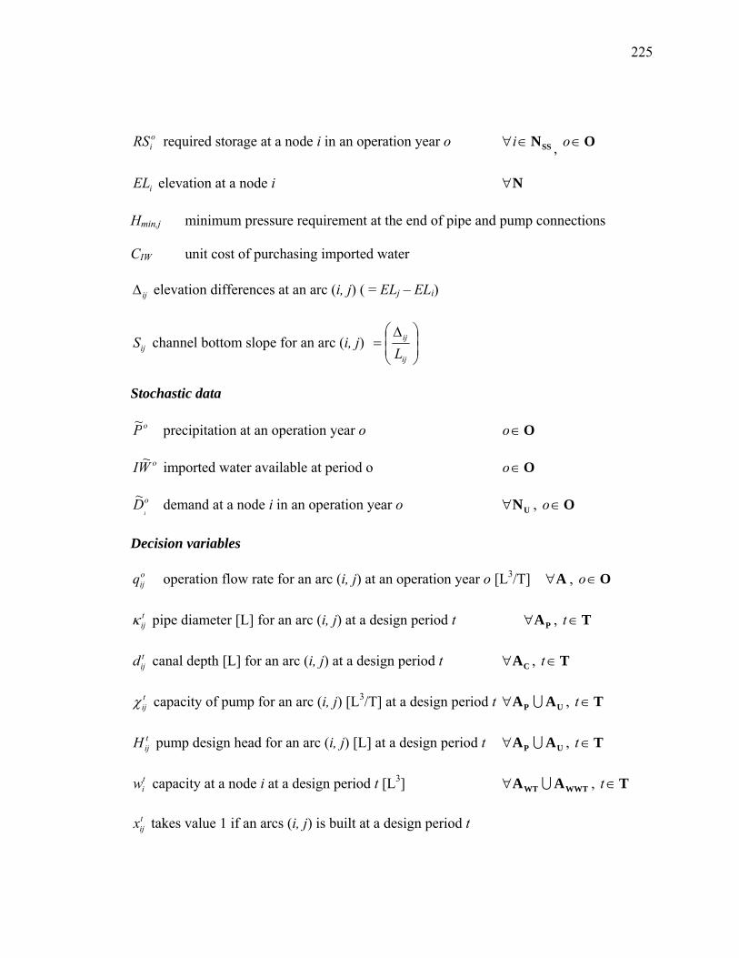
225
oiRS required storage at a node i in an operation year o SSN∈∀i , O∈o
iEL elevation at a node i N∀
Hmin,j minimum pressure requirement at the end of pipe and pump connections
CIW unit cost of purchasing imported water
ij∆ elevation differences at an arc (i, j) ( = ELj – ELi)
ijS channel bottom slope for an arc (i, j) ⎟⎟⎠
⎞⎜⎜⎝
⎛ ∆=
ij
ij
L
Stochastic data
oP~ precipitation at an operation year o O∈o
oWI ~ imported water available at period o O∈o
oi
D~ demand at a node i in an operation year o UN∀ , O∈o
Decision variables
oijq operation flow rate for an arc (i, j) at an operation year o [L3/T] A∀ , O∈o
tijκ pipe diameter [L] for an arc (i, j) at a design period t PA∀ , T∈t
tijd canal depth [L] for an arc (i, j) at a design period t CA∀ , T∈t
tijχ capacity of pump for an arc (i, j) [L3/T] at a design period t UP AA U∀ , T∈t
tijH pump design head for an arc (i, j) [L] at a design period t UP AA U∀ , T∈t
tiw capacity at a node i at a design period t [L3] WWTWT AA U∀ , T∈t
tijx takes value 1 if an arcs (i, j) is built at a design period t
226
and 0 otherwise PA∀ , T∈t
tijµ takes value 1 if a pump in an arcs (i, j) is built at a design period t
and 0 otherwise UA∀ , T∈t
7. REFERENCES
Ben-Tal ,A. and Nemirovski, A. (1999). “Robust solutions of uncertain linear programs.”
OR Letters, 25, 1-13.
Ben-Tal, A. and Nemirovski, A. (2000). “Robust solutions of Linear Programming
problems contaminated with uncertain data.” Mathematical Programming, 88, 411-
424.
Bertsimas, D. and Sim, M. (2004). “The price of robustness.” Operations Research,
52(1), 35 – 53.
Clark, R. M, Sivaganesan, M., Selvakumar, A., and Sethi, V. (2002). “Cost models for
water supply distribution systems.” Journal of Water Resources Planning and
Management, 128(5), 312-321.
El-Ghaoui, L. and Lebret, H. (1997). “Robust solutions to least-square problems to
uncertain data matrices.” SIAM Journal on Matrix Analysis and Applications, 18,
1035-1064.
El-Ghaoui, L., Oustry, F. and Lebret, H. (1998). “Robust solutions to uncertain
semidefinite programs.” SIAM Journal on Optimization, 9, 33-52.
227
Elshorbagy, W., Yakowitz, D., and Lansey, K. (1997). “Design of engineering systems
using a stochastic decomposition approach.” Engineering Optimization, 27(4), 279-
302.
Fiering, M. B. and Matalas, N. C. (1990). Decision making under uncertainty, climate
change and U.S. water resources, P. E. Waggoner, ed., John Wiley & Sons, Inc.,
New York, N.Y.
Jenkins, M. W. and Lund, J. R. (2000). “Integrating yield and shortage management
under multiple uncertainties.” Journal of Water Resources Planning and
Management, 126(5), 288-297.
Lund, G. R. and Israel, M. (1995). “Optimization of transfer in urban water supply
planning.” Journal of Water Resources Planning And Management, 121(1), 41-48.
Mulvey, J. M., Vanderbei, R. J., and Zenios, S. A. (1995). “Robust optimization of large-
scale systems.” Operations Research, 43(2), 264-281.
Sahinidis, N. and Tawarmalani, M. (2005). GAMS/BARON Solver Manual
Soyster, A. L. (1973). “Convex programming with set-inclusive constraints and
applications to inexact linear programming.” Operations Research, 21, 1154-1157.
Tang, C. C., Brill, E. D., and Pfeffer, J. T. (1987). “Optimization techniques for
secondary wastewater treatment system.” Journal of Environmental Engineering,
113(5), 935-951.
US. Amy Corps of Engineers, (1980). Methodology for areawide planning studies.
Engineer Technical. Letter No. 1110-2-502, Washington, D.C.
228
Watkins, D. W. and McKinney, D. C. (1997). “Finding robust solutions to water
resources problems.” Journal of Water Resources Planning and Management, 123(1),
49 – 58.
Wilchfort, G. and Lund, J. R. (1997). “Shortage management modeling for urban water
supply systems.” Journal of Water Resources Planning and Management, 123(4),
250-258.
Walski, T. M., Brill, E. D., Gessler, J., Goulter, I. C., Jeppson, R. M., Lansey, K., Lee,
H., Liebman, J. C., Mays, L., Morgan, D. R., and Ormsbee, L. (1987). “Battle of the
network models: epilogue.” Journal of Water Resources Planning and Management,
113(2), 191-203.
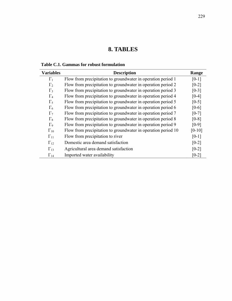
229
8. TABLES
Table C.1. Gammas for robust formulation
Variables Description Range Γ1 Flow from precipitation to groundwater in operation period 1 [0-1] Γ2 Flow from precipitation to groundwater in operation period 2 [0-2] Γ3 Flow from precipitation to groundwater in operation period 3 [0-3] Γ4 Flow from precipitation to groundwater in operation period 4 [0-4] Γ5 Flow from precipitation to groundwater in operation period 5 [0-5] Γ6 Flow from precipitation to groundwater in operation period 6 [0-6] Γ7 Flow from precipitation to groundwater in operation period 7 [0-7] Γ8 Flow from precipitation to groundwater in operation period 8 [0-8] Γ9 Flow from precipitation to groundwater in operation period 9 [0-9] Γ10 Flow from precipitation to groundwater in operation period 10 [0-10] Γ11 Flow from precipitation to river [0-1] Γ12 Domestic area demand satisfaction [0-2] Γ13 Agricultural area demand satisfaction [0-2] Γ14 Imported water availability [0-2]
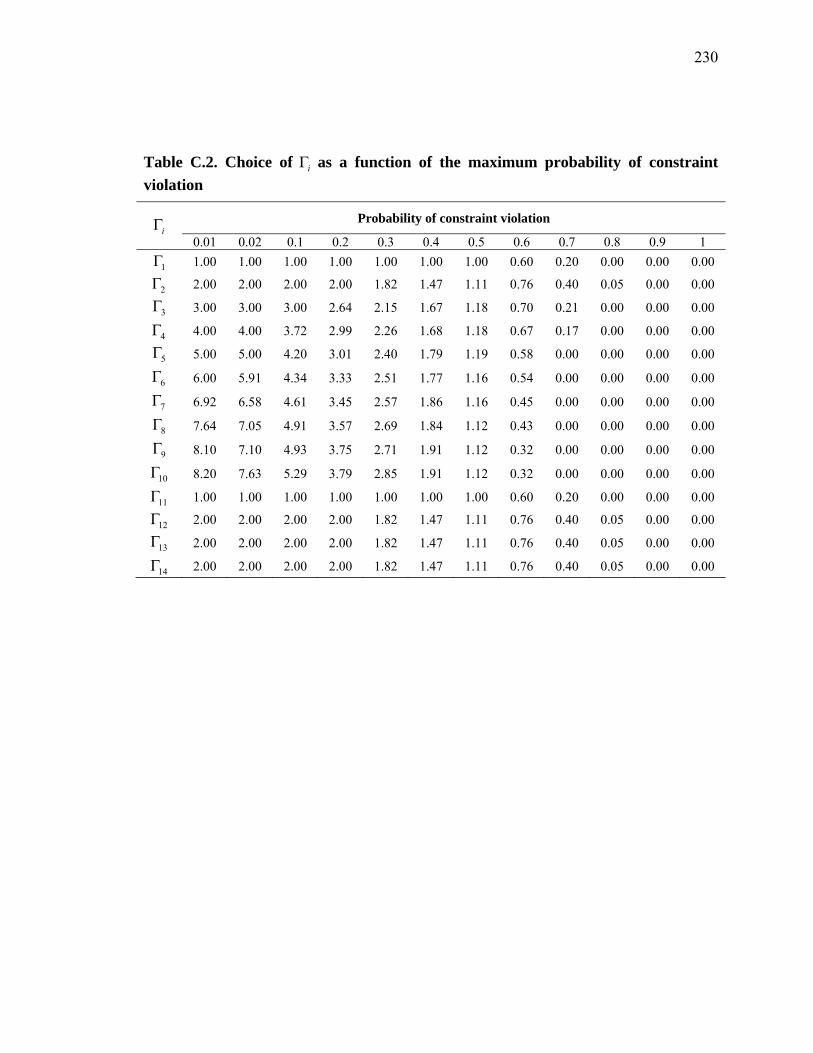
230
Table C.2. Choice of iΓ as a function of the maximum probability of constraint violation
iΓ Probability of constraint violation
0.01 0.02 0.1 0.2 0.3 0.4 0.5 0.6 0.7 0.8 0.9 1
1Γ 1.00 1.00 1.00 1.00 1.00 1.00 1.00 0.60 0.20 0.00 0.00 0.00
2Γ 2.00 2.00 2.00 2.00 1.82 1.47 1.11 0.76 0.40 0.05 0.00 0.00
3Γ 3.00 3.00 3.00 2.64 2.15 1.67 1.18 0.70 0.21 0.00 0.00 0.00
4Γ 4.00 4.00 3.72 2.99 2.26 1.68 1.18 0.67 0.17 0.00 0.00 0.00
5Γ 5.00 5.00 4.20 3.01 2.40 1.79 1.19 0.58 0.00 0.00 0.00 0.00
6Γ 6.00 5.91 4.34 3.33 2.51 1.77 1.16 0.54 0.00 0.00 0.00 0.00
7Γ 6.92 6.58 4.61 3.45 2.57 1.86 1.16 0.45 0.00 0.00 0.00 0.00
8Γ 7.64 7.05 4.91 3.57 2.69 1.84 1.12 0.43 0.00 0.00 0.00 0.00
9Γ 8.10 7.10 4.93 3.75 2.71 1.91 1.12 0.32 0.00 0.00 0.00 0.00
10Γ 8.20 7.63 5.29 3.79 2.85 1.91 1.12 0.32 0.00 0.00 0.00 0.00
11Γ 1.00 1.00 1.00 1.00 1.00 1.00 1.00 0.60 0.20 0.00 0.00 0.00
12Γ 2.00 2.00 2.00 2.00 1.82 1.47 1.11 0.76 0.40 0.05 0.00 0.00
13Γ 2.00 2.00 2.00 2.00 1.82 1.47 1.11 0.76 0.40 0.05 0.00 0.00
14Γ 2.00 2.00 2.00 2.00 1.82 1.47 1.11 0.76 0.40 0.05 0.00 0.00
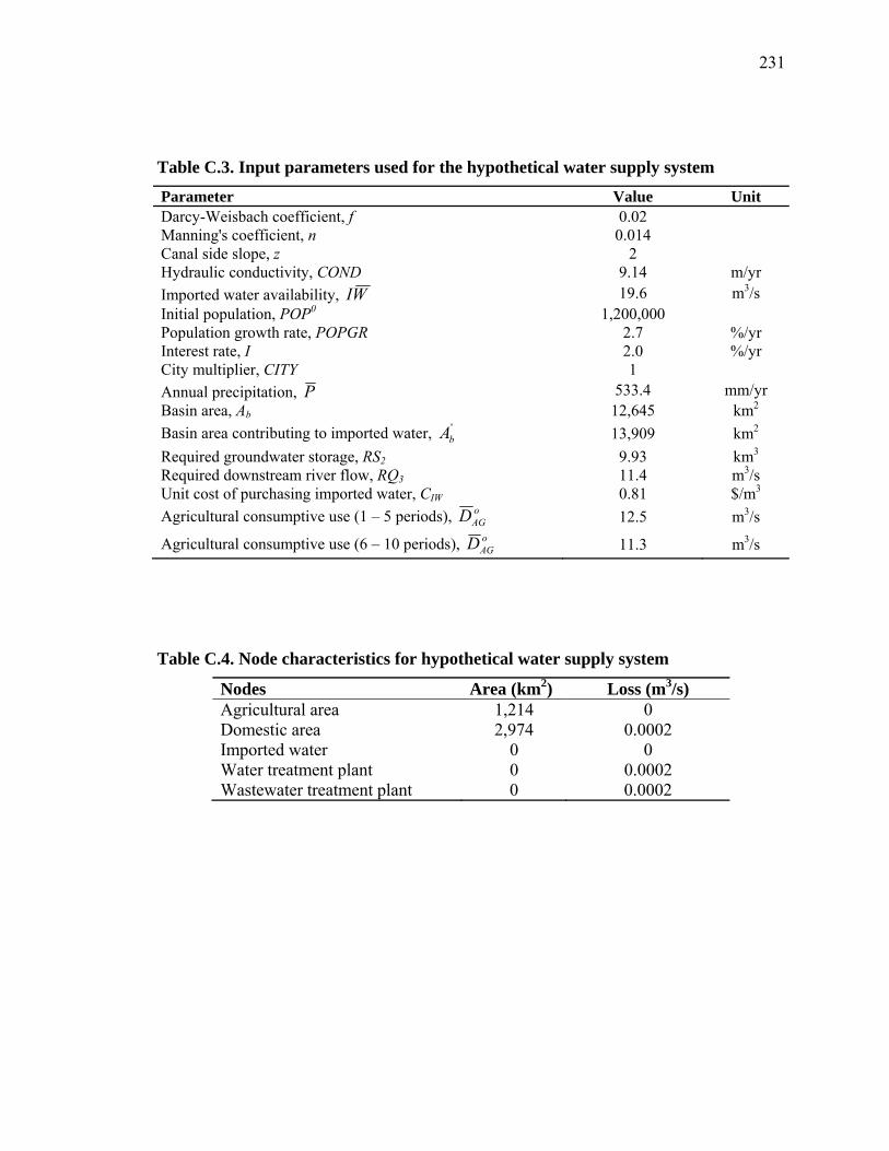
231
Table C.3. Input parameters used for the hypothetical water supply system
Parameter Value Unit Darcy-Weisbach coefficient, f 0.02 Manning's coefficient, n 0.014 Canal side slope, z 2 Hydraulic conductivity, COND 9.14 m/yr Imported water availability, WI 19.6 m3/s Initial population, POP0 1,200,000 Population growth rate, POPGR 2.7 %/yr Interest rate, I 2.0 %/yr City multiplier, CITY 1 Annual precipitation, P 533.4 mm/yr Basin area, Ab 12,645 km2 Basin area contributing to imported water, '
bA 13,909 km2 Required groundwater storage, RS2 9.93 km3 Required downstream river flow, RQ3 11.4 m3/s Unit cost of purchasing imported water, CIW 0.81 $/m3 Agricultural consumptive use (1 – 5 periods), o
AGD 12.5 m3/s
Agricultural consumptive use (6 – 10 periods), oAGD 11.3 m3/s
Table C.4. Node characteristics for hypothetical water supply system
Nodes Area (km2) Loss (m3/s) Agricultural area 1,214 0 Domestic area 2,974 0.0002 Imported water 0 0 Water treatment plant 0 0.0002 Wastewater treatment plant 0 0.0002
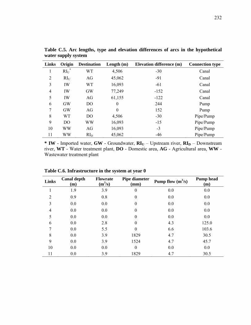
232
Table C.5. Arc lengths, type and elevation differences of arcs in the hypothetical water supply system
Links Origin Destination Length (m) Elevation difference (m) Connection type 1 RIU
* WT 4,506 -30 Canal 2 RIU AG 45,062 -91 Canal 3 IW WT 16,093 -61 Canal 4 IW GW 77,249 -152 Canal 5 IW AG 61,155 -122 Canal 6 GW DO 0 244 Pump 7 GW AG 0 152 Pump 8 WT DO 4,506 -30 Pipe/Pump 9 DO WW 16,093 -15 Pipe/Pump 10 WW AG 16,093 -3 Pipe/Pump 11 WW RID 45,062 -46 Pipe/Pump
* IW - Imported water, GW - Groundwater, RIU – Upstream river, RID – Downstream river, WT - Water treatment plant, DO - Domestic area, AG - Agricultural area, WW - Wastewater treatment plant
Table C.6. Infrastructure in the system at year 0
Links Canal depth (m)
Flowrate (m3/s)
Pipe diameter (mm) Pump flow (m3/s) Pump head
(m) 1 1.9 3.9 0 0.0 0.0 2 0.9 0.8 0 0.0 0.0 3 0.0 0.0 0 0.0 0.0 4 0.0 0.0 0 0.0 0.0 5 0.0 0.0 0 0.0 0.0 6 0.0 2.8 0 4.3 125.0 7 0.0 5.5 0 6.6 103.6 8 0.0 3.9 1829 4.7 30.5 9 0.0 3.9 1524 4.7 45.7 10 0.0 0.0 0 0.0 0.0 11 0.0 3.9 1829 4.7 30.5
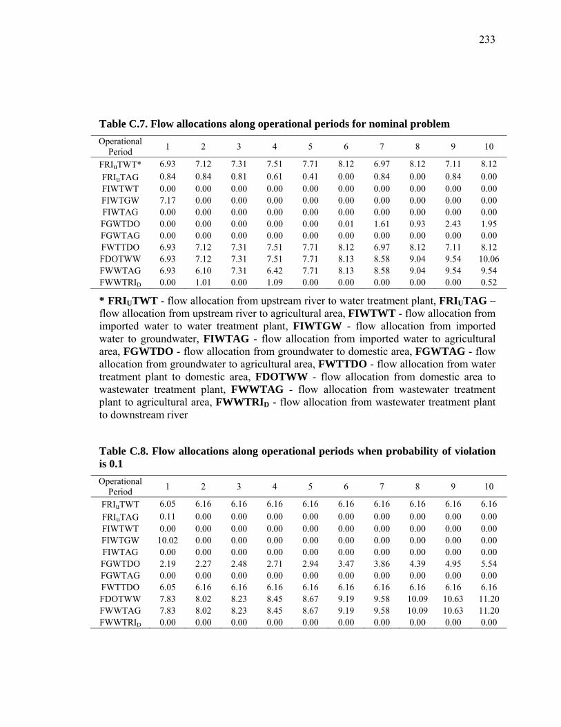
233
Table C.7. Flow allocations along operational periods for nominal problem Operational
Period 1 2 3 4 5 6 7 8 9 10
FRIuTWT* 6.93 7.12 7.31 7.51 7.71 8.12 6.97 8.12 7.11 8.12 FRIuTAG 0.84 0.84 0.81 0.61 0.41 0.00 0.84 0.00 0.84 0.00 FIWTWT 0.00 0.00 0.00 0.00 0.00 0.00 0.00 0.00 0.00 0.00 FIWTGW 7.17 0.00 0.00 0.00 0.00 0.00 0.00 0.00 0.00 0.00 FIWTAG 0.00 0.00 0.00 0.00 0.00 0.00 0.00 0.00 0.00 0.00 FGWTDO 0.00 0.00 0.00 0.00 0.00 0.01 1.61 0.93 2.43 1.95 FGWTAG 0.00 0.00 0.00 0.00 0.00 0.00 0.00 0.00 0.00 0.00 FWTTDO 6.93 7.12 7.31 7.51 7.71 8.12 6.97 8.12 7.11 8.12 FDOTWW 6.93 7.12 7.31 7.51 7.71 8.13 8.58 9.04 9.54 10.06 FWWTAG 6.93 6.10 7.31 6.42 7.71 8.13 8.58 9.04 9.54 9.54 FWWTRID 0.00 1.01 0.00 1.09 0.00 0.00 0.00 0.00 0.00 0.52
* FRIUTWT - flow allocation from upstream river to water treatment plant, FRIUTAG – flow allocation from upstream river to agricultural area, FIWTWT - flow allocation from imported water to water treatment plant, FIWTGW - flow allocation from imported water to groundwater, FIWTAG - flow allocation from imported water to agricultural area, FGWTDO - flow allocation from groundwater to domestic area, FGWTAG - flow allocation from groundwater to agricultural area, FWTTDO - flow allocation from water treatment plant to domestic area, FDOTWW - flow allocation from domestic area to wastewater treatment plant, FWWTAG - flow allocation from wastewater treatment plant to agricultural area, FWWTRID - flow allocation from wastewater treatment plant to downstream river
Table C.8. Flow allocations along operational periods when probability of violation is 0.1 Operational
Period 1 2 3 4 5 6 7 8 9 10
FRIuTWT 6.05 6.16 6.16 6.16 6.16 6.16 6.16 6.16 6.16 6.16 FRIuTAG 0.11 0.00 0.00 0.00 0.00 0.00 0.00 0.00 0.00 0.00 FIWTWT 0.00 0.00 0.00 0.00 0.00 0.00 0.00 0.00 0.00 0.00 FIWTGW 10.02 0.00 0.00 0.00 0.00 0.00 0.00 0.00 0.00 0.00 FIWTAG 0.00 0.00 0.00 0.00 0.00 0.00 0.00 0.00 0.00 0.00 FGWTDO 2.19 2.27 2.48 2.71 2.94 3.47 3.86 4.39 4.95 5.54 FGWTAG 0.00 0.00 0.00 0.00 0.00 0.00 0.00 0.00 0.00 0.00 FWTTDO 6.05 6.16 6.16 6.16 6.16 6.16 6.16 6.16 6.16 6.16 FDOTWW 7.83 8.02 8.23 8.45 8.67 9.19 9.58 10.09 10.63 11.20 FWWTAG 7.83 8.02 8.23 8.45 8.67 9.19 9.58 10.09 10.63 11.20 FWWTRID 0.00 0.00 0.00 0.00 0.00 0.00 0.00 0.00 0.00 0.00
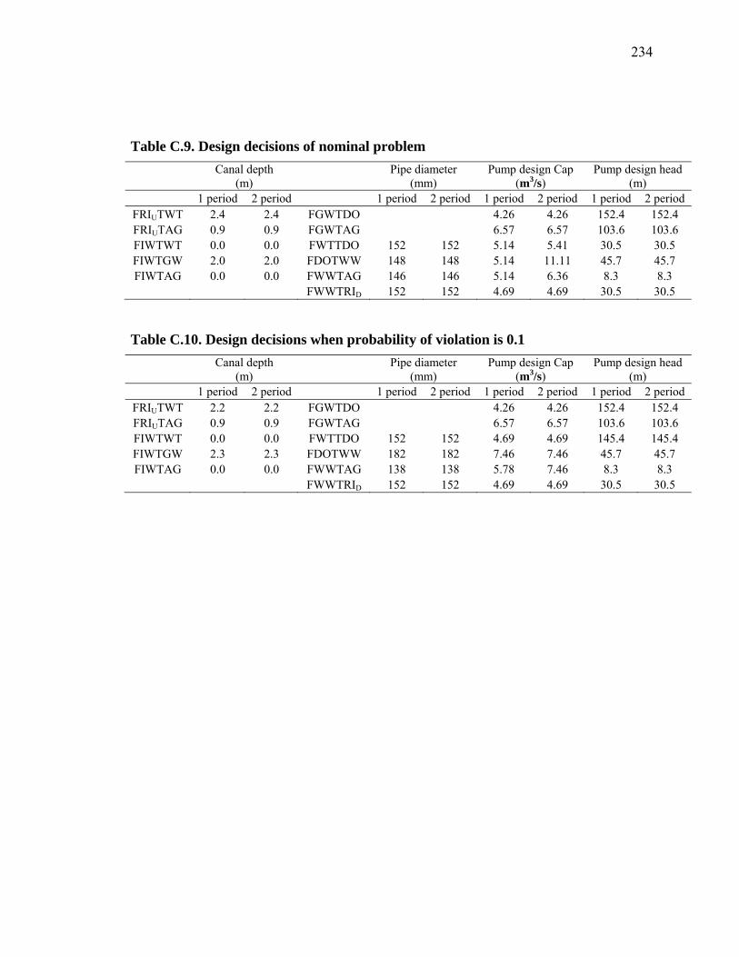
234
Table C.9. Design decisions of nominal problem
Canal depth (m)
Pipe diameter (mm)
Pump design Cap (m3/s)
Pump design head (m)
1 period 2 period 1 period 2 period 1 period 2 period 1 period 2 period FRIUTWT 2.4 2.4 FGWTDO 4.26 4.26 152.4 152.4 FRIUTAG 0.9 0.9 FGWTAG 6.57 6.57 103.6 103.6 FIWTWT 0.0 0.0 FWTTDO 152 152 5.14 5.41 30.5 30.5 FIWTGW 2.0 2.0 FDOTWW 148 148 5.14 11.11 45.7 45.7 FIWTAG 0.0 0.0 FWWTAG 146 146 5.14 6.36 8.3 8.3
FWWTRID 152 152 4.69 4.69 30.5 30.5
Table C.10. Design decisions when probability of violation is 0.1
Canal depth (m)
Pipe diameter (mm)
Pump design Cap (m3/s)
Pump design head (m)
1 period 2 period 1 period 2 period 1 period 2 period 1 period 2 period FRIUTWT 2.2 2.2 FGWTDO 4.26 4.26 152.4 152.4 FRIUTAG 0.9 0.9 FGWTAG 6.57 6.57 103.6 103.6 FIWTWT 0.0 0.0 FWTTDO 152 152 4.69 4.69 145.4 145.4 FIWTGW 2.3 2.3 FDOTWW 182 182 7.46 7.46 45.7 45.7 FIWTAG 0.0 0.0 FWWTAG 138 138 5.78 7.46 8.3 8.3
FWWTRID 152 152 4.69 4.69 30.5 30.5
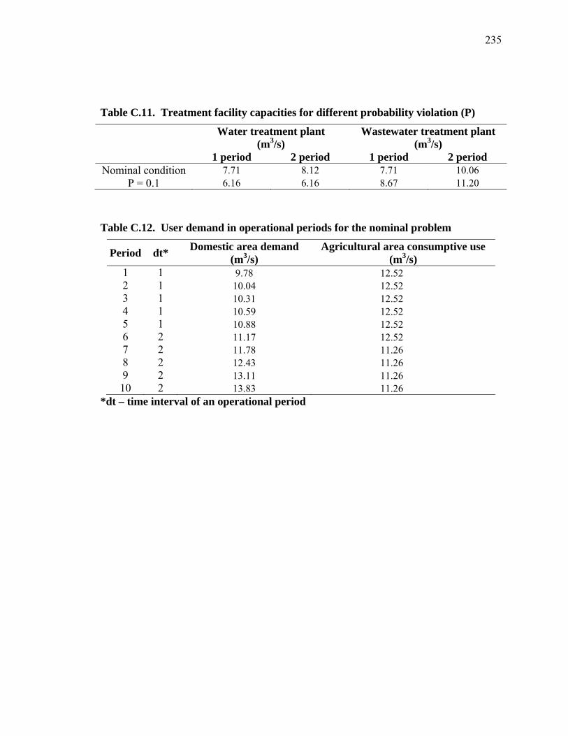
235
Table C.11. Treatment facility capacities for different probability violation (P)
Water treatment plant
(m3/s) Wastewater treatment plant
(m3/s) 1 period 2 period 1 period 2 period
Nominal condition 7.71 8.12 7.71 10.06 P = 0.1 6.16 6.16 8.67 11.20
Table C.12. User demand in operational periods for the nominal problem
Period dt* Domestic area demand (m3/s)
Agricultural area consumptive use (m3/s)
1 1 9.78 12.52 2 1 10.04 12.52 3 1 10.31 12.52 4 1 10.59 12.52 5 1 10.88 12.52 6 2 11.17 12.52 7 2 11.78 11.26 8 2 12.43 11.26 9 2 13.11 11.26 10 2 13.83 11.26
*dt – time interval of an operational period
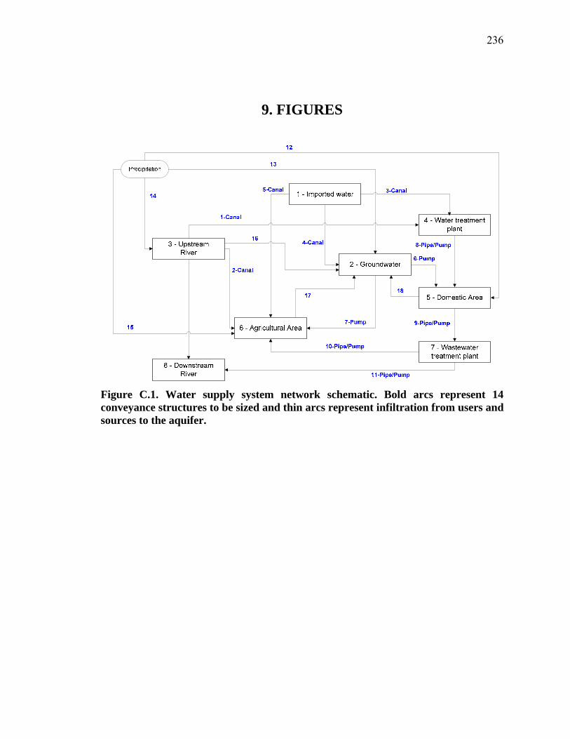
236
9. FIGURES
Figure C.1. Water supply system network schematic. Bold arcs represent 14 conveyance structures to be sized and thin arcs represent infiltration from users and sources to the aquifer.
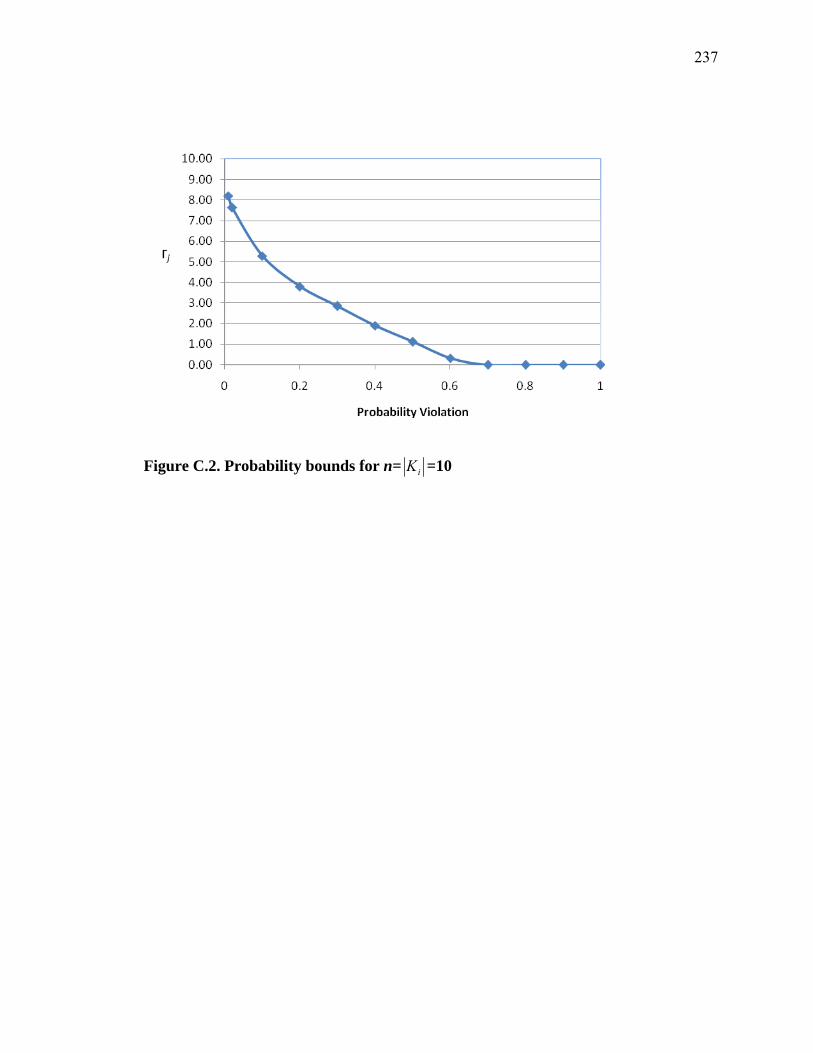
237
Figure C.2. Probability bounds for n= iK =10
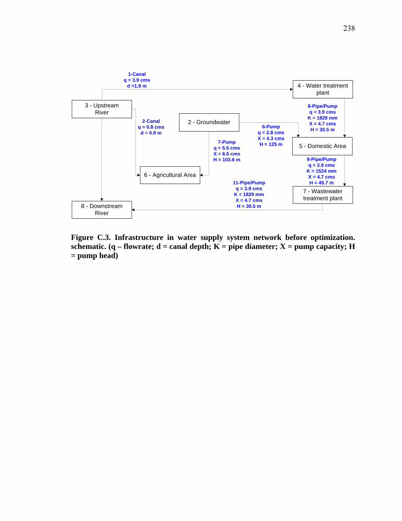
238
8 - DownstreamRiver
2 - Groundwater
5 - Domestic Area
6 - Agricultural Area
7 - Wastewater treatment plant
4 - Water treatment plant
2-Canalq = 0.8 cmsd = 0.9 m
8-Pipe/Pumpq = 3.9 cms
K = 1829 mmX = 4.7 cmsH = 30.5 m6-Pump
q = 2.8 cmsX = 4.3 cmsH = 125 m
11-Pipe/Pumpq = 3.9 cms
K = 1829 mmX = 4.7 cmsH = 30.5 m
1-Canalq = 3.9 cms
d =1.9 m
3 - UpstreamRiver
7-Pumpq = 5.5 cmsX = 6.6 cmsH = 103.6 m 9-Pipe/Pump
q = 3.9 cmsK = 1524 mmX = 4.7 cmsH = 45.7 m
Figure C.3. Infrastructure in water supply system network before optimization. schematic. (q – flowrate; d = canal depth; K = pipe diameter; X = pump capacity; H = pump head)
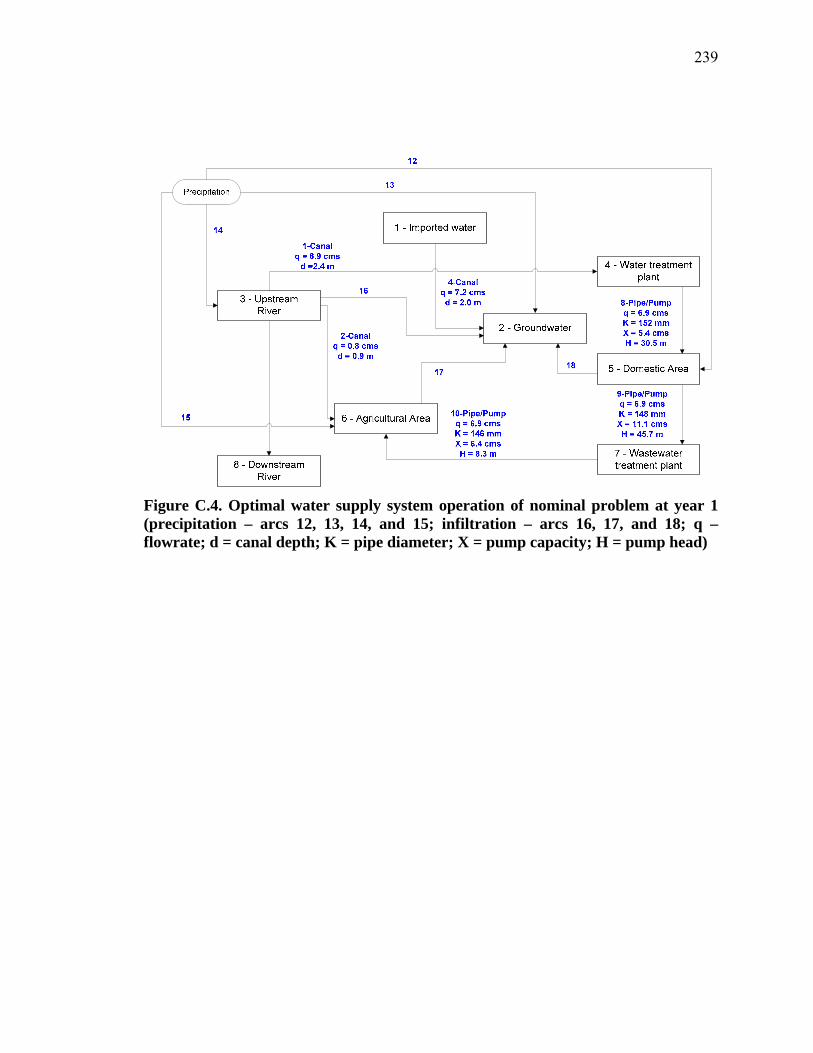
239
Figure C.4. Optimal water supply system operation of nominal problem at year 1 (precipitation – arcs 12, 13, 14, and 15; infiltration – arcs 16, 17, and 18; q – flowrate; d = canal depth; K = pipe diameter; X = pump capacity; H = pump head)
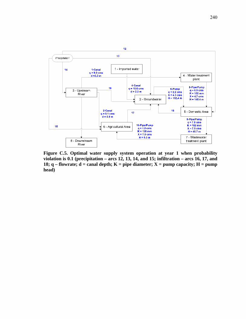
240
Figure C.5. Optimal water supply system operation at year 1 when probability violation is 0.1 (precipitation – arcs 12, 13, 14, and 15; infiltration – arcs 16, 17, and 18; q – flowrate; d = canal depth; K = pipe diameter; X = pump capacity; H = pump head)
241
Figure C.6. Optimal total cost of the water supply system as a function of the probability bound of constraint violation
242
Figure C.7. Total amount of imported water purchased as a function of the probability bound of constraint violation