water resources research report - idf-cc-uwo.ca · • idf update algorithm: the equidistant...
TRANSCRIPT

THE UNIVERSITY OF WESTERN ONTARIO
DEPARTMENT OF CIVIL AND
ENVIRONMENTAL ENGINEERING
Water Resources Research Report
Report No: 089
Date: February 2015
Computerized Tool for the Development of
Intensity-Duration-Frequency Curves under a
Changing Climate
Technical Manual v.1.1
By:
Roshan K. Srivastav
Andre Schardong
and
Slobodan P. Simonovic
ISSN: (print) 1913-3200; (online) 1913-3219;
ISBN: (print) 978-0-7714-3087-9; (online) 978-0-7714-3088-6;
I
Computerized tool for the Development of Intensity-Duration-
Frequency Curves under a Changing Climate
www.idf-cc-uwo.ca
Technical Manual
Version 1.1
February, 2015
By
Roshan K. Srivastav
Andre Schardong
and
Slobodan P. Simonovic
Department of Civil and Environmental Engineering
The University of Western Ontario
London, Ontario, Canada

II
Executive Summary
Climate change and its effects on nature, humans and the world economy are major research
challenges of recent times. Climate observations and numerous studies clearly indicate that
climate is changing rapidly under the influence of changing chemical composition of the
atmosphere, major modifications of land use and ever-growing population. The increase of
concentration of greenhouse gases (GHG) seems to be one of the major driving forces behind
climate change.
Global warming has already affected the hydrological and ecological cycle of the earth’s system.
Among the noticeable modifications of the hydrologic cycle is the change in frequency and
intensity of extreme rainfall events, which in many cases result in severe floods. Most of
Canada’s existing water resources infrastructure has been designed based on the assumption that
historical climate is a good predictor of the future. It is now realized that the historic climate will
not be representative of future conditions and new and existing water resource systems must be
designed or retrofitted to take into consideration changing climate conditions.
Rainfall intensity-duration-frequency (IDF) curves are one of the most important tools for
design, operation and maintenance of a variety of water management infrastructures, including
sewers, storm water management ponds, street curbs and gutters, catch basins, swales, among a
significant variety of other types of infrastructure. Currently, IDF curves are usually developed
using historical observed data with the assumption that the same underlying processes will
govern future rainfall patterns and resulting IDF curves. This assumption is not valid under
changing climatic conditions. Global climate models (GCM) provide understanding of climate
change under different future emission scenarios, also known as representative concentration
pathways (RCP), and provide a way to update IDF curves under a changing climate. More than
40 GCMs have been developed by various research organizations around the world. However,
these GCMs are built to project climate change on large spatial and temporal scales and therefore
use of GCMs for modification of IDF curves, which are local or regional in nature, requires some
additional steps.

III
The work presented in this manual is part of the project “Computerized IDF_CC Tool for the
Development of Intensity-Duration-Frequency Curves under a Changing Climate” supported by
Canadian Water Network. The project focuses on (i) the development of a new methodology for
updating IDF curves; and (ii) building a web based IDF update tool. This technical manual
provides a detailed description of the mathematical models and procedures used within the
IDF_CC tool. The accompanied document presents the User’s Manual for the IDF_CC tool
entitled “Computerized IDF_CC Tool for the Development of Intensity-Duration-Frequency-
Curves under a Changing Climate - User’s Manual” referred further as UserMan.
The remainder of the manual is organized as follows. Section 1 introduces the issue of IDF
curves under changing climate. In section 2, a brief background review of IDF curves and
processes for updating IDF curve information is provided. Section 3 presents the mathematical
models that are used for: (i) Fitting probability distributions; (ii) Estimating parameters; (iii)
Spatially interpolating GCM data to observed stations; (iv) Selecting GCM models; and (v)
Updating IDF curves. Finally, a summary and the conclusions are outlined in section 4.

IV
Contents
Executive Summary ....................................................................................................................................... II
List of Figures ................................................................................................................................................ V
List of Tables ................................................................................................................................................. V
1.0 Introduction ............................................................................................................................................ 1
2.0 Background ............................................................................................................................................. 5
2.1 Intensity-Duration-Frequency Curves ................................................................................................. 5
2.2 Updating IDF Curves .......................................................................................................................... 6
2.3 Global Climate Models (GCM) and Emission Scenarios ................................................................... 8
2.4 Selection of GCM models ................................................................................................................. 11
2.5 Historical Data .................................................................................................................................. 11
3.0 Mathematical Models and Procedures used by IDF_CC ....................................................................... 12
3.1 Statistical Analysis ............................................................................................................................ 12
3.1.1 Probability Distribution Function .............................................................................................. 12
3.1.2 Parameter Estimation ................................................................................................................. 13
3.1.4 Spatial Interpolation of GCM data ............................................................................................. 15
3.2 Selection of GCM Using Quantile Regression ................................................................................. 16
3.2.1 Quantile Regression Based Skill Score Method (QRSS) ........................................................... 17
3.3 Updating IDF curves under a Changing Climate .............................................................................. 20
3.3.1 Equidistance Quantile Matching Method ................................................................................... 21
4. Summary and Conclusion........................................................................................................................ 28
References ................................................................................................................................................... 28
Acknowledgements ..................................................................................................................................... 32
Appendix – A: MATLAB code to update IDF curves ................................................................................... 33
Appendix – B: GCMs used in IDF_CC tool .................................................................................................. 37
Appendix – C: Case Example: Station London ............................................................................................ 39
Appendix – E: Journal paper on Quantile Regression for selection of GCMs (Under Review) ................... 45
Appendix – F: Journal paper on equidistance quantile matching method for updating IDF curves under
climate change ............................................................................................................................................ 46
Appendix – G: List of Previous Reports in the Series ................................................................................ 47

V
List of Figures
Figure 1: Changes in observed precipitation from 1901 to 2010 and from 1951 to 2010 (after
IPCC 2013)
Figure 2: Changes in annual mean precipitation for 2081-2100 relative to 1986-2005 under the
Representative Concentration Pathway RCP 8.5.(after IPCC 2013) (see Appendix B)
Figure 3: Concept of Equidistance quantile matching method for updating IDF curves
Figure 4: Equidistance Quantile-Matching Method for generating future IDF curves under
Climate Change
List of Tables
Table 1: Summary of AR5 Assessments for Extreme Precipitation
Table 2: Comparison of Dynamic downscaling and Statistical downscaling
Table 3: Comparison of method of moments and L-moments

1
1.0 Introduction
Changes in climate conditions observed over the last few decades are considered to be the cause
of change in magnitude and frequency of occurrence of extreme events (IPCC 2013). The Fifth
Assessment Report (AR5) of the Intergovernmental Panel on Climate Change (IPCC 2013) has
indicated a global surface temperature increase of 0.3 to 4.8 °C by the year 2100 compared to the
reference period 1986-2005 with more significant changes in tropics and subtropics than in mid-
latitudes. It is expected that rising temperature will have a major impact on the magnitude and
frequency of extreme precipitation events in some regions (Barnett et al. 2006; Wilcox et al.
2007; Allan et al. 2008; Solaiman et al. 2011). Incorporating these expected changes in planning,
design, operations and maintenance of water infrastructure would reduce unseen future
uncertainties that may result from increasing frequency and magnitude of extreme rainfall
events.
According to the AR5, heavy precipitation events are expected to increase in frequency,
intensity, and/or amount of precipitation under changing climate conditions. Table 1 summarizes
assessments made regarding heavy precipitation in AR5 (IPCC 2013 – Table SPM.1).
Table 1: Summary of AR5 Assessments for Extreme Precipitation
Assessment that
changes occurred since
1950
Assessment of a
human contribution to
observed changes
Likelihood of further changes
Early 21st century Late 21st century
Likely more land areas
with increases than
decreases
Medium Confidence
Likely over many land
areas
Very likely over most of
the mid-latitude land
masses and over wet
tropical areas
Likely more land areas
with increases than
decreases
Medium confidence Likely over many areas
Likely over most land
areas More likely than not
Very likely over most
land areas

2
Since it is evident that the global temperature is increasing with climate change, it follows that
the saturation vapor pressure of the air will increase, as this is a function of air temperature.
Further, it is observed that the historical precipitation data has shown considerable changes in
trends over the last 50 years (Fig. 1 and 2). These changes are likely to intensify with increases
in global temperature (IPCC 2013).
Evaluation of change in precipitation intensity and frequency is critical as these data are used
directly in design and operation of water infrastructure. However, assessment of climate change
impacts and the implementation of climate change research is a challenge for many practitioners.
Figure 1: Changes in observed precipitation from 1901 to 2010 and from 1951 to 2010 (after IPCC
2013)
Figure 2: Changes in annual mean precipitation for 2081-2100 relative to 1986-2005 under
the Representative Concentration Pathway RCP 8.5. (after IPCC 2013) (see Appendix B)

3
Practitioner application of climate change science remains a challenge for several reasons,
including: 1) the complexity of and difficulty in implementing climate change impact assessment
methods, which are based on heavy analytical procedures; 2) the academic and scientific
communities’ focus on publishing research findings under the rigorous peer review processes
with limited attention given to practical implementation of findings; 3) political dimensions of
climate change issues; and 4) a high level of uncertainty with respect to future climate
projections in the presence of multiple climate models and emission scenarios.
This project aimed to develop and implement a generic and simple tool to allow practitioners to
easily incorporate impacts of climate change, in form of updated IDF curves, into water
infrastructure design and management. To accomplish this task, a web interface based tool has
been developed (referred to as the IDF_CC tool), consisting of friendly user interface with a
powerful database system and sophisticated, but efficient, methodology for the update of IDF
curves.
Intensity duration frequency (IDF) curves are typically developed by fitting a theoretical
probability distribution to an annual maximum precipitation (AMP) time series. AMP data is
fitted using extreme value distributions like Gumbel, Generalized Extreme Value (GEV), Log
Pearson, Log Normal, among other approaches. The IDF curves provide precipitation
accumulation depths for various return periods (T) and different durations, usually, 5, 10, 15, 20
30 minutes, 1, 2, 6, 12, 18 and 24 hours. Durations exceeding 24 hours may also be used,
depending on the application of IDF curves. Hydrologic design of storm sewers, culverts,
detention basins and other elements of storm water management systems is typically performed
based on specified design storms derived from the IDF curves (Solaiman and Simonovic, 2010;
Peck et al., 2012).
The web based IDF_CC tool is a decision support system (DSS). As such, it includes traditional
DSS components including a user interface, database and model base. 1 One of the major
components of the IDF_CC decision support system is a model base that includes a set of
mathematical models and procedures for updating IDF curves. These mathematical models are
1 For a detailed description of DSS components, see UserMan Section 1.

4
an important part of the IDF_CC tool and are responsible for the calculations required to develop
the IDF curves based on historical data and for updating IDFs to reflect future climatic
conditions. The models and procedures used within the IDF_CC tool include:
• Statistical analysis algorithms: statistical analysis is applied to fit the selected theoretical
probability distributions to both historical and future precipitation data. To fit the data
Gumbel distribution is used in this tool They are fitted using method of moments. The
GCM data used in statistical analysis are spatially interpolated from the nearest grid
points using the inverse distance method.
• Optimization algorithm: an algorithm used to fit the analytical relationship to an IDF
curve.
• GCM Selection algorithm: a quantile regression based algorithm applied to select and/or
rank the GCM models according to their skill.2
• IDF update algorithm: the equidistant quantile matching – EQM algorithm is applied to
the IDF updating procedure.
This technical manual presents the details of the statistical analysis procedures, GCM selection
algorithm and IDF update algorithm. For the optimization algorithm, readers are referred to
UserMan Appendix 1.
2 The “skill” of a GCM reflects its ability to accurately simulate past or present day climates for a given region.

5
2.0 Background
2.1 Intensity-Duration-Frequency Curves
Reliable rainfall intensity estimates are necessary for hydrologic analyses, planning, management
and design of water infrastructure. Information from IDF curves is used to describe the
frequency of extreme rainfall events of various intensities and durations. The rainfall intensity-
duration-frequency (IDF) curve is one of the most common tools used in urban drainage
engineering, and application of IDF curves for a variety of water management applications has
been increasing (CSA, 2010). The guideline for ‘Development, Interpretation and Use of
Rainfall Intensity-Duration-Frequency (IDF) Information: A Guideline for Canadian Water
Resources Practitioners” developed by Canadian Standards Association (CSA, 2012) lists the
following reasons for increasing application of rainfall IDF information:
As the spatial heterogeneity of extreme rainfall patterns becomes better understood and
documented, a stronger case is made for the value of “locally relevant” IDF information.
As urban areas expand, making watersheds generally less permeable to rainfall and
runoff, many older water systems fall increasingly into deficit, failing to deliver the
services for which they were designed. Understanding the full magnitude of this deficit
requires information on the maximum inputs (extreme rainfall events) with which
drainage works must contend.
Climate change will likely result in an increase in the intensity and frequency of extreme
precipitation events in most regions in the future. As a result, IDF values will optimally
need to be updated more frequently than in the past and climate change scenarios might
eventually be drawn upon in order to inform IDF calculations.
The typical development of rainfall IDF curves involves three steps. First, a probability
distribution function (PDF) or Cumulative Distribution Function (CDF) is fitted to rainfall data
for a number of rainfall durations. Second, the maximum rainfall intensity for each time interval
is related with the corresponding return period from the cumulative distribution function. Third,
from the known cumulative frequency and given duration, the maximum rainfall intensity can be
determined using an appropriate fitted theoretical distribution functions (such as GEV, Gumbel,
Pearson Type III, etc.) (Solaiman and Simonovic 2010). The IDF_CC tool adopts Gumbel

6
distribution for fitting the annual maximum precipitation (AMP). The parameter estimation for
the selected distributions is carried out using the method of moments.
2.2 Updating IDF Curves
The main assumption in the process of developing IDF curves is that the historical series are
stationary and therefore can be used to represent the future extreme conditions. This assumption
is questionable under rapidly changing conditions, and therefore IDF curves that rely only on
historical observations will misrepresent future conditions (Sugahara et al. 2009; Milly et al.
2008). Global Climate Modeling (GCM) is one of the best ways to explicitly address changing
climate conditions for the future periods (i.e., non-stationary conditions). GCM models simulate
atmospheric patterns on larger spatial grid scales (usually greater than 100 kilometers) and hence
are unable to represent the regional scale dynamics accurately. In contrast, regional climate
models (RCM) are developed to incorporate the local-scale effects and use smaller grid scales
(usually 25 to 50 kilometers). The major shortcoming of RCMs is the computational
requirements to generate realizations for various atmospheric forcings.
Both GCM and RCM models have larger spatial scales than the size of most watersheds, which
is the relevant scale for IDF curves. Downscaling is one of the techniques to link GCM/RCM
grid scales and local study areas for the development of IDF curves under changing climate
conditions. Downscaling approaches can be broadly classified as either dynamic downscaling or
statistical downscaling. The dynamic downscaling procedure is based on limited area models or
uses higher resolution GCM/RCM models to simulate local conditions, whereas statistical
downscaling procedures are based on transfer functions which relate the GCM models with the
local study areas; that is,, a mathematical relationship is developed between the GCM output and
historically observed data for the time period of observations. Statistical downscaling procedures
are used more widely than dynamic models because of their lower computational requirements
and availability of GCM outputs for a wider range of emission scenarios. Table 2 provides
comparison between dynamic downscaling and statistical downscaling.

7
Table 2: Comparison of dynamic downscaling and statistical downscaling
Criteria Dynamic downscaling Statistical downscaling
Computational time Slower Fast
Experiments Limited realizations Multiple realizations
Complexity More complete physics Succinct physics
Examples Regional climate models,
Nested GCMs
Linear regression, Neural
network, Kernel regression
The IDF_CC tool adopts an equidistant quantile-matching (EQM) method for updating IDF
curves, developed by Srivastav et al. (2014), which can capture the distribution of changes
between the projected time period and the baseline period (temporal downscaling) in addition to
spatial downscaling the annual maximum precipitation (AMP) derived from the GCM data and
the observed sub-daily data. In the case of the EQM method, the quantile-mapping functions are
directly applied to annual maximum precipitation (AMP) to establish the statistical relationships
between the AMPs of GCM and sub-daily observed (historical) data rather than using complete
daily precipitation records. This methodology is relatively simple (in terms of modelling
complexities) and computationally efficient. Figure 3 explains a simplified approach to update
for EQM method used in IDF_CC tool to update IDF curves. The three main steps which are
involved in using EQM method are: (i) establish statistical relationship between the AMPs of the
GCM and the observed station of interest, which is referred as spatial downscaling (See Figure 3
dark brown arrow); and (ii) establish statistical relationship between the AMPs of the base period
GCM and the future period GCM, which is which is referred as temporal downscaling (See
Figure 3 black arrow); and (iii) establish statistical relationship between steps (i) and (ii) to
update the IDF curves for future periods (See Figure 3 red arrow).

8
2.3 Global Climate Models (GCM) and Representative Concentration Pathways
General Climate Models (GCM) represent the dynamics within the Earth’s atmosphere to
understand current and future climatic conditions. These models are the best tools for assessment
of the impacts of climate change. There are numerous GCMs developed by different climate
research centres. They are all based on (i) land-ocean-atmosphere coupling; (ii) greenhouse gas
emissions, and; (iii) different initial conditions representing the state of the climate system.
These models simulate global climate variables on coarse spatial grid scales (e.g., 250 km by 250
km) and are expected to mimic the dynamics of regional-scale climate conditions. The GCMs are
extended to predict the atmospheric variables under the influence of climate change due to global
warming. The amount of greenhouse gas emissions is the key variable for generating future
scenarios. Other factors that may influence the future climate include land-use, energy
production, global and regional economy and population growth.
To update the IDF curves under changing climatic conditions, the IDF_CC tool uses 22 GCMs
from different climate research centers (see UserMan: Section 3.2). The GCM outputs are
usually available in the netCDF format that is widely used for storing climate data. The IDF_CC
tool converts the netCDF files into a more efficient format in order to reduce storage space and
computational time. These converted climate data files are stored in the IDF_CC tool’s database
(see UserMan: Section 1.2). The salient features of each of the GCMs used in the IDF_CC tool is
presented in Appendix B. The data for the various GCMs can be downloaded from
GCM/RCM Daily Maximum GCM/RCM Future Daily Maximum
(RCP Scenarios)
Observed Sub-Daily Maximum Future Sub-Daily Maximum
Historical IDF Curves Updated IDF Curves
Temporal
Spat
ial
Spatial
Point Observation
Gridded Data
Figure 3: Concept of Equidistance quantile matching method for updating IDF curves

9
https://www.earthsystemgrid.org/home.htm which is a gateway for scientific data collections.
These models are adopted based on the availability of complete sets of future greenhouse gas
concentration scenarios, also known as Representative Concentration Pathways (RCPs)
described in detail in the IPCC AR5 report (See: IPCC Fifth Assessment Report – Annex 1
Table: AI.1), and briefly described below.
Based on the initial conditions that represent the state of the climate system, GCMs generate
different time series that are known as ‘Runs’. Multiple Runs are conducted to help account for
uncertainty related to initial conditions. Updating IDF curves using all the time series that
include Runs from each of the GCMs would be computationally demanding. Therefore the
IDF_CC tool provides three options (UserMan: Section 3.2), including: (i) select a GCM based
on skill score or (ii) select any model from the list of GCMs provided in the tool or (iii) select
ensemble. The selection of GCM based on skill scores will rank the models in the order of their
skill. That is, the first model listed for the user will have the highest skill score, followed
subsequently by each model ranked in order of their declining skill scores. This method
automatically allows the user to select the best GCM for updating the IDF curves. The user can
choose the second option to test any of the GCM models to update the IDF curves. The users are
encouraged to test different models due to the uncertainty associated with climate modeling
(UserMan: Section 3.2).
The Fifth Assessment Report (AR5) of the Intergovernmental Panel on Climate Change (IPCC)
introduced new future climate scenarios associated with Representative Concentration Pathways
(RCPs), which are based on time-dependent projections of atmospheric greenhouse gas (GHG)
concentrations. RCPs are scenarios that include time series of emissions and concentrations of
the full suite of greenhouse gases, aerosols and chemically active gases, as well as land use and
land cover factors (Moss et al., 2008). The word “representative” signifies that each RCP
provides only one of many possible scenarios that would lead to the specific radiative forcing3
3 Radiative forcing is the change in the net, downward minus upward, radiative flux (expressed in Wm-2) at the tropopause or top of atmosphere due to a change in external driver of climate change, such as, for example, a change in the concentration of carbon dioxide or the output of the sun (IPCC AR5, annex III)

10
characteristics. The term “pathway” emphasizes that not only the long-term concentration levels
are of interest, but also the trajectory taken over time to reach that outcome (Moss et al. 2010).
There are four RCP scenarios: RCP 2.6, RCP 4.5, RCP 6.5 and RCP 8.5. The following
definitions are adopted directly from IPCC AR5 (IPCC 2013):
RCP2.6: One pathway where radiative forcing peaks at approximately 3 W m–2 before 2100 and
then declines (the corresponding Extended Concentration Pathways4 (ECP) assuming constant
emissions after 2100).
RCP4.5 and RCP6.0: Two intermediate stabilization pathways in which radiative forcing is
stabilized at approximately 4.5 W m–2 and 6.0 W m–2 after 2100 (the corresponding ECPs
assuming constant concentrations after 2150).
RCP8.5: One high pathway for which radiative forcing reaches greater than 8.5 W m–2 by 2100
and continues to rise for some time (the corresponding ECP assuming constant emissions after
2100 and constant concentrations after 2250).
The future emission scenarios used in the IDF_CC tool are based on RCP2.6, RCP4.5 and
RCP8.5 (UserMan: Section 3.2 and 3.3). RCP2.6 represents the lower bound, followed by
RCP4.5 as an intermediate level and RCP 8.5 as the higher bound. IDF curves developed using
RCP2.6 and RCP8.5 represent the range of uncertainty or possible range of IDF curves under
changing climatic conditions. Similar to GCMs, the future emission scenarios for each GCM
(i.e., the RCPs) have different Runs based on the initial conditions imposed on the model. The
number of updated IDF curves from a particular RCP scenario will be equal to the number of
runs available for a selected GCM. The IDF_CC tool has two representations of future IDF
curves (UserMan: Section 3.3): (i) updated IDF curve for each RCP scenario where the IDF
curves are averaged from all the GCMs and their scenarios and (ii) comparison of future and
historical IDF curves.
4 Extended concentration pathways describes extensions of the RCP’s from 2100 to 2500 (IPCC AR5, annex III)

11
2.4 Selection of GCM models
According to the fifth assessment report of IPCC, there are 42 GCM models developed by
various research centres (Refer: Table AI.1 from Annex I IPCC AR5). In IDF_CC tool, adopts
only 22 GCM models out of the 42 listed GCMs because: i) Not all the GCMs generate the three
selected RCPs for future climate scenarios (i.e., RCP 2.6, 4.5 and 8.5); and ii) there are some
technical issues related to downloading (such as connection to remote servers or repositories) for
some GCM models. Currently, the IDF_CC tool uses all 22 GCMs that have all the three future
climate scenarios available for updating the IDF curves (UserMan: Section 3.2). However, the
use of all the 22 GCMs in the IDF_CC tool could be computationally demanding. In order to
reduce uncertainty due to choice of the GCMs, the tool applies a skill score algorithm to rank the
GCMs provided in the tool. The IDF_CC tool adopts a skill score based on quantile regression
(QRSS) proposed by Srivastav et al. (2015) (Appendix E) to assess the performance of different
GCM models available for use within the tool. The QRSS approach has two main components:
(i) the quantiles representing the distribution of the data; (ii) the quantile regression lines
representing the trends and heteroscedasticity across the quantiles. The QRSS has the ability to
capture (i) the distributional characteristics; and (ii) the error statistics. In order to avoid the risks
of claiming a false precision in our ability to distinguish credible from non-credible scenarios,
which could lead to bad decisions by end users IPCC typically includes most or all members of
CMIP multi-model ensembles in their uncertainty analysis. The IDF_CC tool provides an option
to the user to generate the ensemble of all the 22 GCMs.
2.5 Historical Data
In the case of historical data sets, the IDF_CC tool has a repository of Environment Canada
stations. However, the user can provide their own dataset and develop future IDF curves. For
more detail on how to use user-defined historical datasets, refer to UserMan: Section 2.6. The
historical datasets used in the IDF_CC tool for development of future IDF curves has to satisfy
the following conditions:
1. Data length: The minimum length of the historical data to calculate the IDF curves
should be equal to or greater than 10 years.
2. Missing Values: The IDF_CC tool does not infill and/or extrapolate missing data. The
user should provide complete data without missing values.

12
3.0 Mathematical Models and Procedures used by IDF_CC
The mathematical models of the IDF_CC tool and are responsible for calculations required to
develop the IDFs based on the historical data and IDFs updated for future climate. The models
and procedures used within the IDF_CC tool include: (i) statistical analysis for fitting Gumbel
distribution using method of moments and inverse distance method for spatial interpolation
(UserMan: section 3.1); (ii) GCM selection algorithm (UserMan: section 3.2 and 3.3); and (iii)
IDF updating algorithm (UserMan: section 3.2 and 3.3). In this section the algorithms and their
implementation within the IDF_CC tool are presented.
The implementation of each algorithm is illustrated using a simple example. The examples use
historical observed data from Environment Canada for a London, Ontario station and GCM data
for the base period and future time period from the Canadian global climate model CanESM2,
spatially interpolated to the London station. The data are presented in Appendix C. For simplicity
the examples use 24hr annual maximum precipitation. The same procedure can be followed for
other durations.
3.1 Statistical Analysis
3.1.1 Probability Distribution Function
The Gumbel distribution is adopted for use by the IDF_CC tool. It has a wide variety of
applications for estimating extreme values of given data sets, and is commonly used in
hydrologic applications. It is used to generate the extreme precipitations at higher return periods
for different durations (UserMan: section 3.2 and 3.3). The statistical distribution analysis is a
part of the mathematical models used in the decision support system of the IDF_CC tool
(UserMan: sections 1.4). The following sections explain the theoretical details of the statistical
analyses implemented within the tool.
3.1.1.1 Gumbel Distribution (EV1)

13
The EV1 distribution has been widely recommended and adopted as the standard distribution by
Environment Canada for all the Precipitation Frequency Analyses in Canada. The EV1
distribution for annual extremes can be expressed as:
t TQ K (1)
where Qt is the exceedance value, and are the population mean and standard deviation of
the annual extremes; T is return period in years
60.5772 ln ln
1T
TK
T
(2)
3.1.2 Parameter Estimation
A common statistical procedure for estimating distribution parameters is the use of a maximum
likelihood estimator or the method of moments. Environment Canada uses and recommends the
use of the method of moments technique to estimate the parameters for EV1. The IDF_CC tool
uses the method of moments to calculate the parameters of the Gumbel distribution (UserMan:
Section 1.4 and 3.1). The following describes the method of moments procedure for calculating
the parameters of the Gumbel distribution.
3.1.2.1 Method of Moments
The most popular method for estimating the parameters of the Gumbel distribution is method of
moments (Hogg et al., 1989). In case of Gumbel distribution, the number of unknown
parameters is equal to the mean and standard deviation of the sample mean. The first two
moments of the sample data will be sufficient to derive the parameters of the Gumbel
distribution in Eq: 1. These are defined as:
1
1 N
i
i
QN
(3)
2
1
1
1
N
i
i
Q QN
(4)

14
Example: 3.1
The step-by-step procedure followed in IDF_CC tool (UserMan: Section 3.1) for the estimation
of the Gumbel distribution (EV1) parameters are.
1. Calculate the mean of the historical data using Eq. 3
1
153.67
N
i
i
QN
2. Calculate the value of standard deviation of the historical data using Eq. 4
2
1
117.46
1
N
i
i
Q QN
3. Calculate the value of KT for a given return period (assuming return period (T) equal to
100years) using Eq 2
6 6 1000.5772 ln ln 0.5772 ln ln 3.14
1 100 1T
TK
T
4. Calculate the precipitation for a given return period using Eq 1.
53.67 3.14 17.46 108.43t TQ K
5. Finally the precipitation intensities are calculated for different return periods and
frequencies. The IDF curves using the Gumbel distribution for the historical data is
obtained as
Return Period T
Duration 2 5 10 25 50 100
5 min 9.15 12.00 13.88 16.26 18.03 19.78
10 min 13.29 18.14 21.35 25.41 28.42 31.41
15 min 16.00 21.74 25.53 30.33 33.89 37.42
30 min 20.60 28.22 33.26 39.63 44.36 49.05
1 h 24.51 35.15 42.19 51.09 57.69 64.24
2 h 29.54 41.21 48.94 58.70 65.94 73.13
6 h 36.67 47.89 55.32 64.71 71.68 78.59
12 h 42.89 54.05 61.43 70.76 77.68 84.55
24 h 50.80 66.23 76.44 89.35 98.92 108.43

15
3.1.3 Spatial Interpolation of GCM data
As discussed above, GCM spatial grid size scales are too coarse for application in updating IDF
curves, and usually range above 1.5o × 1.5o 5. To capture the distribution changes between the
projected time period and the baseline period (downscaling) the GCM data has to be spatially
interpolated for the station coordinates. In the IDF_CC tool an inverse square distance weighting
method, in which the nearest four grid points to the station are weighted by an inverse distance
function from the station to the grid points, is applied (UserMan: Section 3.2). In this way the
grid points that are closer to the station are weighted more than the grid points further away from
the station. The mathematical expression for the inverse square distance weighting method is
given as:
2
2
1
1
1
ii k
ii
dw
d=
=
å (5)
where di is the distance between the ith GCM grid point and the station, k is the number of
nearest grid points - equal to 4 in the IDF_CC tool.
Example: 3.2
A hypothetical example shows calculation of spatial interpolation using inverse distance method.
In this example the historical observation station lies within four grid points. The procedure
followed in the IDF_CC tool for the inverse distance method is as follows:
5 Conversion from degrees to length (distance in km) degrees N/S or
E/W at equator E/W at 23N/S
E/W at 45N/S
E/W at 67N/S
1.0 111.32 km 102.47 km 78.71 km 43.496 km
d1 = 8 d2 = 5
d3 = 10 d4 = 7
P1 = 20 P2 = 25
P3 = 16 P4 = 22
P = ???

16
1. Calculate the weights using inverse distance method using equation 5:
2 2
1
2 2 2 2 2
1
11
81 1 1 1
18 5
0.16728
0 7
6
1
i
k
ii
dw
d=
= = =
+ + +å
2 2
2
2 2 2 2 2
1
11
51 1 1 1
18 5
0.42825
0 7
3
1
i
k
ii
dw
d=
= = =
+ + +å
2 2
3
2 2 2 2 2
1
11
101 1 1 1
18 5 1
0.10
0
706
7
3i
k
ii
dw
d=
= = =
+ + +å
2 2
4
2 2 2 2 2
1
11
71 1 1 1
18 5
0.29739
0 7
8
1
i
k
ii
dw
d=
= = =
+ + +å
2. Calculate the spatially interpolated precipitation using the above weights
1 1 2 2 3 3 4 4
20 0.167286 25 0.428253 16 0.107063
22.307
22
81
0.297398
P Pw P w P w P w
3.2 Selection of GCM Using Quantile Regression
The IDF_CC tool uses a quantile regression based skill score (QRSS) algorithm developed by
Srivastav and Simonovic (2014) for the selection and/or ranking of GCM (UserMan: Section 3.2
and 3.3). First a brief description of quantile regression and its mathematical formulation is
presented. Next, the methodology for using QRSS for ranking the GCM models is presented.
The mathematical expression of quantile regression is presented below (after Koenker and
Bassett, 1978).
Let the precipitation be represented by X and denoted by:
1 2, ,...., tX x x x (6)
where t is index for time and can be denoted by:

17
1,2,3, ,t T (7)
For a given th quantile the linear model is expressed as:
1,....,i i ix t e i T (8)
where x is precipitation; t is transpose of variable time; is the quantile; T is the length of total
time period; and e is the residual error.
Let Q X t represents the relationship between the precipitation and time in eq (8) and can be
expressed as:
Q X t t (9)
The parameter at αth quantile can be written as:
1
ˆ arg minn
i i
i
f x t
(10)
where the function f u for any value u is given as:
( 1) 0
0
u if uf u
u if u
(11)
The estimate of the regression quantile can be expressed as:
ˆQ̂ X t t (12)
The function for ˆ is monotonic and hence would result in an optimal solution. The parameter
ˆ can be solved using linear programming. More details on the quantile regression can be found
in Koenker (2005) and Srivastav and Simonovic (2014) (see Appendix E). The following section
describes the use of quantile regression in obtaining the GCM skills.
3.2.1 Quantile Regression Based Skill Score Method (QRSS)
Srivastav et al. (2014) developed quantile regression based skill score method (QRSS), in which
the quantiles cover the distribution of the data and the coefficients of the linear quantile function

18
to capture the biases (distance or error) between the GCM output and historical observed data.
The steps involved in calculation of QRSS are as follows:
Let the historical observed precipitation data HX , the GCM model data GX and the quantiles A
be represented as:
1 2, ,....,H H H H
tX x x x (13)
1 2, ,....,G G G G
tX x x x (14)
1 2, ,...., n (15)
where the superscript H and G represent historical and GCM model data, respectively; and n is
the number of quantiles considered.
For a given quantile level α, the linear quantile function is given as:
, , ,ˆ 1,2,3, ,H H HX a t b t T (16)
, , ,ˆ 1,2,3, ,G G GX a t b t T (17)
where a and b represent the coefficients of linear quantile function as slope and intercept,
respectively at αth quantile; t is the time variable; and T is the total time period.
It is expected that the GCM models should be able to generate the variable values close to the
historical observed data. However, the models are not perfect and exhibit systematic bias and
variability in the generation process. The degree of bias between the GCM model data set and
the observed data set is calculated as:
2H, ,
1 1
1 ˆ ˆi i
k TG
bias i
i i
S X XT
(18)
where k is the total number of quantiles used in the study.
19
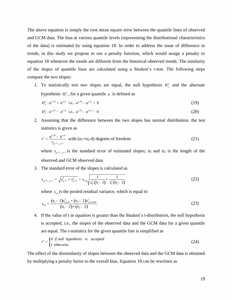
The above equation is simply the root mean square error between the quantile lines of observed
and GCM data. The bias at various quantile levels (representing the distributional characteristics
of the data) is estimated by using equation 18. In order to address the issue of difference in
trends, in this study we propose to use a penalty function, which would assign a penalty to
equation 18 whenever the trends are different from the historical observed trends. The similarity
of the slopes of quantile lines are calculated using a Student’s t-test. The following steps
compare the two slopes:
1. To statistically test two slopes are equal, the null hypothesis oH a and the alternate
hypothesis 1H a , for a given quantile a is defined as
, , ,H ,: . ., 0H G G
oH a a i e a aa a a a a= - = (19)
, , ,H ,
1 : . ., 0H G GH a a i e a aa a a a a¹ - ¹ (20)
2. Assuming that the difference between the two slopes has normal distribution, the test
statistics is given as
, ,
, ,
H G
H G
a a
a at
s a a
a aa
-
-= with (n1+n2-4) degrees of freedom (21)
where , ,H Ga as a a-
is the standard error of estimated slopes; n1 and n2 is the length of the
observed and GCM observed data
3. The standard error of the slopes is calculated as
( ) ( ), , , ,
2 2
2 2
1 2
1 1
1 1H G H H resa a a a
H G
s s s ss n s n
a a a a-= + = +
- - (22)
where ress is the pooled residual variance, which is equal to
( ) ( )
( ) ( )
2 2
1 ,H 2 ,GCM
1 2
2 2
2 2
res res
res
n s n ss
n n
- + -=
- + - (23)
4. If the value of t in equation is greater than the Student’s t-distribution, the null hypothesis
is accepted, i.e., the slopes of the observed data and the GCM data for a given quantile
are equal. The t-statistics for the given quantile line is simplified as
0
1
if null hypothesis is acceptedt
otherwise
aìïï= íïïî
(24)
The effect of the dissimilarity of slopes between the observed data and the GCM data is obtained
by multiplying a penalty factor to the overall bias. Equation 18 can be rewritten as

20
biasSS S (25)
where is the penalty factor based on t-test and is obtained as
1
11 i
k
i
tk
(26)
where k is the total number of quantiles lines used in the study.
The skill scores obtained in the equation 20 are normalized using inter-quantile range of the
observed distribution, which could provide interpretation of scores in terms of the overall spread
of the distribution of observations. The quantile regression based skill scores is given as
QR
H
SSS
IQ= (27)
where IQH is the inter-quantile range of the historical observations.
The best GCMs should have the SQR values close to zero.
3.3 Updating IDF curves under a Changing Climate
The updating procedure for IDF curves is a part of the mathematical models used in the decision
support system of the IDF_CC tool (UserMan: section 1.4). The tool uses an equidistant quantile
matching (EQM) method to update the IDF curves under changing climate conditions (UserMan:
section 3.0). The two main steps of the EQM method are: (i) spatial downscaling of the
maximum precipitation values from the daily global climate models (GCM) data to each of the
sub-daily maximums observed at a station of interest using quantile-mapping functions; and (ii)
temporal downscaling to explicitly capture the changes in the GCM data between the baseline
period and the future period using quantile-mapping function. The flow chart for the EQM
methodology is shown in Fig 4.

21
Figure 4: Equidistance Quantile-Matching Method for generating future IDF curves under
Climate Change
3.3.1 Equidistance Quantile Matching Method
The following section presents the EQM method for updating the IDF curves using IDF_CC
tool. The steps involved in the algorithm are as follows:
(i) Extract sub-daily maximums from the observed data at a given location (i.e., maximums of
5min, 10min, 15min, 1hr, 2hr, 6hr, 12hr, 24hr precipitation data) (UserMan: Section 3.1):
,5min ,10min ,24
1,max 1,max 1,max
,5min ,10min ,24
2,max 2,max 2,max
,5min ,10min ,24
max 3,max 3,max 3,max
,5min ,10min ,24
,max ,max ,max
STN STN STN hr
STN STN STN hr
STN STN STN STN hr
STN STN STN hr
N N N
X X X
X X X
X X X X
X X X
(28)
Historical GCM/RCM Experiment Daily
data Historical Observed
Sub-daily data
Future GCM/RCM
RCP Scenarios – Daily data
Extract Yearly
Maximums Extract Yearly
Maximums Extract Yearly
Maximums
Fit Extreme Value
Distribution (Gumbel)
Fit Extreme Value
Distribution (Gumbel)
Quantile-Mapping
and generate model output
Develop Functional Relationship
Generate Future Sub-daily Extremes
Generate IDF curves for the future
Fit Extreme Value
Distribution (Gumbel)
Quantile-Mapping
and generate model output
Develop Functional Relationship

22
where ,
,max
STN j
iX represents the maximum sub-daily precipitation at a station (STN) for jth
duration in ith year; and N is the total number of years.
(ii) Extract daily (24hr) maximums for the historical base period from the selected GCM model
(UserMan: Section 3.2)
1,max
2,max
max 3,max
,max
GCM
GCM
GCM GCM
GCM
N
X
X
X X
X
(29)
where ,max
GCM
iX represents the maximum daily precipitation from GCM model in ith year and N
is the total number of years (same time span from the historical observed data is used).
(iii) Extract daily maximums from the RCP Scenarios (i.e., RCP26, RCP45, RCP85) for the
selected GCM model (UserMan: Section 3.2):
, 26 , 45 , 85
1,max 1,max 1,max
, 26 , 45 , 85
2,max 2,max 2,max
, 26 , 45 , 85,
3,max 3,max 3,maxmax
, 26 , 45 , 85
N ,max N ,max N ,maxF F F
GCM RCP GCM RCP GCM RCP
GCM RCP GCM RCP GCM RCP
GCM RCP GCM RCP GCM RCPGCM Fut
GCM RCP GCM RCP GCM RCP
X X X
X X X
X X XX
X X X
(30)
where ,
max
GCM FutX represents the maximum daily precipitation for the future scenarios
considered; and NF is the total number of years considered for future time period.
(iv) Fit a probability distribution to the daily maximums from GCM model (each of the sub-
daily maximum series for the observed data and daily maximums for the future scenarios)
(UserMan: Section 3.2):
max
GCM GCM GCMPDF f X (31)
, ,
max
STN STN j STN j
jPDF f X (32)

23
, ,
max
GCM Fut GCM GCM FutPDF f X (33)
where PDF stands for probability distribution function, f() is the function, θ is the parameter
of the fitted distribution
(v) The cumulative probability distribution of the GCM and the sub-daily series are equated to
establish a statistical relationship between them and obtain GCM modeled sub-daily series
max,
GCM
jY using the principle of quantile based mapping. This is spatial downscaling of the data
from the GCM daily maximums to observed sub-daily maximums (UserMan: Section 3.2):
,
max, max
STN GCM GCM STN j
jY CDF invCDF X (34)
where max,
STN
jY is statistically downscaled sub-daily maximum series for jth duration; CDF
stands for cumulative probability distribution function; and invCDF stands for inverse CDF.
(vi) Establish a similar quantile-mapping statistical relationship which models the change
between the current GCM maximums and future GCM maximums. This is temporal
downscaling of the data from the projected GCM simulations of daily maximums to
baseline GCM daily maximums (UserMan: Section 3.2):
, ,
max max
GCM Fut GCM GCM GCM FutY CDF invCDF X (35)
where ,
max
GCM FutY is quantile matching between the baseline period and the projection period.
(vii) Find an appropriate function to relate max,
STN
jY and max
GCMX . Piani et al. (2010) suggested that in
most cases the relation is observed to be linear. It is evident from the Gumbel CDF (eq. 3)
that it results in a linear equation when equating the two CDFs. It is important to note that
there is no guarantee that the use of other distribution functions would result in the similar
linear first order equations (UserMan: Section 3.2).
max, max
STN GCM
jY f X (36)
max, 1 max 1
STN GCM
jY a X b (37)

24
(viii) Find an appropriate function to relate ,
max
GCM FutY and max
GCMX (UserMan: Section 3.2):
,Fut
max max
GCM GCMY f X (38)
,
max 2 max 2
GCM Fut GCMY a X b (39)
(ix) To generate future maximum sub-daily data, combine equations (52) and (54) by replacing
max
GCMX to ,
max
GCM FutY in equation (52) (UserMan: Section 3.2):
,, max 2
max, 1 1
2
GCM futureSTN future
j
X bX a b
a
(40)
(x) Generate IDF curves for the future sub-daily data and compare the same with the
historically observed IDF curves to obtain the change in intensities.
A MATLAB code for updating the IDF curves using the equidistance quantile matching
algorithm is presented in Appendix A.
EXAMPLE: 3.6
The step-by-step procedure followed by the IDF_CC tool for updating IDF curves (UserMan:
Section 3.2 and 3.3):
1. To update the IDF curves use three sets of datasets: (i) daily (24hr) maximums max
GCMX for the
base period from the selected GCM model; (ii) sub-daily maximums from the observed data
at a given location (i.e., maximums of 5min, 10min, 15min, 1hr, 2hr, 6hr, 12hr, 24hr
precipitation data); and (iii) daily maximums from the RCP Scenarios (i.e., RCP26, RCP45,
RCP85) for the selected GCM model. For the case example all the three data sets are in
Appendix C
2. Develop a relationship between the sub-daily historical observed and GCM base period as
well as between the GCM based period and GCM future time period maximum precipitation
data by fitting a probability distribution (see example 3.1)
25
20 40 60 80 100 120 1400
0.1
0.2
0.3
0.4
0.5
0.6
0.7
0.8
0.9
1
Precipitation
F(x
)
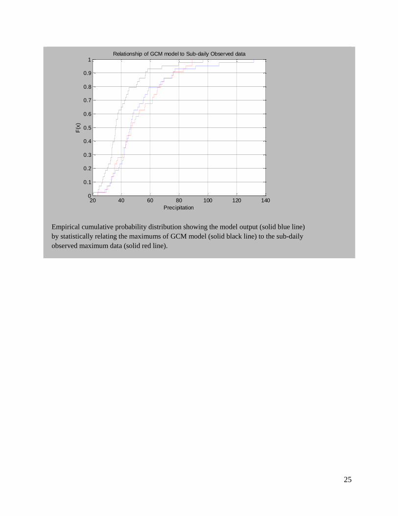
Relationship of GCM model to Sub-daily Observed data
Empirical cumulative probability distribution showing the model output (solid blue line)
by statistically relating the maximums of GCM model (solid black line) to the sub-daily
observed maximum data (solid red line).

26
3. Using equation 34 spatially downscale the data from the GCM daily maximums to observed
sub-daily maximums as shown below.
4. Using equation 35 establish the temporal downscaling of the data from the projected GCM
simulations of daily maximum to baseline GCM daily maximums.
0 20 40 60 80 100 1200
0.1
0.2
0.3
0.4
0.5
0.6
0.7
0.8
0.9
1
Precipitation
F(x
)
Relationship of Future GCM Scenario to Current GCM Scenario
Empirical cumulative probability distribution showing the model output (solid blue line)
by statistically relating the maximums of RCP future data (solid black line) to the
maximums of the current period GCM data (solid red line).

27
5. Fit a linear first order equation to relate max,
STN
jY and max
GCMX in equations 37.
max, 1 max 1 max1.756391 17.5867STN GCM GCM
jY a X b X
6. Similarly, find an appropriate function to relate ,
max
GCM FutY and max
GCMX in equations 39.
,
max 2 max 2 max0.995552 0.077941GCM Fut GCM GCMY a X b X
7. Combine steps 5 and 6 to obtain the future generated data at London station as
, ,, max 2 max
max, 1 1
2
0.0779411.756391 17.5867
0.995552
GCM future GCM futureSTN future
j
X b XX a b
a
8. Generate IDF curves for the future sub-daily data
London
Scenario Change in % to historical
Minutes Historical RCP-26 RCP-45 RCP-85 RCP-26 RCP-45 RCP-85
5 109.5 129.0 135.6 155.8 17.80% 23.86% 42.30%
10 79.2 94.5 99.7 115.6 19.34% 25.93% 45.97%
15 63.6 75.8 79.9 92.5 19.12% 25.63% 45.45%
30 41.1 49.4 52.2 60.9 20.28% 27.19% 48.21%
60 24.5 30.1 31.9 37.7 22.70% 30.43% 53.96%
120 14.8 18.1 19.2 22.7 22.57% 30.25% 53.65%
360 6.1 7.2 7.5 8.6 17.36% 23.27% 41.26%
720 3.6 4.2 4.4 5.0 16.28% 21.83% 38.70%
1440 2.1 2.5 2.7 3.1 19.64% 26.34% 46.70%

28
4. Summary and Conclusion
This document presents the technical reference manual for the Computerized IDF_CC tool for
the Development of Intensity-Duration-Frequency-Curves Under a Changing Climate. The tool
uses a sophisticated although very efficient methodology that incorporates changes in the
distributional characteristics of GCM models between the baseline period and the future period.
The mathematical models and procedures used within the IDF_CC tool include: (i) Statistical
analysis algorithm, which includes fitting Gumbel probability distribution function using method
of moments and spatial interpolation of GCM data using inverse distance method; (ii) GCM
selection using quantile regression skill score; and (iii) IDF updating algorithm based on
equidistance quantile matching method. The document also presents the step-by-step guide for
the implementation of all the mathematical models and procedures.
The IDF_CC tool’s website (www.idf-cc-uwo.com) should be regularly visited for the latest
updates of the IDF_CC tool, new functionalities and updated documentation.
References
Allan RP, Soden BJ (2008) Atmospheric warming and the amplification of precipitation
extremes. Science 321: 1480–1484.
Barnett DN, Brown SJ, Murphy JM, Sexton DMH, Webb MJ (2006) Quantifying uncertainty in
changes in extreme event frequency in response to doubled CO2 using a large ensemble of
GCM simulations. Climate Dynamics 26(5): 489–511, DOI: 10.1007/S00382-005-0097-1.
CSA (Canadian Standards Association). (2012). TECHNICAL GUIDE: Development,
interpretation, and use of rainfall intensity-duration-frequency (IDF) information: Guideline
for Canadian water resources practitioners. Mississauga: Canadian Standards Association.

29
Hassanzadeh E, Nazemi A, Elshorbagy, A. (2013) Quantile-Based Downscaling of Precipitation
using Genetic Programming: Application to IDF Curves in the City of Saskatoon. J. Hydrol.
Eng., 10.1061/(ASCE)HE.1943-5584.0000854
Hog WD, Carr DA, Routledge B (1989) Rainfall Intensity-Duration-Frequency values for
Canadian locations. Downsview; Ontario; Environment Canada; Atmospheric Environment
Service.
Kao SC, Ganguly AR (2011). Intensity, duration, and frequency of precipitation extremes under
21st-century warming scenarios. Journal of Geophysical Research, 116(D16), D16119.
doi:10.1029/2010JD015529
Kharin VV, Zwiers FW, Zhang X, Hegerl G (2007) Changes in temperature and precipitation
extremes in the IPCC ensemble of global coupled model simulations. J Climate 20: 1519-
1444
Li H, Sheffield J, Wood EF (2010) Bias correction of monthly precipitation and temperature
fields from Intergovernmental Panel on Climate Change AR4 models using equidistant
quantile matching. Journal of Geophysical Research, 115(D10), D10101.
doi:10.1029/2009JD012882
Mailhot A, Duchesne S, Caya D, Talbot G (2007). Assessment of future change in intensity-
duration-frequency (IDF) curves for Southern Quebec using the Canadian Regional Climate
Model (CRCM). Journal of Hydrology, 347: 197–210. doi:10.1016/j.jhydrol.2007.09.019
MATLAB version 7.12.0. Natick, Massachusetts: The MathWorks Inc., April 8, 2011.
Milly PCD, Julio Betancourt, Malin Falkenmark, Robert M Hirsch, Zbigniew W Kundzewicz,
Dennis P Lettenmaier, Ronald J Stouffer (2008) Stationarity Is Dead: Whither Water
Management?, Science, 319 (5863), 573-574. [DOI:10.1126/science.1151915]

30
Mirhosseini G, Srivastava P, Stefanova L (2012). The impact of climate change on rainfall
Intensity–Duration–Frequency (IDF) curves in Alabama. Regional Environmental Change,
13(S1), 25–33. doi:10.1007/s10113-012-0375-5
Millington N, Samiran D, Simonovic SP (2011). The comparison of GEV, Log-Pearson Type-3
and Gumbel Distribution in the Upper Thames River Watershed under Global Climate
Models. Water Resources Research Report no. 077, Facility for Intelligent Decision
Support, Department of Civil and Environmental Engineering, London, Ontario, Canada, 54
pages. ISSN: (print) 1931-3200; (online) 1919-3219.
Nguyen VTV, Nguyen TD, Cung A (2007) A statistical approach to downscaling of sub-daily
extreme rainfall processes for climate-related impact studies in urban areas. Water Science
& Technology: Water Supply, 7(2), 183. doi:10.2166/ws.2007.053
Peck A, Prodanovic P, Simonovic SP. (2012). Rainfall Intensity Duration Frequency Curves
Under Climate Change: City of London, Ontario, Canada. Canadian Water Resources
Journal, 37(3), 177–189. doi:10.4296/cwrj2011-935
Piani C, Weedon GP, Best M, Gomes SM, Viterbo P, Hagemann S, Haerter JO. (2010).
Statistical bias correction of global simulated daily precipitation and temperature for the
application of hydrological models. Journal of Hydrology, 395(3-4), 199–215.
doi:10.1016/j.jhydrol.2010.10.024
Simonovic SP, Vucetic D (2012) Updated IDF curves for London, Hamilton, Moncton,
Fredericton and Winnipeg for use with MRAT Project, Report prepared for the Insurance
Bureau of Canada, Institute for Catastrophic Loss Reduction, Toronto, Canada, 94 pages.
Simonovic SP, Vucetic D (2013) Updated IDF curves for Bathurst, Coquitlam, St, John’s and
Halifax for use with MRAT Project, Report prepared for the Insurance Bureau of Canada,
Institute for Catastrophic Loss Reduction, Toronto, Canada, 54 pages.

31
Solaiman TA, Simonovic SP (2011) Development of Probability Based Intensity-Duration-
Frequency Curves under Climate Change. Water Resources Research Report no. 072,
Facility for Intelligent Decision Support, Department of Civil and Environmental
Engineering, London, Ontario, Canada, 89 pages. ISBN: (print) 978-0-7714-2893-7;
(online) 978-0-7714-2900-2.
Solaiman TA, Simonovic SP (2010) National centers for environmental prediction -national
center for atmospheric research (NCEP-NCAR) reanalyses data for hydrologic modelling
on a basin scale (2010) Canadian Journal of Civil Engineering, 37 (4), pp. 611-623.
Solaiman TA, King LM, Simonovic SP (2011) Extreme precipitation vulnerability in the Upper
Thames River basin: uncertainty in climate model projections. Int. J. Climatol., 31: 2350–
2364. doi: 10.1002/joc.2244
Srivastav RK, Andre Schardong, Slobodan P. Simonovic (2014), Equidistance Quantile
Matching Method for Updating IDF Curves under Climate Change, Water Resources
Management, doi: 10.1007/s11269-014-0626-y
Srivastav RK, Slobodan P. Simonovic (2014), Quantile Regression for Selection of GCMs,
Climate Dynamics (under review)
Sugahara Shigetoshi, Rocha RP, Silveira R (2009) Non-stationary frequency analysis of extreme
daily rainfall in Sao Paulo , Brazil, 29, 1339–1349. doi:10.1002/joc.
Taylor KE, Stouffer RJ, Meehl GA (2012) An overview of CMIP5 and the experiment design.
Bull Am Met Soc 93(4):485–498. doi:10.1175/bams-d-11-00094.1
Walsh J (2011) Statistical Downscaling, NOAA Climate Services Meeting, 2011.
Wilby RL, Dawson CW (2007) SDSM 4.2 – A decision support tool for the assessment of
regional climate change impacts. Version 4.2 User Manual.

32
Wilcox EM, Donner LJ (2007) The frequency of extreme rain events in satellite rain-rate
estimates and an atmospheric general circulation model. Journal of Climate 20(1): 53–69.
Acknowledgements
The authors would like to acknowledge the financial support by the Canadian Water Network
Project under Evolving Opportunities for Knowledge Application Grant to the third author and
Dan Sandink from ICLR - Institute for Catastrophic Loss Reduction for his support and
assistance with this project.

33
Appendix – A: MATLAB code to update IDF curves
UPDATE IDF CURVES – MATLAB CODE
Contents
Intensity-Duration-Frequency Curves Under Climate Change
Clear Workspace and Command Window
Input Data
FIT Extreme value distribution
Intensity-Duration-Frequency Curves Under Climate Change
% Author: Roshan K. Srivastav
% Method: Equidistance Quantile Matching
% Citation: Roshan K. Srivastav, Andre Schardong, Slobodon P. Simonovic,
% Equidistance Quantile Matching Method for Updating IDF Curves under Climate
% Change, Water Resources Management, 2014
% Doi: 10.1007/s11269-014-0626-y
Clear Workspace and Command Window
clear all
close all
clc
Input Data
% Load Input Data
% Includes: Sub-daily Maximums, GCM base period daily maximum, GCM future
% period daily maximum
load input_data
% Sub-daily Time Interval
subdaily = [5,10,15,30,60,120,360,720,1440];
% Return Period
RT = [2,5,10,25,50,100];
P = 1./RT;
FIT Extreme value distribution
% Fitting Gumbel Distribution
% Negative sign for Gumbel distribution
% Positive is for minimums for evfit
IDF = zeros(size(data_hist,2),length(P));
hist_error = zeros(size(data_hist,2),length(P));

34
future_change1 = zeros(size(data_hist,2),length(P));
future_change2 = zeros(size(data_hist,2),length(P));
IDF_gen = zeros(size(data_hist,2),length(P));
IDF_gen1 = zeros(size(data_hist,2),length(P));
IDF_gen2 = zeros(size(data_hist,2),length(P));
IDF_gen3 = zeros(size(data_hist,2),length(P));
mtrA = zeros(size(data_hist,2), 4);
mtrPar = zeros(size(data_hist,2), 6);
for i = 1:size(data_hist,2)
max_hist_con = data_hist(:,i);
% Fitting Gumbel Distribution
parm_maxfit_hist = evfit(-max_hist_con);
parm_maxfit_gcm = evfit(-max_gcm_con);
parm_maxfit_gcm_fut = evfit(-max_gcm_fut);
mtrPar(i,1) = -parm_maxfit_hist(1); mtrPar(i,2) = parm_maxfit_hist(2);
mtrPar(i,3) = -parm_maxfit_gcm(1); mtrPar(i,4) = parm_maxfit_gcm(2);
mtrPar(i,5) = -parm_maxfit_gcm_fut(1); mtrPar(i,6) = parm_maxfit_gcm_fut(2);
pre_model = evinv(evcdf(-max_gcm_con,parm_maxfit_gcm(1,1),parm_maxfit_gcm(1,2)),...
parm_maxfit_hist(1,1),parm_maxfit_hist(1,2));
pre_model_fut = evinv(evcdf(-
max_gcm_fut,parm_maxfit_gcm_fut(1,1),parm_maxfit_gcm_fut(1,2)),...
parm_maxfit_gcm(1,1),parm_maxfit_gcm(1,2));
pre_model_fut_reverse = evinv(evcdf(-
max_gcm_con,parm_maxfit_gcm(1,1),parm_maxfit_gcm(1,2)),...
parm_maxfit_gcm_fut(1,1),parm_maxfit_gcm_fut(1,2));
post_para = polyfit(max_gcm_con,-pre_model,1);
post_para3 = polyfit(-pre_model_fut_reverse,max_gcm_con,1);
pre_model1 = polyval(post_para,max_gcm_con);
% Not accommodating Future Change
pre_model_fut1 = polyval(post_para,max_gcm_fut);
% Accommodating Future Change
a1 = post_para(1,1);b1 =post_para(1,2);

35
a2 = post_para3(1,1);b2 = post_para3(1,2);
pre_model_fut3 = (a1*((max_gcm_fut-b2)./a2))+b1;
%Historical IDF
IDF(i,:) = -(evinv(P,parm_maxfit_hist(1,1),parm_maxfit_hist(1,2)))*(60/subdaily(i));
parm_maxfit_gcm0 = evfit(-pre_model1);
parm_maxfit_gcm3 = evfit(-pre_model_fut3);
% GCM IDF for Historical Time Period
IDF_gen(i,:) = -(evinv(P,parm_maxfit_gcm0(1,1),parm_maxfit_gcm0(1,2)))*(60/subdaily(i));
% GCM IDF for Equidistant Quantile Mapping Future Time Period
IDF_gen3(i,:) = -
(evinv(P,parm_maxfit_gcm3(1,1),parm_maxfit_gcm3(1,2)))*(60/subdaily(i));
end
% Plot to generate Cumulative Probability Distribution Function
figure
h1= cdfplot(max_gcm_con);
set(h1, 'Color','black')
hold on
h2 = cdfplot(-pre_model);
set(h2, 'Color','blue')
h3 = cdfplot(max_hist_con);
set(h3,'Color','red')
xlabel('Precipitation');
% Plot to generate Cumulative Probability Distribution Function
figure
plot(IDF_gen3','o-')
set(gca,'XTickLabel',{'2';'5';'10';'25';'50';'100'});
title('Updated IDF Curve');
xlabel('Return Period');
ylabel('Intensities');
legend('Duration','Location','NorthWest')

36
Graphical Outputs:

37
Appendix – B: GCMs used in IDF_CC tool
The selected CMIP5 models and their attributes which has all the three emission scenarios
(RCP2.6, RCP4.5 and RCP8.0)
Country Centre
Acronym Model Centre Name
Number of Ensembles
(PPT)
GCM Resolutions
(Lon. vs Lat.)
China BCC bcc_csm1_1 Beijing Climate Center, China Meteorological Administration
1 2.8 x 2.8
China BCC bcc_csm1_1 m Beijing Climate Center, China Meteorological Administration
1
China BNU BNU-ESM College of Global Change and Earth System Science
1 2.8 x 2.8
Canada CCCma CanESM2 Canadian Centre for Climate Modeling and Analysis
5 2.8 x 2.8
USA CCSM CCSM4 National Center of Atmospheric Research
1 1.25 x 0.94
France CNRM CNRM-CM5
Centre National de Recherches Meteorologiques and Centre Europeen de Recherches et de Formation Avancee en Calcul Scientifique
1 1.4 x 1.4
Australia CSIRO3.6 CSIRO-Mk3-6-0
Australian Commonwealth Scientific and Industrial Research Organization in collaboration with the Queensland Climate Change Centre of Excellence
10 1.8 x 1.8
USA CESM CESM1-CAM5 National Center of Atmospheric Research
1 1.25 x 0.94
China LASG-CESS
FGOALS_g2
IAP (Institute of Atmospheric Physics, Chinese Academy of Sciences, Beijing, China) and THU (Tsinghua University)
1 2.55 x 2.48
USA NOAA GFDL
GFDL-CM3
National Oceanic and Atmospheric Administration's Geophysical Fluid Dynamic Laboratory
1 2.5 x 2.0
USA NOAA GFDL
GFDL-ESM2G
National Oceanic and Atmospheric Administration's Geophysical Fluid Dynamic Laboratory
1 2.5 x 2.0
United Kingdom
MOHC HadGEM2-AO Met Office Hadley Centre 1 1.25 x 1.875
United Kingdom
MOHC HadGEM2-ES Met Office Hadley Centre 2 1.25 x 1.875
France IPSL IPSL-CM5A-LR Institut Pierre Simon Laplace 4 3.75 x 1.8
France IPSL IPSL-CM5A-MR Institut Pierre Simon Laplace 4 3.75 x 1.8
Japan MIROC MIROC5 Japan Agency for Marine-Earth Science and Technology
3 1.4 x 1.41
Japan MIROC MIROC-ESM Japan Agency for Marine-Earth Science and Technology
1 2.8 x 2.8

38
Country Centre
Acronym Model Centre Name
Number of Ensembles
(PPT)
GCM Resolutions
(Lon. vs Lat.)
Japan MIROC MIROC-ESM-CHEM Japan Agency for Marine-Earth Science and Technology
1 2.8 x 2.8
Germany MPI-M MPI-ESM-LR Max Planck Institute for Meteorology
3 1.88 x 1.87
Germany MPI-M MPI-ESM-MR Max Planck Institute for Meteorology
3 1.88 x 1.87
Japan MRI MRI-CGCM3 Meteorological Research Institute 1 1.1 x 1.1
Norway NOR NorESM1-M Norwegian Climate Center 3 2.5 x 1.9
39
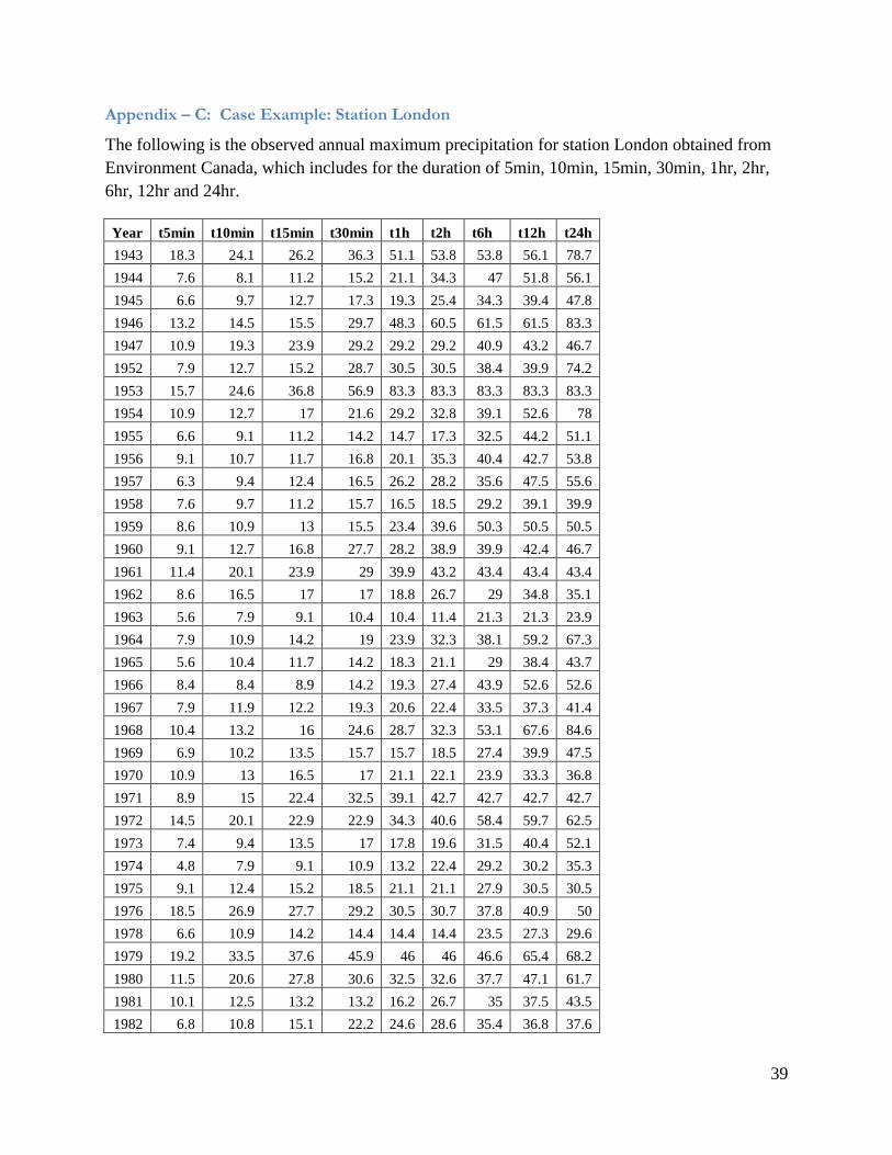
Appendix – C: Case Example: Station London
The following is the observed annual maximum precipitation for station London obtained from
Environment Canada, which includes for the duration of 5min, 10min, 15min, 30min, 1hr, 2hr,
6hr, 12hr and 24hr.
Year t5min t10min t15min t30min t1h t2h t6h t12h t24h
1943 18.3 24.1 26.2 36.3 51.1 53.8 53.8 56.1 78.7
1944 7.6 8.1 11.2 15.2 21.1 34.3 47 51.8 56.1
1945 6.6 9.7 12.7 17.3 19.3 25.4 34.3 39.4 47.8
1946 13.2 14.5 15.5 29.7 48.3 60.5 61.5 61.5 83.3
1947 10.9 19.3 23.9 29.2 29.2 29.2 40.9 43.2 46.7
1952 7.9 12.7 15.2 28.7 30.5 30.5 38.4 39.9 74.2
1953 15.7 24.6 36.8 56.9 83.3 83.3 83.3 83.3 83.3
1954 10.9 12.7 17 21.6 29.2 32.8 39.1 52.6 78
1955 6.6 9.1 11.2 14.2 14.7 17.3 32.5 44.2 51.1
1956 9.1 10.7 11.7 16.8 20.1 35.3 40.4 42.7 53.8
1957 6.3 9.4 12.4 16.5 26.2 28.2 35.6 47.5 55.6
1958 7.6 9.7 11.2 15.7 16.5 18.5 29.2 39.1 39.9
1959 8.6 10.9 13 15.5 23.4 39.6 50.3 50.5 50.5
1960 9.1 12.7 16.8 27.7 28.2 38.9 39.9 42.4 46.7
1961 11.4 20.1 23.9 29 39.9 43.2 43.4 43.4 43.4
1962 8.6 16.5 17 17 18.8 26.7 29 34.8 35.1
1963 5.6 7.9 9.1 10.4 10.4 11.4 21.3 21.3 23.9
1964 7.9 10.9 14.2 19 23.9 32.3 38.1 59.2 67.3
1965 5.6 10.4 11.7 14.2 18.3 21.1 29 38.4 43.7
1966 8.4 8.4 8.9 14.2 19.3 27.4 43.9 52.6 52.6
1967 7.9 11.9 12.2 19.3 20.6 22.4 33.5 37.3 41.4
1968 10.4 13.2 16 24.6 28.7 32.3 53.1 67.6 84.6
1969 6.9 10.2 13.5 15.7 15.7 18.5 27.4 39.9 47.5
1970 10.9 13 16.5 17 21.1 22.1 23.9 33.3 36.8
1971 8.9 15 22.4 32.5 39.1 42.7 42.7 42.7 42.7
1972 14.5 20.1 22.9 22.9 34.3 40.6 58.4 59.7 62.5
1973 7.4 9.4 13.5 17 17.8 19.6 31.5 40.4 52.1
1974 4.8 7.9 9.1 10.9 13.2 22.4 29.2 30.2 35.3
1975 9.1 12.4 15.2 18.5 21.1 21.1 27.9 30.5 30.5
1976 18.5 26.9 27.7 29.2 30.5 30.7 37.8 40.9 50
1978 6.6 10.9 14.2 14.4 14.4 14.4 23.5 27.3 29.6
1979 19.2 33.5 37.6 45.9 46 46 46.6 65.4 68.2
1980 11.5 20.6 27.8 30.6 32.5 32.6 37.7 47.1 61.7
1981 10.1 12.5 13.2 13.2 16.2 26.7 35 37.5 43.5
1982 6.8 10.8 15.1 22.2 24.6 28.6 35.4 36.8 37.6

40
1983 13.5 23.4 29.5 37.6 41.1 41.1 47 55.8 64.4
1984 9.8 10.6 14.5 27.4 27.8 43.5 50.8 56 69.7
1985 8.3 10.9 13.7 22.8 29 35.1 43.2 56.8 65
1986 12.4 22.7 24.2 24.5 30.6 42.2 43.8 49.7 89.1
1987 6.7 9.4 11 13.2 14.3 17.7 27.2 44.5 56.5
1988 7.9 11.2 15.5 18.2 18.3 26.9 33 41.9 61.6
1989 8.7 10.9 13.5 23.3 25.7 25.8 25.8 34 34.8
1990 11.9 16.7 18.7 30.4 35.1 37.9 41.6 54.1 75.5
1991 9.7 11.6 13.9 17.5 20.6 22 28.1 32.2 32.2
1992 6.5 11.5 15.9 20.9 35 45.2 51.8 58.6 76.3
1993 9.4 14.3 15.1 19.1 21.9 25 28.5 30.7 49.2
1994 7.5 11.3 12.1 16.8 20.6 33.2 38.9 40.3 46.5
1995 8.2 11.3 12.6 15.8 21.8 28 37.8 45 56.1
1996 9.4 15.8 17.9 26.1 39.2 68.1 82.7 83.5 89
1997 10.6 17 19.6 21.8 21.8 24.8 31.1 33.9 33.9
1998 12.6 14.7 15.8 17.6 20.4 20.4 20.4 -99.9 33
1999 7.3 11.2 11.8 12.7 13.3 19 25.9 26.1 32.9
2000 11.5 15.3 17.6 23 30.6 40.6 -99.9 -99.9 82.8
2001 6.3 7.9 10.6 13.2 13.4 14 24 35 41.2
2003 10 18.4 23.2 26.2 26.2 27.8 31.2 40.8 40.8
2004 15 23.6 27.2 29.4 29.4 29.6 45.4 47 47
2005 9 12.6 15.4 19.8 19.8 24 35.6 37 45.6
The spatially interpolated GCM data for the base period at station London is provided in the
following table
Year Base Period
1943 34.63
1944 34.43
1945 34.28
1946 51.60
1947 32.92
1948 50.02
1949 37.82
1950 32.21
1951 42.36
1952 43.10
1953 38.08
1954 28.46
1955 35.80
1956 26.83
1957 33.12

41
1958 44.76
1959 37.43
1960 54.24
1961 38.72
1962 27.76
1963 27.76
1964 34.52
1965 40.38
1966 34.68
1967 33.76
1968 34.89
1969 45.03
1970 41.13
1971 46.69
1972 35.53
1973 59.03
1974 31.32
1975 29.93
1976 49.26
1977 35.04
1978 44.41
1979 21.62
1980 20.91
1981 31.51
1982 46.85
1983 50.55
1984 41.23
1985 46.08
1986 34.22
1987 42.09
1988 27.97
1989 39.61
1990 54.70
1991 40.46
1992 42.18
1993 54.02
1994 45.39
1995 42.75
1996 35.68
1997 43.81
1998 69.71
1999 39.77
2000 55.65

42
2001 48.19
2002 65.94
2003 37.12
2004 59.16
2005 36.84
The spatially interpolated future emission scenarios (RCP) data at station London is provided in
the following table
Year RCP 2.6 RCP 4.5 RCP 8.5
2006 45.1622 57.745 31.74
2007 48.53682 31.256 53.89
2008 36.85236 40.106 28.71
2009 41.17063 36.583 49.78
2010 40.93406 40.890 49.84
2011 55.58957 42.050 42.66
2012 39.65082 50.934 20.78
2013 29.20486 43.575 30.35
2014 37.10033 43.321 40.98
2015 70.95828 32.892 34.43
2016 33.26686 39.338 46.30
2017 36.90782 39.642 49.66
2018 41.95582 42.081 48.48
2019 39.66497 35.705 54.66
2020 43.60934 30.119 46.94
2021 37.86769 33.413 63.94
2022 49.84933 61.525 37.11
2023 52.10321 38.091 57.37
2024 20.86538 25.500 54.61
2025 41.31501 47.266 54.76
2026 33.08702 36.387 43.58
2027 56.08242 51.171 34.66
2028 64.24603 37.642 46.91
2029 56.54352 39.311 36.12
2030 22.96999 47.543 62.53
2031 34.20818 27.236 38.94
2032 53.67458 44.221 40.46
2033 42.72022 49.044 30.89
2034 44.48209 50.753 61.28
2035 39.70259 44.216 45.55
2036 47.27356 41.163 31.28
2037 76.85988 51.525 43.96

43
2038 62.32694 35.653 30.67
2039 44.68479 55.899 33.42
2040 30.78315 47.668 34.24
2041 39.6506 33.138 36.26
2042 41.13341 44.204 37.19
2043 53.4278 43.447 42.24
2044 36.09163 45.177 38.98
2045 29.66711 57.015 67.19
2046 46.40982 60.701 27.25
2047 55.65701 35.222 76.35
2048 40.69816 44.762 55.70
2049 32.88202 37.870 47.44
2050 35.28659 42.718 57.42
2051 58.92524 45.856 37.17
2052 39.22736 50.030 23.40
2053 35.62452 36.009 45.83
2054 47.08407 45.170 43.28
2055 39.72457 35.343 68.28
2056 29.99022 65.162 31.88
2057 43.4929 30.265 27.26
2058 40.0485 32.709 28.19
2059 82.33642 58.606 29.83
2060 56.48761 82.828 55.47
2061 39.89108 48.574 87.36
2062 34.73032 49.215 45.34
2063 39.21705 27.270 41.92
2064 41.5507 93.814 48.55
2065 40.69927 43.739 40.05
2066 38.54787 62.448 37.81
2067 49.2338 30.695 43.22
2068 41.62116 36.980 57.70
2069 34.6986 45.649 56.08
2070 42.10195 72.245 37.55
2071 25.86632 37.988 55.51
2072 38.77699 48.252 43.66
2073 28.1056 44.555 58.32
2074 67.61863 48.759 28.67
2075 36.82727 59.058 46.06
2076 40.1619 41.898 58.50
2077 46.96967 29.850 35.47
2078 34.25636 39.844 35.05
2079 33.87169 41.633 61.95
2080 28.23784 57.564 72.76

44
2081 45.60183 47.244 58.74
2082 54.25554 37.537 72.05
2083 22.0559 40.981 44.21
2084 39.41858 34.337 61.29
2085 42.28307 47.888 29.63
2086 35.81371 57.430 40.09
2087 28.65652 66.901 58.96
2088 34.92259 37.336 42.13
2089 44.16422 46.244 64.23
2090 39.4304 39.608 25.54
2091 33.29272 30.975 36.00
2092 40.11237 34.809 65.06
2093 28.79 60.399 40.09
2094 47.08903 54.277 51.39
2095 26.71159 41.710 40.47
2096 37.41567 50.913 41.95
2097 48.71734 41.359 65.01
2098 36.83587 35.281 58.88
2099 64.10738 56.363 93.11
2100 48.30834 36.481 49.46

45
Appendix – E: Journal paper on Quantile Regression for selection of GCMs (Under Review)

1
A New Skill Score for Selection of Climate Models using Quantile Regression 1
Roshan K. Srivastav and Slobodan P. Simonovic, Department of Civil and Environmental 2
Engineering, Western University, Canada. 3
4
Key Points 5
• The skill score based on distributional and bias characteristics 6
• Technique that captures trends present in the data 7
• Skill scores can be directly converted to weights of the ensembles 8
9
ABSTRACT 10
A number of General Circulation Models (GCM) has been developed based on several factors 11
representing the dynamics within the earth’s atmosphere and its interactions with the land, 12
cryosphere and oceans. A good GCM model should be able to mimic the distributional 13
characteristics as well as trends (evolution of process) present in the regional-scale observed 14
data. Not all the GCM’s (due to coarse grid scale) will be able to represent the local conditions 15
(point features) with same accuracy, since each of them considers slightly different feedback 16
interactions. The selection and/or ranking of GCMs are/is vital in reducing modeling uncertainty 17
and computational time for decision making. This study proposes a new skill score based on 18
quantile regression (QRSS) for comparing the climate models. The proposed technique 19
incorporates both the distributional characteristics and the trends present in the data. The QRSS 20
combines (i) the quantiles which represent the distribution of the variables and (ii) the parameters 21
of the first-order quantile regressions representing the trends present in the variables. In this 22
study, 23 GCMs are used to rank the climate models for 52 stations located in the Grand River 23
Basin, Canada. The ranking process is based on four atmospheric variables: precipitation, 24
maximum temperature, minimum temperature and near-surface temperature. It is observed that 25
the proposed method is skillful in capturing both the distributional and trend characteristics 26
present in the datasets. The performance of the GCM models is the best for minimum 27
temperature and surface temperature, followed by maximum temperature and worst for 28
precipitation. In the case of temperature variables it is possible to select a single best GCM. 29
However, the same finding is not applicable for precipitation. Many different GCM models are 30
found to provide the best estimate of precipitation. The proposed method offers a valuable 31

2
contribution to hydro-climatology in (i) reducing uncertainty in selection of GCM models and 1
(b) providing for weighting the GCM models in ensemble analyses. 2
3
Index Terms: Skill score, Climate Models, Quantile Regression, GCM 4
5
1.0 Introduction 6
General Circulation Models (GCM) describe the dynamics within the Earth’s atmosphere and are 7
used to understand the current and future climatic conditions. With help of GCMs it is possible 8
to assess the effects of climate change on various earth systems such as hydrology, ecology, 9
physical and biochemical processes and human health. The Intergovernmental Panel for Climate 10
Change (IPCC) and other leading international organizations, who are actively addressing the 11
impacts of climate change on Earth system and humans, have been relying on the conclusions 12
drawn from the GCM models. A number of GCM models has been developed, which are based 13
on (i) land-ocean-atmospheric coupling; (ii) greenhouse gas emissions; and (iii) different initial 14
conditions representing the variations within the climate system. The GCMs simulate the change 15
in atmospheric variables on courser grid scales (temporal and spatial) and are expected to mimic 16
the dynamics of regional-scale climate conditions well. 17
18
Many hydro-climatic studies have indicated that the uncertainty arising from the choice of GCM 19
is significant when compared to other sources of uncertainty (Wilby and Harris 2006; Suraje and 20
Hulme 2007; Kendon et al. 2008; Kay et al. 2009; Prudhomme and Davies 2009; Teutschbein et 21
al. 2011; Woldemeskel et al. 2012). It also observed that not all the GCMs will be able to 22
replicate the regional-scale dynamics well, since each of them simulates the atmospheric 23
feedback processes differently. The use of all available GCMs for the hydroclimatic studies 24
could be computationally very demanding. In order to reduce the uncertainty due to choice of the 25
GCM the performance metrics, or the skill scores were proposed (Giorgi and Mearns 2002; 26
Murphy et al. 2004; Dessai et al. 2005; Wilby and Harris 2006; Perkins et al. 2007; Gleckler et 27
al. 2008; Johnson and Sharma 2009; Yokoi et al. 2011). These performance metrics or skill 28
scores are used to rank the GCMs according to their performance of or assign weights to the 29
GCMs that may be used in an ensemble, which in-turn assists in the reduction of uncertainty. 30
31

3
Giorgi and Mearns (2002) proposed the reliability ensemble average (REA) to assess the 1
dependability of GCMs. The REA has two components, named as model performance measure 2
and model convergence measure. The model performance measure explains the bias, or error, in 3
the GCM simulations (which is the difference between the model output and the historical 4
observed data). The model convergence is based on the performance of a GCM forcing 5
experiment when compared to the multi-model ensemble average (Dessai et al. 2005). The REA 6
was applied for two atmospheric variables: mean seasonal temperature and precipitation. Later 7
Dessai et al. (2005) extended a similar two criteria approach but with a different skill score. They 8
proposed skill score based on the ratio of absolute average of the observed data to the root mean 9
square error between the model and the observed data. They applied their proposed skill score to 10
the same datasets as Giorgi and Mearns (2002). Johnson and Sharma (2009) proposed a model 11
convergence measure based on the coefficient of variation (CV) to rank the GCM models and 12
named it as variable convergence score (VCS). This method considers both base-period and 13
future period GCM simulations into the VCS. Eight surface and atmospheric variables and two 14
scenarios were selected from Australia to study the VCS. 15
16
Murhy et al. (2004) developed Climate Prediction Index (CPI) to weight the GCM models based 17
on the relative likelihood of the model to predict the observed data. The CPI combines the 18
weighted mean square error between the model output and the historical observed data and the 19
spatial average of the simulated internal variance. They used 32 observed atmospheric variables 20
in the climate prediction index (Murhy et al. 2004). Later Wilby and Harris (2006) refined the 21
CPI and developed a new impact relevant climate prediction index (IRCPI). The IRCPI do not 22
consider any statistics related to ensembles or model convergence instead compares directly each 23
GCM output and its ability to mimic the historical observed characteristics. The CPI index was 24
used to assess the performance of the GCM models in downscaling precipitation and potential 25
evapotranspiration in River Thames basin, UK. 26
27
Perkins et al. (2007) developed a skill score based on probability density function (PDF) to rank 28
the GCM models. In this method the PDF’s of the model output and the historical observed data 29
are matched and the degree of matching is considered as the skill score. The daily simulations of 30
precipitation, maximum temperature and minimum temperature from Australia are used in their 31

4
work. Gleckler et al. (2008) proposed skill measures based on relative error and developed an 1
exploratory model variability index (MVI) in order to weight each of the GCM models. They 2
have considered 22 surface and atmospheric variables in evaluating the skill measures. Recently 3
Yokoi et al. (2011) proposed a clustering analysis to group the performance metrics instead of 4
using individual metrics. Clustering techniques such as k-means and Ward method were applied 5
to form groups from 43 metrics. 6
7
The aim of any skill score or performance metric is to assess the degree to which the model data 8
and the historical observed data match or differ from each other. The important characteristics of 9
the model and observed datasets to be considered include: (i) error statistics; (ii) distribution of 10
the data; and (iii) time evolution of the process. The error statistics explain the average distance 11
between the model and the observed data. The distributional characteristics of the data will 12
provide the understanding of the degree of variations in the magnitude of a variable. Both these 13
statistics are independent of the process time evolution. However, in addition to the above 14
statistics, the changes in magnitude with time also play an important role in simulating the 15
dynamics of the climate system. Therefore, the GCM models should not only mimic the 16
distributional statistics, or minimize the bias, but also be able to match the trends present in the 17
historical observed data. 18
19
Most of the metrics proposed in the literature use one form or the other of error statistics or 20
distribution of the data to rank the GCM models. To the best of our knowledge, there is no skill 21
score method which explicitly incorporates trends in the selection of the GCM models. In this 22
paper a new skill score based on the quantile regression (QRSS) is proposed to assess the 23
performance of the GCM models. The proposed QRSS approach includes two main components: 24
(i) the quantiles representing the distribution of the data; and (ii) the quantile regression lines that 25
describe the trends and heteroscedasticity across the quantiles. The QRSS has the ability to 26
capture: (i) the distributional characteristics; (ii) the error statistics; and (iii) the most importantly 27
compares the trends (i.e. evolution of process with time) between GCM simulated and observed 28
time series. 29
30

5
The remainder of the paper is organized as follows. In Section 2, the details of the proposed 1
quantile regression based skill score are presented. The details of a case study and GCM models 2
used are presented in Section 3. The performance of each of the GCM models based on the 3
QRSS is presented in Section 4. Finally, the summary and conclusions of the present study are 4
outlined in Section 5. 5
6
2.0 METHODOLOGY 7
First we present a brief description of quantile regression and its mathematical formulation. 8
Following this we present the methodology to calculate QRSS for ranking the GCM models. 9
10
2.1 The Quantile Regression 11
Quantile regression (QR) belongs to a class of regression analysis, which unlike the traditional 12
linear regression (a) is flexible in dealing with non-normally distributed errors, (b) robust to 13
outliers, and (c) has the ability to detect heterogeneity. The linear regression models estimate the 14
dependent variable based on the conditional mean for a given set of independent variables; while 15
the quantile regression models estimate the conditional quantile functions of a dependent 16
variable, for a given set of independent variables. Quantile regression was introduced in 17
econometrics by Koenker and Bassett (1978). Since then, the quantile regression has been used 18
in various applications because of its advantage over traditional linear regression. The use of 19
quantile regression in hydro-climatology has been very limited, however it started gaining 20
popularity in recent years. Most of the studies in hydro-climatology adopted the quantile 21
regression approach for downscaling (Burger et al. 2012; Tareghian and Rasmussen 2013), 22
forecasting (Esfahani and Friedel 2014) and trend analyses (Franzke 2013; Kim and Jain 2013). 23
To the best of our knowledge, no studies have been reported that used the quantile regression for 24
assessing or comparing the GCM model outputs. The main objective of this paper is to present a 25
new skill score method based on the use of quantile regression for ranking GCM models. 26
27
The mathematical formulation of quantile regression is presented below (after Koenker and 28
Bassett, 1978) 29
(i) Let the weather variable be represented by X and denoted by 30

6
{ }1 2, ,...., tX x x x= (1) 1
where t is index for time and can be denoted by 2
{ }1,2,3, ,t T= ⋯ (2) 3
(ii) For a given thα quantile, the linear model is expressed as 4
1,....,i i i
x t e i Tαβ′= + = (3) 5
where x is the weather variable; t′ is transpose of variable time; α is the quantile; T is 6
the length of total time period; e is residual error; and αβ is the parameter at α defined 7
below. 8
(iii) Let ( )Q X tα represent the relationship between the weather variable and time in eq 9
(3)and be expressed as 10
( )Q X t tα αβ′= (4) 11
(iv) The parameter αβ at αth
quantile can be written as 12
13
( )1
ˆ a rg m inn
i i
i
f x tα αβ
β β=
′= −∑ (5) 14
15
where the function ( )f uα for any value u is given as 16
17
( ) ( )( 1) 0
0
u if uf u
u if uα
αα− <
= ≥ (6) 18
(v) The estimate of the regression quantile can be expressed as 19
20
( ) ˆQ̂ X t tα αβ′= (7) 21
22
The function for ˆαβ is monotonic and hence would result in an optimal solution. The parameter 23
ˆαβ can be solved using linear programming. More details on the quantile regression can be found 24

7
in Koenker (2005). The following paragraph describes the use of quantile regression in obtaining 1
the GCM skills. 2
3
2.2 The Quantile Regression-based Skill Score Method (QRSS) 4
The quantile regression based skill score method (QRSS) proposed in this study uses the 5
quantiles to cover the distribution of the data and the coefficients of the linear quantile function 6
to capture the trends and the biases (distance or error) in the GCM output and historical observed 7
data. The QRSS includes two main components: (i) the dissimilarity skill score (DSS) i.e., how 8
close are the historical and GCM quantile regression lines; and (ii) the trend skill score (TSS) 9
i.e., to what extent the slopes of historical and GCM quantile regression lines are different from 10
each other. The following is the description of the QRSS calculation. 11
12
Let the historical observed data HX , the GCM model data GX and the quantiles A be represented 13
respectively as 14
15
{ }1 2, ,....,H H H H
tX x x x= (8) 16
{ }1 2, ,....,G G G G
tX x x x= (9) 17
{ }1 2, ,...., nα α αΑ = (10) 18
19
where the superscript H and G represents historical and GCM model data, respectively; n is the 20
number of quantiles considered. 21
22
For a given quantile level α, the linear quantile function is given as 23
24
, , ,ˆ 1,2,3, ,H H HX a t b t Tα α α= + ∀ = … (11) 25
, , ,ˆ 1,2,3, ,G G GX a t b t Tα α α= + ∀ = … (12) 26
27
where a and b represent the coefficients of linear quantile function as slope and intercept, 28
respectively at αth
quantile; t is the time variable; and T is the total time period. 29
30

8
2.3 Dissimilarity Skill Score (DSS) 1
It is expected that the GCM models should be able to generate the variable values close to the 2
historical observed data. However, the models are not perfect and exhibit systematic bias and 3
variability in the generation process. The dissimilarity skill score ( biasSα ) measures the degree of 4
bias at each quantile level α between the GCM model data set and the observed data set and is 5
given as: 6
7
2,
,1
ˆ11
ˆ
GTi
bias Hi
XS
T X
αα
α=
= −
∑ (13) 8
9
The above equation is simply the relative root mean square error. The above equation (13) is not 10
desirable in following two cases. 11
First, the main objective of the proposed QRSS is to assess the time evolution process of the 12
variable considered in addition to the distributional or bias characteristics of the datasets. In this 13
study the time evolution of process in a given atmospheric variable is represented by the trend of 14
the quantile lines (slope of the line). Ideally if the GCMs are able to mimic the historical 15
processes exactly, then the trends present in the GCM outputs should be equal to the trends 16
present in the historical observed data (i.e., the slope of the GCM generated and historical 17
quantile regression lines should be equal). However, the GCMs are imperfect and are unable to 18
capture the complete underlying process of the observed data. These imperfections in modeling 19
outputs result into two issues associated with GCM: (1) bias in the GCM output; and (2) 20
difference in the time evolution process between the GCM generated and the observed data. The 21
bias in the GCM data can be easily adjusted or corrected (if required) and hence these 22
imperfections are managable. The trends in the GCM outputs and historical outputs should be 23
similar, in spite of the bias, otherwise the GCM outputs may be undesirable. The model outputs 24
can be corrected for the bias but cannot be easily corrected for difference in trends. Even if it can 25
be corrected for the base time period, it would be very difficult to correct the GCM outputs for 26
the future time period. Hence it is important that GCMs should be able to reproduce the trends 27
present in the historical data. The QRSS method tries to address this issue by ranking the GCM 28

9
not only based on bias and distributions but also based on trends present in GCM data and 1
historical data. 2
3
Second, although the bias could be small, the trend lines of the GCM output and historical data 4
can be opposite in nature. A hypothetical example of possible trend lines is shown in Fig.1. 5
There are two possible situations (a) undesirable trend lines (in which the trend lines are opposite 6
in nature) (Fig.1 panels a and b); and (b) desirable trend lines (in which the trend lines have 7
similar sloping direction) (Fig.1 panels c and d). In this study we penalized the quantile lines 8
with contrasting slope directions (opposite trends) as shown in Fig 1 (panels a and b). Equation 9
(13) is modified to incorporate the effects of trends and can be written as 10
11
2,
,1
ˆ11
ˆ
GTi
bias Hi
XS
T X
αα α
αξ
=
= − +
∑ (14) 12
13
( )( )
, ,G
, ,G
0 0
0
H
H
if a a
K if a a
α α
α
α αξ
× ≥=
× < (15) 14
whereαξ is the penalty at α
th quantile, K is a large positive integer; ,Haα and ,Gaα are the slopes 15
of the quantile regression lines for historical (H) and GCM generatd (G) data at αth
quantile, 16
respectively. 17
If ,ˆ HX α in equation (13) or (14) is nearly zero - for example in case of precipitation most of the 18
lower quantile values of ,ˆ HX α are nearly zero, because the precipitation variable is skewed with 19
large number of zeroes - the dissimilarity skill score would result in infinitely large value. One 20
way of dealing with such values is to transform the data in a way that the values closer to zero 21
have finite positive value but not close to zero. In this study we adopt a simple generalized log 22
transformation (Zhou and Rocke, 2005) to transform all the weather variables. Equation (14) is 23
modified to incorporate the transformed variables and can be written as 24
25
( )( )
2,
,1
ˆlog11
ˆlog
GT
i
bias Hi
G XS
T G X
α
α α
αξ
=
= − +
∑ (16) 26

10
( ) 2logGlog X X X λ = + +
(17) 1
( )( )
, ,G
, ,G
0 0
0
H
H
if a a
K if a a
α α
α
α αξ
× ≥=
× < (18) 2
3
where Glog(.) is the generalized log transformation, λ is the transformation parameter, αξ is the 4
penalty at αth
quantile, and K is a large positive integer. 5
6
Other transformations may be explored here. The Glog transformation is used due to its 7
simplicity. As explained above, if the trends of the GCM output and the historical observed data 8
are in opposite direction a huge penalty of large positive integer K is added, otherwise the 9
penalty is zero. The closer the values of dissimilarity skill score to zero the better is the quality of 10
GCM output data. 11
12
2.4 Trend Skill Score (TSS) 13
The trend skill score trendSα quantifies the relative degree of deviation between the quantile 14
regression lines of the historical equation(11) and GCM output data equation (12) at each αth
15
quantile. It is calculated as 16
17
,
H,1 1
G
trend
Length of Model Trend line LS penalty
Length of Historical Trend line L
αα α
α ξ
= − + = − +
(19) 18
( )( )22
L T a T b bα α α α = + + − (20) 19
20
where Lα is the length of the quantile regression line for the α
th quantile; a and b are the 21
coefficients of the quantile regression line for the αth
quantile; αξ is the penalty at α
th quantile; 22
and T is the total time period. 23
24
Note that the length ratio is used here to assess, whether the quantile regression lines are parallel 25
or not. In this way the skill score accounts for the trend in quantile regression lines. However, 26

11
this ratio would only provide the degree of deviation from being parallel. Two undesirable cases 1
are possible: (i) the ratio is greater than one, but the trend lines are the opposite; and (ii) the ratio 2
is less than one, but the trend lines are the opposite. In order to eliminate these undesirable cases 3
we add a large positive integer as a penalty in equation (19). The value of TSS is equal to zero if 4
the trend lines are parallel. 5
6
2.5 The Quantile Regression Skill Score (QRSS) 7
The quantile regression skill score (QRSS) is then calculated by combining the dissimilarity skill 8
score and the trend skill score as 9
10
1 1
1 n n
QR bias trendS S S
n
α α
α α= =
= +
∑ ∑ (21) 11
12
where n is the number of quantiles considered. 13
14
The best GCMs should have the QRSS values close to zero. The QRSS has the ability to: (i) 15
capture the distribution of the data through quantiles; (ii) quantify the bias between the historical 16
and model data; and (iii) compare the trends (time evolution process). Further, one of the 17
qualities of quantile regression is that it captures the heteroscedasticity. It can be assumed that 18
QRRS inherently incorporates it, if it present present in the data. No effort has been made to 19
check the heteroscedasticity in this study and is left for future research. 20
21
3.0 CASE STUDY 22
This section introduces the case study used in the present research. 23
24
3.1 Historical Observed Data 25
The proposed quantile regression based skill score is applied in the Grand River Basin (GRB), 26
located in Ontario, Canada (Fig. 2). The basin has one of the largest drainage areas of about 27
5,210km2, in Southern Ontario. In this study the most relevant atmospheric variables i.e., 28
precipitation, maximum temperature, minimum temperature and surface temperature are selected 29
for assessing the skill scores of the GCM models. These variables are adopted in semi-distributed 30

12
hydrologic modeling to obtain flood quantiles in the Grand River Basin. The studies have shown 1
that the Grand River Basin will be subjected to increase in flood frequencies in near future due to 2
the effects of climate change (Gaur and Simonovic, 2014). 3
4
The historical data for each of the atmospheric variables considered in this study is obtained 5
from the archives of the Environment Canada`s Canadian Daily Climate Data (CDCD). The 6
salient features of the selected meteorological stations (latitude, longitude and elevations) are 7
presented in Table 2. There are total of 52 stations with available length of 40 years (1961-2000) 8
of daily data for each of the atmospheric variable. These datasets are selected based on the 9
availability of uninterrupted historical observations for each of the variables considered in this 10
study. However, a few sites with missing data (less than 5%) are used too and missing 11
information is filled in using the reanalysis data. Recently Gaur and Simonovic (2013) have 12
used this datasets in a flood assessment study in the Grand River Basin under climate change. 13
14
3.2 GCM Models 15
The GCM model outputs for the selected atmospheric variables were obtained from the Coupled 16
Model Inter-Comparison Project Phase 3 (CMIP3) of the World Climate Research Programme 17
(WCRP). In this study, a total of 22 GCM models and their respective available realizations for 18
each of the atmospheric variables are selected. The main features of the selected 22 GCM models 19
with the respective number of realizations for each of the atmospheric variables are presented in 20
Table 3. The total number of GCM model outputs including realizations is equal to 47 for 21
precipitation and surface temperature; and 40 for maximum and minimum temperature. Table 4 22
provides a detail name of each of GCM models and realizations. The daily atmospheric data for 23
these GCM models were downloaded from the archives of Programme for Climate Model 24
Diagnosis and Inter-Comparison (PCMDI). 25
26
The main focus of the research presented here is to develop a new skill score based on quantile 27
regression. Hence, the area of the study is restricted to a single basin with limited number of 28
stations and CMIP3 models only. The methodology can be easily extended to large regional 29
study areas across various climate zones, and to include the new GCM models. 30
31

13
4.0 RESULTS AND DISCUSSION 1
The main objective of this paper is to assess the performance of the GCM model outputs based 2
on the proposed skill score using quantile regression (QRSS). The QRSS is able to capture the 3
distribution characteristics as well as trends present in the historical observed data. The QRSS is 4
evaluated for and across the four atmospheric variables, precipitation, maximum temperature, 5
minimum temperature and surface temperature at all the 52 stations considered in the Grand 6
River basin in Ontario, Canada. 7
8
4.1 The Quantile Regression 9
In this study the quantile regression is carried out on various selected quantile levels (i.e., 0.05, 10
0.15, 0.25, 0.35, 0.5, 0.65, 0.75, 0.85, 0.95). The linear quantile regression line has two 11
parameters: (i) the slope (the trend); and (ii) the intercept. These parameters are derived by 12
bootstrapping the series 200 times and then taking the average value. The parameters of quantile 13
regression were obtained using “quantreg” statistical package in R-programming developed by 14
Koenker (2006). The quantile regression lines for both, the historical and GCM generated data 15
for each of the atmospheric variables is presented in Figures 3-6. For brevity the quantile 16
regression lines are only shown at station no. 52 (Waterloo WPCP, Table 2). It is evident from 17
the figures that both, the range of the data and especially the trend of the data are either similar 18
(Figures 4-6) or quite different (Figure 3). The intercept difference between the GCM generated 19
and the historical observed data shows the bias and the variation in the slopes indicates the time 20
evolution of each datasets. 21
22
4.2 The Generalized Log Transformations (GLog) 23
As discussed earlier, in the case of dissimilarity skill score (DSS) the GCM generated data or 24
historical data can lead to finitely large value if the slopes of linear quantile regression lines are 25
very close to zero. This is especially noticeable in case of precipitation variable and the same can 26
be observed from the Figure 3. Most of the lower quantiles in historical data are very close to 27
zero. In order to avoid these large values and to make DSS comparable across all the 28
atmospheric variables, in this study it is proposed to adopt generalized log transformation 29
(GLog) for calculations of dissimilarity skill score. The only parameter for GLog transformation 30
is ‘λ ’. In this study we have varied λ value between 2 and 106. After many numerical 31

14
experiments it was observed that λ value greater than 100 for all the variables has no effect on 1
QRSS. For the readers of the paper, the sensitivity analysis for varying λ is provided in the 2
supplementary material. The transformed atmospheric variables are presented in Figures 3-6. For 3
brevity the figures are only shown for station number 52 (Waterloo WPCP, Table 3). It is evident 4
from Figures 3-6 that the linear quantile lines have positive range well above zero values. Note 5
that the trend of each of the quantile regression lines in the transformed space remains the same 6
(i.e., the rising trend remains rising in the transformed space, and vice-versa). 7
8
4.3 The Quantile Regression Skill Score (QRSS) 9
The quantile regression skill score assesses three characteristics of the data (i) bias between the 10
GCM generated and the historically observed data through dissimilarity skill score; (ii) time 11
evolution of the data i.e., trend in the GCM generated and the observed data; and (iii) 12
distributional variations, by using a number of quantiles. If the GCM generated output captures 13
exactly the same processes as the historical observed data then both GCM output data and the 14
historically observed data will be equal, and hence the QRSS should be equal to zero. The better 15
skill of the GCM model is obtained by lower QRSS value. In this study a large positive penalty 16
equal to 100 is imposed if the trend lines are opposite. The choice of this value will not affect the 17
ranking of QRSS values. However, it is recommended that this value should be greater than 10. 18
19
The lowest QRSS i.e., the top rank GCM model scores and the highest QRSS i.e., the lowest 20
rank GCM model scores for all the atmospheric variables at all the stations are presented in 21
Figures 7 and 8. It can be observed from Figure 7 that both the minimum temperature and the 22
surface temperature GCM outputs have the lowest skill score (very close to zero) when 23
compared to maximum temperature and precipitation. The QRSS for the best GCM output in the 24
case of maximum temperature is close to 22 and in case of precipitation the best GCM output has 25
QRSS ranging from 22 to 66. The reason for higher values of QRSS for maximum temperature 26
and (especially for) precipitation is that most of the GCM outputs show opposite trends when 27
compared to historical data, either in one or more quantiles. Similarly it is observed from the 28
Figure 8 that all the GCM outputs with high QRSS values have higher number of quantiles with 29
opposite trends. A detailed table showing QRSS values at each station and each GCM for all the 30
atmospheric variables is presented in the supplementary material. The supplementary material 31

15
contains (i) QRSS for each GCM at each station; (ii) sorted QRSS score at each station; and (iii) 1
ranked GCMs at each station. The main observation from Table 5 is that for the Grand River 2
basin case study the minimum temperature and the surface temperature show the lowest QRSS 3
values followed by the maximum temperature and the precipitation. 4
5
4.4 Rank of GCMs for Precipitation 6
The percentage of stations having the same ranks for a given GCM in the case of precipitation 7
variable is presented in Figure 9. From Figure 9, it is observed that most of the GCMs are present 8
in the ranking. . The first five GCMs (highest ranked) are from the smaller group. However, 9
almost all GCMs are present below rank five. . The selection of the top ranked and lowest ranked 10
GCM are in Figures 13-14. The best GCM in case of precipitation is (i) MRI (wherein 64% of 11
stations has this GCM model as the best); (ii) CSIRO3.5 (12%); (iii) MIROC-m (10%); (iv) 12
GISS EH (8%); and (v) remaining 6% is shared by INGV and ECHAM. On the other hand the 13
lowest rank GCMs are (i) CCSM (40%); (ii) FGOALS (22%); (iii) INM (20%); and remaining 14
18% is shared by CISRO3.0, GISSAOM, IPSL, ECHAM and MRI. It is worth to point that both, 15
MRI and ECHAM are the highest rank models for some stations and lowest for other stations. 16
17
4.5 Rank of GCMs for Maximum Temperature 18
Figure 10 presents the percentage of stations having the same ranks for a given GCM in case of 19
maximum temperature. From Figure 10 it is observed that only a few GCMs get selected at 20
various rank levels (first five, last five, etc.). The selection of the highest ranked and the lowest 21
ranked GCM for variable maximum temperature is presented in Figures 13 and 14. The best 22
GCM model in case of maximum temperature is MIROC (for 94% of stations this GCM model 23
is the best) . The lowest rank GCM model is ECHO-G (83% of stations) followed by IPSL (17% 24
of stations). 25
26
4.5 Rank of GCMs for Minimum Temperature 27
Figure 11 presents the percentage of stations having the same rank for a given GCM output in 28
case of minimum temperature. It is observed from Figure 11 that similar to maximum 29
temperature, the performance of the GCMs for generating minimum temperature results in fewer 30
GCMs selected for any given rank (especially for the highest and the lowest rank). The highest 31
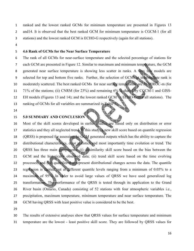
16
ranked and the lowest ranked GCMs for minimum temperature are presented in Figures 13 1
and14. It is observed that the best ranked GCM for minimum temperature is CGCM-1 (for all 2
stations) and the lowest ranked GCM is ECHO-G respectively (again for all stations). 3
4
4.6 Rank of GCMs for the Near Surface Temperature 5
The rank of all GCMs for near-surface temperature and the selected percentage of stations for 6
each GCM are presented in Figure 12. Similar to maximum and minimum temperature, the GCM 7
generated near surface temperature is showing less scatter in ranks. A very few models are 8
selected for top and bottom five ranks. Further, the selection of GCMs at intermediate rank is 9
moderately scattered. The best ranked GCMs for near surface temperature are (i) MIROC-m (for 10
71% of the stations; (ii) CNRM (for 23%) and remaining 6% is shared by CGCM-1 and GISS-11
EH models (Figures 13 and 14); and the lowest ranked GCM is ECHO-G (for all stations). The 12
ranking of GCMs for all variables are summarized in Table 5. 13
14
5.0 SUMMARY AND CONCLUSION 15
Most of the skill scores developed in earlier studies are based only on distribution or error 16
statistics and they all neglected trend. In this study, a new skill score based on quantile regression 17
(QRSS) is proposed for assessing the GCM generated outputs which has the ability to capture the 18
distributional characteristics, error statistics and most importantly time evolution or trend. The 19
QRSS has three main components: (i) dissimilarity skill score based on the bias between the 20
GCM and the historically observed data; (ii) trend skill score based on the time evolving 21
processes; and (iii) quantiles that represent distributional changes across the data. The quantile 22
regression is carried out at different quantile levels ranging from a minimum of 0.05% to a 23
maximum of 95%. In order to avoid large values of QRSS we have used generalized log 24
transformation. The performance of the QRSS is tested through its application to the Grand 25
River basin (Ontario, Canada) consisting of 52 stations with four atmospheric variables i.e., 26
precipitation, maximum temperature, minimum temperature and near surface temperature. The 27
GCM having QRSS with least positive value is considered to be the best. 28
29
The results of extensive analyses show that QRSS values for surface temperature and minimum 30
temperature are the lowest - least positive skill score. They are followed by QRSS values for 31

17
maximum temperature and precipitation. It is observed that for the Grand River basin case study, 1
precipitation has the maximum number of opposite trends in quantile slopes. It is followed by 2
maximum temperature. On the other hand both the near surface temperature and the minimum 3
temperature have perfectly matching trends across all the quantiles. The percentage of stations 4
having same ranks across all the GCMs varies significantly in case of precipitation, whereas the 5
variation is minimal for other three variables. 6
7
In case of precipitation not one model is shown to be the best for all the stations. However, in 8
case of other three variables one GCM is often selected at all the stations. 9
Among all the GCMs considered for the Grand River Basin, the MIROC-m is considered to be 10
the best GCM for near surface temperature and maximum temperature, MRI for precipitation and 11
CGCM-1 for minimum temperature. The ECHO-G is ranked the lowest for near surface 12
temperature, maximum temperature and minimum temperature and CCSM is the lowest ranked 13
GCM for precipitation. 14
15
The main focus of the paper is the introduction of the new skill score using quantile regression. 16
The application of methodology in the presented research is limited to: (i) one river basin; and 17
(ii) CMIP3 datasets. The following issues are not addressed in this paper and are considered for 18
future explorations: 19
1. Instead of ranking the models using QRSS, the GCM scores can be easily converted into 20
weights for creating the ensemble of GCMs. One way of converting the QRSS is to 21
rescale the QRSS between 0 and 1, i.e., make the least QRSS equal to one and maximum 22
QRSS to zero. The following equation ensures that the weights of all members of an 23
ensemble of GCM outputs are in between 0 and 1 24
25
min
max min
1K K
K ii K K
QRSS QRSSW
QRSS QRSS
−= + −
(22) 26
27
where K
iW is the weight of the GCM at ‘ith
’ rank after applying QRSS and K is the station. 28
Note that the above equation converts the low QRSS (best GCM) to highest weight 29
(closer to one) and vice-a-versa. 30

18
2. In this study we have adopted generalized log transformation which has a parameter λ . 1
Any other transformation can be adopted which is independent of parameters and can 2
preserve the trends present in the datasets. 3
3. The parameters of the quantile regression are based on single-site and for uni-variate 4
data. The study is in progress to use multi-site multi-variate quantile regression to capture 5
spatial and temporal characteristics. 6
4. The bootstrap technique used to generate synthetic series is single-site and for uni-variate 7
data. To model strong spatial and inter-variable correlations (that usually exists in hydro-8
climatic data) a multi-site multivariate bootstrap (Li 2013; Srivastav and Simonovic, 9
2014) can be used to generate replicates in order to obtain the parameters of the linear 10
quantile regression. 11
12
The research is also in progress to apply this approach to more stations across Canada and use 13
new climate models from CMIP5. 14
15
ACKNOWLEDGEMENTS 16
The authors would like to acknowledge the financial support by the Canadian Water Network 17
Project under Evolving Opportunities for Knowledge Application Grant to the second author. 18
The authors would like to thank the Program for Climate Model Diagnosis and Intercomparison 19
(PCMDI) for their archives of CMIP3 weather data. We acknowledge Environment Canada for 20
providing the atmospheric observed data used in this research. 21
22
23
24
25
26
27
28
29
30
31

19
REFERENCES 1
2
Bürger G., Murdock TQ, Werner AT, Sobie SR, Cannon AJ (2012) Downscaling Extremes - An 3
Intercomparison of Multiple Statistical Methods for Present Climate. J. Climate. 25: 4
4366–4388. doi: http://dx.doi.org/10.1175/JCLI-D-11-00408.1 5
Dessai S, Lu XF, Hulme M (2005) Limited sensitivity analysis of regional climate change 6
probabilities for the 21st century. Journal of Geophysical Research-Atmospheres, 110. 7
Esfahani AA, Michael JF (2014) Forecasting conditional climate-change using a hybrid 8
approach, Environmental Modelling & Software, Volume 52, Pages 83-97, ISSN 1364-9
8152, http://dx.doi.org/10.1016/j.envsoft.2013.10.009. 10
Franzke C (2013) A novel method to test for significant trends in extreme values in serially 11
dependent time series. Geophysical Research Letters, 40(7), 1391–1395. 12
doi:10.1002/grl.50301 13
Giorgi F, Mearns LO (2002) Calculation of average, uncertainty range, and reliability of regional 14
climate changes from AOGCM simulations via the"Reliability Ensemble Averaging" 15
(REA) method, Journal of Climate 15 (10), pp. 1141-1158. 16
Johnson F, Sharma A (2009) Measurement of GCM Skill in Predicting Variables Relevant for 17
Hydroclimatological Assessments. Journal of Climate, 22(16), 4373–4382. 18
doi:10.1175/2009JCLI2681.1 19
Gaur A, Simonovic SP (2013) Climate Change Impact on Flood Hazard in the Grand River 20
Basin, London, Ontario, Canada. Water Resources Research Report no. 084, Facility for 21
Intelligent Decision Support, Department of Civil and Environmental Engineering, 22
London, Ontario, Canada, 92 pages. ISBN: (print) 978-0-7714-3063-3; (online) 978-0-23
7714-3064-0. 24
Gleckler PJ, Taylor KE, Doutriaux C (2008) Performance metrics for climate models. J. 25
Geophys. Res., 113, D06104, doi:10.1029/2007JD008972 26
Kay AL, Davies HN, Bell VA, Jones RG (2009) Comparison of uncertainty sources for climate 27
change impacts: Flood frequency in England, Climatic Change, 92 (1-2), pp. 41-63. 28
Kendon EJ, Rowell DP, Jones RG, Buonomo E (2008) Robustness of future changes in local 29
precipitation extremes (2008) Journal of Climate, 21 (17), pp. 4280-4297. 30

20
Kim JS, Jain S (2010) High-resolution streamflow trend analysis applicable to annual decision 1
calendars: a western United States case study. Climatic Change, 102(3-4), 699–707. 2
doi:10.1007/s10584-010-9933-3 3
Koenker R (2005) Quantile Regression. Cambridge University Press, New York. Koenker, R., 4
Bassett, G., 1978. Regression quantiles. Econometrica 46 (1), 33–50. 5
Koenker R (2006) quantreg: Quantile Regression. R package version 4.01, http://www.r-6
project.org 7
Koenker R, Hallock KF (2001) Quantile regression. J. Econ. Perspect. 15 (4), 143– 156. 8
Koenker R, Schorfheide F (1994) Quantile spline models for global temperature change. Clim. 9
Change 28 (4), 395–404. 10
Murphy JM, Sexton DMH, Barnett DN, Jones GS, Webb MJ, Collins M (2004) Quantification of 11
modelling uncertainties in a large ensemble of climate change simulations. Nature, 12
430(7001), 768-772. 13
Li Z (2013) A new framework for multi-site weather generator: a two-stage model combining a 14
parametric method with a distribution-free shuffle procedure, Climate Dynamics, 15
DOI:10.1007/s00382-013-1979-2 16
Perkins SE, Pitman AJ, Holbrook NJ, McAneney J (2007) Evaluation of the AR4 climate 17
models’ simulated daily maximum temperature, minimum temperature, and precipitation 18
over Australia using probability density functions. J. Climate. 20, 4356– 4376. 19
Tareghian R, Rasmussen PF (2013) Statistical downscaling of precipitation using quantile 20
regression. Journal of Hydrology, 487, 122–135. doi:10.1016/j.jhydrol.2013.02.029 21
Prudhomme C, Davies H (2009) Assessing uncertainties in cli- mate change impact analyses on 22
the river flow regimes in the UK, Part 2: future climate, Climatic Change, 93(1–2), 197–23
222 24
Suraje D, Hulme M (2007) Assessing the robustness of adaptation decisions to climate change 25
uncertainties: A case study on water resources management in the East of England, 26
Global Environmental Change, Volume 17, Issue 1, Pages 59-72, 27
http://dx.doi.org/10.1016/j.gloenvcha.2006.11.005. 28
Srivastav RK, Simonovic SP (2014) Multi-site, Multivariate Weather Generator using Maximum 29
Entropy Boostrap, Climate Dynamics (in print) 30

21
Teutschbein C, Wetterhall F, Seibert J (2011) Evaluation of different downscaling techniques for 1
hydrological climate-change impact studies at the catchment scale, Climate Dynamics, 2
37(9–10), 2087–2105, doi:10.1007/s00382-010-0979- 8. 3
Wilby RL, Harris I (2006) A framework for assessing uncertainties in climate change impacts: 4
Low flow scenarios for the River Thames, UK. Water Resources Research, 42, W02419, 5
doi:10.1029/2005WR004065 6
Woldemeskel FM, Sharma A, Sivakumar B, Mehrotra R (2012) An error estimation method for 7
precipitation and temperature projections for future climates. Journal of Geophysical 8
Research–Atmospheres, 117, D22104, doi:10.1029/2012JD018062 9
Yokoi S et al (2011) Application of Cluster Analysis to Climate Model Performance Metrics. 10
Journal of Applied Meteorology and Climatology, 50, 1666-1675 11
Zhou L, Rocke DM (2005) An expression index for Affymetrix GeneChips based on the 12
generalized logarithm, Bioinformatics, 21 (21), pp. 3983-3989. 13
14
15
16
17
18
19
20
21
22
23
24
25
26
27
28
29
30
31

22
List of Tables 1
Table 1: List of model performance indices or skill scores proposed in the literature for 2
assessment of the GCM outputs 3
4
Table 2: Basic characteristics of weather stations located in the Grand River basin (Ontario. 5
Canada) 6
7
Table 3: The list of GCM models available with daily data 8
9
Table 4: Name of GCM models including realizations for atmospheric variables - precipitation, 10
maximum temperature, minimum temperature and near surface temperature 11
12
Table 5: The highest and the lowest ranked GCM models with respect to variables and 13
percentage of stations selected. 14
15
List of Figures 16
Figure 1: Hypothetical example of possible trends of quantile regression line for αth
quantile 17
level. Panels (a) and (b) are undesirable representation of time evolution process between the 18
GCM output and the historical observed data and hence the skill scores are penalized; whereas 19
the panels (b) and (c) are desirable representation of datasets and hence the skill scores are not 20
penalized. 21
Figure 2: The Grand River basin showing the location of weather stations 22
Figure 3: Quantile regression lines for various quantile levels selected (0.05, 0.15, 0.25, 0.35, 23
0.5, 0.65, 0.75, 0.85, 0.95) – precipitation. The top panels show results for historical data and the 24
bottom panels show results for GCM data. The left side panels are without transforming the data 25
and the right side panels are after transforming the data using generalized log (GLog) 26
transformation. 27
Figure 4: Quantile regression lines for various quantile levels selected (0.05, 0.15, 0.25, 0.35, 28
0.5, 0.65, 0.75, 0.85, 0.95) – maximum temperature. The top panels show results for historical 29
data and the bottom panels show results for GCM data. The left side panels are without 30
transforming the data and the right side panels are after transforming the data using generalized 31
log (GLog) transformation. 32
Figure 5: Quantile regression lines for various quantile levels selected (0.05, 0.15, 0.25, 0.35, 33
0.5, 0.65, 0.75, 0.85, 0.95) – minimum temperature. The top panels show results for historical 34
data and the bottom panels show results for GCM data. The left side panels are without 35
transforming the data and the right side panels are after transforming the data using generalized 36
log (GLog) transformation. 37
Figure 6: Quantile regression lines for various quantile levels selected (0.05, 0.15, 0.25, 0.35, 38
0.5, 0.65, 0.75, 0.85, 0.95) – near surface temperature. The top panels show results for historical 39
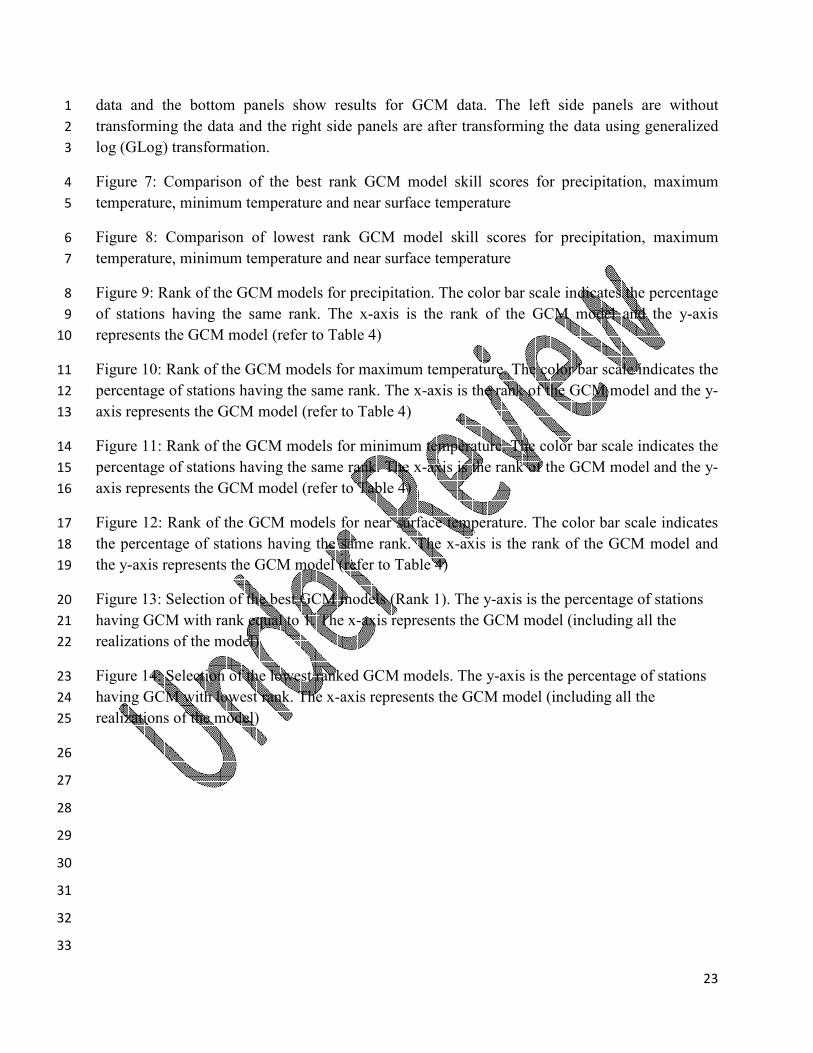
23
data and the bottom panels show results for GCM data. The left side panels are without 1
transforming the data and the right side panels are after transforming the data using generalized 2
log (GLog) transformation. 3
Figure 7: Comparison of the best rank GCM model skill scores for precipitation, maximum 4
temperature, minimum temperature and near surface temperature 5
Figure 8: Comparison of lowest rank GCM model skill scores for precipitation, maximum 6
temperature, minimum temperature and near surface temperature 7
Figure 9: Rank of the GCM models for precipitation. The color bar scale indicates the percentage 8
of stations having the same rank. The x-axis is the rank of the GCM model and the y-axis 9
represents the GCM model (refer to Table 4) 10
Figure 10: Rank of the GCM models for maximum temperature. The color bar scale indicates the 11
percentage of stations having the same rank. The x-axis is the rank of the GCM model and the y-12
axis represents the GCM model (refer to Table 4) 13
Figure 11: Rank of the GCM models for minimum temperature. The color bar scale indicates the 14
percentage of stations having the same rank. The x-axis is the rank of the GCM model and the y-15
axis represents the GCM model (refer to Table 4) 16
Figure 12: Rank of the GCM models for near surface temperature. The color bar scale indicates 17
the percentage of stations having the same rank. The x-axis is the rank of the GCM model and 18
the y-axis represents the GCM model (refer to Table 4) 19
Figure 13: Selection of the best GCM models (Rank 1). The y-axis is the percentage of stations 20
having GCM with rank equal to 1. The x-axis represents the GCM model (including all the 21
realizations of the model) 22
Figure 14: Selection of the lowest ranked GCM models. The y-axis is the percentage of stations 23
having GCM with lowest rank. The x-axis represents the GCM model (including all the 24
realizations of the model) 25
26
27
28
29
30
31
32
33

24
Tables
Table 2: Basic characteristics of weather stations located in the Grand River basin (Ontario. Canada)
S.No Station
Name
Longitude
(degrees)
Latitude
(degrees) Elevation
S.No Station
Name
Longitude
(degrees)
Latitude
(degrees) Elevation
1 Apps Mill -80.383 43.133 230.1 27 Grand Valley WPCP -80.333 43.883 464.8
2 Arthur -80.567 43.817 452 28 Guelph Arboretum -80.217 43.55 327.7
3 Ayr -80.45 43.283 289.6 29 Guelph Oac -80.233 43.517 333.8
4 Blue Acton -80.05 43.6 365.8 30 Guelph Physics Dept -80.267 43.55 340.5
5 Blue Corwhin -80.117 43.533 350.5 31 Guelph Turfgrass CS -80.217 43.55 325
6 Blue Rockwood -80.117 43.583 350.5 32 Haysville -80.633 43.35 320
7 Blue Scout -80.083 43.617 342.9 33 Hillsburgh -80.167 43.767 427
8 Blue Springs Creek -80.117 43.633 373.4 34 Kitchener -80.5 43.433 320
9 Brantford Morell -80.283 43.15 198.1 35 Kitchener City Eng 1 -80.483 43.45 320
10 Burford -80.433 43.1 259.1 36 Kitchener City Eng 2 -80.483 43.45 281.9
11 Cambridge Galt -80.317 43.33 268.2 37 Kitchener OWRC -80.433 43.4 321.6
12 Cambridge-Stewart -80.3 43.35 289 38 Kitchener/ Waterloo -80.379 43.461 342.9
13 Canning -80.45 43.183 259.1 39 Millers Lake -80.383 43.283 304.8
14 Cathcart -80.567 43.117 269.7 40 Monticello -80.4 43.967 481.6
15 Crewsons Corners -80.1 43.617 358.1 41 Morriston -80.117 43.467 304.8
16 Damascus -80.483 43.917 487.7 42 Newton -80.9 43.583 373.4
17 Drumbo -80.55 43.233 304.8 43 Newton -80.883 43.583 382
18 Drumbo Harrington -80.517 43.233 281.9 44 Paris -80.45 43.183 266.7
19 Elmira -80.533 43.6 350.5 45 Preston -80.417 43.4 291.1
20 Elora ACS -80.417 43.65 376.4 46 Preston WPCP -80.35 43.383 272.8
21 Elora RCS -80.417 43.65 376.4 47 Salem -80.47 43.71 430
22 Elora Research Stn -80.417 43.65 376.4 48 Waldemar -80.283 43.883 449.6
23 Falkland -80.45 43.133 262.1 49 Waterloo Fire Hall -80.517 43.467 317
24 Fergus MOE -80.38 43.702 396.2 50 Waterloo WellingtonA -80.383 43.45 317
25 Fergus Shand Dam -80.331 43.735 417.6 51 Waterloo wellington 2 -80.383 43.45 313.6
26 Glen Allan -80.711 43.684 400 52 Waterloo WPCP -80.517 43.483 327.7

25
Table 3: The list of GCM models available with daily data 1
Country Acronym Model
Number of Realizations selected for
each atmospheric variables GCM
Resolution
Group
Name PPT TMAX TMIN
Near Surface
Temperature
Norway BCCR bccr_bccm2_0 1 1 1 1 1.9º x 1.9º Norway
Canada CGCM-1 cccma_cgcm3_1_t47 5 5 5 5 2.8º x 2.8º Canada
Canada CGCM-h cccma_cgcm3_1_t63 1 1 1 1 1.9º x 1.9º
France CNRM cnrm_cm3 1 1 1 1 1.9º x 1.9º France-1
Australia CSIRO3.0 csiro_mk3_0 3 3 3 3 1.9º x 1.9º Australia
Australia CSIRO3.5 csiro_mk3_5 3 3 3 3 1.9º x 1.9º
USA GFDL2.0 gfdl_cm2_0 1 1 1 1 2.0ºx 2.5º USA-1
USA GFDL2.1 gfdl_cm2_1 1 1 1 1 2.0º x 2.5º
USA GISSAOM giss_aom 1 1 1 1 3ºx 4º
USA-2 USA GISS EH giss_model_e_h 1 1 1 1 4º x 5º
USA GISS ER giss_model_e_r 1 1 1 1 4º x 5º
China FGOALS iap_fgoals1_o_g 3 3 3 3 2.8º x 2.8º China
Italy INGV ingv_echam4 1 1 1 1 1.9º x 1.9º Italy
Russia INM inmcm3_0 1 0 0 1 4º x 5º Russia
France IPSL ipsl_cm4 2 2 2 2 2.5° x 3.75° France-2
Japan MIROC-h miroc3_2_hires 0 1 1 0 1.1º x 1.1º Japan-1
Japan MIROC-m miroc3_2_medres 2 2 2 2 2.8º x 2.8º
Germany ECHO-G miub_echo_g 3 3 3 3 3.9ºx 3.9º Germany
Germany ECHAM mpi_echam5 2 2 2 2 1.9º x 1.9º
Japan MRI mri_cgcm2_3_2a 5 5 5 5 2.8º x 2.8º Japan-2
USA CCSM ncar_ccsm3 6 0 0 6 1.4º x 1.4º USA-3
USA PCM ncar_pcm1 3 2 2 3 2.8º x 2.8º
2
3
4
5

26
Table 4: Name of GCM models including realizations for atmospheric variables - precipitation, 1
maximum temperature, minimum temperature and near surface temperature 2
Sl No. GCM
Model Model with Realizations
Sl No. GCM
Model
Model with
Realizations
1 BCCR bccr_bcm2_0_R1 25 IPSL
ipsl_cm4_R1
2
CGCM-1
cccma_cgcm3_1_R1 26 ipsl_cm4_R2
3 cccma_cgcm3_1_R2 27 MIROC-h miroc3_2_hires_R1
4 cccma_cgcm3_1_R3 28 MIROC-m
miroc3_2_medres_R1
5 cccma_cgcm3_1_R4 29 miroc3_2_medres_R2
6 cccma_cgcm3_1_R5 30
ECHO-G
miub_echo_g_R1
7 CGCM-h cccma_cgcm3_1_t63_R1 31 miub_echo_g_R2
8 CNRM cnrm_cm3_R1 32 miub_echo_g_R3
9
CSIRO3.0
csiro_mk3_0_R1 33 ECHAM
mpi_echam5_R1
10 csiro_mk3_0_R2 34 mpi_echam5_R4
11 csiro_mk3_0_R3 35
MRI
mri_cgcm2_3_2a_R1
12
CSIRO3.5
csiro_mk3_5_R1 36 mri_cgcm2_3_2a_R2
13 csiro_mk3_5_R2 37 mri_cgcm2_3_2a_R3
14 csiro_mk3_5_R3 38 mri_cgcm2_3_2a_R4
15 GFDL2.0 gfdl_cm2_0_R1 39 mri_cgcm2_3_2a_R5
16 GFDL2.1 gfdl_cm2_1_R1 40
CCSM
ncar_ccsm3_0_R1
17 GISSAOM giss_aom_R1 41 ncar_ccsm3_0_R3
18 GISS EH giss_model_e_h_R5 42 ncar_ccsm3_0_R5
19 GISS ER giss_model_e_r_R1 43 ncar_ccsm3_0_R6
20
FGOALS
iap_fgoals1_0_g_R1 44 ncar_ccsm3_0_R7
21 iap_fgoals1_0_g_R2 45 ncar_ccsm3_0_R8
22 iap_fgoals1_0_g_R3 46
PCM
ncar_pcm1_R1
23 INGV ingv_echam4_R1 47 ncar_pcm1_R2
24 INM inmcm3_0_R1 48 ncar_pcm1_R4
3
4
Table 5: The highest and the lowest ranked GCM models with respect to variables and 5
percentage of stations selected. 6
7
8
9
10
11
12
13
14
Variable Rank based
on QRSS
GCM Selected (highest percentage of stations
selected)
The highest
ranked
The lowest ranked
Surface
Temperature
1 MIROC-m (72%) ECHO-G (100%)
Minimum
Temperature
1 CGCM-1 (100%) ECHO-G (100%)
Maximum
Temperature
3 MIROC-m (94%) ECHO-G (83%)
Precipitation 4 MRI (65%) CCSM (40%)

27
Figures 1
2
3
4
5
6
7
8
9
10
11
12
13
14
15
16
17
18
19
20
21
22
23
24
25
26
27
28
29
30
31
Figure 1: Hypothetical example of possible trends of quantile regression line for αth
quantile level. Panels (a) and (b) are undesirable representation of time evolution
process between the GCM output and the historical observed data and hence the skill
scores are penalized; whereas the panels (b) and (c) are desirable representation of
datasets and hence the skill scores are not penalized.
0 500 10000
2
4
6
8
10
Time
Vari
able
Opposite Trend Lines
Historical
GCM
(a)
0 500 10000
2
4
6
8
10
Time
Vari
able
Opposite Trend Lines
Historical
GCM
(b)
0 500 10000
2
4
6
8
10
Time
Vari
able
Both Positive Trend Lines
Historical
GCM
(c)
0 500 10000
2
4
6
8
10
Time
Vari
able
Both Negative Trend Lines
Historical
GCM
(d)

28
1
2
3
4
5
6
7
8
9
10
11
12
13
14
15
16
17
18
19
20
21
22
23
24
25
26
27
28
29
30
31
Figure 2: The Grand River basin showing the location of weather stations

29
1
2
3
4
5
6
7
8
9
10
11
12
13
14
15
16
17
18
19
20
21
22
23
24
25
26
27
28
29
30
31
0 5000 10000 15000-2
0
2
4
6
8
10
12
14
16
Time
Pre
cip
ita
tion
GCM Data - Quantile Lines
0.050.05
0.050.050.15 0.15 0.150.25 0.25 0.250.35 0.35 0.35
0.5 0.5 0.5
0.65 0.65 0.65
0.75 0.75 0.75
0.85 0.85 0.85
0.95 0.95 0.95
0 5000 10000 15000-2
0
2
4
6
8
10
12
14
16
Time
Pre
cip
ita
tion
Observed Data - Quantile Lines
0.050.05
0.050.050.15 0.150.15
0.250.25
0.250.35
0.350.35
0.350.5 0.5 0.5 0.50.65 0.65 0.65
0.75 0.75 0.75
0.85 0.85 0.85
0.950.95
0.95
0 5000 10000 150002
2.2
2.4
2.6
2.8
3
3.2
3.4
3.6
3.8
4
Time
Pre
cip
ita
tion
Observed Data - Quantile Lines - GLog Transformation
0.05 0.05 0.050.15 0.15 0.150.25 0.25 0.250.35 0.35 0.350.5 0.5 0.50.65 0.65 0.65
0.75 0.75 0.75
0.85 0.85 0.85
0.95 0.95 0.95
0 5000 10000 150002
2.2
2.4
2.6
2.8
3
3.2
3.4
3.6
3.8
4
Time
Pre
cip
ita
tion
GCM Data - Quantile Lines - GLog Transformation
0.05 0.05 0.050.15 0.15 0.150.25 0.25 0.250.35 0.35 0.350.5 0.5 0.5
0.65 0.65 0.65
0.75 0.75 0.75
0.85 0.85 0.85
0.95 0.95 0.95
Figure 3: Quantile regression lines for various quantile levels selected (0.05, 0.15, 0.25, 0.35, 0.5,
0.65, 0.75, 0.85, 0.95) – precipitation. The top panels show results for historical data and the bottom
panels show results for GCM data. The left side panels are without transforming the data and the
right side panels are after transforming the data using generalized log (GLog) transformation.

30
1
2
3
4
5
6
7
8
9
10
11
12
13
14
15
16
17
18
19
20
21
22
23
24
25
26
27
28
29
30
31
0 5000 10000 15000-15
-10
-5
0
5
10
15
20
25
30
35
Time
TM
AX
GCM Data - Quantile Lines
0.050.05
0.050.05
0.15 0.15 0.15
0.25 0.25 0.25
0.35 0.35 0.35
0.5 0.5 0.5
0.65 0.65 0.65
0.75 0.75 0.75
0.85 0.85 0.85
0.95 0.95 0.95
0 5000 10000 15000-15
-10
-5
0
5
10
15
20
25
30
35
Time
TM
AX
Observed Data - Quantile Lines
0.050.05
0.050.05
0.15 0.15 0.15
0.25 0.25 0.25
0.35 0.35 0.35
0.5 0.5 0.5
0.65 0.65 0.65
0.75 0.75 0.75
0.85 0.85 0.85
0.95 0.95 0.95
0 5000 10000 150000
0.5
1
1.5
2
2.5
3
3.5
4
4.5
5
Time
TM
AX
GCM Data - Quantile Lines - GLog Transformation
0.05 0.05 0.05
0.15 0.15 0.15
0.25 0.25 0.25
0.35 0.35 0.35
0.5 0.5 0.5
0.65 0.65 0.650.75 0.75 0.750.85 0.85 0.850.95 0.95 0.95
0 5000 10000 150000
0.5
1
1.5
2
2.5
3
3.5
4
4.5
5
Time
TM
AX
Observed Data - Quantile Lines - GLog Transformation
0.05 0.05 0.05
0.15 0.15 0.15
0.25 0.25 0.25
0.35 0.35 0.35
0.5 0.5 0.5
0.65 0.65 0.650.75 0.75 0.750.85 0.85 0.850.95 0.95 0.95
Figure 4: Quantile regression lines for various quantile levels selected (0.05, 0.15, 0.25, 0.35, 0.5,
0.65, 0.75, 0.85, 0.95) – maximum temperature. The top panels show results for historical data and
the bottom panels show results for GCM data. The left side panels are without transforming the data
and the right side panels are after transforming the data using generalized log (GLog)
transformation.

31
1
2
3
4
5
6
7
8
9
10
11
12
13
14
15
16
17
18
19
20
21
22
23
24
25
26
27
28
29
30
31
0 5000 10000 15000-30
-25
-20
-15
-10
-5
0
5
10
15
20
25
Time
TM
IN
Observed Data - Quantile Lines
0.050.0
50.05
0.05
0.15 0.15 0.15
0.25 0.25 0.25
0.35 0.35 0.35
0.5 0.5 0.5
0.65 0.65 0.65
0.75 0.75 0.75
0.85 0.85 0.85
0.95 0.95 0.95
0 5000 10000 15000-30
-25
-20
-15
-10
-5
0
5
10
15
20
25
Time
TM
IN
GCM Data - Quantile Lines
0.05
0.05
0.05
0.05
0.15 0.15 0.15
0.25 0.25 0.25
0.35 0.35 0.35
0.5 0.5 0.5
0.65 0.65 0.65
0.75 0.75 0.75
0.85 0.85 0.85
0.95 0.95 0.95
0 5000 10000 150000
0.5
1
1.5
2
2.5
3
3.5
4
4.5
5
Time
TM
IN
Observed Data - Quantile Lines - GLog Transformation
0.05 0.05 0.05
0.15 0.15 0.15
0.25 0.25 0.25
0.35 0.35 0.35
0.5 0.5 0.5
0.65 0.65 0.650.75 0.75 0.750.85 0.85 0.850.95 0.95 0.95
0 5000 10000 150000
0.5
1
1.5
2
2.5
3
3.5
4
4.5
5
Time
TM
INGCM Data - Quantile Lines - GLog Transformation
0.05 0.05 0.05
0.15 0.15 0.15
0.25 0.25 0.25
0.35 0.35 0.35
0.5 0.5 0.5
0.65 0.65 0.650.75 0.75 0.750.85 0.85 0.850.95 0.95 0.95
Figure 5: Quantile regression lines for various quantile levels selected (0.05, 0.15, 0.25, 0.35, 0.5,
0.65, 0.75, 0.85, 0.95) – minimum temperature. The top panels show results for historical data and
the bottom panels show results for GCM data. The left side panels are without transforming the data
and the right side panels are after transforming the data using generalized log (GLog)
transformation.

32
1
2
3
4
5
6
7
8
9
10
11
12
13
14
15
16
17
18
19
20
21
22
23
24
25
26
27
28
29
30
31
0 2000 4000 6000 8000 10000 12000 14000-25
-20
-15
-10
-5
0
5
10
15
20
25
Time
Surf
ace
Tem
pera
ture
GCM Data - Quantile Lines
0.050.0
50.0
50.0
5
0.15 0.15 0.15
0.25 0.25 0.25
0.35 0.35 0.35
0.5 0.5 0.5
0.65 0.65 0.65
0.75 0.75 0.75
0.85 0.85 0.85
0.95 0.95 0.95
0 2000 4000 6000 8000 10000 12000 14000-25
-20
-15
-10
-5
0
5
10
15
20
25
Time
Surf
ace
Tem
pera
ture
Observed Data - Quantile Lines
0.05
0.050.0
50.0
5
0.15 0.15 0.15
0.25 0.25 0.25
0.35 0.35 0.35
0.5 0.5 0.5
0.65 0.65 0.65
0.75 0.75 0.75
0.85 0.85 0.85
0.95 0.95 0.95
0 2000 4000 6000 8000 10000 12000 140000
0.5
1
1.5
2
2.5
3
3.5
4
4.5
5
Time
Surf
ace
Tem
pera
ture
GCM Data - Quantile Lines - GLog Transformation
0.05 0.05 0.05
0.15 0.15 0.15
0.25 0.25 0.25
0.35 0.35 0.35
0.5 0.5 0.5
0.65 0.65 0.650.75 0.75 0.750.85 0.85 0.850.95 0.95 0.95
0 2000 4000 6000 8000 10000 12000 140000
0.5
1
1.5
2
2.5
3
3.5
4
4.5
5
Time
Surf
ace
Tem
pera
ture
Observed Data - Quantile Lines - GLog Transformation
0.05 0.05 0.05
0.15 0.15 0.15
0.25 0.25 0.25
0.35 0.35 0.35
0.5 0.5 0.5
0.65 0.65 0.650.75 0.75 0.750.85 0.85 0.850.95 0.95 0.95
Figure 6: Quantile regression lines for various quantile levels selected (0.05, 0.15, 0.25, 0.35, 0.5,
0.65, 0.75, 0.85, 0.95) – near surface temperature. The top panels show results for historical data and
the bottom panels show results for GCM data. The left side panels are without transforming the data
and the right side panels are after transforming the data using generalized log (GLog)
transformation.

33
1
2
3
4
5
6
7
8
9
10
11
12
13
14
15
16
17
18
19
20
21
22
23
24
25
26
27
28
29
30
31
Figure 7: Comparison of the best rank GCM model skill scores for precipitation,
maximum temperature, minimum temperature and near-surface temperature
Figure 8: Comparison of lowest rank GCM model skill scores for precipitation,
maximum temperature, minimum temperature and near-surface temperature

34
1
2
3
4
5
6
7
8
9
10
11
12
13
14
15
16
17
18
19
20
21
22
23
24
25
26
27
28
29
30
31
Rank
GC
M M
ode
l
Precipitation
10 20 30 40
5
10
15
20
25
30
35
40
45
0
10
20
30
40
50
60
70
80
90
100
Figure 9: Rank of the GCM models for precipitation. The color bar scale indicates the percentage of
stations having the same rank. The x-axis is the rank of the GCM model and the y-axis represents the
GCM model (refer to Table 4)
Rank
GC
M M
ode
l
TMAX
5 10 15 20 25 30 35 40
5
10
15
20
25
30
35
40 0
10
20
30
40
50
60
70
80
90
100
Figure 10: Rank of the GCM models for maximum temperature. The color bar scale indicates the
percentage of stations having the same rank. The x-axis is the rank of the GCM model and the y-axis
represents the GCM model (refer to Table 4)

35
1
2
3
4
5
6
7
8
9
10
11
12
13
14
15
16
17
18
19
20
21
22
23
24
25
26
27
28
29
30
31
Rank
GC
M M
ode
l
TMIN
5 10 15 20 25 30 35 40
5
10
15
20
25
30
35
40 0
10
20
30
40
50
60
70
80
90
100
Figure 11: Rank of the GCM models for minimum temperature. The color bar scale indicates the
percentage of stations having the same rank. The x-axis is the rank of the GCM model and the y-axis
represents the GCM model (refer to Table 4)
Rank
GC
M M
ode
l
Surface Temperature
10 20 30 40
5
10
15
20
25
30
35
40
45
0
10
20
30
40
50
60
70
80
90
100
Figure 12: Rank of the GCM models for near surface temperature. The color bar scale indicates the
percentage of stations having the same rank. The x-axis is the rank of the GCM model and the y-axis
represents the GCM model (refer to Table 4)

36
1
2
3
4
5
6
7
8
9
10
11
12
13
14
15
16
17
18
19
20
21
22
23
24
25
26
27
28
29
30
31
Figure 13: Selection of the best GCM models (Rank 1). The y-axis is the percentage of stations
having GCM with rank equal to 1. The x-axis represents the GCM model (including all the
realizations of the model)
Figure 14: Selection of the lowest ranked GCM models. The y-axis is the percentage of stations
having GCM with lowest rank. The x-axis represents the GCM model (including all the
realizations of the model)

46
Appendix – F: Journal paper on equidistance quantile matching method for updating IDF
curves under climate change
Article Link: http://link.springer.com/article/10.1007%2Fs11269-014-0626-y

47
Appendix – G: List of Previous Reports in the Series
ISSN: (Print) 1913-3200; (online) 1913-3219
In addition to 53 previous reports (No. 01 – No. 53) prior to 2007
Predrag Prodanovic and Slobodan P. Simonovic (2007). Dynamic Feedback Coupling of
Continuous Hydrologic and Socio-Economic Model Components of the Upper Thames River
Basin. Water Resources Research Report no. 054, Facility for Intelligent Decision Support,
Department of Civil and Environmental Engineering, London, Ontario, Canada, 437 pages.
ISBN: (print) 978-0-7714-2638-4; (online) 978-0-7714-2639-1.
Subhankar Karmakar and Slobodan P. Simonovic (2007). Flood frequency analysis using copula
with mixed marginal distributions. Water Resources Research Report no. 055, Facility for
Intelligent Decision Support, Department of Civil and Environmental Engineering, London,
Ontario, Canada, 144 pages. ISBN: (print) 978-0-7714-2658-2; (online) 978-0-7714-2659-9.
Jordan Black, Subhankar Karmakar and Slobodan P. Simonovic (2007). A web-based flood
information system. Water Resources Research Report no. 056, Facility for Intelligent Decision
Support, Department of Civil and Environmental Engineering, London, Ontario, Canada, 133
pages. ISBN: (print) 978-0-7714-2660-5; (online) 978-0-7714-2661-2.
Angela Peck, Subhankar Karmakar and Slobodan P. Simonovic (2007). Physical, economical,
infrastructural and social flood risk - vulnerability analyses in GIS. Water Resources Research
Report no. 057, Facility for Intelligent Decision Support, Department of Civil and Environmental
Engineering, London, Ontario, Canada, 79 pages. ISBN: (print) 978-0-7714-2662-9; (online)
978-0-7714-2663-6.
Predrag Prodanovic and Slobodan P. Simonovic (2007). Development of rainfall intensity
duration frequency curves for the City of London under the changing climate. Water Resources
Research Report no. 058, Facility for Intelligent Decision Support, Department of Civil and
Environmental Engineering, London, Ontario, Canada, 51 pages. ISBN: (print) 978-0-7714-
2667-4; (online) 978-0-7714-2668-1.
Evan G. R. Davies and Slobodan P. Simonovic (2008). An integrated system dynamics model for
analyzing behaviour of the social-economic-climatic system: Model description and model use
guide. Water Resources Research Report no. 059, Facility for Intelligent Decision Support,
Department of Civil and Environmental Engineering, London, Ontario, Canada, 233 pages.
ISBN: (print) 978-0-7714-2679-7; (online) 978-0-7714-2680-3.
Vasan Arunachalam (2008). Optimization Using Differential Evolution. Water Resources
Research Report no. 060, Facility for Intelligent Decision Support, Department of Civil and

48
Environmental Engineering, London, Ontario, Canada, 38 pages. ISBN: (print) 978-0-7714-
2689-6; (online) 978-0-7714-2690-2.
Rajesh R. Shrestha and Slobodan P. Simonovic (2009). A Fuzzy Set Theory Based Methodology
for Analysis of Uncertainties in Stage-Discharge Measurements and Rating Curve. Water
Resources Research Report no. 061, Facility for Intelligent Decision Support, Department of
Civil and Environmental Engineering, London, Ontario, Canada, 104 pages. ISBN: (print) 978-0-
7714-2707-7; (online) 978-0-7714-2708-4.
Hyung-Il Eum, Vasan Arunachalam and Slobodan P. Simonovic (2009). Integrated Reservoir
Management System for Adaptation to Climate Change Impacts in the Upper Thames River
Basin. Water Resources Research Report no. 062, Facility for Intelligent Decision Support,
Department of Civil and Environmental Engineering, London, Ontario, Canada, 81 pages. ISBN:
(print) 978-0-7714-2710-7; (online) 978-0-7714-2711-4.
Evan G. R. Davies and Slobodan P. Simonovic (2009). Energy Sector for the Integrated System
Dynamics Model for Analyzing Behaviour of the Social-Economic-Climatic Model. Water
Resources Research Report no. 063, Facility for Intelligent Decision Support, Department of
Civil and Environmental Engineering, London, Ontario, Canada, 191 pages. ISBN: (print) 978-0-
7714-2712-1; (online) 978-0-7714-2713-8.
Leanna King, Tarana Solaiman and Slobodan P. Simonovic (2009). Assessment of Climatic
Vulnerability in the Upper Thames River Basin. Water Resources Research Report no. 064,
Facility for Intelligent Decision Support, Department of Civil and Environmental Engineering,
London, Ontario, Canada, 62 pages. ISBN: (print) 978-0-7714-2816-6; (online) 978-0-7714-
2817-3.
Slobodan P. Simonovic and Angela Peck (2009). Updated rainfall intensity duration frequency
curves for the City of London under the changing climate. Water Resources Research Report no.
065, Facility for Intelligent Decision Support, Department of Civil and Environmental
Engineering, London, Ontario, Canada, 64 pages. ISBN: (print) 978-0-7714-2819-7; (online)
978-0-7714-2820-3.
Leanna King, Tarana Solaiman and Slobodan P. Simonovic (2010). Assessment of Climatic
Vulnerability in the Upper Thames River Basin: Part 2. Water Resources Research Report no.
066, Facility for Intelligent Decision Support, Department of Civil and Environmental
Engineering, London, Ontario, Canada, 72 pages. ISBN: (print) 978-0-7714-2834-0; (online)
978-0-7714-2835-7.

49
Christopher J. Popovich, Slobodan P. Simonovic and Gordon A. McBean (2010). Use of an
Integrated System Dynamics Model for Analyzing Behaviour of the Social-Economic-Climatic
System in Policy Development. Water Resources Research Report no. 067, Facility for
Intelligent Decision Support, Department of Civil and Environmental Engineering, London,
Ontario, Canada, 37 pages. ISBN: (print) 978-0-7714-2838-8; (online) 978-0-7714-2839-5.
Hyung-Il Eum and Slobodan P. Simonovic (2009). City of London: Vulnerability of
Infrastructure to Climate Change, Background Report #1 - Climate and Hydrologic Modeling.
Water Resources Research Report no. 068, Facility for Intelligent Decision Support, Department
of Civil and Environmental Engineering, London, Ontario, Canada, 103 pages. ISBN: (print)
978-0-7714-2844-9; (online) 978-0-7714-2845-6.
Dragan Sredojevic and Slobodan P. Simonovic (2009). City of London: Vulnerability of
Infrastructure to Climate Change, Background Report #2 - Hydraulic Modeling and Floodplain
Mapping. Water Resources Research Report no. 069, Facility for Intelligent Decision Support,
Department of Civil and Environmental Engineering, London, Ontario, Canada, 147 pages.
ISBN: (print) 978-0-7714-2846-3; (online) 978-0-7714-2847-0.
Tarana A. Solaiman and Slobodan P. Simonovic (2011). Quantifying Uncertainties in the
Modelled Estimates of Extreme Precipitation Events at Upper Thames River Basin. Water
Resources Research Report no. 070, Facility for Intelligent Decision Support, Department of
Civil and Environmental Engineering, London, Ontario, Canada, 167 pages. ISBN: (print) 978-0-
7714-2878-4; (online) 978-0-7714-2880-7.
Tarana A. Solaiman and Slobodan P. Simonovic (2011). Assessment of Global and Regional
Reanalyses Data for Hydro-Climatic Impact Studies in the Upper Thames River Basin. Water
Resources Research Report no. 071, Facility for Intelligent Decision Support, Department of
Civil and Environmental Engineering, London, Ontario, Canada, 74 pages. ISBN: (print) 978-0-
7714-2892-0; (online) 978-0-7714-2899-9.
Tarana A. Solaiman and Slobodan P. Simonovic (2011). Development of Probability Based
Intensity-Duration-Frequency Curves under Climate Change. Water Resources Research Report
no. 072, Facility for Intelligent Decision Support, Department of Civil and Environmental
Engineering, London, Ontario, Canada, 89 pages. ISBN: (print) 978-0-7714-2893-7; (online)
978-0-7714-2900-2.
Dejan Vucetic and Slobodan P. Simonovic (2011). Water Resources Decision Making Under
Uncertainty. Water Resources Research Report no. 073, Facility for Intelligent Decision Support,
Department of Civil and Environmental Engineering, London, Ontario, Canada, 143 pages.
ISBN: (print) 978-0-7714-2894-4; (online) 978-0-7714-2901-9.

50
Angela Peck, Elisabeth Bowering, and Slobodan P. Simonovic (2011). City of London:
Vulnerability of Infrastructure to Climate Change, Final Report. Water Resources Research
Report no. 074, Facility for Intelligent Decision Support, Department of Civil and Environmental
Engineering, London, Ontario, Canada, 66 pages. ISBN: (print) 978-0-7714-2895-1; (online)
978-0-7714-2902-6.
M. Khaled Akhtar, Slobodan P. Simonovic, Jacob Wibe, Jim MacGee and Jim Davies (2011).
An Integrated System Dynamics Model for Analyzing Behaviour of the Social-Energy-
Economy-Climate System: Model Description. Water Resources Research Report no. 075,
Facility for Intelligent Decision Support, Department of Civil and Environmental Engineering,
London, Ontario, Canada, 211 pages. ISBN: (print) 978-0-7714-2896-8; (online) 978-0-7714-
2903-3.
M. Khaled Akhtar, Slobodan P. Simonovic, Jacob Wibe, Jim MacGee and Jim Davies (2011).
An Integrated System Dynamics Model for Analyzing Behaviour of the Social-Energy-
Economy-Climate System: User's Manual. Water Resources Research Report no. 076, Facility
for Intelligent Decision Support, Department of Civil and Environmental Engineering, London,
Ontario, Canada, 161 pages. ISBN: (print) 978-0-7714-2897-5; (online) 978-0-7714-2904-0.
Nick Millington, Samiran Das and Slobodan P. Simonovic (2011). The Comparison of GEV,
Log-Pearson Type 3 and Gumbel Distributions in the Upper Thames River Watershed under
Global Climate Models. Water Resources Research Report no. 077, Facility for Intelligent
Decision Support, Department of Civil and Environmental Engineering, London, Ontario,
Canada, 53 pages. ISBN: (print) 978-0-7714-2898-2; (online) 978-0-7714-2905-7.
Andre Schardong and Slobodan P. Simonovic (2011). Multi-objective Evolutionary Algorithms
for Water Resources Management. Water Resources Research Report no. 078, Facility for
Intelligent Decision Support, Department of Civil and Environmental Engineering, London,
Ontario, Canada, 167 pages. ISBN: (print) 978-0-7714-2907-1; (online) 978-0-7714-2908-8.
Samiran Das and Slobodan P. Simonovic (2012). Assessment of Uncertainty in Flood Flows
under Climate Change. Water Resources Research Report no. 079, Facility for Intelligent
Decision Support, Department of Civil and Environmental Engineering, London, Ontario,
Canada, 67 pages. ISBN: (print) 978-0-7714-2960-6; (online) 978-0-7714-2961-3.
Rubaiya Sarwar, Sarah E. Irwin, Leanna King and Slobodan P. Simonovic (2012). Assessment of
Climatic Vulnerability in the Upper Thames River basin: Downscaling with SDSM. Water
Resources Research Report no. 080, Facility for Intelligent Decision Support, Department of
Civil and Environmental Engineering, London, Ontario, Canada, 65 pages. ISBN: (print) 978-0-
7714-2962-0; (online) 978-0-7714-2963-7.

51
Sarah E. Irwin, Rubaiya Sarwar, Leanna King and Slobodan P. Simonovic (2012). Assessment of
Climatic Vulnerability in the Upper Thames River basin: Downscaling with LARS-WG. Water
Resources Research Report no. 081, Facility for Intelligent Decision Support, Department of
Civil and Environmental Engineering, London, Ontario, Canada, 80 pages. ISBN: (print) 978-0-
7714-2964-4; (online) 978-0-7714-2965-1.
Samiran Das and Slobodan P. Simonovic (2012). Guidelines for Flood Frequency Estimation
under Climate Change. Water Resources Research Report no. 082, Facility for Intelligent
Decision Support, Department of Civil and Environmental Engineering, London, Ontario,
Canada, 44 pages. ISBN: (print) 978-0-7714-2973-6; (online) 978-0-7714-2974-3.
Angela Peck and Slobodan P. Simonovic (2013). Coastal Cities at Risk (CCaR): Generic System
Dynamics Simulation Models for Use with City Resilience Simulator. Water Resources Research
Report no. 083, Facility for Intelligent Decision Support, Department of Civil and Environmental
Engineering, London, Ontario, Canada, 55 pages. ISBN: (print) 978-0-7714-3024-4; (online)
978-0-7714-3025-1.
Abhishek Gaur and Slobodan P. Simonovic (2013). Climate Change Impact on Flood Hazard in
the Grand River Basin, Ontario, Canada. Water Resources Research Report no. 084, Facility for
Intelligent Decision Support, Department of Civil and Environmental Engineering, London,
Ontario, Canada, 92 pages. ISBN: (print) 978-0-7714-3063-3; (online) 978-0-7714-3064-0.
Roshan Srivastav and Slobodan P. Simonovic (2014). Generic Framework for Computation of
Spatial Dynamic Resilience. Water Resources Research Report no. 085, Facility for Intelligent
Decision Support, Department of Civil and Environmental Engineering, London, Ontario,
Canada, 81 pages. ISBN: (print) 978-0-7714-3067-1; (online) 978-0-7714-3068-8.
Angela Peck and Slobodan P. Simonovic (2014). Coupling System Dynamics with Geographic
Information Systems: CCaR Project Report. Water Resources Research Report no. 086, Facility
for Intelligent Decision Support, Department of Civil and Environmental Engineering, London,
Ontario, Canada, 60 pages. ISBN: (print) 978-0-7714-3069-5; (online) 978-0-7714-3070-1.
Sarah Irwin, Roshan Srivastav and Slobodan P. Simonovic (2014). Instruction for Watershed
Delineation in an ArcGIS Environment for Regionalization Studies. Water Resources Research
Report no. 087, Facility for Intelligent Decision Support, Department of Civil and Environmental
Engineering, London, Ontario, Canada, 45 pages. ISBN: (print) 978-0-7714-3071-8; (online)
978-0-7714-3072-5.