water resources of lexington county, south …
TRANSCRIPT
WATER RESOURCESOF LEXINGTON COUNTY,
SOUTH CAROLINA
STATE OF SOUTH CAROLINADEPARTMENT OF NATURAL
RESOURCES
LAND, WATER AND CONSERVATION DIVISION
WATER RESOURCESREPORT 38
2006
WATER RESOURCESOF
LEXINGTON COUNTY, SOUTH CAROLINA
byKaren W. Agerton
and Samuel E. Baker
STATE OF SOUTH CAROLINADEPARTMENT OF NATURAL RESOURCES
Land, Water and Conservation DivisionWater Resources Report 38
2006
STATE OF SOUTH CAROLINA
The Honorable Mark Sanford, Governor
South Carolina Department of Natural Resources
Board Members
Michael G. McShane, Chairman . . . . . . . . . . . . . . . . . . . . . . . . . . . . . . . . . . . . . . . . . . . . . . . . .Member-at-Large
R. Michael Campbell, II, Vice-Chairman . . . . . . . . . . . . . . . . . . . . . . . . . . . . . . . . . . 2nd Congressional District
Vacant . . . . . . . . . . . . . . . . . . . . . . . . . . . . . . . . . . . . . . . . . . . . . . . . . . . . . . . . . . . . . . 1st Congressional District
Stephen L. Davis . . . . . . . . . . . . . . . . . . . . . . . . . . . . . . . . . . . . . . . . . . . . . . . . . . . . . .3rd Congressional District
Vacant . . . . . . . . . . . . . . . . . . . . . . . . . . . . . . . . . . . . . . . . . . . . . . . . . . . . . . . . . . . . . . 4th Congressional District
Frank Murray, Jr. . . . . . . . . . . . . . . . . . . . . . . . . . . . . . . . . . . . . . . . . . . . . . . . . . . . . . . 5th Congressional District
John P. Evans. . . . . . . . . . . . . . . . . . . . . . . . . . . . . . . . . . . . . . . . . . . . . . . . . . . . . . . . . 6th Congressional District
John E. Frampton, Director
Land, Water and Conservation Division
Alfred H. Vang, Deputy Director
A.W. Badr, Ph.D., Chief, Hydrology Section
II

CONTENTS
PageAbstract
Introduction Physiography and surface drainage ............................................................................................................... 1 Climate .......................................................................................................................................................... 2 Population and economics ............................................................................................................................. 5 Well-numbering system ................................................................................................................................. 5
Geology .................................................................................................................................................................. 7
Water use .............................................................................................................................................................. 10
Ground-water resources ....................................................................................................................................... 10 Water levels ................................................................................................................................................ 11
Aquifer properties ....................................................................................................................................... 14 Transmissivity ...................................................................................................................................... 16 Hydraulic conductivity ......................................................................................................................... 16 Storage coefficient ............................................................................................................................... 16
Well hydraulics ............................................................................................................................................ 16 Well yields............................................................................................................................................ 17 Specific capacity .................................................................................................................................. 17 Well efficiency ..................................................................................................................................... 17
Wells ............................................................................................................................................................ 17 Public-supply wells .............................................................................................................................. 17 Irrigation and industrial wells .............................................................................................................. 17 Domestic wells ..................................................................................................................................... 17
Ground-water quality .................................................................................................................................. 18 Sand wells ............................................................................................................................................ 18 Rock wells ............................................................................................................................................ 20 Radionuclides ....................................................................................................................................... 20
Surface-water resources ....................................................................................................................................... 22 Rivers of Lexington County ........................................................................................................................ 22 Saluda River ......................................................................................................................................... 24 Congaree River .................................................................................................................................... 25 North Fork Edisto River ...................................................................................................................... 27
Lake Murray ................................................................................................................................................ 29
Other lakes and ponds ................................................................................................................................. 31
Summary ............................................................................................................................................................. 31
References ............................................................................................................................................................ 33
III

FIGURES
Page
1. Physiographic provinces and drainage basins of Lexington County, S.C. ................................................... 2
2. Lexington County land cover ....................................................................................................................... 3
3. Lexington County average monthly temperatures, 1949-2002 .................................................................... 4
4. Lexington County average precipitation by month, 1949-2002 ................................................................... 4
5. Average precipitation by year, 1949-2002, in Lexington County ................................................................ 5
6. Illustration of DNR well-grid system ........................................................................................................... 6
7. Generalized geology of Lexington County, modified from Maybin and Nystrom (1995) .......................... 7
8. Peachtree Rock Preserve, Lexington County, S.C. ..................................................................................... 8
9. Approximate contours on the bedrock surface in Lexington County ......................................................... 9
10. Generalized subsurface geology of Lexington County, modified from Aucott and others, (1987) ............ 9
11. Well description and hydrograph for well LEX-79 .................................................................................... 11
12. Well description and hydrograph for well LEX-88 .................................................................................... 12
13. Well description and hydrograph for well LEX-844 .................................................................................. 13
14. Location of wells from which pumping tests were used in this study ....................................................... 14
15. Typical well construction of rock and sand wells in Lexington County, modified from Mitchell, (1995) 17
16. Location of wells for which chemical analyses appear in Table 8 for Lexington County ......................... 20
17. Annual mean streamflow for the period of record for the Saluda, Congaree and North Fork Edisto Rivers .............................................................................................................................................. 22
18. Monthly mean streamflow for the Saluda, Congaree, and North Fork Edisto Rivers ................................ 22
19. Location of USGS stream-flow gaging stations on the lower Saluda, Congaree, and North Fork Edisto Rivers............................................................................................................................ 23
20. Flow-duration curve for the lower Saluda River near Columbia (1925-2001) .......................................... 24
21. Flow-duration curve for Congaree River at Columbia (1940-2001) .......................................................... 26
22. Annual mean streamflow for Congaree Creek in Lexington County, S.C. ................................................ 27
23. Monthly mean streamflow for Congaree Creek in Lexington County, S.C. .............................................. 27
24. Flow-duration curve for the North Fork Edisto River at Orangeburg (1939-2000) ................................... 28
25. Hydrograph of Lake Murray showing lake levels, 1996-2002 ................................................................... 30
IV

TABLESPage
1. Average daily water use in Lexington County, 2001, in mgd ..................................................................... 10
2. Average daily water use for public and rural domestic supply in Lexington County, 2003, in mgd .................................................................................................................................. 10
3. Pumping test data for wells in Lexington County, S.C. .............................................................................. 15
4. Comparison of transmissivity values (gpd/ft) for 20 sand wells in Lexington County ............................... 16
5. Comparison of hydraulic-conductivity values for aquifer tests in the Coastal Plain of Lexington County ................................................................................................................................... 16
6. Static water levels and yields from more than 500 sand wells drilled in Lexington County in 2001 ........................................................................................................................... 18
7. Static water levels and yields for 231 rock wells drilled in Lexington County in 2001 ............................. 18
8. Chemical analyses of water from selected sand and rock wells in Lexington County ............................... 19
9. Range of hardness, adapted from Durfor and Becker, (1964) ..................................................................... 20
10. Maximum contaminent levels for radionuclides (EPA 816-F-02-013 July 2002) ...................................... 21
11. Flow statistics for USGS stream-gage stations in and around Lexington County ...................................... 23
V


�
WATER RESOURCES OF LEXINGTON COUNTY, SOUTH CAROLINA
by
Karen W. Agerton and Samuel E. Baker
ABSTRACT Lexington County encompasses an area of 700 square miles in west-central South Carolina. The Fall Line traverses the county, placing the northern third in the Piedmont and the rest in the Coastal Plain. This has produced two vastly different aquifer systems; hard crystalline rocks and unconsolidated sand.
Water use in Lexington County is about equally divided between surface water and ground water. In 2003, 12 mgd (million gallons per day) were obtained from Lake Murray and the Saluda River, and about 11 mgd were obtained from wells, much of the latter for rural domestic use. The largest public-supply water system in the county is the city of West Columbia, which obtains its water from Lake Murray and the Saluda River.
Wells in the Piedmont rocks rarely produce more than 10 gpm (gallons per minute), and dry holes are common, forcing larger water users to rely on surface water. Sand aquifers have not been heavily tapped and are capable of yielding up to 2000 gpm to wells in the southern part of the county. Pumping tests indicate transmissivities ranging from 1,500 to 55,000 gpd/ft (gallons per day per foot), and specific capacities of sand wells can be more than 25 gpm.
Ground-water quality for rock wells in the Piedmont and sand wells in the Coastal Plain is generally good and the latter often resembles that of rainwater. Excessive levels of radionuclides (226Ra and 228Ra), however, have been reported in some wells in the county since the mid-1970’s. Several sand and rock wells have produced water containing excessive iron and manganese; no other constituents exceed the maximum contaminant levels established by the U.S. Environmental Protection Agency’s National Drinking Water Standards. The sand wells typically have low (acidic) pH values.
Of the three major rivers that drain the county, the Congaree River has the largest annual mean flow, 8,946 cfs (cubic feet per second); it is formed by the confluence of the Saluda and Broad Rivers. The lower Saluda is regulated, according to power demand, by releases from Lake Murray at the Saluda Dam and has the second-highest annual mean flow (2,794 cfs). Draining the western section of the county, the North Fork Edisto River has an annual mean flow of 766 cfs. Lake Murray, the fifth-largest lake in the State, is located in the northern part of the county and contains more than 2 million acre-feet of water.
Surface-water quality is fair, with over 65 percent of the State-monitored water-quality stations meeting the guidelines for several types of uses; however, when water quality standards are not met, it has been predominately due to pH and fecal-coliform bacteria infractions.
INTRODUCTION Lexington County was first named Saxe Gotha Township, around 1733. Settlement began when the British established a trading post on the Congaree River about 1718. The settlement eventually became the town of Granby (present-day Cayce) and was the county seat until 1818, when it was moved to Lexington where it remains today.
In 1930 the Saluda Dam was completed for power generation, and Lake Murray was formed. The Saluda Dam was the world’s largest earthen dam until the Aswan High Dam was completed in 1970 in Egypt. Today Lake Murray is the fifth largest lake in the State and provides exceptional recreational opportunities. Additionally, it is also used for power production by the Saluda Hydro Plant and for cooling purposes at the McMeekin Station which is a coal-firing plant located just below the dam.
Congaree Creek Heritage Preserve and Shealy’s Pond Heritage Preserve, both located in Lexington County, are two of the 51 Heritage Preserve sites in South Carolina. The South Carolina Department of Natural Resources (DNR) Heritage Trust Program was created in 1976 to preserve and
protect endangered species and natural and cultural lands. Congaree Creek Heritage Preserve consists of 627 acres that border the Congaree River and the city of Cayce and contains the site of the Saxe Gotha Township and town of Granby. Shealy’s Pond Heritage Preserve encompasses 62 acres along Scouter Creek about 13 miles southwest of Columbia. It was established to protect the mature Atlantic white cedar forest, along with several rare-plant species.
PHYSIOGRAPHY AND SURFACE DRAINAGE
Local topography is characterized by rolling hills with elevations commonly ranging from 250 ft (feet) above sea level along the major rivers to nearly 750 ft in the northeastern part of the county. The Fall Line, a geologic boundary that divides the State – and Lexington County – into two physiographic provinces, runs generally parallel to U.S. Highway 1 in a northeasterly direction (Fig. 1 ). The Piedmont province, which is northwest of the Fall Line and occupies the upper third of the county, consists of hard, crystalline rocks. The lower two-thirds of the county is in the Coastal Plain province and consists of unconsolidated sand and clay formations.
2
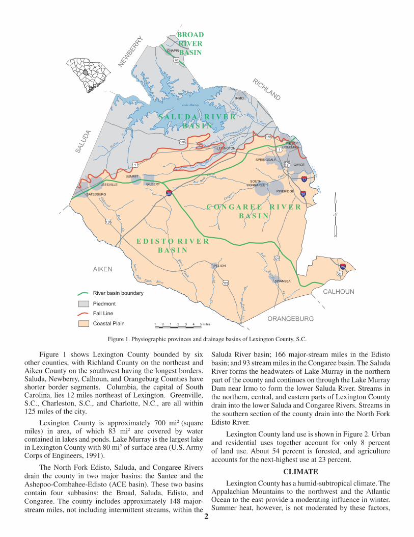
Figure 1 shows Lexington County bounded by six other counties, with Richland County on the northeast and Aiken County on the southwest having the longest borders. Saluda, Newberry, Calhoun, and Orangeburg Counties have shorter border segments. Columbia, the capital of South Carolina, lies 12 miles northeast of Lexington. Greenville, S.C., Charleston, S.C., and Charlotte, N.C., are all within 125 miles of the city.
Lexington County is approximately 700 mi2 (square miles) in area, of which 83 mi2 are covered by water contained in lakes and ponds. Lake Murray is the largest lake in Lexington County with 80 mi2 of surface area (U.S. Army Corps of Engineers, 1991).
The North Fork Edisto, Saluda, and Congaree Rivers drain the county in two major basins: the Santee and the Ashepoo-Combahee-Edisto (ACE basin). These two basins contain four subbasins: the Broad, Saluda, Edisto, and Congaree. The county includes approximately 148 major-stream miles, not including intermittent streams, within the
Figure 1. Physiographic provinces and drainage basins of Lexington County, S.C.
Saluda River basin; 166 major-stream miles in the Edisto basin; and 93 stream miles in the Congaree basin. The Saluda River forms the headwaters of Lake Murray in the northern part of the county and continues on through the Lake Murray Dam near Irmo to form the lower Saluda River. Streams in the northern, central, and eastern parts of Lexington County drain into the lower Saluda and Congaree Rivers. Streams in the southern section of the county drain into the North Fork Edisto River.
Lexington County land use is shown in Figure 2. Urban and residential uses together account for only 8 percent of land use. About 54 percent is forested, and agriculture accounts for the next-highest use at 23 percent.
CLIMATE
Lexington County has a humid-subtropical climate. The Appalachian Mountains to the northwest and the Atlantic Ocean to the east provide a moderating influence in winter. Summer heat, however, is not moderated by these factors,

3
Figure 2. Lexington County land cover.
and Lexington County is often the hottest part of the State. Figure 3 illustrates the temperature pattern throughout the year. The average growing season in Lexington County is about 218 days. Typically, the last spring freeze occurs in late March and the first fall freeze in early November. The annual average temperature is 63.1°F (Fahrenheit). Lexington County essentially has three seasons: spring, summer, and fall. Winter is an alternating pattern of late-fall and early-spring days.
Spring weather is variable, with cold days alternating with mild. Thunderstorms are common in spring, but most are not severe. Tornadoes and hailstorms can occur but are not frequent. Since 1950, several tornadoes have touched down in Lexington County; the most destructive were in 1972, 1974, 1989, and 1994. The 1994 tornado hit the town of Lexington at about noon on August 16, injured 40 people, and did approximately 50 million dollars in damage.
The summer season in Lexington County is long, extending from May to September. Few cold fronts reach
Lexington County during the summer months, owing to the blocking influence of the Bermuda High (a semipermanent, subtropical area of high pressure in the North Atlantic Ocean that migrates east and west with varying central pressure). As a result, the summer heat persists, with temperatures in the 90’s being common. On average, there are about 6 days with temperatures above 100°F (Fahrenheit) during summer. The average maximum temperature in July is 92°F. The highest official temperature recorded in Lexington County is 107°F. This temperature was reached at Pelion on July 13, 1980, and at the Columbia Airport on June 27, 1954, and again on August 21, 1983. A southwesterly airflow around the west side of the Bermuda high brings moisture into the State, resulting in many thunderstorms during June, July, and August. July is usually the wettest month, with an average of 5.12 inches of rain. The highest official 1-day rainfall in Lexington County was 7.10 inches at Pelion on September 4, 1998. A typical year may see one or more tropical systems impact the county in late summer and early fall.

�
Figure 3. Lexington County average monthly temperatures, 1949-2002.
Figure 4. Lexington County average precipitation by month, 1949-2002.
Fall is the driest season in Lexington County. The average rainfall for November is 2.66 inches. There are many days in October and November with a high temperature in the 70’s and clear, blue skies. Cooler weather usually starts in late November, lasts through mid-March, and consists of modified polar air masses that push through the State. Snowfall events and winter storms rarely occur more than three times a year in Lexington County. The average minimum daily temperature in January is 33°F.
Winters are mild in Lexington County and consist of warm and cold days, with the average temperature in the mid 40’s. A typical winter day could see clear skies with a high temperature in the 70’s or rain and temperatures in the 30’s. Snowstorms and ice storms are rare. Lexington County has a 30- to 40- percent chance of a snow event in any year. The largest storm, on February 9-10, 1973, resulted in more than
16 inches of snow. Snow amounts of 1 to 2 inches are more common, with the earliest recorded on November 9, 1913, and the latest on April 3, 1915. A winter storm on January 2-3, 2002, left 5 to 6 inches of snow and ice in Lexington County. Other significant ice storms occurred in January of 1973 and January of 2004. Loss of electric power is usually the worst effect of these storms.
Precipitation is variable throughout the year, with midsummer normally being the wettest period and fall the driest (Fig. 4).
Normally, wet and dry years seem to alternate; however, some periods of several dry years occur. Droughts have occurred in 1954-55, 1986, 1996, and 1998-2002. The historical average annual precipitation for Lexington County is shown in Figure 5. The annual average precipitation is 47.56 inches.

�
Figure 5. Average precipitation by year, 1949-2002, in Lexington County.
The period from 1998 through 2002 was the worst drought on record for South Carolina and was classified as an extreme drought. The lack of normal rainfall for four consecutive years severely stressed the State’s water resources. The water table dropped 10 ft in many locations, and even the deeper aquifers declined to record low levels. Over 65 percent of the State’s streams reported record low flows, with some small streams ceasing to flow altogether. Most of the State’s lakes reached record low levels, which negatively impacted lake-related tourism and caused devastating losses to businesses such as marinas and fishing guides. Low reservoir levels, combined with increased demand for water, including landscape irrigation, forced more than 30 public water supply-systems to ask for mandatory water-use restrictions and more than 100 systems to request voluntary restrictions. Many industries had to spend millions of dollars on water conservation measures because the low flows of many streams limited their ability to discharge waste into the streams (Personal communication, 2004, Hope Mizzell, South Carolina State Climatologist).
POPULATION AND ECONOMICS
Lexington County has a population of more than 216,000 (2000 U.S. Census) and ranks as the 5th most populated county in the State. The two largest municipalities are West Columbia, with a population of over 13,000 and Lexington, with a population of about 9,500. The county ranks first in the State in cash receipts for crops and
livestock. The top commodities are poultry and poultry products. Columbia Farms, located in Batesburg-Leesville, is one of the largest poultry producers in the State. Peach production is also a valuable activity for the county.
There are more than 180 employers in Lexington County. The largest are: Lexington Medical Center (3,200), Lexington County School District One (1,800), South Carolina Electric and Gas Co. (1,500), and Michelin Tire Corporation (1,500). Many residents of the county are employed by the State government, which is based in neighboring Richland County.
WELL-NUMBERING SYSTEM
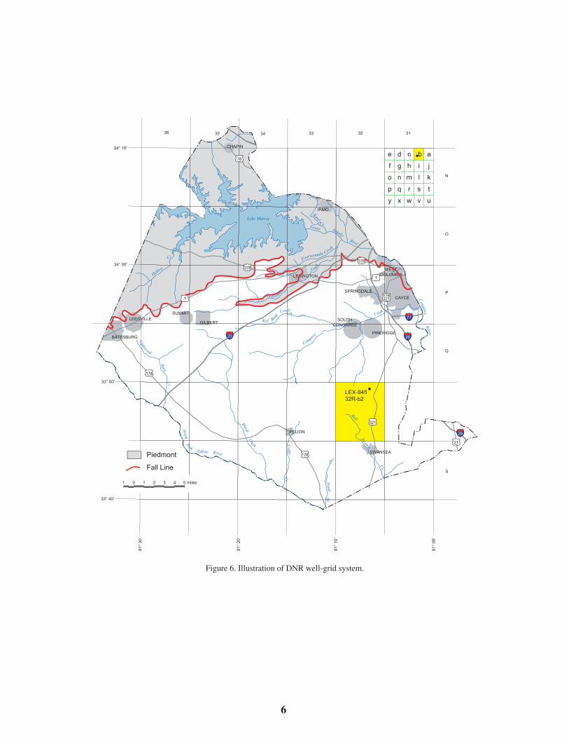
DNR uses a grid system and county number for identifying and locating wells. Each grid division corresponds to 5 minutes of latitude and 5 minutes of longitude. A number signifies the longitude grid, (ex. 32) and an upper-case letter signifies the latitude grid (ex. R). To further define the well location, the 5-minute grid is divided into twenty-five 1-minute latitude-longitude grids represented by the lower-case letters a through y. Wells in a 1-minute grid are numbered consecutively as their records are obtained. For example, the grid number for well LEX-845 would be 32R-b2, wherein 32R represents a 5-minute grid, the letter b represents a 1-minute grid within the 5-minute grid, and the number 2 is the second well inventoried for that particular 1-minute grid (Fig. 6). County numbers are assigned consecutively as well data are obtained.
6
Figure 6. Illustration of DNR well-grid system.

�
Figure 7. Generalized geology of Lexington County modified from Maybin and Nystrom (1995).
GEOLOGY Piedmont rocks occupy the upper third of the county and are part of the Carolina Slate Belt (see the generalized geologic map of Lexington County in Figure 7). The Carolina Slate Belt includes Late Proterozoic to Cambrian metavolcanic and meta-sedimentary rocks that have been metamorphosed to the lower greenschist facies and intruded by plutons (Butler and Secor, 1991, in Geology of the Carolinas). The Carolina Slate Belt also contains deformed and undeformed granitic rocks as well as deformed gabbroic rocks, believed to be Carboniferous in age. The deformational history of these rocks has created complex fracture zones that form the conduits for water in
the Piedmont. Weathered bedrock (saprolite) overlies the crystalline rocks and ranges in thickness from 0 to 100 ft. Saprolite typically is the recharge zone for the underlying fractures that compose the Piedmont aquifer system. It consists of sandy clay, has high porosity but relatively low permeability, and typically is cased off when encountered during drilling.
The Coastal Plain formations consist chiefly of Cretaceous and Tertiary sediments that lie unconformably on the pre-Cretaceous crystalline rocks of the Piedmont. The unconsolidated Cretaceous sediments consist mostly of fine-to-coarse grained, poorly sorted, quartz-sand beds

8
Figure 8. Peachtree Rock Preserve, a 305-acre preserve owned and protected by the Nature Conservancy, is an example of local silicified sandstone beds in the subsurface of Lexington County.
with laterally discontinuous kaolin-clay lenses. Local silicification of beds has created cement-like sandstone lenses and structures. Peachtree Rock, a 305-acre preserve owned and protected by the Nature Conservancy, is one such example. It is located near Swansea and features a silicified sandstone structure shaped like an inverted pyramid (Fig. 8). It is thought this was the area Tuomey (1848), State Geologist of South Carolina from 1844-1847, referred to as the “Rock House.”
Tertiary sediments believed to be of middle to upper Eocene age lie unconformably on the Cretaceous sediments and typically occur as thin, irregular deposits throughout
the county. Middle Eocene sediments consist of well-sorted, fine-grained sand and have considerably less clay than the underlying unit. Upper Eocene sediments consist of thin units of moderately sorted sand with local clay lenses. Other undetermined Tertiary and surficial deposits are observed irregularly throughout the area. The surficial sand deposits are of significant economic value and are being mined in western areas of the county. The similarity between Tertiary and Cretaceous deposits can inhibit their delineation, and because no laterally continuous confining bed can be ascertained, the sediments are, for the purpose of this report, referred to simply as the Coastal Plain deposits.

�
Combined, these sediments range in thickness from 0 at the Fall Line to more than 500 ft near Swansea. The elevation of the Piedmont bedrock surface (Fig. 9) ranges from about +
450 ft msl at the Fall Line to – 250 ft at the south end of the County. Figure 10 illustrates the wedge of Cretaceous-age and younger sediments of the Coastal Plain formations.
Figure 9. Approximate contours on the bedrock surface in Lexington County.
North Fork Edisto River
Black Creek
Congaree
Creek
Red Bank
Creek
Twelvemile
Fourteenmile Creek
Lower Saluda River
Congaree
Lake Murray
River
Pond Br.
Bull Swamp
Cr.
Rawls Cr.
Lightwood
Knot
Cr.
Hollow
Cr.
Creek
Cedar Cr.
Figure 10. Generalized subsurface geology of Lexington County (modified from Aucott and others, (1987).
�0
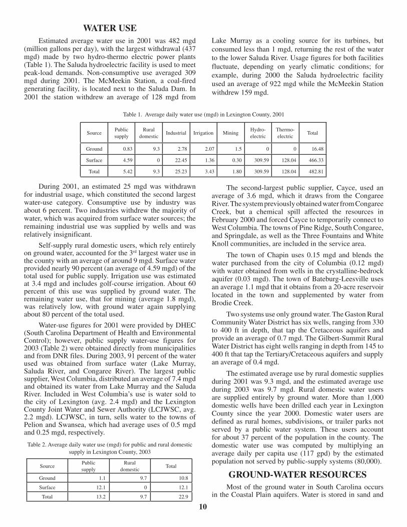
WATER USE Estimated average water use in 2001 was 482 mgd (million gallons per day), with the largest withdrawal (437 mgd) made by two hydro-thermo electric power plants (Table 1). The Saluda hydroelectric facility is used to meet peak-load demands. Non-consumptive use averaged 309 mgd during 2001. The McMeekin Station, a coal-fired generating facility, is located next to the Saluda Dam. In 2001 the station withdrew an average of 128 mgd from
Lake Murray as a cooling source for its turbines, but consumed less than 1 mgd, returning the rest of the water to the lower Saluda River. Usage figures for both facilities fluctuate, depending on yearly climatic conditions; for example, during 2000 the Saluda hydroelectric facility used an average of 922 mgd while the McMeekin Station withdrew 159 mgd.
SourcePublic supply
Ruraldomestic
Industrial Irrigation MiningHydro-electric
Thermo-electric
Total
Ground 0.83 9.3 2.78 2.07 1.5 0 0 16.48
Surface 4.59 0 22.45 1.36 0.30 309.59 128.04 466.33
Total 5.42 9.3 25.23 3.43 1.80 309.59 128.04 482.81
Table 1. Average daily water use (mgd) in Lexington County, 2001
SourcePublic supply
Rural domestic
Total
Ground 1.1 9.7 10.8
Surface 12.1 0 12.1
Total 13.2 9.7 22.9
Table 2. Average daily water use (mgd) for public and rural domestic supply in Lexington County, 2003
During 2001, an estimated 25 mgd was withdrawn for industrial usage, which constituted the second largest water-use category. Consumptive use by industry was about 6 percent. Two industries withdrew the majority of water, which was acquired from surface water sources; the remaining industrial use was supplied by wells and was relatively insignificant.
Self-supply rural domestic users, which rely entirely on ground water, accounted for the 3rd largest water use in the county with an average of around 9 mgd. Surface water provided nearly 90 percent (an average of 4.59 mgd) of the total used for public supply. Irrigation use was estimated at 3.4 mgd and includes golf-course irrigation. About 60 percent of this use was supplied by ground water. The remaining water use, that for mining (average 1.8 mgd), was relatively low, with ground water again supplying about 80 percent of the total used.
Water-use figures for 2001 were provided by DHEC (South Carolina Department of Health and Environmental Control); however, public supply water-use figures for 2003 (Table 2) were obtained directly from municipalities and from DNR files. During 2003, 91 percent of the water used was obtained from surface water (Lake Murray, Saluda River, and Congaree River). The largest public supplier, West Columbia, distributed an average of 7.4 mgd and obtained its water from Lake Murray and the Saluda River. Included in West Columbia’s use is water sold to the city of Lexington (avg. 2.4 mgd) and the Lexington County Joint Water and Sewer Authority (LCJWSC, avg. 2.2 mgd). LCJWSC, in turn, sells water to the towns of Pelion and Swansea, which had average uses of 0.5 mgd and 0.25 mgd, respectively.
The second-largest public supplier, Cayce, used an average of 3.6 mgd, which it draws from the Congaree River. The system previously obtained water from Congaree Creek, but a chemical spill affected the resources in February 2000 and forced Cayce to temporarily connect to West Columbia. The towns of Pine Ridge, South Congaree, and Springdale, as well as the Three Fountains and White Knoll communities, are included in the service area.
The town of Chapin uses 0.15 mgd and blends the water purchased from the city of Columbia (0.12 mgd) with water obtained from wells in the crystalline-bedrock aquifer (0.03 mgd). The town of Bateburg-Leesville uses an average 1.1 mgd that it obtains from a 20-acre reservoir located in the town and supplemented by water from Brodie Creek.
Two systems use only ground water. The Gaston Rural Community Water District has six wells, ranging from 330 to 400 ft in depth, that tap the Cretaceous aquifers and provide an average of 0.7 mgd. The Gilbert-Summit Rural Water District has eight wells ranging in depth from 145 to 400 ft that tap the Tertiary/Cretaceous aquifers and supply an average of 0.4 mgd.
The estimated average use by rural domestic supplies during 2001 was 9.3 mgd, and the estimated average use during 2003 was 9.7 mgd. Rural domestic water users are supplied entirely by ground water. More than 1,000 domestic wells have been drilled each year in Lexington County since the year 2000. Domestic water users are defined as rural homes, subdivisions, or trailer parks not served by a public water system. These users account for about 37 percent of the population in the county. The domestic water use was computed by multiplying an average daily per capita use (117 gpd) by the estimated population not served by public-supply systems (80,000).
GROUND-WATER RESOURCES Most of the ground water in South Carolina occurs in the Coastal Plain aquifers. Water is stored in sand and

��
limestone aquifers that are hydraulically separated by clay and marl confining units. The hydrogeology of the Coastal Plain sediments of Lexington County, however, is complicated by the fact that there are few, if any, laterally continuous clay beds that are sufficiently extensive to be classified as effective confining units. Although these beds cause local water-level differences, the zones above and below the limited confining unit may ultimately respond to pumping. As a result, several water-bearing zones could function as a single aquifer.
As the sediments thicken in the southeastward direction of geologic dip (towards the coast), aquifers and confining units become thicker and better defined. Conversely, aquifers tend to coalesce towards the Fall Line where confining units become thinner and discontinuous. In these updip regions of the Coastal Plain, differentiating aquifers becomes virtually impossible.
WATER LEVELS
Static water level refers to the natural level at which water stands in a cased well that is not being pumped. It is
generally measured from land surface or the top of the well casing.
Water levels ranged from 11 to 205 ft below land surface for all Coastal Plain aquifer tests. Static water levels in the shallow wells near the Fall Line ranged from 11 to 51 ft and from 18 to 205 ft in the deeper wells (175 ft or more).
Three wells in the county have long-term water-level records: LEX-79, LEX-88, and LEX-844. Well LEX-79 is an unused industrial well located in the southeastern part of the county at the old Pennsylvania Sand and Glass Company and is completed in the Cretaceous sand aquifers. Figure 11, adapted from Waters (2003), shows the water level for the period of record from 1966-1981. Discontinuous water levels from 1966 to 1970 are depicted with hollow circles connected by a solid line; a solid line depicts continuous measurements from 1971 to 1981. Water-level fluctuations ranging about 20 ft probably are caused by production wells located nearby and natural seasonal variations.
WELL NUMBER: LEX-79 GRID NUMBER: 33Q-k1LATITUDE: 33°52' 50" LONGITUDE: 81°10' 25"LOCATION: 2 mi southwest of South Congaree, off State Highway 302 and 215 at Pennsylvania Sand and Glass Co.WELL CHARACTERISTICS: 6-inch diameter unused industrial well. Depth: 252 ft.Open interval: 169-252.DATUM: 376 ft above National Geodetic Vertical Datum of 1929.MEASURING POINT: Top of recorder platform, 5.10 ft above land surface datum.PERIOD OF RECORD: 1966-1981.EXTREMES: Highest water level: 100.39 ft below land surface datum, Sept. 8, 1973. Lowest water level: 119.53 ft below land surface datum, Sept. 24, 1981.REMARKS: 1966, 1968-69, lowest water level every 5th day; 1970, mean water levels every 5th day; 1971-81, daily mean water levels.
Figure 11. Well description and hydrograph for well LEX-79.

�2
Well LEX-88 is an unused shallow public-supply well located in downtown Leesville and is completed in the Tertiary and Cretaceous sand aquifers. Figure 12, adapted from Waters (2003), shows the hydrograph for well LEX-88
WELL NUMBER: LEX-88 GRID NUMBER: 37Q-a5LATITUDE: 33°55' 00" LONGITUDE: 81°30' 24"LOCATION: Town of Leesville at the corner of Hall and Greg Streets.WELL CHARACTERISTICS: 16-inch diameter unused public supply well. Depth: 125 ft. Open interval: 41-122 ft.DATUM: 645 ft above National Geodetic Vertical Datum of 1929.MEASURING POINT: Top of recorder platform, 2.20 ft above land surface datum.PERIOD OF RECORD: 1971-1974.EXTREMES: Highest water level: 25.13 ft below land surface datum, April 25, 1973. Lowest water level: 32.21 ft below land surface datum, Dec. 5, 1971.REMARKS: 1971-74, daily mean water levels. Pumping test data provide a transmissivity of 3,200 gpd/ft, a hydraulic conductivity of 65 gpd/ft², specific capacity of 3 gpm/ft, and a pumping rate of 21 gpm.
with continuous measurements from 1971 to 1974. Slight seasonal water level fluctuations with highs occurring in the spring and lows in the fall are observed in addition to evidence of local well interference of 5 to 7 ft.
Figure 12. Well description and hydrograph for well LEX-88.

�3
WELL NUMBER: LEX-844 GRID NUMBER: 32S-b4LATITUDE: 33°44' 45" LONGITUDE: 81°06' 27"LOCATION: Swansea Primary School.WELL CHARACTERISTICS: 2-inch diameter observation well. Depth: 522 ft. Open Interval: 392-502 ft.DATUM: 367 ft above National Geodetic Vertical Datum of 1929.MEASURING POINT: Top of recorder platform, 3.35 ft above land surface datum.PERIOD OF RECORD: 1999-2003.EXTREMES: Highest water level: 69.02 ft below land surface datum, Nov. 15, 1999. Lowest water level: 75.32 ft below land surface datum, Sept. 25, 2002.REMARKS: 1999-2003, daily mean water levels. There were no long-term water level measurements for the rock wells in the county.
Well LEX-844 was drilled during 1997 by DNR and the USGS as part of a geologic study and has been continuously monitored since 1999. This well, completed in the Cretaceous sand aquifers, is part of a Statewide DNR well-monitoring network. The hydrograph in
Figure 13, adapted from Harwell and others (2004), shows a 7-ft water-level decline from 1999 to 2001, presumably a result of the worst drought on record in South Carolina. Recent water levels show a slow recovery.
Figure 13. Well description and hydrograph for well LEX-844.

��
AqUIFER PROPERTIES
Several parameters are used to determine how much water can be withdrawn from an aquifer without rendering undesirable results. This includes, in addition to long-term water-level monitoring, the determination of aquifer transmissivity, hydraulic- conductivity, and storage coefficient.
Pumping tests are used to establish aquifer properties and well hydraulics. Differences can be ascertained with distance below the Fall Line, primarily on the basis of aquifer thickness and depth, water levels, transmissivity, and specific capacity. Most of the pumping tests used for
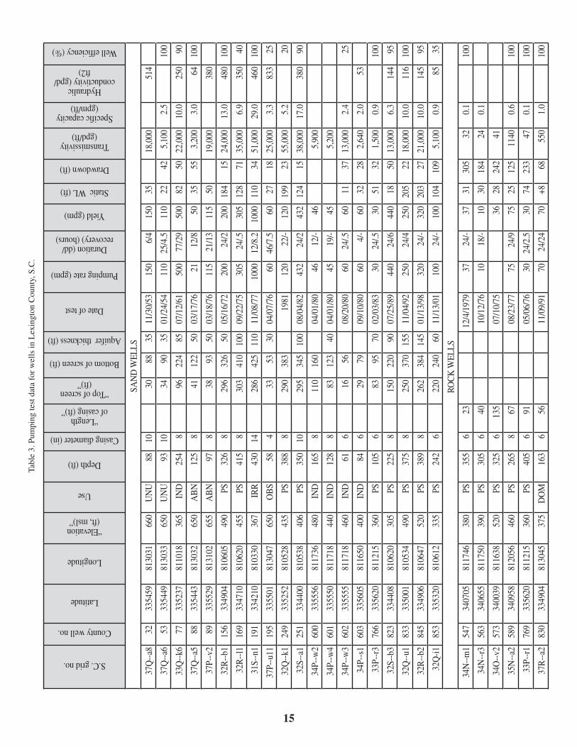
this report are for public-supply wells, for which tests are required by DHEC in order to receive an operating permit. A few of the tests were made at industrial and irrigation wells. A location map of the wells with pumping tests is shown in Figure 14. Of the 20 Coastal Plain pumping tests, 17 were single-well tests in which the discharge and water- level measurements were made at the same well. The remaining tests included the pumped well and at least one observation well. Because most of the tests used for this report involve only the one well, the modified nonequilibrium equation of Jacob (1950) is used. Well and aquifer characteristics of the pumping tests used in this study are listed in Table 3.
81°
00'
81°
10'
81°
20'
81°
30'
33° 50'
34° 00'
34° 10'
36 35 34 33 32 31
N
O
P
Q
S
R
33° 40'
WESTCOLUMBIA
CAYCESPRINGDALE
LEXINGTON
SOUTHCONGAREE
PINERIDGE
PELION
SWANSEA
IRMO
CHAPIN
SUMMIT
GILBERTLEESVILLE
BATESBURG
North Fork Edisto River
Black Creek
Congaree
Creek
Red Bank
Creek
Twelvemile
Fourteenmile Creek
Lower Saluda River
Congaree
Lake Murray
River
Pond Br.
Bull Swamp
Cr.
Rawls Cr.
Lightwood
Knot
Cr.
Hollow
Cr.
Creek
Cedar Cr.
26
378
1
176321
2620
1
378
178
321
178
21
76
77
8853
830
195
3289
589
563547
573
769766
603
601600602
77 249
833
156845
169
823251
191
156
Figure 14. Location of wells for which pumping tests were used in the study.
��
Tabl
e 3.
Pum
ping
test
dat
a fo
r w
ells
in L
exin
gton
Cou
nty,
S.C
.
S.C. grid no.
County well no.
Latitude
Longitude
“Elevation (ft, msl)”
Use
Depth (ft)
Casing diameter (in)
“Length of casing (ft)”
“Top of screen (ft)”
Bottom of screen (ft)
Aquifer thickness (ft)
Date of test
Pumping rate (gpm)
Duration (dd/recovery) (hours)
Yield (gpm)
Static WL (ft)
Drawdown (ft)
Transmissivity (gpd/ft)
Specific capacity (gpm/ft)
Hydraulic conductivity (gpd/
ft2)
Well efficiency (%)
SAN
D W
ELLS
37Q
--a8
3233
5459
8130
3166
0U
NU
8810
3088
3511
/30/
5315
06/
415
035
18,0
0051
4
37Q
--a6
5333
5449
8130
3365
0U
NU
9310
3490
3501
/24/
5411
025
/4.5
110
2242
5,10
02.
510
0
33Q
--k6
7733
5237
8110
1836
5IN
D25
48
9622
485
07/1
2/61
500
77/2
950
082
5022
,000
10.0
250
90
37Q
--a5
8833
5443
8130
3265
0A
BN
125
841
122
5003
/17/
7621
12/8
5035
553,
200
3.0
6410
0
37P-
-v2
8933
5529
8131
0265
5A
BN
978
3893
5003
/18/
7611
521
/13
115
5019
,000
380
32R
--b1
156
3349
0481
0605
490
PS32
68
296
326
5005
/16/
7220
024
/220
018
415
24,0
0013
.048
010
0
32R
--l1
169
3347
1081
0620
455
PS41
58
303
410
100
09/2
2/75
305
24/.5
305
128
7135
,000
6.9
350
40
31S-
-n1
191
3342
1081
0330
367
IRR
430
1428
642
511
011
/08/
7710
0012
/8.2
1000
110
3451
,000
29.0
460
100
37P-
-u11
195
3355
0181
3047
650
OB
S58
433
5330
04/0
7/76
6046
/7.5
6027
1825
,000
3.3
833
25
32Q
--k1
249
3352
5281
0528
435
PS38
88
290
383
1981
120
22/-
120
199
2355
,000
5.2
20
32S-
-a1
251
3344
0081
0538
406
PS35
010
295
345
100
08/0
4/82
432
24/2
432
124
1538
,000
17.0
380
90
34P-
-w2
600
3355
5681
1736
480
IND
165
811
016
004
/01/
8046
12/-
46
5,90
0
34P-
-w4
601
3355
5081
1718
440
IND
128
883
123
4004
/01/
8045
19/-
455,
200
34P-
-w3
602
3355
5581
1718
460
IND
616
1656
08
/20/
8060
24/.5
6011
3713
,000
2.4
25
34P-
-s1
603
3356
0581
1650
400
IND
846
2979
09/1
0/80
604/
-60
3228
2,64
02.
053
33P-
-r3
766
3356
2081
1215
360
PS10
56
8395
7002
/03/
8330
24/.5
3051
321,
500
0.9
100
32S-
-b3
823
3344
0881
0620
305
PS22
58
150
220
9007
/25/
8944
024
/644
018
5013
,000
6.3
144
95
32Q
--u1
833
3350
0181
0534
490
PS37
58
250
370
155
11/0
4/92
250
24/4
250
205
2218
,000
10.0
116
100
32R
--b2
845
3349
0681
0647
520
PS38
98
262
384
145
01/1
3/98
320
24/-
320
203
2721
,000
10.0
145
95
32Q
-i185
333
5320
8106
1233
5PS
242
622
024
060
11/1
3/01
100
24/-
100
104
109
5,10
00.
985
35
ROC
K W
ELLS
34N
--m
154
734
0705
8117
4638
0PS
355
623
12/4
/197
937
24/-
3731
305
320.
110
0
34N
--r3
563
3406
5581
1750
390
PS30
56
4010
/12/
7610
18/-
1030
184
240.
1
34O
--v2
573
3400
3981
1638
520
PS32
56
135
07/1
0/75
3628
242
41
35N
--a2
589
3409
5881
2056
460
PS26
58
6708
/23/
7775
24/9
7525
125
1140
0.6
100
33P-
-r1
769
3356
2081
1215
360
PS40
56
9105
/06/
7630
24/2
.530
7423
347
0.1
100
37R
--a2
830
3349
0481
3045
375
DO
M16
36
5611
/09/
9170
24/2
470
+868
550
1.0
100

�6
Wells in the Piedmont are drilled in fractured bedrock and have properties distinctly different from those drilled in the sand-and-clay formations of the Coastal Plain. Sand wells are constructed with casing having screened intervals to admit water, but rock wells are usually left as open holes so that water flowing through fractures in the bedrock can enter the wells without the use of screens. A relatively small amount of ground water in the Piedmont province is stored in the saprolite and drains downward, by gravity, into fractures and faults in unweathered bedrock. Generally rock wells are low producers, with yields averaging less than 10 gpm; rarely are yields higher. Data from six rock-well pumping tests were analyzed. It should be noted that the equations used to calculate aquifer hydraulics are better suited for porous mediums than for the fractured bedrock of the Piedmont hydrologic system.
Transmissivity
Transmissivity (T) is defined as the rate of flow through a vertical section of an aquifer 1 ft wide and extending the full saturated height of the aquifer under a hydraulic gradient of 1. Transmissivity is expressed in this report in gallons per day per foot of aquifer width and can be calculated using different equations, depending on the type of pumping test performed. It can also be estimated by multiplying the hydraulic conductivity (K), which is expressed in gallons per day per square foot, by the aquifer thickness.
On the basis of 20 sand-aquifer tests, transmissivity values ranged from 1,500 to 55,000 gpd/ft, with a median of 18,000 gpd/ft. Half of the tests were for shallow wells located near the Fall Line with a maximum depth of 160 feet. The highest transmissivity of these tests was 25,000 gpd/ft. The remaining tests provide data mostly from deeper wells located farther from the Fall Line. The deepest of these wells was 425 ft. The highest transmissivity was 55,000 gpd/ft. Table 4 shows the values in comparison. Pumping tests in DNR files indicate median transmissivity values Statewide for the Middendorf Formation (Cretaceous) ranging from 5,000 gpd/ft in Dorchester County to 120,000 gpd/ft in Aiken County, with most values falling between 18,000 and 45,000 gpd/ft.
Table 4. Comparison of transmissivity values (gpd/ft) for 20 sand wells in Lexington County
All wells Shallow wells Deep wells
Average 19,000 9,800 28,000
Median 18,000 5,100 23,000
Range 1,500-55,000 1,500-25,000 5,100-55,000
Transmissivities indicated by six tests of rock wells were so widely ranging as to make analysis useless.
Hydraulic Conductivity
Hydraulic conductivity (K), reported herein as gallons per day per square foot (gpd/ft²), is the quantity of water that will flow through a unit cross section of area per unit of time under a hydraulic gradient of 1 at a specified temperature (Driscoll, 1986). K can be calculated by dividing the transmissivity by the aquifer thickness. Aquifer thickness
is determined from electrical logs or drilling logs; however, wells that only partially penetrate an aquifer will negatively influence the effective thickness. Hydraulic conductivity of an unconsolidated aquifer is affected by the material grain size and sorting, the characteristics of the pore size and connections, and the viscosity of the water. The range for hydraulic conductivity at the sand wells tested in Lexington County is 50 to 830 gpd/ft², with a median of 250 gpd/ft² (Table 5). These K values fall within the range for aquifers composed of silty sand (1 to 104 gpd/ft²) as described by Freeze and Cherry (1979). There was no significant difference in median values between the shallow and deep wells, 220 and 250 gpd/ft², respectively. Statewide average hydraulic-conductivity values for the Middendorf (Cretaceous) aquifer range from 200 gpd/ft² in Charleston and Dorchester Counties, to 1,200 gpd/ft² in Orangeburg County (Newcome, 1997).
Table 5. Comparison of hydraulic-conductivity values (gpd/ft²) for aquifer tests in the Coastal Plain of Lexington County
All wells Shallow wells Deep wells
Average 290 310 270
Median 250 220 240
Range 50-830 50-830 85-480
Storage Coefficient
Storage coefficient (S) is related to the volume of water the aquifer releases from or takes into storage per unit surface area of the aquifer per unit change in head. S is a dimensionless term, and typical values are between 0.3 and 0.03 for water-table aquifers and between 0.005 and 0.0005 for artesian aquifers. Values from 0.03 to 0.005 indicate conditions that are neither truly water table nor artesian (American Water Works Association, 1983). Storage coefficients were calculated for 6 of the 20 sand-aquifer tests, and 3 of these fall within the range of neither being truly a water-table nor an artesian aquifer.
WELL HYDRAULICS
Well Yields
A well’s yield is the volume of water produced by either pumping or free flow and is usually measured in gallons per minute. Pumping tests are commonly used to determine the yield a well can sustain during an established period of time.
Yields for the Coastal Plain pumping tests ranged from 20 to 1,000 gpm. Wells just south of the Fall Line in Lexington County typically produce the lower yields because of thin Coastal Plain sediments and lack of available drawdown. Yields from the upper (shallower) and lower (deeper) sections of the Coastal Plain in the county range from 20 to 150 gpm and 100 to 1,000 gpm, respectively. The median yield for the shallower wells is 60 gpm. The median yield for wells in the southern and southeastern sections of the county is 380 gpm, owing to an increase in aquifer transmissivity and available drawdown.
Yields for the rock-well tests ranged from 8 to 200 gpm. It is only rarely that a rock well produces as much as 200 gpm; it is most likely the well has intercepted several

��
water-yielding zones. Rock-well records in Greenville County (Mitchell, 1995), and Kershaw and Richland Counties (Newcome, 2002 and 2003) show that rock wells generally produce less than 10 gpm.
Specific Capacity
Specific capacity (Q/s) is the number of gallons per minute a well produces for each foot of drawdown, or lowering of the water level. It can be determined by dividing the rate of discharge (Q) by the water-level drawdown (s) after a specified amount of time, usually 24 hours.
Specific-capacity values for the sand-aquifer tests (Table 3) ranged from 0.9 to 29 gpm/ft . Specific capacities of the rock wells tested did not exceed 1 gpm/ft. Potential yields of the wells tested can be estimated by multiplying the amount of available drawdown (distance between static water level and top of the screen or the top of the fracture zone in rock wells) by the specific capacity.
Well Efficiency
Well efficiency is the ratio of the measured specific capacity to the calculated specific capacity of a 100–percent efficient well. A well is said to be fully efficient if the water level in the well measures the same as the water level outside the well. The larger the difference in water levels, the less efficient the well, which has significant economic bearing in that the less-efficient wells cost more to operate. Proper well design and development produce higher efficiencies. Ideal specific capacity is about 1/2000 of the transmissivity. Well efficiency was calculated for 15 of the 20 sand wells with pumping tests. The average well efficiency was around 75 percent and ranged from 20 to 100 percent.
WELLS
Public-Supply Wells
Three major public-supply water systems in Lexington County; Chapin, Gaston Rural Water District, and Gilbert-
Summit Water District, obtain all or part of their water from wells. In addition, there are several smaller systems, such as trailer parks and subdivisions, that also use ground water. Wells for public supply typically are drilled to provide the maximum amount of water possible.
Most public-supply wells are 6 to 10 inches in diameter and equipped with up to 50-horsepower vertical turbine or submersible pumps. The wells generally are 50 to 400 ft deep; those near the Fall Line usually are less than 150 ft deep. Yields range from 5 to 500 gpm. The shallowest water levels reported are less than 10 ft below the land surface, the deepest nearly 300 ft. Most are less than 100 ft.
Irrigation and Industrial wells
Irrigation and industrial wells are constructed with 8- to 14-inch casing and equipped with up to 150-horsepower vertical turbine or submersible pumps. Well depths for both uses range from around 50 to 1,000 ft but are typically between 100 and 450 ft.
Yields for the irrigation wells in the county range from 20 to 1,000 gpm, with static water levels that range from 9 to 138 ft below land surface. Most water levels are less than 75 ft. Yields for industrial wells range from 3 to 650 gpm, and static water levels range from 22 to 160 ft below land surface. The most productive wells are in the southeastern part of the county.
Domestic Wells
Sand Wells
The majority of the sand wells drilled in 2001 were constructed with 4-inch diameter PVC casing, ranged in depth from 30 to 288 ft, and were fitted with ½- to 1½-horsepower submersible pumps. The median depth of 647 wells was 122 ft, and well yields ranged from 0.1 to 200 gpm, with a median of 12 gpm. Figure 15 shows the construction typical of domestic wells.
Figure 15. Typical well construction of rock and sand wells in Lexington County (modified from Mitchell, 1995)

�8
Typically, yields from domestic wells are representative of household or lawn-irrigation needs, usually 20 gpm or less, rather than by what either the aquifer or the well is capable of producing. Static water levels usually are within 30 ft of the land surface. These wells generally are capable of producing 12 to 25 gpm. Wells with little available drawdown are susceptible to drought effects. Environmental stresses that trigger an increased demand for water can cause water levels to drop below the pump setting, which prompts the well owner to assume he has a dry well. In many cases, lowering the pump will solve the problem; however, lowering the pump into the screened section of the well can cause turbulent flow, sand intrusion, and iron precipitation, and result in deteriorating well performance.
The deepest water level recorded for a sand-well was 208 ft below land surface in the south-central part of the county, just north of Pelion. Several of the static water levels were 150 ft or deeper below land surface. Such deep static water levels are common in counties bordering the Fall Line in South Carolina. In Richland County, the deepest water level reported for domestic wells drilled during 2001-02 was 235 ft below land surface for a 278-ft well, (Newcome, 2003). See Table 6 for ranges and medians of static water levels and yields of sand wells.
Table 6. Static water levels and yields for more than 500 sand wells drilled in Lexington County in 2001
Well depth (ft)
No. of wells Water-levelrange (ft)
Medianwater level
(ft)
Yield range (gpm)
Median yield(gpm)
0-100 192 2 - 80 30 4-200 14
101-200 241 3 - 163 83 0.1-100 12
201-300 76 45 -208 150 10-100 12
The available drawdown of a well is an important determinant for how much the well can produce. Multiplying the available drawdown by the specific capacity provides the maximum available yield. The range of available drawdown for all sand wells was 20 to 175 ft, and the median available drawdown was 28 ft. Wells were screened from depths of 20 to 288 ft. The median for the top of the screen setting was 100 ft; the bottom was 120 ft. More than 99 percent of the wells used 20 ft of screen.
Rock Wells
Domestic rock wells drilled in 2001 ranged in depth from 105 to 1,005 ft, were constructed with 6¼-inch PVC casing and equipped with ¾- to 1½-horsepower submersible pumps. The median depth for 321 wells was 305 ft. Figure 15 shows the construction typical of domestic rock and sand wells.
Typically, the driller estimates well yields. Domestic rock-well yields range from less than 1 to 200 gpm, with a median of 10 gpm. Dry holes are a fairly common occurrence. Rock wells are cased through sediments and saprolite (weathered bedrock that characteristically possesses high porosity but low permeability) and completed as open
holes with no screen. The depth cased in open-hole rock wells ranged from 20 (the minimum mandated by law) to 232 ft, with a median depth of 60 ft.
Static water levels ranged from 2 to 125 ft below land surface and had a median of 33 ft. Unlike the sand wells, no large difference could not be detected in water level as related to well depth, but water levels are more likely to be affected by topography differences in the Piedmont. About 90 percent of wells had static water levels between 30 and 40 ft below land surface. See Table 7 for ranges and median of static water levels of rock wells.
Table 7. Static water levels and yields for 231 rock wells drilled in Lexington County in 2001
Wel
l dep
th (
ft)
No.
of
wel
ls
Wat
er-l
evel
ran
ge
(ft)
Med
ian
wat
er le
vel
(ft)
Yie
ld r
ange
(gp
m)
Med
ian
yiel
d (g
pm)
100-200 46 7-62 30 5-50 20
201-300 63 2-77 35 2-150 19
301-400 60 4-83 30 1-200 8
401-500 41 5-74 40 1-100 5
501-600 9 20-47 30 2-39 6
601-700 8 20-125 60 1-5 2
701-800 3 30-60 30 5-50 5
801-900 4 20-30 23 5-20 14
901-1000 1 35-35 35 5-5 5
All depths 235 1-200 33 0-125 10
GROUND-WATER qUALITY
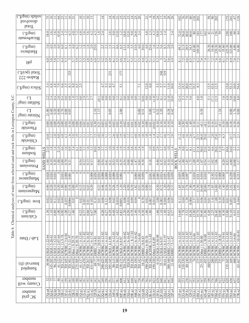
Water-quality data for 52 wells in Lexington County were compiled from DNR well files. The majority of the water samples were analyzed by State and Federal agencies such as South Carolina Water Resources Commission (predecessor to DNR), USGS, or DHEC. Samples analyzed by private labs are designated as Other. Dates for the analyses range from 1961 to 1998.
Sand Wells
Water-quality data were compiled for 35 sand wells (mostly public-supply wells) in Lexington County (Table 8). The locations of these wells are shown in Figure 16. The chemical composition is similar to that of rainwater in that it is very soft (avg. 6 mg/L (milligrams per liter)), fairly acidic (median pH 5.5), and low in dissolved solids (median 18 mg/L). Water containing such low levels of dissolved minerals is indicative of short subsurface residence time and/or nonreactive aquifer material. Counties along the Fall Line contain outcroppings of formations that are conduits for deeper aquifers along the coast and are, therefore, an integral part of the recharge area for the ground-water system of South Carolina’s entire Coastal Plain. Most of
��
SC grid number
County well number
Sampled Interval (ft)
Lab / Date
Calcium (mg/L)
Iron (mg/L)
Magnesium (mg/L)
Manganese (mg/L)
Potassium (mg/L)
Sodium (mg/L)
Chloride (mg/L)
Fluoride (mg/L)
Nitrate (mg/L)
Sulfate (mg/L)
Silica (mg/L)
Radon-222 Total (pci/L)
pH
Hardness (mg/L)
Bicarbonate (mg/L)
Total dissolved
solids (mg/L)
SAN
D W
EL
LS
37Q
-a8
3230
-88
USG
S / 1
-22-
641.
300.
020.
900.
020
1.60
21.0
14.0
0.00
21.0
02.
25.
46.
07.
018
.075
33Q
-k2
7514
5-28
5U
SGS
/ 5-2
6-61
1.10
0.03
0.20
0.01
00.
101.
82.
20.
000.
402.
46.
85.
84.
03.
616
33Q
-k6
7796
-224
USG
S / 7
-12-
610.
800.
120.
100.
010
0.20
1.4
2.0
0.00
0.20
0.4
4.8
5.8
2.0
3.6
1137
Q-a
588
41-1
22U
SGS
/ 2-0
7-64
1.00
0.02
0.30
01.
0021
.08.
00.
200.
402.
07.
97.
34.
043
.064
32R
-i1
141
TD
272
USG
S / 1
1-9-
780.
900.
041.
000.
010
0.80
4.6
4.8
0.00
2.70
0.4
6.6
6.4
6.0
2.4
2333
P-o1
159
TD
105
SCW
RC
/ 3-
6-84
1.00
0.03
50.
900.
008
0.70
1.6
4.3
0.04
0.00
0.0
2.5
5.3
6.1
1.2
1132
S-b1
163
TD
302
USG
S / 5
-21-
970.
270.
0066
0.18
0.00
10.
210.
91.
60.
100.
050.
88.
332
55
1.4
6.3
1632
R-l
116
930
3-41
0O
ther
/ 9-
29-7
51.
600.
020.
000
3.4
5.0
0.00
1.0
8.0
5.7
4.0
4.0
2134
R-t
118
027
5-30
5O
ther
/ 8-
20-7
00
1.70
06.
13.
90.
002.
26.
55.
96.
27.
231
Q-g
118
261
-137
SCW
RC
/ 4-
12-8
30.
220.
020.
150
0.54
0.9
3.1
0.04
0.0
2.5
5.3
1.2
4.8
1031
S-n1
191
374-
470
SCW
RC
/ 6-
17-8
20.
370.
052
0.22
00.
123.
33.
10.
022.
95.
51.
83.
611
35Q
-w1
192
TD
263
SCW
RC
/ 6-
16-8
20.
600.
011
0.43
00.
131.
63.
10.
012.
74.
81.
63.
610
31S-
n219
343
1-48
5SC
WR
C /
6-17
-82
0.47
0.10
20.
200.
000
0.13
3.3
2.7
0.02
2.7
5.9
2.0
4.2
1332
P-f8
242
69-7
7D
HE
C /
8-4-
817.
000.
100.
050
10.0
3.5
0.30
2.10
6.8
25.0
4.3
32P-
w1
247
45-5
5O
ther
/ 10
-9-8
10.
010.
230.
010
0.80
4.8
4.0
0.21
1.13
<0.
15.
21.
832
Q-k
124
929
0-42
5SC
WR
C /
4-12
-83
0.20
0.06
0.46
0.00
00.
543.
73.
60.
030.
04.
75.
22.
52.
414
32R
-e1
250
235-
288
SCW
RC
/ 4-
11-8
30.
270.
121
0.34
0.00
00.
412.
33.
10.
030.
05.
35.
92.
332
S-a1
251
295-
345
USG
S / 4
-1-9
80.
290.
080.
190.
010
0.21
1.0
1.7
0.10
0.05
0.9
8.3
231
4.9
1.5
2.6
1434
P-t1
577
90-1
15SC
WR
C /
4-12
-83
0.40
0.02
0.26
0.00
00.
533.
02.
60.
030.
04.
76.
12.
19.
018
34R
-i1
581
TD
300
SCW
RC
/ 6-
17-8
21.
620.
018
1.14
0.01
02.
193.
44.
00.
023.
25.
58.
612
.021
36P-
u160
813
9-17
5U
SGS
/ 6-9
-97
0.83
0.00
511.
100.
002
0.35
1.9
2.9
0.10
2.00
0.1
5.1
177
4.6
6.5
1.2
1535
R-d
161
2T
D 2
70SC
WR
C /
6-16
-82
2.20
0.08
2.20
00.
543.
54.
00.
020.
05.
413
.518
.023
35Q
-s1
645
TD
130
SCW
RC
/ 6-
16-8
20.
500.
018
0.50
00.
603.
62.
20.
010.
05.
73.
012
.015
35R
-g1
648
TD
230
SCW
RC
/ 8
-17-
820.
780.
090.
390
0.48
2.6
2.7
0.01
3.0
5.3
3.5
9.0
1436
R-j
169
7T
D 1
50SC
WR
C /
6-16
-82
2.40
0.04
1.82
0.00
51.
473.
64.
00.
040.
05.
715
.024
.025
35P-
x373
8T
D 1
42SC
WR
C /
3-6-
841.
100
0.53
0.00
30.
842.
43.
80.
020.
003.
17.
15.
54.
02.
420
31Q
-d4
756
18-2
3D
HE
C /
8-8-
830.
300.
700.
200.
050
0.30
1.9
3.0
0.10
0.31
10.0
4.4
10.0
32Q
-j1
762
190-
298
Oth
er /
6-30
-76
1.60
0.02
0.00
03.
00.
000.
012
.06.
34.
04.
821
33R
-w3
791
TD
240
SCD
NR
/ 9-
1-85
1.80
0.00
70.
520.
043
0.18
1.0
1.8
0.01
0.00
0.0
0.0
5.1
25.0
2.3
832
S-b3
823
150-
220
Oth
er /
8-8-
890.
014
0.00
20.
91.
4<
0.02
<.3
<1.
05.
11.
64.
318
33P-
k183
90-
10U
SGS
/ 4-3
0-98
1.60
3.00
0.30
0.06
50.
402.
94.
10.
100.
320.
25.
55.
35.
218
.024
32P-
f10
840
35-7
3U
SGS
/ 6-9
-97
1.10
0.00
30.
720.
024
0.35
2.7
2.7
0.10
2.20
0.1
5.7
548
55.
62.
417
32Q
-c3
841
30-6
1U
SGS
/ 6-1
1-97
1.40
0.04
81.
200.
051
0.63
4.0
4.6
0.10
0.2
5.7
519
4.5
8.3
1.4
1932
Q-x
184
730
0-34
0D
HE
C /
5-1-
870.
430.
060.
200.
050
0.10
1.0
1.5
0.10
0.38
11.0
11.0
5.6
2.0
2832
P-e4
848
21-6
0D
HE
C /
5-1-
870.
270.
050.
330.
050
0.10
1.4
2.0
0.10
0.42
10.0
10.0
4.9
2.0
2.4
26R
OC
K W
EL
LS
31P-
p120
365
-255
SCW
RC
/ 4-
12-8
314
.60
0.12
1.85
0.05
53.
427.
611
.21.
6012
.413
.48.
149
.372
.010
232
O-x
623
321
0-53
0SC
WR
C /
4-12
-83
7.78
0.04
2.85
0.00
01.
808.
04.
60.
505.
319
.57.
531
.956
.076
32P-
b123
640
-140
SCW
RC
/ 4-
12-8
35.
521.
282.
780.
097
3.45
6.7
3.6
0.40
7.4
20.0
6.6
28.9
40.0
7032
P-f3
237
310
SCW
RC
/ 4-
12-8
310
.20
0.00
41.
800
1.75
8.1
2.6
1.40
5.6
17.8
8.5
34.5
60.0
8033
O-k
125
276
SCW
RC
/ 3-
6-84
15.9
02.
376.
380.
030
1.09
12.1
6.7
0.10
35.5
7.3
65.0
080
128
34M
-y1
543
275
SCW
RC
/ 4-
13-8
335
.70
0.03
13.5
00.
011
1.30
21.8
23.5
0.11
6.0
8.3
8.2
149.
2018
420
234
N-m
154
723
-355
Oth
er /
1-30
-80
39.4
00.
0616
.60
0.01
01.
0738
.068
.0<
0.1
0.30
1.0
7.6
177
34N
-q6
559
455
DH
EC
/ 1-
30-8
031
.80
0.04
20.0
00.
010
0.54
22.0
59.0
<0.
17.
416
234
O-v
119
060
/433
SCW
RC
/ 4-
11-8
36.
480.
012.
180
1.11
6.4
3.1
0.10
5.1
13.5
7.7
26.3
041
5834
P-n1
576
200
SCW
RC
/ 4-
11-8
32.
253.
161.
850.
302
3.02
6.6
2.0
0.16
17.1
43.6
7.2
19.4
021
9035
M-u
258
625
0SC
WR
C /
4-13
-83
28.4
01.
0014
.00
0.42
43.
0628
.025
.00.
2212
.512
.57.
613
9.30
158
202
35N
-r1
615
235
DH
EC
/ 3-
18-8
210
.00
0.10
<50
0.00
011
.07.
5<
0.1
1.24
6.6
43.0
059
35N
-u1
622
75SC
WR
C /
3-19
-81
8.30
0.04
1.40
0.00
50.
205.
76.
30.
103.
86.
135
.60
35N
-u8
629
135-
165
SCW
RC
/ 4-
13-8
333
.80
0.01
9.50
00.
5310
.60.
094.
915
.07.
512
5.30
150
175
35O
-u2
636
169
SCW
RC
/ 3-
13-8
551
.10
0.05
32.
520.
250
4.80
24.0
15.7
0.18
0.00
5.0
53.3
6.9
123.
0016
824
135
P-x1
637
400
SCW
RC
/ 3-
6-84
0.53
0.05
0.60
0.05
010
.00
2.2
2.5
0.10
1.76
10.0
10.0
7.6
4.00
6067
37R
-a2
830
63-1
67SC
WR
C /
10-1
6-91
13.9
10.
164
1.53
0.21
33.
175.
12.
10.
260.
008.
054
.67.
541
.00
6411
8
Tabl
e 8.
Che
mic
al a
naly
ses
of w
ater
fro
m s
elec
ted
sand
and
roc
k w
ells
in L
exin
gton
Cou
nty,
S.C
.

20
Figure 16. Locations of wells for which chemical analyses appear in Table 8.81
° 00
'
81°
10'
81°
20'
81°
30'
33° 50'
34° 00'
34° 10'
36 35 34 33 32 31
N
O
P
Q
S
R
33° 40'
791
the constituents analyzed met State and Federal drinking-water standards; however, most of the samples had low pH, about 17 percent of the samples exceeded the EPA’s (U.S. Environmental Protection Agency) secondary drinking water regulations for manganese, and almost 6 percent of the samples exceeded the MCL (maximum contaminant level) for iron. Samples that exceeded any drinking-water standard are listed in italics in Table 8. For more information on primary or secondary drinking-water standards, local drinking-water standards, or a list of contaminants and their MCL’s, visit the following EPA web address: www.epa.gov/safewater/
Rock wells
Water-quality records were compiled for 17 rock wells in Lexington County (Table 8). The water chemistry is distinctly different from that of the sand wells. Analyses shown in Table 9 depict a median hardness of 41 mg/L, which is closer to being moderately hard by the classification used by Durfor and Becker (1964). Total dissolved solids were higher in the rock wells, with a median of 102 mg/L as compared to 18 mg/L for the sand wells. The median pH was 7.5, close to that of pure water at 25° C (Hem, 1985). As was
true for the sand-well analyses, iron, and manganese were the constituents that exceeded the MCL for drinking-water standards. In addition, the samples from the rock wells had higher concentrations detected for all constituents analyzed.
Table 9. Range of hardness (adapted from Durfor and Becker, 1964)
Hardness (mg/L)
0-60 Soft
61-120 Moderately hard
121-180 Hard
>180 Very hard
RADIONUCLIDES
A major concern for wells located in the Upper Coastal Plain of South Carolina, including Lexington County, is the potential for high levels of radionuclides. Water samples from some wells in the county, and other counties near the Fall Line, have exceeded EPA’s MCL for Radium-226 (226Ra) and Radium-228 (228Ra). High levels were detected in the county as early as the mid-1970’s. In a study by the Clemson University Water Resources Research Institute (1980), wells in and around the town of Batesburg/Leesville
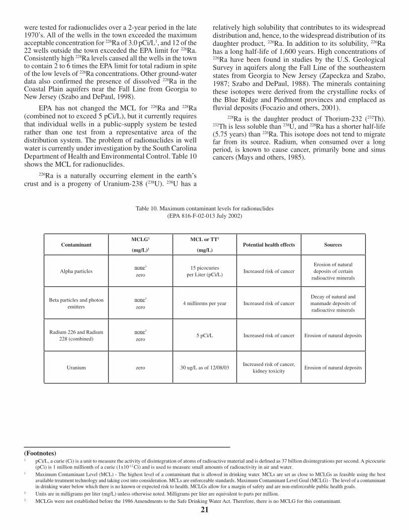
2�
(Footnotes)1 pCi/L, a curie (Ci) is a unit to measure the activity of disintegration of atoms of radioactive material and is defined as 37 billion disintegrations per second. A picocurie
(pCi) is 1 million millionth of a curie (1x10-12 Ci) and is used to measure small amounts of radioactivity in air and water. 1 Maximum Contaminant Level (MCL) - The highest level of a contaminant that is allowed in drinking water. MCLs are set as close to MCLGs as feasible using the best
available treatment technology and taking cost into consideration. MCLs are enforceable standards. Maximum Contaminant Level Goal (MCLG) - The level of a contaminant in drinking water below which there is no known or expected risk to health. MCLGs allow for a margin of safety and are non-enforceable public health goals.
2 Units are in milligrams per liter (mg/L) unless otherwise noted. Milligrams per liter are equivalent to parts per million.3 MCLGs were not established before the 1986 Amendments to the Safe Drinking Water Act. Therefore, there is no MCLG for this contaminant.
ContaminantMCLG�
(mg/L)2
MCL or TT�
(mg/L)Potential health effects Sources
Alpha particlesnone3
zero15 picocuries
per Liter (pCi/L)Increased risk of cancer
Erosion of natural deposits of certain
radioactive minerals
Beta particles and photon emitters
none3
zero4 millirems per year Increased risk of cancer
Decay of natural and manmade deposits of radioactive minerals
Radium 226 and Radium 228 (combined)
none3
zero5 pCi/L Increased risk of cancer Erosion of natural deposits
Uranium zero 30 ug/L as of 12/08/03Increased risk of cancer,
kidney toxicityErosion of natural deposits
Table 10. Maximum contaminant levels for radionuclides (EPA 816-F-02-013 July 2002)
were tested for radionuclides over a 2-year period in the late 1970’s. All of the wells in the town exceeded the maximum acceptable concentration for 226Ra of 3.0 pCi/L1, and 12 of the 22 wells outside the town exceeded the EPA limit for 226Ra. Consistently high 228Ra levels caused all the wells in the town to contain 2 to 6 times the EPA limit for total radium in spite of the low levels of 226Ra concentrations. Other ground-water data also confirmed the presence of dissolved 228Ra in the Coastal Plain aquifers near the Fall Line from Georgia to New Jersey (Szabo and DePaul, 1998).
EPA has not changed the MCL for 226Ra and 228Ra (combined not to exceed 5 pCi/L), but it currently requires that individual wells in a public-supply system be tested rather than one test from a representative area of the distribution system. The problem of radionuclides in well water is currently under investigation by the South Carolina Department of Health and Environmental Control. Table 10 shows the MCL for radionuclides. 226Ra is a naturally occurring element in the earth’s crust and is a progeny of Uranium-238 (238U). 238U has a
relatively high solubility that contributes to its widespread distribution and, hence, to the widespread distribution of its daughter product, 226Ra. In addition to its solubility, 226Ra has a long half-life of 1,600 years. High concentrations of 226Ra have been found in studies by the U.S. Geological Survey in aquifers along the Fall Line of the southeastern states from Georgia to New Jersey (Zapeckza and Szabo, 1987; Szabo and DePaul, 1988). The minerals containing these isotopes were derived from the crystalline rocks of the Blue Ridge and Piedmont provinces and emplaced as fluvial deposits (Focazio and others, 2001). 228Ra is the daughter product of Thorium-232 (232Th). 232Th is less soluble than 238U, and 228Ra has a shorter half-life (5.75 years) than 226Ra. This isotope does not tend to migrate far from its source. Radium, when consumed over a long period, is known to cause cancer, primarily bone and sinus cancers (Mays and others, 1985).

22
SURFACE-WATER RESOURCESRIVERS OF LEXINGTON COUNTY
Three major rivers drain Lexington County. They are the Saluda in the north, which carries discharge from Lake Murray, the Congaree in the east, and the North Fork Edisto in the south. The annual mean flows of the three rivers are depicted in Figure 17. Seasonal variability of unregulated streams typically is represented by higher
flows in the winter months and lower flows in the summer months. Although there is usually more rainfall in the summer, evapotranspiration is also higher and results in reduced streamflow. Streams with regulated flows, such as the lower Saluda River, exemplify hydropower demands and do not necessarily reflect local precipitation. Variations in monthly mean streamflows for the Saluda, Congaree, and North Fork Edisto Rivers are shown in Figure 18. The USGS operates four streamflow gaging stations on these rivers, and their locations are shown in Figure 19.
Figure 17. Annual mean streamflow for the period of record for the Congaree, Saluda, and North Fork Edisto Rivers. Streamflow data can be obtained from the DNR website, www.dnr.state.sc.us/water/hydro/ or the USGS website, www.waterdata.usgs.gov/sc/nwis.
Figure 18. Monthly mean streamflow for the period of record for the Congaree, Saluda, and North Fork Edisto Rivers.

23
The Congaree River near Columbia has the highest annual mean streamflow, 8,946 cfs (cubic feet per second), and the North Fork Edisto River near Orangeburg has the lowest
Figure 19. Locations of USGS streamflow gaging stations on the lower Saluda, Congaree, and North Fork Edisto Rivers.
at 766 cfs. Other streamflow statistics such as minimum and maximum daily streamflow for period of record, percent of flow exceedance, and drainage area are shown in Table 11.
Station ID
Minimum daily mean flow (cfs)
for period of record
Annual mean (cfs)
Maximum daily mean
flow (cfs) for the period of
record 90-
perc
ent
exce
edan
ce
50-
perc
ent
exce
edan
ce
10-
perc
ent
exce
edan
ce
Dra
inag
e ar
ea (
mi²
)
Peri
od o
f re
cord
for
th
is r
epor
t
02169000 Saluda River nr Columbia.
12 (7/13/30) 2,794 63,300
(10/2/29) 414 1,910 6,240 2,520 1925-2002
02168504 Saluda R.
below Lake Murray Dam
155 (9/24/89) 2,467 21,800
(1/16/95) 436 1,550 5,790 2,420 1989-2002
02169500 Congaree R.
nr Cola.
662 (10/18/54) 8,946 150,000
(10/11/76) 2,880 6,580 16,100 7,850 1940-2002
02173500 North Fork Edisto R.
113 (8/13/02) 766 8,850
(9/18/45) 367 662 1,270 683 1939-2002
Table 11. Flow statistics for USGS stream gage 02169000, lower Saluda River near Columbia; stream gage 02168504, Saluda River below Lake Murray Dam; stream gage 02169500, Congaree River near Columbia; and stream gage 02173500, North Fork Edisto River at Orangeburg

2�
Saluda River
The Saluda River flows approximately 10 miles from the Lake Murray Dam before it joins the Broad River to form the Congaree River. In 1991, the South Carolina State Legislature designated the lower Saluda as a State Scenic River; however, comprehensive planning had begun in 1988 by the South Carolina Water Resources Commission (presently part of DNR) and South Carolina Department of Parks, Recreation and Tourism. This 10-mile reach, managed by DNR, is recognized as an outstanding recreational resource and is classified as a “Trout, Put, Grow and Take” (TPGT) river. All other water bodies within this watershed are classified as Freshwater. The temperature of the water entering the river from the bottom of Lake Murray is approximately 52ºF and allows for trout and striped bass fishing, which is unusual this far south and at an elevation of less than 300 ft above sea level. Large whitewater rapids ranging from class II to class V, along with strong currents, provide paddling opportunities usually found in the mountains. The rocky area at Riverbanks Zoo is a popular sunbathing and kayaking spot.
Flow in the Saluda is regulated by Lake Murray Dam, which was constructed to provide hydroelectric power. The USGS and DNR operate and publish stage data for two stream gages on the Saluda River. Station 02168504
is located immediately below the dam and has 13 years of record and Station 02169000, which is located farther downstream near Columbia, has 76 years of record.
The average annual flow (for the 13-year period of record) downstream from Lake Murray (USGS station 02168504) is 2,467 cfs and can vary from 155 to 21,800 cfs. The average annual flow (for the 76-year period of record) for the station near Columbia (USGS station 02169000) is 2,794 cfs and can vary from 12 to more than 62,000 cfs. Because of the difference in length of records, streamflow statistics will differ slightly. Other flow statistics for these stations are listed in Table 11. Two tropical storms moved through the basin in late September of 1929. As a result, a peak flow of 67,000 cfs was recorded on the Saluda River near Columbia on October 2, 1929.
The flow-duration curve for the Saluda River (Fig. 20) was constructed by the USGS and characterizes the hydrology of the stream with respect to time. Typically flows between 0- and the 10- percentile indicate very dry hydrologic conditions while flows between the 90- and 100-percentile indicate very wet hydrologic conditions. Likewise, flows between the 25- and 75-percentiles are typical of normal hydrologic conditions. The 7Q10 minimum flow requirements employed by DHEC are included in the figure.
Figure 20. Flow-duration curve for the Saluda River near Columbia (1925-2001).
2�
The Saluda River watershed (03050109-210) is located in Lexington and Richland Counties and consists of the Saluda River and its tributaries from the Lake Murray Dam to the river’s confluence with the Broad River at Columbia. Major creeks include Rawls Creek, Lorick Branch, and Kinley Creek, all draining south from Irmo, and Twelvemile Creek, which accepts drainage from Long Creek and Juniper Creek near the town of Gilbert, then flows east through the town of Lexington before accepting drainage from Fourteenmile Creek. All water bodies other than the Saluda River (TPGT) are classified as FW.
DHEC operates 9 water-quality monitoring stations in this watershed. For the 5-year Watershed Water Quality Analysis (WWQA) 1997-2001 published by DHEC, aquatic life was partially supported at 5 of the stations, primarily based on macroinvertebrate data. The remaining stations all fully supported aquatic-life uses. Of the eight stations monitored for recreational use, half were not supported owing to fecal-coliform bacteria infractions. Two of the stations partially supported recreational uses, also because of fecal-coliform bacteria infractions, and the remaining two stations fully supported recreational use.
Pursuant to Section 402 of the Clean Water Act (CWA), the National Pollutant Discharge Elimination System (NPDES) was created in 1972. The authority to authorize and administer the program in South Carolina was given to DHEC in 1975. In order to discharge wastes such as those from wastewater treatment facilities, cooling water from industries, and stormwater discharges associated with municipalities, industries or construction sites, an NPDES permit is required and must be approved by DHEC. These permits allow for effluent limitations on certain pollutants, pollutant monitoring and reporting criteria, operating conditions and Best Management Practices to help reduce the pollutant load. Calculations based on Total Maximum Daily Loads (TMDL) and Waste Load Assimilations (WLA) of a water body, coupled with water-quality monitoring are used to determine permit limits.
Fourteen NPDES permits are authorized for the Saluda River watershed (03050109-210); nine discharge to the Saluda River, and the remaining permits authorize discharge to the river’s tributaries. There are five industrial NPDES permits for the Saluda River. One major industrial permit was deactivated in June 2004; the others include two major and two minor industrial permits. Additionally, there are four minor domestic permits with a cumulative discharge of 2.69 mgd. Other receiving streams include Lorick Branch (permitted flow unknown), Kinley Creek (permitted flow unknown), Twelvemile Creek (flow 1.95 mgd), Fourteenmile Creek (flow 0.294 mgd), and Stoop Creek (flow 2.0 mgd).
The city of West Columbia has a surface-water intake along the Saluda River that is used for public water supply. Regulated capacity is 6.0 mgd, with a total pumping capacity of 13.0 mgd (DHEC, 2004c).
Congaree River
The Congaree River is formed by the confluence of the Saluda and Broad Rivers at Columbia and runs 11.5 miles south-southeast along the eastern boundary of Lexington County. The Lexington County reach of the Congaree River upstream from the Granby Lock and Dam contains many shoals and rocky outcrops. There is a landlocked population of striped bass in the Santee-Cooper lakes (Lake Marion and Lake Moultrie) that migrates upstream in the spring to spawn in these shoals. This habitat provides an excellent fishery. This reach of the Congaree River is also a popular canoeing and kayaking area, with many individual and guided trips during the warm months.
USGS data for one gage on the Lexington County border of the Congaree River (02169500) has flow records since 1939 and more than 100 years of peak-stage record. The average annual flow is 8,946 cfs for the period of record. The peak flow recorded at Columbia was 364,000 cfs on August 27, 1908. This flow resulted in a stage of 39.8 ft on the Columbia gage, or 20.8 ft above the current flood stage of 19 ft. Flood stage has been exceeded in 65 of the past 112 years. Daily meanflow statistics for 62 years of record are listed in Table 11.
The flow-duration curve for the Congaree River (Fig. 21) depicts the percentage of time a daily-flow value (calculated from the period of record) will fall within dry, normal, or wet hydrologic conditions. For example, on the first day of January, flow within the 25th percentile, representing dry hydrologic conditions and shaded in yellow on the graph, should be between 4,000 cfs and 5,500 cfs. Flow in the 25th to 75th percentile, representing normal hydrologic conditions and shaded in green, should fall between 5,500 cfs and about 13,000 cfs. The 75th percentile has flow greater than 13,000 cfs and represents very wet hydrologic conditions. The low-flow 7Q10 for the Congaree River, is 1,630 cfs and is used by DHEC for NPDES permits.
The Congaree River is in the southeastern section of the Saluda River basin and consists of an approximately 50-mile stretch of the Congaree River and its tributaries from the headwaters near Columbia, S.C., to its confluence with the Wateree River near Fort Motte, S.C. There are two watersheds in this basin that include DHEC ambient water-quality stations pertaining to Lexington County: the Congaree River watershed (03050110-010) and the Congaree Creek watershed (03050110-020).
The Congaree River watershed is located in parts of Lexington, Richland, and Calhoun Counties and consists of the Congaree River and its tributaries from the river’s origin near Columbia, S.C., to just downstream of Bates Mill Creek. All water bodies in this watershed are classified as Freshwater.
Two DHEC water-quality monitoring stations located in the Congaree River watershed are on the Congaree River at the Blossom Street Bridge. CSB-001L is located on the

26
Figure 21. Flow-duration curve for Congaree River at Columbia (1940-2001).
Lexington County (west) end of the bridge and is designated as the Saluda River. CSB-001R is located on the Richland County end of the bridge and is designated as the Broad River. These sampling stations are so designated because water from the lower Saluda River runs along the west bank and water from the Broad River runs along the east bank. This separation of flow is most evident after a heavy rain. The Saluda River water on the west side comes from the bottom of Lake Murray and is clear; the Broad River water (east side) is brown with sediment carried from the Upstate.
Information provided by DHEC’s WWQA for the Saluda River basin (2004) reports aquatic-life uses were fully supported at station CSB-001L (Saluda River side of the Congaree); however, aquatic-life uses were not supported at the CSB-001R (Broad River side of the Congaree River) owing to zinc infractions. Recreational use was partially supported at CSB-001L owing to fecal-coliform bacteria infractions and fully supported at CSB-001R.
There are 17 NPDES permits authorized to discharge within the Congaree River watershed; 10 discharge to the
Congaree River, and the remaining systems discharge to tributaries of the river. The largest release, at 100.82 mgd, is from a major industry (Voridian) located in Calhoun County. The second-largest permit is a major domestic release of 60.00 mgd from the city of Columbia, located in Richland County. Within this watershed, Lexington County has 8 of the 17 permitted facilities, 3 of which release their effluent, a total of over 12 mgd, to the Congaree River, and the remaining stations release a combined total of 0.3713 mgd to tributaries of the river.
The city of Cayce has a surface-water intake along the Congaree River that is used for public water supply. Regulated capacity is 9.6 mgd, with a total pumping capacity of 14.4 mgd (2004, DHEC). Average daily water use for the city is 3.35 mgd.
Congaree Creek, an important tributary of the Congaree River, originates about 5 miles southeast of the town of Gilbert and flows northeasterly through the towns of South Congaree, Pine Ridge, and Cayce before eventually draining to the Congaree River. Flow records for a USGS

2�
Figure 23. Monthly mean streamflow for Congaree Creek in Lexington County, S.C.
Figure 22. Annual mean streamflow for Congaree Creek in Lexington County, S.C.
stream-gage station are available for Congaree Creek from 1960 to 1980, and the annual mean streamflow is shown in Figure 22. Mean daily flow for Congaree Creek is 221 cfs. The monthly mean streamflow, shown in Figure 23, is usually high in the spring and low in the summer months (USGS website: http://waterdata.usgs.gov/sc/nwis)
The Congaree Creek watershed lies in the lower central section of Lexington County and includes Congaree Creek and its tributaries, which all drain to the Congaree River. All water bodies in this watershed are classified as Freshwater and include Sixmile Creek, Savana Branch, Red Bank Creek, Congaree Creek, First Creek, and Second Creek.
For the 1997-2001 DHEC WWQA (2004), 10 stations were monitored for support of aquatic life: 8 of these stations fully supported aquatic life, 1 partially supported, and 1 did not support aquatic life. Primary reasons for partial or nonsupport were infractions of dissolved oxygen and total phosphorus. Several of these stations were biological stations and did not monitor for recreational-use support. Of
the 7 stations assessed, 3 fully supported recreational use, 2 partially supported, and 2 did not support recreational uses. Primary reasons for partial support or nonsupport were fecal-coliform bacteria infractions.
There are six NPDES-permitted sites in this watershed that discharge to Red Bank Creek, a tributary to that creek, and to First Creek, Bear Creek, and Sixmile Creek. All permitted flows are either minor domestic or minor industrial types, with the largest release being that of Lexington County Joint Municipal Water and Sewer Commission, with a flow of 0.8 mgd.
North Fork Edisto River
The North Fork Edisto River forms approximately 30 miles of the southwestern boundary of Lexington County. It is an unregulated blackwater river located in the Coastal Plain that is formed by Chinquapin Creek and Lightwood Knot Creek just south of I-20. These waters are popular for boating and fishing.
150
175
200
225
250
275
Mon
thly
Mea
n St
ream
flow
(cfs
)
Congaree Creek Monthly MeanStreamflow (1960-1979)

28
The North Fork Edisto USGS gaging station (02173500) is located in Orangeburg at the U. S. Hwy 301 bridge. The Orangeburg gage has flow records from 1939 to the present and an average annual flow of 766 cfs. Daily mean streamflow statistics based on 62 years of record are listed in Table 11. The North Fork Edisto reached a peak flow of 10,000 cfs, or a stage of 14.7 ft, at this gage in September 1928. Flood stage is 8 ft.
The flow-duration curve for the North Fork Edisto River at Orangeburg (Fig. 24) depicts the percentage of time a daily flow value (calculated from the period of record) will fall within dry, normal, or wet hydrologic conditions. For example, on the first day of January, flow within the 25th percentile, representing dry hydrologic conditions and shaded in yellow on the graph, should be between 540 cfs and about 640 cfs. Flow in the 25 th to 75 th percentile, representing normal hydrologic conditions and shaded in
green, should fall between 640 cfs and about 975 cfs. The 75th percentile flow is greater than 975 cfs and represents very wet hydrologic conditions. The low-flow 7Q10 used by DHEC for setting NPDES permit limits for the North Fork Edisto River is 230 cfs, a value published in the USGS Water-Resources Investigations Report 91-4170, (1987).
Flooding along the Lexington County reach of the North Fork Edisto River occurs mostly in the late winter and spring from January through May. Riparian forests and agricultural lands in this reach bound the river, and response to heavy rain events is slow. Floods develop over a period of several days, and the river may stay above flood stage for a week or longer.
The lower portion of Lexington County lies within all or parts of 5 of the 30 watersheds that compose the Edisto River basin. Along the western border of the county, the confluence of Chinquapin Creek and Lightwood Knot Creek
Figure 24. Flow-duration curve for the North Fork Edisto River at Orangeburg (1939-2000).

2�
forms the North Fork Edisto River. Farther downstream, the Black Creek, Bull Swamp Creek, and other smaller tributaries join the North Fork Edisto River.
The five watersheds are Chinquapin Creek and Lightwood Knot Creek (03050203-010), North Fork Edisto River (03050203-020), Black Creek (03050203-030), North Fork Edisto River (03050203-040), and Bull Swamp Creek (03050203-050), and they contain 14 DHEC ambient water-quality monitoring stations that pertain to Lexington County. Aquatic-life uses were fully supported at 13 of these stations, while 1 did not support aquatic-life uses because of dissolved-oxygen infractions. Recreational uses were fully supported at 9 of the 12 stations analyzed. The remaining stations were either partially supported or not supported owing to fecal-coliform bacteria infractions.
The Chinquapin Creek and Lightwood Knot Creek watershed (03050203-010) lies mostly in Lexington County from the town of Batesburg-Leesville to the headwaters of the North Fork Edisto River. All water bodies are classified as Freshwater. Aquatic-life uses were fully supported at all 4 stations. Recreation use was not supported at 2 of the 3 stations monitored.
There is one NPDES permit site in this watershed for the town of Batesburg-Leesville wastewater treatment plant. This permit is classified as major domestic and discharges to Duncan Creek an average of 2.5 mgd.
The North Fork Edisto River watershed (03050203-020) is located in Aiken and Lexington Counties and consists mostly of the North Fork Edisto River and its tributaries, all classified as Freshwater, from its origin to Black Creek (DHEC, 2004). There are numerous small creeks, branches, and ponds that contribute to the watershed. DHEC has two water-quality monitoring stations in this watershed, both along the North Fork Edisto River. Aquatic-life uses and recreational uses are fully supported at both stations. There are no NPDES permits designated for this watershed; however, there are two surface-water intakes, both by the town of Batesburg-Leesville for Lightwood Knot Creek with a regulated capacity of 2.1 mgd and Duncan Creek with a regulated capacity of 1.2 mgd.
The Black Creek watershed (03050203-030) is located in Lexington County, lies adjacent to the North Fork Edisto River watershed, and consists of the Black Creek and its tributaries, all classified as Freshwater. There are two water quality-monitoring stations in this watershed, and both are located on Black Creek. The upstream site is a biological monitoring station, and aquatic-life uses are fully supported. Downstream, aquatic-life uses and recreational uses are both fully supported. There are no NPDES- permit sites located in this watershed.
The North Fork Edisto River watershed (03050203-040) is located in Lexington, Aiken, and Orangeburg Counties and consists of the North Fork Edisto River south of the town of Pelion to northwest of the town of Livingston. The main tributaries are Black Creek and Bull Swamp Creek. There are two water-quality monitoring
stations, located along the Lexington-Aiken County line on the North Fork Edisto River and along the Lexington-Orangeburg County line. Aquatic-life uses and recreational uses are fully supported at both sites.
The Bull Swamp Creek watershed (03050203-050) is located in Lexington, Orangeburg, and Calhoun Counties and consists mostly of Bull Swamp Creek and its tributaries, all classified as Freshwater. There are three water-quality monitoring stations in this watershed, all in Lexington County and all on Bull Swamp Creek. Aquatic-life uses were fully supported at two of the three stations and Recreational uses were fully supported at all three stations. There is one minor industrial NPDES permit for Boggy Branch.
Finally, the North Fork Edisto River watershed (03050203-060) is located in Orangeburg and Calhoun Counties and consists of the North Fork Edisto River and its tributaries from Bull Swamp Creek to Caw Caw Swamp. All waters are classified as Freshwater. Although no water-quality monitoring stations are located in Lexington County, this watershed represents the rivers and creeks that drain directly from the county and can be indicative of potential water-quality problems. There is one water-quality monitoring station in this watershed along the North Fork Edisto River northwest of Orangeburg. Aquatic-life uses are fully supported, but recreational uses are partially supported owing to fecal-coliform bacteria infractions. No NPDES permits have been issued for this watershed.
LAKE MURRAY
During the Civil War, General Robert E. Lee’s Engineering Corps advanced a proposal for construction of a large waterpower dam at Dreher Shoals on the Saluda River. During the 1920’s, William S. Murray envisioned that the largest waterpower impoundment in the world could be achieved by building a dam at the same site.
In 1927 the Federal Power Commission issued a license to the Lexington Water Power Company to construct a dam and powerhouse on the Dreher Shoals site. Construction began on the dam in the spring of 1927. In August of 1930, the South Carolina General Assembly named the resulting impoundment Lake Murray. Power was first generated on December 1, 1930. Lake Murray was filled to the current full-pool elevation of 358 ft msl in 1933. In 1989 the U. S. Army Corps of Engineers required the erection of a steel wall on the upstream face of the dam. This raised the effective elevation of the dam from 375 ft to 377 ft to prevent overtopping in the “probable maximum flood. ”
The level of Lake Murray varies throughout the year from a minimum of 350 ft in early December to a maximum of about 358 ft at the end of May. This “full” elevation is usually maintained until September or October. The Federal Energy Regulatory Commission (FERC) mandated the present owner and operator of the lake, S.C. Electric and Gas Company, to build a second dam adjacent to the current structure in order to strengthen the dam against earthquake hazards.

30
Figure 25 shows the daily water level of Lake Murray compiled and graphed from October 1, 1996, to September 30, 2002. Levels during this time show drought influences from the most recent and severe drought on record. Lake levels are referenced to mean sea level (msl) and are shown in black. The “rule curve” represents the desired operating lake level year-round. In ideal situations, lake levels should shadow the rule curve; however, when the lake level drops below the curve it is indicative of a shortage of water in the lake. Consversely, when the level rises above the curve, it signifies a surplus of water. The rule curve for Lake Murray is plotted against the actual lake level on Figure 25.
Lake Murray is the largest water body in Lexington County at 51,000 acres (79.69 mi2) and contains in excess of 2 million acre-ft of water when at full pool. Other lakes and ponds in the county have a total surface area of approximately 83 mi2. The Lake Murray dam was the largest earthen dam in the world until the Aswan High Dam was built in Egypt during the mid 1960’s. The Saluda Hydro Plant at Lake Murray Dam has five generators capable of producing a total of 206 megawatts of electrical energy and is primarily used as a facility to produce electrical energy during peak demand. Many times on hot summer afternoons, the lower Saluda River will rise rapidly as water coming through the hydroelectric plant moves downstream.
Since 1993, the Aquatic Nuisance Species Program, operated through DNR, has been treating Lake Murray for the exotic plant species hydrilla. Approximately 5,500 acres were treated with herbicides from 1993 to 2001. During 2003, DNR treated 51 acres by stocking the lake with 64,500 triploid (sterile) grass carp that feed on hydrilla (DNR, 2004). Hydrilla is considered an exotic aquatic plant with long, leafy stems that branch and form thick, floating mats. The plants are not native to the area and they typically grow out of control. Left untreated, they can eventually interfere with surface-water recreational uses such as fishing and boating, as well as obstruct drinking-water intakes and impair water quality.
Recreation and real estate are now important uses of Lake Murray. Several high-profile bass tournaments are held at Lake Murray each year. Sailboat regattas are held from time to time, and pontoon-boat cruising is a popular activity. Lakefront property is of high value, and new development continues at a rapid pace.
Lake Murray lies within the Saluda River/Lake Murray watershed (03050109-190 and -150), the Hollow Creek watershed (03050109-200), and the Little Saluda River watershed (03050109-170). There are 17 DHEC water-quality monitoring stations; 10 of which are in Lexington County, 6 in Newberry County and 1 in Saluda County. Several arms of the lake extend into surrounding counties, notably the Saluda River arm and Bush River arm, both in Newberry County. Aquatic-life uses were fully supported at 8 of the stations. Of the remaining stations, 4 partially supported and 5 did not support aquatic-life uses, primarily owing to pH and total phosphorus infractions. Recreational uses were supported at 14 of the monitoring stations. The other 3 stations either partially supported or failed to support recreational uses owing to infractions of fecal-coliform bacteria.
The Saluda River/Lake Murray watershed (03050109-150) is located in Laurens, Newberry, Saluda, and Greenwood Counties and consists mainly of the Saluda River and its tributaries from Lake Greenwood Dam to the headwaters of Lake Murray. This report is concerned with only 4 of the 12 stations monitored in this watershed and those are in Newberry County along the Bush River and Saluda River arms of Lake Murray. All water bodies within this watershed are classified as Freshwater. From the dam at Lake Greenwood, the Saluda River eventually flows past the town of Silverstreet in Newberry County and becomes the Saluda River arm of Lake Murray.
Aquatic-life uses were not supported at 3 of the 4 sites, owing to pH and total phosphorous infractions. Recreational uses were fully supported at 3 of the 4 sites.
Figure 25. Hydrograph of Lake Murray showing actual lake levels and target lake levels from 1996 to 2002 (adapted from Gellici and others, 2004).

3�
There are two minor and two major domestic NPDES permits along the Bush River, but all are considerably upstream from the target monitoring sites. The city of Newberry has a surface-water intake on the Saluda River southwest of the town of Silverstreet. Regulated capacity is 16.0 mgd.
Several monitoring stations on the Bush River have consistently failed to support recreational uses over the recent years by exceeding fecal-coliform bacteria criteria. Pursuant to section 303 (d) of the Clean Water Act (CWA) implemented by EPA, a TMDL was established in 2001 to determine the maximum allowable pollutant load for this area of the river. The maximum load is dependent on the stream’s assimilative capacity and must be able to maintain water-quality standards.
The Little Saluda River/Lake Murray watershed (03050109-170) lies in Saluda County and consists of mainly the Little Saluda River and tributaries to Lake Murray. All water bodies are classified as Freshwater. Although there are three DHEC water-quality monitoring stations in this watershed, only one station, located on the Little Saluda River arm of Lake Murray at SC 391, is of concern. Aquatic-life uses are not supported owing to infractions of pH and total phosphorus concentrations. There are no NPDES permitted facilities of concern in this watershed.
The Saluda River/Lake Murray watershed (03050109-190) consists of the Saluda River and its tributaries and also includes the majority of Lake Murray. The watershed is located in Newberry, Saluda, Lexington, and Richland Counties. All water bodies within this watershed, including Lake Murray, are classified as Freshwater. DHEC operates 11 water-quality monitoring stations within the watershed and only one station, S-290 Camping Creek, is not located on Lake Murray. Of the stations located on the lake, 6 fully supported aquatic life, 3 were partially supported, and 1 failed to support aquatic life uses. The reasons for partial and nonsupport were due to pH and total phosphorus infractions. Water-quality station S-279, a site located farthest uplake at marker 63 failed to support aquatic-life uses due to pH and total phosphorus excursions. During the DHEC Saluda River basin WWQA for 1993-1997 (published in 1998), this site was characterized by high densities of algae, and was considered one of the most eutrophic sites in large lakes in South Carolina. Eutrophication is a term used to describe a lake’s productivity and is also used to describe the age of a lake. Natural eutrophication of a lake can take thousands of years; however, this process can be accelerated by human activity. Water pollution very often is caused by excessive plant nutrients such as phosphorus, nitrogen, and carbon and can manifest itself through excessive algae blooms and organic matter, macrophyte growth, low dissolved oxygen, and a loss of fish habitat. Water samples taken by DHEC during 2002 for trophic assessment showed the most common problem for Lake Murray was attributable to excessive phosphorus.
Two minor domestic NPDES-permitted sites are within this watershed. Newberry Water and Sewer Authority discharges an average of 0.03 mgd to Camping Creek about a mile upstream from station S-290. Stevens Creek receives
an average of 0.0144 mgd. Recreational uses were fully supported at all sites in this watershed with the exception of a site located on Camping Creek, owing to fecal-coliform bacteria infractions.
Lake Murray supplies surface-water intakes to the cities of Columbia and West Columbia. Columbia has a regulated withdrawal capacity of 55.0 mgd, and West Columbia has a regulated withdrawal capacity of 13.5 mgd.
The Hollow Creek/Lake Murray watershed (03050109-200), which chiefly comprises Caney Branch and Little Creek, drains to the middle portion of Lake Murray. All waters are classified as Freshwater. There is one water-quality monitoring site in Hollow Creek located at the southwestern headwaters of Lake Murray. Aquatic-life uses were partially supported owing to pH excursions, and recreational uses were not supported owing to fecal-coliform bacteria infractions. No NPDES permitted facilities are within this watershed, nor are there any surface-water intakes along the creek.
OTHER LAKES AND PONDS
Smaller lakes and ponds aggregate approximately 2,000 acres of water surface. In 1991 the combined volume of these lakes and ponds was about 12,000 acre-ft (U.S. Army Corps of Engineers, 1991). Some were built to provide waterpower for mills and as town water supplies, and now many of these ponds provide waterfront property for subdivisions. Many small lakes that were popular swimming areas in the 1950’s, 1960’s, and 1970’s are no longer used for recreation. Lakes and ponds throughout the county continue to be an important source of water for livestock and fire suppression. A heavy rainfall event in the Red Bank Creek basin in June of 1994 resulted in dam failures on Red Bank Millpond, Crystal Lake, and Durham Pond. Some of these dams were not rebuilt. Many other small ponds in older subdivisions were drained in the 1980’s as a result of changes in Federal Dam Safety Regulations, and they remain empty because of liability and safety concerns.
SUMMARY Lexington County lies in two physiographic provinces, the Piedmont and the Coastal Plain. The Piedmont province, which contains the northern half of the county, has limited ground-water resources. Water flows in through fissures in the crystalline bedrock, and drilled wells penetrating the fissures commonly produce less than 10 gpm, which is not sufficient for public supply, industry, or irrigation. Most wells are used for domestic supply. Consequently, because of the low yields, large water users are forced to use the surface-water resources that are abundant in the area. Lake Murray, is more than sufficient for most water demands. In addition to Lake Murray, other surface-water resources are the lower Saluda and Congaree Rivers in the northeastern part of the county.
Lexington County used an estimated average of 482.81 mgd of water for 2001. The largest water users were by hydroelectric and thermoelectric facilities (437.63 mgd).

32
Public supply use accounted for about 5 mgd. Surface water resources supplied about 466 mgd and wells supplied about 16 mgd.
The water from rock wells is moderately hard and usually had an alkaline pH of 7.5. Some wells in both of the physiograhic provinces of the county, predominantly in the Coastal Plain, have historical and recent analyses showing excessive concentrations of naturally occurring radionuclides. This is currently under investigation by DHEC.
The Coastal Plain in Lexington County, which is southeast of the Fall Line, has abundant ground-water resources that are generally untapped, especially in the southern part of the county. In 2003, ground water supplied about 7 percent (1mgd) of the total used by public utilities but 100 percent of rural domestic supply, an estimated 9 mgd. Wells near the Fall Line are shallow, 100 ft deep or less, owing to the thin Coastal Plain sediments. Pumping-test data from these shallow wells indicate that they are moderately productive, with a median yield of 60 gpm, a median aquifer transmissivity of 5,100 gpd/ft, and a median specific capacity of 2.5 gpm/ft. Water levels range from 11 to 51 ft below land surface.
Pumping tests of wells in the southern part of the county show the aquifers to be much thicker and more productive there. Aquifer transmissivities from 5,100 to 55,000 gpd/ft have been calculated. Wells are as deep as 500 ft, and yields range from 100 to 1,000 gpm. Specific capacities near 30 gpm/ft have been recorded near the Lexington-Orangeburg County line. Water levels are as shallow as 18 ft and as deep as 205 ft. With adequate design and construction, wells capable of producing much more than 1,000gpm are potentially feasible.
The chemical quality of water in the Coastal Plain aquifers is similar to that of rainwater. Analyses in DNR files show the water to be acidic (pH near 5.5) and extremely low in dissolved solids concentration (<25 mg/L). Of the constituents measured, pH, iron, manganese, and radionuclides were found in places, to exceed the maximum contaminant levels set by the U.S. Environmental Protection Agency.
Lexington County has abundant surface-water resources. Of the 700 mi2 in area, approximately 83 mi2 are covered by lakes and ponds 80 mi2 in Lake Murray.
Lake Murray, the fifth-largest lake in the State, contains more than 2 million acre-ft of water. More than 400 miles of streams drain the county. Data from USGS stream gages are available for the Saluda River, Congaree River, and North Fork Edisto River. Annual mean stream-flows vary from 766 cfs to as much as 8,946 cfs. The highest maximum daily mean flow was 150,000 cfs on October 11, 1976 on the Congaree River gage near Columbia.
The North Fork Edisto River is the only truly unregulated stream in Lexington County. The lower Saluda River is regulated by the Lake Murray Dam, which, in turn, partially affects flow of the Congaree River. All rivers in the county are classified by DHEC as Freshwater (FW), with the exception of the 10-mile stretch of the lower Saluda River from the dam to its confluence with the Broad River. This section, because of its unusual water temperature, is classified as Trout, Put, Grow and Take (TPGT) and supports trout and striped bass fishing.
DHEC maintains an ambient surface-water quality-monitoring network throughout the State. Sample collections, analyses, and written reports are implemented and updated for each watershed on a 5-year rotating basin schedule. These data are analyzed, and significant trends in water quality and a summary of stations that support, partially support, or fail to support aquatic-life uses and recreational uses are published in the Watershed Water Quality Assessment for each basin. In addition to the assessment, a priority list of waters that do not currently meet the State water-quality standards is published biennially.
Data from 52 surface-water quality stations monitored for the Edisto and Saluda River Watershed Water Quality Assessments, 1997-2001 (DHEC, 2004) were included in this report. Aquatic-life uses were fully supported at 34 of these stations, while 10 of the stations were partially supported, and 8 were unsupported. Excursions beyond the criteria set for pH was the primary reason for failed or partial support. Of the 46 surface-water quality stations monitored for recreational uses in the study area, 29 were fully supported, 8 were partially supported, and 9 failed to support the use. Excursions beyond the criteria set for fecal-coliform bacteria were the cause of partial support or nonsupport for recreational uses.

33
REFERENCESAucott, W. R., and Newcome, Roy, Jr., 1986, Selected
aquifer-test information for the Coastal Plain aquifers of South Carolina: U. S. Geological Survey Water-Resources Investigations Report 86-4159, 30 p.
Aucott, W.R., Davis, M.E., and Speiran, G.K., 1987, Geohydrologic framework of the Coastal Plain aquifers of South Carolina: U.S. Geological Survey Water-Resources Investigations Report 85-4271, 7 sheets.
American Water Works Association, 1983, Groundwater – A manual of water supply practices: American Water Works Association, New York, N.Y., 130 p.
Badr, A.W., Wachob, Andrew, and Gellici, J.A., 2004, South Carolina Water Plan (2nd ed.): South Carolina Department of Natural Resources 120 p.
Butler, J.R., and Secor, D.T., Jr., 1991, The Central Piedmont, Chapter 4 in Horton, J.W., Jr., and Zullo, V.A., Geology of the Carolinas: Carolina Geological Society, Fiftieth Anniversary Volume.
Castro, J.E., and Hu, Jun, 1997, Distribution and rate of water use in South Carolina, 1994: South Carolina Department of Natural Resources Water Resources Report 18, 18 p., 1 plate.
Driscoll, F.G., 1986, Groundwater and wells, second edition: Published by Johnson Division, St. Paul, Minn. 1089 p.
Durfor, C.N., and Becker, Edith, 1964, Public water supplies of the largest cities in the United States, 1962, U.S. Geological Survey Water-Supply Paper 1812, 364 p.
Ernst, D.C., 2000, Total maximum daily load (TMDL) Rawls Creek, South Carolina: South Carolina Department of Health and Environmental Control, Bureau of Water.
Focazio, M.J., Szabo, Z., Kraemer, T.F., Mullin, A.H., Barringer, T.H., and DePaul, V.T., 2001, Occurrence of selected radionuclides in ground-water used for drinking water in the United States: A reconnaissance survey, 1998: U. S. Geological Survey Water-Resources Investigations Report 00-4273, 39 p.
Freeze, R.A., and Cherry, J.A., 1979, Groundwater: Published by Prentice-Hall, Inc., Englewood Cliffs, New Jersey, 604 p.
Gellici, J.A., and Badr. A.W., 2004, Lake levels in South Carolina during the June 1998-August 2002 drought: in South Carolina Water Resources Report 34, 49 p.
Guimaraes, W.B., Flood of September 7-9, 1987, in Lexington and Richland Counties in the vicinity of Saint Andrews Road and Irmo, South Carolina, WRI 89-4077, 37 p.
Harwell, S.L., Park, A.D., Hockensmith, B.L., and Gawne, C.E., 2004, Water resources data for South Carolina, 2000-2001: South Carolina Department of Natural Resources Water Resources Report 31, 86 p.
Heath, R.C., 1987, Basic ground-water hydrology: U. S. Geological Survey Water-Supply Paper 2220, 84 p.
Hem, J.D., 1985, Study and interpretation of the chemical characteristics of natural water: U.S. Geological Survey Water-Supply Paper 2254, 263 p.
Jacob, C.E., 1950, Flow of ground water: Chap. 5 in Rouse, Hunter, Engineering Hydraulics: New York, John Wiley & Sons.
Kite, L.E., 1987, Cretaceous and Tertiary stratigraphy of the Gilbert 15-minute quadrangle, Lexington and Aiken Counties, South Carolina: in South Carolina Geology, V. 31, No. 1, p. 17-27.
Maybin, A.H., III, and Nystrom, P.G., Jr., 1995, Generalized geologic map of South Carolina (revised by C.A. Niewendorp 1997): South Carolina Department of Natural Resources Hydrology/Geology Map 1.
Maher, H.D., Sacks, P.E., and Secor, D.T., Jr., 1991, The Eastern Piedmont in South Carolina, Chapter 6 in Horton, J.W., Jr., and Zullo, V.A., Geology of the Carolinas: Carolina Geological Society, Fiftieth Anniversary Volume, p. 93-108.
Mays, C.W., Rowland, R.E., and Stehney, A.F., 1985, Cancer risk from the lifetime intake of Ra and U isotopes: Health Physics, v. 48, p. 635-647.
Michel, Jacqueline, and Moore, Willard, 1980, Sources and behavior of natural radioactivity in Fall Line aquifers near Leesville, South Carolina: Clemson University Water Resources Research Institute Technical Report No. 8, 73 p.
Miller, A., 2001, Total maximum daily load development for Bush River: Stations S-046, S-102 fecal coliform bacteria: South Carolina Department of Health and Environmental Control, Bureau of Water.
Mitchell, H.L., 1995, Geology, ground water, and wells of Greenville County, South Carolina: South Carolina Department of Natural Resources Water Resources Report 8, 66 p. 1 plate.
Newcome, Roy, Jr., 1993, Pumping tests of the Coastal Plain aquifers in South Carolina with a discussion of aquifer and well characteristics: South Carolina Water Resources Commission Report 174, 52 p.
3�
____1997a, Hydraulic conductivity of the principal Cretaceous aquifers in South Carolina, in Contributions to the hydrology of South Carolina: South Carolina Department of Natural Resources Water Resources Report 14, p. 51-54.
____1997b, Well efficiency—its importance and its calculation, in Contributions to the Hydrology of South Carolina: South Carolina Department of Natural Resources Water Resources Report 14, p. 45-47.
____2000a, The 100 largest public water supplies in South Carolina− 2000, South Carolina Department of Natural Resources Water Resources Report 21, 40 p.
____2000b, Results of pumping tests in the Coastal Plain of South Carolina (supplement to Water Resources Commission Report 174): South Carolina Department of Natural Resources Water Resources Open-File Report 8, 44 p.
____2003, Ground-water resources of Richland County, South Carolina: South Carolina Department of Natural Resources Water Resources Report 30, 24 p.
Reihm, Chad, June 2001, South Carolina ambient ground-water quality monitoring network 2000: South Carolina Department of Health and Environmental Control, Bureau of Water, 68 p.
Solley, W.B., Pierce, R.R., and Perlman, H.A., 1998, Estimated use of water in the United States in 1995: U.S. Geological Survey Circular 1200, 71 p.
South Carolina Department of Health and Environmental Control, 1998, Watershed water quality assessment – Saluda basin: Technical Report 005-98, (2nd Ed.), 208 p.
____ 1998, Watershed water quality assessment – Edisto basin: Technical Report 006- 98 (2nd Ed.), 151 p.
____ 2001, Watershed water quality assessment − Broad basin: Technical Report 001-01 (2nd Ed.), 245 p.
____ 2002, Water classifications and standards, S.C. Regulation 61-68: South Carolina Department of Health and Environmental Control, Bureau of Water.
____ 2002, State of South Carolina, Section 303(d) list for 2002: South Carolina Department of Health and Environmental Control, 28 p. http://www.scdhec.gov/eqc/water/html/tmdl.html#303d
____ 2002d, Classified Waters, S.C. Regulation 61-69: South Carolina Department of Health and Environmental Control, Bureau of Water.
____ 2002e, South Carolina well standards, S.C. Reg ulation 61-71: South Carolina Department of Health and Environmental Control, Bureau of Water.
____2003, South Carolina water use report 2001 summary: South Carolina Department of Health and Environmental Control, Bureau of Water, 25 p.
____2004, State of South Carolina, Section 303(d) list for 2004: South Carolina Department of and Health and Environmental Control, 33 p. http://www.scdhec.gov/eqc/water/html/tmdl.html#303d
____2004, State of South Carolina Section 305 (b) Integrated report for 2004 Part II Assessment and Reporting: South Carolina Department of Health and Environmental Control @ http://www.scdhec.gov/eqc/water/pubs/305b.pdf
____2004, Watershed Water Quality Assessment: Saluda River Basin: Technical Report No. 004-04, Bureau of Water, Columbia, S.C. 199 p.
____2004, Watershed Water Quality Assessment: Edisto River Basin: Technical Report No. 005-04, Bureau of Water, Columbia, S.C. 140 p.
____2004, State of South Carolina Monitoring Strategy for calendar year 2004: Technical Report No. 001-04 @ http://www.scdhec.gov/eqc/water/pubs/strategy.pdf
South Carolina Department of Natural Resources, 2004, 2004 aquatic plant management plan @ http://www.dnr.state.sc.us/water/envaff/aquatic/plan.html
South Carolina Water Resources Commission, 1983, South Carolina water assessment: Water Resources Commission Report No. 140, 367 p.
Steinert, T.L., 1989, Magnitude and frequency of low streamflows in South Carolina: South Carolina Water Resources Commission Report No. 166. 179 p.
Tuomey, Michael., 1848, Report on the geology of South Carolina: Columbia, South Carolina, 293 p.
U.S. Army Corps of Engineers, 1991, Inventory of lakes in South Carolina, ten acres or more in surface area: South Carolina Water Resources Commission Report No. 171.
U.S. Department of Commerce, 2000, U.S. Census.
U.S. Environmental Protection Agency, 2002, List of contaminants and their maximum contaminant levels: EPA 816-F-02-013.
____ 2002, Clean water act (Sections 101-607)- http://www.epa.gov/region5/water/cwa.html: U.S. Environmental Protection Agency.
____ 2002, National primary drinking water standards, Title 40-Protection of the Environment, Part 141 - http://www.epa.gov/safewater/mcl.html: U.S. Environmental Protection Agency.

3�
____2002, Setting standards for safe drinking water- http://www.epa.gov/safewater/standard/setting.html: U.S. Environmental Protection Agency.
____ 2002, Storet and Retrieval - http://www.epa.gov/storet/: U.S. Environmental Protection Agency.
United States Geological Survey National Water Summary, 1986 - Ground-water quality, hydrologic conditions and events: U.S. Geological Survey Water-Supply Paper 2325, p. 50-57.
____ NWISWEB Data for South Carolina - http://waterdata.usgs.gov/sc/nwis: U. S. Geological Survey.
Waters, K.E., 2003, Ground-water levels in South Carolina: South Carolina Department of Natural Resources Water Resources Report 26, 300 p.
Zapecza, O.S., and Szabo, Zoltan, 1988, Radioactivity in ground water—a review: U.S. Geological Survey Water-Supply Paper 2325, p. 50-57.