water quality assessment using diatom assemblages and advanced

APPLIED ISSUES

Water quality assessment using diatom assemblagesand advanced modelling techniques

MURIEL GEVREY,* FREDERIC RIMET,† YOUNG SEUK PARK,* JEAN-LUC GIRAUDEL,*

LUC ECTOR † AND SOVAN LEK*

*CNRS-UMR, LADYBIO, Universite Paul Sabatier, Toulouse cedex, France

†Centre de Recherche Public – Gabriel Lippmann, CREBS, Luxembourg, Grand Duchy of Luxembourg

SUMMARY

1. Two types of artificial neural networks procedures were used to define and predict

diatom assemblage structures in Luxembourg streams using environmental data.

2. Self-organising maps (SOM) were used to classify samples according to their diatom

composition, and multilayer perceptron with a backpropagation learning algorithm (BPN)

was used to predict these assemblages using environmental characteristics of each sample

as input and spatial coordinates (X and Y) of the cell centres of the SOM map identified as

diatom assemblages as output. Classical methods (correspondence analysis and clustering

analysis) were then used to identify the relations between diatom assemblages and the

SOM cell number. A canonical correspondence analysis was also used to define the

relationship between these assemblages and the environmental conditions.

3. The diatom-SOM training set resulted in 12 representative assemblages (12 clusters)

having different species compositions. Comparison of observed and estimated sample

positions on the SOM map were used to evaluate the performance of the BPN (correlation

coefficients were 0.93 for X and 0.94 for Y). Mean square errors of 12 cells varied from 0.47

to 1.77 and the proportion of well predicted samples ranged from 37.5 to 92.9%. This study

showed the high predictability of diatom assemblages using physical and chemical

parameters for a small number of river types within a restricted geographical area.

Keywords: backpropagation algorithm, benthic diatoms, Kohonen self-organising map, streamecology

Introduction

The distribution and abundance of the species that

constitute biological communities are influenced by

competition (Schoener, 1989; Eklov, 1997) as well as the

availability of environmental resources that are funda-

mental for growth and reproduction (Di Castri &

Younes, 1990; Chapin et al., 1997). These two concepts,

namely species–species and species–environment rela-

tionships, illustrate the non-linear and complex rela-

tionships that often govern a community and the

difficulties that ecologists confront when trying to

interpret these kinds of data. Limitations of many

modelling methods result in data being reduced to

relatively simple metrics, such as species richness,

which often leads to a loss of valuable information and

ecological reality. Two problems arise, however, when

working with complex data sets, first the necessity to

use methods that take into account non-linear responses,

and secondly the need to include community informa-

tion that can be used to predict ecosystem quality.

The usefulness of efficient mathematical tools in

community ecology is apparent (Giske, Huse &

Fiksen, 1998), and ecologists have used mathematical

approaches such as linear regression (e.g. Ricker,

1975), multiple linear regression (e.g. Oberdorff,

Correspondence: Muriel Gevrey, LADYBIO UMR CNRS –

Universite Paul Sabatier, 118 route de Narbonne, F-31062

Toulouse cedex, France. E-mail: [email protected]

Freshwater Biology (2004) 49, 208–220

208 � 2004 Blackwell Publishing Ltd

Hugueny & Guegan, 1997), canonical correspondence

analysis (e.g. ter Braak, 1986), principal component

analysis (e.g. Grossman, Nickerson & Freeman, 1991)

and multiple dimensional scaling (e.g. Legendre &

Legendre, 2000). However, one of the drawbacks of

these methods is that they do not take sufficient

account of data complexity and non-linearity (Blayo &

Demartines, 1991). Artificial neural networks (ANNs)

are techniques that have been shown to work well

with complex and non-linear datasets (Lek et al., 1995;

Scardi, 1996; Recknagel et al., 1997). ANN methods are

based on transmission of information through con-

nections similar to those that occur in the animal

nervous system. Different kinds of ANN exist, usually

classified as supervised or unsupervised learning (Lek

& Guegan, 2000). The most common types of ANN

used in ecology are supervised multilayer perceptron

neural networks with a backpropagation learning

algorithm (BPN) (e.g. Brosse et al., 1999; Maier &

Dandy, 2000) and unsupervised self-organising maps

(SOM) (e.g. Brosse, Giraudel & Lek, 2001; Micha-

elides, Pattichis & Kleovoulou, 2001). SOM is usually

used for ordination and classification (e.g. Chon et al.,

1996; Lek, Guiresse & Giraudel, 1999), whereas BPN is

commonly used to develop predictive models (e.g.

Clair & Ehrman, 1998; Laberge, Cluis & Mercier,

2000). The aim of this study is to present an ecological

modelling method combining SOM and BPN. The

SOM–BPN combination has been tried in medical

imaging (e.g. Reddick et al., 1997; Glass et al., 2000)

and in electrical engineering (e.g. Srinivasan et al.,

1998) and has given satisfactory results for prediction.

The present study, carried out in the framework of the

European project PAEQANN (Predicting Aquatic

Ecosystem Quality using Artificial Neural Networks,

http://aquaeco.ups-tlse.fr/), used a database of ben-

thic diatom inventories and environmental variables

of headwater streams in Luxembourg.

Methods

Database

As part of the PAEQANN project, epilithic samples

were collected from streams (stream orders one to

three according to Strahler, 1963 and Leopold, Wol-

man & Miller, 1964) in spring and autumn from 1994

until 1997. The data, consisting of 289 samples of

benthic diatoms and environmental variables, were

collected according to French and European standard

sampling methods (Kelly et al., 1998; AFNOR, 2000).

In brief, benthic diatoms were collected in riffle areas

from stones, which are not moved under normal

hydrological conditions, by scraping the upper sur-

face of the stones with a toothbrush. Samples were

directly fixed in 4% formaldehyde solution (Prygiel &

Coste, 2000). Diatom valves, cleaned with concen-

trated hydrogen peroxide (H2O2 40%) to eliminate

organic matter and hydrochloric acid in each sample

to dissolve calcium carbonates were mounted in

Naphrax�. Up to 400 valves were counted and

identified in each sample (Iserentant et al., 1999). An

agglomerative hierarchical clustering analysis

(Ward’s method for linkage and Euclidean distances)

of diatom inventories showed no correlation between

sampling season (spring or autumn) and diatom

assemblages, hence the data were pooled.

The habitats where diatom samples were collected

were characterised using nineteen topographical,

physical and chemical variables: width, slope, distance

from source, water temperature, dissolved oxygen,

conductivity, total phosphorus, pH, NO�3 , NO�

2 , NHþ4 ,

PO3�4 , Na+, Cl), K+, SO2�

4 , biological oxygen demand

(BOD)5, total hardness and carbonate hardness. Some

chemical variables were measured directly at the

sampling site (e.g. pH, conductivity) whilst others

were analysed in the laboratory following standard

procedures (e.g. NO�3 , NO�

2 , NHþ4 , PO3�

4 ). Topograph-

ical parameters (width, slope and distance from

source) were measured on 1/20 000 maps.

A total of 411 diatom taxa were recorded from the

289 samples. Because of the dominance of rare species

(e.g. 50% of the taxa occurred no more than three

times in 289 samples) and to facilitate the work of

managers, the species data-matrix was reduced (see

below).

ANN models

Two ANN algorithms were used to model the

structure of the diatom assemblages: (i) SOM, an

unsupervised neural network, was used to ordinate

diatom assemblages in a two dimensional grid and (ii)

BPN, a supervised neural network, was used to

predict the assemblages classified by SOM.

In brief, SOM, also referred to as a Kohonen neural

network, approximates the probability density func-

tion of the input variables and performs a non-linear

Water quality assessment and diatom assemblages 209

� 2004 Blackwell Publishing Ltd, Freshwater Biology, 49, 208–220

projection of the multivariate data into a two-dimen-

sional space (Kohonen, 1982, 2001). SOM consists of

two layers of neurones (i.e. computational units)

connected by weights (connection intensities): the

input layer is connected to a vector of the input

dataset and the output layer forms a map consisting of

a rectangular grid laid out in several neurones (cells).

During the learning process the weights are modified

to minimise the distances between weight and input

vectors. This results in classifying the input data

according to their similarities and preserving the

connection intensities.

Backpropagation learning algorithm is one of the

most popular ANN algorithms (Rumelhart, Hinton

& Williams, 1986; Lek & Guegan, 2000) as it has the

ability to learn patterns when given training data,

and to generalise results from the training dataset.

BPN is composed of three layers (input, hidden and

output layers) of interconnected processing elements

(neurones) and each neurone is connected with

neurones of the previous layer by weighted links

and activated by the sigmoid transfer function

f(x) ¼ 1/(1 + e)x), where x is input data. During

training the network is designed to compare

expected and calculated values, and to modify

connection weights to reduce the mean square error

(MSE).

A detailed description of both algorithms and their

applications in ecology are given in Chen & Ware

(1999) and Lek & Guegan (2000).

Modelling processes

For the prediction of the diatom assemblages in this

study, SOM was used to give groups of diatom

assemblages and BPN was used to predict these

assemblages. A complete modelling sequence is

constructed following four steps (Fig. 1):

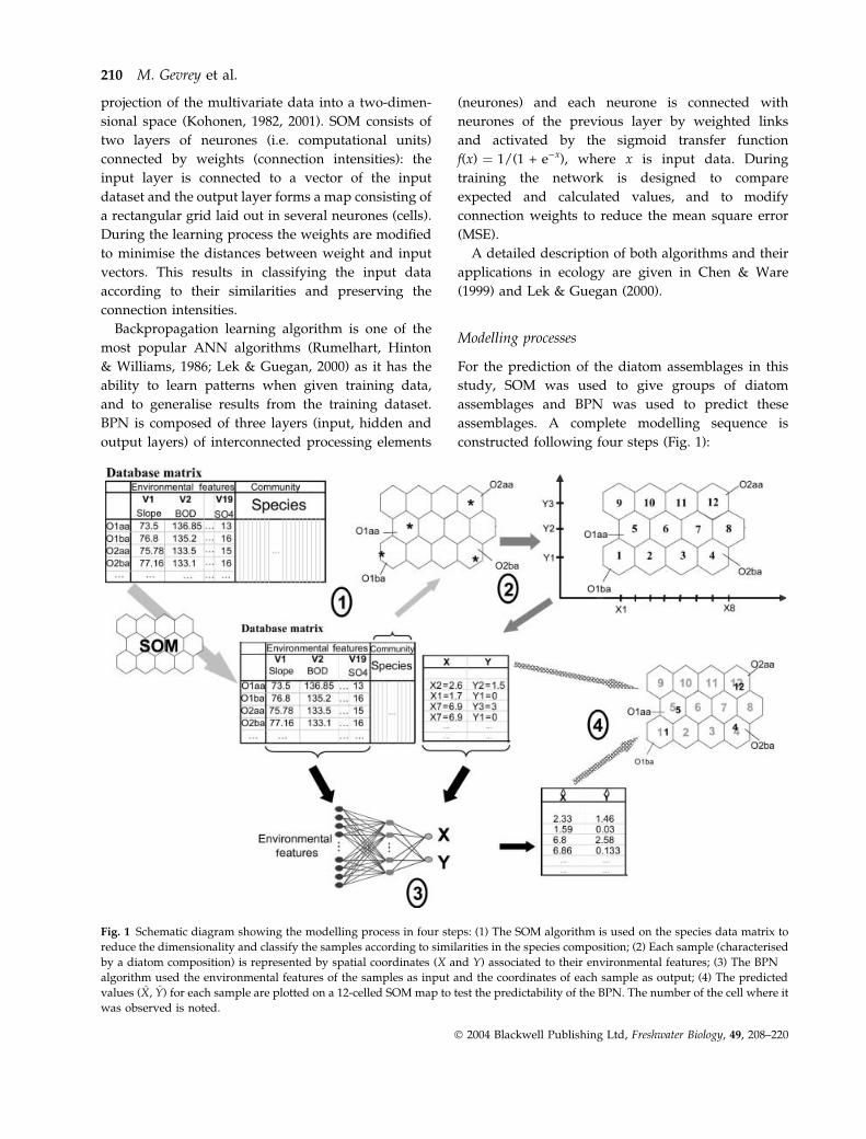
Fig. 1 Schematic diagram showing the modelling process in four steps: (1) The SOM algorithm is used on the species data matrix to

reduce the dimensionality and classify the samples according to similarities in the species composition; (2) Each sample (characterised

by a diatom composition) is represented by spatial coordinates (X and Y) associated to their environmental features; (3) The BPN

algorithm used the environmental features of the samples as input and the coordinates of each sample as output; (4) The predicted

values (X, Y) for each sample are plotted on a 12-celled SOM map to test the predictability of the BPN. The number of the cell where it

was observed is noted.

210 M. Gevrey et al.


(1) First, data dimensions were reduced by elimin-

ating taxa showing low density and/or low occur-

rence by SOM. SOM reduced the diatom assemblage

matrix (density and taxon occurrence) to a number of

assemblages using the connection intensity values

that represent the abundance of each taxon in the

assemblages. Data reduction, using the connection

intensities of the SOM, allowed species with connec-

tion intensities <10% to be discarded. In the final data

matrix, 71 taxa were selected from 411 total taxa for

the ANN models. SOM were then trained again with

densities of 71 taxa to classify different groups of

assemblages based on their species similarities. In

SOM classification, the number of output neurones

(i.e. the map size) is important: if the map size is too

small, differences among assemblages might not be

adequately described, conversely, if the map size is

too big the differences among assemblages become

trivial (Wilppu, 1997). Thus, we trained the network

with different map sizes, and chose the optimum map

size based on the minimum values for quantisation

and topographic errors, which are used to evaluate

the map quality (Park et al. 2003). In this study, a 12-

celled map was used, (i.e. a rectangular map of 4 · 3

cells), with each of the 12 cells considered as repre-

senting a different diatom assemblage.

(2) A SOM map is represented by a two-dimen-

sional lattice, where each point of the grid can be

defined by X and Y coordinates. Each sample is then

characterised by the X and Y coordinates of the centre

of the cell where it has been placed, and by the

original data using the environmental variables. A

new matrix is therefore constructed with, for each

sample, its environmental features and the coordi-

nates of the centre of the cell in which it is observed.

BPN was used to predict the coordinates of the

samples in the SOM with the environmental variables.

Two output neurones were used to predict the X and

Y coordinates of the cell centres of the SOM map. A

Jacknife leave-one-out validation procedure (Efron,

1983; Efron & Tibshirani, 1995), where each sample is

tested using a model trained by all the other

observations, was used to test the predictive quality

of the model. Nineteen environmental variables were

used as input variables in input neurones to predict

the coordinates of the SOM cells (X and Y, i.e. two

output neurones). Thirteen neurones were used in the

hidden layer of the artificial network and the network

converged after 500 iterations according to the best

compromise between bias and variance (Geman,

Bienenstock & Doursat, 1992; Kohavi, 1995).

(3) The estimated X, Y coordinate values of each

sample were plotted on the same SOM map and a

sample was estimated as being well predicted if it was

plotted in the cell area where it had been observed (i.e.

included in the expected samples).

The simulating program in the Matlab environment

that was used for this work is available from the first

author request.

For each cell, two indices were used to assess the

quality of the model:

(1) The total mean square error (MSEt) was calcu-

lated by considering the sum of the abscissa MSE

(MSEabs) and ordinate MSE (MSEord):

MSEt ¼ MSEabs þMSEord

¼PN

i¼1 Xobsi�Xpredi

� �2þ Yobsi

�Ypredi

� �2

Nð1Þ

where N is the number of samples in a cell, Xobs is the

observed abscissa, Xpred is the predicted abscissa, Yobs

is the observed ordinate and Ypred is the predicted

ordinate.

(2) The percentage of well predicted samples (Pwp),

which is defined as the ratio of samples predicted

inside the specific cell and the total number of samples

classified in the cell, varied from 0 (all samples were

predicted outside the cell) to 100 (all samples were

predicted inside the cell) was calculated as:

Pwpð%Þ ¼ n

N� 100 ð2Þ

where n is the number of samples predicted to lie

inside a cell and N is the total number of samples in a

cell. A cell is considered as well predicted if Pwp is

high and MSEt is low (i.e. the samples are inside and

near the centre of the cell).

As SOM placed samples into different cells accord-

ing to their similarities of taxa composition, all

samples in a cell have similar taxa assemblages. To

identify the relations between assemblages and the

cell number the taxa were analysed by their connec-

tion intensities. This was performed using the density

probabilities of each taxon in SOM cells using corres-

pondence analysis (CA) (Hill, 1973) and divisive

hierarchical clustering analysis (DHC) (Kaufman &

Rousseeuw, 1990). Canonical correspondence analysis



(CCA) (ter Braak, 1986) was used to define the

relationship between diatom assemblages and envir-

onmental conditions using the 16 physical and

chemical variables and the 19 relevant diatom taxa

(Table 2) of the groups defined by the CA and DHC.

Results

Diatom assemblages were classified according to the

gradient of species composition on the SOM map,

with each cell corresponding to a specific diatom

assemblage (Fig. 2). The number of samples in each

cell ranged from eight (in cell six) to 39 (in cell nine)

(Table 1).

Using a Jacknife leave-one-out validation procedure

of the BPN, the correlation coefficients between

observed and predicted values of X and Y spatial

coordinates were 0.93 and 0.94, respectively. Most

samples were well located, although some misalloca-

tions were noted in cells three, six, seven and 10

(Fig. 3). The highest MSE and the smallest proportion

of well predicted samples were obtained for these

four cells and relatively small numbers of samples

were found in cells six, seven and 10 (Table 1). The

coexistence of diatom taxa at one sampling site is

controlled by the environmental descriptors. In this

study, cells one, two, five and nine on the left side of

the SOM map are characterised by samples with

higher conductivity, carbonate hardness and pH than

cells four, eight and 12 on the right side of the map.

The influence of geology is also evident, as samples to

the left were from sandstone areas, whilst samples to

Fig. 2 (a) A SOM map of species abun-

dance of 289 samples of diatom assem-

blages from the Luxembourg streams

plotted according to similarities in species

composition. The name of each sample is

represented by an abbreviation ending

with two letters, where the first letter de-

notes sampling area and the second letter

shows if the sample was collected during

spring (p) or autumn (a). The number of

samples in each cell varied from eight to

39 (see also Table 1). (b) A box plot of the

distribution of the samples in the cells of

the SOM map. The tails of the box repre-

sent the maximum and the minimum

values of the number of samples per cell,

and the horizontal line in the box repre-

sents the average value.



the right were dominated by schist. Cells in the

bottom of the SOM map (one, two, three and four)

show higher values of PO3�4 , NO�

2 and BOD5 than

cells nine, 10, 11 and 12, in the upper areas. This

finding indicates that samples in the bottom of the

SOM map are affected by anthropogenic disturbances

such as organic pollution or eutrophication.

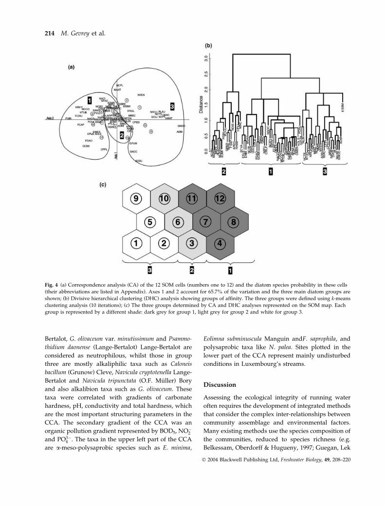
Both CA and DHC analyses showed three main

diatom groups and several subgroups (Fig. 4). The

three main groups were also defined by k-means

clustering analysis. Three main groups of assemblages

were also revealed in the SOM map (as shown in

Table 2). The first group was composed of cells four,

seven, eight, 11 and 12, the second of cells three, six

and 10 and the third of cells one, two, five and nine

(Fig. 4c).

While the samples allocated to a given cell have

similar diatom assemblages, those in neighbouring

cells are less similar, and dissimilarity increases with

distance between cells. Species that have a probability

of presence of over 0.8 are given in Table 2. The

diatom compositions of each cell were clearly related

to their ecology, and in agreement with the observa-

tions of van Dam, Mertens & Sinkeldam (1994). For

example, alkaliphilic taxa such as Amphora pediculus

(Kutzing) Grunow, Cocconeis placentula var. lineata

(Ehrenberg) Van Heurck, Rhoicosphenia abbreviata

(C.A. Agardh) Lange-Bertalot andMayamaea atomus

var. permitis (Hustedt) Lange-Bertalot and alkalibion

taxa such as Gomphonema olivaceum (Hornemann)

Brebisson are located in the left part of the SOM

map (cells one, five and nine). Neutrophilic taxa, such

as Achnanthidium minutissimum (Kutzing) Czarnecki,

G. olivaceum var. minutissimum (Hustedt) Lange-

Bertalot, Navicula gregaria Donkin, Fistulifera saprophila

Lange-Bertalot & Bonik, Nitzschia palea (Kutzing)

W.M. Smith andGomphonema parvulum Kutzing are

found on the right side (cells four, eight and 12)

(Table 2 and Fig. 4). The diatom assemblages also

show a pollution-gradient from the top to the bottom

of the SOM map. For instance, F. saprophila, M. atomus

var. permitis, Eolimna minima Grunow, andN. gregaria

Donkin are a-mesosaprobic to polysaprobic and

eutrophic species and are mainly found in cells one,

two, three and four, whilst A. minutissimum, a com-

mon b-mesosaprobic diatom, is found in high abun-

dance (over 47%) in several other cells (nine, 10, 11

and 12). Hence, the cells at the bottom of the map

correspond to sites with high pollution, whilst the

cells at the top correspond to minimally disturbed or

unpolluted rivers.

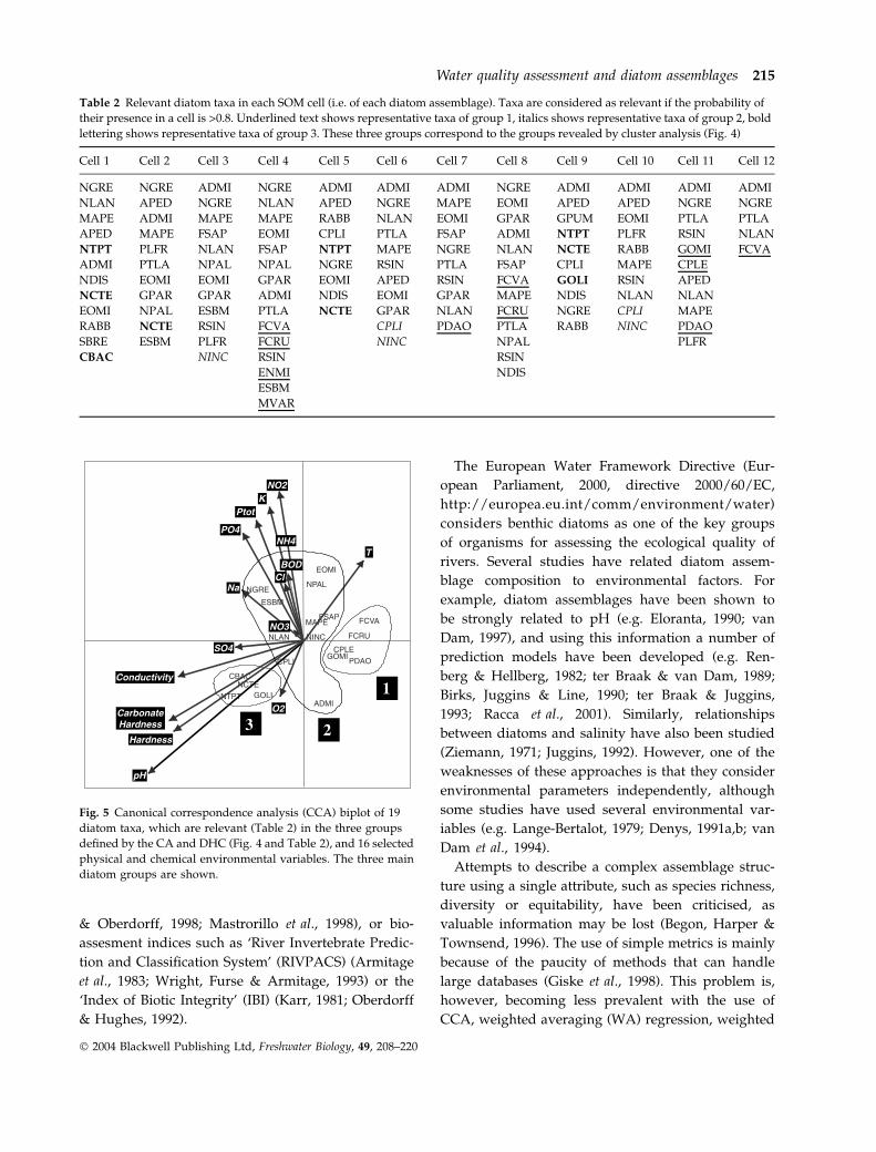
Canonical correspondance analysis (CCA) showed

the relationship between diatom assemblages and

environmental conditions, revealing clear ecological

and physical-chemical gradients (Fig. 5). Ecological,

physical and chemical gradients were clearly defined

and indicated the water quality. According to van

Dam et al. (1994) the species in group one, Fragilaria

capucina Desmazieres ssp. rumpens (Kutzing) Lange-

Table 1 Summary table giving the number of samples (N)

plotted in each cell of the SOM, the total mean square errors

(MSEt), the number of well predicted samples (n) in each cell

(cf. page 211) and the percentage of well predicted samples

[Pwp (%)]

No. of cells N MSEt n Pwp (%)

1 27 0.6988 20 74.1

2 24 0.7316 17 70.8

3 23 1.0607 14 60.9

4 32 0.7802 24 75.0

5 14 0.485 13 92.9

6 8 1.7672 3 37.5

7 11 0.8974 5 45.4

8 27 0.6378 21 77.8

9 39 0.4669 36 92.3

10 16 1.7259 8 50.0

11 36 0.8641 26 72.2

12 32 0.7311 23 71.9

Fig. 3 Predicted results of a leave-one-out validation procedure

of the BPN model. The samples are plotted with their predicted

coordinates. The samples predicted within the corresponding

area were considered as well predicted. Each sample is plotted

using the number of the cell where it was observed. The ob-

served coordinates are represented in the centre of each cell, and

the predicted coordinates are at their precise position on the

map.



Bertalot, G. olivaceum var. minutissimum and Psammo-

thidium daonense (Lange-Bertalot) Lange-Bertalot are

considered as neutrophilous, whilst those in group

three are mostly alkaliphilic taxa such as Caloneis

bacillum (Grunow) Cleve, Navicula cryptotenella Lange-

Bertalot and Navicula tripunctata (O.F. Muller) Bory

and also alkalibion taxa such as G. olivaceum. These

taxa were correlated with gradients of carbonate

hardness, pH, conductivity and total hardness, which

are the most important structuring parameters in the

CCA. The secondary gradient of the CCA was an

organic pollution gradient represented by BOD5, NO�2

and PO3�4 . The taxa in the upper left part of the CCA

are a-meso-polysaprobic species such as E. minima,

Eolimna subminuscula Manguin andF. saprophila, and

polysaprobic taxa like N. palea. Sites plotted in the

lower part of the CCA represent mainly undisturbed

conditions in Luxembourg’s streams.

Discussion

Assessing the ecological integrity of running water

often requires the development of integrated methods

that consider the complex inter-relationships between

community assemblage and environmental factors.

Many existing methods use the species composition of

the communities, reduced to species richness (e.g.

Belkessam, Oberdorff & Hugueny, 1997; Guegan, Lek

Fig. 4 (a) Correspondence analysis (CA) of the 12 SOM cells (numbers one to 12) and the diatom species probability in these cells

(their abbreviations are listed in Appendix). Axes 1 and 2 account for 65.7% of the variation and the three main diatom groups are

shown; (b) Divisive hierarchical clustering (DHC) analysis showing groups of affinity. The three groups were defined using k-means

clustering analysis (10 iterations); (c) The three groups determined by CA and DHC analyses represented on the SOM map. Each

group is represented by a different shade: dark grey for group 1, light grey for group 2 and white for group 3.



& Oberdorff, 1998; Mastrorillo et al., 1998), or bio-

assesment indices such as ‘River Invertebrate Predic-

tion and Classification System’ (RIVPACS) (Armitage

et al., 1983; Wright, Furse & Armitage, 1993) or the

‘Index of Biotic Integrity’ (IBI) (Karr, 1981; Oberdorff

& Hughes, 1992).

The European Water Framework Directive (Eur-

opean Parliament, 2000, directive 2000/60/EC,

http://europea.eu.int/comm/environment/water)

considers benthic diatoms as one of the key groups

of organisms for assessing the ecological quality of

rivers. Several studies have related diatom assem-

blage composition to environmental factors. For

example, diatom assemblages have been shown to

be strongly related to pH (e.g. Eloranta, 1990; van

Dam, 1997), and using this information a number of

prediction models have been developed (e.g. Ren-

berg & Hellberg, 1982; ter Braak & van Dam, 1989;

Birks, Juggins & Line, 1990; ter Braak & Juggins,

1993; Racca et al., 2001). Similarly, relationships

between diatoms and salinity have also been studied

(Ziemann, 1971; Juggins, 1992). However, one of the

weaknesses of these approaches is that they consider

environmental parameters independently, although

some studies have used several environmental var-

iables (e.g. Lange-Bertalot, 1979; Denys, 1991a,b; van

Dam et al., 1994).

Attempts to describe a complex assemblage struc-

ture using a single attribute, such as species richness,

diversity or equitability, have been criticised, as

valuable information may be lost (Begon, Harper &

Townsend, 1996). The use of simple metrics is mainly

because of the paucity of methods that can handle

large databases (Giske et al., 1998). This problem is,

however, becoming less prevalent with the use of

CCA, weighted averaging (WA) regression, weighted

O2

T

pH

CarbonateHardness

Hardness

Conductivity

NO2

PO4

Na

Ptot

SO4

K

ADMI

NGRE

MAPE

EOMI

FSAP

NPAL

NLAN

CPLI

NINC

FCVA

GOMICPLE

PDAO

FCRU

GOLI

ESBM

NCTE

NTPT

CBAC

1

23

NH4

BODCl

NO3

Fig. 5 Canonical correspondence analysis (CCA) biplot of 19

diatom taxa, which are relevant (Table 2) in the three groups

defined by the CA and DHC (Fig. 4 and Table 2), and 16 selected

physical and chemical environmental variables. The three main

diatom groups are shown.

Table 2 Relevant diatom taxa in each SOM cell (i.e. of each diatom assemblage). Taxa are considered as relevant if the probability of

their presence in a cell is >0.8. Underlined text shows representative taxa of group 1, italics shows representative taxa of group 2, bold

lettering shows representative taxa of group 3. These three groups correspond to the groups revealed by cluster analysis (Fig. 4)

Cell 1 Cell 2 Cell 3 Cell 4 Cell 5 Cell 6 Cell 7 Cell 8 Cell 9 Cell 10 Cell 11 Cell 12

NGRE NGRE ADMI NGRE ADMI ADMI ADMI NGRE ADMI ADMI ADMI ADMI

NLAN APED NGRE NLAN APED NGRE MAPE EOMI APED APED NGRE NGRE

MAPE ADMI MAPE MAPE RABB NLAN EOMI GPAR GPUM EOMI PTLA PTLA

APED MAPE FSAP EOMI CPLI PTLA FSAP ADMI NTPT PLFR RSIN NLAN

NTPT PLFR NLAN FSAP NTPT MAPE NGRE NLAN NCTE RABB GOMI FCVA

ADMI PTLA NPAL NPAL NGRE RSIN PTLA FSAP CPLI MAPE CPLE

NDIS EOMI EOMI GPAR EOMI APED RSIN FCVA GOLI RSIN APED

NCTE GPAR GPAR ADMI NDIS EOMI GPAR MAPE NDIS NLAN NLAN

EOMI NPAL ESBM PTLA NCTE GPAR NLAN FCRU NGRE CPLI MAPE

RABB NCTE RSIN FCVA CPLI PDAO PTLA RABB NINC PDAO

SBRE ESBM PLFR FCRU NINC NPAL PLFR

CBAC NINC RSIN RSIN

ENMI NDIS

ESBM

MVAR



averaging partial least square (WA-PLS) regression

and ANNs. The advantage of ANNs is that these

techniques are tolerant to noisy data (Hepner et al.,

1990), they are able to handle outliers (Lippman, 1987)

and they are efficient for predicting non-linear data

and for explaining complex relationships between the

variables (Rumelhart et al., 1986). In brief, they are

well-adapted tools for analysing large and complex

data matrices.

In the present study, the association of two ANN

methods, SOM and BPN, gave satisfactory results for

the prediction of diatom assemblages. These results are

in agreement with those obtained in other fields of

research, where the two ANN methods have been used

together in imagery (Reddick et al., 1997; Glass et al.,

2000) and engineering and computing technology

(Srinivasan et al., 1998). The map obtained by the

SOM procedure distributed the diatom samples into 12

cells, with each SOM cell representing a specific diatom

assemblage according to the environmental conditions

of sampling sites assigned in each cell. Both CA and

DHC supported this conjecture, showing the existence

of three main diatom assemblages. These three assem-

blages were also revealed in the SOM map, when the

probability of each species in each cell was studied.

Backpropagation learning algorithm was used to

predict the diatom assemblages in streams from their

spatial coordinates on the SOM map. Cells three, six,

seven and 10 had the highest MSE and the lowest

proportion of well-predicted samples. One obvious

reason for the poor prediction power is that BPN

performs poorly when that number of samples per cell

is low (Hagan, Demuth & Beale, 1995). In the

Luxembourg area, only a few intermediate situations

can be found (sites with intermediate conductivities,

carbonate hardness and pH), as the country is divided

in two very different geological regions: schistose

substrates in the north and sandstone or limestone in

the south. These two geological regions result in

strongly different water chemistry characteristics of

headwater streams. For instance, only eight of the total

289 samples were placed in cell six. The learning step

was stopped just before over-learning of the network

to allow the model to maintain its ability to generalise

(i.e. if the learning step is too long, the model becomes

specialised and is not able to generalise on new data).

However, the BPN predicted all the other diatom

assemblages relatively well, placing the samples in the

cells of the map where they were also classified by the

SOM method. The correlation coefficients obtained for

the spatial coordinates were also high (>0.9) indicating

the model’s quality of prediction.

The use of advanced modelling techniques for

predicting the structure and the diversity of key

aquatic communities such as diatoms is the principal

research subject of the European research project

PAEQANN (N� EVK1-CT1999-00026, http://aquaeco.ups-

tlse.fr/). This project is under the directive of the

European Community (European Parliament, 2000,

directive 2000/60/EC). One of major aims of the

European Water Framework Directive is to evaluate

the deviation of an ecosystem from the highest

ecological quality expected in the absence of human-

induced stress. The European Community has

recently proposed that diatoms be used to assess

river quality. This study shows the accuracy of ANN

methods to predict diatom assemblages in a defined

geographical area for a small number of river types.

The use of predictive modelling could be an import-

ant step in defining the reference conditions for

diatom assemblages in European rivers and streams.

Acknowledgment

Funding for this research was provided by the EU

project PAEQANN (N� EVK1-CT1999-00026).

References

AFNOR (2000) Norme Francaise NF T 90–354. Determina-

tion de l’Indice Biologique Diatomees (IBD). Association

Francaise de Normalisation, 63 pp.

Armitage P.D., Moss D., Wright J.F. & Furse M.T. (1983)

The performance of a new biological water quality

score system based on macroinvertebrates over a wide

range of unpolluted running water sites. Water

Research, 17, 333–347.

Begon M., Harper J.L. & Townsend C.R.. (1996) Ecology,

3rd edn. Blackwell Science, Oxford.

Belkessam D., Oberdorff T. & Hugueny B. (1997)

Unsaturated fish assemblages in rivers of North-

Western France: potential consequences for species

introductions. Bulletin Francais de la Peche et de la

Pisciculture, 350/351, 193–204.

Birks H.J.B., Juggins S. & Line J.M. (1990) Lake surface-

water reconstructions from paleolimnological data. In:

The Surface Waters Acidification Programme (Ed. B.J.

Mason ), pp. 301–313. Cambridge University Press,

Cambridge.



Blayo F. & Demartines P. (1991) Data analysis: how to

compare Kohonen neural networks to other techni-

ques? In: Proceedings IWANN’91, International Workshop

on Artificial Neural Networks, Lecture Notes in Compu-

ter Science 540 (Ed. A. Prieto ), Heidelberg Springer,

Berlin.

ter Braak C. (1986) Canonical correspondance analysis: a

new eigenvector technique for multivariate direct

gradient analysis. Ecology, 67, 1167–1179.

ter Braak C. & van Dam H. (1989) Inferring pH from

diatoms: a comparison of old and new calibration

methods. Hydrobiologia, 178, 209–223.

ter Braak C. & Juggins S. (1993) Weighted averaging

partial least squares regression (WA-PLS): an im-

proved method for reconstructing environmental

variables form species assemblages. Hydrobiologia,

269/270, 485–502.

Brosse S., Guegan J.F., Tourenq J.N. & Lek S. (1999) The

use of artificial neural networks to assess fish abun-

dance and spatial occupancy in the littoral zone of a

mesotrophic lake. Ecological Modelling, 120, 299–311.

Brosse S., Giraudel J.L. & Lek S. (2001) Utilisation of non-

supervised neural network and principal component

analysis to study fish assemblages. Ecological Modelling,

146, 159–166.

Chapin F.S., Walker B.H., Hobbs R.J., Hooper D.U.,

Lawton J.H., Sala O.E. & Tilman D. (1997) Biotic

control over the functioning of ecosystems. Science,

277, 500–504.

Chen D.G. & Ware D.M. (1999) A neural network model

for forecasting fish stock recruitment. Canadian Journal

of Fisheries and Aquatic Science, 56, 2385–2396.

Chon T.S., Park Y.S., Moon K.H. & Cha E.Y. (1996)

Patternizing communities by using an artificial neural

network. Ecological Modelling, 90, 69–78.

Clair T.A. & Ehrman J.M. (1998) Using neural networks

to assess the influence of changing seasonal climates in

modifying discharge, dissolved organic carbon, and

nitrogen export in eastern Canadian rivers. Water

Resources Research, 34, 447–455.

van Dam H. (1997) Partial recovery of moorland pools

from acidification: indications by chemistry and dia-

toms. Netherland Journal of Aquatic Ecology, 30, 203–218.

van Dam H., Mertens A. & Sinkeldam J. (1994) A coded

checklist and ecological indicator values of freshwater

diatoms from the Netherlands. Netherland Journal of

Aquatic Ecology 28, 117–133.

Denys L. (1991a) A check-list of the diatoms in the

holocene deposits of the Western Belgian coastal plain

with a survey of their apparent ecological require-

ments. I. Introduction, ecological code and complete

list. Ministere des Affaires Economiques – Service

Geologique de Belgique.

Denys L. (1991b) A Check-List of the Diatoms in the

Holocene Deposits of the Western Belgian Coastal Plain

with a Survey of their Apparent Ecological Requirements. II.

Centrales. Ministere des Affaires Economiques – Service

Geologique de Belgique.

Di Castri F. & Younes T. (1990) Fonction de la

biodiversite biologique au sein de l’ecosysteme. Acta

Oecologica, 11, 429–444.

Efron B. (1983) Estimating the error rate of a prediction

rule: some improvements on cross-validation. Journal

American Statistical Association, 78, 316–331.

Efron B. & Tibshirani R.J. (1995) Cross-Validation and the

Bootstrap: Estimating the Error Rate of a Prediction Rule.

Technical Report 176, Department of statistics, Stand-

ford University, Standford.

Eklov P. (1997) Effects of habitat complexity and prey

abundance on the spatial and temporal distributions of

perch (Perca fluviatilis) and pike (Esox lucius). Canadian

Journal of Fisheries and Aquatic Science, 54, 1520–1531.

Eloranta P. (1990) Periphytic diatoms in the Acidification

Project Lakes. In: Acidification in Finland (Ed. K. Kauppi),

pp. 985–994. Springer-Verlag, Berlin Heidelberg.

European Parliament (2000) Directive 2000/60/EC of the

European Parliament and of the Council establishing a

framework for Community action in the field of water

policy. Official Journal L327, 1–72.

Geman S., Bienenstock E. & Doursat R. (1992) Neural

networks and the bias/valance dilemma. Neural

Computation, 4, 1–58.

Giske J., Huse G. & Fiksen O. (1998) Modelling spatial

dynamics of fish. Reviews in Fish Biology and Fisheries, 8,

57–91.

Glass J.O., Reddick W.E., Goloubeva O., Yo V. & Steen

R.G. (2000) Hybrid artificial neural network segmenta-

tion of precise and accurate inversion recovery (PAIR)

images from normal human brain. Magnetic Resonance

Imaging, 18, 1245–1253.

Grossman G.D., Nickerson D.M. & Freeman M.C. (1991)

Principal component analyses of assemblage structure

data: utility of tests based on eigenvalues. Ecology, 72,

341–347.

Guegan J.F., Lek S. & Oberdorff T. (1998) Energy

availability and habitat heterogeneity predict global

riverine fish diversity. Nature, 391, 382–384.

Hagan M.T., Demuth H.B. & Beale M. (1995) Neural

Networks Design. PWS Publishing Company, Boston.

Hepner G.F., Logan T., Ritter N. & Bruant N. (1990)

Artificial neural network classification using a minimal

training set: comparison to conventional supervised

classification. Photogrammetric Engineering and Remote

Sensing, 56, 469–473.

Hill M.O. 1973. Reciprocal averaging: an egeinvector

method of ordination. Journal of Ecology 61, 237–249.



Iserentant R., Ector L., Straub F. & Hernandez-Becerril

D.U. (1999) Methodes et techniques de preparation des

echantillons de diatomees. Cryptogamie Algologie, 20,

143–148.

Juggins S. (1992) Diatoms in the Thames Estuary,

England: ecology, paleoecology, and salinity transfer

function. Bibliotheca Diatomologica, 25, 1–216.

Karr J.R. (1981) Assessment of biological integrity using

fish communities. Fisheries, 6, 21–27.

Kaufman L. & Rousseeuw P.J. (1990). Finding Groups in

Data: An Introduction to Cluster Analysis. Wiley, New

York.

Kelly M.G., Cazaubon A., Coring E. et al. (1998)

Recommendations for the routine sampling diatoms

for water quality assessments in Europe. Journal of

Applied Phycology, 10, 215–224.

Kohavi R. 1995. A study of the cross-validation and

bootstrap for accuracy estimation and model selection.

In: Proceeding of the 14th International Joint Conference on

Artificial Intelligence (IJCAI), pp. 1137–1143, Montreal,

Canada.

Kohonen T. (1982) Self-organized formation of topolo-

gically correct feature maps. Biological Cybernetics, 43,

59–69.

Kohonen T. (2001) Self-Organizing Maps, 3rd edn. Sprin-

ger, Berlin.

Laberge C., Cluis D. & Mercier G. (2000) Metal bioleach-

ing prediction in continuous processing of municipal

sewage with Thiobacillus ferroxidans using neural net-

works. Water Resources Research, 34, 1145–1156.

Lange-Bertalot H. (1979) Pollution tolerance of diatoms

as a criterion for water quality estimation. Nova

Hedwigia, 64, 285–304.

Legendre P. & Legendre L. (2000) Numerical Ecology, 2nd

edn. Elsevier Science B.V., Amsterdam.

Lek S. & Guegan J.F. (2000) Artificial Neuronal Networks,

Application to Ecology and Evolution. Springer-Verlag,

Heidelberg.

Lek S., Belaud A., Dimopoulos I., Lauga J. & Moreau J.

(1995) Improved estimation, using neural networks, of

the food consumption of fish populations. Marine and

Freshwater Research, 46, 1229–1236.

Lek S., Guiresse M. & Giraudel J.L. (1999) Predicting

stream nitrogen concentration from watershed fea-

tures using neural networks. Water Research, 33, 3469–

3478.

Leopold L.B., Wolman M.G. & Miller J.P. (1964) Fluvial

Processes in Geomorphology. Freeman, San Francisco.

Lippman R. (1987) An introduction to computing with

neural nets. IEEE Acoustics, Speech and Signal Processing

Magazine, 4, 4–22.

Maier H.R. & Dandy G.C. (2000) Neural networks for the

prediction and forecasting of water resource variables:

a review of modelling issues and applications. Envir-

onmental Modelling & Software, 15, 101–124.

Mastrorillo S., Dauba F. Oberdorff T., Guegan J.F. & Lek

S.. (1998) Predicting local fish species richness in the

Garonne River basin. Comptes Rendus de l’Academie des

Sciences, Serie III, Sciences de la Vie, 321, 423–428.

Michaelides S.C., Pattichis C.S. & Kleovoulou G. (2001)

Classification of rainfall variability by using artificial

neural networks. International Journal of Climatology, 21,

1401–1414.

Oberdorff T. & Hughes R.M. (1992) Modification of an

index of biotic integrity based on fish assemblages to

characterize rivers of the Seine Basin, France. Hydro-

biologia, 228, 117–130.

Oberdorff T., Hugueny B. & Guegan J.F. (1997) Is there

an influence of historical events on contemporary fish

species richness in rivers? Comparisons between

Western Europe and North America. Journal of

Biogeography, 24, 461–467.

Park Y.S., Cereghino R., Compin A. & Lek S. (2003)

Applications of artificial neural networks for pat-

terning and predicting aquatic insect species richness

in running waters. Ecological Modelling, 160, 265–280.

Prygiel J. & Coste M. (2000) Guide methodologique pour la

mise en œuvre de l’Indice Biologique Diatomees. NF T 90–

354 . Agences de l’Eau – Cemagref, Bordeaux.

Racca M.J., Philibert A., Racca R. & Prairie Y.T. (2001) A

comparison between diatom-based pH inference mod-

els using artificial neural networks (ANN), Weighted

Averaging (WA) and Weighted Averaging Partial

Least Square (WA-PLS) regressions. Journal of Paleo-

limnology, 26, 411–422.

Recknagel F., French M., Harkonen P. & Yabunaka K.I.

(1997) Artificial neural network approach for modelling

and prediction of algal blooms. Ecological Modelling, 96,

11–28.

Reddick W.E., Glass J.O., Cook E.N., Elkin T.D. & Deaton

R.J. (1997) Automated segmentation and classification

of multispectral magnetic resonance images of brain

using artificial neural networks. IEEE Transactions on

Medical Imaging, 16, 911–918.

Renberg I. & Hellberg T. (1982) The pH history of lakes in

southwestern Sweden, as calculated from the subfossil

diatomflora of the sediments. Ambio, 11, 30–33.

Ricker W.E. (1975) Computation and interpretation of

biological statistics of fish populations. Bulletin of the

Fisheries Research Board of Canada, 191, 1–382.

Rumelhart D.E., Hinton G.E. & Williams R.J. (1986)

Learning representations by backpropagation error.

Nature, 323, 533–536.

Scardi M. (1996) Artificial neural networks as empirical

models for estimating phytoplankton production.

Marine Ecology Progress Series, 139, 289–299.



Schoener T.W. (1989) Food webs from the small to the

large. Ecology, 70, 1559–1589.

Srinivasan D., Tan S.S., Chang C.S. & Chan E.K. (1998)

Practical implementation of a hybrid fuzzy neural

network for one-day-ahead load forecasting. IEEE

Proceedings Generation Transmission and Distribution,

145, 687–692.

Strahler A.N. (1963) The Earth Sciences. Harper & Row,

New York.

Wilppu E. 1997. The Visualisation Capability of Self-Organ-

izing Maps to Detect Deviations in Distribution Control.

TUCS Technical Report No 153, Turku Centre for

Computer Science, Finland.

Wright J.F., Furse M.T. & Armitage P.D. (1993) RIV-

PACS- a technique for evaluating the biological quality

of rivers in the U.K. Water Research, 3, 15–25.

Ziemann H. (1971) Die Wirkung des Salzgehaltes auf

die Diatomeenflora als Grundlage fur eine biologi-

sche Analyse und Klassifikation der Binnengewasser.

Limnologica, 8, 505–525.

(Manuscript accepted 6 November 2003)

Appendix 1: List of the 71 diatom taxa used in the model

Taxa names Abbreviations

Achnanthidium biasolettianum (Grunow) Round & Bukhtiyarova ADBI

Achnanthidium subatomus (Hustedt) Lange-Bertalot ADSU

Planothidium lanceolatum (Brebisson) Round & Bukhtiyarova PTLA

Planothidium frequentissimum (Lange-Bertalot) Round & Bukhtiyarova PLFR

Psammothidium lauenburgianum (Hustedt) Bukhtiyarova & Round PLAU

Achnanthidium minutissimum (Kutzing) Czarnecki ADMI

Amphora pediculus (Kutzing) Grunow APED

Caloneis bacillum (Grunow) Cleve CBAC

Cocconeis pediculus Ehrenberg CPED

Cocconeis placentula Ehrenberg var. euglypta (Ehrenberg) Grunow CPLE

Cocconeis placentula var. lineata (Ehrenberg) Van Heurck CPLI

Cocconeis placentula var. pseudolineata Geitler CPPL

Cyclotella meneghiniana Kutzing CMEN

Cyclotella pseudostelligera Hustedt CPST

Encyonema minutum (Hilse) D.G. Mann ENMI

Encyonema silesiacum (Bleisch) D.G. Mann ESLE

Diatoma mesodon (Ehrenberg) Kutzing DMES

Diatoma vulgaris Bory DVUL

Eolimna minima Grunow EOMI

Eolimna subminuscula Manguin ESBM

Fistulifera saprophila Lange-Bertalot & Bonik FSAP

Fragilaria capucina Desmazieres var. capucina FCAP

Fragilaria capucina Desmazieres ssp. rumpens (Kutzing) Lange-Bertalot FCRU

Fragilaria capucina Desmazieres var. vaucheriae (Kutzing) Lange-Bertalot FCVA

Ulnaria ulna (Nitzsch) Compere UULN

Fragilaria virescens Ralfs FVIR

Frustulia vulgaris (Thwaites) De Toni FVUL

Gomphonema micropus Kutzing GMIC

Gomphonema olivaceum (Hornemann) Brebisson GOLI

Gomphonema olivaceum (Hornemann) Brebisson var. minutissimum (Hustedt) Lange-Bertalot GOMI

Gomphonema parvulum Kutzing GPAR

Gomphonema pumilum (Grunow) Reichardt & Lange-Bertalot GPUM

Gyrosigma nodiferum (Grunow) Reimer GNOD

Melosira varians C.A. Agardh MVAR

Meridion circulare (Greville) C.A. Agardh var. circulare MCIR

Meridion circulare (Greville) C.A. Agardh var. constrictum (Ralfs) Van Heurck MCCO

Mayamaea atomus (Kutzing) Lange-Bertalot MAAT

Mayamaea atomus var. permitis (Hustedt) Lange-Bertalot MAPE

Nitzschia acicularis (Kutzing) W.M. Smith NACI

Nitzschia acidoclinata Lange-Bertalot NACD

Nitzschia capitellata Hustedt NCPL



Appendix 1: (Continued)

Taxa names Abbreviations

Navicula cryptocephala Kutzing NCRY

Navicula cryptotenella Lange-Bertalot NCTE

Navicula gregaria Donkin NGRE

Geissleria acceptata (Hustedt) Lange-Bertalot & Metzeltin GACC

Navicula antonii Lange-Bertalot NANT

Adlafia minuscula (Grunow) Lange-Bertalot ADMS

Craticula molestiformis (Hustedt) Lange-Bertalot CMLF

Navicula reichardtiana Lange-Bertalot NRCH

Navicula rhynchocephala Kutzing NRHY

Navicula tripunctata (O.F. Muller) Bory NTPT

Navicula veneta Kutzing NVEN

Nitzschia archibaldii Lange-Bertalot NIAR

Nitzschia dissipata (Kutzing) Grunow NDIS

Nitzschia fonticola Grunow NFON

Nitzschia inconspicua Grunow NINC

Navicula lanceolata (Agardh) Ehrenberg NLAN

Nitzschia linearis (Agardh) W.M. Smith NLIN

Nitzschia palea (Kutzing) W.M. Smith NPAL

Nitzschia paleacea (Grunow) Grunow NPAE

Nitzschia pusilla (Kutzing) Grunow NIPU

Nitzschia recta Hantzsch NREC

Nitzschia sociabilis Hustedt NSOC

Adlafia suchlandtii (Hustedt) Moser, Lange-Bertalot & Metzeltin ADLS

Nitzschia tubicola Grunow NTUB

Psammothidium daonense (Lange-Bertalot) Lange-Bertalot PDAO

Rhoicosphenia abbreviata (C.A. Agardh) Lange-Bertalot RABB

Reimeria sinuata (Gregory) Kociolek & Stoermer RSIN

Sellaphora seminulum (Grunow) D.G. Mann SSEM

Surirella angusta Kutzing SANG

Surirella brebissonii Krammer & Lange-Bertalot SBRE



water quality assessment using diatom assemblages and advanced

Documents