water hammer analysis using an implicit finite-difference ... · water hammer analysis using an...

Ingeniare. Revista chilena de ingeniería, vol. 26 Nº 2, 2018, pp. 307-318

Water hammer analysis using an implicit finite-difference method

Análisis del golpe de ariete usando un método de diferencias finitas implícito

John Twyman Q.1*

Recibido 13 de junio de 2016, aceptado 31 de mayo de 2017Received: June 13, 2016 Accepted: May 31, 2017

ABSTRACT

The Implicit Finite-Difference Method (IFDM) for the solution of water hammer in pipe networks is presented. All the equations necessary to calculate the flow and pressure in each node of the network are shown in detail. Section-by-section coupling through the Karney equation allows obtain a system of equations for each pipe section which is easy to solve applying the Thomas’ algorithm. Also, there are presented the original expressions in the form of finite differences are presented for: (1) the frictional term RQP|Q| of the dynamics equation, (2) the transient friction factor proposed by Brunone-Vítkovský, and (3) the short pipe replacement elements which allow increase the time step. It is demonstrated that the proposed methodology allows modelling the transient flow with higher level of stability and numerical accuracy in comparison to the Method of Characteristics (MOC), especially when the Courant number (Cn) is less than 1. However, because of IFDM works with weighting coefficients (θ1 and θ2) which must adopt values generally close to 0.5 depending on the analyzed problem, the achievement of the best near-to-exact solution requires to analyze each case separately, being obligatory to apply a trial/error procedure that can make the analysis cumbersome and time consuming.

Keywords: Pipe replacement element, preissman scheme, transient friction factor, water hammer, weighting coefficients.

RESUMEN

Se presenta un Método de Diferencias Finitas Implícito (MDFI) para la solución del golpe de ariete en redes de tuberías. Se muestran en detalle todas las ecuaciones necesarias para calcular el caudal y presión en cada nodo de la red (interno y de borde), y cuyo acoplamiento tramo-a-tramo, mediante la ecuación de Karney, permite obtener un sistema de ecuaciones (por cada tramo) de fácil resolución aplicando el algoritmo de Thomas. Se muestran, además, expresiones originales desarrolladas por el autor válidas para modelar, en forma de diferencias finitas: (1) el término friccional de la ecuación de la dinámica RQP|Q|, (2) el factor de fricción transiente propuesto por Brunone-Vítkovský y, (3) los elementos de reemplazo de tuberías cortas que permiten incrementar la magnitud del paso de tiempo computacional. Se demuestra que la metodología propuesta permite modelar el flujo transitorio con mayor nivel de estabilidad y precisión numérica en comparación con el Método de las Características (MC), especialmente cuando el número Courant (Cn) es menor que 1. Sin embargo, debido a que el MDFI trabaja con coeficientes de ponderación (θ1 y θ2) que deben adoptar valores generalmente cercanos a 0,5 dependiendo del problema analizado, la obtención de una solución cercana a la exacta requiere analizar cada caso por separado, siendo obligatorio un procedimiento de ensayo y error que puede hacer que el análisis se torne lento y engorroso.

Palabras clave: Coeficientes de ponderación, elemento de reemplazo de tuberías, esquema de preissman, factor de fricción transiente, golpe de ariete.

1 Twyman Ingenieros Consultores. Pasaje Dos # 362, Rancagua, Chile. E-mail: [email protected]* Corresponding author.

Ingeniare. Revista chilena de ingeniería, vol. 26 Nº 2, 2018

308

INTRODUCTION

There is little literature dealing with the water hammer simulation using finite difference methods of an implicit type, where the solution of the basic equations of transient flow requires solving a system of equations. This may be due to two reasons: the IFDM implementation has a certain level of complexity because it is necessary to solve a coupled set of equations (linear or non-linear). The boundary conditions under the IFDM context are difficult to handle because it requires adding fictitious grid points located beyond the pipe boundaries, being also necessary to establish additional systems of equations that allow solve the flow and pressure in each boundary node of the network. In general, IFDM is unconditionally stable and is used for solving the transient flow in those cases where it is necessary to adopt larger time steps (Δt) without taking into account the limitations given by the Courant number (Cn). Nevertheless, IFDM is not exempted dispersion and numerical attenuation even when the transient flow is solved in a very simple pipe network [6]. Other authors [28] proposed solving the water hammer equations in a network system using the implicit central difference method to permit large time steps, where resulting nonlinear difference equations are organized in a sparse matrix and are solved using the Newton-Raphson procedure. The implicit centered method gives a solution which is marginally stable, where time increments may be used in the solution [21]. Implicit computer programs are somewhat more difficult to write and debug, in that the simultaneous solution hides any source of error in programming. Hybrid methods (HM) based on IFDM are more efficient to model the unsteady flow in complex pipe networks, with greater flexibility and robustness than Method of Characteristics (MOC), particularly for large Courant numbers [16, 17, 22]. This is because the HM avoids the interpolations required by the MOC, thus lessening dispersion problems. Samani and Khayatzadeh [18] propose a method in which the implicit finite difference was coupled with the Method of Characteristics to obtain the discretized equations for the disproportionate reaches. The developed numerical method has a good fit-level when it is compared with the exact solution available for many test examples. Some authors [9] reviewing the work of Wylie

and Streeter [29], conclude that major advantage of the IFDM is that they are stable for large time steps. Computationally, however, implicit schemes increase both the execution time and the storage requirement and they need a matrix inversion solver because a large system of equations has to be solved. Other authors [1, 14] recognize that HM based on IFDM is a sophisticated method which has proven to be efficient to model water hammer in complex pipe networks, with greater flexibility than MOC and other methods when the Courant number is greater than 1. IFDM is unconditionally stable; that is to say that its behavior is the same regardless of time step size or adopted Courant number. [15]. Sepehran and Badri [19] propose a full implicit finite difference method that works using a non-symmetrical staggered grid. The comparison between experimental data and numerical results shows agreement with MOC approach. However, the scheme uses pseudo parameters to calculate the state variables in the pipe boundaries that tend to complicate the analysis unnecessarily.

GOVERNING EQUATIONS OF THE TRANSIENT FLOW

When analyzing a volume control it is possible to obtain a set of non-linear partial differential equations of hyperbolic type valid for describing the one-dimensional (1-D) transient flow in pipes with circular cross-section [7]:

∂H∂t

+ac∂Q∂x

= 0 (1)

∂Q∂t

+ a ⋅ c ⋅ ∂H∂x

+ RQ Q = 0 (2)

Where: equations (1) and (2) correspond to the continuity and momentum (dynamics), respectively. Besides, ∂ = partial derivative, H = piezometric head, a = wave speed, c = (gA/a), g = gravity constant, A = pipe cross−section, Q = fluid flow and R = f/2DA with f = friction factor (Darcy−Weisbach) and D = pipe diameter. The subscripts x and t denote space and time dimensions, respectively. Equations (1) and (2), in conjunction with the equations related the boundary conditions of specific devices, describe the phenomenon of wave propagation for a water hammer event.

John Twyman Q.: Water hammer analysis using an implicit finite-difference method

309

WAVE SPEED

For water (without the presence of free air or gas) the more general equation to calculate the water hammer wave speed magnitude in one-dimensional (1-D) flows is [23, 24, 26]:

a = K / ρ

1+ KEDeΨ

(3)

With K = water bulk modulus; ρ = liquid density; E = pipe elasticity modulus (Young); e = pipe wall thickness and ψ = factor related with the pipe supporting condition.

METHOD OF THE CHARACTERISTICS (MOC)

The Method of Characteristics (MOC) is an Eulerian numerical scheme [27] very used for solving the equations which govern the transient flow. Because it works with “a” constant and, unlike other methodologies based on a finite difference or finite element, it can easily model wave fronts generated by very fast transient flows. MOC works converting the computational space (x) - time (t) grid (or rectangular mesh, see Figure 1) in accordance with the Courant condition. It is useful for modelling the wave propagation phenomena in water distribution systems due to its facility for introducing the hydraulic behavior of different devices and boundary conditions such as valves, pumps, reservoirs, etc. [16]. Some main advantages of MOC are its ease of use, speed and explicit nature, which allows calculate the variables Q and

H directly from previously known values [5, 30]. The main disadvantage of the MOC is that it must to fulfil with the Courant stability criterion that can limit the time step magnitude (Δt) common for the entire network. The MOC stability criterion states that [26]:

Cn =aΔtΔx

=aNΔtL

≤1.0 (4)

With Δx = reach length, N = number of reaches and L = pipe length. In order to get Cn = 1.0, some initial pipe properties can be modified (length and/or wave speed). Another way is to keep the initial conditions and apply numerical interpolations with risk a of generating errors (numerical dissipation and dispersion) in the solution [10]. In general, MOC gives exact numerical results when Cn = 1.0; otherwise, it generates erroneous results in the way of attenuations when Cn < 1.0 or numerical instability when Cn > 1.0 [10].

IMPLICIT FINITE DIFERENCE METHOD

According to Figure 2, the state variables at time t have been calculated, being necessary to calculate new values at time t = t +Δt. To achieve this purpose, the partial derivatives in equations (1) and (2) may be approximated by finite differences, as follows [22]:

∂H∂x

=Hi+1

t+Δt +Hi+1t( )− Hi

t+Δt +Hit( )

2Δx(5)

∂H∂t

=Hi+1

t+Δt +Hit+Δt( )− Hi+1

t +Hit( )

2Δt(6)

Figure 1. Space−time grid (Δx, Δt) with characteristic lines (C+ and C–). Figure 2. Space-time grid for IFDM.


310

∂Q∂x

=Qi+1t+Δt +Qi+1

t( )− Qit+Δt +Qi

t( )2Δx

(7)

∂Q∂t

=Qi+1t+Δt +Qi

t+Δt( )− Qi+1t +Qi

t( )2Δt

(8)

On the other hand:

RQ Q =R4Qit +Qi+1

t( )Qit +Qi+1t (9)

Taking into account the equations (5) to (9), the equations (1) and (2) can be represented as follows [22]:

d1Qit+Δt + d2Qi+1

t+Δt − d3Hit+Δt + d3Hi+1

t+Δt + d4 = 0 (10)

−c1Qit+Δt + c1Qi+1

t+Δt + c2Hit+Δt + c3Hi+1

t+Δt + c4 = 0 (11)

Where the coefficients are the following [22]:

d1 = 2 1−θ1( )−θ2Δt Qi

t +Qi+1t( )

AΔx+fav Δtε Qi

t +Qi+1t

4DA(12)

d2 = 2θ1+θ2Δt Qi

t +Qi+1t( )

AΔx+fav Δtε Qi

t +Qi+1t

4DA(13)

d3 =2θ2( )gAΔt

Δx(14)

d4’ =

2 1−θ2( )gAΔt Hi+1t −Hi

t( )Δx

−2 θ1Qi+1t + 1−θ1( )Qit⎡

⎣⎤⎦

d4 = d4’ +

ΔtAΔx

Qi+1t( ).

1−θ2( )Qi+1t − 1−θ2( )Qit⎡⎣

⎤⎦

(15)

c1 =a2θ2Δx

(16)

c2 =1−θ1( )gA

Δt−gθ2 Qi

t +Qi+1t( )

2Δx(17)

c3 =gAθ1Δt

+gθ2 Qi

t +Qi+1t( )

2Δt(18)

c4’ =

−gAΔt

⎛

⎝⎜

⎞

⎠⎟ θ1Hi+1

t + 1−θ1( )Hit⎡

⎣⎤⎦

c4” = c4

’ +g2Δx

Qit +Qi+1

t( ) ⋅1−θ2( )Hi+1

t − 1−θ2( )Hit⎡

⎣⎤⎦

c4 = c4” +

a2

Δx. 1−θ2( )Qi+1t − 1−θ2( )Qit⎡⎣

⎤⎦

(19)

Where θ1 and θ2 are weighting coefficients, ε = linearization constant and fav corresponds to an

average value fit + fi+1

t

2

⎛

⎝⎜⎜

⎞

⎠⎟⎟.

CALCULATION OF THE BOUNDARY CONDITIONS

Karney [12] proposes a comprehensive and systematic approach to model different boundary conditions (with constant or variable consumption, reservoirs, etc.). and which it allows linking the hydraulic behavior of all piping, consumptions or tanks connected to each network node by:

HPt+Δt =Cc − Bc ⋅Qext (20)

Where Cc and Bc are known constants and Qext is the nodal consumption or flow rate that may be constant or a function of time. The importance of equation (20) is that it enables to separate or decouple the pipelines of complex networks in each node, restoring the flow continuity and the piezometric head in the node (when there is not storage nor singular losses).

COUPLING EQUATIONS

Equations (10) to (19) and (20) can be used to construct a diagonal band system of dimensions 2X(N+1) -see Figure 3, which can be efficiently converted into a tri-diagonal system and then solved using the Thomas algorithm [17]. Figure 3 shows the system of equations for a pipe divided into N reaches, where the first and last rows correspond to HP

t+Δt value (equation 20) of each boundary node. The remaining rows are generated from application of the equations (10) and (11) in each pipe reach. All coefficients have a superscript that identifies the reach number (for example, in c1

2 the superscript 2


311

indicates that c1 is calculated using the reach 2 data). This indication is relevant because the state variables may vary from one reach to another. For this reason, the matrix will not be always simmetrical although its structure has a form of bands, as shown in Figure 3. Each system of equations will have a different size according to the number of reaches assigned to each pipe. Once the network is disconnected, it generates a system of linear equations for each pipe of the network. The calculation of the state variables is realized in each pipe independently from the rest. The algorithm works as follows for every pipe of the system:

Figure 3. Band diagonal system for a pipe with N reaches.

a) t = t + Δt

For each internal node i:

• ComputeHit+Δt and Qi

t+Δt for i = 2 to N using equations 10 to 19 arranged according to Figure 3.

• Compute HPt+Δt for each network node using

equation 20.• Solvethesystemofequations(Figure 3)and

reassign doing Hit = Hi

t+Δt and Qit =Qi

t+Δt for i = 1 to N +1.

b) Back to a) until complete the simulation time.

TERM RQ|Q|

Friction always acts against the direction of flow (reversal) and it must change its sign accordingly. The effect of friction is expressed in terms of Q2 in the basic differential equations, and it does not fulfill this requirement. Such difficulty can be eliminated by writing Q2 as Q|Q| which has the same magnitude as just mentioned and it changes its sign automatically as flow reverses [20]. A number

of approaches have been proposed for the friction term of the dynamics equation, standing out the following approximation due to its general form [13]:

Q∫ Q dx =Qit Qi

t Δx+ε Qit+Δt −Qi

t( )Qit Δx (21)

Where dx = variation of x. The approximation given by equation (21) can be represented in the dynamics equation (10) by the IFDM as follows [22]:

d1 = 2 1−θ1( )−θ2 Qi

t +Qi+1t( )Δt

AΔx+

favΔtε Qi

t +Qi+1t

4SA

(22)

d2 = 2θ1+θ2Δt Qi

t +Qi+1t( )

AΔx+favΔtε Qi

t +Qi+1t

4DA(23)

d3 =2θ2gAΔt

Δx (24)

d4 =1−θ2( )2gA Hi+1

t −Hit( )Δt

Δx − 2 θ1Qi+1

t + 1−θ1( )Qit⎡⎣

⎤⎦+

ΔtAΔt

Qit +Qi+1

t( ) ⋅ 1−θ2( )Qi+1

t − 1−θ2( )Qit⎡⎣

⎤⎦+

favΔt Qi

t +Qi+1t( )Qit +Qi+1

t

4DA−

favΔtε Qi

t +Qi+1t( )Qit +Qi+1

t

4DA

(25)

Equation (21) provides an excellent way for analyzing the effect of the friction factor on the transient simulation [13]. It is suitable to adopt ε = 1.0 in equation (21) to obtain greater numerical stability, because when f value is high, instabilities can be produced whenever Cn = 1.0 [11]. Hence the approximation of RQ|Q| using ε = 1.0 ensures a more stable value which is independent of f [11]. Wylie [28] has recommended the application of equation (21) with ε = 1.0 to obtain an improved alternative, with only a minor penalty in computational effort.


312

Nevertheless, some authors [13] indicate that values of ε near 0.85 are almost optimal for most applications. The main advantage of equation (21) is which weighting term ε influences the friction factor without requiring the discretization (Δx, Δt or a) to be changed [13]. Hence, equation (21) provides an excellent way of assessing the sensitivity of a transient simulation to friction values. For example, if two values of ε produce significantly different results, the MOC (or IFDM) grid is too coarse, and smaller time step is required [13]. Finally, is convenient to state that the friction term analyzed in this section comes from stationary state that introduces progressive distortion in the modeling of the phenomenon towards the middle and end cycles of the transient wave, both in amplitude and phase.

TRANSIENT FRICTION FACTOR

Another related problem with dynamics equation referrers to the determination of f, since the values of the friction factor of each pipe could affect the magnitude of the water hammer pressures. In this sense some authors have stated a number of ways to determine f, going from theoretical approaches up to others of practical nature. Among theoretical methods highlights the following equation for modelling the transient friction factor [4]:

ft = fst +kDV 2

∂V∂t

− a ∂V∂x

⎛

⎝⎜

⎞

⎠⎟ (26)

Where ft = transient friction factor; x = axial coordinate and k = decay coefficient which is dependent on maximum piezometric heads (respect to the steady−state value). It must be noticed that whenever k = 0 in equation (26), the friction factor corresponding to steady state (fst) is obtained. In equation (26) three parameters have to be estimated: the characteristic roughness size η (Colebrook-White equation for fst), a and k [4]. Is important to note that Colebrook-White’s formula is limited to the range of the Reynolds’ number (Re) in the transition regime (where both, Re and the pipe’s relative roughness have influence on the friction factor). In flow with Re > 2105 and rough pipes is suitable to apply the second formula of Karmann-Prandtl. The estimation of fs must be carried out taking into account both the pressure and discharge data in a steady-state condition, the periodicity of pressure waves and the damping of pressure peaks

[4]. Brunone’s approximation has significantly improved modeling of unsteady friction, and the decay coefficient k can be analytically deducted from Vardy and Brown’s shear decay coefficient C*, obtaining with this procedure an unsteady friction model using a variable k based on instantaneous local conditions [25]. In general, equation (26) can be represented in the dynamics equation (2) by the IFDM as follows [22]:

d1 = 2 1−θ1( )−θ2Δt Qi

t +Qi+1t( )

AΔx+

+k ⋅ 1−θ1( )−θ2Cn⎡⎣ ⎤⎦⋅ sign Q( )(27)

d2 = 2θ1+θ2Δt Qi

t +Qi+1t( )

AΔx+ k ⋅ Q1+Q2Cn[ ] ⋅sign Q( ) (28)

d3 =2θ2gAΔt

Δx (29)

d4 =2 1−θ2( )gAΔt Hi+1

t +Hit( )

Δx−

−2θ1Qi+1t + 1−θ1( )Qit +

ΔtAΔx

Qit +Qi+1

t( ) ⋅⋅ 1−θ2( )Qi+1j − 1−θ2( )Qij⎡⎣

⎤⎦+

+favΔt Qi

t +Qi+1t⎡

⎣⎤⎦Qi

t +Qi+1t

DA−

−k θ1Qi+1t + 1−θ( )⎡

⎣⎤⎦Qi

t +

+kc1 1−θ2 Qi+1t − Qi

t⎡⎣

⎤⎦( ) ⋅sign Q( )

(30)

Where:

sign Q( ) = sign Qit +Qi+1

t

2A

⎛

⎝⎜⎜

⎞

⎠⎟⎟

MODELING OF SHORT PIPES

Water distribution systems (WDS) contain many pipes with a great variety of lengths and wave speeds. MOC requires that each pipe has at least one sub-section (N = 1) as a precondition to discretize the pipe network from a common Δt to all pipes. However, the adopted discretization can affect stability and/or convergence of MOC by not ensuring that all sections of the network have Cn


313

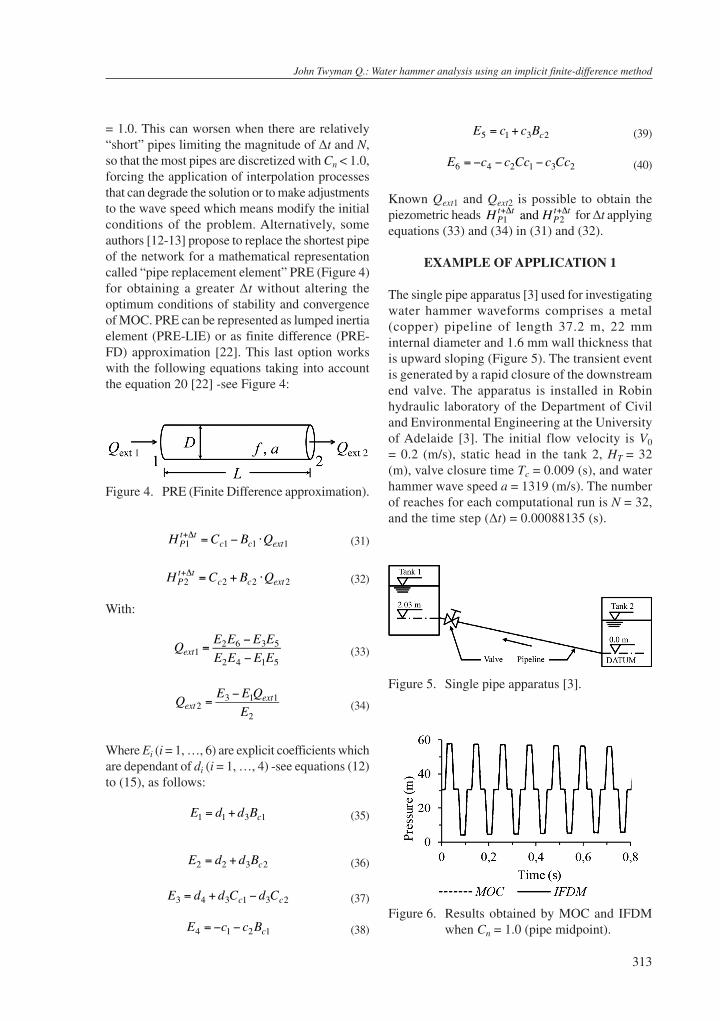
= 1.0. This can worsen when there are relatively “short” pipes limiting the magnitude of Δt and N, so that the most pipes are discretized with Cn < 1.0, forcing the application of interpolation processes that can degrade the solution or to make adjustments to the wave speed which means modify the initial conditions of the problem. Alternatively, some authors [12-13] propose to replace the shortest pipe of the network for a mathematical representation called “pipe replacement element” PRE (Figure 4) for obtaining a greater Δt without altering the optimum conditions of stability and convergence of MOC. PRE can be represented as lumped inertia element (PRE-LIE) or as finite difference (PRE-FD) approximation [22]. This last option works with the following equations taking into account the equation 20 [22] -see Figure 4:

Figure 4. PRE (Finite Difference approximation).

HP1t+Δt =Cc1 − Bc1 ⋅Qext1 (31)

HP2t+Δt =Cc2 + Bc2 ⋅Qext2 (32)

With:

Qext1 =E2E6 −E3E5E2E4 −E1E5

(33)

Qext2 =E3 −E1Qext1

E2(34)

Where Ei (i = 1, …, 6) are explicit coefficients which are dependant of di (i = 1, …, 4) -see equations (12) to (15), as follows:

E1 = d1+ d3Bc1 (35)

E2 = d2 + d3Bc2 (36)

E3 = d4 + d3Cc1 − d3Cc2 (37)

E4 = −c1 − c2Bc1 (38)

E5 = c1+ c3Bc2 (39)

E6 = −c4 − c2Cc1 − c3Cc2 (40)

Known Qext1 and Qext2 is possible to obtain the piezometric heads HP1

t+Δt and HP2t+Δt for Δt applying

equations (33) and (34) in (31) and (32).

EXAMPLE OF APPLICATION 1

The single pipe apparatus [3] used for investigating water hammer waveforms comprises a metal (copper) pipeline of length 37.2 m, 22 mm internal diameter and 1.6 mm wall thickness that is upward sloping (Figure 5). The transient event is generated by a rapid closure of the downstream end valve. The apparatus is installed in Robin hydraulic laboratory of the Department of Civil and Environmental Engineering at the University of Adelaide [3]. The initial flow velocity is V0 = 0.2 (m/s), static head in the tank 2, HT

= 32

(m), valve closure time Tc = 0.009 (s), and water hammer wave speed a = 1319 (m/s). The number of reaches for each computational run is N = 32, and the time step (Δt) = 0.00088135 (s).

Figure 5. Single pipe apparatus [3].

Figure 6. Results obtained by MOC and IFDM when Cn = 1.0 (pipe midpoint).


314

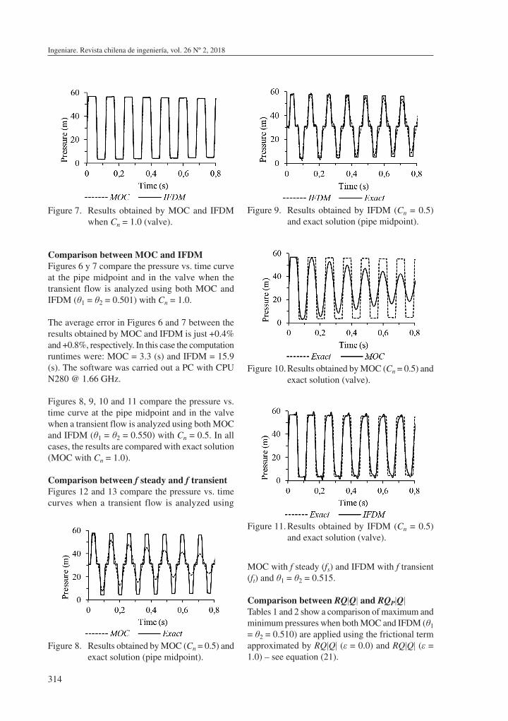
Comparison between MOC and IFDMFigures 6 y 7 compare the pressure vs. time curve at the pipe midpoint and in the valve when the transient flow is analyzed using both MOC and IFDM (θ1 = θ2 = 0.501) with Cn = 1.0.

The average error in Figures 6 and 7 between the results obtained by MOC and IFDM is just +0.4% and +0.8%, respectively. In this case the computation runtimes were: MOC = 3.3 (s) and IFDM = 15.9 (s). The software was carried out a PC with CPU N280 @ 1.66 GHz.

Figures 8, 9, 10 and 11 compare the pressure vs. time curve at the pipe midpoint and in the valve when a transient flow is analyzed using both MOC and IFDM (θ1 = θ2 = 0.550) with Cn = 0.5. In all cases, the results are compared with exact solution (MOC with Cn = 1.0).

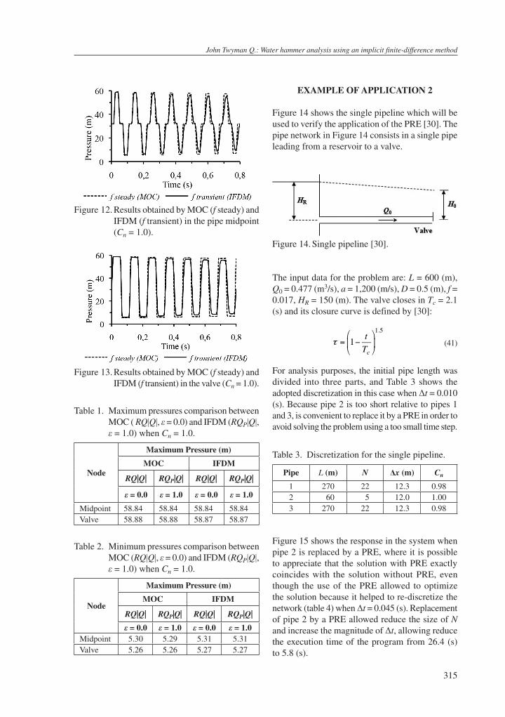
Comparison between f steady and f transientFigures 12 and 13 compare the pressure vs. time curves when a transient flow is analyzed using

Figure 7. Results obtained by MOC and IFDM when Cn = 1.0 (valve).

Figure 9. Results obtained by IFDM (Cn = 0.5) and exact solution (pipe midpoint).

Figure 10. Results obtained by MOC (Cn = 0.5) and exact solution (valve).

Figure 11. Results obtained by IFDM (Cn = 0.5) and exact solution (valve).

Figure 8. Results obtained by MOC (Cn = 0.5) and exact solution (pipe midpoint).

MOC with f steady (fs) and IFDM with f transient (ft) and θ1 = θ2 = 0.515.

Comparison between RQ|Q| and RQP|Q|Tables 1 and 2 show a comparison of maximum and minimum pressures when both MOC and IFDM (θ1 = θ2 = 0.510) are applied using the frictional term approximated by RQ|Q| (ε = 0.0) and RQ|Q| (ε = 1.0) – see equation (21).


315

Table 1. Maximum pressures comparison between MOC ( RQ|Q|, ε = 0.0) and IFDM (RQP|Q|, ε = 1.0) when Cn = 1.0.

Node

Maximum Pressure (m)

MOC IFDM

RQ|Q| RQP|Q| RQ|Q| RQP|Q|

ε = 0.0 ε = 1.0 ε = 0.0 ε = 1.0

Midpoint 58.84 58.84 58.84 58.84Valve 58.88 58.88 58.87 58.87

Table 2. Minimum pressures comparison between MOC (RQ|Q|, ε = 0.0) and IFDM (RQP|Q|, ε = 1.0) when Cn = 1.0.

Node

Maximum Pressure (m)

MOC IFDM

RQ|Q| RQP|Q| RQ|Q| RQP|Q|

ε = 0.0 ε = 1.0 ε = 0.0 ε = 1.0Midpoint 5.30 5.29 5.31 5.31Valve 5.26 5.26 5.27 5.27

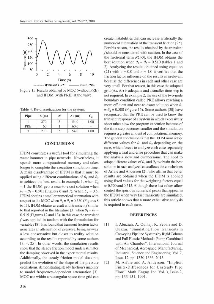
EXAMPLE OF APPLICATION 2

Figure 14 shows the single pipeline which will be used to verify the application of the PRE [30]. The pipe network in Figure 14 consists in a single pipe leading from a reservoir to a valve.

Figure 14. Single pipeline [30].

The input data for the problem are: L = 600 (m), Q0 = 0.477 (m3/s), a = 1,200 (m/s), D = 0.5 (m), f = 0.017, HR = 150 (m). The valve closes in Tc = 2.1 (s) and its closure curve is defined by [30]:

τ = 1− tTc

⎛

⎝⎜

⎞

⎠⎟1.5

(41)

For analysis purposes, the initial pipe length was divided into three parts, and Table 3 shows the adopted discretization in this case when Δt = 0.010 (s). Because pipe 2 is too short relative to pipes 1 and 3, is convenient to replace it by a PRE in order to avoid solving the problem using a too small time step.

Table 3. Discretization for the single pipeline.

Pipe L (m) N Δx (m) Cn

1 270 22 12.3 0.982 60 5 12.0 1.003 270 22 12.3 0.98

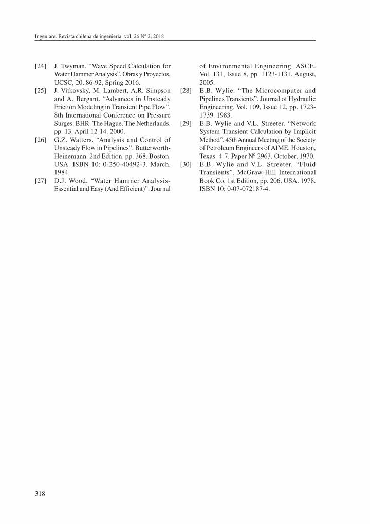
Figure 15 shows the response in the system when pipe 2 is replaced by a PRE, where it is possible to appreciate that the solution with PRE exactly coincides with the solution without PRE, even though the use of the PRE allowed to optimize the solution because it helped to re-discretize the network (table 4) when Δt = 0.045 (s). Replacement of pipe 2 by a PRE allowed reduce the size of N and increase the magnitude of Δt, allowing reduce the execution time of the program from 26.4 (s) to 5.8 (s).

Figure 12. Results obtained by MOC (f steady) and IFDM (f transient) in the pipe midpoint (Cn = 1.0).

Figure 13. Results obtained by MOC (f steady) and IFDM (f transient) in the valve (Cn = 1.0).


316

Figure 15. Results obtained by MOC (without PRE) and IFDM (with PRE) at the valve.

Table 4. Re-discretization for the system.

Pipe L (m) N Δx (m) Cn

1 270 5 54.0 1.00PRE 60 1 60.0 –

3 270 5 54.0 1.00

CONCLUSIONS

IFDM constitutes a useful tool for simulating the water hammer in pipe networks. Nevertheless, it spends more computational memory and takes longer to complete the execution simulation time. A main disadvantage of IFDM is that it must be applied using different combinations of θ1 and θ2 to achieve the best result. In example 1, when Cn = 1 the IFDM gets a near-to-exact solution when θ1 = θ2 = 0.501 (Figures 6 and 7). When Cn = 0.5, IFDM obtains a smaller numerical attenuation with respect to the MOC when θ1 = θ2 = 0.550 (Figures 8 to 11). IFDM obtains a result with transient f similar to that reported in the literature [3] when θ1 = θ2 = 0.515 (Figures 12 and 13). In this case the transient f was applied in tandem with the formulation for variable f [8]. It is found that transient friction factor generates an attenuation of pressure, being anyway a less conservative but closer to reality solution according to the results reported by some authors [3, 4, 25]. In other words, the simulation results show that the steady friction model underestimates the damping observed in the experimental results. Additionally, the steady friction model does not predict the evolution of the shape of the pressure oscillations, demonstrating steady friction’s inability to model frequency-dependent attenuation [3]. MOC use within a rectangular space-time grid can

create instabilities that can increase artificially the numerical attenuation of the transient friction [25]. For this reason, the results obtained by the transient f should be considered with caution. In the case of the frictional term RQ|Q|, the IFDM obtains the best solution when θ1 = θ2 = 0.510 (tables 1 and 2). Analyzing the results obtained using equation (21) with ε = 0.0 and ε = 1.0 it verifies that the friction factor influence on the results is irrelevant because the differences in each and other case are very small. For that reason, in this case the adopted grid (Δx, Δt) is adequate and a smaller time step is not required. In example 2, the use of the two-node boundary condition called PRE allows reaching a more efficient and near-to-exact solution when θ1 = θ2 = 0.500 (Figure 15). Some authors [30] have recognized that the PRE can be used to know the transient response of a system in which excessively short tubes slow the program execution because of the time step becomes smaller and the simulation requires a greater amount of computational memory. The general conclusion is that the IFDM must adopt different values for θ1 and θ2 depending on the case, which forces to analyze each case separately applying a trial and error procedure that can make the analysis slow and cumbersome. The need to adopt different values of θ1 and θ2 to obtain the best solution in each analyzed case allows the conclusions of Arfaie and Anderson [2], who affirm that better results are obtained when the IFDM is applied using fixed values for the weighting factors equal to 0.500 and 0.515. Although these last values allow control the spurious numerical peaks that appear in the IFDM when very fast transients are simulated, this article shows that a more exhaustive analysis is required in each case.

REFERENCES

[1] I. Abuziah, A. Oulhaj, K. Sebari and D. Ouazar. “Simulating Flow Transients in Conveying Pipeline Systems by Rigid Column and Full Elastic Methods: Pump Combined with Air Chamber”. International Journal of Mechanical, Aerospace, Manufacturing, Industrial Science and Engineering. Vol. 7, Issue 12, pp. 1330-1336. 2013.

[2] M. Arfaie and A. Anderson. “Implicit Finite-Differences for Unsteady Pipe Flow”. Math. Engng. Ind. Vol. 3, Issue 2, pp. 133-151. 1991.


317

[3] A. Bergant, A. Tijsseling, J. Vítkovský, D. Covas, A. Simpson and M. Lambert. “Further Investigation of Parameters Affecting Water Hammer Wave Attenuation, Shape and Timing Part 2: Case Studies”. Journal of Hydraulic Research. Vol. 46, Issue 3, pp. 382-391. July, 2008.

[4] B. Brunone, B.W. Karney, M. Mecarelli and M. Ferrante. “Velocity Profiles and Unsteady Pipe Friction in Transient Flow”. Journal of Water Resources Planning and Management. Vol. 126, Issue 4, pp. 236-244. July/August, 2000.

[5] M.H. Chaudhry “Applied Hydraulic Transients”. Van Nostrand Reinhold. 1st Edition. New York. USA, pp. 266. 1979. ISBN 10: 0-442-21517-7.

[6] M.H. Chaudhry “Numerical Solution of Transient-Flow Equations”. Proc. Speciality Conf. Hydraulics Division, ASCE Jackson, MS, pp. 633-656. August, 1982.

[7] M.H. Chaudhry and M.Y. Hussaini. “Second-Order Accurate Explicit Finite-Difference Schemes for Waterhammer Analysis”. Journal of Fluids Engineering. Vol. 107, pp. 523-529. April, 1985.

[8] J.J.J. Chen and A.D. Ackland. “Correlation of Laminar, Transitional and Turbulent Flow Friction Factor”. Proc. Instn. Civ. Engrs. Part 2, 89. 573-576. December. 1991.

[9] M.S. Ghidaoui, M. Zhao, D.A. McInnis, D.H. Axworthy. “A Review of Water Hammer Theory and Practice”, Applied Mechanics Review, ASME. Vol. 58, pp. 49-76. January, 2005.

[10] D.E. Goldberg and E.B. Wylie. “Characteristics Method using Time-Line Interpolations”. Journal of Hydraulic Engineering. Vol. 109, Issue 5, pp. 670-683. May, 1983.

[11] M.B. Holloway and M.H. Chaudhry. “Stability and Accuracy of Waterhammer Analysis”. Adv. Water Resources. Vol. 8, pp. 121-128. 1985.

[12] B.W. Karney. “Analysis of Fluids Transients in Large Distribution Networks”. PhD Thesis, University of British Columbia, Canada, pp. 146. 1984.

[13] B.W. Karney and D. McInnis. “Efficient Calculation of Transient Flow in Simple Pipe Networks”. Journal of Hydraulic Engineering. ASCE. Vol. 118, Issue 7, pp. 1014-1030. 1992.

[14] Y. Kim. “Advanced Numerical and Experimental Transient Modeling of Water and Gas Pipeline Flows Incorporating Distributed and Local Effects”. School of Civil, Environmental and Mining Engineering. PhD Thesis. The University of Adelaide. Australia, pp. 146. 2008.

[15] A. Malekpour, B.W. Karney. “Spurious Numerical Oscillations in the Preissmann Slot Method: Origin and Suppression”. Journal of Hydraulic Engineering. ASCE, pp. 12. 2015.

[16] R.O. Salgado. “Revisión de los Métodos Numéricos para el Análisis del Escurrimiento Impermanente en Redes de Tuberías a Presión”. XV Congreso Latinoamericano de Hidráulica, AIHR, AIIH, IAHR. Cartagena, Colombia. 1992.

[17] R.O. Salgado, J. Zenteno, C. Twyman and J. Twyman. “A Hybrid Characteristics-Finite Difference Method for Unsteady Flow in Pipe Networks”. International Conference on Integrated Computer Applications for Water Supply and Distribution. De Montfort University. Leicester. UK, pp. 139-149. 1993.

[18] H.M.V. Samani and A. Khayatzadeh. “Transient Flow in Pipe Networks”. Journal of Hydraulic Research. Vol. 40, Issue 5, pp. 637-644. May, 2001.

[19] M. Sepehran and M.A. Badri. “Water Hammer Simulation by Implicit Finite Difference Scheme Using Non-Symmetrical Staggered Grid”. Recent Advances in Fluid Mechanics, Heat & Mass Transfer and Biology, pp. 47-52. ISBN: 978-1-61804-065-7.

[20] V.L. Streeter and C. Lai. “Water-Hammer Analysis Including Fluid Friction”. Journal of the Hydraulics Division. ASCE. Vol. 88. Paper HY3. 79-111. 1962.

[21] V.L. Streeter, E.B. Wylie. “Waterhammer and Surge Control”. Annual Reviews Fluid Mechanics, pp. 57-73. 1973.

[22] J. Twyman. “Decoupled Hybrid Methods for Unsteady Flow Analysis in Pipe Networks”. Ed. La Cáfila. 1st Edition. Valparaíso, Chile, pp. 185. 2004. ISBN 10: 956-8142-17-7.

[23] J. Twyman. “Golpe de Ariete en una Red de Distribución de Agua”. Anales del XXVII Congreso Latinoamericano de Hidráulica (IAHR Spain Water & IWHR China). Lima, Perú, pp. 10. Septiembre 2016.


318

[24] J. Twyman. “Wave Speed Calculation for Water Hammer Analysis”. Obras y Proyectos, UCSC, 20, 86-92, Spring 2016.

[25] J. Vítkovský, M. Lambert, A.R. Simpson and A. Bergant. “Advances in Unsteady Friction Modeling in Transient Pipe Flow”. 8th International Conference on Pressure Surges. BHR. The Hague. The Netherlands. pp. 13. April 12-14. 2000.

[26] G.Z. Watters. “Analysis and Control of Unsteady Flow in Pipelines”. Butterworth-Heinemann. 2nd Edition. pp. 368. Boston. USA. ISBN 10: 0-250-40492-3. March, 1984.

[27] D.J. Wood. “Water Hammer Analysis-Essential and Easy (And Efficient)”. Journal

of Environmental Engineering. ASCE. Vol. 131, Issue 8, pp. 1123-1131. August, 2005.

[28] E.B. Wylie. “The Microcomputer and Pipelines Transients”. Journal of Hydraulic Engineering. Vol. 109, Issue 12, pp. 1723-1739. 1983.

[29] E.B. Wylie and V.L. Streeter. “Network System Transient Calculation by Implicit Method”. 45th Annual Meeting of the Society of Petroleum Engineers of AIME. Houston, Texas. 4-7. Paper Nº 2963. October, 1970.

[30] E.B. Wylie and V.L. Streeter. “Fluid Transients”. McGraw-Hill International Book Co. 1st Edition, pp. 206. USA. 1978. ISBN 10: 0-07-072187-4.

water hammer analysis using an implicit finite-difference ... · water hammer analysis using an...

Documents