WATER ENTRY OF A BODY WHICH MOVES INMORE THAN SIX DEGREES OF FREEDOM.

Y.-M. SCOLAN1 AND A. A. KOROBKIN2

1ENSTA Bretagne, LBMS, Brest, France2School of Mathematics, University of East Anglia, Norwich, NR4 7TJ, UKEmail address for correspondence: yves-marie.scolan@ensta-bretagne.fr

Abstract

The water entry of a three-dimensional smooth body into initially calm water is examined.

The body can move freely in its six degrees of freedom and may also change its shape over

time. During the early stage of penetration, the shape of the body is approximated by a surface

of double curvature and the radii of curvature may vary over time. Hydrodynamic loads are

calculated by the Wagner theory. It is shown that the water entry problem with arbitrary

kinematics of the body motion, can be reduced to the vertical entry problem with a modified

vertical displacement of the body and an elliptic region of contact between the liquid and the

body surface. Low pressure occurence is determined; this occurence can precede the appearance

of cavitation effects. Hydrodynamic forces are analysed for a rigid ellipsoid entering the water

with three degrees of freedom. Experimental results with an oblique impact of elliptic paraboloid

confirm the theoretical findings. The theoretical developments are detailed in the present paper,

while an application of the model is described in supplementary materials.

keywords: Water impact, three-dimensional flow, free body motion, hydrodynamic loads.

1 Introduction

We consider a three-dimensional object with a smooth surface, such as the bow part of a ship hullor the fuselage of an aircraft, approaching the water surface after lifting off or arriving from theatmosphere and penetrating the liquid free surface. The body motion can be computed only bynumerical means by taking into account the large displacements of the body, the cavity forma-tion behind the body and the viscous forces acting on the body surface. This problem was stud-ied by [Kleefsman et al.(2005)], [Maruzewski et al.(2010)], [Tassin et al.(2013)], [ Yang & Qiu(2012)]among others. The early stage of water entry, when the wetted surface is in rapid expansion, is diffi-cult to capture numerically but this is the stage during which the hydrodynamic loads acting on thebody are very high and may affect the body motions even for longer times.

We focus on the initial stage of the three-dimensional motion of a free body just after the timeinstant, t = 0, at which the body touches the water surface at a single point.We consider bodieswhose dimensions are of the order of few metres, such as the fuselage of an aircraft or the bow partof a ship hull. For the water entry of such shapes the following assumptions are usually made : i) theviscous effects are neglected since neither a boundary layer nor a separated flow has time enough todevelop, ii) the surface tension effects are not taken into account since the local curvature of the freesurface is very small (except at the jet root), and iii) the acceleration of the fluid particles exceedsthe acceleration of gravity. Those are the reasons for which neither Reynolds nor Froude and Webernumbers are included in the present problem.

In the present analysis, the liquid is assumed to be incompressible and inviscid. The generatedflow is irrotational and three-dimensional. Initially, t = 0, the water surface is flat and horizontal.The body surface in the contact region is approximated by a double curvature surface with two radiiof curvature, Rx and Ry, which are not necessarily equal and may depend on time t.

1

X

Y

Z

O

Z

X

Y

D(t)

physicaldomain

linearizeddomain

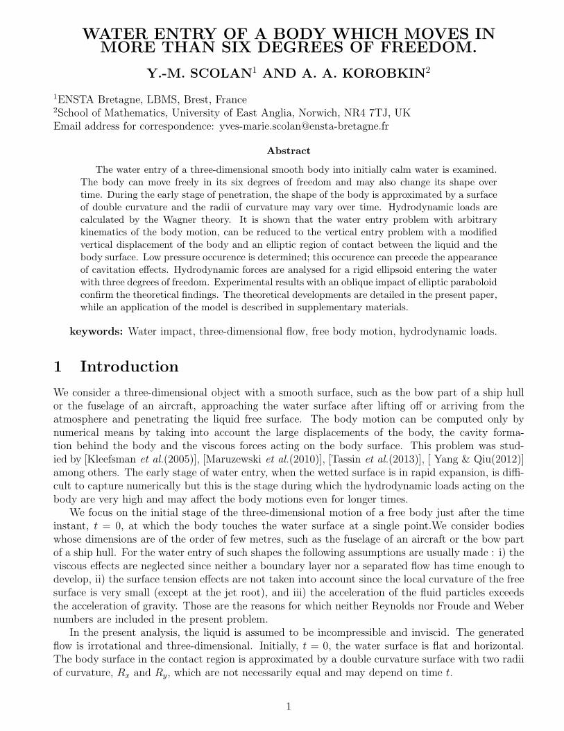
Figure 1: Sketch of a three dimensional body entering an initially flat free surface. The translationaland rotational motions (thick arrows) are described in an earth fixed coordinate system. In thelinearised domain, D(t) is the instantaneous expanding wetted surface. This is the projection of theactual wetted surface on the horizontal plane (x, y). The contact line is the intersection line betweenthe moving body surface and the deformed free surface in both physical and linearized domain.

Under the assumption of large curvature radii compared to the penetration depth, the resultingboundary-value problem is known as the Wagner entry problem (see [Wagner(1932)]) or ”flat-diskapproximation” or Wagner’s approach. This three-dimensional problem was studied in the pastfor the standard case of the vertical entry of an elliptic paraboloid (see [Scolan & Korobkin(2001),Korobkin(2002), Scolan & Korobkin(2003), Korobkin & Scolan(2006)]). Note that the Wagner the-ory assumes small deadrise angles and the wetted area, which expands in all directions over time.For more complex body motions, the oblique impact of an axisymmetric body was studied in[Moore et al.(2012)] and the oblique impact of an elliptic paraboloid in [Scolan & Korobkin(2012)].The present paper aims at generalizing the entry of a smooth three-dimensional body that moves inall possible DoF and changes its shape over time as well. We are unaware of results by others deal-ing with such complex motions of the body entering water and the corresponding three-dimensionalflows. It is shown in the present paper that angular motions of a body change significantly thehydrodynamic loads and their distributions over the wetted part of the body surface. The pressuredistribution is carefully analysed in section 5, the zones of negative loads are identified, and theduration of the Wagner stage is examined.

The physical formulation of the entry problem within the Wagner approach is illustrated in Figure(1). The jet flow originated at the periphery of the wetted part of the body surface is not shown inthis Figure. The water entry problem for an arbitrary smooth body is formulated in terms of the

2

displacement potential φ(x, y, z, t) (see [Korobkin(1985), Howison et al.(1991)])

∇2φ = 0 (z < 0),φ = 0 (z = 0, (x, y) /∈ D(t)),φ,z = f(x, y, t) (z = 0, (x, y) ∈ D(t)),φ → 0 (x2 + y2 + z2 → ∞),φ ∈ C2(z < 0) ∩ C1(z ≤ 0) .

(1)

Here the lower half-plane z < 0 corresponds to the flow domain, D(t) is the contact region between theentering body and the liquid, the rest of the boundary, z = 0, (x, y) /∈ D(t), corresponds to the liquidfree surface. The position of the entering body surface is described by the equation z = f(x, y, t).In this paper, the function f(x, y, t) includes the six degrees of freedom of the rigid body motionsand the deformations of the body surface expressed in an earth fixed coordinate system. The lastcondition in (1) implies that the displacement potential φ is a smooth function in the flow region,and is continuous together with its first derivatives φ,x, φ,y and φ,z up to the boundary including theboundary (see [Korobkin & Pukhnachov(1988)]). The latter condition is equivalent to the Wagnercondition (see [Wagner(1932)]) and serves to determine the shape and position of the contact regionD(t). Note that the time t is a parameter in this formulation. The problem can be solved at any timeinstant independently. The derivatives φ,x, φ,y and φ,z provide the displacements of liquid particlesin the corresponding directions.

The function f(x, y, t) from (1) is determined in §2 for the given motions of a rigid body. Thedisplacement potential φ(x, y, 0, t) in the contact region D(t) and the shape of this region are de-termined in §3. Hydrodynamic forces and moments acting on the body are calculated in §4. Thehydrodynamic pressure distribution is analysed in §5. In §6, we consider the problem of a rigidellipsoid entering water surface at an angle of attack. The obtained results are summarised andconclusions are drawn in §7.

2 Shape function of a body during its impact on the water

surface

To determine the function f(x, y, t) in (1), we consider the equations describing the position of thesurface of a moving body by taking into account a possible variation of the body shape over time.Let the surface of the body be described by the equation z1 = F (x1, y1, t) in the coordinate systemmoving together with the body and such that the global x, y, z and local x1, y1, z1 coordinates coincideat the impact instant t = 0. Here F (0, 0, t) = 0, F,x1

(0, 0, t) = 0, F,y1(0, 0, t) = 0, and F (x1, y1, t) > 0,

where |x1| > 0, |y1| > 0 are small. The body surface, z1 = F (x1, y1, t), is hence approximated closeto the origin by the Taylor series

z1 =x2

1

2Rx(t)+

y21

2Ry(t)+ O(r4

1/R3), (2)

where r21 = x2

1 + y21 and R is an averaged curvature radius. We suppose that Ry(t) ≥ Rx(t) and

introduce ǫ =√

1 − Rx(t)/Ry(t) as the eccentricity of the horizontal, z1 = const, sections of theelliptic paraboloid (2).

The body displacements in x−, y− and z−directions are given by the functions xb(t), yb(t)and −h(t) respectively. The body also rotates with an angle αx(t) around the x1-axis (roll angle),αy(t) around the y1-axis (pitch angle), αz(t) around the z1-axis (yaw angle). We assume that thedisplacements xb(t), yb(t), h(t) and the angles αx(t), αy(t), αz(t) are small and equal to zero at t = 0.The penetration depth h(t) is chosen here to characterise the initial stage during which h(t)/Rx(t) ≪1. The orders of other displacements and angles will be specified below.

3

For small angles of rotation the global and local coordinates are related by the following equations

x = x1 + xb(t) − y1αz(t) − z1αy(t), (3)

y = y1 + yb(t) + x1αz(t) − z1αx(t), (4)

z = z1 − h(t) + x1αy(t) + y1αx(t). (5)

The linear size of the wetted area is estimated by neglecting all motions except the vertical oneand by neglecting the free surface elevation. Within this rough approximation, the wetted area isenclosed by the intersection line between the entering body z = x2/(2Rx(t)) + y2/(2Ry(t)) − h(t)

and the plane z = 0. Therefore, x and y in the wetted area are of the order of√

h(t)Rx(t) for smallh(t)/Rx(t). All terms in equations (3)-(5) are of the same order during the initial stage if xb(t) andyb(t) are of the order of

√

h(t)Rx(t), and the angles αx(t), αy(t) = O(√

h(t)/Rx(t)), αz(t) = O(1)as h(t)/Rx(t) ≪ 1. Note that any yaw angles are allowed but we assume αz(t) ≪ 1 in the nextdevelopments, keeping in mind that the duration of the initial stage is small and the yaw angle, asother angles cannot vary significantly during this short period. With these orders of the motionsall terms in (5) are of the same order. In (4), all terms are of order of O(

√

h(t)Rx(t)) except the

last term which is of a higher order, O(√

h3(t)/Rx(t)), and can be neglected in the leading order.A similar analysis applied to (3) finally provides that relations (3)-(5) can be approximated in theleading order by

x = x1 + xb(t), y = y1 + yb(t), z = z1 − h(t) + x1αy(t) + y1αx(t). (6)

Substituting (6) in (2) and rearranging the terms, we obtain

z =(x − X(t))2

2Rx(t)+

(y − Y (t))2

2Ry(t)− Z(t), (7)

whereX(t) = xb(t) − Rx(t)αy(t), Y (t) = yb(t) − Ry(t)αx(t), (8)

Z(t) = h(t) +1

2[Ry(t)α

2x(t) + Rx(t)α

2y(t)]. (9)

The right-hand side in (7) provides the function f(x, y, t) in the formulation (1). Note that thehorizontal displacements of the body, xb(t) and yb(t), are allowed to be much greater than thevertical displacement h(t).

3 Displacement potential in the contact region

The expression of the shape function f(x, y, t) following from equation (9) makes it possible tointroduce the self-similar variables λ, µ, ν as in [Korobkin(2002)]

x = X(t) + B(t)λ, y = Y (t) + B(t)µ, z = B(t)ν, B(t) =√

2Rx(t)Z(t), (10)

and the new potential Φ(λ, µ, ν) by

φ = Z(t)B(t)Φ(λ, µ, ν). (11)

The boundary-value problem with respect to the new unknown potential Φ follows from (1)

∇2Φ = 0 (ν < 0),Φ = 0 (ν = 0, (λ, µ) /∈ Dǫ),Φ,ν = λ2 + (1 − ǫ2)µ2 − 1 (ν = 0, (λ, µ) /∈ Dǫ),Φ → 0 (λ2 + µ2 + ν2 → ∞),Φ ∈ C2(ν < 0) ∩ C1(ν ≤ 0).

(12)

4

Here Dǫ is the contact region in the stretched variables. Its shape depends on the only parameterǫ =

√

1 − Rx(t)/Ry(t). The problem (12) is the same as that for an elliptic paraboloid enteringthe liquid vertically at constant speed. The solution of the latter problem was well investigated by[Scolan & Korobkin(2001), Korobkin(2002), Scolan & Korobkin(2003), Korobkin(2005)] in the past.It was found that the contact region Dǫ is the ellipse

λ2

a2+

µ2

b2≤ 1, (13)

where a =√

1 − e2b, b =√

3/(2 − e2 − ǫ2) and e(ǫ) is the eccentricity of the contact region definedby the equation

ǫ2 =2(e4 − e2 + 1)E(e)/K(e) − (1 − e2)(2 − e2)

(1 + e2)E(e)/K(e) + e2 − 1, (14)

K(e) and E(e) are the complete elliptic integrals of the first and second kind as defined in [Gradshteyn & RyzhikThe displacement potential Φ(λ, µ, 0) in the contact region is given by [Korobkin(2002)] in the form

Φ(λ, µ, 0) = − 2a

3E(e)

(

1 − λ2

a2− µ2

b2

)3

2

. (15)

Note that the displacement potential (15) in the stretched coordinates system does not depend onany motions but only on the eccentricity of the body sections. This eccentricity can be a function oftime.

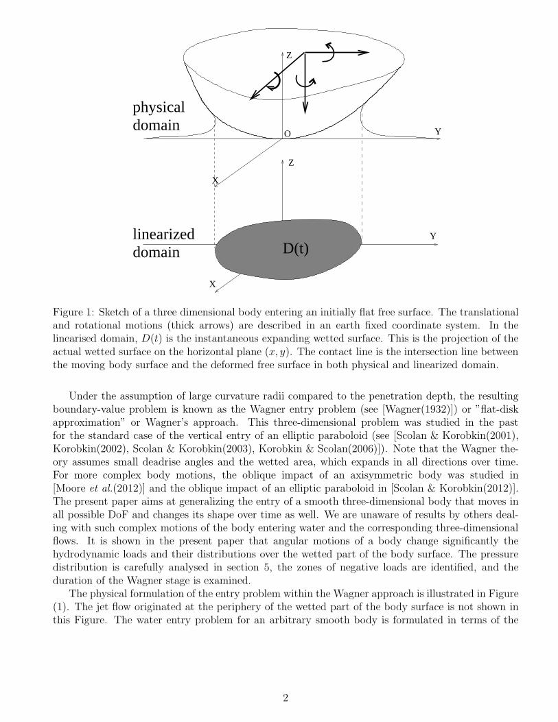
The comparison between theoretical and experimental results are illustrated in Figures (2) and(3). We consider the oblique entry of an elliptic paraboloid defined by the constant curvature radiiRx = 0.75m and Ry = 2m. The kinematics of the moving (undeformable) body reduce to twotranslational motions in the plane (y, z). The y-horizontal and vertical velocities are yb = 0.59m/sand h = 0.79m/s respectively. The expansion of the wetted surface is computed and compared tothe observations made during an experimental programme at BGO First (La Seyne/Mer, France) in2011. This programme is described in [Scolan(2012)]. A submerged camera is placed on the basinfloor below the impact point. It records along a vertical axis upwards at a frequency of 200 framesper second. In Figure (2) the periphery of the wetted surface at different time instants is markedby a thick white line. Indeed this line is elliptic and it is not affected by the horizontal motion.The results are collected in figure (3). Since the velocities are constant, it is expected that the

lengths of the wetted surface increase as√

t, hence the quantities aB/√

h and bB/√

h are plotted interms of

√t. The variation is therefore linear. The agreement is satisfactory since the error between

experiments and theory is within 10%, even at the initial stage where it is more difficult to detectthe contact line accurately. The absolute error ∆a of measurement is approximately one third thesize of the cell grid (0.05m) yielding the highest relative error of 20%. More results are availablein [Scolan & Korobkin(2012)]. In particular it is observed that the theory slightly overpredicts theexperimental data regarding the size of the wetted surface.

4 Hydrodynamic loads and equations of the body motions

Taking into account that the hydrodynamic pressure p, the velocity potential ϕ and the displacementpotentail φ as well, are zero on the free surface and at infinity, the expressions of the force ~F andmoment ~M can reduce to

~F (t) =d

dt

∫ ∫

D(t)

ρϕ~ndS, ~M(t) =d

dt

∫ ∫

D(t)

ρϕ(~r × ~n)dS, (16)

5

Figure 2: Snapshots of the expanding wetted surface for an oblique entry of elliptic paraboloid definedby Rx = 0.75m, Ry = 2m. The experimental set-up is described in [Scolan(2012)]. The constantvertical velocity and y-horizontal velocity are h = 0.79m/s and yb = 0.59m/s respectively. There areno rotations in the experiments. The camera records at 200Hz. The periphery of the wetted area ofthe body surface at different time instants is marked by a thick white line.

6

0

0.1

0.2

0.3

0.4

0.5

0.6

0 0.05 0.1 0.15 0.2 0.25√

time(s)

aB(t)/√

h

bB(t)/√

htheoretical

experimental

b

b

b

b

bb

b

b

b

b

b

b

b

b

b

b

b

b

b

b

b

Figure 3: Time variations of the major and minor semi-axes of the elliptic wetted surface, respectively

bB(t) and aB(t), divided by√

h. Comparison of experimental data (marks) and theoretical results(solid lines). The vertical velocity and y-horizontal velocity are h = 0.79m/s and yb = 0.59m/srespectively.

as shown in [Kochin et al.(1964)] for a body moving in unbounded fluid (see pp 394-397). Here ρ

is the density of the liquid. The hydrodynamic moment ~M1(t) with respect to the point of the firstcontact on the body surface, ~rb(t) = (xb, yb,−h), is calculated as

~M1(t) = ~M(t) − ~rb(t) × ~F (t), (17)

If the position of the entering body is given by the equation z = f(x, y, t) as in (1), then

~r = (x, y, f(x, y, t)), ~ndS = (f,x, f,y,−1)dxdy. (18)

The shape function f(x, y, t) is given by (7) and the displacement potential φ by (11) and (15). Itshould be noted that ff,x, ff,y = O(h

√

h/Rx) and x, y = O(√

hRx). Therefore, the terms ff,x andff,y can be neglected with the relative accuracy O(h/Rx). The vertical component of the moment issmaller than two other components and the hydrodynamic loads do not depend on the small yaw angleαz(t). Therefore, the yaw motion can be computed by integration of the corresponding equation,in which the moment is independent of this angle, after other motions have been determined. Theequation for the yaw angle is not considered in the following.

Evaluating the integrals in (16), we obtain

Fx(t) = − d

dt

(

ρA(t)

Rx(t)

dX

dt

)

, Fy(t) = − d

dt

(

ρA(t)

Ry(t)

dY

dt

)

, Fz(t) =d2

dt2

(

ρA(t))

, (19)

Mx(t) =d2

dt2

(

ρA(t)Y (t))

, My(t) = − d2

dt2

(

ρA(t)X(t))

, (20)

A(t) = −∫ ∫

D(t)

φ(x, y, 0, t)dxdy = N(ǫ)Z5

2 (t)R3

2

x , N(ǫ) =8√

2πa2b

15E(e). (21)

Note that ǫ in (21) can be a function of time for varying radii of the body curvature. It is importantto note that Fz(t) is independent of the body displacements xb(t) and yb(t) in horizontal directions.However, the force and the moments are strongly dependent on the angles of the body rotations.

7

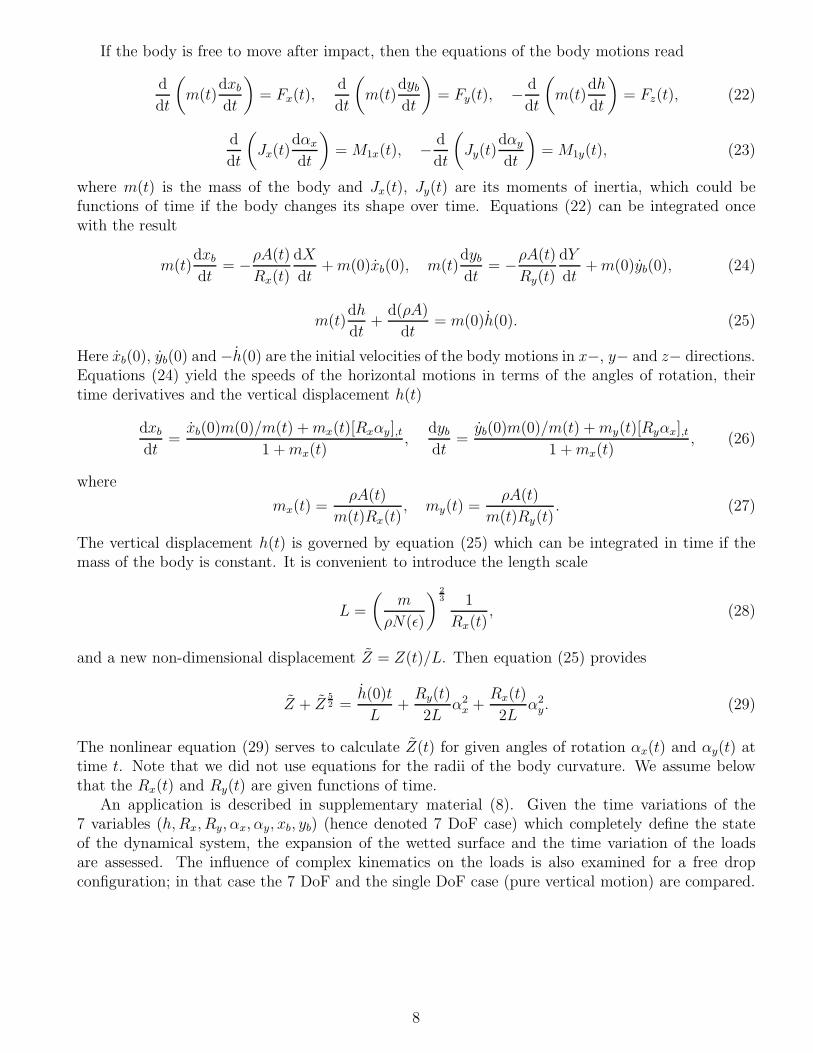
If the body is free to move after impact, then the equations of the body motions read

d

dt

(

m(t)dxb

dt

)

= Fx(t),d

dt

(

m(t)dyb

dt

)

= Fy(t), − d

dt

(

m(t)dh

dt

)

= Fz(t), (22)

d

dt

(

Jx(t)dαx

dt

)

= M1x(t), − d

dt

(

Jy(t)dαy

dt

)

= M1y(t), (23)

where m(t) is the mass of the body and Jx(t), Jy(t) are its moments of inertia, which could befunctions of time if the body changes its shape over time. Equations (22) can be integrated oncewith the result

m(t)dxb

dt= −ρA(t)

Rx(t)

dX

dt+ m(0)xb(0), m(t)

dyb

dt= −ρA(t)

Ry(t)

dY

dt+ m(0)yb(0), (24)

m(t)dh

dt+

d(ρA)

dt= m(0)h(0). (25)

Here xb(0), yb(0) and −h(0) are the initial velocities of the body motions in x−, y− and z− directions.Equations (24) yield the speeds of the horizontal motions in terms of the angles of rotation, theirtime derivatives and the vertical displacement h(t)

dxb

dt=

xb(0)m(0)/m(t) + mx(t)[Rxαy],t1 + mx(t)

,dyb

dt=

yb(0)m(0)/m(t) + my(t)[Ryαx],t1 + mx(t)

, (26)

where

mx(t) =ρA(t)

m(t)Rx(t), my(t) =

ρA(t)

m(t)Ry(t). (27)

The vertical displacement h(t) is governed by equation (25) which can be integrated in time if themass of the body is constant. It is convenient to introduce the length scale

L =

(

m

ρN(ǫ)

)2

3 1

Rx(t), (28)

and a new non-dimensional displacement Z = Z(t)/L. Then equation (25) provides

Z + Z5

2 =h(0)t

L+

Ry(t)

2Lα2

x +Rx(t)

2Lα2

y. (29)

The nonlinear equation (29) serves to calculate Z(t) for given angles of rotation αx(t) and αy(t) attime t. Note that we did not use equations for the radii of the body curvature. We assume belowthat the Rx(t) and Ry(t) are given functions of time.

An application is described in supplementary material (8). Given the time variations of the7 variables (h, Rx, Ry, αx, αy, xb, yb) (hence denoted 7 DoF case) which completely define the stateof the dynamical system, the expansion of the wetted surface and the time variation of the loadsare assessed. The influence of complex kinematics on the loads is also examined for a free dropconfiguration; in that case the 7 DoF and the single DoF case (pure vertical motion) are compared.

8

5 Pressure distribution

The pressure follows from the linearised Bernoulli equation p = −ρϕ,t = −ρφ,t2 , where φ(x, y, 0, t) inthe wetted area is given by (10), (11) and (15). If we note φ = −G3/2(x, y, t), then G appears as apolynomial of order two with respect to x and y and we can express G as

G(x, y, t) =

i+j≤2∑

i,j=0

βij(t)xiyj, (30)

where all (non zero) coefficients βij only depend on time. Then the pressure can be expressed as

p =3ρ

4√

G

(

2GG + G2)

, (31)

where overdot stands for time derivative and the expression 2GG + G2 is a polynomial of order 4 inx and y.

We first examine the behaviour of the pressure close to the contact line, where G(x, y, t) vanishesand the pressure is approximated by

p(x, y, 0, t) ≈ 3

4ρ

C3/2

√

1 − λ2/a2 − µ2/b2

(

∂

∂t

(

λ2

a2+

µ2

b2

))2

. (32)

The time derivative in (32) is calculated for fixed x and y by taking into account the relations (10)between x, y and λ, µ. As also noted by [Moore et al.(2012)], this time derivative is proportionalto the normal velocity of expansion of the wetted surface and the first time instant t⋆, when thisderivative is zero, provides the duration of the Wagner stage of impact. To find t⋆ and the place onthe expanding contact line, where the derivative is zero at t⋆, we search the minimum of the timederivative in (32). After some manipulations, and assuming that the ratio Rx(t)/Ry(t) does notdepend on time, it is shown that t⋆ is obtained from

a2B2(t⋆) = X2(t⋆) + k2Y 2(t⋆). (33)

Equation (33) provides the duration of the Wagner stage t⋆ for a body whose aspect ratio kγ =√

Rx/Ry is constant and which moves with 5 DoF. Note that the yaw motion can be approximatelyneglected during the early stage of impact. Under the same assumptions, it is also shown that thepressure vanishes in the direction of the translational motion. The calculations are more complicatedfor a general case where kγ is a function of time.

We are concerned in the following with the zones of negative pressure in the contact region. Thesezones are bounded by the lines p(x, y, 0, t) = 0 which are defined by the equation G2 + 2GG = 0 asfollows from (31). In the latter equation, the first term is positive and G(x, y, t) ≥ 0 in the contactregion. Therefore, the negative pressure zone may exist only if G(x, y, t) ≤ 0. Then it would be ofinterest to determine the roots of the polynomial G2 + 2GG. In practice it is not an easy task tofind the lines p = 0. On the other hand, provided that the time variations of (h, Rx, Ry, αx, αy, xb, yb)are given, the numerical computations of the coefficients βij and their first and second derivativesin time are rather staightforward. For example, a finite difference scheme is expected to be accurateenough to compute βij and βij if the time variations of (h, Rx, Ry, αx, αy, xb, yb) are regular.

The pressure distribution on the wetted surface is studied below for a rigid three-dimensionalbody with constant radii of curvature Rx and Ry. In this case, the identity holds: 2ZB = ZB atany time, and G calculated from (30) does not contain polynomials of x and y greater than 1. Byintroducing the change of variables between coordinates systems (λ, µ), and (ξ, η) as follows

ξ(x, y, t) =

√2

a

(

a2B

2+ λX + k2µY

)

, η(x, y, t) =1

b

(

µX − λY)

, (34)

9

we can re-arrange 2GG + G2 in equation (31), so that

4p√

G

3ρH2= 2Z

(

1 − λ2

a2− µ2

b2

)

G(2) +4Z2

a2B2

(

a2B2

2− X2 − k2Y 2 + ξ2 + η2

)

. (35)

with

G(2) =

(

a√

8Rx

3E

)2/3(

Z +2Z

B

(

λX

a2+

µY

b2

))

, (36)

We can conclude that the second term in (35) is positive in the contact region D(t) as long as

T (t) =a2B2

2− X2 − k2Y 2 > 0. (37)

The criterion (37) is quite in line with the results of [Moore et al.(2012)] who dealt with the obliqueentry of an elliptic paraboloid as well. As soon as the left hand side of equation (37) changes itssign, and provided the body motion is such that G(2) = 0, the pressure becomes negative in a regionwhich is circular in variables (ξ, η) and starts to increase from ξ = 0 and η = 0. The location of thefirst point (xo, yo) in the contact region where p ≤ 0, and the time instant of its appearance to aredefined by ξ(xo, yo, to) = 0 and η(xo, yo, to) = 0, with

xo = X − Xa2BB

2(X2 + k2Y 2), yo = Y − Y a2BB

2(X2 + k2Y 2), (38)

where all quantities are evaluated at time to. Once it happens, the wetted surface where the pressureis negative increases monotonically. The corresponding surface is a circle in the coordinate system(ξ, η). In the coordinate system (x, y), that area is constructed parametrically by inverting the linearsystem (34) with ξ = rT (t) cos γ and η = rT (t) sin γ, where r ∈ [0, 1] and γ ∈ [0, 2π].

As an example, we restrict the body kinematics to translational motions in the plane (y, z) with

X = 0. By introducing the non-dimensional measure of time τ = YbB

, the instant at which the

pressure first vanishes in the contact region corresponds to τ = 1√2

as it follows from equation (37).The expanding elliptic area of negative pressure is enclosed by the curve

x2

a2B2+ 2

(y − Y + bB2τ

)2

b2B2= 1 − 1

2τ 2. (39)

The ellipse (39) is centered at a point xe = 0 and ye = Y − bB2τ

, in the downstream part of the wetted

surface with respect to the y translational motion. The aspect ratio of this ellipse is√

2k and can begreater than 1 if Rx/Ry > 0.42. Note that the aspect ratio of the contact region (13) is equal to k.The time t⋆ at which the negative pressure zone (39) approaches the contact line (13) corresponds toτ = 1 i.e. when the translational velocity Y becomes equal to the velocity of expansion of the wettedsurface bB. The corresponding point of intersection is xi = 0 and yi = Y −bB. The negative pressurearea hence extends over half the wetted surface, downstream. At the point of intersection, the radiiof curvature (in the horizontal plane) of the two curves, the contact line and the zero pressure line(equation 39), are identical bBk2. Therefore the two curves do not intersect elsewhere than at point(xi, yi).

In supplementary material (8), the evolution of the negative pressure zone is assessed for a moregeneral case. It is shown that the negative pressure surface may expand much faster than the wettedsurface itself.

10

6 Oblique impact of an ellipsoid on the flat free surface

This section is motivated by the problem of aircraft landing on the water surface. The fuselage ofan aircraft is an elongated structure and hydrodynamic loads acting on it during landing can bedescribed by the strip theory [Tassin et al.(2013)]. By ”strip theory” we mean a way to constructa three-dimensional flow solution over an elongated body by computing successive twodimensionalsolutions in cross sections perpendicular to the direction of the maximum elongation of a body.However, at the very beginning of the landing, the contact region of the fuselage is not elongatedand the three-dimensional impact theory should be used to describe the loads during this stage.

As an illustration we consider the oblique impact of the ellipsoid

x2

a2+

y2

b2+

z2

c2= 1 (40)

on an initially flat water surface z = 0. In equation (40), x, y and z are local coordinates withthe origin at the centre of the ellipsoid, and a, b and c are the corresponding semi-axis. Initially,the ellipsoid is above the flat free surface, inclined at an angle α0 and touches the free surface atthe origin of the global coordinate system x, y, z. Then the body starts to move in the (x, z) planewith the global coordinates of its centre being xc(t) and zc(t) and the angle of rotation α(t), whereα(0) = α0 and

zc(0) =√

c2 cos2 α0 + a2 sin2 α0, xc(0) = (a2 − c2) sin α0 cos α0/zc(0). (41)

In this section, the displacements Xc(t) = xc(t)− xc(0) and Zc(t) = zc(t)− zc(0), and the angle α(t)are assumed to be given functions of time t. Using the relations

x = (x − xc) cos α + (z − zc) sin α, z = −(x − xc) sin α + (z − zc) cos α, y = y (42)

between the local and global coordinates, equation (40) can be written in the global coordinates andapproximated around the point of the first contact, x = y = z = 0, in a similar way as it has beendone in §2 (see Eq. 7). The difference is that now the body motion is described with respect to itscentre and the angle of the body rotation is not assumed to be small. The result is

z ≈ (x − X(t))2

2Rx(t)+

y2

2Ry(t)− Z(t), (43)

whereRx(t) = A3(t)D3(t)a2c2, Ry(t) = A(t)D(t)b2, X(t) = R2

x(t)K(t), (44)

Z(t) = Rx(t)K2(t) + D(t)/A(t) − xc(t)B(t)/A2(t) − zc(t) (45)

and

A(t) =√

a−2 sin2 α(t) + c−2 cos2 α(t), B(t) = (a−2 − c−2) sin α(t) cos α(t), (46)

D(t) =

√

1 − x2c(t)/(Aac)2, K(t) = B(t)/A2(t) + xc(t)/(A3Da2c2). (47)

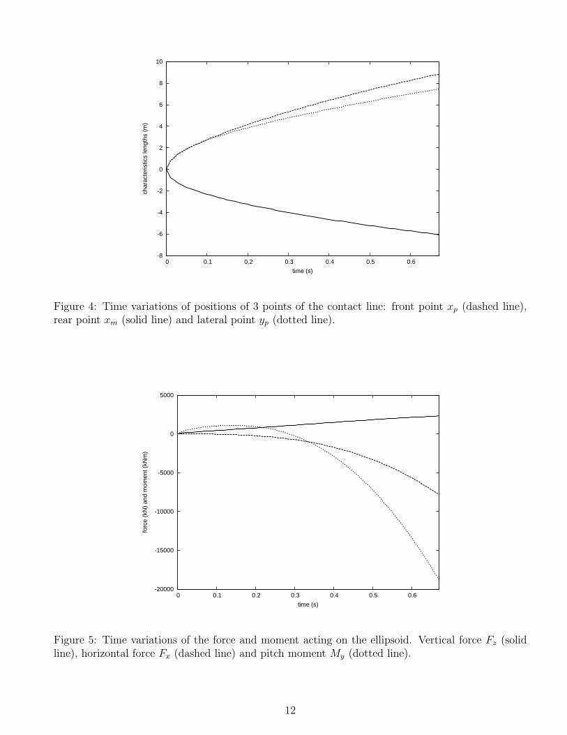
Calculations are performed for the ellipsoid with semi-axis a = 10m, b = 10m and c = 3m, whichis initially inclined at angle α0 = −6o. The ellipsoid moves with the horizontal speed 5m/s andpenetrates water at speed 1 m/s. The ellipsoid rotates with a constant angular velocity α(t) =α0 + αvt/T , where αv = 60 and T is chosen as 1s. These kinematics are arbitrary but satisfy thebasic assumptions of the model.

The positions of three points of the contact line, xm(t), xp(t) and yp(t), in the global coordinatesare shown in Figure (4). Here xm(t) and xp(t) are the maximum and minimum x− coordinates of

11

-8

-6

-4

-2

0

2

4

6

8

10

0 0.1 0.2 0.3 0.4 0.5 0.6

char

acte

ristic

s le

ngth

s (m

)

time (s)

Figure 4: Time variations of positions of 3 points of the contact line: front point xp (dashed line),rear point xm (solid line) and lateral point yp (dotted line).

-20000

-15000

-10000

-5000

0

5000

0 0.1 0.2 0.3 0.4 0.5 0.6

forc

e (k

N)

and

mom

ent (

kNm

)

time (s)

Figure 5: Time variations of the force and moment acting on the ellipsoid. Vertical force Fz (solidline), horizontal force Fx (dashed line) and pitch moment My (dotted line).

12

the contact line, and yp(t) is the y− semi-axis of the contact line. It is observed that the speed of therear point of the contact line xm(t) is zero at t = 0.67s, which is the duration of the Wagner stage ofimpact in the case under consideration (see § 5).

Equations (19) - (21), (44) - (45) provide the forces Fx(t), Fz(t) and the moment Mc(t) =zcFx − xcFz − My(t) with respect to the centre of the ellipsoid (see Figure 5) during the Wagnerstage, 0 < t < 0.67s. The vertical force Fz(t) is always positive and almost linear. The horizontalforce Fx(t) is negative and much greater than the vertical force at the end of the Wagner stage.The moment Mc(t) is positive for 0 < t < 0.3s while trying to increase the angle of the ellipsoidinclination, and negative after t > 0.3s while trying to sink the ellipsoid. In these calculations themotions of the body are prescribed.

7 Conclusion

Three-dimensional problem of water impact by a smooth body has been studied. The body moves insix degrees of freedom and changes its shape over time. The liquid flow and the pressure distributioncaused by the impact were obtained within the Wagner theory of water impact. Hydrodynamic forcesand moments acting on the body were derived in analytical form.

It was shown that water entry of a three-dimensional body moving with six degrees of freedomis rather different from pure vertical entry of the same body. Horizontal displacements of the bodyand its angular motions may lead to appearance of low-pressure zones in the wetted part of the bodysurface. These zones may expand in time and approach the periphery of the wetted area, which leadsto separation of the liquid surface from the surface of the body at the end of the impact stage of theentry. The present Wagner model fails when cavitation effects appear and when a zone of negativepressure arrives at the contact line. The horizontal velocity of the body can be much higher than itsvertical velocity within the present analysis.

The ditching of an aircraft is a particular application of the present theoretical study. Theditching involves mainly the heave, surge and pitch motions of the aircraft. It was shown that theactual shape of the aircraft fuselage can be approximated by an elliptic paraboloid close to the initialcontact point and the corresponding shape is characterized by time varying radii of curvature. Ifthe latter are large enough compared to the penetration depth, the Wagner theory provides reliableresults in terms of the loads.

Comparisons with experimental results for an oblique entry of an elliptic paraboloid support thepresent theoretical results for moderate horizontal velocities. In particular it is confirmed that anelliptic paraboloid entering an initially flat free surface with both horizontal and vertical velocitieshas an expanding wetted surface which is elliptic as well.

Acknowledgements

The present study is part of the TULCS project which received funding from the EuropeanCommunity’s Seventh Framework Programme under grant agreement number FP7-234146. Theexperimental programme is partly founded by Conseil General du Var (France). AK acknowledgesalso the support from EC PF7 project Smart Aircraft in Emergency Situations under the grantagreement number FP7-266172. AK is also thankful to the support by the NICOP research grant“Fundamental Analysis of the Water Exit Problem” N62909-13-1-N274, through Dr. Woei-Min Lin.Any opinions, findings, and conclusions or recommendations expressed in this material are those ofthe authors and do not necessarily reflect the views of the Office of Naval Research.

13

References

[Gradshteyn & Ryzhik (1994)] Gradshteyn, I.S. & Ryzhik, I.M. 1994 Tables of integrals 5th

edition, Academic Press, 1204pp.

[Howison et al.(1991)] Howison, S. D., Ockendon, J. R. & Wilson, S. K. 1991 Incompressiblewater-entry problems at small deadrise angles. J. Fluid Mech. , 222, 215-230.

[von Karman(1929)] von Karman, T. 1929 The impact of seaplane floats during landing. Technical

Notes NASA, 321.

[Kleefsman et al.(2005)] Kleefsman, K. M. T., Fekken, G., Veldman, A. E. P., Iwanowski,

B., & Buchner, B. 2005 A volume-of-fluid based simulation method for wave impact problems.Journal of Computational Physics , 206(1), 363-393.

[Kochin et al.(1964)] Kochin, N.E., Kibel, I.A., & Roze, N.V., 1964 Theoretical Hydrome-chanics. Intersciences Publishers.

[Korobkin(1985)] Korobkin, A.A. 1985 Initial asymptotics in the problem of blunt body entranceinto liquid. Ph.D thesis, Lavrentyev Institute of Hydrodynamics.

[Korobkin(2002)] Korobkin, A. A. 2002 The entry of an elliptical paraboloid into a liquid atvariable velocity. Journal of applied mathematics and mechanics , 66(1), 39-48.

[Korobkin(2005)] Korobkin, A. A. 2005 Three-dimensional nonlinear theory of water impact. In

18th International Congress of Mechanical Engineering, Ouro Preto, MG.

[Korobkin(2007)] Korobkin, A. A., 2007, Second-order Wagner theory of wave impact. J. Engng.

Math.,, 58(1-4), 121-139.

[Korobkin & Pukhnachov(1988)] Korobkin, A. A. & Pukhnachov V. V. 1988 Initial stage ofwater impact. Ann. Rev. Fluid Mech., 20, 159–185.

[Korobkin & Scolan(2006)] Korobkin, A. A., & Scolan, Y. M. 2006 Three-dimensional theoryof water impact. Part 2. Linearized Wagner problem. J. Fluid Mech., 549, 343-374.

[Korobkin(2013)] Korobkin, A. A. 2013 A linearized model of water exit. J. Fluid Mech., 737,368-386.

[Maruzewski et al.(2010)] Maruzewski, P., Touze, D. L., Oger, G., & Avellan, F. 2010SPH high-performance computing simulations of rigid solids impacting the free-surface of water.Journal of Hydraulic Research, 48(S1), 126-134.

[Molin et al.(1996)] Molin, B., Cointe, R. & Fontaine, E. 1996 On energy arguments appliedto the slamming force. Proc. 11th IWWWFB, Hamburg, Germany, 162-165.

[Moore et al.(2012)] Moore, M. R., Howison, S. D., Ockendon, J. R. & Oliver, J. M. 2012Three-dimensional oblique water-entry problems at small deadrise angles. J. Fluid Mech. , 711 ,259-280.

[Moore et al.(2013)] Moore, M. R., Howison, S. D., Ockendon, J. R. & Oliver, J. M. 2013A note on oblique water-entry. J. Engng. Math.,, 81(1), 67-74.

[Oliver(2007)] Oliver, J. M., 2007, Second-order Wagner theory for two-dimensional water-entryproblems at small deadrise angles. J. Fluid Mech., 572, 59-85.

14

[Scolan & Korobkin(2001)] Scolan, Y. M., & Korobkin, A. A. 2001 Three-dimensional theoryof water impact. Part 1. Inverse Wagner problem. J. Fluid Mech., 440(1), 293-326.

[Scolan & Korobkin(2003)] Scolan, Y. M., & Korobkin, A. A. 2003 Energy distribution fromvertical impact of a three-dimensional solid body onto the flat free surface of an ideal fluid. J.

Fluids and Structures, 17(2), 275-286.

[Scolan & Korobkin(2012)] Scolan, Y.-M. & Korobkin, A. A. 2012 Hydrodynamic impact(Wagner) problem and Galin’s theorem. In Proc. 27th IWWWFB, Copenhagen, Denmark, 165-168.

[Scolan & Korobkin(2012)] Scolan, Y.-M. & Korobkin, A. A. 2012 Low pressure occurrenceduring hydrodynamic impact of an elliptic paraboloid entering with arbitrary kinematics. InProc. 2nd Int. Conf. on Violent Flows, 1-8.

[Scolan(2012)] Scolan, Y.-M. 2012 Hydrodynamic loads during impact of a three dimensionalbody with an arbitrary kinematics (in french). Proc. 13th Journees de l’Hydrodynamique, Chatou,

France..

[Tassin et al.(2013)] Tassin, A., Piro, D. J., Korobkin, A. A., Maki, K. J., & Cooker, M.

J. 2013 Two-dimensional water entry and exit of a body whose shape varies in time. Journal of

Fluids and Structures, 40, 317-336.

[ Yang & Qiu(2012)] Yang, Q., & Qiu, W. 2012 Numerical simulation of water impact for 2D and3D bodies. Ocean Engineering , 43, 82-89.

[Wagner(1932)] Wagner, H. 1932 Uber Stoss- und Gleitvergange an der Oberflache von Flussig-keiten. ZAMM, 12 (4), 193-215.

15

8 Supplementary material: application of the model

That supplementary material contains an application of the model presented in the main body ofthe paper.

The 7 variables (h, Rx, Ry, αx, αy, xb, yb) completely define the state of the dynamical system.We consider the impact problem for a three-dimensional body, the radii of curvature of which aregiven functions of time Rx(t) = Rx(0) + Rx(0)t, Ry(t) = Ry(0) + Ry(0)t, where Rx(0) = 0.75m,Rx(0) = −4m/s, Ry(0) = 2m and Ry(0) = 30m/s. The body moves at speeds xb(t) = 7m/s,yb(t) = 2m/s, h(t) = 1m/s in the x−, y− and z−directions respectively. The angular velocitiesof the body are αx(t) = 1rd/s, αy(t) = 2rd/s. The aspect ratio kγ(t) =

√

Rx(t)/Ry(t) of the

horizontal sections of the body and the aspect ratio k(t) = a(t)/b(t) =√

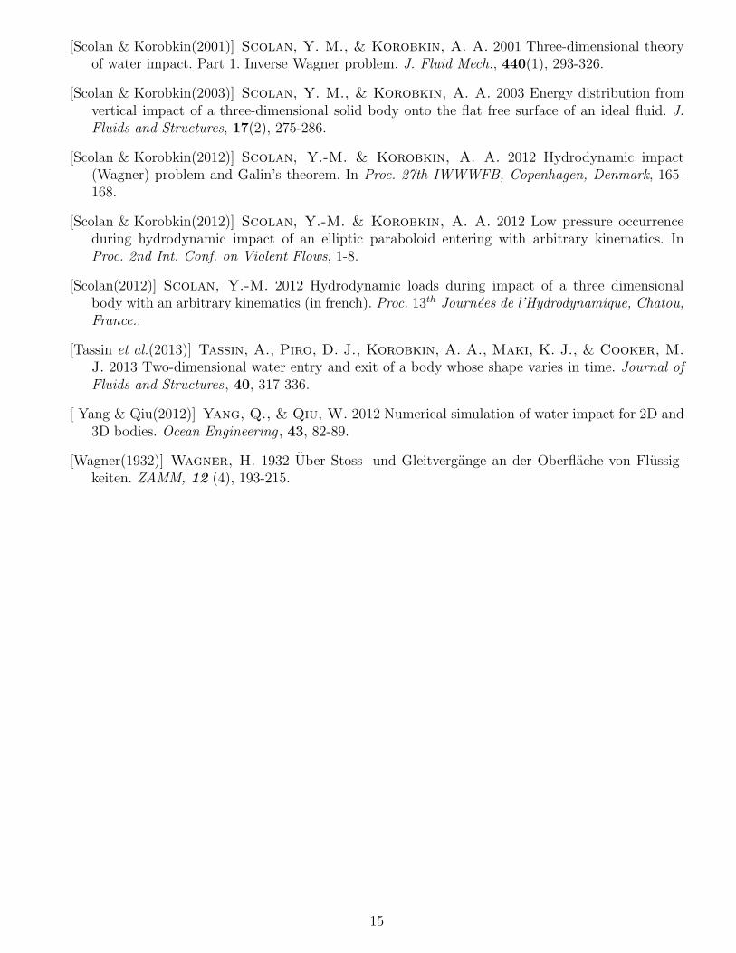
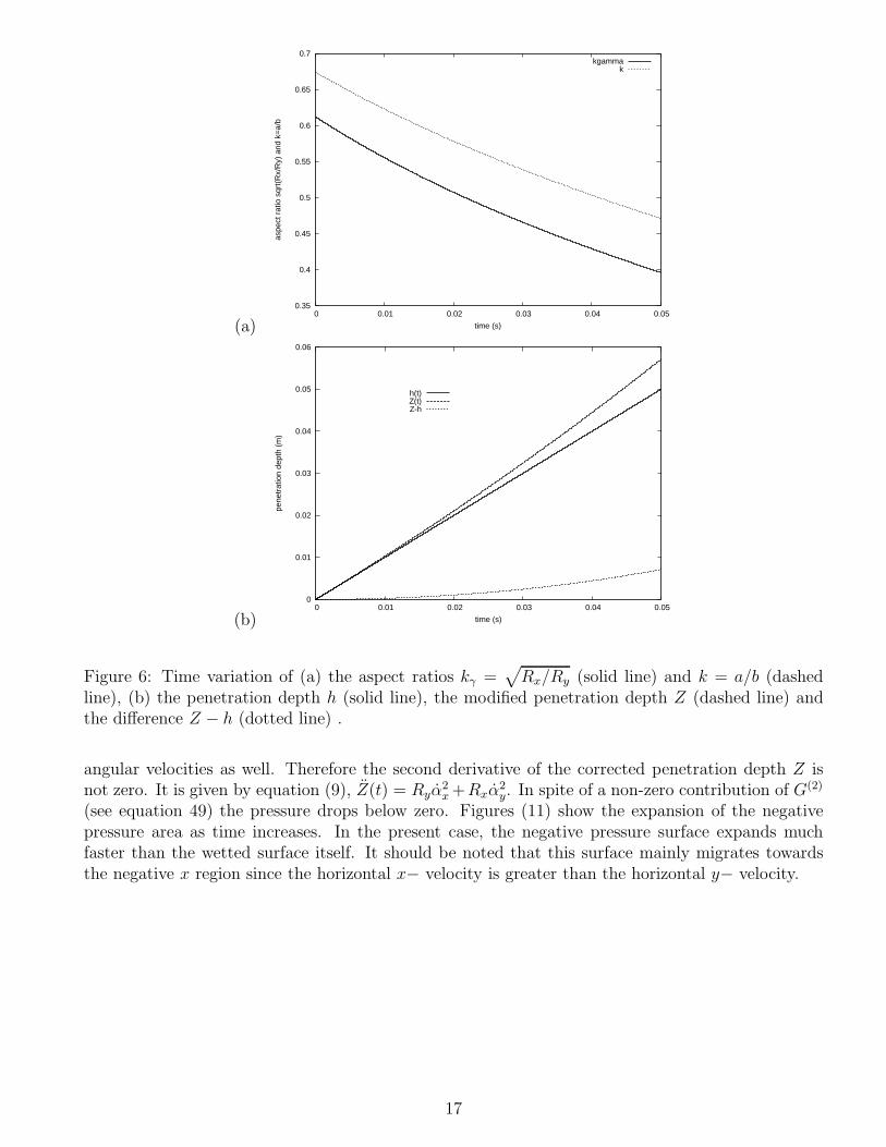
1 − e2(t) of the wettedsurface are shown in Figure (6a) as functions of time. The time simulation runs up to t = 0.05s. Themodified vertical displacement Z(t) of the body is given by equation (9) and shown in Figure (6b).It is observed that the modified penetration depth Z(t) is greater than the vertical displacement ofthe body h(t) = h(0)t. The Wagner line (periphery of the wetted surface) and the Karman line(intersection of the body with the undisturbed free surface) are computed and plotted in the globalcoordinate system in Figure (7a) for 0 < t < 0.05s. These lines for the vertical entry of the rigidbody (1 DoF) are shown in Figure (7b).

As expected, Figures (7) show that the surface made of all the Wagner lines overlaps the surfacemade of all the Karman lines. The effect of translational motion along the x and y axes, and thevariations of the curvature radii are noticeable. The configurations of the submerged body and therelated free surface deformation are shown in Figure (8). The free surface elevation in Figure (8) isgiven by [Korobkin & Scolan(2006)]

η(x, y, t) = − 1

2π

∫ ∫

D(t)

∆2φ(x0, y0, t)dx0dy0√

(x − x0)2 + (y − y0)2, ((x, y) ∈ FS(t)) , (48)

where ∆2φ is the planar Laplacian of the displacement potential in the wetted area. The integrationin (48) is performed numerically over the elliptic wetted surface D(t). It should be noted that wecannot expect any asymmetries of the free surface elevation around the body from the equation (48).The free surface pattern is only affected by the body rotations through the modified penetrationdepth Z(t), which is always greater than h(t) (see equation 9). However, it is not affected by thehorizontal motions of the body in the Wagner model.

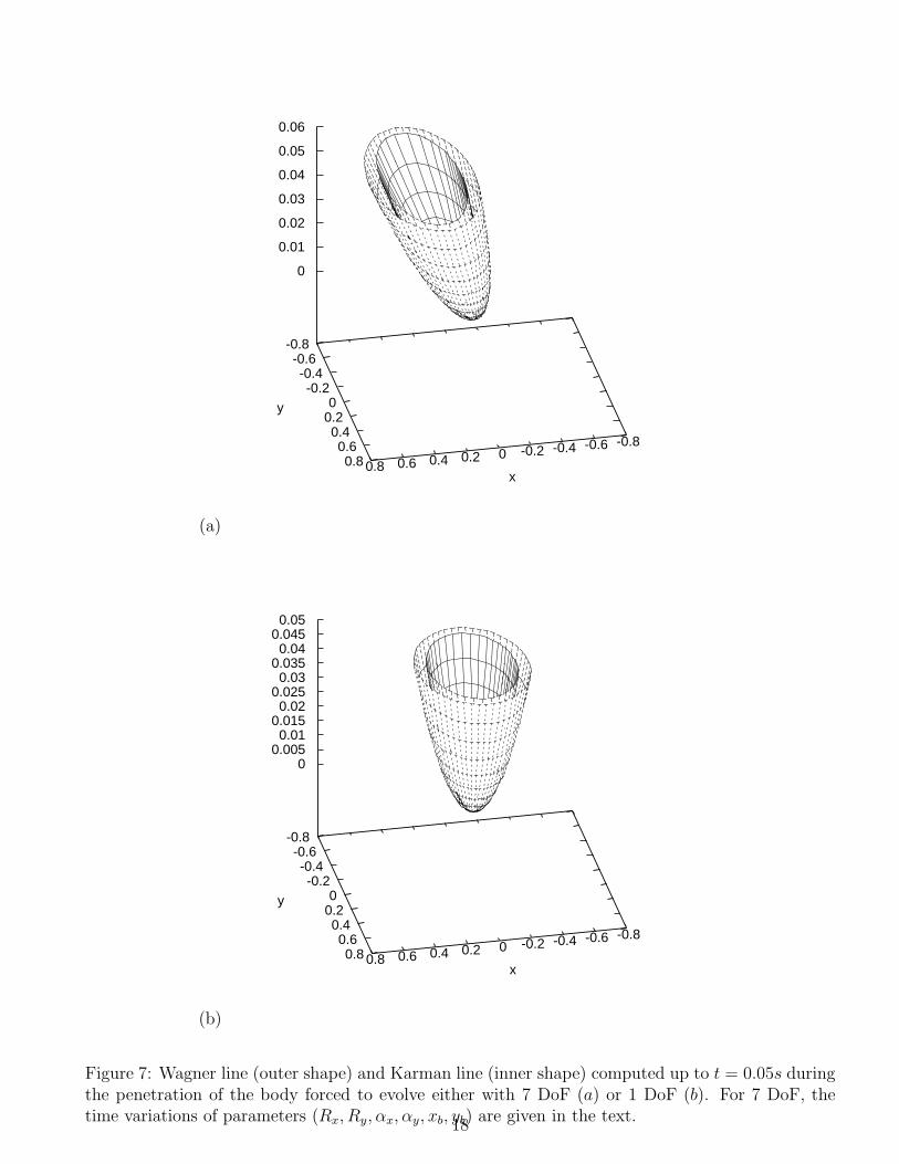
The force and moment components are computed by equations (19) and (20). The time variationsof (Fx, Fy, Fz, Mx, My) are plotted in Figure (9) for the simple vertical motion (1 DoF) and forthe complex kinematics (7 DoF). A parametric study of the influence of each degree of freedom(independently of the others) is performed. That study is not detailed here for sake of brevity. Itis remarkable that the vertical force is substantially increased compared to the 1 DoF case, mainlydue to the increasing curvature radii along the y direction. On the other hand the horizontal forceis comparable to the vertical force even though it increases more slowly with time.

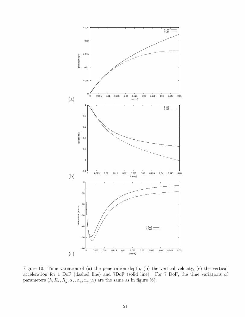
Free-drop penetration is considered next. Only the vertical motion is free while the horizontalmotions (xb, yb) are forced. The time variations of the parameters (Rx, Ry, αx, αy, xb, yb) are the sameas in Figure (6). The vertical kinematics are computed for the pure vertical motion (1 DoF) andfor the complex kinematics (7 DoF). The mass of the body is m = 10kg and its initial velocity ish(0) = 1m/s. Figures (10) show the time variations of the penetration depth, the velocity and theacceleration. The modification of the shape due to the change of the curvature radii is found to bethe main reason for the difference in kinematics.

The evolution of the negative pressure zone is illustrated in Figure (11) for a more general case.The body motions and deformation are governed by the same time variations as for Figure (6). Thevelocities in x, y and z directions are constant, and the body has angular motions with constant

16

(a)

0.35

0.4

0.45

0.5

0.55

0.6

0.65

0.7

0 0.01 0.02 0.03 0.04 0.05

aspe

ct r

atio

sqr

t(R

x/R

y) a

nd k

=a/

b

time (s)

kgammak

(b)

0

0.01

0.02

0.03

0.04

0.05

0.06

0 0.01 0.02 0.03 0.04 0.05

pene

trat

ion

dept

h (m

)

time (s)

h(t)Z(t)Z-h

Figure 6: Time variation of (a) the aspect ratios kγ =√

Rx/Ry (solid line) and k = a/b (dashedline), (b) the penetration depth h (solid line), the modified penetration depth Z (dashed line) andthe difference Z − h (dotted line) .

angular velocities as well. Therefore the second derivative of the corrected penetration depth Z isnot zero. It is given by equation (9), Z(t) = Ryα

2x +Rxα

2y. In spite of a non-zero contribution of G(2)

(see equation 49) the pressure drops below zero. Figures (11) show the expansion of the negativepressure area as time increases. In the present case, the negative pressure surface expands muchfaster than the wetted surface itself. It should be noted that this surface mainly migrates towardsthe negative x region since the horizontal x− velocity is greater than the horizontal y− velocity.

17

(a)

-0.8-0.6-0.4-0.2 0 0.2 0.4 0.6 0.8x

-0.8-0.6-0.4-0.2

0 0.2 0.4 0.6 0.8

y

0

0.01

0.02

0.03

0.04

0.05

0.06

(b)

-0.8-0.6-0.4-0.2 0 0.2 0.4 0.6 0.8x

-0.8-0.6-0.4-0.2

0 0.2 0.4 0.6 0.8

y

0 0.005 0.01

0.015 0.02

0.025 0.03

0.035 0.04

0.045 0.05

Figure 7: Wagner line (outer shape) and Karman line (inner shape) computed up to t = 0.05s duringthe penetration of the body forced to evolve either with 7 DoF (a) or 1 DoF (b). For 7 DoF, thetime variations of parameters (Rx, Ry, αx, αy, xb, yb) are given in the text.

18

(a)

-1.5 -1 -0.5 0 0.5 1 1.5x -1.5 -1 -0.5 0 0.5 1 1.5y

0

0.02

0.04

0.06

0.08

0.1

(b)

-1.5 -1 -0.5 0 0.5 1 1.5x -1.5 -1 -0.5 0 0.5 1 1.5y

0

0.02

0.04

0.06

0.08

0.1

Figure 8: Position of the body and corresponding free surface deformation for 7 DoF (a) and 1 DoF(b) at time t = 0.05s. For 7 DoF, the time variations of parameters (Rx, Ry, αx, αy, xb, yb) are givenin the text.

19

(a)

-3000

-2000

-1000

0

1000

2000

3000

4000

5000

6000

7000

0 0.01 0.02 0.03 0.04 0.05

forc

e (N

)

time (s)

Fx(t)Fy(t)Fz(t)

Fz(t) (1DoF)

(b)

-2500

-2000

-1500

-1000

-500

0

0 0.01 0.02 0.03 0.04 0.05

mom

ent (

Nm

)

time (s)

Mx(t)My(t)

Figure 9: Time variation of (a) horizontal and vertical forces for 7 DoF and 1 DoF, (b) moment aroundthe two horizontal axes. For 7 DoF, the time variations of parameters (h, Rx, Ry, αx, αy, xb, yb) arethe same as in figure (6).

20

(a)

0

0.005

0.01

0.015

0.02

0.025

0 0.005 0.01 0.015 0.02 0.025 0.03 0.035 0.04 0.045 0.05

pene

trat

ion

(m)

time (s)

1 DoF7 DoF

(b)

-0.2

0

0.2

0.4

0.6

0.8

1

0 0.005 0.01 0.015 0.02 0.025 0.03 0.035 0.04 0.045 0.05

velo

city

(m

/s)

time (s)

1 DoF7 DoF

(c)

-60

-50

-40

-30

-20

-10

0

0 0.005 0.01 0.015 0.02 0.025 0.03 0.035 0.04 0.045 0.05

acce

lera

tion

(m/s

**2)

time (s)

1 DoF7 DoF

Figure 10: Time variation of (a) the penetration depth, (b) the vertical velocity, (c) the verticalacceleration for 1 DoF (dashed line) and 7DoF (solid line). For 7 DoF, the time variations ofparameters (h, Rx, Ry, αx, αy, xb, yb) are the same as in figure (6).

21

-0.4

-0.2

0

0.2

0.4

-0.4 -0.2 0 0.2 0.4

y (m

)

x (m)

-0.4

-0.2

0

0.2

0.4

-0.4 -0.2 0 0.2 0.4

y (m

)x (m)

-0.4

-0.2

0

0.2

0.4

-0.4 -0.2 0 0.2 0.4

y (m

)

x (m)

-0.4

-0.2

0

0.2

0.4

-0.4 -0.2 0 0.2 0.4

y (m

)

x (m)

Figure 11: Successive plots of the contact line at time t = 0.010s, t = 0.011s, t = 0.012s andt = 0.013s. The surface of negative pressure is dark and the bigger ellipse gives the finite limit of theelliptic paraboloid. The curves are plotted in the coordinate system centered at (X, Y ). The timevariations of 7 parameters (Rx, Ry, αx, αy, h, xb, yb) are the same as for figure (6).

22