water contamination in the area of a landfill coal ash
TRANSCRIPT
WATER CONTAMINATION IN THE AREA OF A LANDFILL COAL ASH
Jean Marie SINZINKAYO
Dissertation submitted in fulfilment of the requirements for the degree of
MASTER IN MINING AND GEO-ENVIRONMENTAL ENGINEERING
Supervisor: Prof. Maria Cristina da Costa Vila
Co-Supervisor: Prof. Renata Maria Gomes dos Santos
Director of Master’s Programme: Prof. José Manuel Soutelo Soeiro de Carvalho
Examiner: Prof. Antonio Manuel Antunes Fiuza
NOVEMBER 2017

MASTER IN MINING AND GEO-ENVIRONMENTAL ENGINEERING 2016/2017
DEPARTMENT OF MINING ENGINEERING
Tel. +351 22 0413163/220413164
Edited by:
FACULDADE DE ENGENHARIA DA UNIVERSIDADE DO PORTO
Rua Dr. Roberto Frias
4200-465 Porto
Portugal
Tel. +351 22 508 1400
Fax +351 22 508 1440
Email [email protected]
URL http://www.fe.up.pt
Partial reproduction of this work is allowed as long as the Author is mentioned together with
the Master in Mining and Geo-Environmental Engineering – 2016/2017, Department of
Mining and Geo-Environmental Engineering, University of Porto – Faculty of Engineering
(Faculdade de Engenharia da Universidade do Porto - FEUP), Portugal 2017.
The opinions and information included herein solely represent the views of the Author and
the University may not accept legal responsibility or otherwise in relation to errors or
omissions that may exist.
This document was produced from an electronic copy provided by the Author.

i
Water Contamination in the Area of a Landfill Coal Ash
In God I Trust.

ii
Water Contamination in the Area of a Landfill Coal Ash
ABSTRACT
Water contamination is a threat to our lives on massive scale because it affects the food
chain. With the need of socio-economic development, anthropogenic activities such as,
mining and industries are severely affecting the aquatic ecosystem. Former mining plants and
industries used to stockpile waste and tailings or ashes on land and discharged leachates or
regeants into surface water.
The present work is the part of a broader research project which intended to analyze the
potential pollution caused by a landfill of coal ashes originated by an ancient coal power
station in northern Portugal.
The run off waters collected from a drainage piping system around the side-hills of the
storage (“fibrocimento tube”) are contaminated with heavy metals and its pH is in the range
of 2.9-5.4 revealing acid mine drainage generation.
The pollution is analyzed by implementing a transport model with advection, dispersive-
diffusion and degradation considering a first-order kinetics. The implementation of the
transport and fate model was performed both with Microsoft Excel and Matlab. The
simulation allowed to estimate the final concentrations of the contaminant at the discharge
point into Douro river. Comparison between these concentrations and the threshold limits for
emission of wastewater reveals that only manganese exceeds the threshold limit. The
decrease of the concentrations of contaminants is due to natural attenuation by clays natural
minerals and sorption into organic matter of the soil in the area.
Keywords: Heavy metals, Pollution, Landfill coal ash, Transport model, Water quality,
threshold value.

iii
Water Contamination in the Area of a Landfill Coal Ash
Résumé
La contamination de l'eau est une menace à grande échelle pour notre vie car elle affecte la
chaîne alimentaire. Les annciennes industries minières utilisaientt le stockage à decouvert
sur terre des déchets et résidus et deversaient les lixiviats dans les eaux de surface.
Le présent travail fait partie d'un projet de recherche plus large qui vise à analyser l'évolution
de la pollution causée par le dépôt de cendres de charbon d'une ancienne centrale
thermoélectrique dans la région de Medas de la municipalité de Gondomar au Portugal.
L'eau provenant de ce dépôt de cendres de charbon (tuyau Fibrocimento) est polluée par des
métaux lourds et son pH dans la gamme de 2,9-5,4 révèle la génération d’un drainage minier
acide. Cette évolution de pollution est analysée par un modèle de transport de l’ eau sur terre
en développant la première loi de Fick et en considérant la dégradation de premier ordre de
ces métaux lourds. L’ application de ce modèle de transport aux logiciels excel et matlab
déduit à la concentration finale de chaque méteau lourd dans l'eau déversée dans le fleuve
Douro. La comparaison des ces valeurs de concentration des metaux lourds avec la valeur
limite maximale de l'émission de résidus dans l'eau révèle que seule la concentration du
manganese dépasse la valeur limite admise. Le declin des valeurs de concentration des autres
metaux lourds est dû au phenomène d’attenuation naturelle des mineraux argileux et des
composés organiques du sol dans ces milieux.
Mots-clés: Métaux lourds, Pollution, dépôt de Cendres de charbon , Modèle de
transport ,Qualité de l'eau, valeur seuil.

iv
Water Contamination in the Area of a Landfill Coal Ash
ACKNOWLEDGEMENTS
I would like to express my gratitude to my supervisors Prof. Maria Cristina da Costa Vila and
Prof. Renata Maria Gomes dos Santos for their useful comments, remarks and scientific
rigors they addressed to me during this master thesis work.
Furthermore, I would like to address my special thanks to Prof. José Manuel Soutelo Soeiro
de Carvalho, Director of the master degree program for his kind guidance and advice from
the beginning of the learning process at University of Porto. I’m grateful to Prof. Antonio
Manuel Antunes Fiuza who willingly shared his precious time and knowledge during my
postgraduate studies at University of Porto.
I’m also very grateful to Father Paul Zingg of Schoenstatt community of Geneva for helping
me and providing me with funding during these days.
A very special gratitude goes to all Erasmus-Mundus/Kite project coordinators from whom I
owed the scholarship which allowed me to come to University of Porto.
My deep thanks are addressed to my late father who has gone before harvesting the fruits of
his effort to send me to school. I also thank my lovely Mother, my brothers, sisters and
nephews for their long prayers.
I thank greatly my family, my wife Gloriose NSHIMIRIMANA and my lovely daughter
Laena SINZINKAYO for their patience during my absence.
Student life abroad is not easy but I am lucky to have met Abel Cunha Rodrigues and Jorge
Mayer families who supported me during my stay in Portugal, many thanks go to them.
To the community of the Faculty of Engineering of the University of Porto I address my great
thanks.

v
Water Contamination in the Area of a Landfill Coal Ash
Dedication
I dedicate my dissertation to my wife Gloriose NSHIMIRIMANA and my dauther Laena
SINZINKAYO.
I also dedicate my work to my parents, especially my Mom, my brothers NDUWAYO
Laurent, GATOTO Audace and my sisters NDUWIMANA Yolande, NDIKUMUREMYI
Judith and NDAYIKENGURUKIYE Godeliève, my uncles and nephews.
To my friends and all those who support education for all, I dedicate my dissertation.

vi
CONTENT
ABSTRACT ................................................................................................................................................ ii
ACKNOWLEDGEMENTS .......................................................................................................................... iv
Dedication ............................................................................................................................................... v
LIST OF FIGURES ..................................................................................................................................... ix
LIST OF TABLES ....................................................................................................................................... xi
ACCRONYMS ......................................................................................................................................... xii
Chapter 1. Introduction .......................................................................................................................... 1
1.1. General Introduction ........................................................................................................................ 1
1.2. Objective of the dissertation ........................................................................................................... 1
1.3. Dissertation structure ...................................................................................................................... 2
1.4. Water ............................................................................................................................................... 2
1.5. Water quality ................................................................................................................................... 3
1.5.1. Water quality threshold limit value .............................................................................................. 4
1.5.2. Portugal water quality threshold value ........................................................................................ 5
1.6. Contamination/pollution ................................................................................................................. 6
1.6. 1.Water pollution ............................................................................................................................. 7
1.6.2. Water pollution sources ................................................................................................................ 7
1.7. Heavy metals pollution .................................................................................................................... 8
1.7.1. Heavy metal definition .................................................................................................................. 9
1.7.2. Heavy metals toxicity properties .................................................................................................. 9
1.7. 3. Source of heavy metals pollution .............................................................................................. 16
1.7.4. Fate of heavy metals as pollution ............................................................................................... 16
1.7.4.1 Pollution of aquatic life ............................................................................................................. 17
1.7.4.2. Acid mine drainage pollution ................................................................................................... 18
1.7.4.2.1. Chemistry of Acid Mine drainage.......................................................................................... 18
1.7.4.2.2. Effects of Acid Mine Drainage on aquatic life ....................................................................... 19
1.7.5. Heavy metals transport in water ................................................................................................ 20
I.8.Case study ........................................................................................................................................ 21
I.8.1. Douro River .................................................................................................................................. 23

vii
Chapter 2. DISSERTATION METHODOLOGY .......................................................................................... 24
2.1. Transport model application from Fibrocimento tube to Douro river .......................................... 24
2.1.1. Advection/convective process .................................................................................................... 24
2.1.2. Dispersion process ...................................................................................................................... 24
2.1.3. One-dimensional model within surface water ........................................................................... 24
2.1.4. Solution of the one-dimensional model ..................................................................................... 26
2.1.5. Solution of the equation taking into account of degradation .................................................... 26
2.1.5.1. Kinetic constant study .............................................................................................................. 27
2.1.5.1.1.Adsorption kinetic constant determination .......................................................................... 28
2.1.5.1.2. Natural clays for heavy metals adsorption ........................................................................... 28
2.1.5.1.3.Chitosan as natural occurring for Aluminum adsorption ...................................................... 29
2.1.5.2. Estimating Diffusion Coefficients in Aqueous Systems ............................................................ 30
2.2.Transport model implementation .................................................................................................. 32
2.2.1.Microsoft excel implementation protocol ................................................................................... 32
2.2.2.Matlab implementation protocol ................................................................................................ 33
2.2.2.1. Transport model-Time variable implementation protocol ...................................................... 33
2.2.2. 2.Transport model-Distance variable implementation protocol ................................................ 34
2.3. Available data ................................................................................................................................. 34
2.3.1 Data from monitoring field .......................................................................................................... 34
2.3.2. Calculated and converted dimensions ........................................................................................ 36
Chapter 3. RESULT AND DISCUSSION .................................................................................................... 37
3.1. Data analysis .................................................................................................................................. 37
3.2. Results ............................................................................................................................................ 37
3.2.1. Results from Microsoft excel implementation ........................................................................... 38
3.2.1.1. Results from Microsoft excel for transport model-time evolution with degradation from the
source .................................................................................................................................................... 38
3.2.1.2.Results from Microsoft excel for transport model- distance evolution with degredation
fromthe source ..................................................................................................................................... 50
3.2.2. Results from matlab implementation ......................................................................................... 62
3.2.2.1. Matlab results for a transport model- time evolution with degradation from the source ..... 63
3.2.2.2 Matlab results for a transport model-distance evolution with degradation from the source . 67

viii
3.3.Microsoft-Excel and matlab cross validation .................................................................................. 71
3.4. Discussion ....................................................................................................................................... 72
3.4.1. Toxicity caused by the concentration of heavy metals in water ................................................ 72
3.4.2.Acidity of water caused by the AMD ........................................................................................... 73
3.4.3. Natural attenuation of heavy metals .......................................................................................... 74
3.4.4.Natural attenuation of AMD and pH buffering ............................................................................ 74
3.4.4. 1.Authigenic secondary minerals formation ............................................................................... 74
Chapter 4 : CONCLUSION AND RECOMMENDATIONS .......................................................................... 76
4.1. Conclusion ...................................................................................................................................... 76
4.2. Recommendations for future works .............................................................................................. 76

ix
LIST OF FIGURES Figure 1: Water distribution in the world ........................................................................................ 3
Figure 2: Acute (a) and chronic (b) poisoning effects of copper .................................................. 13
Figure 3:Comparison of the effects of zinc intoxication versus deficiency .................................. 15
Figure 4 : Source of heavy metals pollution ................................................................................. 16
Figure 5: Dead fish by AMD effect .............................................................................................. 20
Figure 6: Map of the study area .................................................................................................... 21
Figure 7: Aspect of water collection system on the study area ..................................................... 22
Figure 8: Tubular reactor .............................................................................................................. 25
Figure 9:Graphic of aluminum transport model- time evolution .................................................. 39
Figure 10:Graphic of the fifth curve of the aluminum transport model-time evolution ............... 40
Figure11: Graphic of copper transport model-time evolution ...................................................... 40
Figure12: Graphic of the fith curve of copper transport model-time evolution ............................ 41
Figure 13: Graphic of iron transport model-time evolution .......................................................... 42
Figure 14: Graphic of the fith curve of iron transport model-time evolution ............................... 43
Figure 15: Graphic of manganese transport model-time evolution ............................................... 43
Figure 16: Graphic of the fith curve of manganese transport model-time evolution .................... 44
Figure 17: Graphic of zinc transport model-time evolution .......................................................... 45
Figure 18: Graphic of the fith curve of zinc transport model-time evolution ............................... 46
Figure 19: Graphic of arsenic transport model-time evolution ..................................................... 46
Figure 20: Graphic of the fith curve of arsenic transport model-time evolution .......................... 47
Figure 21: Graphic of nickel transport model-time evolution....................................................... 48
Figure 22 : Graphic of the fith curve of nickel transport model-time evolution ........................... 49
Figure 23: Graphic of lead transport model-time evolution .......................................................... 49
Figure 24: Graphic of the fith curve of lead transport model-time evolution ............................... 50
Figure 25: Graphic of aluminum transport model-distance evolution .......................................... 51
Figure 26: Graphic of the sixth curve of aluminum transport model-distance evolution ............. 52
Figure 27: Graphic of copper transport model- distance evolution .............................................. 52
Figure 28: Graphic of the sixth curve of copper transport model-distance evolution ................... 53
Figure 29: Graphic of iron transport model-distance evolution .................................................... 54
Figure 30: Graphic of the sixth curve of iron transport model-distance evolution ....................... 55

x
Figure 31: Graphic of manganese transport model-distance evolution ......................................... 55
Figure 32: Graphic of the sixth curve of manganese transport model-distance evolution ............ 56
Figure 33: Graphic of zinc transport model-Distance evolution ................................................... 56
Figure 34: Graphic of the sixth curve of zinc transport model-distance evolution ....................... 57
Figure 35: Graphic of arsenic transport model-Distance evolution .............................................. 58
Figure 36: Graphic of the sixth curve of arsenic transport model-distance evolution .................. 59
Figure 37: Graphic of nickel transport model-distance evolution................................................. 59
Figure 38: Graphic of the sixth curve of nickel transport model-distance evolution .................... 60
Figure 39: Graphic of lead transport model-distance evolution .................................................... 60
Figure 40: Graphic of the sixth curve of lead transport model-Distance evolution ...................... 61
Figure 41: Aluminum transport model-time evolution graphic from matlab ................................ 63
Figure 42: Iron transport model-time evolution graphic from matlab .......................................... 63
Figure 43: Copper transport model-time evolution graphic from matlab ..................................... 64
Figure 44: Manganese transport model-time evolution graphic from matlab ............................... 64
Figure 45: Zinc transport model-time evolution graphic from matlab .......................................... 65
Figure 46: Arsenic transport model-time evolution graphic from matlab .................................... 65
Figure 47: Nickel transport model-time evolution graphic from matlab ...................................... 66
Figure 48: Lead transport model-time evolution graphic from matlab ......................................... 66
Figure 49: Aluminum transport model- distance evolution graphic from matlab ......................... 67
Figure 50: Copper transport model- distance evolution graphic from matlab .............................. 67
Figure 51: Iron transport model- distance evolution graphic from matlab ................................... 68
Figure 52: Manganese transport model- distance evolution graphic from matlab ........................ 68
Figure 53: Zinc transport model- distance evolution graphic from matlab ................................... 69
Figure 54: Arsenic transport model- distance evolution graphic from matlab.............................. 69
Figure 55: Nickel transport model- distance evolution graphic from matlab ............................... 70
Figure 56: Lead transport model- distance evolution graphic from matlab .................................. 70

xi
LIST OF TABLES Table 1: Limit values of emission of some chemicals in water 5
Table 2: First order kinetic constant of heavy metals/chemicals removal in water 30
Table 3 : Diffusivity coefficient estimation 31
Table 4: Concentration and pH of heavy metals and sulfide at Fibrocimento source, in Douro
surface water and at 2.5m deep in water. 35
Table 5: Characteristic of the tube 36
Table 6: Simulated residence time and predicted values of concentration from excel implementation
of each chemical getting into Douro river 62
Table 7: Simulated residence time and predicted values of concentration of heavy metals and other
chemicals discharged into Douro river from matlab implementation 71
Table 8: Excel and Matlab cross validation values 72
Table 9: Comparison of predicted values of concentration discharged into Douro river to the
threshold limit values 73

xii
ACCRONYMS
AMD: Acid Mine Drainage
UNEP: United Nation for Environment Protection
UNESCO: United Nations Educational, Scientific and Cultural Organization
WHO: World Health Organization
EPA: Environmental Protection Agency
ACGH: American Conference of Government Industrial Hygienists
EC: European Commission
DL: Diario da Republica
DNA: Deoxyribonucleic Acid
TDS: Total Dissolved Solids
ROS: Reactive Oxygen Species
MCV: Mean Corpuscular Volume
MCH: Mean Corpuscular Hemoglobin
MCHC: Mean Corpuscular Hemoglobin Control
VMA: Valeur minimum admise (in French language)
MAV: Minimum Admited Value (in English language)
TPP: Thermo-Electric Power Plant
MW: Megawatt
°C: Celsius Degree
N: North
W: West
Å: Angstrom
ARDS: Adult Respiratory Distress Syndrome
Eh: Redox potential
pH: Hydrogen Potential

1
Chapter 1. Introduction
1.1. General Introduction
With the need of socio-economic development all over the world, adverse effects of
anthropogenic activities on natural ecosystem are severely enormous. Anthropogenic
activities such as mining and industrial activities threaten the environment.
The main part of the natural ecosystem threatened by such activities are air, soil and water.
Water is the lifeblood of our planet. It is fundamental to the biochemistry of all living
organisms. The earth’s ecosystems are linked and maintained by water, and provide a
permanent habitat for many species, including some 8.500 species of fishes (Acreman, 2004).
It is important for human to have an ability to control and protect such systems.
In former mining plants, waste, residues or ashes were stockpiled on land and leachates or
reagents were discharged into natural water without taking into consideration their
environmental impacts.The stockpiled waste, residues or ash were percolated by rain water
and their leachate was directed into surface water.
Some researches and studies should be conducted in order to assess the risk of water
pollution.
1.2. Objective of the dissertation
The objective of this work is to analyse the evolution of pollution generated by a landfill coal
ash to Douro river.
Using a computational model with microsof-excel and matlab, this work emphasizes on the
following specific objectives:
To determine by plotting a transport model, the predicted concentration of heavy metals or
chemicals discharged into Douro river;
To compare the concentration of heavy metals or other chemicals in water discharged into
Douro river and the maximum admited value of emission of residues to water decreed by the
Government of Portugal; and hence make a conclusion on the potential pollution of Douro
river;
To determine the time at which heavy metals or chemicals start to dissolve, at a certain pick
of maximal concentration;

2
To determine the simulated residence time of each heavy metals or chemicals during the
pathway from Fibrocimento to Douro river.
To estimate other parameters influencing the transport model such as kinetic and diffusivity
constants.
1.3. Dissertation structure
This dissertation is organized in four chapters, references and annex.
The chapter 1 consists of the introduction which relates the objective of this work and
provides definitions of some related concepts;
The chapter 2 describes the methodology used in analysing the evolution of pollution of the
land fill coal ash to Douro River;
The chapter 3 deals with results and discussion;
The chapter 4 presents conclusion of the dissertation and the recommendations for future
works;
The annex presents tables of the results from calculations.
1.4. Water
Of all the water on Earth, only 3% is present as freshwater in lakes, rivers , groundwater
(figure 1) and reservoirs systems where it is most easily accessible for use (Krantzberg et al.,
2010).
Water covers about 70% of Earth’s surface, makes up about 70% of our mass body, and is
essential for life (Shakhashiri, 2011).
Water is part of the physiological process of nutrition and waste removal from cell of all
living organisms. It is one of the controlling factors for biodiversity and the distribution of
Earth’s varied ecosystems, communities of animals, plants, bacteria and their interrelated
physical and chemical environments (Vandas et al., 2002).
Water on Earth’s surface, surface water, exists as streams, rivers, lakes and wetlands, as well
as bays and oceans. Surface water also includes the solid forms of water, snow and ice. Water
below the surface of the Earth primarily is groundwater, but it also includes soil water (Alley
et al., 1998).

3
Aquatic systems, such as wetlands, streams, rivers and lakes are especially sensitive to
changes in water quality and quantity. These ecosystems receive sediments, nutrients, and
toxic substances that are produced or used within their watershed, the land area that drains
water to stream, river, lake or ocean. Thus, an aquatic ecosystem is indicative of the
conditions of the terrestrial habitat in its watershed (Vandas et al., 2002).
Figure 1: Water distribution in the world (Krantzberg et al., 2010)
1.5. Water quality
Water quality is defined as suitability of water to sustain various uses or processes. Any use
will have certain requirements for the physical, chemical or biological characteristics,
example, limits on the concentrations of toxic substances, restrictions on temperature and pH
ranges for water supporting invertebrate communities. Consequently, water quality can be
defined by a range of variables which limit its use (Bartra & Ballance, 1996).
Krantzberg et al., (2010) consider that water quality is commonly defined by its physical,
chemical, biological and aesthetical characteristics and reflects its composition as affected by
nature and human activities.
A healthy environment is thus one in which water quality supports a rich and varied
community of organisms and protects public health.
Many aspects of water quality are developed. Chapman, (1996) considers water quality
within the aquatic environment and generally defines aquatic environment as:

4
Set of concentrations, speciation, and physical partitions of inorganic or organic
substances.
Composition and state of aquatic biota in the water body.
Description of temporal and spatial variations due to internal and external factors to
water body.
Water quality can hence be defined considering the environmental area because physical,
chemical and biological properties vary in space and time due to natural and anthropogenic
activities.
With the aim of protection of public health, UNEP, UNESCO, WHO, EPA, environmental
experts, government authorities and other organisms over the world created a lot of strategies
to combat water quality deterioration. Some are adopted as water quality guidelines, water
quality objectives, water quality criteria and water quality standards.
Water quality criteria and water quality standards are related and serve as a baseline for
establishing water quality objectives in enforceable environmental control laws or
regulations, while water quality objectives are defined as numerical and narrative statements
established to support and protect water uses (Helmer & Hespanhol, 1997).
Water quality criteria are synonyms to water quality guidelines and define technically-
derived numerical measures of concentrations or descriptive statements to protect aquatic
ecosystems and human water uses. They are hence derived from a range of physico-chemical,
biological and habitat indicators based on best-available science.
All those strategies are hence base line of water quality guidelines and those numerical values
are defined as quantitative measures that protect the environment. Those values are known as
threshold values. A definition of threshold value is given below.
1.5.1. Water quality threshold limit value
Threshold limit value started in 1942 when an American Conference of Government
Industrial Hygienists (ACGIH) committee was created to compile a listing of state
government exposure limits to various chemicals. The committee published then its first
annual list of recommended “Maximum allowable concentration” for 144 substances ; thus ,
the primary source for the term “Threshold limit value” (Ziemen & Castleman, 1989).
Several definitions have been developed after. Based on an ecological point of view,
threshold is the point at which there is an abrupt change in an ecosystem quality, property or

5
phenomenon, where small changes in an environmental driver produce large responses in the
ecosystem (Groffman et al., 2006).
1.5.2. Portugal water quality threshold value
Based on the previous definitions of water quality, each country or organization adopts
directives to protect water against pollution and deterioration. An example is the Directive
2006/118/EC of European Union which stipulates: “Having regard to the need to achieve
consistent levels of protection for groundwater, quality standards and thresholds values
should be established, and methodologies based on a common approach developed, in order
to provide criteria for the assessment of the chemical status of groundwater bodies”
(Directive 2006/118/EC, 2006).
In Portugal, the first regulations in the XX th century related to water quality date from 1904.
At the moment the standards that regulate the quality of water are given in a Law (DL
306/2007) that was published in 2007 and transpose the European Directive. That law
replaces the standards established in 2001 (DL243/2001) that in turn, replaces the standards
established in 1998 (DL 236/98).
The limit value of emission of chemicals used in this work (table1) are found in (DL 236/98).
Table 1: Limit values of emission of some chemicals in water (DL 236/98, 1998).
Chemicals Limit value of
emission (mg/l)
Al 10
Fe 2.0
Mn 2.0
Ni 2.0
As 1.0
Pb 1.0
Cu 1.0
Zn 0.5
The ministry of Environment of Portugal approved also that the minimal limit value of pH of
residues allowed to be discharged into water is in the range of 5.0-9.0 (DL 236/98, 1998).

6
1.6. Contamination/pollution
Contamination and pollution have different meanings even though they have been used as
identical terms for a long time. Some environmental experts try to provide different
definitions but there is still confusion in using them. It is then necessary to make a distinction
between them. What is more important for both terms is that they are applicable to water
quality degradation.
Contamination is defined as an introduction into water of any substance in undesirable
concentration not normally present in water, e.g. microorganisms, chemicals, waste or
sewage, which renders the water unfit for its intended use, and pollution is an addition of
pollutant to water while pollutant is defined as substance which impairs the suitability of
water for a considered purpose (UNESCO, 1992 in Zaporozec, 2002).
Those definitions are similar and Zaporozec, (2002) continues in the same way by giving a
very short and strait definitions. He defines contaminant as a naturally-occurring or human-
produced substance that renders water unfits for a given use, and pollution is an addition of
pollutant to water which restrains its use.
Based on those definitions, Zaporozec, (2002) considers that those terms are similar and
based on degradation of water quality for a given use.
Other environmental experts consider futhermore the harmful effects to human health.
Contamination is simply the presence of a substance where it should not be or at
concentration above background. Pollution is contamination that results in or can result in
adverse biological effects to communities. All pollutants are contaminants, but not all
contaminants are pollutants (Chapman, 2007).
Chapman, (2007) points out that the task of differentiating pollution from contamination is
not easy as it can also not be done solely based on chemical analysis because such analyses
cannot provide information on bioavailability or on toxicity. Effects based measures such as
laboratory or field toxicity tests and measures of the status of resident, exposed communities
provide key information, but cannot be used independently to determine pollution status,

7
because measures cannot easily distinguish between adaptation to contamination (a genetic
process) and acclimation1. Contaminant effects may not be only direct but also indirect.
From Chapman, (2007) consideration, there is distinction between pollution and
contamination. But to make it, it is better to consider a large scale of affected communities
because there should occur adaptation.
Pollution is hence contamination at large and deep scale with biological effects on affected
communities. In this work, pollution is used as an environmental threat.
1.6. 1.Water pollution
Polluted water may have undesirable color, odor, taste, turbidity, organic matter contents,
harmful chemical contents, toxic and heavy metals, pesticides, oily matters, industrial waste
products, radioactivity, high Total Dissolved Solids (TDS), acids, alkalis, domestic sewage
content, virus, bacteria, protozoa, rotifers, worms, etc.
Polluted surface waters (rivers, lakes, and ponds), groundwater, and sea water are all harmful
for human, animals and aquatic life (Trivedi, 2003).
In aquatic systems, pollutants are classified in four categories (Rico et al., 1989):
1. Those reaching the environment in enormous quantities;
2. Those which are toxic to aquatic organisms;
3. Those which can be concentrated within organisms to the levels greater than in their
living medium and;
4. Those persistent for long period with a high biological half-life.
Among those four categories, heavy metals can be classified into more than one category.
1.6.2. Water pollution sources
All environmental experts point out that water pollutant sources are categorized as point and
non-point sources. But there is an ambiguity in making distinction between them. Chapman,
(1996) defines a non-point source as a diffuse sources. He argues that a diffuse source on a
1 According the environmental Engineering Dictionary, acclimation is the response by an animal that enable it
to tolerate a change in a single factor ( e.g. temperature) in its environment (Mehdi & Agency, 2008), it can also
be a tolerance or adaptation of species to toxic metal concentration (Muyssen & Janssen, 2001).

8
regional or even local scale may result from a large number of individual point sources, e.g.
an automobile exhausts. The important difference between a point and non-point source is
that a point source may be collected, treated or controlled. A diffuse source resulting from
many point sources may be controlled provided that all point sources can be identified. He
says that the major point sources of pollution to fresh water originate from the collection and
discharge of domestic waste water, industrial wastes or certain agricultural activities such as
animal husbandry, and most other agricultural activities, such as pesticide spraying or
fertilizer application are considered as diffuse sources.
In their distinction, Loague & Corwin, ( 2016) involve more deeply some other aspects. They
characterize a point source as i) easier to control, ii) more readily identifiable and measurable
and iii) generally more toxic. They define a non-point source of pollution as the consequence
of agricultural activities (e.g. irrigation and drainage, application of pesticides and fertilizers,
run off and erosion); urban and industrial run off, erosion associated with construction,
mining and forest harvesting activities, lawns, roadways, and golf courses, road salt run off,
atmospheric deposition, livestock waste, and hydrologic modification (e.g. dams, diversions,
channelization, over pumping of ground water and siltation). They also consider that a point
source includes hazardous spills, underground storage tanks, storage piles of chemicals,
mine-waste ponds, deep-well waste disposal, industrial or municipal waste outfalls, run off,
and leachate from municipal and hazardous waste dumpsites and septic tanks. They
characterize a non-point source as i) difficult or impossible to trace ii) enter the environment
over an extensive area and sporadic timeframe; iii) are related (at least in part) to certain
uncontrollable meteorological events and existing geographic/geomorphologic conditions, iv)
have the potential for maintaining a relatively long active presence on the global ecosystem,
and v) may result in long-term, chronic (and endocrine) effects on human health and soil-
aquatic degradation.
From the previous definitions, it is possible to deduce that point and non-point source can
both be more toxic but the main difference between them is that a non-point source is diffuse
and a point source is non-diffuse.
1.7. Heavy metals pollution
Some heavy metals have bio-importance as trace elements (Duruibe et al., 2007), but at a
certain concentration level, the bio-toxic effects of many of them are harmful to aquatic live
and human health.

9
It is then necessary to know the properties of those natural and anthropogenic occurring and
understand their related impact on environment.
1.7.1. Heavy metal definition
Heavy metals refer to any metallic element that has a relatively high density. Heavy metal is
a general collective term, which applies to the group of metals and metalloids with a density
greater than 4g/cm3 or five times or more greater than the density of water (Dipak, 2017).
Heavy metals include lead (Pb), cadmium (Cd), zinc (Zn), mercury (Hg), arsenic (As), silver
(Ag), chromium (Cr), copper (Cu), iron (Fe), and the platinum group elements. Heavy metals
are toxic even at low concentration. They occur as natural constituents of the earth crust, and
are persistent environmental pollutant since they cannot be degraded or destroyed. To a small
extent, they enter the body system through food, air, and water, and bio-accumulate over a
period of time (Duruibe et al.,2007).
1.7.2. Heavy metals toxicity properties
Heavy metals are significant environmental pollutants and their toxicity is a problem of
increasing significance for ecological, evolutionary, nutritional and environmental reasons.
Heavy metals toxicity can lower energy levels and damage the function of the brain, lungs,
kidney, liver, blood composition and other important organs. Long-term exposure can lead to
gradually progressing physical, muscular, and neurological degenerative process that initiate
diseases such as multiple sclerosis, Parkinson’s disease, Alzheimer’s disease and muscular
dystrophy. Repeated long-term exposure of some heavy metals may even cause cancer
(Jaishankar, Tseten, Anbalagan, Mathew, & Beeregowda, 2014).
Symptoms that arise as a result of metal poisoning include intellectual disability in children,
dementia in adults, central nervous system disorders, insomnia, emotional instability,
depression and vision disturbances (Jan et al., 2015).
The following properties are related to heavy metals which are the main pollutants on which
this work emphasizes.
Arsenic(As)
Arsenic is one of the most important heavy metals causing disquiet from both ecological and
individual health standpoints. It is prominently toxic and carcinogenic, and extensively
available in the form of oxides, sulfides or as a salt of iron, sodium, calcium, copper, etc.

10
Arsenic is the twentieth most abundant element on earth and its inorganic forms such as
arsenate and arsenite compounds are lethal to the environment and human life. Deliberate
consumption of arsenic in case of suicidal attempts or accidental consumption by the children
may also result in cases of acute poisoning (Jaishankar et al., 2014).
Most common arsenic compounds occur in three oxidation states: trivalent arsenite,
pentavalent arsenate and elemental arsenic. Arsenite is ten times more toxic than arsenate,
and elemental arsenic is nontoxic. Arsenic also exists in three chemical forms: organic,
inorganic and arsine gas. Organic arsenic is having little acute toxicity whereas inorganic
arsenic and arsine gas are toxic (Ibrahim et al., 2006).
Arsenic is a protoplasmic poison since it affects primarily the sulfhydryl group of cells
causing malfunctioning of cell respiration, cell enzymes and mitosis (Saha et al., 1999).
The inhalation and ingestion of arsenic cause acute effects as mucosal damage, hypovolemic
shock, fever, sloughing, gastro-intestinal pain and anorexia. The chronic effects of arsenic are
weakness, hepatomegaly, melanosis, peripheral neuropathy, peripheral vascular disease,
carcinogenicity, liver, skin and lung cancer. As a health effects, arsenic causes gastro
intestinal damage, severe vomiting and death (Jan et al., 2015).
Low levels exposure to arsenic can cause nausea and vomiting, decreased production of red
and white blood cells, abnormal heart rhythm, damage to blood vessels, and a sensation of
“pins and needles in hands and feet”. Ingestion of very high levels can possibly result in
death. Long term low level exposure can cause darkening of the skin and the appearance of
small “corns” or “ warts” on the palms, soles and torso (Wendy & Sabine, 2009).
Lead(Pb)
Lead has no known beneficial effects in human body. Lead is a highly toxic metal whose
widespread use has caused extensive environmental contamination and health problems in
many parts of the world. Lead is a bright silvery metal, slightly bluish in a dry atmosphere. It
begins to tarnish on contact with air, by forming a complex mixture of compounds,
depending on the given conditions. Lead is an extremely toxic heavy metal that disturbs
various plants, physiological processes and unlike other metals, such as zinc, copper and
manganese, it does not play any biological functions. A plant with high lead concentration
speeds up the production of reactive oxygen species (ROS), causing lipid membrane damage
that ultimately leads to damage of chlorophyll and photosynthetic process and suppresses the
overall growth of the plant (Hou et al., 2013).

11
Lead enters in the human body by inhalation and ingestion. Lead has the acute effects of
nausea, vomiting, thirst, diarrhea, constipation, abdominal pain, hemoglobinuria, oliguria
leading to hypovolemic shock. The chronic effects of lead are colic, palsy and
encephalopathy. Its health effects are anemia, hypertension, kidney damage, disruption of
nervous systems, brain damage and intellectual disorders (Jan et al., 2015).
For pregnant women, exposure to high level of lead my cause miscarriage, and for men it
causes damage of organs responsible for sperm production and finally causes infertility
(Wendy & Sabine, 2009).
Aluminum(Al)
Investigations on environmental toxicity revealed that aluminum may present a major treat to
humans, animals and plants in causing many diseases. Many factors, including pH of water
and organic matter content, greatly influence the toxicity of aluminum.With decreasing pH,
its toxicity increases. Aluminum in high concentrations is very toxic for aquatic animals,
especially for gill breathing organisms such as fish, causing osmoregulatory failure by
destroying the plasma and hemolymph ions. The activity of gill enzyme, essential for the
uptake of ions, is inhibited by monomeric form of aluminum in fish. Living organisms in
water, such as seaweeds and grawfish, are also affected by its toxicity (Jaishankar et al.,
2014).
The aluminum toxicity in human body is related to renal osteodystrophy and dialysis
encephalopathy (King et al., 1981).
Iron(Fe)
Iron is an essential nutrient for most living organisms because it is a component or cofactor of
many critical proteins and enzymes. Iron toxicity is related to the generation of free radicals.
Both normal and pathogic cellular processes produce superoxide (O2-) and hydrogen peroxide
(H2O2) byproducts, whereas enzymes such as super oxide dismutase, glutathione peroxidase,
and catalase normally metabolize and neutralize these free radicals.One of the effects of (O2-)
is the release of stored iron from ferritin. The free iron reacts with (O2- ) and (H2O2) to
produce other more reactive and toxic-free radicals such as hydroxyl radical.The hydroxyl
radical can depolymerize polysaccharides, cause DNA strand breaks, inactive enzymes, and
irritate lipid peroxidation which amplify damaging cellular and subcellular membranes. If the
damage is not repaired, it can lead to cell death (Jeffrey, 2000).

12
The abundance of species such as periphyton, benthic invertebrates and fish diversity are
greatly affected by the direct and indirect effects of iron contamination. The iron precipitate
causes considerable damage by means of clogging action and hinder the respiration of fishes.
(Jaishankar et al., 2014).
Copper (Cu)
Even copper is an essential trace metal and micronutrient for cellular metabolism on living
organisms in account of being a key constituent of metabolic enzymes (Badiye et al., 2013), it
can however be extremely toxic to human body and cause acute and chronic poisoning
(figure 2 a and b respectively).
It is also toxic to intracellular mechanisms in aquatic animals at high concentrations when it
exceeds the threshold level. Fish can accumulate copper via diet or ambient exposure. Even at
low environmental concentrations, copper shows distinct affinity to accumulate in fish liver.
The typical patho-anatomical appearance includes a large amount of mucus on body surface,
under the gill covers and in between gill filaments. Higher doses of copper cause visible
external lesions such as discoloration and necrosis on livers of cuprinus carpo, carassius
auratus and corydoras paleatus. There is also vacuolization of endothelial cells in fish liver
after copper exposure. Hepatocyte vacuolization, necrosis, shrinkage, nuclear pyknosis and
increase of sinusoidal spaces were the distinct changes observed in the liver of copper-
exposed fish. During copper poisoning, the release of erythroblast usually results from an
increase rate of red blood cells catabolism. Reproductive effects are noted at low levels of
copper and include blockage of spewing, reduce egg production per female, and other effects.
Chronic toxic effects may induce poor growth, decrease immune response , shortened life
span, reproductive problems, low fertility and change in appearance and behavior (Authman
et al., 2015).
The effects of copper on a human body are hair loss, anemia, kidney domage and headache
(Carolin et al., 2017).

13
(a) (b)
Figure 2: Acute (a) and chronic (b) poisoning effects of copper (Badiye et al., 2013)
Nickel (Ni)
Even nickel is an essential element at low concentrations for many organisms, it is toxic at
higher concentrations (Authman et al., 2015).
Exposure to nickel may lead to various adverse health effects, such as nickel allergy, contact
dermatitis and oral epithelium damage. Industrial dust from Ni refineries contains water
insoluble Ni compounds including Ni3S2 and NiO, which are carcinogenic. Breathing in Ni
contaminated dust from mining and tobacco smoking leads to significant damage of lungs
and nasal cavities, resulting in diseases such as lung cancer and nasal cancer (Kim et al.,
2015).
Nickel is known as a haematotoxin, immunotoxin, neurotoxic, genotoxic, reproductive toxic,
pulmonary toxic, nephrotoxic, hepatoxic and carcinogenic agent (Das et al., 2008).
As with the toxicity of other metals, the toxicity of nickel compounds to aquatic organisms is
markedly influenced by the physicochemical properties of water. The toxicity of nickel may
be due to nickel being in contact with the skin, penetrating the epidermis and combining with
body protein. After toxic exposure to nickel compounds, the gill chambers of the fish are
filled with mucus and the lamellae appeared dark red in color. Some effects are histological
changes in fish gill structure which include hyperplasia, hypertrophy, shortening of secondary
lamellae and fusion of adjacent lamellae. Cyprinus carpio exposed to nickel showed
decreased blood parameters (erythrocyte, leucocytes, hematocrit and hemoglobin count) and
lowered values of mean corpuscular volume, (MCV), mean corpuscular hemoglobin (MCH)

14
and mean corpuscular hemoglobin concentration (MCHC) when compared with the control
values. (Authman et al., 2015).
Zinc (Zn)
Compared to other metal ions, zinc is relatively harmless. Only exposure to high doses has
toxic effects making acute intoxication. The entry of zinc to human body can be through
inhalation, by skin and through ingestion. Inhalation can cause development of adult
respiratory distress syndrome (ARDS) which shows that zinc is the main cause for the
respiratory symptoms. The acute exposure cause fever, muscle soreness, nausea and
vomiting, fatigue, fever, skin inflammation , anemia, chest and caught and dyspnea, (Plum et
al., 2010, Carolin et al., 2017).
As it is also essential to human organism, deprivation of zinc by malnutrition or medical
conditions have detrimental effects on different organisms. The figure 3 make a comparison
of the effects of zinc intoxication versus deficiency (Plum et al., 2010).
Zinc can have a direct toxicity to fish at increased waterborne levels, and fisheries can be
affected by either zinc alone or more other together with copper and other metals. The main
target of waterborne zinc toxicity are the gills, where the zn2+ uptake is disrupted, leading to
hypocalcemia and eventual death. Also, fish kidney is considered as a target organ for zinc
accumulation. Zinc causes mortality, growth retardation, respiratory and cardiac changes,
inhibition of spewing, and a multitude of additional detrimental effects which threaten
survival of fish. Gill, liver, kidney, and skeletal muscle are damaged. The first sign of gill
damage is detachment of chloride cells from underlying epithelium. Oreochromis niloticus
fish exposed to zinc sulphate, showed pale and congested gills. The epithelial covering of the
gill filaments was hyperplastic and edematous with vacuolated epithelial covering of gill
rakers. Zinc exposure has been shown to induce histopathological alterations in ovarian tissue
of Tilapia nilotica (degeneration and hyperaemia) and liver tissue of oreochromis
mossambicus (hyalinizations, hepatocyte vacuolation, cellular swelling and congestion of
blood vessels (Authman et al., 2015).

15
Figure 3:Comparison of the effects of zinc intoxication versus deficiency (Plum et al.,
2010)
Manganese (Mn)
Manganese is an essential element necessary for physiological process that support
development, growth and neuronal function (Kwakye et al., 2015). But with high exposure to
manganese, it accumulates in the basal ganglia region of brain and may cause a syndrome
like parkinsonian.The organs affected by manganese is nervous system and the clinical
effects are central and peripheral neuropathies (Mahurpawar, 2015).
Some manganese deficiencies have been reported in human body with symptoms including
dermatitis, slowed growth of hair and nails, decreased serum cholesterol levels, and
decreased levels of clotting proteins. Its toxicity causes neurological effects associated to
muscle weakness and limb tremor. The preferentially damaged human organ is the brain
(Santamaria, 2008).

16
1.7. 3. Source of heavy metals pollution
Excessive quantity of heavy metals in soil, air and water is due to natural and anthropogenic
activities (Figure 4). Anthropogenic activities such as mining industries are the main source
of heavy metals release (Aderinola et al.,2012).
In rock, they exist as their ores in different chemical forms, from which they are recovered as
minerals. Heavy metals ores include sulfides such as iron, arsenic, lead, zinc, cobalt, gold,
silver and nickel, oxides such as aluminum, manganese, gold, selenium and antimony. Some
exist as sulfides, oxides or both sulfides and oxides ores such as iron, copper and cobalt. Ore
minerals tend to occur in families whereby metals that exist naturally as sulfides would
mostly occur together, likewise for oxides. Therefore, sulfides of lead, cadmium, arsenic and
mercury would naturally be found occurring together with sulfides of iron (pyrite, FeS2) and
copper (Chalcopyrite, CuFeS2), (Duruibe et al. 2007).
Figure 4 : Source of heavy metals pollution (Garbarino et al., 1995).
1.7.4. Fate of heavy metals as pollution
In some cases, even after mining activities have ceased, the emitted metals continue to persist
in the environment. During mining processes, such as hydrometallurgical process or
pyrometallurgical process, some heavy metals are lefts behind with tailings; some others are
transported by wind and flood, creating various environmental problems. Mining activities

17
and other geochemical processes hence result in generation of acid mine drainage (AMD), a
phenomenon commonly associated with mining activities. Through mining activities, water
of rivers and streams is most emphatically polluted. Heavy metals are transported as either
dissolved species in water or as an integral part of suspended sediments. Dissolved species in
water have the greatest potential of causing the most deleterious effects (Duruibe et al.,
2007).
Heavy metals are contained in four reservoirs in an aquatic environment, namely, the surface
water, the pore water, the suspended sediment, and the bottom sediment. During transport,
sediment bound metals are removed from the water column and stored in alluvial deposits for
years before they are reintroduced into the aquatic environment (Pintilie et al., 2007).
Metals can either be transported with the water and suspended sediment or stored within the
riverbed bottom sediments. Heavy metals are transported as (1) dissolved species in the
water, (2) suspended insoluble chemical solids, or (3) components of the suspended natural
sediments. Metals dissolved in the water can exist as hydrated metal ions or as aqueous metal
complexes with other organic or inorganic constituents (Garbarino et al., 1995).
The behavior of heavy metals are governed by a range of different physical and chemical
processes, which dictate their availability and mobility. In water phase, the chemical form of
a metal determines the biological availability and chemical reactivity (sorption /desorption,
precipitation/dissolution) towards other components of the system. Also the mobility and
bioavailability of metals bound to sediments depend on multiple factors, with sediment
characteristics and the physical-chemical form of the metal being the key factors (Pintilie et
al., 2007).
1.7.4.1 Pollution of aquatic life
Pollution of the natural aquatic environment by heavy metals is a worldwide problem because
of their toxicity, persistence, abiotic degradation in the environment, and bioaccumulation in
food chain (Tang et al., 2016).
Human and aquatic life are often threatened by the transport of pollutants through riverine
systems to coastal water (Kashefipour & Roshanfekr, 2012).
Heavy metals transported into the aquatic system are mainly incorporated into bottom
sediment through adsorption, flocculation, and precipitation in the water column, and they
may be toxic to aquatic organisms when threshold concentrations are reached. However,
metals that settle out of the water column are more likely to be re-suspended and re-dissolved

18
into pore water, from where sediment-associated heavy metals can be released into the
overlying water by diffusive fluxes. Diffusive fluxes not only result in a concentration
gradient at the sediment-water interface, but also deteriorate the quality of water and
potentially cause secondary contamination to the water environment (Tang et al., 2016).
When iron is among heavy metals which are dissolved in water, Acid Mine Drainage (AMD)
could occur. The following section explains the feature of AMD.
1.7.4.2. Acid mine drainage pollution
Acid mine drainage (AMD) is produced by the oxidation of sulfide minerals chiefly pyrite
(FeS2). This is a natural chemical reaction which can proceed when minerals are exposed at
air and water. Acid mine drainage is found around the world both because of naturally
occurring processes and activities associated with land disturbances, such as highway
construction and mining where acid-forming minerals are exposed at the surface of the earth
(Jennings et al., 2008). These acidic conditions can cause metals to dissolve, which can lead
to pollution of water.
1.7.4.2.1. Chemistry of Acid Mine drainage
Chemical reaction of acid mine drainage appears straightforward, but becomes complicated
quickly as geochemistry and physical characteristics can vary greatly from site to site
(Costello, 2003).
Pyrite (FeS2) is the main responsible for starting acid generation. When pyrite is exposed to
oxygen and water, it will be oxidized, resulting in hydrogen ion release-acidity, sulfate ions,
and soluble metal cations (see following equations), (Costello, 2003 & Jennings et al., 2008).
During this oxidation process occurring at low rate, water can buffer the acid generated. The
exposition of surface area of these sulfur-bearing allows excess acid generation beyond
water’s natural buffering capacities (Jennings et al., 2008).
FeS2 (s) + 7/2 O2(aq.) + H2O → Fe2+ + 2SO42- + 2H+ (1)
Further oxidation of Fe2+ (ferrous iron) to Fe3+(ferric iron) occurs when sufficient oxygen is
dissolved in water or when water is exposed to sufficient atmospheric oxygen (Costello,
2003, & Jennings et al., 2008).
2Fe2+ + ½ O2 + 2H+ → 2Fe3+ + H2O (2)

19
Ferric ions can either precipitate as ochre Fe(OH)3, the red-orange precipitate in water
affected by acid mine drainage or it can react directly with pyrite to produce more ferrous
iron and acidity (Costello, 2003).
2Fe3+ + 6H2O ↔2Fe (OH)3(s) + 6H+ (3)
14Fe3+ + FeS2 + 8 H2O → 2SO42- +15Fe2+ + 16H+ (4)
Once waters are sufficiently acidic, acidophilic bacteria (bacteria that thrive in low pH), can
play a significant role in accelerating the chemical reactions which are taking place.
Thiobacillus Ferroxidans, bacteria, is commonly referenced in this case. These bacteria
catalyze the oxidation of ferrous iron, further perpetuating equations 2 through 4. Another
microbe belonging to the Archaea Kingdom, named Ferroplasma Acidarmanus (Costelo,
2003), has been discovered to also play a significant role in the production of acidity in mine
waters.
1.7.4.2.2. Effects of Acid Mine Drainage on aquatic life
During acid mine drainage, metals are released into the surrounding environment, and
become readily available to biological organisms. In water, for example, when fish are
exposed directly to metals and H+ ions through their gills, impaired respiration may result
from chronic and acute toxicity. Fish are also exposed indirectly to metals through ingestion
of contaminated sediment and food items. Iron hydroxides and oxyhydroxides formed during
weathering of sulfide may physically coat the surface of stream sediments and stream beds,
destroying habitat, diminishing the availability of clean gravels used for spawning, and
reducing fish food items such as benthic macro invertebrates. Acid mine drainage,
characterized by acidic metalliferous conditions in water, is responsible for physical,
chemical and biological degradation of stream habitat (Jennings et al., 2008).
Obvious sign of highly polluted water is death of fishes (figure 5), (Solomon, 2008).

20
Figure 5: Dead fish by AMD effect (Solomon, 2008).
1.7.5. Heavy metals transport in water
Once introduced to environment, heavy metals may spread to various environmental
components which may be caused by the interactions of the nature. Hence, heavy metals may
chemically or physically interact with the natural compounds, which change their forms of
existence in the environment. They may be bound or soared by particular natural substances,
which may increase or decrease mobility (Dube et al., 2001).
The prediction of solute transport for aquifers or groundwater systems is based on the
convective-dispersive (or advective-dispersive) solute transport theory, which is also
applicable in other transport media, such as surface water. Basically, the convective-
dispersive solute transport theory is based on Fick’s first law which was established by the
mid-19th century. The original Fick’s first law was established for molecular diffusion in
surface water. Later by the mid-20th century , Fick’s first law was extended to solute transport
in ground water by including the dispersion effect (Batu, 2006).
Contaminants solutes are transported by advection, diluted by diffusion and hydrodynamic
dispersion, and undergo various chemical reactions. Under simplifying assumptions, also
supported by experiments, the hydrodynamic dispersion is approximated as a Gaussian
diffusion and summing up the molecular diffusion at the pore-scale, one arrives at a local
scale to a diffusive model with diffusive flux governed by Fick’s law (Suciu, 2014).

21
I.8.Case study
This dissertation intends to analyse the evolution of pollution generated by the contaminant
plume originated from the leachate coming from a landfill coal ash. It is based on a real field
situation in Medas area (figure 6), Municipality of Gondomar in Portugal, nearby Douro
river.
Figure 6: Map of the study area2
There was a thermo-electric power plant (TPP) which was used to burn coal from different
coalfields, and stockpiled coal ash on land. The study area is presented as following:
2 https://earth.google.com/web 09/07/2017

22
The coal ash was stockpiled on surface ground during approximately five decades, following
the natural slope of relief. On the south side of the landfill, there are three systems of drains,
the first one formed by a big tube ,called “Tubo Fibrocimento”, was used to drain leachate
coming from the stockpile of coal ash , the second, small one, was used to drain mine water,
the third is a system formed of two small channels called “Manilha 1 and Manilha 2 used to
drain rain water (figure7).
At the other side of the stockpile, there is another water drain used to drain water from the
coal park.
The collected water of those four drains forms a small stream which flows into Douro river at
approximately 120 m.
Figure 7: Aspect of water collection system on the study area

23
I.8.1. Douro River
Douro River is one of the longest Rivers in the Iberian Peninsula sharing its 930km with
Spain and Portugal, while the 98000km2 of its watershed cover about 17% of the Iberian
Peninsula. It flows into the Atlantic Ocean at 41° 08' N and 8° 42' W, near Portugal’s second
largest Porto city. Douro River and its tributaries are heavily damned for hydroelectric power
generation and irrigation. In the Portuguese side of the watershed (20% of the total) the dams
built in the last 40 years have a capacity of 1.1km3 of water, while on the Spanish side their
capacity exceeds 7km3 of water. The mean annual discharge of the Douro River at the end of
its course was 421 m3. s-1 between 1985 and 1994. In Jun 1985, the last dam (Crestuma),
located at 21.6 km from the mouth, started operating and the estuary was confined to its
present length (Vieira & Bordalo, 2000).
The quick-paced industrial and urban development of the region within the estuary’s
watershed threatens water quality, recreational and aesthetic value of this natural resource
that has been, historically, of great importance to northern Portugal (Vieira & Bordalo, 2000).

24
Chapter 2. DISSERTATION METHODOLOGY
In this case study, a unidimensional unsteady state transport model in water is applied, based
on the development of the first Fick’s law with time and distance variables including
advection, dispersive-diffusion and degradation from the source, considering a first-order
kinetics. The final equation is thus implemented using both Microsoft excel and Matlab. The
simulation allows to estimate the final concentrations of the contaminant at the discharge
point into Douro river. Those concentrations are compared to the threshold limits allowed to
be dischard into wastewater by the government of Portugal.
The following sections explain the model application.
2.1. Transport model application from Fibrocimento tube to Douro river
Transport of heavy metals/chemicals from Fibrocimento tube to Douro river is generally
described with advection-dispersion equation. This equation distinguishes two transport
modes: advective transport as a result of passive movement with water and dispersive
/diffusive transport to account for diffusion and small-scale variation in the flow velocity as
well as any other process that contributes to solute spreading.
Solute spreading is generally considered to be a Fickian or Gaussian diffusion/dispersion
process (Genuchten et al., 2013).
2.1.1. Advection/convective process
Advection or convective process is a process in which a particle dissolved by a fluid will
move with the velocity of the fluid (Vested et al., 1993).
2.1.2. Dispersion process
Dispersion is defined as the combination of process responsible for spreading particles within
a fluid. Those processes are generally recognized to be molecular diffusion, turbulent
diffusion and non-homogeneous velocity distribution (Vested et al., 1993).
2.1.3. One-dimensional model within surface water
Heavy metals/chemicals transport from Fibrocimento tube to Douro river is considered as
unidimensional model based on Fick’s first law. Assuming a tubular reactor (figure 8) with a

25
length L traversed by a solution of heavy metals/chemicals in water whose diffusivity is D
(m2/s), velocity is V (z, t) and a concentration C (z, t) of solute that does not react during the
transport, as there is concentration gradient of the compound, there is simultaneously
diffusion transport of solute. Considered also an infinitesimal element of volume located at Z
distance from the entrance of the contaminated water and dz, the thick, J represent the
diffusive flux of the first law of Fick (equation 5).
J = - D (5)
Figure 8: Tubular reactor
Developing the equation 5, the mass balance is given by the following components:
Entry = VSC + SJ (6)
Exit = VSC + SJ + dz (7)
Accumulation = (8)
Where V is the volume in [L3], S is the section in [L2], C is concentration [ML-3]
The result of the global balance is = VSC + SJ - [VSC + SJ + ] (9)
Dividing both sides by S.dz, results:
+ = 0 (10)
Substituting the value of diffusion flux used in Fick’s law, the result model is:
+ = (D ) (11)
Admitting that V and D are constants , we have an equation which describes the simultaneous
transport considering both convection and diffusion.
+ V = D (12)

26
2.1.4. Solution of the one-dimensional model
As the equation 12 considers both a convective and diffusive transport model, this equation
can be solved using Laplace transform provided that there is a change from previous variable
(z, t) to (ξ, Ʈ) using ξ = z-vt relation and Ʈ= t.
If we assume that the initial conditions are represented by C (z, 0) = Co , i. e before release,
the contaminant concentration was zero, the system will be powered by a Co concentration of
pollutant.
The solution of the equation 12 is as following:
C (z, t) = erfc ( ), z v t (13)
C (z, t) = [1+erf ], z
2.1.5. Solution of the equation taking into account of degradation
As stated by equation (12):
- = (14)
Where: D1 is the longitudinal coefficient of hydrodynamic dispersion, C the concentration of
the solute, V the linear velocity of the groundwater, Z the transported distance and t, the time.
The hydrodynamic dispersion coefficient D is the result of two mechanisms, mechanical and
molecular dispersion and can be expressed by:
D1= α1V+D (15)
Where α1 is the longitudinal dispersivity in [L] and D is the molecular dispersion coefficient.
A relatively simple way to include compounds degradation in surface water is assuming that
there are consumed in a chemical reaction with 1st order kinetics (degradation process). We
now have a system with convective transport, dispersive and chemical reactions. If we
introduce the 1st order kinetic constant λ, the equation which describes the process is as
follow:
= - V – λ C+ D1 (16)
Considering that in this case study, the source Fibrocimento is continuously delivering
contaminated water to the stream, this is hence considered as a step disturbance and the
answer of such system is given by :

27
C (z, t) = erfc ( ) , Z ≥ Vt (17)
C (z, t) = [1+ erf ( )] , Z<Vt
These equations will be used as solutions of one dimensional model from Fibrocimento pipe
to Douro River. The remaining task is the definition of some parameters as well as kinetic
constant and diffusion coefficient.
As previously considered that all elimination procedures are expressed as having 1st order
kinetics. The total elimination kinetic constant will be the sum of degradation, dissolution,
volatilization and sedimentation:
λ = λdeg + λv + λs (18)
In this case study, dissolution, volatilization and sedimentation phenomenons are not
considered. The total constant elimination kinetic is then composed by the degradation
kinetic λdeg.
λ = λdeg (19)
The following step is the determination of the kinetic constant and diffusion coefficient.
2.1.5.1. Kinetic constant study
Considering the path way of polluted water from Fibrocimento pipe to Douro river, there
should be a decrease of heavy metals or chemicals concentration in water as the polluted
water passes on earth surface and through soil. This decrease is due to natural attenuation of
heavy metals and other chemicals in water. The natural attenuation occurs mainly by
degradation and adsorption under a pseudo-first-order kinetic constant.
The pseudo-first-order kinetic constant of adsorption of heavy metals or chemicals by soil
depends mainly on the mineralogical and organic mater composition of the soil. Soil
composition is playing a key role in natural attenuation as a filter. Clay is the most efficient
soil for heavy metals or other chemicals attenuation because clay minerals have a great
potentiality to adsorb them due to their large specific surface area, chemical and mechanical
stability, layered structure, and high cationic exchanger capacity (Sdiri et al., 2011).
Organic compounds and other natural compounds are also efficient in heavy metals and other
chemicals removal such as fly ash, silica gel, zeolite, lignin, seaweed, wool wastes,
agricultural wastes and chitosan (Badawi et al., 2017).
All those materials playing a key role in natural attenuation of heavy metals and other
chemicals, are assumed to be occurring in the area.

28
2.1.5.1.1.Adsorption kinetic constant determination
The adsorption kinetic and rate dertemining steps of the metal ions adsorption processes onto
the adsorbents can be determined and explained from the adsorption kinetics models. The
most known and applicable kinetic models of heavy metals or other chemicals adsorption on
the adsorbents are two : pseudo-first-order and pseudo-second-order kinetic models (Badawi
et al., 2017 & Carvalho et al., 2008).
The pseudo-first-order kinetic model suggests that the rate of sorption is proportionally
dependant to the number of adsorption active sites of the adsorbents. The pseudo-first-order
kinetic model is expressed as (Badawi et al., 2017, Maleki & Karimi-jashni, 2017):
Log (qe-qt) = logqe - t (20)
Where : qe and qt are the amount of metal ions adsorbed on sorbent material (here are clays
and chitosan) in mg/g at equilibrium and at time t, respectively, and k1 is the rate constant of
pseudo-first-order kinetic constant (min-1). K1 is hence determined using adsorption isotherm
models which determine the efficiency of adsorption process. There are several known
adsorption isotherm models such as Lanmuir, Frendlich, Temkin and Dubinum-
Radushkevich adsorption models applicable for the adsorption of metal ions from solutions
(Badawi et al., 2017 & Sdiri et al., 2011).
The pseudo-second-order kinetic model ( if applicable) predicts the rate determining step of
adsorption process and the bonds nature between the adsorbents and the metal ions. The
equation of state of the intraparticle diffusion kinetic model (pseudo-second-order kinetic
model) is expressed as follows:
qt = Kint1/2 (21)
Where qt is the amount of metal ions adsorbed by the sorbents in mg/g after t time and Kint is
the rate constant of intraparticle diffusion step in mg/g min1/2 (Badawi et al., 2017).
As the pseudo-first order kinetic model uses numerical method which necessitates validation
of solution obtained typically via experimental results and the pseudo-second-order kinetic
model uses analytical method with simplifications, assumptions (Islam, 2006), the values of
pseudo-first-order kinetic model are considered as realistic.
2.1.5.1.2. Natural clays for heavy metals adsorption
Recently, clays or clay materials have gained much attention as the adsorbent. Clay minerals,
which are important constituents of soil for immobilization of contaminants, play the role of
29
taking up various pollutants as water flows over the soil or penetrates into the ground. The
immobilization of contaminants takes place through either ion exchange or adsorption
processes, or a combination of both. The high adsorption properties, non toxicity, abundant
availability, high specific surface area, mechanical stability, layered structure, and high cation
exchange capacity, make clays and clay materials to be attractive adsorbents for the removal
of different pollutants (Maleki & Karimi-jashni, 2017).
Using the pseudo-first-order kinetic model, Carvalho et al., (2008) , Sdiri et al., (2011),
Maleki & Karimi-jashni, (2017), Kim & Kwak, (2017) determined the kinetic constant of
some heavy metals removal by adsoption on clays as given in the table 2.
2.1.5.1.3.Chitosan as natural occurring for Aluminum adsorption
Chitosan is a natural, biodegradable extremely abundant and non toxic polymer. It has been
proposed as a potentially attractive material for various uses, mainly in engineering,
biotechnology and medicine, the generic formula is expressed by ( C6H11O4N)n.
Chitosan is considered as the most suitable and attractive sorbent in the adsorption of organic
and inorganic pollutants because chitin is the second biopolymer in the presence after
cellulose. Chitosan is effective in the heavy metals or other chemicals uptake due to the
higher content of terminal amino groups which acts as a coordination sites (Assis & Silva,
2003).
The choice of natural chitosan as material for aluminum removal is because aluminum can
not be removed by clay materials. It needs organic materials to be adsorbed, and according to
the composition of the chitosan, it is possible to assume that it is occurring as an organic
matter in the nature, here in the study area.
The pseudo-kinetc adsorption constant of aluminum on chitosan determined by Badawi et al.,
(2017) with the laboratory experiment is given in table 2.

30
Table 2: First order kinetic constant of heavy metals/chemicals removal in water
Element Kinetic constant (1/sec)
Al 1.49 ×10⁻⁴ (f)
Fe 7 ×10⁻⁵(d)
Pb 4.98×10⁻⁴ (c)
Mn 1×10⁻⁴ (d)
Cu 1.34×10⁻⁴ (c)
Zn 1.40×10⁻⁴ (c)
As 2×10⁻⁴ (d)
Ni 5×10⁻⁵ (e)
(c) (Kim & Kwak, 2017)
(d) (Dousova et al., 2011)
(e) (Maleki & Karimi-jashni, 2017)
(f) (Badawi et al., 2017)
2.1.5.2. Estimating Diffusion Coefficients in Aqueous Systems
One of the most commonly used approaches for estimating diffusion coefficients for nonionic
species in liquids at dilute concentration is that of (Wilke and Chang 1955, in Thibodeaux &
Mackay, 2011). This method incorporates the dependence on temperature and viscosity, the
theoretical derivation obtained with a solvent association parameter and explicits dependence
on the molar volume of the diffusing species (Thibodeaux & Mackay, 2010 & Gulliver,
2007).
(22)
Where D = the diffusivity of a heavy metals or chemicals in water (m2s-1)
Φ= the association constant for water, 2.26, dimensionless;
M = the molecular weight of water, 18.0gmol-1;
T = the system temperature (K);
ṽ = the molar volume of heavy metals or chemicals at its boiling point (1atm) in m-3

31
mol-1;
η = the viscosity of water in cP (1kgm-1s-1 = 1Pas = 1000 cP).
The relationship described above is not dimensionally consistent; therefore, accurate
estimates of aqueous diffusivity will only be obtained if the values of the parameters used
have specific units. This correlation provides estimates with average errors of ≈ 10%.
Another semi empirical correlation for estimating diffusivities is developed based on the
Wilke-Chang equation by (Othmer & Thakar 1953, in Thibodeaux & Mackay, 2011) with
further modification by (Hayduk & Laudie 1974, in Thibodeaux & Mackay, 2011) for
nonionic compounds in water:
(23)
Where all terms are the same (and have the same units) as those in Wilke-Chang equation.
Slight changes were made to the parameter values (Φ takes the value 2.6 instead of 2.26
indicated above) and the power-low dependencies on molar volume and viscosity
(Thibodeaux & Mackay, 2010 & Gulliver, 2007).
The advantage of the Hayduk-Laudie method over that of Wilke-Chang is that it was
specifically developed for estimating diffusivities in water. The average error anticipated for
this correlation is <6% (Thibodeaux & Mackay, 2010).The molar volume estimation for
molecules is given in table 11 in annex and the following table 3 gives the calculated
diffusivity coefficients according to Wilke-Chang (D1) and according to Hayduk-Laudie (D2).
Table 3 : Diffusivity coefficient estimation
Chemicals D1 (m2s-1) D2(m2s-1)
Al 0.4419 0.1171
Cu 0.5416 0.1429
Fe 0.5416 0.1433
Mn 0.5313 0.1403
Zn 0.4657 0.1232
As 0.3761 0.0999
Ni 0.5675 0.1497
Pb 0.3077 0.0820
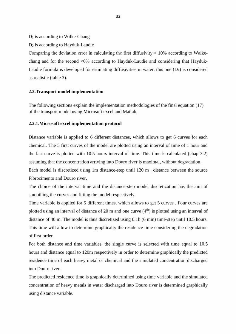
32
D1 is according to Wilke-Chang
D2 is according to Hayduk-Laudie
Comparing the deviation error in calculating the first diffusivity ≈ 10% according to Walke-
chang and for the second <6% according to Hayduk-Laudie and considering that Hayduk-
Laudie formula is developed for estimating diffusivities in water, this one (D2) is considered
as realistic (table 3).
2.2.Transport model implementation
The following sections explain the implementation methodologies of the final equation (17)
of the transport model using Microsoft excel and Matlab.
2.2.1.Microsoft excel implementation protocol
Distance variable is applied to 6 different distances, which allows to get 6 curves for each
chemical. The 5 first curves of the model are plotted using an interval of time of 1 hour and
the last curve is plotted with 10.5 hours interval of time. This time is calculated (chap 3.2)
assuming that the concentration arriving into Douro river is maximal, without degradation.
Each model is discretized using 1m distance-step until 120 m , distance between the source
Fibrocimento and Douro river.
The choice of the interval time and the distance-step model discretization has the aim of
smoothing the curves and fitting the model respectively.
Time variable is applied for 5 different times, which allows to get 5 curves . Four curves are
plotted using an interval of distance of 20 m and one curve (4th) is plotted using an interval of
distance of 40 m. The model is thus discretized using 0.1h (6 min) time-step until 10.5 hours.
This time will allow to determine graphically the residence time considering the degradation
of first order.
For both distance and time variables, the single curve is selected with time equal to 10.5
hours and distance equal to 120m respectively in order to determine graphically the predicted
residence time of each heavy metal or chemical and the simulated concentration discharged
into Douro river.
The predicted residence time is graphically determined using time variable and the simulated
concentration of heavy metals in water discharged into Douro river is determined graphically
using distance variable.

33
This concentration entering into Douro river is hence compared to the Limit Value of
Emission (LVE) of residues discharged into water given by the Decree-Law n° 236/98 of the
Ministry of Environment of Portugal.
2.2.2.Matlab implementation protocol
As for Microsoft excel, the interval of time of 0.1h (360sec) and the distance-step of 1m are
used to smooth and feet the curve and the model respectively, in matlab also, they are used
likewise but for time variable, the time is discretized until a value greater than 10.5h because
the simulated residence time is sometimes greater than that value. The protocols for both time
variable and distance variabl are given below.
2.2.2.1. Transport model-Time variable implementation protocol
% Transport model time evolution for each heavy metal/chemical;
% t is time in seconds;
% d is the distance in m;
% V is the velocity of water in m/sec;
% D is the diffusivity of each heavy metal/chemical in m2/sec;
% λ is the kinetic constant in 1/sec;
% Co is the initial concentration of each heavy metal/chemical in µg/l;
% C is the predicted concentration of heavy metal/chemical in µg/l;
clear
t=0:360:150000;
d=120;
D= value of diffisivity corresponding to each heavy metal/chemical;
V=0.003156;
λ= value of the kinetic constant corresponding to each heavy metal/chemical;
%A=sqrt(4×D×t);
%B=exp(-λ×t);
Co= initial value corresponding to each heavy metal/chemical;
if(d>(V×t)) ;
C=(Co/2)×erf((d-(t×V))/sqrt(4×D×t))×exp(-λ×t);
else
C=(Co/2)×(1+erf((t×V)-d)/sqrt(4×D×t))×exp(-λ×t);
end
plot(t,C)

34
2.2.2. 2.Transport model-Distance variable implementation protocol
% Transport model distance evolution for each heavy metal/chemical ;
% t is time in seconds;
% d is the distance in m,
% V is the velocity of water in m/sec;
% D is the diffusivity of each heavy metal/chemical in m2/sec;
% λ is the kinetic constant in 1/sec;
% Co is the initial concentration in µg/l;
% C is the predicted concentration of each heavy metal/chemical;
clear;
t=38013.27;
d=0:1:120;
D= value of diffisivity corresponding to each heavy metal/chemical;
V=0.003156;
λ= value kinetic constant corresponding to each heavy metal/chemical;
%A=sqrt(4×D×t);
%B=exp(-λ×t);
Co= initial value corresponding to each heavy metal/chemical;
if(d>(V×t)) ;
C=(Co/2)×erf((d-(t×V))/sqrt(4×D×t))×exp(-λ×t);
else
C=(Co/2)×(1+erf((t×V)-d)/sqrt(4×D×t))×exp(-λ×t);
end
plot(d,C)
2.3. Available data
2.3.1 Data from monitoring field
This method uses data from monitoring field made from 2007 until 2015. The following data
(table 4) are pH of water and concentration of heavy metals, other chemicals and sulfide at
different date. The data have been collected at the source of pollution (Fibrocimento tube), in
Douro river surface water and at 2.5 m deep.

35
Table 4: Concentration and pH of heavy metals and sulfide at Fibrocimento source, in Douro surface water and at 2.5m deep in water.
Date pH SO4 mg/L Al (μg/L) Cu (μg/L) Fe (μg/L) Mn (μg/L) Zn (μg/L) As (μg/L) Ni(μg/L) Pb (μg/L)
Source 27-08-2007 3.4 - - - - - - [17 - 19] [1.170 - 1.190] [4 - 5]
18-12-2008 3.1 - - - - - - [20 - 22] [1.400 - 1.420] [4 - 6]
24-08-2009 3.1 - - - - - - [3 - 4] [800 - 1000] [4 -5]
17-08-2010 3.2 - - - - - - [41 - 43] [1.220 - 1.240] [3 - 4]
18-10-2010 3.1 [1800 - 2000] - [60 - 70] [30500 - 30700 ] [150000 - 160000] [1400 - 1500] [50 - 70] [1.170 - 1.190] [3 - 4]
01-09-2011 3.2 [2100 - 2300] [21000 - 23000] [70 - 90] - - [1600 - 1800] - [1300 - 1400] -
11-01-2012 3.2 [1700 - 1900] [22000 - 24000] [60- 70] [44000 - 46000] [200000 - 220000] [1600 - 1800] [50 - 70] [1100 - 1300] -
28-08-2012 2.9 [1500 - 1700] [20000 - 22000] [80 - 90] [31000 - 33000] [2600 - 2800] [1400 - 1600] [11 - 13] [1100 - 1200] -
19-02-2013 3.8 [2100 - 2300] [20000 - 22000] [90 - 100] [112000 - 114000] [150000 - 170000] [1500 - 1700] [90 - 100] [1200 - 1300] -
27-08-2013 3.3 [1400 - 1600] [22000 - 24000] [50 - 70] [16000 - 18000] [130000 - 150000] [1300 - 1500] [30 - 40] [1100 - 1200] -
11-03-2014 5.4 [1800 - 2000] [1000 - 1200] [0.010 - 0.020] [90000 - 110000 ] [130000 - 150000] [1.1 - 1.3] [2 - 4] [900 - 1100] [2 - 4]
08-08-2014 3.8 [9 - 11] [4600 - 4800] [0.05 - 0.07] [1400- 1600] [6800 - 7000] [1.8 - 2.0] [2 - 4] [200 - 300] [0.002 - 0.003]
20-02-2015 4.7 [2000 - 2200] [2400 - 2600] [70- 90] [3200 - 3400] [6900 - 7100] [1400 - 1600] [900 - 100] [1200 - 1300] [0.002 - 0.003]
Douro surface
water
18-102010 7.5 [14 - 15] [11 - 13] [4 - 5] - - [10 - 12] [2 - 3] [3 - 4] [3 - 4]
11-01-2012 6.6 [23 - 25] [8 - 10] [4-6] [44000 - 46000] [200000 - 220000] [9 - 11] [3 - 5] [3 - 5] -
28-08-2013 7.7 [36 - 38] [10 - 12] [3 - 4] [91000 - 93000] [2600 - 2800] [12 - 14] [3 - 5] [3 - 5] -
19/02/2013 7.6 [15 - 17] [11 - 13] [3 - 5] [112000 - 114000] [150000 - 170000] [12 - 14] [2 - 4] [3 - 5] -
27/08/2013 8 [38 - 40] [12 - 14] [3 - 5] [16000 -18000] [130000 - 150000] [14 - 16] [3 - 5] [3 - 5] -
11/03/2014 8 [22 - 23] [7 - 9] [0.003 – 0.005 ] [90000 -110000] [130000 - 150000] [0.014 - 0.016] [2 - 4] [3 - 5] [3-5]
08/08/2014 7.4 [37-39] [29 - 31] [0.001 – 0.002] [1400 - 1600] [6800 - 7000] [0.04 - 0.06] [3 - 5] [0.004 - 0.006] [0.002 - 0.004]
20/02/2014 6.9 [21 - 23] [120 -140] [0.001 - 0.01] [3200 - 3400] [6900 -7100] [0.04 - 0.05] [0.002 - 0.003]
[0.004 - 0.005] [0.002 - 0.003]
Douro water
2.5m deep
18/10/2010 7.4 [14 - 15] [13 - 15] [4- 6] [9 - 11] [17 - 19] [10 - 12] [3 - 5] [3 - 4] [3 - 4]
11/03/2014 8 [21 - 22] [6 - 8] [0.003- 0.005] [45 - 47] [12 - 14] [0.014 - 0.016] [2 - 4] [3 - 5] [3- 5]
08/082014 7.5 [31 - 33] [20 - 40] [0.003- 0.005] [49 - 51] [0.014 - 0.016] [0.04 - 0.06] [2 - 4] [0.004 - 0.006] [0.002 - 0.004]
20/02/2015 7 [14 - 16] [120 - 140] [0.001- 0.01] [91 – 92 ] [36 - 38 ] [0.04 - 0.05] [0.002-0.003] [0.004 - 0.005] [0.002 - 0.003]

36
2.3.2. Calculated and converted dimensions
The table 5 shows existing dimensions, calculated and converted dimensions ( table 10 in
annexe) such as:
Section S (m2) of the pipe calculated using the measured diameter (0.55m) of the pipe;
Velocity V(m/s) of contaminated water exiting from the pipe, calculated using the following
formula: V = (24)
The dimension converted data is ( table 5):
Flow rate of contaminated water Q (l/s) converted from measured flow rate Q (l/min) exiting
from the pipe.
Table 5: Characteristic of the tube
Existing dimensions
Q exit the pipe (l/sec) 0.075
Diameter of Pipe (m) 0.550
Calculated dimensions
Section of Pipe (m2) 0.237
Velocity (m/s) 0.003

37
Chapter 3. RESULT AND DISCUSSION
3.1. Data analysis
When analyzing the given data from field monitorings made from 2007 to 2015, some
remarks appear:
The pH at the source of pollution, Fibrocimento tube is in the range of 2.9-5.4 and the pH in
Douro river is in the range of 6.6-8.0.
Some hypothetical assertions can be emitted:
The pH at the source of pollution, Fibrocimento, in the range of 2.9-5.4 is due to Acid Mine
Drainage (AMD) generation. But the river water has a pH in the buffer range of 6.6-8.0.
There should be occurred a natural attenuation of Acid Mine drainage.
There is an imminent risk of toxic pollution of heavy metals in Douro river.
Based on these hypothesis, this chapter is going to discuss the result and deliver a general and
realistic overview on the landfill coal ash pollution.
3.2. Results
Results depend on the assumed maximal time. The maximal time is the time calculated
assuming that the concentration of heavy metals or chemicals getting into Douro river is
maximal, without degradation or adsorption. This time is considered as maximal because it is
determined using the maximal distance of 120m.
With this assumption, in the equation 17; z = vt (25)
where z is the distance between Fibrocimento source of pollutants and Douro river, z = 120
m; and v is the velocity of water (m/sec), t is the time (sec).
t = (26)
As v = 3.15×10⁻³ m/sec, t = = 38013.27 sec, like 10.55 hours.
This time is applied in the model in order to get the predicted concentration of heavy metals
or chemicals discharged into Douro river considering degradation and adsorption.
The results for both excel and matlab implementation are presented with graphics of transport
model-time evolution and transport model-distance evolution (figures 9 to 56) and with table
6 and 7.

38
The result for matlab are presented to validate the result from Microsoft excel. For each
heavy metal or chemical, the graphic with one curve is ploted using time of 38013.27 sec
(10.5 h) for distance variable and 120m for time variable. From the transport model-time
variable, the smulated time residence is determined and from the transport model-distance
variable, the predicted concentration discharged into Douro river is determined like in excel
implementation.
3.2.1. Results from Microsoft excel implementation
3.2.1.1. Results from Microsoft excel for transport model-time evolution with
degradation from the source
One graphic with 5 curves and an other graphic with 1 curve explain the transport model-time
evolution for each heavy metal or chemical. In the graphic with 5 curves, the first curve C-
20m(µg/l) is plotted using a distance of 20 m from the source, the second curve C-40m(µg/l)
is plotted using 40 m from the source, the third curve C-60m(µg/l) is plotted using 60 m from
the source, the fourth curve C-100m(µg/l) is plotted using 100 m from the source and the fifth
curve C-120m(µg/l) is plotted using 120 m from the source ( distance between the source and
Douro river).
The choice of the number of plotted curves has the aim of smoothing and fitting the graphics.
It is not a determined and dependant number.
The fifth curve is hence extracted and constitute the second graphic with 1 curve. This
graphic allows to determine the residence time of every heavy metal or chemical in the area.
The following graphics explain the chemical’s behaviors from aluminum to lead.

39
Figure 9:Graphic of aluminum transport model- time evolution
This graphic (figure 9) describes the behavior of aluminum with the spread concentration at
the source of 23000 µg/l. The curve C-20m(µg/l) plotted with a distance of 20 m from the
source shows that the pick of maximal concentration occurs after 1 hour. The aluminum
maximal concentration is 5121.07 µg/l. This pick shows that even though there is a decrease
of concentration due to natural attenuation, there is an accumulation. From this pick, the
accumulation stops and starts the decreasing of accumulated chemical until a low
concentration of 0.00012 µg/l, after 35hours (smulated residence time). The second curve C-
40m(µg/l) plotted with a distance of 40 m from the source shows that the pick of maximal
concentration of 2638.73 µg/l occurs after 2 hours. The low concentration of 0.00012 µg/l
occurs at a simulated residence time of 35.2 hours. The third curve C-60m(µg/l) plotted with
a distance of 60 m from the source shows that the pick of maximal concentration of 1446.88
µg/l occurs after 2.7 hours. The low concentration of 0.00010 µg/l occurs at 35.6hours,
simulated residence time. The fourth curve C-100m(µg/l) plotted with 100m from the source
shows that the pick of maximal concentration of 463.25 µg/l occurs after 4 hours. The low
concentration of 0.00011 µg/l occurs at a simulated residence time of 35.4 hours. The fifth
curve C-120m(µg/l) is plotted with 120 m , distance from the source Fibrocimento to Douro
river ( figure 10)
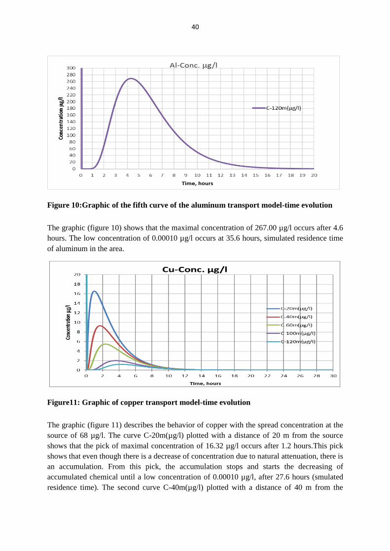
40
Figure 10:Graphic of the fifth curve of the aluminum transport model-time evolution
The graphic (figure 10) shows that the maximal concentration of 267.00 µg/l occurs after 4.6
hours. The low concentration of 0.00010 µg/l occurs at 35.6 hours, simulated residence time
of aluminum in the area.
Figure11: Graphic of copper transport model-time evolution
The graphic (figure 11) describes the behavior of copper with the spread concentration at the
source of 68 µg/l. The curve C-20m(µg/l) plotted with a distance of 20 m from the source
shows that the pick of maximal concentration of 16.32 µg/l occurs after 1.2 hours.This pick
shows that even though there is a decrease of concentration due to natural attenuation, there is
an accumulation. From this pick, the accumulation stops and starts the decreasing of
accumulated chemical until a low concentration of 0.00010 µg/l, after 27.6 hours (smulated
residence time). The second curve C-40m(µg/l) plotted with a distance of 40 m from the

41
source shows that the pick of maximal concentration of 9.11 µg/l occurs after 2 hours. The
low concentration of 0.00010 µg/l occurs at a simulated residence time of 27.6 hours. The
third curve C-60m(µg/l) plotted with a distance of 60 m from the source shows that the pick
of maximal concentration of 5.39 µg/l occurs after 2.6 hours. The low concentration of
0.00010 µg/l occurs at 27.6 hours which is the simulated residence time. The fourth curve C-
100m(µg/l) plotted with 100 m from the source shows that the pick of maximal concentration
of 1.98 µg/l occurs after 3.7 hours. The low concentration of 0.00010 (µg/l) occurs at a
simulated residence time of 27.6 hours. The fifth curve C-120m(µg/l) is plotted with 120 m ,
distance from the source Fibrocimento to Douro river ( figure 12).
Figure12: Graphic of the fith curve of copper transport model-time evolution
This graphic (figure 12) shows that the maximal concentration of 1.21 µg/l occurs after 4.3
hours. The low concentration of 0.00010 µg/l occurs at 27.5 hours, simulated residence time
of copper in the area.

42
Figure 13: Graphic of iron transport model-time evolution
The graphic (figure 13) describes the behavior of iron with the spread concentration at the
source of 45000 µg/l. The curve C-20m(µg/l) plotted with a distance of 20 m from the source
shows that the pick of maximal concentration of 14243.45 µg/l occurs after 2 hours.This pick
shows that even though there is a decrease of concentration due to natural attenuation, there is
an accumulation. From this pick, the accumulation stops and starts the decreasing of
accumulated chemical until a low concentration of 0.00010 µg/l, after 79 hours (smulated
residence time). The second curve C-40m(µg/l) plotted with a distance of 40 m from the
source shows that the pick of maximal concentration of 9671.59 µg/l occurs after 3 hours.
The low concentration of 0.00010 µg/l occurs at 79 hours. The third curve C-60m(µg/l)
plotted with a distance of 60 m from the source shows that the pick of maximal concentration
of 6699.71 µg/l occurs after 4.1 hours. The low concentration of 0.00010 µg/l occurs at 79
hours. The fourth curve C-100m(µg/l) plotted with 100 m from the source shows that the pick
of maximal concentration of 3357.96 µg/l occurs after 6.2 hours. The low concentration of
0.00010 µg/l occurs at 79 hours. The fifth curve C-120m(µg/l) is plotted with 120 m ,
distance from the source Fibrocimento to Douro river ( figure 14).

43
Figure 14: Graphic of the fith curve of iron transport model-time evolution
This graphic ( figure 14) shows that the maximal concentration of 2473.84 µg/l occurs after
6.8 hours. The low concentration of 0.00010 µg/l occurs at 79 hours, simulated residence
time of iron in the area.
Figure 15: Graphic of manganese transport model-time evolution
The graphic (figure 15) describes the behavior of manganese with the spread concentration at
the source of 210000 µg/l. The curve C-20m(µg/l) plotted with a distance of 20 m from the

44
source shows that the pick of maximal concentration of 58216.83 µg/l occurs after 1.3
hours.This pick shows that even though there is a decrease of concentration due to natural
attenuation, there is an accumulation. From this pick, the accumulation stops and starts the
decreasing of accumulated chemical until a low concentration of 0.00010 µg/l, after 59.5
hours (smulated residence time). The second curve C-40m(µg/l) plotted with a distance of 40
m from the source shows that the pick of maximal concentration of 35799.38 µg/l occurs
after 2.1 hours. The low concentration of 0.00010 µg/l occurs at 59.5 hours. The third curve
C-60m(µg/l) plotted with a distance of 60 m from the source shows that the pick of maximal
concentration of 22634.80 µg/l occurs after 3.1 hours. The low concentration of 0.00010 µg/l
occurs at 59.5 hours. The fourth curve C-100m(µg/l) plotted with 100 m from the source
shows that the pick of maximal concentration of 9699.67 µg/l occurs after 4.6 hours. The low
concentration of 0.00010 µg/l occurs at 59.5 hours. The fifth curve C-120m(µg/l) is plotted
with 120 m , distance from the source Fibrocimento to Douro river ( figure 16).
Figure 16: Graphic of the fith curve of manganese transport model-time evolution
This graphic ( figure 16) shows that the maximal concentration of 6422.03 µg/l occurs after
5.4 hours. The low concentration of 0.00010 µg/l occurs at 59.5 hours, simulated residence
time of manganese in the area.

45
Figure 17: Graphic of zinc transport model-time evolution
The graphic (figure 17) describes the behavior of zinc with the spread concentration at the
source of 1700 µg/l. The curve C-20m (µg/l) plotted with a distance of 20 m from the source
shows that the pick of maximal concentration of 391.08 µg/l occurs after 1.2 hours.This pick
shows that even though there is a decrease of concentration due to natural attenuation, there is
an accumulation. From this pick, the accumulation stops and starts the decreasing of
accumulated chemical until a low concentration of 0.00010 µg/l, after 32.7 hours (smulated
residence time). The second curve C-40m(µg/l) plotted with a distance of 40 m from the
source shows that the pick of maximal concentration of 210.26 µg/l occurs after 2 hours. The
low concentration of 0.00010 µg/l occurs at 32.7 hours. The third curve C-60m(µg/l) plotted
with a distance of 60 m from the source shows that the pick of maximal concentration of
118.77 µg/l occurs after 2.7 hours. The low concentration of 0.00010 µg/l occurs at 32.7
hours. The fourth curve C-100m(µg/l) plotted with 100 m from the source shows that the pick
of maximal concentration of 40.27 µg/l occurs after 4 hours. The low concentration of
0.00010 µg/l occurs at 32.7 hours. The fifth curve C-120m(µg/l) is plotted with 120 m ,
distance from the source Fibrocimento to Douro river ( figure 18).

46
Figure 18: Graphic of the fith curve of zinc transport model-time evolution
This graphic ( figure 18) shows that the maximal concentration of 23.73 µg/l occurs after 4.7
hours. The low concentration of 0.00010 µg/l occurs at 32.6 hours, simulated residence time
of zinc in the area.
Figure 19: Graphic of arsenic transport model-time evolution
The graphic (figure 19) describes the behavior of arsenic with the spread concentration at the
source of 60 µg/l. The curve C-20m (µg/l) plotted with a distance of 20 m from the source
shows that the pick of maximal concentration of 10.91 µg/l occurs after 1 hour.This pick
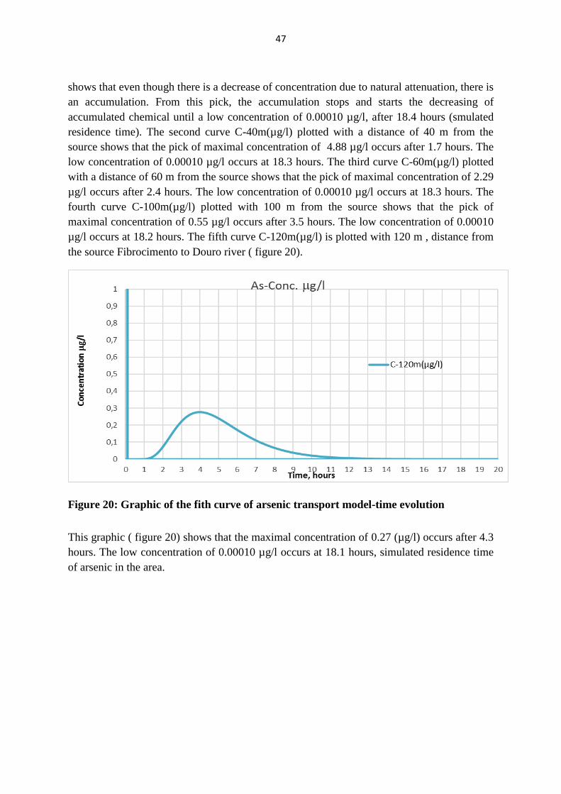
47
shows that even though there is a decrease of concentration due to natural attenuation, there is
an accumulation. From this pick, the accumulation stops and starts the decreasing of
accumulated chemical until a low concentration of 0.00010 µg/l, after 18.4 hours (smulated
residence time). The second curve C-40m(µg/l) plotted with a distance of 40 m from the
source shows that the pick of maximal concentration of 4.88 µg/l occurs after 1.7 hours. The
low concentration of 0.00010 µg/l occurs at 18.3 hours. The third curve C-60m(µg/l) plotted
with a distance of 60 m from the source shows that the pick of maximal concentration of 2.29
µg/l occurs after 2.4 hours. The low concentration of 0.00010 µg/l occurs at 18.3 hours. The
fourth curve C-100m(µg/l) plotted with 100 m from the source shows that the pick of
maximal concentration of 0.55 µg/l occurs after 3.5 hours. The low concentration of 0.00010
µg/l occurs at 18.2 hours. The fifth curve C-120m(µg/l) is plotted with 120 m , distance from
the source Fibrocimento to Douro river ( figure 20).
Figure 20: Graphic of the fith curve of arsenic transport model-time evolution
This graphic ( figure 20) shows that the maximal concentration of 0.27 (µg/l) occurs after 4.3
hours. The low concentration of 0.00010 µg/l occurs at 18.1 hours, simulated residence time
of arsenic in the area.

48
Figure 21: Graphic of nickel transport model-time evolution
The graphic (figure 21) describes the behavior of nickel with the spread concentration at the
source of 1200 µg/l. The curve C-20m(µg/l) plotted with a distance of 20 m from the source
shows that the pick of maximal concentration of 433.82 µg/l occurs after 2.4 hours.This pick
shows that even though there is a decrease of concentration due to natural attenuation, there is
an accumulation. From this pick, the accumulation stops and starts the decreasing of
accumulated chemical until a low concentration of 0.00010 µg/l, after 90.5 hours (smulated
residence time). The second curve C-40m(µg/l) plotted with a distance of 40 m from the
source shows that the pick of maximal concentration of 319.52 µg/l occurs after 3.4 hours.
The low concentration of 0.00010 µg/l occurs at 90.4 hours. The third curve C-60m(µg/l)
plotted with a distance of 60 m from the source shows that the pick of maximal concentration
of 239.25 µg/l occurs after 4.6 hours. The low concentration of 0.00010 µg/l occurs at 90.4
hours. The fourth curve C-100m(µg/l) plotted with 100 m from the source shows that the pick
of maximal concentration of 140.27 µg/l occurs after 6.6 hours. The low concentration of
0.00010 µg/l occurs at 90.4 hours. The fifth curve C-120m(µg/l) is plotted with 120 m ,
distance from the source Fibrocimento to Douro river ( figure 22).

49
Figure 22 : Graphic of the fith curve of nickel transport model-time evolution
This graphic ( figure 22) shows that the maximal concentration of 107 µg/l occurs after 4.3
hours. The low concentration of 0.00010 µg/l occurs at 90.4 hours, simulated residence time
of nickel in the area.
Figure 23: Graphic of lead transport model-time evolution
The graphic (figure 23) describes the behavior of lead with the spread concentration at the
source of 3 µg/l. The curve C-20m(µg/l) plotted with a distance of 20 m from the source
shows that the pick of maximal concentration of 0.24 µg/l occurs after 0.6 hour.This pick
shows that even though there is a decrease of concentration due to natural attenuation, there is

50
an accumulation. From this pick, the accumulation stops and starts the decreasing of
accumulated chemical until a low concentration of 0.00010 µg/l, after 5.6 hours (smulated
residence time). The second curve C-40m(µg/l) plotted with a distance of 40 m from the
source shows that the pick of maximal concentration of 0.058 µg/l occurs after 1.1 hours.
The low concentration of 0.00010 µg/l occurs at 5.5 hours. The third curve C-60m(µg/l)
plotted with a distance of 60 m from the source shows that the pick of maximal concentration
of 0.015 µg/l occurs after 1.5 hours. The low concentration of 0.00010 µg/l occurs at 5.3
hours. The fourth curve C-100m(µg/l) plotted with 100 m from the source shows that the pick
of maximal concentration of 0.004 µg/l occurs after 1.9 hours. The low concentration of
0.00010 µg/l occurs at 5.1 hours. The fifth curve C-120m(µg/l) is plotted with 120 m ,
distance from the source Fibrocimento to Douro river ( figure 24).
Figure 24: Graphic of the fith curve of lead transport model-time evolution
This graphic ( figure 24) shows that the maximal concentration of 0.00029 µg/l occurs after
2.8 hours. The low concentration of 0.00010 µg/l occurs at 4.3 hours, simulated residence
time of lead in the area.
3.2.1.2.Results from Microsoft excel for transport model- distance evolution with
degredation fromthe source
Like in the transport model-time evolution, two type of graphics explain the transport model.
One graphic has one curve and another one has six curves, the first curve C-1h(µg/l) is
plotted with time from the start equal to 1 hour (3600sec), the second curve C-2h(µg/l) is
plotted with the time from the start equal to 2 hours (7200sec), the third curve C-3h(µg/l) is

51
plotted with the time from the start equal to 3 hours (10800 sec), the fourth curve C-4h(µg/l)
is plotted with the time from the start equal to 4 hors (14400 sec), the fifth curve C-5h(µg/l) is
plotted with the time from the start equal to 5 hours (18000 Sec), the sixth curve C-
10.5h(µg/l) is plotted with the time from the start equal to 10.5 hours (38013.27 sec).
Also in this case, the choice of the number of plotted curves has the aim of smoothing and
fitting the graphics, it is not a determined and dependant number.
The sixth curve is selected and constitute the second type of graphic with one curve. This
graphic allows to determine the simulated concentration discharged into Douro river.
Figure 25: Graphic of aluminum transport model-distance evolution
The graphic (figure 25) describes the behavior of aluminum in the transport model-distance
evolution with the spread concentration of 23000 µg/l at the source. The curve C-1h(µg/l)
plotted with a time of 1 hour from the start shows that the concentration of aluminum in
water discharged into Douro river after 1 hour is equal to 1.07 µg/l . The second curve C-
2h(µg/l) plotted with a time of 2 hours from the start shows that the concentration of
aluminum in water discharged into Douro river is 6.54.101 µg/l. The third curve C-3h(µg/l)
plotted with a time of 3 hours from the start shows that the concentration of aluminum in
water is 1.92.102 µg/l. The fourth curve C-4h(µg/l) plotted with time of 4 hours from the start
shows that the concentration of aluminum in water is 2.58.102 µg/l. The fifth curve C-

52
5h(µg/l) plotted with a time of 5 hours from the start shows that the concentration of
aluminum in water is 2.51.102 µg/l. With the sixth curve, the predicted concentration of
aluminum in water discharded into Douro river is determined by figure 26.
Figure 26: Graphic of the sixth curve of aluminum transport model-distance evolution
This graphic (figure 26) determines that the predicted concentration of aluminum in water
discharged into Douro river is 3.89.101 µg/l.
Figure 27: Graphic of copper transport model- distance evolution
The graphic (figure 27) describes the behavior of copper in the transport model-distance
evolution with the spread concentration of 68 µg/l at the source. The curve C-1h(µg/l) plotted

53
with a time of 1 hour from the start shows that the concentration of copper in water
discharged into Douro river after 1 hour is equal to 1.49.10-2 µg/l . The second curve C-
2h(µg/l) plotted with a time of 2 hours from the start shows that the concentration of copper
in water is 4.15.10-1 µg/l. The third curve C-3h(µg/l) plotted with a time of 3 hours from the
start shows that the concentration of copper in water is 9.77.10-1 µg/l. The fourth curve C-
4h(µg/l) plotted with a time of 4 hours from the start shows that the concentration of copper
in water is 1.18 µg/l. The fifth curve C-5h(µg/l) plotted with a time of 5 hours from the start
shows that the concentration of copper in water is 2.05.10-1 µg/l. With the sixth curve, the
predicted concentration of copper in water discharded into Douro river is determined by the
figure 28.
Figure 28: Graphic of the sixth curve of copper transport model-distance evolution
This graphic (figure 28) determines that the predicted concentration of copper in water
discharged into Douro river is 2.05.10-1 µg/l.

54
Figure 29: Graphic of iron transport model-distance evolution
The graphic (figure 29) describes the behavior of iron in the transport model- distance
evolution with the spread concentration of 45000 µg/l at the source. The curve C-1h(µg/l)
plotted with a time of 1 hour from the start shows that the concentration of iron in water
discharged into Douro river after 1 hour is equal to 1.26.101 µg/l . The second curve C-
2h(µg/l) plotted with a time of 2 hours from the start shows that the concentration of iron in
water is 4.15.102 µg/l. The third curve C-3h(µg/l) plotted with a time of 3 hours from the start
shows that the concentration of iron in water is 1.30.103 µg/l. The fourth curve C-4h(µg/l)
plotted with a time of 4 hours from the start shows that the concentration of iron in water is
1.97.103 µg/l. The fifth curve C-5h(µg/l) plotted with a time of 5 hours from the start shows
that the concentration of iron in water is 2.42.103 µg/l. With the sixth curve, the predicted
concentration of iron in water discharded into Douro river is determined by the figure 30.

55
Figure 30: Graphic of the sixth curve of iron transport model-distance evolution
This graphic (figure 30) determines that the predicted concentration of iron in water
discharged into Douro river is 1.57.103 µg/l.
Figure 31: Graphic of manganese transport model-distance evolution
The graphic (figure 31) describes the behavior of manganese in the transport model- distance
evolution with the spread concentration of 210000 µg/l at the source. The curve C-1h(µg/l)
plotted with a time of 1 hour from the start shows that the concentration of manganese in
water discharged into Douro river after 1 hour is equal to 4.63.101 µg/l. The second curve C-
2h(µg/l) plotted with a time of 2 hours from the start shows that the concentration of
manganese in water is 1.56.103 µg/l. The third curve C-3h(µg/l) plotted with a time of 3
hours from the start shows that the concentration of manganese in water is 4.23.103 µg/l.

56
The fourth curve C-4h(µg/l) plotted with time of 4 hours from the start shows that the
concentration of manganese in water is 5.84.103 µg/l. The fifth curve C-5h(µg/l) plotted with
a time of 5 hours from the start shows that the concentration of manganese in water is
6.49.103 µg/l. With the sixth curve, the predicted concentration of manganese in water
discharded into Douro river is determined by the figure 32.
Figure 32: Graphic of the sixth curve of manganese transport model-distance evolution
This graphic (figure 32) determines that the predicted concentration of manganese in water
discharged into Douro river is 2.35.103 µg/l.
Figure 33: Graphic of zinc transport model-Distance evolution

57
The graphic (figure 33) describes the behavior of zinc in the transport model- distance
evolution with the spread concentration of 1700 µg/l at the source. The curve C-1h(µg/l)
plotted with a time of 1 hour from the start shows that the concentration of zinc in water
discharged into Douro river after 1 hour is equal to 1.36.101 µg/l . The second curve C-
2h(µg/l) plotted with a time of 2 hours from the start shows that the concentration of zinc in
water is 6.47 µg/l. The third curve C-3h(µg/l) plotted with a time of 3 hours from the start
shows that the concentration of zinc in water is 1.78.101 µg/l. The fourth curve C-4h(µg/l)
plotted with a time of 4 hours from the start shows that the concentration of zinc in water is
2.29.101 µg/l. The fifth curve C-5h(µg/l) plotted with a time of 5 hours from the start shows
that the concentration of zinc in water is 3.31.101 µg/l. With the sixth curve, the predicted
concentration of zinc in water discharded into Douro river is determined by the figure 34.
Figure 34: Graphic of the sixth curve of zinc transport model-distance evolution
This graphic (figure 34) determines that the predicted concentration of zinc in water
discharged into Douro river is 4.02 µg/l.

58
Figure 35: Graphic of arsenic transport model-Distance evolution
The graphic (figure 35) describes the behavior of arsenic in the transport model-distance
evolution with the spread concentration of 60 µg/l at the source. The curve C-1h(µg/l) plotted
with a time of 1 hour from the start shows that the concentration of arsenic in water
discharged into Douro river after 1 hour is equal to 6.39.10-4 µg/l. The second curve C-
2h(µg/l) plotted with a time of 2 hours from the start shows that the concentration of arsenic
in water is 6.82.10-2 µg/l. The third curve C-3h(µg/l) plotted with a time of 3 hours from the
start shows that the concentration of arsenic in water is 2.13.10-1 µg/l. The fourth curve C-
4h(µg/l) plotted with time of 4 hours from the start shows that the concentration of arsenic in
water is 2.68.10-1 µg/l. The fifth curve C-5h(µg/l) plotted with a time of 5 hours from the start
shows that the concentration of arsenic in water is 2.33.10-1 µg/l. With the sixth curve, the
predicted concentration of arsenic in water discharded into Douro river is determined by the
figure 36.

59
Figure 36: Graphic of the sixth curve of arsenic transport model-distance evolution
This graphic (figure 36) determines that the predicted concentration of arsenic in water
discharged into Douro river is 1.50.10-2 µg/l.
Figure 37: Graphic of nickel transport model-distance evolution
The graphic (figure 37) describes the behavior of nickel in the transport model-distance
evolution with the spread concentration of 1200 µg/l at the source. The curve C-1h(µg/l)
plotted with a time of 1 hour from the start shows that the concentration of nickel in water
discharged into Douro river after 1 hour is equal to 4.69.10-1 µg/l. The second curve C-
2h(µg/l) plotted with a time of 2 hours from the start shows that the concentration of nickel

60
in water is 1.51.101 µg/l. The third curve C-3h(µg/l) plotted with a time of 3 hours from the
start shows that the concentration of nickel in water is 4.58.101 µg/l. The fourth curve C-
4h(µg/l) plotted with time of 4 hours from the start shows that the concentration of nickel in
water is 7.30.101 µg/l. The fifth curve C-5h(µg/l) plotted with a time of 5 hours from the start
shows that the concentration of nickel in water is 9.50.101 µg/l. With the sixth curve, the
predicted concentration of nickel in water discharded into Douro river is determined by the
figure 38.
Figure 38: Graphic of the sixth curve of nickel transport model-distance evolution
This graphic (figure 38) determines that the predicted concentration of nickel in water
discharged into Douro river is 8.97.101 µg/l.
Figure 39: Graphic of lead transport model-distance evolution
The graphic (figure 39) describes the behavior of lead in the transport model-distance
evolution with the spread concentration of 3 µg/l at the source. The curve C-1h(µg/l) plotted

61
with a time of 1 hour from the start shows that the concentration of lead in water discharged
into Douro river after 1 hour is equal to 1.97.10-6 µg/l . The second curve C-2h(µg/l) plotted
with a time of 2 hours from the start shows that the concentration of lead in water is 1.94.10-4
µg/l. The third curve C-3h(µg/l) plotted with a time of 3 hours from the start shows that the
concentration of lead in water is 2.85.10-4 µg/l. The fourth curve C-4h(µg/l) plotted with a
time of 4 hours from the start shows that the concentration of lead in water is 1.44.10-4 µg/l.
The fifth curve C-5h(µg/l) plotted with a time of 5 hours from the start shows that the
concentration of lead in water is 4.68.10-5 µg/l. With the sixth curve, the predicted
concentration of lead in water discharded into Douro river is determined by the figure 40.
Figure 40: Graphic of the sixth curve of lead transport model-Distance evolution
This graphic (figure 40) determines that the predicted concentration of lead in water
discharged into Douro river is 8.89.10-9 µg/l.
The following table 6 shows the simulated residence time of each chemical in the area and
the predicted concentration discharged into Douro river from Microsoft excel
implementation.

62
Table 6: Simulated residence time and predicted values of concentration from excel
implementation of each chemical getting into Douro river
Element Simulated residence
time (hours)
Predicted values of
concentration
discharged into
Douro river (µg/l)
Predicted values of
concentration
discharged into
Douro river (mg/l)
Al 35.6 3.8 ×101 3.8×10⁻²
Cu 27.5 2.0×10⁻¹ 2.0×10⁻⁴
Fe 79 1.5×10³ 1.5
Mn 59.5 2.3×10³ 2.3
Zn 32.6 4.0 4.0×10⁻³
As 18.1 1.5×10⁻² 1.5×10⁻⁵
Ni 90.4 8.9×101 8.9×10⁻²
Pb 4.3 8.8×10⁻⁹ 8.8×10⁻¹²
3.2.2. Results from matlab implementation
In this section the graphics of one curve are presented with the corresponding variables as
defined in the protocol implementation methodology (section 2.2.2.) to determine the
simulated residence time and the predicted concentration of heavy metals or other chemicals
decharged into Douro river.

63
3.2.2.1. Matlab results for a transport model- time evolution with degradation from the
source
The following graphics are ploted for all heavy metals and other chemicals.
Figure 41: Aluminum transport model-time evolution graphic from matlab
Aluminum low concentration of 0.00010 µg/l occurs at 124560 sec (34.6 h), smulated
residence time.
Figure 42: Iron transport model-time evolution graphic from matlab
Iron low concentration of 0.00010 µg/l occurs at 274680 sec (76.3 h), simulated residence
time.

64
Figure 43: Copper transport model-time evolution graphic from matlab
Copper low concentration of 0.00010 µg/l occurs at 95040 sec (26.4 h), simulated residence
time.
Figure 44: Manganese transport model-time evolution graphic from matlab
Manganese low concentration of 0.00010 µg/l occurs at 207720 sec ( 57.7h), simulated
residence time.

65
Figure 45: Zinc transport model-time evolution graphic from matlab
Zinc low concentration of 0.00010 µg/l occurs at 113760 sec ( 31.6 h), simulated residence
time.
Figure 46: Arsenic transport model-time evolution graphic from matlab
Arsenic low concentration of 0.00010 µg/l occurs at 63000sec ( 17.5 h), simulated residence
time.

66
Figure 47: Nickel transport model-time evolution graphic from matlab
Nickel low concentration of 0.00010 µg/l occurs at 312120 sec ( 86.7 h), simulated residence
time.
Figure 48: Lead transport model-time evolution graphic from matlab
Lead low concentration of 0.00010 µg/l occurs at 18360 sec ( 5.1 h), simulated residence
time.
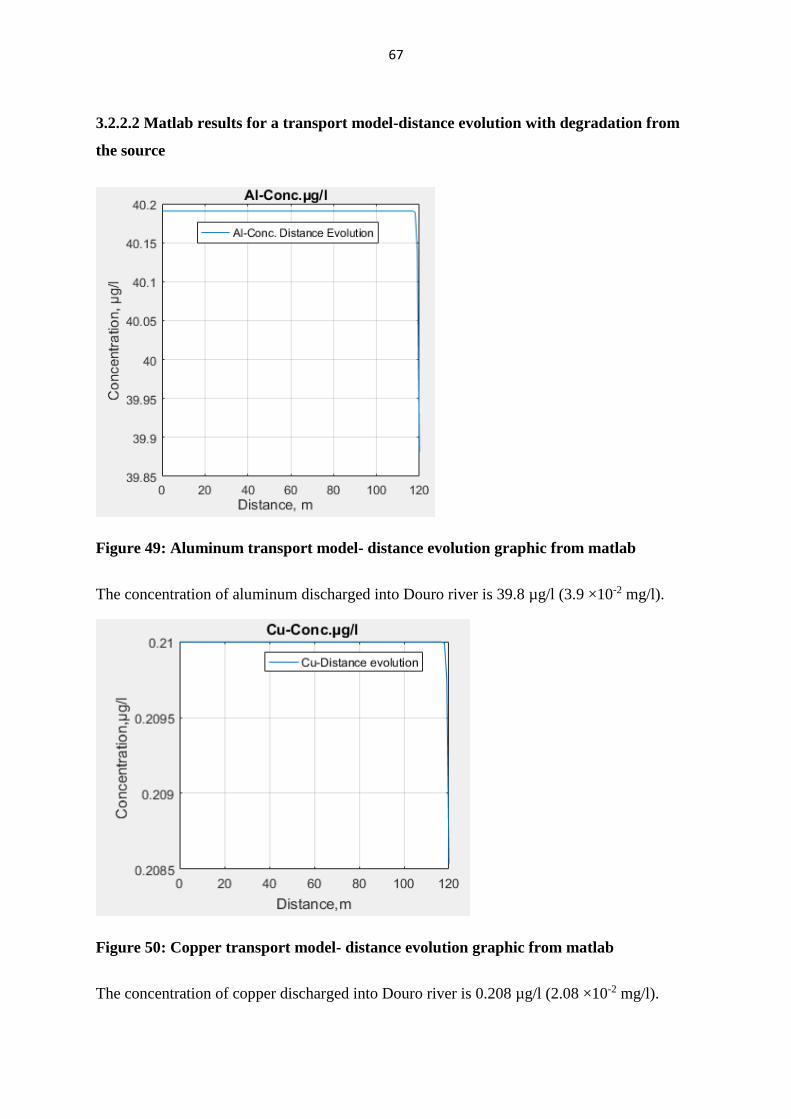
67
3.2.2.2 Matlab results for a transport model-distance evolution with degradation from
the source
Figure 49: Aluminum transport model- distance evolution graphic from matlab
The concentration of aluminum discharged into Douro river is 39.8 µg/l (3.9 ×10⁻² mg/l).
Figure 50: Copper transport model- distance evolution graphic from matlab
The concentration of copper discharged into Douro river is 0.208 µg/l (2.08 ×10⁻² mg/l).

68
Figure 51: Iron transport model- distance evolution graphic from matlab
The concentration of iron discharged into Douro river is 1.57×10³ µg/l (1.57 mg/l).
Figure 52: Manganese transport model- distance evolution graphic from matlab
The concentration of manganese discharged into Douro river is 2.34×10³ µg/l (2.34 mg/l).

69
Figure 53: Zinc transport model- distance evolution graphic from matlab
The concentration of zinc discharged into Douro river is 4.15 µg/l (4.15×10⁻³ mg/l).
Figure 54: Arsenic transport model- distance evolution graphic from matlab
The concentration of arsenic discharged into Douro river is 1.51×10⁻² µg/l (1.51×10⁻⁵ mg/l).

70
Figure 55: Nickel transport model- distance evolution graphic from matlab
The concentration of nickel discharged into Douro river is 89.6 µg/l (8.9×10⁻² mg/l).
Figure 56: Lead transport model- distance evolution graphic from matlab
The concentration of lead discharged into Douro river is 9.00×10⁻⁹ µg/l (9.00×10⁻¹² mg/l).
The following table7, presents the results from matlab of predicted concentration discharged
into Douro and the simulated residence time of each heavy metal or other chemical.

71
Table 7: Simulated residence time and predicted values of concentration of heavy
metals and other chemicals discharged into Douro river from matlab implementation
Element Simulated residence
time from Matlab
(hours)
Predicted values of
concentration
discharged into Douro
river from Matlab
(mg/l)
Al 34.6 3.9×10⁻²
Cu 26.4 2.0×10⁻²
Fe 76.3 1.5
Mn 57.7 2.3
Zn 31.6 4.1
As 17.5 1.5×10⁻⁵
Ni 86.7 8.9×10⁻²
Pb 5.1 9.0×10⁻¹²
3.3.Microsoft-Excel and matlab cross validation
In this section a cross validation is made by comparison of values from excel and matlab (
table 8).The comparison shows that there is not a very great variation in values, the low
difference between some values could be due to instrumental error. Every one could consider
to use the result from Matlab or from Microsoft-excel, there is no change concerning the
conclusion.
In the following sections, the values from Microsoft-excel are used in the comparison with
the threshold limit values.

72
Table 8: Excel and Matlab cross validation values
Element Simulated
residence time
from Excel
(hours)
Predicted values
of concentration
discharged into
Douro river from
Excel (mg/l)
Simulated
residence time
from Matlab
(hours)
Predicted values
of concentration
discharged into
Douro river from
Matlab (mg/l)
Al 35.6 3.8×10⁻² 34.6 3.9×10⁻²
Cu 27.5 2.0×10⁻⁴ 26.4 2.0×10⁻²
Fe 79 1.5 76.3 1.5
Mn 59.5 2.3 57.7 2.3
Zn 32.6 4.0×10⁻³ 31.6 4.1
As 18.1 1.5×10⁻⁵ 17.5 1.5×10⁻⁵
Ni 90.4 8.9×10⁻² 86.7 8.9×10⁻²
Pb 4.3 8.8×10⁻¹² 5.1 9.0×10⁻¹²
3.4. Discussion
Based on the two hypotheses formulated previously in section 3.1., this section discusses how
is the evolution of the pollution of water from the landfill coal ash to Douro river. This
pollution could occur in two possible ways:
1. Toxicity caused by the concentration of heavy metals or other chemicals in water
discharged into Douro river;
2. Acidity of water caused by the AMD of water discharged into Douro river.
3.4.1. Toxicity caused by the concentration of heavy metals in water
The analyse of the evolution of the concentration of heavy metals or other chemicals in water
from the landfill coal ash to Douro river and the comparison (Table 9) of the concentration of
heavy metals or other chemicals in water discharged into Douro river to the threshold limit
value of emission of residues in water, shows that only manganese exceeds the threshold
limit value according to data collected in the monitoring field on 11th January, 2012 . During

73
the previous and followed monitoring field, the concentration measured at the source was
lower, which means manganese is not an acute environemental threat. The concentrations of
other heavy metals or chemicals do not exceed the threshold limit value. All of them are
degraded in the pathway to Douro river.
This shows that heavy metals or chemicals are removed from polluted water when it is
flowing through soils from the source Fibrocimento to Douro river. This is a natural
attenuation, the way how it occurs is explained in the section 3.4.3.
Table 9: Comparison of predicted values of concentration discharged into Douro river
to the threshold limit values
Heavy metal element Predicted values of
concentration discharged into
Douro river (mg/l)
Threshold limit
values (mg/l)
Al 3.8×10⁻² 10
Cu 2.0×10⁻⁴ 1.0
Fe 1.5 2.0
Mn 2.3 2.0
Zn 4.0×10⁻³ 0.5
AS 1.5×10⁻⁵ 1.0
Ni 8.9×10⁻² 2.0
Pb 8.8×10⁻¹² 1.0
3.4.2.Acidity of water caused by the AMD
The analyse of pH of water at the source in the range of 2.9-5.4 reveals that AMD is occured.
But the pH 6.6-8.0 of water in Douro river is in the buffer range. This shows that a natural
attenuation of AMD and pH buffering occurred during the path way from the source to Douro
river. This natural attenuation of AMD and pH buffering is explained in the section 3.4.4.

74
3.4.3. Natural attenuation of heavy metals
From Fibrocimento pipe to Douro river, polluted water is flowing on surface ground and
through soils. There is an interaction between soil and water and soil composition is playing a
key role in natural attenuation as a filter. Clay minerals have a great potentiality to adsorb
heavy metals due to their large specific surface area, chemical and mechanical stability,
layered structure, and high cationic exchanger capacity (Sdiri et al., 2011). Natural organic
compounds in the soil plays also a key role of heavy metals and other chemicals attenuation
by adsorption (Badawi et al., 2017, Assis & Valmir, 2003). Those materials playing a role of
natural attenuation are assumed to be occurring in the study area.
3.4.4.Natural attenuation of AMD and pH buffering
Natural attenuation of acidity and pH buffering turn out to be a critical control on the
environmental behavior.
As acidity is released to solution during pyrite weathering, the pH drops. There are other
minerals however, that can consume acidity as they dissolve, thereby producing natural
attenuation of acidity produced by pyrite weathering, helping to buffer the pH (Younger et
al., 2002).
The natural attenuation of AMD occurs in two phases, by primary minerals weathering and
by authigenic secondary minerals formation.
The first phase implys primary minerals of rock fragments, and as this case study deals with
surface water flowing on surface ground , this phase is not applicable.
The second phase is applicable as it implys solutions and dissolved minerals. This
phenomenon is explained in the following section.
3.4.4. 1.Authigenic secondary minerals formation
Secondary minerals are formed through precipitation from contaminated solutions. They are
within sediments and occur as a coating on surfaces of mineralized clasts where they partially
or completely replace them (Carbone et al., 2013).
The characteristic of secondary minerals formed during AMD depend on variation in
chemical conditions of the receiving environment (particularly variation in pH, Eh, and
temperature).

75
From a genetic point of view, three main settings for secondary mineral formation can be
distinguished:
1. Unconsolidated precipitates, flocs, and lose suspensions;
2. Consolidated crusts and hardpans precipitating from seepage drainage of
contaminated solutions within waste-rock dumps and tailings;
3. Efflorescent salts formed mainly on the surface waste rock deposits, tailing, and mine
soils due to evaporation of mine waters in dry periods or as a consequence of the heat
produced by exothermic reactions active during sulphide oxidation (Carbone et al.,
2013).
As this case study deals with polluted water, the first setting formation of secondary minerals
has a realistic meaningful explanation.
Even the mineralogy of the formed secondary minerals is quite variable, the main minerals
can be grouped into three broad groups:
Fe-oxides, oxydroxides, and oxyhydroxysulphates (such as ferrihydrites 2), goethite,
hematite, schwertmanite and jarosite, and other low crystalline Fe phases;
Hydrous Ca, Fe, Al, and other metal sulphates (such as gypsum, melanterite, copiapite,
halotrichite, chalcanthite, and episomite);
Other metal rich phases, usually with low crystalline, are basaluminite like Al minerals,
woodwardite like Cu minerals and hydrozincite.
All these minerals have specific fields of stability within the wide range of pH and Eh
conditions that typically occur in AMD environment (Carbone et al., 2013).

76
Chapter 4 : CONCLUSION AND RECOMMENDATIONS
4.1. Conclusion
This work “Water contamination in the area of a landfill coal ash” conducted by
implementing the transport model of height chemicals in water contaminated by the leachate
coming from the landfill coal ash in the area of Medas, Municipality of Gondomar, nearby
Douro river reveals that the landfill coal ash is not a very big problematic pollution of Douro
river.
Based on the transport model development using the Fickian first law and the implementation
of the model using Microsoft excel and matlab, the results show that the concentration of
only 1 chemical, Manganese in water discharged into Douro river exceeds the threshold limit
value allowed by the Ministry of Environment of Portugal. This is not an imminent pollution
threat as the applied concentration in the model was measured during the monitoring field
made on 11/01/2012. This high value occurred once time. During the previous and followed
monitoring fields, the measured concentration had low values than the used one.
The decrease of concentration of heavy metals during the pathway from Fibrocimento to
Douro river is due to natural attenuation by adsorption of natural clay minerals and sorption
into organic matter of the soil in the area.
Based on the analysis of AMD, causes and manifestations, there is also a natural attenuation
occurring due to authigenic secondary minerals occurring during AMD itself.
4.2. Recommendations for future works
For future works, I recommend to environmental researchers to:
Make a field sample of soil along the water path in order to analyze the soil density ρ;
soil-water partition coefficient Ks; organic-carbon partition coefficient Kco; organic
material fraction fco and octanol-water partition coefficient Kwo. All those
parameters can help to calculate the retardation coefficient which can hence end up to
getting the biodegradation kinetic constant;
Undertake experimental studies concerning how a natural attenuation of heavy metals
occurs by using natural minerals along the fibrocimento-Douro river pathway;
Undertake experimental studies concerning how natural attenuation of AMD and pH
buffering happens along the fibrocimeto-Douro river pathway.

77
References
Acreman, M. (2004). Water and Ecology. Series on Water and Ethics (World
Comm, Vol. 8). Paris: UNESCO.
Aderinola, O. J., Clarke, E. O., Olarinmoye, O. M., Kusemiju, V., & Anatekhai,
M. A. (2012). Heavy Metals in Surface Water, Sediments, Fish and
Perwinkles of Lagos Lagoon. Journal Of Agricultural & Environmental
Sciences, 5(5), 609–617.
Assis, O. B. G., & Valmir, L. da S. (2003). Caracterização estrutural e da
capacidade de absorção de água em filmes finos de quitosana processados
em diversas concentrações. Polímeros, 13(4), 223–228.
http://doi.org/10.1590/S0104-14282003000400006
Authman, M. M. N., Zaki, M. S., Khallaf, E. A., & Abbas, H. H. (2015). Use of
Fish as Bio-indicator of the Effects of Heavy Metals Pollution. Aquaculture
Research & Development, 6(4). http://doi.org/10.4172/2155-9546.1000328
Badawi, M. A., Negm, N. A., Abou Kana, M. T. H., Hefni, H. H., & Abdel
Moneem, M. M. (2017). Adsorption of aluminum and lead from wastewater
by chitosan-tannic acid modified biopolymers: Isotherms, kinetics,
thermodynamics and process mechanism. International Journal of
Biological Macromolecules, 99, 465–476.
http://doi.org/10.1016/j.ijbiomac.2017.03.003
Badiye, A., Kapoor, N., & Khajuria, H. (2013). Copper Toxicity : A
Comprehensive Study. Research Journal of Recent Sciences, 2, 58–67.
Retrieved from www.isca.in
Batu, V. (2006). Applied flow and solute transport modeling in aquifers:
fundamental principals and analytical and numerical methods. (Taylor &
Francis, Eds.)Textbook (CRC Press). U. S.A. Retrieved from

78
http://www.crcpress.com
Carbone, C., Dinelli, E., Marescotti, P., Gasparotto, G., & Lucchetti, G. (2013).
The role of AMD secondary minerals in controlling environmental
pollution: Indications from bulk leaching tests. Journal of Geochemical
Exploration, 132, 188–200. http://doi.org/10.1016/j.gexplo.2013.07.001
Carolin, C. F., Kumar, P. S., Saravanan, A., Joshiba, G. J., & Naushad, M.
(2017). Efficient techniques for the removal of toxic heavy metals from
aquatic environment: A review. Journal of Environmental Chemical
Engineering, 5(3), 2782–2799. http://doi.org/10.1016/j.jece.2017.05.029
Carvalho, W. A., Vignado, C., & Fontana, J. (2008). Ni ( II ) removal from
aqueous effluents by silylated clays, 153, 1240–1247.
http://doi.org/10.1016/j.jhazmat.2007.09.083
Chapman, D. (1996). Water Quality Assessments - A Guide to Use of Biota ,
Sediments and Water in Environmental Monitoring - Second Edition Edited
by, (UNESCO/WHO).
Chapman, P. M. (2007). Determining when contamination is pollution —
Weight of evidence determinations for sediments and effluents, 33, 492–
501. http://doi.org/10.1016/j.envint.2006.09.001
Costello, C. (2003). Acid Mine Drainage : Innovative Treatment Technologies
Prepared by Technology Innovation Office, (Washington, DC). Retrieved
from www.clu-in.org
Das, K. K., Das, S. . N., & Dhundasi, S. A. (2008). Nickel, its adverse health
effects & oxidative stress. The Indian Journal of Medical Research, 128(4),
412–425.
Dipak, P. (2017). Research on heavy metal pollution of river Ganga: A review.
Annals of Agrarian Science, 15(Science Direct), 278–286.
79
http://doi.org/10.1016/j.aasci.2017.04.001
Directive 2006/118/EC of the European Parliament and of the council of 12
December 2006 on the protection of groundwater againest pollution and
deterioration. (2006). The europ. Official Journal of the Eurpean Union,
2006(1463).
DL 236/98. (1998). Diario da Republica, 3676–3722.
Dousova, B., Lhotka, M., Grygar, T., Machovic, V., & Herzogova, L. (2011). In
situ co-adsorption of arsenic and iron / manganese ions on raw clays.
Elsvier, 54, 166–171. http://doi.org/10.1016/j.clay.2011.08.004
Dube, A., Zbytniewski, R., Kowalkowski, T., Cukrowska, E., & Buszewski, B.
(2001). Adsorption and Migration of Heavy Metals in Soil. Polish Journal
of Environmental Studies, 10(1), 1–10.
Duruibe, J. O., Ogwuegbu, M. O. C., & Egwurugwu, J. N. (2007). Heavy metal
pollution and human biotoxic effects. International Journal of Physical
Sciences, 2(5), 112–118. http://doi.org/10.1016/j.proenv.2011.09.146
Garbarino, J. R., Hayes, H. C., Roth, D. A., Antweiler, R. C., Brinton, T. I., &
Taylor, H. E. (1995). Contaminants in the Mississippi River--Heavy Metals
in the Mississippi River.
Genuchten, T. V. M., Leij, F. J., Skaggs, T. H., Toride, N., Bradford, S. A., &
Pontedeiro, E. M. (2013). Exact analytical solutions for contaminant
transport in rivers 1. The equilibrium advection-dispersion equation.
Journal of Hydrology and Hydromechanics, 61(2), 146–160.
http://doi.org/10.2478/johh-2013-0020
Groffman, P. M., Baron, J. S., Blett, T., Gold, A. J., Goodman, I., Gunderson, L.
H., … Wiens, J. (2006). Ecological Thresholds : The Key to Successful
Environmental Management or an Important Concept with No Practical
80
Application ? Ecosystems, 9(1), 1–13. http://doi.org/10.1007/s10021-003-
0142-z
Gulliver, J. S. (2007). Introduction to chemical transport in the environment
(Cambridge). Cambridge. Retrieved from
www.cambridge.org/9780521858502
Helmer, R., & Hespanhol, I. (1997). Water Pollution Control - A Guide to the
Use of Water Quality Management Principles.
Hou, S., Yuan, L., Jin, P., Ding, B., Qin, N., Li, L., … Deng, Y. (2013). A
clinical study of the effects of lead poisoning on the intelligence and
neurobehavioral abilities of children. Theoretical Biology and Medical
Modelling, 10(BioMed Central), 13. http://doi.org/10.1186/1742-4682-10-
13
Ibrahim, D., Froberg, B., Wolf, A., & Rusyniak, D. E. (2006). Heavy metal
poisoning: Clinical presentations and pathophysiology. Clinics in
Laboratory Medicine, 26(1), 67–97.
http://doi.org/10.1016/j.cll.2006.02.003
Islam, M. A. (2006). a Comparison Between Analytical and Numerical Solution
of the Krogh ’ S Tissue Cylinder Model for. Chemical Engineering, ChE
24(1), 1–6.
Jaishankar, M., Tseten, T., Anbalagan, N., Mathew, B. B., & Beeregowda, K.
N. (2014). Toxicity, mechanism and health effects of some heavy metals.
Interdisciplinary Toxicology. http://doi.org/10.2478/intox-2014-0009
Jamie, B., & Ballance, R. (1996). Water Quality Monitoring-A practical Guide
to the Disign and Implementation of Fleshwater Quality studies and
Monitoring Programe, (UNESCO/WHO).
Jan, A. T., Azam, M., Siddiqui, K., Ali, A., Choi, I., & Haq, Q. M. R. (2015).

81
Heavy metals and human health: Mechanistic insight into toxicity and
counter defense system of antioxidants. International Journal of Molecular
Sciences, 16(12), 29592–29630. http://doi.org/10.3390/ijms161226183
Jeffrey, S. F. (2000). Iron poisoning. Current Problems in Pediatrics, 30(3), 71–
90. http://doi.org/10.1067/mps.2000.104055
Jennings, S. R., Neuman, D. R., & Blicker, P. S. (2008). Acid Mine Drainage
and Effects on Fish Health and Ecology : A Review, (June).
Kashefipour, S. M., & Roshanfekr, A. (2012). Numerical Modelling of Heavy
Metals Transport Processes in Riverine Basins. Numerical Modelling, 91–
114. http://doi.org/10.5772/2292
Kim, H. S., Kim, Y. J., & Seo, Y. R. (2015). An Overview of Carcinogenic
Heavy Metal: Molecular Toxicity Mechanism and Prevention. Journal of
Cancer Prevention, 20(4), 232–40.
http://doi.org/10.15430/JCP.2015.20.4.232
Kim, J., & Kwak, S. (2017). Efficient and selective removal of heavy metals
using microporous layered silicate AMH-3 as sorbent. Chemical
Engineering Journal, 313, 975–982.
http://doi.org/10.1016/j.cej.2016.10.143
King, S. W., Savory, J., & Wills, M. R. (1981). Aluminum Toxicity in Relation
to Kidney Disorders. Annals of Clinical and Laboratory Science, 11, 337–
342.
Krantzberg, P. G., Tamik, A., Simao, J. A. do C., Indarto, A., & Ekda, A.
(2010). Advances in Water Quality Control. Scientific Research Publishing,
USA, (USA). Retrieved from http://www.scirp.org
Kwakye, G. F., Paoliello, M. M. B., Mukhopadhyay, S., Bowman, A. B., &
Aschner, M. (2015). Manganese-induced parkinsonism and Parkinson’s

82
disease: Shared and distinguishable features. International Journal of
Environmental Research and Public Health, 12(7), 7519–7540.
http://doi.org/10.3390/ijerph120707519
Loague, K., & Corwin, D. L. (2016). Point and NonPoint Source Pollution,
(April 2006). http://doi.org/10.1002/0470848944.hsa097
Mahurpawar, M. (2015). Effects of heavy metals on human health.
International Journal of Reseacrh-Granthaalayah, 2350(530), 2394–3629.
Maleki, S., & Karimi-jashni, A. (2017). Applied Clay Science Effect of ball
milling process on the structure of local clay and its adsorption performance
for Ni ( II ) removal. Applied Clay Science, 137, 213–224.
http://doi.org/10.1016/j.clay.2016.12.008
Mehdi, A., & Agency, U. S. E. P. (2008). Environmental Engineering
Dictionary. U. S.A.: Babylon. Retrieved from
http://www.ecologydictionary.org/Acclimation
Muyssen, B. T. A., & Janssen, C. R. (2001). Zinc acclimation and its effect on
the zinc tolerance of Raphidocelis subcapitata and Chlorella vulgaris in
laboratory experiments. Chemosphere, 45(4–5), 507–514.
http://doi.org/10.1016/S0045-6535(01)00047-9
Pintilie, S., , Loredana Brânză, C. B., Pavel1, L. V., Ungureanu, F., &
Gavrilescu, M. (2007). Modelling and Simulation of Heavy Metals
Transport in Water and Sediments, (February). Retrieved from
https://www.researchgate.net/profile/Maria_Gavrilescu/publication/233754
784_MODELLING_AND_SIMULATION_OF_HEAVY_METALS_TRA
NSPORT_IN_WATER_AND_SEDIMENTS/links/0912f51497bd887f4600
0000.pdf
Plum, L. M., Rink, L., & Hajo, H. (2010). The essential toxin: Impact of zinc on

83
human health. International Journal of Environmental Research and Public
Health, 7(4), 1342–1365. http://doi.org/10.3390/ijerph7041342
Rico, M. C., Hernández, L. M., & González, M. J. (1989). Water contamination
by heavy metals (Hg, Cd, Pb, Cu and Zn) in Do??ana National Park
(Spain). Bulletin of Environmental Contamination and Toxicology, 42(4),
582–588. http://doi.org/10.1007/BF01700241
Saha, J. C. J., Dikshit, A. K. A., Bandyopadhyay, M., & Saha, K. C. (1999). A
Review of Arsenic Poisoning and its Effects on Human Health. Critical
Reviews in Environmental Science and Technology, 29(3), Saha, J. C. J.,
Dikshit, A. K. A., Bandyopadhyay,. http://doi.org/1064-3389/99/$.50
Santamaria, A. B. (2008). Manganese exposure, essentiality & toxicity. Indian
Journal of Medical Research, 128(4), 484–500.
http://doi.org/10.5897/AJEST12.196
Sdiri, A., Higashi, T., Hatta, T., Jamoussi, F., & Tase, N. (2011). Evaluating the
adsorptive capacity of montmorillonitic and calcareous clays on the
removal of several heavy metals in aqueous systems. Chemical Engineering
Journal, 172(1), 37–46. http://doi.org/10.1016/j.cej.2011.05.015
Shakhashiri. (2011). Water. General Chemistry, (Chemical of the Week), 1–7.
Solomon, F. (2008). Impacts of Metals on Aquatic Ecosystems and Human
Health. Environment and Communities, (April).
Suciu, N. (2014). Diffusion in random velocity fields with applications to
contaminant transport in groundwater. Advances in Water Resources, 69,
114–133. http://doi.org/10.1016/j.advwatres.2014.04.002
Tang, W., Duan, S., Shan, B., Zhang, H., Zhang, W., Zhao, Y., & Zhang, C.
(2016). Concentrations, diffusive fluxes and toxicity of heavy metals in
pore water of the Fuyang River, Haihe Basin. Ecotoxicology and

84
Environmental Safety, 127, 80–86.
http://doi.org/10.1016/j.ecoenv.2016.01.013
Thibodeaux, L., & Mackay, D. (2010). Handbook of chemical mass transport in
the environment. Retrieved from
https://www.google.com/books?hl=en&lr=&id=dYbLBQAAQBAJ&oi=fnd
&pg=PP1&dq=Handbook+of+chemical+mass+transport+in+the+environm
ent&ots=pdAG4m9mRD&sig=CyENvH9_2euVqyEtAYqweG6qKjg
Trivedi R.C. (2003). Effects and source of water pollution. In ‘Water quality
standards’, Int. Conf. on water quality Management (p. 12). New Delhi:
Int. Conf. on water quality Management.
Vandas, S. J., Winter, T. C., & Battaglin, W. A. (2002). Water and the
environment. (U. S. G. S. Bureau of Reclamation , National Park Service,
U.S. Army Corps of Engineers, USDA Forest Services, Ed.) (American G).
Retrieved from https://books.google.com.gh/books?id=sWXxAAAAMAAJ
Vested, H. J., Olesen, W. K., Refsgaard, A., Engesgaard, P., & Malmgren-
Homen, A. (1993). Advection - Dispersion Review Rivers and
Groundwater. ISPRA-Institute for Systems Engineering and Information,
EUR 15107(Cmmission of the European Communities-Joint Reasearch
centre).
Vieira, M. E. C., & Bordalo, A. A. . (2000). The Douro estuary ( Portugal ): a
mesotidal salt wedge, 23(0).
Wendy, G., & Sabine, M. (2009). Human Health Effects of Heavy Metals.
Environmental Science and Technology, (Center for Hazardous Substance
Research-Kansas State University), 1–6. Retrieved from
www.engg.ksu.edu/CHSR
Wolfram Research, I. (2017). Molar Volume of the elements. Retrieved 9 July
85
2017, from http://www.periodictable.com/Properties/A/MolarVolume.html
Younger, L. P., Banwart, S. A., & Hedin, S. R. (2002). Mine Water_ Hydrology,
Pollution, Remediation.
Zaporozec, A. (2002). Ground water contamination inventory (Serie N° 2).
International Hydrological Programme Project 3.1 (IHP-V)-UNESCO.
Ziemen, G. E., & Castleman, B. I. (1989). Threshold Limit Values Historical
Perspectives.pdf. Journal of Occupational Medicine, 31(N° 11), 9.

86
Annexes
Table 10: Dimensions of the pipe and velocity calculation
Mesured dimensions of The Pipe
Q Exiting Fibrocimento (L/min) 4.5
Q(L/sec) 0.075
Diametre of Fibrocimento Pipe(m) 0.000245103
Calculated dimensions of the Pipe
S:Section of Fibrocimento Pipe (Pi.(D/2)2)(m2) 0.237582944
Equivelent section( Section/10*) (m2) 0.023758294
Velocity (Q/S) (m/sec) 0.003156792
*The number 10 for the equivelent section indicate that water occude 1/10 of the pipe
Table 11: Diffisivity calculation (Wolfram Research, 2017)
Element Ф1 Ф2 ɳ(µPas)
at 20ºC
ɳ(cP) M T V* D1 D2
Al 2.26 2.6 1002 1.002 18 293 9.999.10-6 0.44192042 0.117100381
Cu 2.26 2.6 1002 1.002 18 293 7.124.10-6 0.541606245 0.142981004
Fe 2.26 2.6 1002 1.002 18 293 7.0923.10-6 0.543057419 0.143357073
Mn 2.26 2.6 1002 1.002 18 293 7.354.10-6 0.531356648 0.140324311
Zn 2.26 2.6 1002 1.002 18 293 9.161.10-6 0.465749375 0.123295824
As 2.26 2.6 1002 1.002 18 293 1.308.10-5 0.376108825 0.099956641
Ni 2.26 2.6 1002 1.002 18 293 6.588.10-6 0.56758932 0.14971172
Pb 2.26 2.6 1002 1.002 18 293 1.827.10-5 0.307784226 0.08209954

87
Table 12 : Kinetic constant estimation
Element Kinetic constant
(1/min)
Kinetick constant
(1/sec)
Al 0,00898 0,000149667
Fe 0,00007
Pb 0,0299 0,000498333
Mn 0,0001
Cu 0,00804 0,000134
Zn 0,00845 0,000140833
As 0,0002
Ni 0,003 0,00005