water column monitoring in massachusetts bay 1992 … · · 2009-04-01water column monitoring in...
TRANSCRIPT

Water Column Monitoring in Massachusetts Bay 1992-2007:
Focus on 2007 Results
Massachusetts Water Resources Authority
Environmental Quality Department Report 2009-04

Citation Libby PS, Borkman D, Geyer WR, Keller AA, Turner JT, Mickelson MJ, Oviatt CA. 2009. Water column monitoring in Massachusetts Bay 1992-2007: focus on 2007 results. Boston: Massachusetts Water Resources Authority. Report 2009-04. 162 p. (incl. appendices). A few acronyms
N nitrogen DIN dissolved inorganic nitrogen C carbon N:P ratio of nitrogen to phosphorous NH4 ammonium NO2 nitrite NO3 nitrate P phosphorous POC particulate organic carbon SiO4 silicate Si silicon

Water Column Monitoring in Massachusetts Bay 1992-2007:
Focus on 2007 Results
Submitted to
Massachusetts Water Resources Authority Environmental Quality Department
100 First Avenue Charleston Navy Yard
Boston, MA 02129 (617) 242-6000
prepared by
Scott Libby1 David Borkman2
Rocky Geyer3
Aimee Keller2 Jeff Turner4
Mike Mickelson5 Candace Oviatt2
1Battelle 397 Washington Street Duxbury, MA 02332
2University of Rhode Island
Narragansett, RI 02882
3Woods Hole Oceanographic Institute Woods Hole, MA 02543
4University of Massachusetts Dartmouth
North Dartmouth, MA 02747
5Massachusetts Water Resources Authority Boston, MA 02129
March 2009
Report No. 2009-04

This page intentionally left blank

Executive Summary March 2009
i
EXECUTIVE SUMMARY
The Massachusetts Water Resources Authority (MWRA) has collected ambient water quality data in Massachusetts and Cape Cod Bays since 1992 to assess the environmental effects of the relocation of effluent discharge from Boston Harbor to Massachusetts Bay. Data from 1992 through September 5, 2000 established baseline water quality conditions and a means to detect significant departure from the baseline after the bay outfall became operational on September 6, 2000. The surveys are designed to evaluate water quality on both a high-frequency basis for a limited area in the vicinity of the outfall site and a low-frequency basis over an extended area throughout Boston Harbor, Massachusetts Bay, and Cape Cod Bay. The 2007 data represent the seventh full year of conditions since initiation of discharge from the bay outfall. This annual report evaluates the 2007 water column monitoring results, assesses spatial and temporal patterns in the data, compares 2007 data against seasonal and annual water quality thresholds, and examines responses in the nearfield to the transfer of effluent discharge from the Boston Harbor outfall to the bay outfall. Water quality conditions in the bays are evaluated in the context of questions posed in the Ambient Monitoring Plan (MWRA 1991). Over the course of the ambient monitoring program, a general sequence of water quality events has emerged from the data collected in Massachusetts and Cape Cod Bays. The patterns are evident even though the timing and year-to-year manifestations of these events are variable. In general, but not always, a winter/spring phytoplankton bloom occurs as light becomes more available, temperature increases, and nutrients are readily available. Later in the spring, the water column transitions from well-mixed to stratified conditions. This serves to cut off the supply of nutrients to the surface waters and to terminate the spring bloom. The summer is generally a period of strong stratification, depleted surface water nutrients, low biomass, and a relatively stable mixed-assemblage phytoplankton community. In the fall, stratification deteriorates and mixing supplies nutrients to surface waters, which often contributes to the development of a fall phytoplankton bloom. Dissolved oxygen (DO) concentrations are lowest in the bottom waters prior to the fall overturn of the water column – usually in October. By late fall or early winter, the water column becomes well mixed and resets to winter conditions. In winter, the combination of wind mixing and low light levels serve to inhibit primary production thus keeping biomass and phytoplankton abundance low until the following year’s winter/spring bloom. This sequence is evident every year. Overall, the physical, water quality, and biological conditions in 2007 were about average for the monitoring period and followed typical seasonal patterns. On a seasonal as well as annual basis, average values of many variables were close to their interannual average values: freshwater runoff, winds, temperature, salinity, stratification, nutrients, phytoplankton biomass, and dissolved oxygen levels. As usual, nutrient concentrations were at a maximum in February, decreased during the winter/spring bloom, remained low in the summer, and then increased in the fall. Phytoplankton biomass patterns were driven by a major regional Phaeocystis bloom in April, as well as more nearshore diatom blooms in winter/spring (Cape Cod Bay), summer (harbor and coastal), and fall (those three areas and the nearfield). The April Phaeocystis bloom abundances in the nearfield were high enough to exceed the Contingency Plan caution threshold for the winter/spring, which was the only threshold exceedance in 2007. Chlorophyll and particulate organic carbon (POC) concentrations peaked in most areas during the April bloom. The plankton communities were dominated by the typical assortment of species and the abundances of diatoms and zooplankton rebounded in 2007 from the declines observed in recent years. Much has been learned about the Massachusetts and Cape Cod Bays system over the course of the monitoring program. Our understanding of the circulation and importance of the Gulf of Maine to both water properties and biology of the system has led to changes in the ways we envision the bay

Executive Summary March 2009
ii
outfall could potentially impact the bays. The system should not be viewed as a simple upstream-to-downstream conveyor belt, but rather one that has a weak and seasonal counterclockwise circulation pattern that is often obscured by tidal and local/regional wind forcing. The influence of physical forcing mechanisms on not only physical oceanographic conditions, but also nutrient availability, dissolved oxygen levels, productivity, phytoplankton and zooplankton community structure continues to be highlighted as additional evaluations of the data are conducted. There have been clear changes in nutrients (esp. NH4) in the nearfield, coastal waters, and Boston Harbor that are directly related to the diversion of the outfall. However, other changes such as increases/decreases in biomass, declines in certain species of plankton, and different patterns in bloom species and magnitude are not directly associated with the diversion and by virtue of their scale or timing are more clearly related to regional processes. MWRA’s monitoring program included substantial regional monitoring that enables investigators to put the nearfield findings, where changes due to the outfall would be apparent, in appropriate context. The monitoring questions asked whether specific components of the Massachusetts and Cape Cod Bays ecosystem have changed as a result of outfall relocation. The most salient findings of the monitoring are: • Neither the levels nor the temporal pattern of bottom-water dissolved oxygen have changed
(beyond normal variations) after the outfall came on-line. Modeling and statistical analyses of the monitoring data indicate that bottom-water DO levels in Massachusetts Bay, including the nearfield, are highly correlated with conditions along the bay/Gulf of Maine boundary. Regional processes and advection are the primary factors governing bottom water DO concentrations in the bay.
• Changes in the nutrient regimes following diversion are unambiguous. Ammonium has dramatically decreased in Boston Harbor (by ~80%) and nearby coastal waters while increasing to a lesser degree in the nearfield. The signature levels of NH4 in the plume are generally confined to an area within 10-20 km of the outfall. The changes are consistent with model predictions during planning.
• In Boston Harbor, the dramatic decrease in NH4 has been concurrent with significant decreases in other nutrients, chlorophyll, and POC, and an increase in bottom water dissolved oxygen.
• In the nearfield, regression analysis showed the moderate increase in NH4 concentrations was most apparent in summer and also POC increased in the nearfield in the summer. However, "Before-After, Control-Impact" (BACI) statistical analyses put the changes in POC and NH4 in context. BACI analysis found that only NH4 concentrations changed between the impact (inner nearfield) and control (outer nearfield, Massachusetts Bay offshore, and Cape Cod Bay) areas. NH4 was higher in the inner nearfield. The analyses did not find statistically significant changes in chlorophyll or POC in this “impact” area compared to “control” regions of the bays that are 5 to >50 km distant, supporting the understanding that observed changes in phytoplankton biomass are associated with regional processes.
• There has been an increase in winter/spring chlorophyll in most of Massachusetts Bay, including the nearfield, which is related to regional processes governing the consistent annual blooms of Phaeocystis in March-April since 2000.
• Overall, summer and annual productivity has decreased in both Boston Harbor and the nearfield since 2000 (p≤0.05). Since the bay outfall went on-line, the seasonal pattern of productivity in the harbor has become similar to the nearfield stations. In the harbor, there has been an increase in February production, a large decrease in April-August production, and a proportionally lower reduction in fall. When the treatment plants were discharging into the harbor, productivity increased over the course of the spring and peaked in the summer.

Executive Summary March 2009
iii
• Over the monitoring period there have been large variations in productivity, likely driven by regional processes such wind speed and stratification. These variations include a general productivity decline since 2003. This makes it difficult to rule out a small local change in productivity in the nearfield (compared to the rest of the region, where productivity is not measured) since diversion. But the data do show that the outfall has not caused detrimental or even anomalous increases in production.
• Long-term phytoplankton trends indicate that there have been shifts within the phytoplankton community assemblage since 2000. Diatoms and dinoflagellates have generally declined, while microflagellates and Phaeocystis have increased. There is no direct link or causality attributable to the outfall associated with these shifts as many of the changes are occurring over larger spatial scales and, as with the changes in Phaeocystis (regional blooms) or Ceratium (related to stratification), appear to be related to more regional ecosystem dynamics in the Gulf of Maine.
• The occurrence of large Phaeocystis blooms in Massachusetts Bay is correlated to lower copepod abundance and higher salinity in February and March. These results are consistent with long-term trend analyses, which show post-2000 declining copepod abundance simultaneous with increasing Phaeocystis abundance.
• Duration of these Phaeocystis blooms decreases with warmer surface water temperature. A statistically significant linear relationship was found between the day 14°C is reached and Phaeocystis bloom duration, which explains 70% of the variance in Massachusetts Bay Phaeocystis bloom duration during 2000-2007.
• Long-term, broad scale changes in phytoplankton in the monitoring area are driven by regional factors, but one occurrence illustrates the kind of circumstances that could cause a localized change related in part to outfall nutrients. In July 2006 a large D. fragilissimus bloom in the nearfield was likely related to an upwelling event that brought nutrients, including outfall-NH4 from deeper waters to the surface. This localized bloom did not cause adverse impacts and blooms of this benign diatom have been observed in Boston Harbor, coastal, and nearfield areas previously.
• Long-term zooplankton trends show a general decline in zooplankton abundance (except C. finmarchicus) from 2001 to 2006 before increasing again in 2007. The timing of this decline coincides with the diversion of the outfall, but there are no plausible linkages between the diversion and apparent decline.
• Reasons for the long-term zooplankton trends are unclear. However, several possibilities for such declines have emerged from other recent studies in the Gulf of Maine and shelf waters of the western North Atlantic – including trophic cascades impacting consumers of zooplankton, large-scale freshening of the Northwestern Atlantic Shelf, and hemispherical processes have been cited as factors affecting zooplankton community structure in Massachusetts Bay.
As predicted, there has been an increase in NH4 (about one micro molar) in the nearfield relative to the baseline and also relative to the regional background concentrations. The nitrogen levels in Massachusetts Bay (including the nearfield) vary considerably over space and time and are governed by regional factors. These factors include different loadings to the system (riverine, offshore Gulf of Maine surface or bottom waters, etc.), changes in seasonal biological patterns (i.e. fewer and less intense fall blooms) or circulation shifts related to larger scale processes (e.g. North Atlantic Oscillation). In summary, only subtle changes in water quality can be attributed to the outfall; the minor increase in NH4 near the outfall is subjectively outweighed by the more apparent improvements in the harbor so that the net effect of relocating the outfall has been beneficial.

Executive Summary March 2009
iv
This page intentionally left blank

Table of Contents March 2009
v
TABLE OF CONTENTS
1.0 INTRODUCTION............................................................................................................................1-1
2.0 2007 WATER COLUMN MONITORING PROGRAM.................................................................2-1 2.1 Data Sources...........................................................................................................................2-1 2.2 2007 Water Column Monitoring Program Overview.............................................................2-1
3.0 Monitoring RESULTS .....................................................................................................................3-1 3.1 Synopsis of 2007 Results .......................................................................................................3-1 3.2 Contingency Plan Thresholds for 2007 ..................................................................................3-9 3.3 Interannual Comparisons......................................................................................................3-14
4.0 Discussion Topics ............................................................................................................................4-1 4.1 Physical Characterization – Forcing variables, do they matter?.............................................4-1 4.2 Water Quality – Any impact associated with the outfall diversion? ......................................4-5 4.3 Productivity – Has it really decreased and why?..................................................................4-17 4.4 Phytoplankton – Why annual blooms of Phaeocystis since 2000? ......................................4-25
5.0 CONCLUSIONS..............................................................................................................................5-1 5.1 Overview of System Characteristics ......................................................................................5-1 5.2 Monitoring Questions.............................................................................................................5-2
6.0 REFERENCES.................................................................................................................................6-1
FIGURES
Figure 2-1. MWRA stations and their regional groupings .................................................................................. 2-3 Figure 2-2. MWRA plankton stations ................................................................................................................. 2-4 Figure 2-3. Boston Harbor Water Quality Monitoring stations and nearby MWRA plankton stations .............. 2-5 Figure 3-1. Time-series of survey mean DIN and SiO4 concentrations in Massachusetts and Cape Cod
Bays.................................................................................................................................................. 3-2 Figure 3-2. Comparison of the 2007 discharge of the Charles and Merrimack Rivers with the observations
from the previous year and 1990-2005............................................................................................. 3-2 Figure 3-3. Phytoplankton abundance by major taxonomic group in all six areas for 2007 ............................... 3-3 Figure 3-4. Time-series of survey mean areal chlorophyll and POC in Massachusetts and Cape Cod Bays...... 3-4 Figure 3-5. MODIS chlorophyll images from March to May 2007. ................................................................... 3-5 Figure 3-6. Stratification near the outfall site for 2007 compared to 2006 and the previous 14 years of
observations...................................................................................................................................... 3-5 Figure 3-7. Potential areal production in 2007 at stations F23, N18, and N04. .................................................. 3-6 Figure 3-8. Zooplankton abundance by major taxonomic group in all six areas for 2007. ................................. 3-7 Figure 3-9. Time-series of nearfield survey mean surface and bottom DIN concentrations in 2007. ................. 3-8 Figure 3-10. Time-series of average bottom dissolved oxygen concentration in Massachusetts and Cape
Cod Bays in 2007 ............................................................................................................................. 3-9 Figure 3-11. Time-series of survey mean bottom water DO concentration and percent saturation in the
nearfield and Stellwagen Basin during baseline, post-diversion, and 2007.................................... 3-11 Figure 3-12. Comparison of baseline and post-diversion seasonal and annual mean areal chlorophyll in the
nearfield.......................................................................................................................................... 3-12

Table of Contents March 2009
vi
Figure 3-13. Nearfield Alexandrium abundance for individual samples and Phaeocystis winter/spring seasonal mean nearfield Phaeocystis abundance for 1992 to 2007 ................................................ 3-13
Figure 3-14. Time-series of annual mean NH4 and NO3 concentrations by area ................................................ 3-15 Figure 3-15. Time-series of pre- and post-diversion survey mean NH4 and NO3 concentrations in Boston
Harbor and the nearfield................................................................................................................. 3-16 Figure 3-16. Areal chlorophyll survey means for the nearfield from 1992-2007................................................ 3-17 Figure 3-17. Time-series of pre- and post-diversion survey mean areal chlorophyll, POC, and productivity
in Boston Harbor and the nearfield................................................................................................. 3-18 Figure 3-18. Spring, summer, and fall bloom peak production and potential annual production at Boston
Harbor and nearfield stations.......................................................................................................... 3-19 Figure 3-19. Long-term trend in total phytoplankton and microflagellate abundance in the nearfield
derived from time series analysis ................................................................................................... 3-21 Figure 3-20. Long-term trend in total diatom and Phaeocystis pouchetii abundance in the nearfield
derived from time series analysis ................................................................................................... 3-22 Figure 3-21. Long-term trend total dinoflagellate and Ceratium spp. abundance in the nearfield derived
from time series analysis ................................................................................................................ 3-22 Figure 3-22. Time series of total zooplankton abundance by area. ..................................................................... 3-23 Figure 3-23. Long-term trend in total zooplankton, copepods, and nauplii abundance derived from time
series analysis ................................................................................................................................. 3-24 Figure 3-24. Long-term trend in Oithona, Pseudocalanus, and Calanus abundance derived from time
series analysis ................................................................................................................................. 3-25 Figure 4-1. Upper panel: Average near-bottom dissolved oxygen in the nearfield during September-
October, compared with linear regression model based on temperature and salinity variation. Lower panel: The bar plot shows the individual contributions due to temperature and salinity for each of the years. ........................................................................................................................ 4-1
Figure 4-2. Timeseries of hourly near-surface temperature data from the Boston Buoy for 2005, 2006, and 2007, with cooling episodes indicated by colored dots.............................................................. 4-4
Figure 4-3. Change in NH4, NO3, POC, and areal chlorophyll ........................................................................... 4-9 Figure 4-4. Pre- vs. post-diversion comparison of average and delta surface NH4 and DIN at Boston
Harbor and nearfield productivity stations for the winter/spring bloom period ............................. 4-18 Figure 4-5. Pre- vs. post-diversion comparison of average and maximum surface chlorophyll
concentrations at Boston Harbor and nearfield productivity stations for the winter/spring bloom period................................................................................................................................... 4-19
Figure 4-6. Production vs. delta DIN for the three productivity stations F23, N16/N18, and N04................... 4-20 Figure 4-7. Potential annual production for stations F23, N16/N18, and N04.................................................. 4-21 Figure 4-8. Summer average wind speed and average wind gusts at NOAA NDBC station 44013 from
1995 to 2007................................................................................................................................... 4-22 Figure 4-9. Summer average wind speed and average wind gusts at NOAA NDBC station 44013 versus
annual production at stations F23, N18, and N04 from 1995 to 2007............................................ 4-23 Figure 4-10. Maximum density difference vs. annual production from 1995-2007 at stations F23, N18,
and N04 .......................................................................................................................................... 4-24 Figure 4-11. Relationship between the day of year that 14°C was first measured at the Boston Buoy and
Phaeocystis duration during 2000-2007 ......................................................................................... 4-29

Table of Contents March 2009
vii
TABLES
Table 1-1. Major Upgrades to the MWRA Treatment System. ......................................................................... 1-1 Table 2-1. Water column surveys for 2007........................................................................................................ 2-2 Table 2-2. Water column measurements............................................................................................................ 2-2 Table 3-1. Contingency plan threshold values for water column monitoring in 2007..................................... 3-10 Table 3-2. Seasonal and annual mean areal chlorophyll in the nearfield......................................................... 3-12 Table 4-1. Post-diversion minus baseline concentrations of group data as estimated by the non-BACI
regression model............................................................................................................................. 4-11 Table 4-2. BACI analysis results for NO3 and SiO4 ........................................................................................ 4-13 Table 4-3. BACI analysis results for NH4, POC and areal chlorophyll ........................................................... 4-14 Table 4-4. Comparison of peak spring, summer, and fall productivity and annual productivity during
the periods 1995-2002 and 2003-2007 at the harbor and nearfield stations ................................... 4-21 Table 4-5. Mean nearfield values for each parameter listed during various non-Phaeocystis and
Phaeocystis years compared by t-test ............................................................................................. 4-27
APPENDICES
APPENDIX A: Physical Characterization ............................................................................................A-1 APPENDIX B: Water Quality .............................................................................................................. B-1 APPENDIX C: Productivity ................................................................................................................. C-1 APPENDIX D: Plankton.......................................................................................................................D-1

Table of Contents March 2009
viii
This page intentionally left blank

Introduction March 2009
1-1
1.0 INTRODUCTION The Massachusetts Water Resources Authority (MWRA) is conducting a long-term ambient monitoring program in Massachusetts and Cape Cod Bays. The objectives of the program are to (1) verify compliance with National Pollutant Discharge Elimination System (NPDES) permit requirements; (2) evaluate whether the impact of the treated sewage effluent discharge on the environment is within the bounds projected by the EPA Supplemental Environmental Impact Statement (SEIS, EPA 1988), and (3) determine whether change within the system exceeds the Contingency Plan thresholds (MWRA 2001). A detailed description of the monitoring and its rationale is provided in the monitoring plans developed for the baseline and post-diversion periods (MWRA 1991 and 1997). A comprehensive review of the data in June 2003 led to revisions to the Ambient Monitoring Plan (MWRA 2004) that were first implemented in 2004. The changes to the water column monitoring program included reducing the number of nearfield surveys conducted annually from 17 to 12 and reducing the number of nearfield stations from 21 to 7. These changes were based on both a qualitative and statistical examination of baseline and post-diversion data (MWRA 2003). The five surveys dropped were those nearfield surveys previously conducted in May (survey 5), July (survey 8), August (survey A), November (survey G), and December (survey H). The 2007 data represent the fourth year of monitoring under the revised program and the seventh full year of measurements in the bays since initiation of discharge from the bay outfall on September 6, 2000. A time line of major upgrades to the MWRA treatment system is provided for reference in Table 1-1.
Table 1-1. Major Upgrades to the MWRA Treatment System.
Date Upgrade December 1991 Sludge discharges ended
January 1995 New primary plant on-line December 1995 Disinfection facilities completed
August, 1997 Secondary treatment begins to be phased in July 9, 1998 Nut Island discharges ceased: south system
flows transferred to Deer Island – almost all flows receive secondary treatment
September 6, 2000 New outfall diffuser system on-line March 2001 Upgrade to secondary treatment completed
October 2004 Upgrades to secondary facilities (clarifiers, oxygen generation)
April 2005 Biosolids line from Deer Island to Fore River completed and operational
The 2007 water column monitoring data have been reported in a series of survey reports and data reports. The purpose of this annual report is to compile the 2007 results in the context of the seasonal patterns and the annual cycle of ecological events in Massachusetts and Cape Cod Bays. The data are evaluated based on a variety of spatial and temporal scales that are relevant to understanding environmental variability in the bays. In situ vertical profiles and discrete water samples provide the data with which to examine spatial variability whether it is vertically over the water column, locally within a particular region (i.e. nearfield or harbor), or regionally throughout the bays. The temporal variability of each of the parameters provides information on the major seasonal patterns on a regional scale and allows for a more thorough characterization of patterns in the nearfield area.

Introduction March 2009
1-2
The 2007 data are also compared to previous baseline monitoring data to characterize patterns or departure from patterns that may be related to discharge from the bay outfall. The post-diversion data (September 7, 2000 to November 2007) are also examined in context of the monitoring questions posed in 1991 that describe a series of possible environmental responses to the transfer of the discharge from the harbor to the bay outfall (MWRA 1991). These questions were originally conceived as a basis for evaluating changes and possible responses. A summary of the questions pertaining to the water column monitoring effort is provided below.
Water Circulation • What are the nearfield and farfield water circulation patterns?
Aesthetics • Has the clarity and/or color of water around the outfall changed? • Has the amount of floatable debris around the outfall changed?
Nutrients • Have nutrient concentrations changed in the water near the outfall? • Have nutrient concentrations changed in Massachusetts Bay or Cape Cod Bay and, if so,
are they correlated with changes in the nearfield? Biology and Productivity
• Has phytoplankton biomass changed and, if so, can changes be correlated with ambient water nutrient concentrations?
• Has phytoplankton biomass changed in Massachusetts Bay or Cape Cod Bay and, if so, are the changes correlated with changes in the nearfield or changes in nutrient concentrations in the farfield?
• Have production rates changed in the vicinity of the outfall or Boston Harbor and, if so, can these changes be correlated with changes in ambient water nutrient concentrations?
• Has phytoplankton or zooplankton species composition changed in the vicinity of the outfall and, if so, can these changes be correlated with ambient water nutrient concentrations?
• Has phytoplankton or zooplankton species composition changed in Massachusetts Bay or Cape Cod Bay and, if so, can the changes be correlated with changes in the nearfield or changes in nutrient concentrations in the farfield?
• Has the abundance of nuisance or noxious phytoplankton species changed? Dissolved Oxygen
• Has dissolved oxygen in the nearfield changed relative to baseline and, if so, can changes be correlated with effluent or ambient water nutrient concentrations?
• Has dissolved oxygen changed in Massachusetts Bay or Cape Cod Bay and, if so, are the changes correlated with changes in the nearfield or changes in nutrient concentrations in the farfield?
• Does dissolved oxygen in the water column meet the State Water Quality Standard in the nearfield and farfield?
This report includes an overview of the major findings from the 2007 water column data, comparisons of 2007 data against the established Contingency Plan thresholds (MWRA 2001), and integration and comparisons of baseline and post-diversion data including a statistical analysis of changes from the baseline period to the post-diversion period. The final section summarizes these discussions and presents an overview of the current understanding of the system. The appendices provide additional background material and analysis of the physical, chemical and biological parameters.

2007 Water Column Monitoring Program March 2009
2-1
2.0 2007 WATER COLUMN MONITORING PROGRAM This section summarizes the design of the 2007 Bay Water Quality Monitoring (BWQM) program. It identifies the sources of information and data, and provides a general overview of the monitoring program.
2.1 Data Sources A detailed presentation of field sampling equipment and procedures, sample handling and custody, sample processing and laboratory analysis, and instrument performance specifications and data quality objectives are discussed in the Combined Work/Quality Assurance Project Plan (CWQAPP) for Water Quality Monitoring: 2006-2007 (Libby et al. 2006a). Details on any deviations from the methods outlined in the CWQAPP have been provided in individual survey reports. For each water column survey, the survey objectives, station locations and tracklines, instrumentation and vessel information, sampling methodologies, and staffing were documented in the survey plan. Following each survey, the activities that were accomplished, the actual sequence of events and tracklines, the number and types of samples collected, a preliminary summary of in situ water quality data, >20 μm phytoplankton species abundance, whale watch information, and any deviations from the plan were summarized in the survey report. Results for 2007 water column surveys are tabulated in data reports.
2.2 2007 Water Column Monitoring Program Overview This report summarizes and evaluates water column monitoring results from the 12 water column surveys conducted in 2007 (Table 2-1). The water column parameters measured during the surveys and presented in this report are listed in Table 2-2. The surveys have been designed to evaluate water quality on both a high-frequency basis for a limited area (nearfield surveys) and a low-frequency basis for an extended area (farfield). A total of 34 stations are distributed throughout Boston Harbor, Massachusetts Bay and Cape Cod Bay in a strategic pattern that is intended to provide a comprehensive, efficient characterization of the area (Figure 2-1). The seven nearfield stations were sampled during each of the 12 surveys and are located within a rectangle covering an area of approximately 110 km2 centered on the MWRA bay outfall (Figure 2-1). The 27 farfield stations were sampled during the six combined farfield/nearfield surveys and are located throughout Boston Harbor, Massachusetts Bay, and Cape Cod Bay (Figure 2-1). Station N16 is sampled twice during the combined surveys as both a farfield and a nearfield station. Fifteen of the stations are sampled for phytoplankton and zooplankton and there are two additional zooplankton stations (F32 and F33) in Cape Cod bay that are sampled during the February and April farfield surveys (Figure 2-2). Data collected at nine stations in the harbor as part of the Boston Harbor Water Quality Monitoring (BHWQM) program are also presented in this report (Figure 2-3). Two buoys are shown in Figures 2-1 to 2-3: NDBC Buoy 44013 (NOAA National Data Buoy Center) near Boston; NDBC Buoy 44029 near Cape Ann. The latter is more commonly called "GoMOOS Buoy A" (Gulf of Maine Ocean Observing System). The stations for the farfield surveys have been further separated into regional groupings according to geographic location to simplify regional data comparisons. These regional groupings include Boston Harbor (three stations), coastal (six stations along the coastline from Nahant to Marshfield), offshore (eight deeper-water stations in central Massachusetts Bay), boundary (five stations in an arc from Cape Ann to Provincetown and in or adjacent to the Stellwagen Bank National Marine Sanctuary), and Cape Cod Bay (five stations, two of which are only sampled for zooplankton during the three farfield surveys from February to April) (Figures 2-1 and 2-2). The regional nomenclature is used throughout this report and regional comparisons are made by partitioning the total data set by these

2007 Water Column Monitoring Program March 2009
2-2
groupings. For this report, subsets of the data have also been grouped to focus on the deep-water stations off of Cape Ann (F26 and F27 – Northern Boundary) and in Stellwagen Basin (F12, F17, F19 and F22 – see Figure 2-1). Details on the sampling protocols can be found in the CWQAPP (Libby et al. 2006a). The data are also grouped by season for comparisons of biological and nutrient data and also for calculation of chlorophyll and nuisance algae Contingency Plan thresholds. The seasons are defined as the following 4-month periods: winter/spring from January to April, summer from May to August, and fall from September to December. Note that for the interannual comparisons including the intervention regression analysis in Section 4.2, December data are not used as those surveys were dropped from the ambient water quality monitoring program in 2004. Comparisons of baseline and post-diversion data are made for a variety of parameters. The baseline period is defined as February 1992 to September 6, 2000 and the post-diversion is September 7, 2000 to November 2007. Typically the 2000 data are included in plots and analyses broken out by survey and season, but not in comparisons of annual means. Specific details are included in the captions and text describing how the 2000 data are used.
Table 2-1. Water column surveys for 2007. The nearfield day of combined surveys is underlined.
Survey Type of Survey Survey Dates WF071 Nearfield/Farfield February 7, 10, 11, 12 WF072 Nearfield/Farfield February 26, 27, 28 WN073 Nearfield March 21 WF074 Nearfield/Farfield April 10-11, 21-22
WN076 Nearfield May 23 WF077 Nearfield/Farfield June 18, 19, 20 WN079 Nearfield July 24 WF07B Nearfield/Farfield August 20, 21, 22 WN07C Nearfield September 4 WN07D Nearfield October 2 WF07E Nearfield/Farfield October 22-23, 29-30 WN07F Nearfield November 13
Table 2-2. Water column measurements.
Measurement Type In Situ Parameter Laboratory Analysis Physical temperature, salinity,
dissolved oxygen dissolved oxygen (DO)
Nutrients colored dissolved organic matter (CDOM)
dissolved inorganic nitrogen (DIN = NH4 + NO3 + NO2) ammonium (NH4), nitrate (NO3), nitrite (NO2) phosphate (PO4) silicate (SiO4)
Phytoplankton Biomass
fluorescence chlorophyll particulate organic carbon (POC)
Productivity primary productivity
Plankton Community Structure
taxonomy and abundance of phytoplankton taxonomy and abundance of zooplankton

2007 Water Column Monitoring Program March 2009
2-3
F33
F32
F19
F18
F17F16
F15F14
F12
F10
F07
F05
N20
N10N07
N01
F29
F28
F03
F23
F22
F13
F06
N18
N16
N04
F31
F30
F27
F26
F25
F24
F02
F01
70°15'W
70°15'W
70°30'W
70°30'W
70°45'W
70°45'W
71°0'W
71°0'W42
°30'
N
42°3
0'N
42°1
5'N
42°1
5'N
42°0
'N
42°0
'N
41°4
5'N
41°4
5'N
F33
F32
F19
F18
F17F16
F15F14
F12
F10
F07
F05
N20
N10N07
N01
F29
F28
F03
F23
F22
F13
F06
N18
N16
N04
F31
F30
F27
F26
F25
F24
F02
F01
70°15'W
70°15'W
70°30'W
70°30'W
70°45'W
70°45'W
71°0'W
71°0'W42
°30'
N
42°3
0'N
42°1
5'N
42°1
5'N
42°0
'N
42°0
'N
41°4
5'N
41°4
5'N
Cape Cod Bay
BostonHarbor Massachusetts Bay
0 10 20 30 40 505Kilometers
boundary region
northern boundary region
offshore region
coastal region
nearfield region
MWRA stations (BWQM)GoMOOS Buoy ANOAA Buoy 44013MWRA outfall diffuser
RegionsStellwagen Bank SanctuaryHigh : 0
Low : -125
Figure 2-1. MWRA stations and their regional groupings. Also shown are the MWRA outfall and
instrumented buoys operated by GoMOOS and NOAA's NDBC.

2007 Water Column Monitoring Program March 2009
2-4
F33
F32
F23
F22
F13
F06
N18
N16
N04
F31
F30
F27
F26
F25
F24
F02
F01
70°15'W
70°15'W
70°30'W
70°30'W
70°45'W
70°45'W
71°0'W
71°0'W42
°30'
N
42°3
0'N
42°1
5'N
42°1
5'N
42°0
'N
42°0
'N
41°4
5'N
41°4
5'N
F33
F32
F23
F22
F13
F06
N18
N16
N04
F31
F30
F27
F26
F25
F24
F02
F01
70°15'W
70°15'W
70°30'W
70°30'W
70°45'W
70°45'W
71°0'W
71°0'W42
°30'
N
42°3
0'N
42°1
5'N
42°1
5'N
42°0
'N
42°0
'N
41°4
5'N
41°4
5'N
Cape Cod Bay
BostonHarbor Massachusetts Bay
0 10 20 30 40 505Kilometers
northern boundary region
offshore region
coastal region
nearfield region
Phytoplankton and zooplankton stationZooplankton-only stationGoMOOS Buoy ANOAA Buoy 44013MWRA outfall diffuser
RegionsHigh : 0
Low : -125
Figure 2-2. MWRA plankton stations (regional groupings shown for reference).

2007 Water Column Monitoring Program March 2009
2-5
F23
F13
N18
N16
N04
F31
F30F25
F24
142
141140
139
138
124
106
77
24
70°45'W
70°45'W
71°0'W
71°0'W
42°1
5'N
42°1
5'N
F23
F13
N18
N16
N04
F31
F30F25
F24
142
141140
139
138
124
106
77
24
70°45'W
70°45'W
71°0'W
71°0'W
42°1
5'N
42°1
5'N
BostonHarbor
MassachusettsBay
0 10 205Kilometers
Harbor station (BHWQM)
Plankton station
NOAA Buoy 44013
MWRA outfall diffuserHigh : 0
Low : -50
Figure 2-3. Boston Harbor Water Quality Monitoring (BHWQM) stations and nearby MWRA
plankton stations (BWQM). Primary productivity is measured at stations F23, N18, and N04.

2007 Water Column Monitoring Program March 2009
2-6
This page intentionally left blank

Monitoring Results March 2009
3-1
3.0 MONITORING RESULTS Over the course of the HOM program, a seasonal pattern of water quality events has emerged from the data collected in Massachusetts and Cape Cod Bays. The trends are evident even though the timing and year-to-year manifestations of these events are variable. Typically a winter/spring phytoplankton bloom occurs as light becomes more available and temperatures increase; nutrients are still available from winter. In recent years, the winter/spring diatom bloom has been typically followed by a bloom of Phaeocystis pouchetii in April. Late in the spring, the water column transitions from well-mixed to stratified conditions. This cuts off the nutrient supply to surface waters and terminates the spring bloom. The summer is generally a period of strong stratification, depleted surface water nutrients, and a relatively stable mixed-assemblage phytoplankton community. In the fall, as temperatures cool, stratification deteriorates and nutrients are again supplied to surface waters. This overturn frequently contributes to the development of a fall phytoplankton bloom. Dissolved oxygen concentrations are lowest in the bottom waters prior to the fall overturn of the water column – usually in October. By late fall or early winter, the water column becomes well mixed and resets to winter conditions. This sequence is evident every year and provides context for examining results from 2007.
3.1 Synopsis of 2007 Results Overall, the physical, water quality, and biological conditions in 2007 were about average for the monitoring period and followed typical seasonal patterns. On a seasonal as well as annual basis, average values of many variables were close to their interannual average values: freshwater runoff, winds, temperature, salinity, stratification, nutrients, phytoplankton biomass, and dissolved oxygen levels. As usual, nutrient concentrations were at a maximum in February, decreased during the winter/spring bloom, remained low in the summer, and then increased in the fall. Phytoplankton biomass patterns were driven by a major regional Phaeocystis bloom in April, as well as more nearshore diatom blooms in winter/spring (Cape Cod Bay), summer (harbor and coastal), and fall (those three areas and the nearfield). Chlorophyll and particulate organic carbon (POC) concentrations peaked in most areas during the April bloom. The plankton communities were dominated by the typical assortment of species and the abundances of diatoms and zooplankton rebounded in 2007 from the declines observed in recent years (Libby et al. 2007). A chronological synopsis of the 2007 results is provided below and additional details are presented in Appendices A-D. The winter of 2006-2007 was warmer than average, although not extreme. In February nutrient concentrations were at or near annual maxima for dissolved inorganic nitrogen (DIN) and silicate (SiO4; Figure 3-1). Satellite imagery (MODIS) suggests that winter productivity may have been relatively high in December and January primarily in Cape Cod Bay and shallow coastal waters of Massachusetts Bay, but that does not account for the disparity in DIN (higher) and SiO4 (lower) concentrations, which are typically present in similar concentrations in the winter. Although meteorological and physical oceanographic conditions were generally normal in 2007, the lower river flows (Figure 3-2) during the relatively dry, warm winter may have resulted in lower SiO4 concentrations relative to DIN levels. Comparisons of 2007 nutrient concentrations to previous years indicates that the seeming-low SiO4 levels were actually comparable to previous years while the DIN levels (specifically nitrate (NO3) were indeed higher than the baseline range and post-diversion mean (see Figures B-8 and B-9). Elevated DIN and NO3 concentrations in the winter/spring (and fall) have been a consistent feature in recent years.

Monitoring Results March 2009
3-2
0
3
6
9
12
15
Jan Feb Mar Apr May Jun Jul Aug Sep Oct Nov Dec
DIN
( μM
)
0
3
6
9
12
15
Jan Feb Mar Apr May Jun Jul Aug Sep Oct Nov Dec
SiO
4 (μM
)
Boston Harbor Coastal Nearfield Offshore N. Boundary Cape Cod
Figure 3-1. Time-series of survey mean DIN and SiO4 concentrations in Massachusetts and Cape Cod
Bays. Mean of concentrations over depths and stations within each region in 2007.
31st
percentile
81st
25th
19th
8th19th64th
19th
percentile
Figure 3-2. Comparison of the 2007 discharge of the Charles and Merrimack Rivers (solid black curve) with the observations from the previous year (dashed black curve) and 1990-2005 (light blue
lines). Percentile of flow in 2007 relative to other years is presented for each river/season.

Monitoring Results March 2009
3-3
In February, the winter/spring diatom bloom was evident in Cape Cod Bay and at lower levels in coastal and Boston Harbor areas (Figure 3-3) resulting in reduced nutrient levels and elevated chlorophyll (Figures 3-1 and 3-4). Based on nutrient and plankton data from the March nearfield survey and satellite imagery it appears that a minor spring diatom bloom may have occurred further offshore in Massachusetts Bay prior to the March 21 nearfield survey. The nutrient data from the March survey shows a moderate decline in all nutrients in the nearfield, including DIN and SiO4 (Figure 3-1). Satellite imagery shows moderate chlorophyll concentrations throughout the bays (especially close to shore and in Cape Cod Bay) on March 21 (Figure 3-5). There was also a telltale drawdown and subsequent increase in SiO4 concentrations in the nearfield from February to March to April that is representative of diatom-to-Phaeocystis community change (Figure 3-1). Silicate is a required nutrient for diatoms but not utilized by Phaeocystis, so the SiO4 draw-down from February to March suggests that at least some portion of the bloom seen in the satellite imagery was related to diatoms, but the increase in concentrations from March to April is indicative of Phaeocystis dominating the phytoplankton community assemblage. Phaeocystis was first observed in the nearfield in March at low abundances in a mixed community along with diatoms. By early April, the Phaeocystis bloom was at peak levels throughout the system and diatoms were virtually nonexistent (Figure 3-3).
Boston Harbor
0
2
4
6
8
10
7-Fe
b
26-F
eb
21-M
ar
10-A
pr
23-M
ay
18-J
un
24-J
ul
20-A
ug
4-S
ep
2-O
ct
22-O
ct
13-N
ov
Abu
ndan
ce (1
06 cel
ls L
-1)
Nearfield Area
0
2
4
6
8
10
7-Fe
b
26-F
eb
21-M
ar
10-A
pr
23-M
ay
18-J
un
24-J
ul
20-A
ug
4-S
ep
2-O
ct
22-O
ct
13-N
ov
Abu
ndan
ce (1
06 cel
ls L
-1)
Coastal Area
0
2
4
6
8
10
7-Fe
b
26-F
eb
21-M
ar
10-A
pr
23-M
ay
18-J
un
24-J
ul
20-A
ug
4-S
ep
2-O
ct
22-O
ct
13-N
ov
Abu
ndan
ce (1
06 cel
ls L
-1)
Offshore Area
0
2
4
6
8
10
7-Fe
b
26-F
eb
21-M
ar
10-A
pr
23-M
ay
18-J
un
24-J
ul
20-A
ug
4-S
ep
2-O
ct
22-O
ct
13-N
ov
Abu
ndan
ce (1
06 cel
ls L
-1)
Cape Cod Bay
0
2
4
6
8
10
7-Fe
b
26-F
eb
21-M
ar
10-A
pr
23-M
ay
18-J
un
24-J
ul
20-A
ug
4-S
ep
2-O
ct
22-O
ct
13-N
ov
Abu
ndan
ce (1
06 cel
ls L
-1)
N. Boundary Area
0
2
4
6
8
10
7-Fe
b
26-F
eb
21-M
ar
10-A
pr
23-M
ay
18-J
un
24-J
ul
20-A
ug
4-S
ep
2-O
ct
22-O
ct
13-N
ov
Abu
ndan
ce (1
06 cel
ls L
-1)
Microflagellate Cryptophyte Centric Diatom Pennate Diatom Dinoflagellates Other
Figure 3-3. Phytoplankton abundance by major taxonomic group in all six areas for 2007. Note “other” group represents Phaeocystis.

Monitoring Results March 2009
3-4
Although the early March diatom bloom began to draw down nutrients, there were sufficient nutrient levels in the bay to support the large Phaeocystis bloom that appears to have been developing by mid March and peaking by mid April during the first leg of WF074 (Figure 3-5). The April freshet (Figure 3-2) likely contributed to the availability of nutrients for the bloom and also helped establish relatively strong stratified conditions in the nearfield (Figure 3-6). DIN levels had decreased by about 5 µM in Boston Harbor and Cape Cod Bay and by about double that in offshore areas of Massachusetts Bay from February to April. The highest survey mean nutrient concentrations were observed furthest from the coast and the largest decreases in concentrations were also found in the nearfield, offshore and northern boundary areas. The dramatic decrease in nutrients was related to the Phaeocystis bloom occurring throughout the region. The relative changes in NO3 and PO4 concentrations during this survey (greatest decreases further offshore) correlate directly with the phytoplankton counts observed during this period. Phaeocystis counts showed a large scale bloom present throughout the bays in April with highest abundances (6-9 million cells L-1) in the nearfield, northern boundary, and offshore areas. Wind/current data from the GoMOOS buoy A south of Cape Ann indicate that the Gulf of Maine waters were flowing into Massachusetts Bay during this time period and elevated surface fluorescence suggest that these waters were likely transporting Phaeocystis along with them (see currents in Figure B-6). The elevated Phaeocystis counts at nearfield, offshore, and northern boundary stations in April 2007 along with lower nearshore abundances also suggests that this may have represented the southern/western edge of an offshore bloom. Annual maxima in chlorophyll and POC concentrations occurred during this April bloom in the nearfield, offshore, and northern boundary areas (Figure 3-4). Nearfield productivity also peaked for the year during the Phaeocystis bloom, while productivity at harbor station F23 actually decreased from February to April (Figure 3-7). The low April productivity in the harbor is odd given the relatively high abundance of Phaeocystis (1-2 million cells l-1). By May, Phaeocystis was no longer present in the nearfield. As in 2005 and 2006, a bloom of the toxic dinoflagellates species Alexandrium fundyense occurred in the Gulf of Maine in May 2007. Unlike the previous two years when northeasterly storms brought these blooms into the bays, however, meteorological conditions were such (SW winds predominant, limited NE winds) that the coastal plume responsible for transporting Alexandrium cells into Massachusetts Bay in 2005 and 2006 was pushed well offshore to the Georges Bank area during spring 2007 (Don Anderson pers. comm.). The 2007 Alexandrium abundances were comparable to 1992-2004 levels (≤10 cells/L).
0
50
100
150
200
250
300
350
400
450
Jan Feb Mar Apr May Jun Jul Aug Sep Oct Nov Dec
Are
al C
hla
(mg
m-2
)
0
10
20
30
40
50
60
Jan Feb Mar Apr May Jun Jul Aug Sep Oct Nov Dec
POC
( μM
)
Boston Harbor Coastal Nearfield Offshore N. Boundary Cape Cod
Figure 3-4. Time-series of survey mean areal chlorophyll (mg m-2) and POC (µM) in Massachusetts
and Cape Cod Bays. Mean of over (all depths for POC) all stations within each region in 2007.

Monitoring Results March 2009
3-5
March 21 (WN073) March 29 April 6
April 11 (WF074) April 20 (WF074) May 2
Figure 3-5. MODIS chlorophyll images from March to May 2007.
Figure 3-6. Stratification near the outfall site (nearfield stations N16, N18 and N20) for 2007 (solid line) compared to 2006 (dashed line) and the previous 14 years of observations (1992-2005; light blue).

Monitoring Results March 2009
3-6
0
500
1000
1500
2000
2500
Jan Feb Mar Apr May Jun Jul Aug Sep Oct Nov Dec
Prod
uctio
n (m
g C
m-2
d-1
)
F23 N18 N04
Figure 3-7. Potential areal production (mgCm-2d-1) in 2007 at stations F23, N18, and N04.
Survey-mean nutrient concentrations in the nearfield reached or were close to annual minima during the May survey (Figure 3-1) and chlorophyll and POC concentrations had decreased sharply from the April peaks (Figure 3-4). Nutrient, chlorophyll, and POC concentrations remained low in the nearfield and at other offshore stations (offshore, boundary, and Cape Cod Bay) over the summer. At Boston Harbor and coastal stations, nutrient levels were comparable to the other areas, but POC concentrations remained high from April to August (Figure 3-4). Similar trends were observed in the productivity rates as they remained low at the nearfield stations from May to July before increasing in August, while production in the harbor tripled from April to June and peaked in August (Figure 3-7).
Total zooplankton abundance typically follows a seasonal cycle with low abundance during the colder months, rising through spring to maximal levels during the summer, and declining again in the fall. This was the case in 2007. There was a sharp increase in zooplankton abundance in the nearfield from April to May before peaking in June (Figure 3-8). Abundances in the nearfield decreased in July, but remained relatively constant over the remainder of the year with another peak in early October. Similar trends in zooplankton abundance were observed in the other areas. The zooplankton community assemblage was dominated by copepod nauplii, Oithona similis, and Pseudocalanus spp. copepodites, throughout the year, with subdominant appearances of other copepods such as Calanus finmarchicus, Paracalanus parvus, Centropages typicus and C. hamatus, and sporadic pulses of various meroplankters such as bivalve and gastropod veligers, barnacle nauplii, and polychaete larvae. The summer patterns were controlled by physical processes as the water column had become strongly stratified by June (Figure 3-6) and this served to isolate the bottom waters from the surface waters of the bay. Stratification was fairly strong in June, but weak in August. However, the inter-survey variations from June to September are not representative of higher resolution, time-average conditions. Based on comparison of hourly temperature data from the Boston Buoy and the nearfield survey data, the apparent drop in stratification in August and early September due to cooling events that occurred at the time of the sampling (see Figure A-7). Intermittent cooling events are the dominant contributors to variations in stratification during the summer and fall. The forcing mechanisms for these cooling events are examined in more detail in Section 4.

Monitoring Results March 2009
3-7
Boston Harbor
0
30,000
60,000
90,000
7-Fe
b
26-F
eb
21-M
ar
10-A
pr
23-M
ay
18-J
un
24-J
ul
20-A
ug
4-S
ep
2-O
ct
22-O
ct
13-N
ov
Abu
ndan
ce (#
m-3
)
Nearfield
0
30,000
60,000
90,000
7-Fe
b
26-F
eb
21-M
ar
10-A
pr
23-M
ay
18-J
un
24-J
ul
20-A
ug
4-S
ep
2-O
ct
22-O
ct
13-N
ov
Abu
ndan
ce (#
m-3
)
Coastal
0
30,000
60,000
90,000
7-Fe
b
26-F
eb
21-M
ar
10-A
pr
23-M
ay
18-J
un
24-J
ul
20-A
ug
4-S
ep
2-O
ct
22-O
ct
13-N
ov
Abu
ndan
ce (#
m-3
)
Offshore
0
30,000
60,000
90,000
7-Fe
b
26-F
eb
21-M
ar
10-A
pr
23-M
ay
18-J
un
24-J
ul
20-A
ug
4-S
ep
2-O
ct
22-O
ct
13-N
ov
Abu
ndan
ce (#
m-3
)
Cape Cod Bay
0
30,000
60,000
90,000
7-Fe
b
26-F
eb
21-M
ar
10-A
pr
23-M
ay
18-J
un
24-J
ul
20-A
ug
4-S
ep
2-O
ct
22-O
ct
13-N
ov
Abu
ndan
ce (#
m-3
)
N. Boundary
0
30,000
60,000
90,000
7-Fe
b
26-F
eb
21-M
ar
10-A
pr
23-M
ay
18-J
un
24-J
ul
20-A
ug
4-S
ep
2-O
ct
22-O
ct
13-N
ov
Abu
ndan
ce (#
m-3
)
Copepod Copepod Nauplii Barnacle Larvae Other (zoo) Figure 3-8. Zooplankton abundance by major taxonomic group in all six areas for 2007.
Surface nutrients were generally depleted from May to October as shown for DIN in Figure 3-9 due to biological utilization and the lack of mixing with bottom waters. Note that bottom water nutrient concentrations reached a minimum in May and increased over the course of the summer until the seasonal destratification of the water column in the fall led to an increase in mixing and comparable nutrient concentrations over the entire water column in the nearfield. Unlike the nearfield and other offshore areas of the bays, the survey mean nutrient concentrations in Boston Harbor reached minima during the August survey (Figure 3-1). Low survey mean nutrient levels were also measured at the coastal and Cape Cod Bay stations during this survey. The low nutrient concentrations in Boston Harbor and coastal waters were due to a summer diatom bloom (Figure 3-3) dominated by Dactyliosolen fragilissimus. D. fragilissimus was responsible for the summer 2006 chlorophyll concentration exceedance, and was also present at elevated levels in harbor and coastal waters during the summer of 2005. While summer blooms of D. fragilissimus present no known harmful impacts and sporadic incidences of elevated D. fragilissimus abundances have been seen before (1995 and 2002), the 2005-2007 summer increase in this species is a notable phenomenon. Due to the diatom bloom, chlorophyll, POC, and productivity were at or near annual peak values in August in the harbor and coastal waters (Figures 3-4 and 3-7).

Monitoring Results March 2009
3-8
0
3
6
9
12
15
Jan Feb Mar Apr May Jun Jul Aug Sep Oct Nov Dec
DIN
( μM
)
Surface Bottom
Figure 3-9. Time-series of nearfield survey mean surface and bottom DIN concentrations in 2007.
A minor fall diatom bloom was observed in the nearfield in late September and October (Figure 3-3). Diatom abundances and resulting chlorophyll and POC concentrations were relatively low in comparison to previous fall blooms, but productivity at station N18 was relatively high for 2007 and comparable to the April maxima (Figure 3-7). Comparisons of 2007 and other post-diversion years when fall diatom blooms tended to be weaker or even nonexistent compared to baseline years are discussed in more detail in Section 4.3. Stratification of the water column also leads to a seasonal decline in bottom water dissolved oxygen (DO) levels. In 2007, DO concentrations were high from February to April – peaking across Massachusetts Bay in April coincident with the Phaeocystis bloom (Figure 3-10). Following the crash of the bloom, bottom water DO concentrations and %saturation declined steadily until June in the nearfield, harbor, coastal, and Cape Cod Bay areas and into October in the offshore and boundary areas. A slight increase in production in the harbor and nearfield (Figure 3-7) along with a summer diatom bloom in coastal and harbor waters drove the increase in DO concentrations and %saturation in these areas in August. By October, annual DO minima were observed across all areas of the bays and ranged from a low of 7.3 mg L-1 in the nearfield and offshore areas to 7.9 mg L-1 in Boston Harbor (Figure 3-10). Strong mixing in late October and November returned the water column to winter, well-mixed conditions and resulted in increased nutrient and DO levels in the nearfield. Overall for 2007, DO levels were relatively high and, as discussed in the next section, there were no threshold exceedances.

Monitoring Results March 2009
3-9
6
7
8
9
10
11
12
Jan Feb Mar Apr May Jun Jul Aug Sep Oct Nov Dec
Dis
solv
ed O
xyge
n (m
g/L)
Boston Harbor Coastal Nearfield Offshore N. Boundary Cape Cod
Figure 3-10. Time-series of average bottom dissolved oxygen concentration in Massachusetts and Cape Cod Bays in 2007. Average represents the bottom values from all stations in each region.
3.2 Contingency Plan Thresholds for 2007 September 6, 2000 marked the end of the baseline period, completing the data set used by MWRA to calculate threshold values to compare post-diversion monitoring results to baseline conditions (MWRA 2001). The threshold water quality parameters include DO concentrations and percent saturation in bottom waters of the nearfield and Stellwagen Basin, rate of decline of DO from June to October, annual and seasonal chlorophyll levels in the nearfield, seasonal averages of the nuisance algae Phaeocystis pouchetii and Pseudo-nitzschia pungens in the nearfield, and individual sample counts of Alexandrium fundyense in the nearfield (Table 3-1). The DO values compared against thresholds are calculated based on the mean of bottom water values for surveys conducted from June to October. The seasonal rate of nearfield bottom water DO decline is calculated from June to October. The chlorophyll values are calculated as survey means of areal chlorophyll (mg m-2) and then averaged over seasonal and annual time periods. For chlorophyll and nuisance algae the seasons are defined as the following 4-month periods: winter/spring from January to April, summer from May to August, and fall from September to December. The Phaeocystis and Pseudo-nitzschia seasonal values are calculated as the mean of the nearfield station means (each station is sampled at surface and mid-depth). The Pseudo-nitzschia “pungens” threshold designation can include both non-toxic P. pungens as well as the identical-appearing (at least with light microscopy) domoic-acid-producing species P. multiseries and since resolving the species identifications of these two species requires scanning electron microscopy or molecular probes, all P. pungens and Pseudo-nitzschia unidentified beyond species were included in the threshold. For A. fundyense, each individual sample value is compared against the threshold of 100 cells L-1.

Monitoring Results March 2009
3-10
Table 3-1. Contingency plan threshold values for water column monitoring in 2007. Exceedance shaded green.
Parameter Time Period Caution Level Warning Level Baseline/ Background
2007
Bottom Water DO concentration
Survey Mean in June-October
<6.5 mg L-1 (unless background lower)
<6.0 mg L-1 (unless background lower)
Nearfield: 5.75 mg L-1 SW Basin: 6.2 mg L-1
Nearfield: 7.29 mg L-1 SW Basin: 7.36 mg L-1
Bottom Water DO %saturation
Survey Mean in June-October
<80% (unless background lower)
<75% (unless background lower)
Nearfield: 64.3% SW Basin: 66.3%
Nearfield: 77.4% SW Basin: 75.0%
Bottom Water DO Rate of
Decline (Nearfield)
Seasonal June-October 0.037 mg L-1 d-1 0.049 mg L-1 d-1 0.024 mg L-1 d-1 0.015 mg L-1 d-1
Annual 118 mg m-2 158 mg m-2 79 mg m-2 83 mg m-2 Winter/spring 238 mg m-2 -- 62 mg m-2 128 mg m-2
Summer 93 mg m-2 -- 51 mg m-2 55 mg m-2 Chlorophyll
Autumn 212 mg m-2 -- 97 mg m-2 65 mg m-2
Winter/spring 2,020,000 cells L-1 -- 468,000 cells L-1 Threshold exceedance: 2,150,00 cells L-1
Summer 357 cells L-1 -- 72 cells L-1 Absent Phaeocystis
pouchetii
Autumn 2,540 cells L-1 -- 317 cells L-1 Absent Winter/spring 21,000 cells L-1 -- 6,200 cells L-1 77.5 cells L-1
Summer 43,100 cells L-1 -- 14,600 cells L-1 Absent Pseudo-nitzschia
pungens Autumn 24,700 cells L-1 -- 9,940 cells L-1 Absent
Alexandrium fundyense
Any nearfield sample 100 cells L-1 -- Baseline Maximum =
163 cells L-1 7.2 cells L-1
DO concentrations in 2007 followed trends that have been observed consistently since 1992. Bottom water DO levels are typically at a maximum in the winter, decrease over the course of the summer during seasonal stratification, and reach annual minimum levels just prior to stratification breaking down in the fall – usually October. Since the bay outfall came on line, there has been little change in the DO cycle in the nearfield and Stellwagen Basin (Figure 3-11). There is little difference between the baseline and post-diversion means and the only difference of note in 2007 were the slightly higher DO concentrations in April associated with the Phaeocystis bloom. As discussed in Appendix A, bottom water DO levels in the bays are primarily driven by regional physical oceanographic processes and have been unaffected by the diversion to the bay outfall. However, bottom water DO in Boston Harbor, measured by MWRA’s more intensive monitoring of the harbor, has increased by approximately 0.5mgL-1 since the outfall went on-line (Taylor 2006).

Monitoring Results March 2009
3-11
6
7
8
9
10
11
12
Jan Feb Mar Apr May Jun Jul Aug Sep Oct Nov Dec
DO
(mg
L-1)
Baseline Mean
Post-Diversion Mean
2007 Mean
6
7
8
9
10
11
12
Jan Feb Mar Apr May Jun Jul Aug Sep Oct Nov Dec
DO
(mg
L-1)
Baseline Mean
Post-Diversion Mean
2007 Mean
70
80
90
100
110
Jan Feb Mar Apr May Jun Jul Aug Sep Oct Nov Dec
DO
(% s
atur
atio
n)
Baseline Mean
Post-Diversion Mean
2007 Mean
70
80
90
100
110
Jan Feb Mar Apr May Jun Jul Aug Sep Oct Nov Dec
DO
(% s
atur
atio
n)
Baseline Mean
Post-Diversion Mean
2007 Mean
Figure 3-11. Time-series of survey mean bottom water DO concentration (top) and percent saturation
(bottom) in the nearfield (left) and Stellwagen Basin (right) during baseline (black), post-diversion (blue), and 2007 (red). Data for Stellwagen Basin collected from stations F12, F17, F19, and F22.
Error bars represent ± SE.
As with DO, there were no exceedances of nearfield chlorophyll thresholds in 2007. The nearfield mean areal chlorophyll for winter/spring 2007 was relatively high (128 mg m-2), but well below the seasonal caution threshold of 238 mg m-2. The occurrence of the March/April Phaeocystis bloom contributed to the elevated winter/spring mean value. The winter/spring mean areal chlorophyll in 2007 is comparable to the elevated values observed in 2005 and 2006 for winter/spring and higher than most of the other years except for 1999, 2000, and 2003 (Table 3-2). The summer, fall, and annual 2007 nearfield areal chlorophyll means were relatively low, well below threshold values, and comparable or lower than overall post-diversion means.

Monitoring Results March 2009
3-12
All of the post-diversion years’ annual means have been below the caution threshold of 118 mg m-2 and well below the peak values measured in 1999 and 2000 (Table 3-2). Comparison of winter/spring seasonal areal chlorophyll shows an apparent increase between baseline and post-diversion mean values (Figure 3-12). This increase is statistically significant (Student’s T-test; P≤0.05) and likely due to the consistent occurrence of March/April Phaeocystis blooms since 2000. None of the other apparent differences in Figure 3-12 are significant. Baseline and post-diversion differences in chlorophyll and POC are examined in more detail in Section 4.3 using more powerful statistical methods.
Table 3-2. Seasonal and annual mean areal chlorophyll (mg m-2) in the nearfield.
Year Winter/ Spring
Summer Fall Annual
1992 60 60 84 67 1993 39 60 136 77 1994 71 55 90 71 1995 36 27 85 50 1996 90 28 46 53 1997 49 38 41 43 1998 25 52 70 52 1999 149 62 170 126 2000 193 87 212 156 2001 70 45 87 67 2002 112 50 96 80 2003 178 45 87 99 2004 101 61 44 69 2005 133 61 43 79 2006 129 89 94 104 2007 128 55 65 83
Caution Threshold 238 93 212 118 Baseline Mean* 82 51 90 67
Post-diversion Mean* 122 58 91 83 *Bay Outfall began discharging September 6, 2000. Post-diversion data are in bold and shaded. Data from 2000 are included in baseline for winter/spring and summer means, in post-diversion fall mean, and not used in annual mean comparison.
0
25
50
75
100
125
150
Winter/Spring Summer Fall Annual
Are
al C
hlor
ophy
ll (m
g m
-2)
BaselinePost-Diversion
Figure 3-12. Comparison of baseline and post-diversion
seasonal and annual mean areal chlorophyll (mg m-2) in the nearfield. Error bars represent ±1 SE.

Monitoring Results March 2009
3-13
All three of the harmful or nuisance phytoplankton included in the Contingency Plan thresholds, Pseudo-nitzschia spp., Alexandrium fundyense and Phaeocystis pouchetii, were observed in 2007, but only one of the caution thresholds was exceeded: winter/spring Phaeocystis abundance (more information on the exceedance available at http://www.mwra.state.ma.us/harbor/html/exceed.htm). Pseudo-nitzschia were observed at low levels of up to ~200 cells L-1 during February and March 2007 in the nearfield. These levels are far below those recorded in previous years (i.e., >150,000 cells L-1 observed during February of 1999) and are also far below any Contingency Plan threshold or level that would cause amnesic shellfish poisoning. Similarly, while cells of the dinoflagellate Alexandrium fundyense, responsible for paralytic (saxitoxin) shellfish poisoning, were observed during 2007 in Massachusetts and Cape Cod Bays, the maximum observation was <10 cells L-1, well below caution levels and far below the maximum level of 36,830 cells L-1 observed in the nearfield during the May 2005 Alexandrium red tide event or the nearly 6,000 cells L-1 observed in 2006 (Figure 3-13) The low Alexandrium abundances in 2007 are comparable to the numbers observed in Massachusetts Bay in 1992-2004.
1
10
100
1000
10000
100000
1992
1993
1994
1995
1996
1997
1998
1999
2000
2001
2002
2003
2004
2005
2006
2007A
lexa
ndriu
m p
er s
ampl
e (c
ells
/l +1
)
0
0.5
1
1.5
2
2.5
3
3.5
1992
1993
1994
1995
1996
1997
1998
1999
2000
2001
2002
2003
2004
2005
2006
2007Win
ter-
sprin
g Ph
aeoc
ystis
( m
illio
n ce
lls/l)
pre-discharge discharge caution level
Figure 3-13. Nearfield Alexandrium abundance (cells L-1) for individual samples (top) and Phaeocystis
winter/spring seasonal mean nearfield Phaeocystis abundance (million cells L-1; bottom) for 1992 to 2007. Contingency Plan threshold value shown as dotted lines. (Note log-axis and showing values
+1 for Alexandrium).

Monitoring Results March 2009
3-14
The most prominent nuisance phytoplankton event during 2007 was the April bloom of the colonial prymnesiophyte Phaeocystis pouchetii (Figure 3-13). The 2007 levels of Phaeocystis (survey mean of 7.8 million cells L-1 in the nearfield in April) rivaled those of the 2004 bloom, which was the largest recorded during 1992-2007 monitoring. The 2007 Phaeocystis bloom was observed in all regions of the bays, consistent with past observations (Libby et al. 2007). However, the 2007 Phaeocystis bloom was of moderate duration, with Phaeocystis cells observed only from late February to early April for a bloom duration of approximately 30 days. By comparison, Phaeocystis blooms of up to 100 days duration have been observed in some years (i.e., 2003 and 2005). Thus, unlike the previous four years (2003-2006), there were no Phaeocystis cells observed in May and the summer threshold was not exceeded. The occurrence, magnitude, and duration of these blooms have been the focus of previous reports (e.g. Libby et al. 2006b and 2007) and the initiation of the blooms is examined in more detail in Section 4.4.
3.3 Interannual Comparisons Over the course of the ambient water quality monitoring program, general temporal and spatial patterns in water quality characteristics have emerged from the data collected in Massachusetts and Cape Cod Bays. The patterns are evident even though the timing, year-to-year manifestations and spatial extent of these events are variable. Although Massachusetts and Cape Cod Bays generally follow an annual cycle typical for temperate coastal waters, the timing of events over the cycle is strongly influenced by regional meteorological and oceanographic conditions. In 2007, the physical conditions were close to the average conditions seen since monitoring began, in 1992. There were not many deviations from the typical patterns for nutrients, biomass, or plankton. The most notable event was the region wide Phaeocystis bloom, but this has been a consistent event every year since 2000 and, although the long term trend seems to have changed from 1992-1999 vs. 2000-2007, 2007 is not very different from recent years. In past reports, the analysis of interannual comparisons has proceeded through the various key parameters and tried to put specific years into context of the baseline and post-diversion periods (e.g. Libby et al. 2007). However, for the current report, this section focuses more on our understanding of the system in regards to long term trends and any potential influence from the diversion of the MWRA effluent from the harbor to the bay outfall. Additional discussion concerning topics of interest is presented in Section 4. Much has been learned about the Massachusetts and Cape Cod Bays system over the course of the ambient water quality monitoring program. Our understanding of the circulation and importance of the Gulf of Maine to both water properties and biology of the system has led to changes in the ways we envision the bay outfall could potentially impact the bays. The system should not be viewed as a simple upstream to downstream conveyor belt, but rather one that has a weak and seasonal counterclockwise circulation pattern that is often obscured by tidal and local/regional wind forcing. Our understanding of the physical oceanographic conditions in the bays continues to develop and has been detailed in previous reports (e.g. Libby et al. 2007) and in numerous papers (e.g. Butman 1975, Geyer et al. 1992, Signell et al. 1996, Anderson et al. 2005). Modeling and statistical analyses indicate that many water properties (nutrient and bottom water DO levels) and biological communities (Alexandrium and Phaeocystis) in Massachusetts Bay are highly correlated with conditions along the bay/Gulf of Maine boundary and that regional processes and advection are the primary factors governing this interaction (HydroQual 2001, Geyer et al. 2002, Anderson et al. 2005, Jiang et al. 2007a). A number of changes have been observed over the course of the monitoring program. There have been clear changes in nutrients (esp. NH4) in the nearfield, coastal waters, and Boston Harbor that are directly related to the diversion of the outfall. However, other changes such as increases/decreases in biomass, declines in certain species of plankton, different patterns in bloom species and magnitude are not directly associated with the diversion and are more likely related to more regional processes.

Monitoring Results March 2009
3-15
The observed changes in the nutrient regimes following diversion are unambiguous – NH4 has dramatically decreased in Boston Harbor and nearby coastal waters while increasing moderately in the nearfield. The signature levels of NH4 in the plume are generally confined to an area within 10-20 km of the outfall. The change in NH4 concentrations observed is consistent with model simulations which predicted that the transfer of effluent from Boston Harbor to Massachusetts Bay would greatly reduce nutrients in the harbor and increase them locally in the nearfield (Signell et al. 1996). This change was predicted to have little impact on concentrations in the rest of Massachusetts and Cape Cod Bays. The spatial patterns in NH4 concentrations in the harbor, nearfield and bays since the diversion in September 2000 have consistently confirmed this (Taylor 2006; Libby et al. 2007). The changes in NH4 are clearly seen in annual mean concentrations for these areas. The annual mean NH4 concentration in Boston Harbor dropped sharply from 2000 to 2001 (Figure 3-14a). A sharp decrease was also seen at the coastal stations which are strongly influenced by water quality conditions in Boston Harbor. In contrast, the increase in annual mean NH4 in the nearfield was much less dramatic than the harbor and coastal water decrease. Compared to 1999, the last full year before the bay outfall came online, annual mean NH4 levels in the nearfield almost doubled in 2001(Figure 3-14a). However, after 2001 NH4 has shown a system-wide decrease. Even in the nearfield, NH4 concentrations are again comparable to the pre-diversion, 1999 levels. This decline in NH4 over the last several years can be seen in all of the survey regions and current annual concentrations are comparable to 1992-1999 across the bays. The trends in annual mean concentration for other inorganic nutrients are more erratic as seen in the example of NO3 (Figure 3-14b), which has actually increased slightly over much of the bays (except Boston Harbor) over the course of the monitoring program. The overall shift in NH4 and NO3 from pre- to post-diversion years in the nearfield and Boston Harbor can be seen over the annual cycle on a survey by survey basis in Figure 3-15. The reduction in Boston Harbor NH4 concentrations has been significant and can be clearly seen over all six survey periods. There has also been an increase in survey mean NH4 concentrations in the nearfield of ~1 µM during the stratified period from May to October. Ammonium concentrations are also elevated above baseline during the other surveys, but to a lesser degree (Figure 3-15). For NO3, there has been a slight increase in the nearfield of about 1-2 µM, while in Boston Harbor, NO3 concentrations have decreased by approximately the same extent in the winter and fall (Figure 3-15). A closer examination of the pre- and post-diversion nutrient concentration is presented in Section 4.2.
(a) Annual NH4
0
2
4
6
8
10
1992
1993
1994
1995
1996
1997
1998
1999
2000
2001
2002
2003
2004
2005
2006
2007
NH
4 (μM
)
(b) Annual NO3
0
2
4
6
8
10
1992
1993
1994
1995
1996
1997
1998
1999
2000
2001
2002
2003
2004
2005
2006
2007
NO
3 (μM
)
Boston Harbor Coastal Nearfield Offshore N. Boundary Cape Cod Figure 3-14. Time-series of annual mean (a) NH4 and
(b) NO3 concentrations (µM) by area. Data collected from all depths and all stations.

Monitoring Results March 2009
3-16
0
2
4
6
8
10
12
Jan Feb Mar Apr May Jun Jul Aug Sep Oct Nov Dec
NH
4 (μM
)
Baseline Mean
Post-Diversion Mean
0
2
4
6
8
10
12
Jan Feb Mar Apr May Jun Jul Aug Sep Oct Nov Dec
NH
4 ( μ
M)
Baseline Mean
Post-Diversion Mean
0
2
4
6
8
10
12
Jan Feb Mar Apr May Jun Jul Aug Sep Oct Nov Dec
NO
3 (μM
)
Baseline Mean
Post-Diversion Mean
0
2
4
6
8
10
12
Jan Feb Mar Apr May Jun Jul Aug Sep Oct Nov Dec
NO
3 ( μ
M)
Baseline Mean
Post-Diversion Mean
Figure 3-15. Time-series of pre- and post-diversion survey mean NH4 (top) and NO3 (bottom)
concentrations (µM) in Boston Harbor (left) and the nearfield (right). Data include all stations and depths sampled in these areas. Error bars represent ± SE.
Trends in phytoplankton biomass as measured by chlorophyll and POC are tied to physical conditions and nutrient availability (and changes in nutrients as described above), but are also influenced by ecosystem dynamics. The phytoplankton biomass seasonal signal in Massachusetts and Cape Cod Bays is dominated by winter/spring and fall blooms. Winter/spring phytoplankton blooms occur due to elevated growth related to increased light availability, nutrient-replete conditions, and seasonal stratification of the physical environment that retains cells within the surface layer (Sverdrup 1953), prior to temperature-related increases in mortality due to grazing. Typically the timing of the fall bloom has been tied to decreased stratification and increased inputs of nutrients into the surface waters.
Nearfield survey-mean areal chlorophyll values have been generally consistent between 1992-1998 and 2001-2007 (Figure 3-16). The data for 1999 and 2000 stand out from the rest of the time series as these years were characterized by high chlorophyll concentrations during both winter/spring and fall blooms and as a result the annual means were nearly double that of the other years (Figure 3-16). The higher chlorophyll levels were present both right before and after the diversion of the outfall to the bay. This period also serves as an apparent transition from a period characterized by February diatom blooms and large fall diatom blooms (1992-1998) and the post-diversion period characterized by substantial April blooms of Phaeocystis and relatively minor fall blooms.

Monitoring Results March 2009
3-17
0
100
200
300
400
500
1992 1993 1994 1995 1996 1997 1998 1999 2000 2001 2002 2003 2004 2005 2006 2007
Chl
orop
hyll
(mg
m-2
)
Figure 3-16. Areal chlorophyll survey means for the nearfield from 1992-2007. Horizontal lines
represent the annual mean values.
The impact of the consistent Phaeocystis blooms from 2000-2007 on winter/spring phytoplankton biomass can be seen for chlorophyll, POC, and productivity in the nearfield (Figure 3-17). There has been a shift in the winter/spring trends in these parameters that has been driven by both a tendency towards smaller winter diatom blooms and the consistent occurrence of March/April Phaeocystis blooms of moderate to high abundances. This change in biomass parameters has also been observed at other offshore areas of Massachusetts Bay (see Figure B-13). Rather than being dominated by February to March diatom blooms as during the baseline period, the annual survey maximum chlorophyll, POC, and productivity in the nearfield (and other offshore Massachusetts Bay waters) have consistently occurred during these March/April blooms since 2001. In Boston Harbor, the chlorophyll and production data suggest that the harbor may be changing from its previous pattern of chlorophyll and production levels peaking in summer to a pattern similar to the nearfield with an increase in the dominance of the winter/spring bloom as suggested by the higher February values post-diversion (Figure 3-17). This apparent change is accentuated by the decrease in survey mean chlorophyll and productivity values in April through August post-diversion. The productivity levels are dramatically lower than those measured during the baseline period. Conversely, the POC concentrations are comparable in magnitude for both periods, even though the winter/spring and later summer peaks are coincident with peak productivity for the post-diversion period (Figure 3-17). Utilizing a larger data set for the harbor, Taylor (2006) found significant decreases in both chlorophyll and POC in Boston Harbor following diversion to the bay outfall. It is clear that the diversion has resulted in a decrease in nutrient concentrations in Boston Harbor and it appears that this is affecting seasonal patterns and magnitude of phytoplankton biomass and production. However, the changes in the nearfield are less apparent and appear to be more consistent with regional changes in phytoplankton dynamics (dominance of Phaeocystis vs. diatoms). Finally, as suggested by the large error bars in Figure 3-17, year-to-year variability in these parameters is quite large in both Boston Harbor and the nearfield.

Monitoring Results March 2009
3-18
0
50
100
150
200
250
Jan Feb Mar Apr May Jun Jul Aug Sep Oct Nov Dec
Are
al C
hla
(mg
m-2
)
Baseline Mean
Post-Diversion Mean
0
50
100
150
200
250
Jan Feb Mar Apr May Jun Jul Aug Sep Oct Nov Dec
Are
al C
hla
(mg
m-2
)
Baseline Mean
Post-Diversion Mean
0
5
10
15
20
25
30
35
40
45
50
Jan Feb Mar Apr May Jun Jul Aug Sep Oct Nov Dec
POC
( μM
)
Baseline Mean
Post-Diversion Mean
0
10
20
30
40
50
Jan Feb Mar Apr May Jun Jul Aug Sep Oct Nov Dec
POC
( μM
)
Baseline Mean
Post-Diversion Mean
0
1000
2000
3000
4000
Jan Feb Mar Apr May Jun Jul Aug Sep Oct Nov Dec
Prod
uctiv
ity (m
g C
m-2
d-1
) Baseline Mean
Post-Diversion Mean
0
1000
2000
3000
4000
Jan Feb Mar Apr May Jun Jul Aug Sep Oct Nov Dec
Prod
uctiv
ity (m
g C
m-2
d-1
) Baseline Mean
Post-Diversion Mean
Figure 3-17. Time-series of pre- and post-diversion survey mean areal chlorophyll (top), POC (middle),
and productivity (bottom) in Boston Harbor (left) and the nearfield (right). Data include all stations and depths sampled in these areas. Error bars represent ± SE.

Monitoring Results March 2009
3-19
Examining the magnitude of seasonal blooms in the nearfield (stations N04 and N18) and Boston Harbor (station F23) confirms the earlier finding that the greatest effect of diversion on production is on seasonal productivity levels in the harbor (Figure 3-18). The magnitude of peak production in the harbor has decreased during all three seasons after diversion. Prior to outfall relocation, the typical harbor pattern had low winter/spring production and high production maintained from April to August (Figure 3-17). After 2000, winter production (February) has increased slightly in the harbor although productivity throughout the spring bloom period (February – April) has declined (due to a sharp decline in April production). Summer and fall production in the harbor have also decreased. August production has not decreased as much as for June, however, corresponding to the appearance of a late summer peak in production in the harbor. In the nearfield, mean production values have decreased slightly for spring, summer, and fall. Annual productivity values have also decreased in both areas (Figure 3-18). The decreases in the magnitude of the summer bloom and annual productivity at station F23 are significant (P≤0.05) while the other seasonal and annual changes discussed are not. These post-diversion decreases in productivity are examined in more detail in Section 4.3.
Spring Bloom Peak
0
1000
2000
3000
4000
5000
Harbor Nearfield
mg
C m
-2 d
-1
PrePost
Summer Bloom Peak
0
1000
2000
3000
4000
5000
Harbor Nearfield
mg
C m
-2 d
-1
Fall Bloom Peak
0
1000
2000
3000
4000
5000
Harbor Nearfield
mg
C m
-2 d
-1
Annual Production
0
200
400
600
800
F23 N16/N18 N04
g C
m-2
y-1
Figure 3-18. Spring, summer, and fall bloom peak production (mgCm-2d-1) and potential annual production (gCm-2yr-1) at Boston Harbor (F23) and nearfield (N16/N18 and N04) stations. Pre- vs.
post-diversion – 2000 included in spring and summer pre, fall post, and not in annual for either.

Monitoring Results March 2009
3-20
Two major changes observed in the phytoplankton community since monitoring began in 1992 are discussed in this report. The most notable is the occurrence of annual March/April blooms of Phaeocystis since 2000, compared to blooms approximately every three years from 1992-2000. These are regional blooms and there are no indications of an outfall effect on them (Libby et al. 2006b). The other recent change has gained more publicity: the occurrence of major red tides in 2005 and 2006 wreaked havoc on local shellfishing economies. Alexandrium abundance in the monitoring area had been low (0-100 cells l-1) from 1992-2004. In 2007, Alexandrium was low Massachusetts and Cape Cod Bays, even though there was a large bloom observed offshore in the Gulf of Maine (Figure 3-13). There are no indications of a regional outfall effect on the 2005 and 2006 A. fundyense blooms. The possibility of a minor local effect has not been ruled out; a modeling analysis estimated an upper bound of the potential impact of outfall nutrients on the 2005 bloom of about 15% in Massachusetts Bay Alexandrium levels (Anderson et al. 2007). Statistical comparisons of pre-post differences in phytoplankton abundance found decreases in diatoms, except for Dactyliosolen fragilissimus, which has increased (Libby et al. 2007). Phaeocystis has increased and dinoflagellates have decreased, except for Alexandrium, across most regions of the bays. To explore whether the changes observed since 2000 may be best understood as part of long-term patterns unrelated to the event of outfall diversion, time series analyses (Broekhuizen and McKenzie 1995) were applied to the dominant phytoplankton groups to identify long-term abundance trends and cycles during the 16 years (1992-2007). This method is robust to strong seasonality in the data. A 10% (18 month) moving average smoother was applied as the estimate of long-term trend. This estimated long-term trend represents the de-seasonalized abundance level about which the seasonal pattern fluctuates.
The long-term mean abundance total phytoplankton level is near 1.4 million cells L-1. Relatively low total phytoplankton (1.1 to 1.3 million cells L-1) is evident during 1992-1994 (Figure 3-19). During 1995-1998 total phytoplankton abundance rebounded to near long-term mean levels then declined in 1999 to a relative low point. Total phytoplankton abundance then increased progressively during 1999 through 2005 to a peak of 1.9 million cells L-1 in early 2005. Total phytoplankton abundance returned to near mean levels (1.4 million cells L-1) in 2006 and increased again in 2007 (1.5-1.7 million cells L-1). The relatively low phytoplankton in the early years of the program may be due to a methodological issue (counting at low magnification), which apparently led to underestimates of the smaller constituents of the community (i.e. microflagellates etc.). This is corroborated by the long-term trend in microflagellate abundance showing three distinct periods: one of relatively low abundance (1992-1994), one of elevated abundance (1995-1997), and a gradual long-term increase from 1998 through 2007 (Figure 3-19). The 1992-1994 versus 1995-1997 change corresponds to changes in methodology (different magnification and phytoplankton analysts) suggesting a methodological rather than environmental basis for the trend during this period (Libby et al. 2007). Regardless, a gradual increase in nearfield microflagellate abundance appears in the data after 1997 (from ~0.55 million cells L-1 (1999) to ~0.85 million cells L-1 during 2004. In 2005-2007, microflagellate abundance declined to near the long-term mean level of about 0.7 million cells L-1.
In contrast to the microflagellates, the nearfield diatom abundance displayed a dramatic long-term decline during 1992-2006, with 2005 - 2006 levels that were only ~25% of the peak level observed during 1994 (Figure 3-20). In 2007, diatom abundances increased back to the long term mean level of 0.33 million cells L-1. Within this long-term decline are relative peaks in abundance in 1994, 1998, 2002, and 2007. The relative peaks in diatom abundance roughly correspond with relative nadirs in Phaeocystis abundance (Figure 3-20). Correlation analysis of these two trends yielded a Pearson r value of -0.54 (P<0.0001) indicating that a long-term negative interaction (competition) may be occurring between Phaeocystis and diatom abundance in the nearfield. This interaction is likely operative in the

Monitoring Results March 2009
3-21
winter-spring only, given that is the time of Phaeocystis presence in the bay, and throughout the bays, but it may have lag effects on diatom abundance into the remainder of the year. In comparison, the dinoflagellates displayed abundances near long-term mean abundance during 1992-1994, relatively low abundance during 1995-1998 followed by a peak in abundance in 2001 and then a decline to a relatively low abundance period of 500 cells L-1 from 2003 to 2007 (Figure 3-21). The long-term Ceratium abundance trend followed a similar pattern with the trend in nearfield Ceratium spp. positively correlated with the total dinoflagellate trend (Pearson r = + 0.93, P< 0.0001). The relative contribution of Ceratium spp. to total dinoflagellate abundance declined from about 50% - 90% during 1996-2002 to ~20% during 2005-2007. The apparent decline in Ceratium abundance has been correlated with a decrease in stratification in the late winter/early spring (Libby et al. 2007). Ceratium utilize their mobility to vertically migrate across the pycnocline (Holligan 1987, Cushing 1989) under stratified conditions. The correlation may be indicative of a dependence on the establishment of stratification for achievement of Ceratium population development in the spring/early summer. There have been apparent phytoplankton shifts within the phytoplankton community assemblage. It appears that diatoms (with the exception of Dactyliosolen fragilissimus) and dinoflagellates have generally declined while microflagellates and Phaeocystis pouchetii have had relative increases since the September 2000 offshore diversion. There is no outfall-related link or causality associated with these shifts as many of the changes are occurring over larger spatial scales and, as with the changes in Phaeocystis (regional blooms) or Ceratium (related to stratification), appear to be related to more regional ecosystem dynamics in the Gulf of Maine.
0
0.5
1
1.5
2
1990 1995 2000 2005 2010
Abu
ndan
ce (m
illio
n ce
lls l-1
)
Total Phytoplankton TrendTotal Phytoplankton MeanMicroflagellate TrendMicroflagellate Mean
Figure 3-19. Long-term trend in total phytoplankton and microflagellate abundance in the nearfield
(1992- 2007) derived from time series analysis. Long-term mean levels are also shown.

Monitoring Results March 2009
3-22
0
0.2
0.4
0.6
0.8
1
1990 1995 2000 2005 2010
Abu
ndan
ce (m
illio
n ce
lls l-1
)Diatom TrendDiatom MeanPhaeocystis TrendPhaeocystis Mean
Figure 3-20. Long-term trend (1992- 2007) in total diatom and Phaeocystis pouchetii abundance in the
nearfield derived from time series analysis. Pearson r value of two trends was -0.54 (P <0.0001).
0
1000
2000
3000
4000
1990 1995 2000 2005 2010
Abu
ndac
e tr
end
(cel
ls l-1
)
Dinoflagellate TrendDinoflagellate MeanCeratium TrendCeratium Mean
Figure 3-21. Long-term trend (1992-2007) total dinoflagellate and Ceratium spp. abundance in the
nearfield derived from time series analysis. Pearson r value of two trends was + 0.93 (P< 0.0001).

Monitoring Results March 2009
3-23
The variability in abundance and variability in structure of the zooplankton community in Massachusetts and Cape Cod Bays are generally similar from year to year. The zooplankton community assemblage in the bays is dominated by copepod nauplii, Oithona similis, and Pseudocalanus spp. copepodites, throughout the year, with subdominant appearances of other copepods such as Calanus finmarchicus, Paracalanus parvus, Centropages typicus and C. hamatus, and sporadic pulses of various meroplankters such as bivalve and gastropod veligers, barnacle nauplii, and polychaete larvae (Libby et al. 2007). Zooplankton abundance from 1992-2007 gave seasonal patterns of abundance that generally followed temperature, with low levels in winter, rising through spring to maximum summer levels, declining in the fall (Figure 3-22). The most apparent change has been the lower overall abundance of zooplankton since 2001. To explore this apparent change more closely, the time series analysis method of Broekhuizen and McKenzie (1995) was also applied to the nearfield zooplankton dataset.
0
50,000
100,000
150,000
200,000
250,000
300,000
1992 1993 1994 1995 1996 1997 1998 1999 2000 2001 2002 2003 2004 2005 2006 2007
Ani
mal
s m
-3
Boston Harbor Coastal Nearfield Offshore N. Boundary Cape Cod Figure 3-22. Time series of total zooplankton abundance by area (1992- 2007).
The time-series analyses (1992-2007) revealed that there was a substantial long-term decline in the nearfield means for the abundance of total zooplankton from 2001-2006 (Figure 3-23). It is apparent that most of this trend is due to a long-term decline in total copepods (Figure 3-23), since these two plots are virtually identical, albeit on different scales of abundance. In 2007, total copepod abundance rebounded to above the long-term mean levels and contributed to a commensurate increase in total zooplankton. The pattern for copepod nauplii (Figure 3-23) is quite similar to those for total zooplankton and total copepods. Copepod nauplii were low in 2001, but showed an increase in 2002-2003 before decreasing again in 2004-2006. As with copepods, nauplii also increased in 2007, but remained below the long term mean level. The similarity in the total copepod and nauplii long term trends suggests that the overall decline in total copepods (2001-2006) could be due to declines in reproductive output of copepods. Also of note, the similarity of trends for Oithona similis (Figure 3-24) and total copepods accentuates the importance of this single species to abundance of total copepods. The most abundant calanoid copepods in our samples, Pseudocalanus spp. (two virtually indistinguishable species, P. newmani and P. moultoni), have a slightly different pattern, but also contributed substantially to the overall decline in

Monitoring Results March 2009
3-24
copepods from 2000 to 2005 (Figure 3-24). Based on the decreases from the peak abundances over this period, Oithona constituted 35% of the drop in total copepod abundance, while Pseudocalanus accounted for ~30%. However, nearly the entire resurgence in total copepod abundance in 2007 can be accounted for in the increased abundance for Oithona. The time-series pattern for Calanus finmarchicus was different from those of total zooplankton, total copepods, and Oithona similis. Rather than a substantial long-term decline from 2000 to 2006 and increase in 2007, Calanus exhibited a precipitous drop from 2000 to 2001, followed by a sharp ascent in 2002 to maximum levels that were maintained through 2003-2005 (Figure 3-24). Following 2005, Calanus was declining, or remaining low through 2007, while total zooplankton, total copepods, and Oithona similis were increasing slowly, until all of these taxa increased in 2007. Thus, Calanus was exhibiting different patterns from the abundant Oithona similis, total copepods, and total zooplankton.
0
10,000
20,000
30,000
40,000
50,000
60,000
70,000
Tota
l zoo
plan
kton
tre
nd (#
m-3
)
0
10,000
20,000
30,000
40,000
50,000
Tota
l cop
epod
tren
d (#
m-3
)
0
5,000
10,000
15,000
20,000
1990 1995 2000 2005 2010
Cop
epod
nau
plii
tren
d (#
m-3
)
Figure 3-23. Long-term trend (1992- 2007) in (a) total zooplankton, (b) copepods, and (c) nauplii abundance derived from time series analysis. Long-term mean levels are also shown (red). Data
from stations N04, N16 and N18, only.

Monitoring Results March 2009
3-25
0
5,000
10,000
15,000
20,000
1990 1995 2000 2005 2010
Oith
ona
tren
d (#
m-3
)
0
2,000
4,000
6,000
8,000
10,000
1990 1995 2000 2005 2010
Pseu
doca
lanu
s tr
end
(# m
-3)
0
500
1,000
1,500
2,000
1990 1995 2000 2005 2010
Cal
anus
finm
arch
icus
tre
nd (#
m-3
)
Figure 3-24. Long-term trend (1992- 2007) in (a) Oithona, (b) Pseudocalanus, and (c) Calanus abundance derived from time series analysis. Long-term mean levels are also shown (red). Data
from stations N04, N16 and N18, only.
The long-term trend analyses indicate that zooplankton abundance in the nearfield was in decline from 2000 through 2006 before increasing again in 2007. This trend has also been shown for the other offshore waters in Massachusetts Bay (Libby et al. 2007). It is unclear why total zooplankton and copepod abundances have been lower in recent years than previously. The timing of this decline coincides with the diversion of the outfall, but there are no plausible cause and effect relationships between the outfall diversion and apparent decline. Several possibilities for such declines have emerged from recent studies in the Gulf of Maine and shelf waters of the western North Atlantic.

Monitoring Results March 2009
3-26
Frank et al. (2005) suggested that decimation of cod stocks by industrialized fishing may have induced trophic cascades that extend to the base of the food web. Depletion of cod was suggested to have caused increases in small pelagic fish that are prey of cod, which preyed upon and caused declines in larger zooplankton such as Calanus with resulting increases in phytoplankton. In this scenario, abundances of smaller zooplankton such as Oithona appeared unchanged. Greene and Pershing (2007) suggested that melting of ice in the Arctic has led to freshening of shelf waters from the Labrador Sea to the Mid-Atlantic Bight in the 1990’s. This freshening was suggested to have led to increased stratification, leading to greater phytoplankton abundance, and increases in small zooplankton. Greene and Pershing suggested that early copepodite stages of Calanus increased along with other small copepods, while abundances of larger late copepodites and adults of Calanus declined. In a more detailed analysis of 40 years of data from the Continuous Plankton Recorder (CPR) in the Gulf of Maine, Pershing et al. (2005) found that several copepod taxa, including Oithona spp. and Pseudocalanus spp. exhibited dramatic increases in the 1990’s, followed by rapid declines around 2002. They attributed these patterns to the large-scale freshening of the Northwestern Atlantic Shelf. Thus, our observations of zooplankton declines since 2001, primarily driven by similar trends for Oithona similis and Pseudocalanus spp., may be part of a large-scale decadal pattern, driven by melting of Arctic ice and resulting freshening of the western North Atlantic. The difference in the pattern for Calanus and other more-abundant copepods is also unclear. Extensive examinations of 1992-2003 nearfield data for correlations between Calanus and other zooplankton taxa, temperature and the North Atlantic Oscillation (NAO) (Turner et al. 2006) revealed that abundance of Calanus in Massachusetts Bay in winter was inversely correlated with the winter NAO index. This pattern also appeared related to wind and other aspects of short-term climatic variability (Turner et al. 2006; Jiang et al. 2007b). However, 1992-2003 patterns for total zooplankton and other zooplankton taxa in the nearfield did not appear clearly related to the NAO or to temperature (Turner et al. 2006); the same analyses including 2004-2007 data have not been performed. In summary, zooplankton abundance from 1992-2007 gave seasonal patterns of abundance that generally followed temperature, with low levels in winter, rising through spring to maximum summer levels, declining in the fall. Total zooplankton abundance was dominated by copepods. Total copepods were dominated by Oithona similis, and secondarily copepod nauplii. There was a sustained decline in total zooplankton since 2001, driven by the decline in total copepods, most of which were Oithona similis and Pseudocalanus. The reasons for this decline are not known, but some investigators hypothesize that the changes may relate to large-scale climatic phenomena such as freshening of the Northwest Atlantic due to Arctic melting.

Discussion March 2009
4-1
4.0 DISCUSSION TOPICS The previous sections have focused on the 2007 results and the interannual trends that have been observed over the course of the monitoring program. In this section, we take a closer look at various factors influencing the system (regional physical forcing and outfall diversion) and evaluate a few of the more intriguing patterns observed in the data.
4.1 Physical Characterization – Forcing variables, do they matter? Massachusetts and Cape Cod Bays are subject to the combined influence of atmospheric forcing (wind stress, heat flux, and precipitation), river inflows (both direct and remote), and boundary forcing of tidal flows, storm surges, and currents of the Gulf of Maine—in particular the Western Maine Coastal Current (WMCC) (Brooks 1985; Brown and Irish 1992; Geyer et al. 2004). Temperature variations are mainly due to surface heating and cooling, following the seasonal cycle of the air temperature. Salinity is mainly influenced by the river inflows, particularly the Merrimack and the Charles Rivers. The water properties in Massachusetts Bay are also influenced by the conditions in the Gulf of Maine—in fact it is instructive to think of Massachusetts Bay as a small “arm” of the Gulf of Maine rather than a distinct water body. The temperature, salinity and even dissolved oxygen variations in Massachusetts Bay are highly correlated with those of the Gulf of Maine, and many of the interannual variations in water properties in Massachusetts Bay mirror the larger region. This is illustrated in particular by the dissolved oxygen variations in Massachusetts Bay, which very closely track the variations in dissolved oxygen of the adjacent waters of the Gulf of Maine (Geyer et al. 2002). A regression model was developed to relate the interannual variation of the dissolved oxygen minimum in the bottom water of the near-field to the variations in temperature and salinity (Figure 4-1). The main purpose of the model is to identify the variations that result from the natural variability of the environment in order to detect deviations that may be due to the outfall. The 2007 observations are consistent with the model, which indicates that the near-bottom DO levels should have been slightly above average in 2007, due to cooler than average bottom temperatures.
Figure 4-1. Upper panel: Average near-bottom dissolved oxygen in the nearfield (stations N16, N18
and N20) during September-October, compared with linear regression model based on temperature and salinity variation. Lower panel: The bar plot shows the individual contributions due to
temperature and salinity for each of the years.

Discussion March 2009
4-2
Currents within Massachusetts Bay are generally on the order of 10 cm/s (or 8 km/day) (Butman 1975), with stronger currents near the mouth, particularly in the vicinity of Race Point to the south and Cape Ann to the north. There is a general counter-clockwise circulation in Massachusetts Bay (Geyer et al. 1992), although the mean flow becomes weak in western Massachusetts Bay, and most of the flow there is due to tidal and fluctuating, wind-forced motions. The predominant wind-forced motions are upwelling and downwelling currents. Upwelling is caused by southerly winds, most typically during summer months. The surface currents are directed offshore due to the Coriolis effect acting on the wind-induced motions (Ekman transport; Csanady 1982). This causes the warm surface waters to be advected offshore and replaced by cooler waters that have upwelled from below the thermocline. Downwelling is the other important type of wind-forced motions. It is most strongly driven by northeasterly winds, as it sets up an along-coast flow between Cape Ann and Boston. During the spring, northeasterly winds may advect low-salinity water from the WMCC (Butman 1975), enhancing the circulation in Massachusetts Bay and potentially advecting harmful algal blooms into the bay (Anderson et al. 2005). Downwelling is also associated with strong vertical mixing. Both upwelling and downwelling may contribute to cooling surface water temperatures and increased biological productivity by bringing nutrients into the surface layer, either by advection (in the case of upwelling) or mixing (in the case of downwelling).
The fate of effluent from the outfall depends on the stratification conditions and the regional current pattern. Stratification persists from May through October—this causes the trapping of the outfall plume below the pycnocline. During the unstratified winter months, the outfall plume mixes through the whole water column, with roughly twice the initial dilution as during the stratified months. The transport and dispersion of the effluent away from the outfall occurs due to a complex combination of tidal, wind-driven and density-driven motions. The dispersion is relatively rapid, rendering the effluent signal indistinguishable from ambient water within 10-15 km from the outfall site. No particular conditions have been identified that would significantly increase the residence time of the effluent during the unstratified period. Thus, the main importance of the physical forcing is to affect the physical and biological environment of the receiving waters. The relative importance of the various forcings is examined below. One of the distinctive features of the physical variability in western Massachusetts Bay is the variation in near-surface temperature in the summer and fall. Because temperature is the dominant factor influencing the vertical density structure during the summer and fall, these temperature variations are the most significant forcing agents for changing stratification during these months. Summertime and fall blooms may be precipitated by such events, so it is of particular interest to determine the mechanisms responsible for sudden cooling of the Massachusetts Bay surface waters.
The 2007 observations draw particular attention to the importance of considering the continuous timeseries of temperature variations, rather than the intermittent sampling associated with the monitoring program, in order to obtain a meaningful assessment of the variability in surface temperature and the associated variations in stratification. For this reason, an analysis was performed of the variations of surface temperature as measured by the Boston Buoy (sampling interval: 1 hour), to determine the key factors responsible for cooling events.
Based on standard oceanographic principles as well as prior experience in Massachusetts Bay, we expect that cooling events should be related to three main mechanisms: upwelling, wind-induced mixing, and surface cooling due to a drop in air temperature. As described above, upwelling results in cooling due to horizontal advection offshore and replacement by water that originated below the pycnocline. It is forced by northward-directed wind stress, so conditions favorable for upwelling can be diagnosed by the magnitude of the northward component of wind stress. Wind-induced mixing causes cooling of the surface waters by turbulent exchange with deeper waters. Wind-induced mixing is diagnosed by the magnitude of the wind stress, irrespective of direction. Cooling due to a drop in air temperature is in

Discussion March 2009
4-3
principle the simplest type of surface cooling. The actual cooling rate is influenced not just by anomalously cold air, but also by variations in relative humidity and wind speed, but the variability of air temperature captures most of the signal of the direct air-water heat transfer.
To determine the mechanisms of cooling, first the major cooling events were identified from near-surface temperature data from the Boston Buoy (NOAA NDBC station 44013; see Figure 2-1 for location). The timeframe of the analysis was limited to the summer and fall (July 1 to October 31), for the years 1989 to 2007. To avoid spurious variations due to tidal influences, the temperature data were low-pass filtered (33-hour filter length), then differenced to yield the time-rate of change in temperature. The cooling events with maximum rates exceeding 1.2oC/day were classified as noteworthy. This selection process yielded 10-15 events per year.
In order to determine whether upwelling was significant during the cooling event, the N-S component of wind stress was filtered (33-hour), and the filtered data were sampled at the times of maximum cooling as determined above. If the observed value exceeded a threshold value of 0.04 Pa, then that event was designated an upwelling-induced cooling event. A similar methodology was used to define wind-induced mixing events, but instead of the northward wind-stress, the magnitude of the wind stress was considered. The threshold for wind-mixing-induced cooling was 0.15 Pa. To quantify cooling, first an air-temperature anomaly was defined by “high-pass” filtering the air temperature, i.e., subtracting low-pass filtered data (72-hour filter length to extend over the meteorological forcing timescale) from the actual air temperature. The value of this anomaly was sampled at the time of each event. Events were classified as “cool-air” events if the anomaly was colder than -0.6 degrees.
Based on the selected thresholds, 27% of the events were associated with upwelling, 23% with wind-induced mixing, 36% with air-induced cooling, and 36% with none-of-the-above. Note that some events had more than one forcing agent; none had all three. The “none-of-the-above” cases were either forced by a combination of factors that did not exceed the thresholds or by some unidentified forcing process.
The above percentages are functions of the selection of thresholds, so a more objective measure of the importance of the different forcing processes is only to consider the major cooling events. Based on cooling events that exceeded 2.4 degrees/day, 49% were explained by upwelling, 33% by wind-induced mixing, 27% by cool air, and 19% unexplained. This analysis suggests that for the summer-fall period, upwelling is the most likely forcing variable for the large cooling events, and wind-mixing as well as cooling are slightly less common.
This analysis is perhaps most informative for diagnosing particular events, particularly in context with the interpretation of the biological response to a particular event, as well as putting survey data into context of these short term events (i.e. as discussed for summer 2007; see Figure A-7). Figure 4-2 indicates the major cooling events during the summer-fall of 2005, 2006 and 2007, with the mechanisms indicated for each. Upwelling (black dots) corresponds to many of the major cooling events, but the other mechanisms are often important. Some of the biggest events include a combination of two factors. There does not appear to be a seasonal dependence of any particular factor. This is somewhat surprising as one would expect, for instance, that cooling would be more important during the fall. In summary, forcing variables clearly matter – some more than others depending on what processes are being examined or questions being addressed. The analysis presented suggests upwelling and the associated wind conditions conducive to upwelling are the most important relative to surface water cooling events and by association bringing nutrients to the surface waters in the summer/fall. The subsequent impact on biological processes has been observed during the monitoring program, most recently and obviously, in July 2006 when upwelling favorable conditions were suggested as the reason nutrients were available for a large diatom bloom of Dactyliosolen fragilissimus. This July 2006 bloom

Discussion March 2009
4-4
resulted in very high chlorophyll concentrations and an exceedance of the Contingency Plan caution threshold (Libby et al. 2007). The other important finding from this analysis is that it stresses the importance of high resolution datasets to better understand short term physical variability. It is this short term variability that drives many of the physical events in the bays and in turn controls biological processes and our interpretation of the survey data.
Figure 4-2. Timeseries of hourly near-surface temperature data from the Boston Buoy for 2005 (top),
2006 (middle), and 2007 (bottom), with cooling episodes indicated by colored dots. The dots indicate the forcing mechanism(s) associated with each event: cool air—light blue; high wind
speed—red; upwelling-directed winds—black; other--green. If more than one factor occurs, then multiple dots are indicated.

Discussion March 2009
4-5
4.2 Water Quality – Any impact associated with the outfall diversion? As discussed above, seasonal patterns in nutrient concentrations are closely linked with both physical and biological factors and have been observed every year to varying degrees. One set of monitoring question asks whether nutrient concentrations have changed in the water near the outfall or in the farfield, and whether farfield changes correlate with changes in the nearfield. The transfer from Boston Harbor into Massachusetts Bay did not create a new source of nutrients to the system; rather it changed the location and water depth of the discharge, and improved its initial dilution. A second group of questions asks whether phytoplankton biomass, production rates, abundance of phytoplankton nuisance species, or phytoplankton species composition have changed in the vicinity of the outfall or at farfield stations, and whether those changes correlate with effluent or ambient water nutrient concentrations. The latter questions are more difficult to answer because of the strong natural interannual variability in these biological parameters and the regional nature of the large phytoplankton blooms that drive much of the interannual variability. In this section, we evaluate changes in five key parameters: NH4, NO3, SiO4, areal chlorophyll, and POC. We examine those data by season1 – comparing for example the summer data before relocation to the summer data after relocation. First, we test the statistical significance of those changes with a regression model. Then we refine the regression model with a Before-After, Control-Impact (BACI) analysis to test whether two areas are changing in the same way.
4.2.1 Statistical methods The goal of this section is to perform statistical analyses appropriate for determining whether or not there is evidence of a change in water quality parameter concentrations as a result of the September 6, 2000 diversion of the MWRA outfall from Boston Harbor to Massachusetts Bay. Normality of the data and homogeneity of variance Preparatory analyses showed that areal chlorophyll, NH4, and POC should be log-transformed (but not SiO4 and NO3).
Shapiro-Wilk tests for normality were calculated for each individual station by season and parameter. The p-values were graphed and tested against a uniform (0,1) distribution with a Kolmogorov-Smirnov test for each season-parameter pair. Parameters for which the p-values associated with the log-transformed data more closely matched a uniform (0,1) distribution were flagged as needing log transformation. Next, for each parameter, a one-way ANOVA model with a site effect was performed and the residuals graphed and tested for normality. Outcomes of the two evaluations of normality indicated that three parameters are more normally distributed in log10-transformed space than in the non-transformed space: areal fluorescence, NH4, and POC. Therefore, these three parameters were log10 transformed for all of the statistical analyses presented in this section.
Preparatory analyses also showed that variability after diversion is often different from variability before diversion. That mandated use of a slightly less powerful test.
Levine’s test was used to test for homogeneity of variance in residuals from the pre and post-diversion regressions. As observed in 2005 and 2006 (Libby et al. 2006c and 2007), the results indicated that it was not appropriate to simply assume homogeneity of variance when performing the regression analyses and the analyses were run assuming non-homogeneous variances.
1 Those seasonal means are based on the MWRA threshold-defined seasons of winter/spring (February-April), summer (May-August), and fall (September-December).

Discussion March 2009
4-6
One additional statistical methodology detail - for simplicity we assumed years were stochastically independent. For example, summer 1996 was statistically independent of summer 1997. The False Discovery Rate method for controlling for multiple comparisons The statistical testing was performed at the usual 5 percent level, which means there is a 5 percent chance that a significant difference is actually not significant (a false rejection). However, since so many comparisons are performed simultaneously, the false rate may be much higher than 5 percent. In order to compensate for multiple comparisons, the FDR method is applied to control the expected proportion of false rejections (Benjamini and Hochberg 1995). The FDR procedure is as follows: first the raw p-values are ordered (Raw_P1< Raw_P2< Raw_P3<… Raw_Pr) and then the corrected p-value is calculated as:
rr PRawPFDR __ = )_)1/(,_(_ 11 −− ×−= rrr PRawrrPFDRMINPFDR
)_)2/(,_(_ 212 −−− ×−= rrr PRawrrPFDRMINPFDR where r represents number of p-values. In this analysis, the FDR method controls the average proportion of false positives at 5% across multiple comparisons, including those where no significances are found. All of the reported p-values in this section 4.2 are corrected by this method. In other words, the FDR method starts with the comparisonwise p-values and penalizes or increases them to become experimentwise p-values. We list the latter in this section, so when the listed p-value is less than 0.05, the null hypothesis is rejected. Data aggregation We compared data from individual stations (see the maps in Figures 2-1 and 2-3). There are 31 stations from the bay water quality monitoring (BWQM) program and 9 stations from the Boston Harbor water quality monitoring (BHWQM) program (stations 024, 077, 106, 124, 138, 139, 140, 141 and 142). We also compared data from groups of those individual stations, anticipating that aggregation might provide more statistical power. We grouped stations in a way that intuitively seemed natural for detecting nutrient impacts based on what we have learned. For the non-BACI regression model analysis we defined 7 regions (some of which differ from those of Figure 2-1, and are defined only for this chapter) are as follows:
• Boston Harbor – F23, F30, and F31, plus the BHWQM stations listed above • Cape Cod Bay – F01, F02 and F03 (excluding the zooplankton only stations F32 and F33) • NCoastal – F14, F18, F24 and F25 • MB north – F22, F26 and F27 • MB offshore – F12, F17, F19 and F28 • MB south – F05, F06, F07, F10, F13, F15 and F16 • Nearfield – N01, N04, N07, N10, N16, N18 and N20
Learning from the non-BACI exercise, we next performed a BACI regression on a subset of the data, splitting the nearfield and focusing on distance from the outfall:
• Inner Nearfield – N16, N18 and N20 (1.1-2.5 km from the outfall) • Outer Nearfield – N01, N04, N07, and N10 (6.3-7.1 km from the outfall) • MB offshore – F12, F17, F19 and F28 (10-30 km from the outfall) • Cape Cod Bay – F01, F02 and F03 (≥50 km from the outfall)

Discussion March 2009
4-7
Regression Analysis The regression methodology employed assumes that temporal parameter trends follow a linear model before and after outfall diversion and identifies cases where the linear temporal trend after diversion is significantly different than the linear temporal trend before diversion. Whereas a regression test usually looks for change in either the slope or intercept, as described below we abstracted the test to a simple comparison of the "average" value pre- vs. post-diversion, where the average value was that predicted by the regression model for the "average date" in each period. As noted above, the p-values from all of these tests are corrected for multiple comparisons.
Non-BACI Regression Analysis For each parameter-season-station combination, a regression model was developed. The model was used to calculate an average value for pre- vs. post-diversion based on the "average date" in each period and those averages were compared. The following model, assuming non-homogeneous variances, was applied using SAS PROC MIXED (Little et al. 2006):
( )( ) ( ) iPostPostPosteePosti timeItimeIY εββββ +⋅++⋅+−= ,1,0Pr,1Pr,01
where IPost is an indicator variable that is equal to zero for pre-diversion data and one for post-diversion data. The pre-diversion average is calculated as the value predicted by the regression model on 02/09/1996 and the post-diversion average is calculated as the value predicted by the regression model on 10/19/2003. These two dates are average dates for pre-diversion and post-diversion measurements across all parameters, stations, and seasons. A one-degree-of-freedom hypothesis test that contrasts the pre-diversion average and the post-diversion average was performed to determine whether or not the estimate prior to diversion differed from the estimate after diversion. The p-values from the tests are then corrected for multiple comparisons.
These analyses were performed for all individual stations. They were also performed for the seven station groupings listed above.
BACI Regression Analysis The BACI analysis was similar to the non-BACI analysis except that it provided a regional context for examining change at the nearfield. The process simply subtracts the inner nearfield value from the regional value, and compares the baseline result to the post-diversion result. Learning from the non-BACI and other analyses, we grouped the stations differently, comparing the "inner nearfield" to three control areas: "outer nearfield", Massachusetts Bay offshore, and Cape Cod Bay. For each parameter-season combination, a regression analysis was performed to determine whether the pre-intervention (or baseline) average differed significantly from the post-diversion average. The following model, assuming non-homogeneous variances, was applied in SAS PROC MIXED:
ii tregiongrouptregionregiongroupregiontgroupgroupY εββββββ +⋅⋅⋅+⋅⋅+⋅⋅+⋅+⋅⋅+⋅= 543210
where β0, β1, β2, β3, β4 and β5 are the coefficients of the terms in the model, group is an indicator variable that is equal to zero for pre-diversion data and one for post-diversion data, region is an indicator variable to indicate one of four regions and t is time (year). To keep consistency with the non-BACI analysis, the pre-diversion average is calculated as the value predicted by the BACI regression model on the same dates used in the non-BACI regression (02/09/1996 and 10/19/2003; those two dates are not precisely the average dates for pre-diversion and post-diversion in the BACI analysis due to the different stations and parameters examined). The pre-diversion average and the post-diversion average concentration differences between the three control regions and the inner nearfield were calculated and a one-degree-of-freedom test that contrasts the difference before diversion and after diversion was performed to determine whether the regional difference changed after the diversion.

Discussion March 2009
4-8
4.2.2 Statistical Results The non-BACI regression analyses asked whether any of the stations changed after relocation of the outfall, and also whether any of the seven regions changed. The BACI regression asked whether there was a temporal change in spatial differences between the inner nearfield region and control regions. Non-BACI Regression Analysis Statistical test on station data. There were too many tests at the individual station level to tabulate here, so we provide a summary. SiO4 did not change. Areal chlorophyll increased only at stations N01 and F10 in winter-spring (p=0.04 and 0.02, respectively). Nitrate increased at station F18 in summer and fall (p=0.04 and 0.05, respectively). POC decreased all of the BHWQM harbor stations in at least summer or fall (p<0.02), but did not change elsewhere. NH4 increased at N18 and N20 in all seasons, and at N16 in winter-spring (p<0.04). NH4 decreased in all seasons at all BHWQM harbor stations and F23, F30, and F31 (p<0.01). It also decreased at F07, F14, F24, F25, and N10 in winter-spring, and at F24 and N10 in the fall (p<0.01). Station N10 has consistently exhibited a “harbor” signal during both the baseline and post-diversion periods due to tidal exchange with the inshore waters. Graph of station data. The statistical test above uses the difference in seasonal NH4 concentrations (the concentration after relocation minus that before, so a positive number represents an increase, although not necessarily a significant one). We plot those same differences in Figure 4-3. The figure shows that NH4 decreased in the harbor and increased at the outfall in every season. The harbor decrease extends part of the way toward the outfall, especially in winter-spring. Model simulations predicted that the diversion of effluent from Boston Harbor to Massachusetts Bay would greatly reduce nutrients in the harbor and increase them locally in the nearfield, with little or no impact on concentrations in the rest of Massachusetts and Cape Cod Bays (Signell et al. 1996). The spatial patterns in NH4 concentrations in the harbor, nearfield and bays since the diversion in September 2000 have consistently confirmed this (Taylor 2006; Libby et al. 2007).

Discussion March 2009
4-9
winter-spring summer fall NH4
N03
POC
Areal chl
Scale for NH4, NO3, and POC. (uM) Scale for areal chlorophyll (mg m-2)
-5 -3 -1 1 3 -50 -30 -10 10 30 50 Figure 4-3. Change in NH4, NO3, POC, and areal chlorophyll. The change was calculated as
post-diversion minus baseline mean by the non-BACI regression model on individual station data.

Discussion March 2009
4-10
Statistical test on group data. For a regional perspective, the stations were grouped geographically, as described above under "data aggregation," and analyzed by non-BACI regression model analysis. The results are in Table 4-1. NH4 increased in the nearfield in summer. NH4 decreased in most other regions in the winter-spring and fall. It also decreased in the harbor in summer. The apparent lack of change in the nearfield in other seasons was due to the way stations were grouped (i.e. lumping a station that decreased (harbor-influenced station N10) with others that increased (e.g. station N18 near the bay outfall)). The BACI analysis (later) separated those stations. NO3 increased in the winter-spring in the nearfield, MB south, and MB offshore. In fall it increased in the nearfield and in Cape Cod Bay. Not surprisingly, those changes in group data tend to match with what we see in the station data of Figure 4-3. We don't know the reason for the increase – there are several regional processes that affect the Gulf of Maine and in turn affect nutrient loading to Massachusetts Bay. NO3 decreased in the harbor in summer (not visible in the contour plot; -0.861 is within the -1 to +1 contour even though it is statistically significant). The figure shows a decrease in NO3 in the harbor in the other seasons but those are not significant. We expect such a decrease in NO3 in the harbor is due to uptake by phytoplankton that became more nitrogen limited after outfall relocation. SiO4 did not change. Chlorophyll increased in winter-spring in every region except Boston Harbor and Cape Cod Bay. That is also illustrated in Figure 4-3 which shows a regional increase rather than one confined to the vicinity of the outfall. The increase is also consistent with the simpler analysis of Figure 3-12, which showed a winter/spring increase in nearfield areal chlorophyll. Figure 3-17 is consistent with these findings: an increased spring bloom in the nearfield; an earlier but not larger spring bloom in the harbor. Chlorophyll decreased in summer in the harbor, and in fall in MB South. POC increased in the nearfield in winter-spring and summer. It decreased in the harbor in every season. The POC and chlorophyll contour maps look similar in many respects (Figure 4-3). The pale blue contour (slight decrease) the MB south region in the summer plots for POC and chlorophyll is consistent with that region being influenced by the harbor (Signell et al. 1996; Libby et al. 2004).

Discussion March 2009
4-11
Table 4-1. Post-diversion minus baseline concentrations of group data as estimated by the non-BACI regression model. Significant differences (P≤0.05) are highlighted with *.
Winter-Spring Summer Fall Parameter Region
Change P-value Change P-value Change P-value
Boston Harbor -5.293 <0.001* -2.328 <0.001* -6.867 <0.001*Cape Cod Bay -0.259 0.05 -0.082 0.746 -0.061 0.772
NCoastal -1.275 <0.001* -0.06 0.874 -1.05 0.049*MB North -0.297 0.019* 0.026 0.909 -0.171 0.052
MB Offshore -0.328 <0.001* -0.073 0.671 -0.146 0.020*MB South -0.4 <0.001* 0.09 0.448 -0.007 0.958
NH4
Nearfield 0.156 0.368 0.621 <0.001* 0.249 0.175 Boston Harbor -1.231 0.207 -0.861 0.035* -1.179 0.202 Cape Cod Bay 0.446 0.79 0.253 0.758 1.026 0.046*
NCoastal 0.018 0.987 0.384 0.202 1.298 0.207 MB North 1.161 0.274 -0.238 0.792 1.225 0.223
MB Offshore 1.22 0.004* -0.252 0.792 0.668 0.594 MB South 0.754 0.046* 0.309 0.434 0.769 0.28
NO3
Nearfield 1.226 <0.001* 0.235 0.28 1.005 <0.001*Boston Harbor -1.794 0.274 -0.603 0.699 -1.934 0.207 Cape Cod Bay -0.036 0.9 -0.217 0.911 -0.148 0.921
NCoastal -1.093 0.28 0.365 0.606 0.454 0.792 MB North 0.364 0.792 -0.518 0.28 -0.007 0.987
MB Offshore -0.19 0.85 -0.445 0.6 -0.332 0.792 MB South -0.839 0.207 -0.121 0.792 -0.192 0.852
SiO4
Nearfield -0.03 0.968 -0.255 0.325 0.153 0.792 Boston Harbor -5.452 0.007* -17.511 <0.001* -7.055 <0.001*Cape Cod Bay 1.876 0.736 3.749 0.285 0.812 0.857
NCoastal 1.113 0.857 2.005 0.758 -3.611 0.583 MB North 0.897 0.806 4.704 0.222 -1.022 0.857
MB Offshore 3.541 0.3 3.03 0.368 2.002 0.777 MB South 3.429 0.282 -0.833 0.803 -4.585 0.128
POC
Nearfield 4.576 0.002* 3.776 0.011* -1.368 0.452 Boston Harbor 22.749 0.08 -20.54 0.019* 6.38 0.671 Cape Cod Bay 10.019 0.753 2.932 0.753 -18.762 0.368
NCoastal 29.386 0.003* -8.046 0.25 -18.061 0.448 MB North 88.646 0.001* 5.813 0.626 -37.452 0.425
MB Offshore 52.007 0.008* -3.483 0.803 -26.263 0.232 MB South 46.373 <0.001* -6.911 0.246 -55.619 <0.001*
Areal Chlorophyll
Nearfield 51.804 <0.001* 6.343 0.199 -12.747 0.231

Discussion March 2009
4-12
Summary and interpretation of the non-BACI regression. The statistical analysis found significant changes in nutrients (NH4 and NO3) and biomass (areal chlorophyll and POC) on both an individual station and a station group level since outfall diversion. Generally, when the outfall was relocated, higher levels of NH4, chlorophyll, and POC moved offshore to the nearfield. Harbor NO3 likewise decreased. Large scale factors other than the outfall apparently also had a strong effect on baywide patterns of NO3 and chlorophyll. The station-specific analysis showed that the outfall NH4 signal was confined to the three stations closest to the bay outfall. Station N10 on the other hand decreased like the harbor. Therefore for the next step we defined an "inner nearfield" (N16, N18, and N20) as the “Impact” area for the BACI analyses. The monitoring data suggest that the influence or signature of the effluent plume as defined by elevated NH4 concentrations (Libby et al. 2004) and plume tracking experiments (Hunt et al. 2002) is within 10-20 km of the outfall. Based on this potential zone of impact, we selected area groupings with respect to distance from the inner nearfield. The “outer nearfield” area is within about 5 km of the inner stations. “MB offshore” stations are 10-30 km from the inner nearfield, and “Cape Cod Bay” stations are ≥50 km away (see Figure 2-1). Since it was unclear if any of these would serve as a control the BACI analyses were conducted comparing all three “control” areas against the “impacted” inner nearfield. BACI Regression Analysis – "Before-After Control-Impact" The BACI analysis asks whether regional spatial differences changed after the outfall was relocated. It takes two fixed locations and calculates a) the spatial difference in baseline concentration between them b) the spatial difference in post-diversion concentration between them and then tests whether a) and b) are significantly different. Table 4-2 shows the result for NO3 and SiO4. There are no significant p-values in the last column. In other words, any spatial differences for these parameters did not change with relocation of the outfall. We show a separate table for the other parameters because those had to be log-transformed before the analysis. For those, the estimated differences between regions is on the log scale. When the estimated differences are transformed back to the original scale to be listed in the table, the estimates become the ratio of the estimated geometric average from one of the three control regions to the estimated geometric average from the inner nearfield. Table 4-3 presents that geometric average ratio for NH4, POC, and areal chlorophyll.
To understand the table, see for example the value of 1.327 for the row "NH4, Outer Nearfield vs. Inner Nearfield, Summer" in the "Baseline Ratio" column. That means that in the baseline period in summer, the NH4 concentration was higher in the outer nearfield than that in the inner nearfield by a factor of 1.327. But the cell to the right shows that "Post-Diversion Ratio" dropped to 0.517. The reciprocal is more intuitive: the inner nearfield had 1/0.517 = 1.93 times as much NH4 as the outer nearfield after relocation compared to 1/1.327 = 0.75 times as much during the baseline. The ammonia difference changed as expected from relocating the outfall.
The ratio for NH4 decreased significantly for all comparisons. In other words, the NH4 spatial difference increased at the inner nearfield after relocating the outfall. The spatial difference increased in all seasons, and for each of the 3 control regions. The increase relative to the outer nearfield is consistent with other observations that the elevated-NH4 effluent plume rarely can be found beyond 5 km from the outfall.

Discussion March 2009
4-13
The differences/ratios between the inner nearfield and control regions for NO3, SiO4, POC, and areal chlorophyll did not change with outfall relocation. Although chlorophyll showed a significant temporal change in the non-BACI regression, the BACI regression showed no such change because chlorophyll changed in impact and control regions alike. This is consistent with the explanation that changes like the winter/spring increases in areal chlorophyll are occurring on a regional scale and in this particular case appear to be related to a change from diatoms to Phaeocystis bloom dominance.
Table 4-2. BACI analysis results for NO3 and SiO4. Baseline spatial difference and post-diversion spatial difference. The p-value indicates significance of the temporal change of the spatial
differences. None of the temporal changes were significant.
Parameter Region Season Baseline spatial
difference
Post-diversion spatial difference
p-value
Winter-Spring 0.301 -0.114 0.7841 Summer 0.353 0.119 0.7841
Outer Nearfield Vs. Inner Nearfield Fall 0.873 0.815 0.9338
Winter-Spring 1.764 1.521 0.7978 Summer 2.353 1.732 0.7841 MB Offshore Vs.
Inner Nearfield Fall 1.559 1.189 0.7978
Winter-Spring -0.997 -2.014 0.7841 Summer -0.243 -0.358 0.8492
NO3
Cape Cod Bay Vs. Inner Nearfield Fall -1.845 -1.857 0.9780
Winter-Spring 0.187 -0.184 0.7841 Summer 0.558 -0.078 0.3828
Outer Nearfield Vs. Inner Nearfield Fall 0.999 0.725 0.7841
Winter-Spring 1.346 0.974 0.7841 Summer 1.140 0.587 0.7841 MB Offshore Vs.
Inner Nearfield Fall 1.346 0.705 0.7841
Winter-Spring -1.488 -1.705 0.8492 Summer 1.197 0.871 0.7978
SiO4
Cape Cod Bay Vs. Inner Nearfield Fall -0.263 -0.722 0.7841

Discussion March 2009
4-14
Table 4-3. BACI analysis results for NH4, POC and areal chlorophyll. Differs from previous table in that it shows ratios rather than differences (because these parameters had to be log-transformed). An asterisk indicates that the baseline ratio is significantly different from the post-diversion ratio.
Parameter Region Season Baseline spatial ratio
Post-diversion spatial ratio
p-value
Winter-Spring 1.352 0.397 <0.0001* Summer 1.327 0.517 <0.0001*
Outer Nearfield Vs. Inner Nearfield Fall 1.368 0.527 0.0015*
Winter-Spring 0.889 0.228 <0.0001* Summer 1.090 0.348 <0.0001*
MB Offshore Vs. Inner Nearfield
Fall 0.534 0.139 <0.0001* Winter-Spring 1.044 0.328 <0.0001*
Summer 1.054 0.331 <0.0001*
NH4
Cape Cod Bay Vs. Inner Nearfield Fall 0.937 0.373 0.0016*
Winter-Spring 1.035 0.976 0.8860 Summer 1.034 0.963 0.7953
Outer Nearfield Vs. Inner Nearfield Fall 0.920 0.953 0.8931
Winter-Spring 0.814 0.780 0.8931 Summer 0.719 0.705 0.8931
MB Offshore Vs. Inner Nearfield
Fall 0.535 0.665 0.7781 Winter-Spring 1.469 1.218 0.4409
Summer 1.019 0.977 0.8931
POC
Cape Cod Bay Vs. Inner Nearfield Fall 0.870 0.979 0.7781
Winter-Spring 1.093 1.128 0.8931 Summer 1.204 1.071 0.7781
Outer Nearfield Vs. Inner Nearfield Fall 0.916 0.943 0.8931
Winter-Spring 1.242 1.178 0.8931 Summer 1.365 1.063 0.3998
MB Offshore Vs. Inner Nearfield
Fall 1.048 0.912 0.8244 Winter-Spring 1.229 0.771 0.2447
Summer 0.951 0.843 0.7953
Areal Chlorophyll
Cape Cod Bay Vs. Inner Nearfield Fall 0.869 0.794 0.8931
4.2.3 Summary The primary issue being addressed by these statistical analyses is whether or not outfall diversion has resulted in significant changes in the Boston Harbor and Massachusetts Bay environment. The power for detecting such changes, if they exist, is enhanced by employing statistical models for pre- and post-diversion parameter concentrations that validly represent the temporal and spatial patterns and correlations that are present in the data. The results of this analysis corroborate many of the findings discussed previously and indicate that statistically significant changes in these nutrient and biomass parameters have occurred. The most obvious changes were observed in the harbor and the nearfield. In the non-BACI analysis, NH4 and POC decreased in the harbor during all three seasons, and NO3 decreased in summer. In the nearfield, the regression analysis based on the entire nearfield showed a significant increase in NH4 for the summer; in the BACI analysis the inner nearfield stations showed a

Discussion March 2009
4-15
significant increase in NH4 relative to other station groups over all three seasons. The non-BACI analysis found significant increases in NO3 for the nearfield in both the winter/spring and fall. NO3 concentrations also increased across much of Massachusetts Bay in the winter/spring. In Boston Harbor, there have been significant decreases in seasonal chlorophyll and POC commensurate with the decreases in dissolved inorganic nutrients. Since diversion, the harbor has exhibited patterns in chlorophyll, POC, and productivity that are comparable to those observed in the nearfield and other temperate coastal waters. The spatial pattern of summer decreases in chlorophyll and POC in Boston Harbor and nearby coastal waters south of Boston as predicted based on the removal of the source of the surface water nutrients that supported the high biomass during the baseline period (Signell et al. 1996). It is reasonable to infer a causal relationship between decreases in nutrients and decreases in biomass in Boston Harbor. However the monitoring has failed to detect clear relationships between the increase in nutrient loading (measured as increased NH4 in the nearfield) to the bay and changes in biomass in the bay. POC increased in the nearfield in the winter/spring and summer periods, but the BACI analysis found no significant change in POC in the inner nearfield when changes in control locations were accounted for. The region-wide increase in chlorophyll in the winter/spring, including the nearfield, is almost certainly related to the increase in region-wide Phaeocystis blooms. There has been a decrease in chlorophyll in MB South in the fall. Fall productivity has generally decreased and fall diatom blooms have not been as large or as frequent during the post-diversion period as they had been during the baseline years. One interesting finding was the concomitant increase in NH4 and POC concentrations in the nearfield during the summer (Table 4-1). It is unclear if there is a direct connection between the two findings, but the occurrence of the large summer bloom of Dactyliosolen fragilissimus in July 2006 and its presence in 2005 and 2007 suggests that there may be some connection to outfall supplied nutrients. D. fragilissimus has also been observed in harbor, coastal, and nearfield waters in other years both before and after outfall diversion (1995 and 2002). In 2006, strong upwelling conditions in July were cited as the mechanism for bringing bottom water nutrients (ambient and effluent derived) to the surface waters to enhance the bloom (Libby et al. 2007). There were concerns that upwelling of effluent derived NH4 to the surface during stratified summer conditions could result in excessive and harmful algal growth. Although the July 2006 bloom resulted in elevated chlorophyll levels in the nearfield, the bloom of this benign diatom did not lead to any other observable negative water quality impacts. The concomitant increase in summer NH4 and POC and the recent D. fragilissimus bloom suggest that there may be a localized expression of this process, but in the BACI comparisons of the inner nearfield to other areas 5 to >50 km away there was on average no change in summer POC levels. Again there may be a local intermittent effect, but clearly no regional impact due to diversion of the effluent discharge. The purpose of the BACI analyses was to examine whether changes from baseline to post-diversion were different among nearfield stations (“impact”) and stations throughout the bays that are 5 to >50 km distant (“control”). The only significant differences were seen for NH4 concentrations, which were higher in the inner nearfield (stations N16, N18, and N20) compared to the outer nearfield, MB offshore, and Cape Cod Bay, during all three seasons. None of the other tested changes were statistically significant. Thus the increase in NH4 at the stations close to the bay outfall has occurred in the absence of changes in chlorophyll or POC in this “impacted” area compared to “control” regions of the bays. The significant changes in chlorophyll and POC post-diversion have occurred in both impact and control areas and thus appear to be associated with regional processes rather than the outfall. The changes observed in peak bloom and annual productivity over the years are addressed in the next section to provide additional insight into the potential impact of diverting the MWRA nutrient load from Boston Harbor to the nearfield.

Discussion March 2009
4-16
This page intentionally left blank

Discussion March 2009
4-17
4.3 Productivity – Has it really decreased and why? Since 2000, in Boston Harbor, there has been a clear overall reduction in productivity – primarily due to a large decrease in summer. This summer decrease together with an increase in February productivity levels in the harbor produces a seasonal pattern of chlorophyll and production that is similar to the nearfield. In the harbor during the baseline period, both chlorophyll and production peaked in summer. The diversion decreased nutrient loadings and concentrations in Boston Harbor, apparently affecting seasonal patterns and magnitude of phytoplankton biomass and production. In the nearfield there have not been changes in seasonality and magnitude of biomass and production other than those consistent with regional changes in phytoplankton dynamics. Shifts in the winter/spring trends in productivity and biomass have been driven by weaker winter diatom blooms and the annual regional March/April Phaeocystis blooms of moderate to high abundances. Rather than being dominated by February to March diatom blooms as during the baseline period, the annual survey maxima in chlorophyll, POC, and productivity in the nearfield (and other offshore Massachusetts Bay waters) have consistently occurred during these March/April blooms of Phaeocystis since 2001. Examining the magnitude of seasonal blooms in the nearfield and Boston Harbor confirmed that the greatest effect of the diversion on production has been on seasonal productivity levels in the harbor. The magnitude of peak production in the harbor decreased during all three seasons after diversion. In the nearfield, mean production values decreased slightly for spring, summer, and fall (see Figure 3-18). Annual productivity values also decreased in both areas. The decreases in the magnitude of the summer bloom and annual productivity at harbor station F23 are significant (P≤0.05) while the other seasonal and annual changes are not. In this section, we take a closer look at the interrelationships between productivity and other chemical, biological, and physical parameters to better assess primary production changes in the nearfield and Boston Harbor.
4.3.1 Production in relation to other variables There were no significant differences between pre- and post-diversion production at the nearfield stations. As described earlier, one of the statistical analyses (non-BACI) showed increases in the average winter/spring areal chlorophyll and POC concentrations in the nearfield (areal chlorophyll was also higher in all other regions except Cape Cod Bay and Boston Harbor; POC was higher only in the nearfield) (see Figure 3-12 and Table 4-1). This change is coincident with a significant increase in winter spring DIN concentrations in the nearfield (both NH4 and NO3). Because of the recognized relationships among surface water nutrient concentrations, primary production, and phytoplankton biomass during the winter/spring period, we examined the changes observed in these parameters at the productivity stations in more detail.
Figure 4-4 shows the winter/spring average surface DIN and NH4 and the "delta" (the calculated drop in nutrient concentration during the spring bloom used as a proxy for biological utilization) for these parameters. It presents data for the three productivity stations (harbor station F23, and nearfield stations N18 and N04) during the pre and post-diversion time periods. For the winter/spring season, there have been significant increases in surface concentrations of DIN and NH4 at nearfield station N18 and significant decreases at harbor station F23 (P ≤0.01; Figure 4-4). Likewise, there has been a significant increase in the amount of DIN and NH4 (P ≤0.01) utilized during the winter/spring bloom at station N18 (Figure 4-4). At harbor station F23, there have been large and significant decreases in the utilization of surface water DIN and NH4 during the winter/spring period. The deltas show a generally similar pattern to that of the average concentration, but the seasonal removal of nitrogen by the spring bloom is more complete at the bay outfall than at the harbor outfall. In contrast, there has been little change in DIN and NH4 concentrations and utilization at station N04. These findings are consistent with the original design of the productivity study whereby station N18 was expected to be more affected by the outfall than

Discussion March 2009
4-18
station N04 because it is located within 2 km of the bay outfall while station N04 is about 10 km to the northeast of the outfall. In the winter/spring, this difference is even more pronounced as a counter clockwise current tends to predominate and station N04 is “upstream” and station N18 is “downstream” of the outfall.
DIN - Surface
0
5
10
15
20
25
F23 N18 N04
μM
PrePost
NH4 - Surface
0
5
10
15
20
25
F23 N18 N04μM
PrePost
Delta DIN over Spring Bloom
0
4
8
12
16
F23 N18 N04
μM
PrePost
Delta NH4 over Spring Bloom
0
2
4
6
8
F23 N18 N04
μM
PrePost
Figure 4-4. Pre- vs. post-diversion comparison of average (top row) and delta (bottom row) surface
NH4 and DIN at Boston Harbor and nearfield productivity stations for the winter/spring bloom period (February-April). Error bars represent SE.
However, these changes in winter/spring nitrogen levels have not resulted in significant changes in post-diversion average surface chlorophyll levels at stations F23 and N18 (Figure 4-5). Winter/spring average surface chlorophyll concentrations have significantly increased since 2000, only at station N04 where there was not significant change in nitrogen concentrations. We might have expected to see a large increase in chlorophyll at station N18 given the significant increase in NH4 concentrations and utilization. The lack of a significant increase at station N18 suggests something else is occurring in this region such that the increase in nitrogen utilization and changes in chlorophyll biomass are not correlated.

Discussion March 2009
4-19
Average
0
2
4
6
8
10
F23 N18 N04
μg L
-1
PrePost
Maximum
0
2
4
6
8
10
F23 N18 N04
μg L
-1
PrePost
Figure 4-5. Pre- vs. post-diversion comparison of average and maximum surface chlorophyll concentrations at Boston Harbor and nearfield productivity stations for the winter/spring bloom
period (February-April). Error bars represent SE.
A direct comparison of productivity and DIN utilization shows a significant (R2=0.30, P = 0.001) positive relationship between the peak spring productivity level in the surface water and the change in surface nitrogen concentration over the bloom period (Figure 4-6). However, when this comparison is broken out by station, it is the productivity vs. DIN relationship in the harbor that is driving the regression (R2=0.59, P=0.006) and there is no relationship between these parameters for the nearfield stations (R2<0.2, P>0.2). The availability of an additional source of DIN, namely the NH4-rich effluent in the harbor during the baseline period appears to have been a major factor fueling production and as that source of nutrients was removed from the system, surface productivity decreased. However, even though the diversion of the effluent to the bay outfall has resulted in increased DIN and NH4 concentrations and apparent utilization, it has not led to higher rates of productivity during the winter/spring season. It is likely that the physical environments of the harbor and bay play a substantial role in how these areas are able to assimilate and utilize nutrient inputs.

Discussion March 2009
4-20
07
06
05
0403
02
01
00
99
98
97
97
98
99
00
01
02
03 0405
06
07
F23y = 34x - 111
R2 = 0.59
N16/N18y = 5.8x + 131
R2 = 0.05
N04y = 12.5x + 56
R2 = 0.17
0
200
400
600
800
0 5 10 15 20 25Delta DIN (μM)
Prod
uctio
n (m
g m
-3 d
-1)
F23N16/N18N04
Figure 4-6. Production vs. delta DIN for the three productivity stations F23, N16/N18, and N04. The
linear regression line and equation are presented for each station. Data points for station F23 and N18 are labeled by year for reference.
4.3.2 Has productivity decreased in the system? As discussed in previous sections, productivity has decreased in both Boston Harbor and the nearfield post-diversion on both a seasonal and an annual basis (see Figure 3-18), but is this change directly related to the diversion or are there other more broad scale changes that might be impacting productivity in these waters? When we look at annual productivity on a year to year basis (Figure 4-7), the data indicate that annual productivity has declined at all three productivity stations in recent years (2003-2007). There appear to be a couple of interesting patterns in the harbor and nearfield annual production data. At harbor station F23, very high rates (>700 g C m-2 y-1) were observed in 1995-1997, 1998 was ‘the year without a bloom’ (Keller et al. 2001) with rates reaching a minimum for the program, moderate rates (400-700 g C m-2 y-1) in 1999-2002, and low rates (<400 g C m-2 y-1) since 2003 (Figure 4-7). In the nearfield, rates tended to increase from 1995 to 2002 (except for 1998) with rates going from 300 g C m-2 y-1 up to 600 g C m-2 y-1 before decreasing to <300 g C m-2 y-1 in 2003-2007. The trends in Figure 4-7 suggest that a change may be occurring system-wide resulting in lower primary productivity that is unrelated to the outfall relocation. Since 2003, annual productivity is similar across the three stations and lower at all three stations relative to earlier years. Although annual productivity at the nearfield

Discussion March 2009
4-21
stations is not significantly different pre and post-diversion, the results are significant when comparing the periods 1995-2002 and 2003-2007 (Table 4-4). In addition, there is a significant decrease in the fall productivity peak that was not apparent when comparing pre and post-diversion periods (Table 4-4). This makes it difficult to rule out a small local difference in productivity in the nearfield (compared to the rest of the region, where productivity is not measured) since diversion. But the data do show that the outfall has not caused detrimental or even anomalous increases in production.
0
100
200
300
400
500
600
700
800
900
1994 1995 1996 1997 1998 1999 2000 2001 2002 2003 2004 2005 2006 2007
Prod
uctiv
ity (g
C m
-2 y
-1)
F23 N16/N18 N04
Figure 4-7. Potential annual production (gCm-2 y-1) for stations F23, N16/N18, and N04.
Table 4-4. Comparison of peak spring, summer, and fall productivity (mg C m-2 d-1) and annual productivity (g C m-2 y-1) during the periods 1995-2002 and 2003-2007 at the harbor (F23) and nearfield stations (N16/18, N04). Results presented are differences in productivity from 1995-2002 to 2003-2007 and P values for ANOVAs with significant results denoted with * (P≤0.05).
Station F23 Station N16/N18 Station N04 Variable Change P Change P Change P
Spring Peak -1,286 0.16 -1,328 0.08 -482 0.42 Summer Peak -995 0.23 -890 0.12 -550 0.21 Fall Peak -1,351 0.18 -2,111 0.003* -1,062 0.01* Annual Prod -276 0.01* -269 0.002* -144 0.03*

Discussion March 2009
4-22
To explore the significant decrease in annual productivity at both the nearfield and the harbor stations from 1995-2002 to 2003-2007, we examined the change in average wind speed (m s-1) during the summer months (defined here as July, August, September) from 1995 to 2007 using daily data from the NOAA National Data Buoy Center for station 44013, 16 nautical miles east of Boston, MA2 (note: 1997 was excluded from the analysis since incomplete data were available for summer months). Figure 4-8 indicates a variable but nearly significant decrease (P = 0.07) in average wind speed over this time period (1998 is considered an outlier with exceptionally low summer wind speed). A similar decrease (P = 0.07) was observed in average summer wind gusts (Figure 4-8), where each gust represents the peak 5 second gust recorded during each 8 minute interval. To calculate average wind speed and gust speed the hourly data from NOAA were initially averaged by day and subsequently the daily values were averaged over the 3-month period. Annual productivity (g C m-2 d-1) was significantly and positively (P<0.01) related to both of these variables at all stations (Figure 4-9) suggesting that lower productivity may be tied to a reduction in wind speed (including wind gusts) in recent years. For station N04, 2001 is treated as an outlier that needs further investigation to determine why the results do not agree with the general trend.
Wind Speed (JAS)
y = -0.0312 x + 66.8R2 = 0.32
3.5
4.0
4.5
5.0
5.5
6.0
1994 1996 1998 2000 2002 2004 2006 2008
sum
mer
ave
rage
(m s
-1)
Wind Gusts (JAS)
y = -0.039 x + 82.4R2 = 0.31
3.5
4.0
4.5
5.0
5.5
6.0
1994 1996 1998 2000 2002 2004 2006 2008
sum
mer
ave
rage
(m s
-1)
Figure 4-8. Summer (July-September) average wind speed and average wind gusts (m s-1) at NOAA NDBC station 44013 from 1995 to 2007.
We similarly examined differences in stratification among years at the harbor and nearfield stations. The results indicate a tendency for increasing stratification (calculated as the maximum annual difference observed between surface and bottom density) at all sites from 1995 – 2002 versus 2003 – 2007 although only the results for station N04 were significantly different (P = 0.03). The results for 1998 were eliminated from the above comparisons because of exceptionally strong stratification that year. Annual productivity (g C m-2 y-1) was significantly and inversely (P<0.01) related to the intensity of stratification at all three stations (Figure 4-10). These results suggest that the observed decreases in annual productivity at the harbor and nearfield stations in recent years are, at least in part, a result of decreased wind speed and increased stratification over the summer period. The mechanism by which productivity is influenced by these meteorological and physical oceanographic variables has not been examined, but the correlations are consistent with changes in both nutrient (including N and SiO4) and light availability. Such interannual variability in the availability of nutrients for phytoplankton makes it difficult to separate and evaluate the possible impact of the diversion from these more regional influences.
2 http://www.ndbc.noaa.gov/ station_history.php?station=44013

Discussion March 2009
4-23
Productivity has decreased since diversion to the bay outfall, while the decrease in the harbor can be attributed at least in part to the decrease in nutrient loading, there also appears to be a regional trend of declining annual production since 2003. This more recent decrease may be related to observed changes in physical forcing mechanisms (winds and stratification) and the interrelationships between these variables and both nutrient and light availability.
Station F23
07
0605
0403
0201 00
99
98
9695
y = 634.5 x - 2272.5R2 = 0.56
0
200
400
600
800
1000
3.5 4.0 4.5 5.0
Average Wind Speed (JAS, m s-1)
Ann
ual P
rod
(g C
m-2
y-1
)
Station N04
07 060504
03
0200
99
98
96
95
01y = 312.2 x - 1015.8R2 = 0.52
0
200
400
600
3.5 4.0 4.5 5.0Wind Speed (JAS, m s-1)
Ann
ual P
rod
(g C
m-2
y-1
)
Station N18
07 06
0504
03
0199
98
96
95
y = 496.9 x - 1751R2 = 0.48
0
200
400
600
3.5 4.0 4.5 5.0Wind Speed (JAS, m s-1)
Ann
ual P
rod
(g C
m-2
y-1
)
Station F23
07 06
05
0403
02
01 00
99
98
96 95y = 492.1 x - 2049.9
R2 = 0.53
0
200
400
600
800
1000
4.5 5.0 5.5
Average Wind Gusts (JAS, m s-1)
Ann
ual P
rod
(g C
m-2
y-1
)
Station N04
07 060504
03
0200
99
98
96
95
01y = 245.6 x - 924.7R2 = 0.51
0
200
400
600
4.5 5.0 5.5Average Wind Gusts (JAS, m s-1)
Ann
ual P
rod
(g C
m-2
y-1
)Station N18
07 06
0504
03
0199
98
96
95
y = 383.4 x - 1566R2 = 0.45
0
200
400
600
4.5 5.0 5.5Average Wind Gusts (JAS, m s-1)
Ann
ual P
rod
(g C
m-2
y-1
)
Figure 4-9. Summer (July-September) average wind speed (left) and average wind gusts (right) at
NOAA NDBC station 44013 versus annual production at stations F23 (top), N18 (middle), and N04 (bottom) from 1995 to 2007. Data for 2001 at station N04 are considered outliers and are
represented by the open circles.

Discussion March 2009
4-24
F23
07
0604 03
02
01
00
99
98
97
9695
05
y = 659.2 x-0.8308
R2 = 0.61
0
200
400
600
800
1000
0.5 1 1.5 2 2.5 3 3.5maximum density difference (B - S)
Ann
ual P
rod
(g C
m-2
y-1
)
N18
0706
05
03
0201
00
99
98
97 96
95
04
y = 4140.3x-2.1159
R2 = 0.61
0
200
400
600
800
1000
2 3 4 5 6 7maximum density difference (B - S)
Ann
ual P
rod
(g C
m-2
y-1
)
N04
9596
97
98
99
00
0102
03050607
04
y = 1476.6 x-1.1694
R2 = 0.72
0
200
400
600
800
1000
2 3 4 5 6 7maximum density difference (B - S)
Ann
ual P
rod
(g C
m-2
y-1
)
Figure 4-10. Maximum density difference (bottom-surface sigma-t) vs. annual production (g C m-2 y-1)
from 1995-2007 at stations F23, N18, and N04. Outliers are represented by the open circles (station F23 in 2005 and stations N04 and N18 in 2004).

Discussion March 2009
4-25
4.4 Phytoplankton – Why annual blooms of Phaeocystis since 2000? Phytoplankton communities are mixtures of many species, with the abundance and composition of the community changing due to each species’ responses to changing environmental influences on the habitat (e.g. annual changes in irradiance, temperature, nutrient, grazer abundance). A “normal” seasonal succession in Massachusetts and Cape Cod Bay has been observed every year. In whole-water phytoplankton samples, microflagellates and cryptomonads are usual numerical-dominants throughout the year, and their abundance generally tracks water temperature, being most abundant in summer and least abundant in winter. In addition to microflagellates, the following taxa are also dominant in Massachusetts and Cape Cod Bays during the periods identified below:
Winter (primarily February) and spring (March, April) – diatoms are usually abundant, including species of the genera Chaetoceros and Thalassiosira, Guinardia delicatula, and spring blooms of Phaeocystis pouchetii (mainly in April);
Summer (May, June, July, August) – microflagellates are at peak abundance, with cryptomonads and the diatoms Skeletonema costatum, Leptocylindrus danicus, Dactyliosolen fragilissimus, Guinardia delicatula, and various species of Chaetoceros;
Fall (September through December) – diatoms are usually abundant, including Asterionellopsis glacialis, Guinardia delicatula, Skeletonema costatum, Dactyliosolen fragilissimus, Leptocylindrus minimus, L. danicus, as well as cryptomonads, and assorted gymnodinoid dinoflagellates.
Superimposed over the background dominance of microflagellates and common diatoms there were major blooms of Phaeocystis in spring of 1992, 1994, 1997, and every year since 2000. These blooms tend to occur regionally throughout Massachusetts and Cape Cod Bay and beyond. Time series comparisons of phytoplankton abundances indicated that there has been a long term trend of decreasing diatoms and increasing Phaeocystis (see Figure 3-20). This is one of the most obvious changes that have been seen in the phytoplankton community; therefore the analysis that follows examines why Phaeocystis blooms in some years but not others.
Blooms of the colonial prymnesiophyte Phaeocystis pouchetii are an important component of temperate marine phytoplankton communities (Cadee and Hegeman, 2002, Schoemann et al. 2005) including those of the Gulf of Maine (Bigelow 1924) and Massachusetts Bay. Our previous reports have examined the variability of Phaeocystis blooms in Massachusetts Bay and the factors that may be contributing to the initiation and termination of these blooms (Libby et al. 2006b). Although we found a link between bloom duration and annual variation in Massachusetts Bay temperature (and re-evaluated that here with the addition of the 2007 data), factors associated with bloom initiation have remained elusive. Factors such as light and nutrients certainly affect initiation of algal blooms by stimulating growth, but Phaeocystis' success appears to be related to its ability to form large colonies as well as solitary cells. Phaeocystis spp. have a heteromorphic life mode, alternating between small (3-8 um diameter) solitary free-living flagellated haploid cells and large (millimeter to centimeter diameter) gelatinous colonies of non-flagellated diploid cells (Verity and Medlin 2003). The large life-form-dependent (i.e., solitary or colonial form) range in Phaeocystis size may be partially responsible for its ecological success. The colonies tend to be too large for microzooplankton (ciliates, tintinnids) to graze on; the single cells tend to be too small for mesozooplankton (copepod) grazers. Remarkably, Long et al. (2007) showed that laboratory cultures of Phaeocystis globosa form colonies in the presence of exudate from microzooplankton, but single cells in the presence of mesozooplankton. That response is in the right direction to allow Phaeocystis in the field to escape predation by the dominant grazer.

Discussion March 2009
4-26
It is the colonial form, however, that forms the blooms that we actually observe. Although the colonial form is easier to identify under the microscope, and is more noticeable in the field as it clogs nets for sampling zooplankton, it truly is the dominant form at the peak of a bloom. We therefore argued that factors that promote formation of the colonial form also promote the development of a substantial bloom. In this scenario, the colonial form is favored by either the presence of microzooplankton or the absence of mesozooplankton. We therefore interrogated data on microzooplankton, mesozooplankton, and Phaeocystis from the MWRA monitoring program to evaluate this scenario.
4.4.1 Grazer influences on Phaeocystis blooms
Aggregation and Statistical Methods Nearfield ciliate and tintinnid abundance observations were compiled as survey averages from MWRA monitoring during the 1992-2007 period as indicators of microzooplankton abundance. Data reconciliation identified inconsistencies in the observations and resulted in a decision to use only screened water observations of microzooplankton, and to ignore data from years 1995, 1996, 1997 which appeared to have few microzooplankton observations. In addition to the microzooplankton data, observations of nearfield averaged Phaeocystis, total zooplankton and total copepod abundance, and surface salinity and surface temperature were compiled for the 1992-2007 period. Once the data sets were compiled, each year was coded as to whether it was a "Phaeocystis year" or not. The criterion for a Phaeocystis year was existence of a single observed nearfield survey-average Phaeocystis abundance of one million cells per liter or greater. The million cell per liter criterion is consistent with the abundance level associated with bloom formation of colonial Phaeocystis (Schoemann et al. 2005, Chen and Mynett 2004) and has also been associated with inimical effects (foaming; Peperzak, 2002, chapter 10). According to this criterion there were seven 'Phaeocystis years' (1992, 2000, 2003, 2004, 2005, 2006, 2007) and six 'non-Phaeocystis years' (1993, 1994, 1998, 1999, 2001, 2002). Note that the years 1995 and 1996 (non-Phaeocystis) and 1997 (a Phaeocystis year) were not included in the analyses due to inconsistencies in the microzooplankton data. After the data were coded into Phaeocystis versus non-Phaeocystis years, the corresponding mean abundance of various microzooplankton and zooplankton taxa as well as surface temperature and salinity data during these two conditions was compared using unpaired t-tests. Data were partitioned into five periods of interest: binned by month (February, March, April), by February-March combined to test pre-bloom conditions, and by the February-April period. Data were examined for normality (KS test) and equal variance prior to t-test. All data sets approximated normality so no transformation was applied. Welch’s correction was applied to t-tests if the variances of the two data sets were not equal. An additional analysis of the relation between water temperature and Phaeocystis bloom duration/termination, based on previous work (Libby et al. 2006b), is also re-evaluated using the 2007 Phaeocystis and temperature data.
Results Results of the unpaired t-tests indicated a pattern of decreased mesozooplankton abundance in Phaeocystis years (Table 4-5). Mean copepod abundance during February-March of Phaeocystis years was ~60% of that observed during non-Phaeocystis years (9,883 vs. 15,820 animals m-3; P = 0.0120). A similar pattern was seen for the February-April time period. Total zooplankton during February showed a similar pattern to that for copepods for February which was not surprisingly since the majority of the enumerated zooplankton were copepods. Mean total zooplankton abundance during February in Phaeocystis years was ~50% of that observed during non-Phaeocystis years (9,840 vs. 19,650 animal m-3; P = 0.0056). However, no statistically significant differences in mean microzooplankton abundance in Phaeocystis vs. non-Phaeocystis conditions were detected for any of the time periods examined. Thus although Phaeocystis was favored by low abundance of copepods, it was not favored by high abundance of microzooplankton, contrary to what might be expected from the laboratory results of Long et al. (2007). This is likely due to a 100- to 1000- fold difference in the number of microzooplankton

Discussion March 2009
4-27
observed in the nearfield compared to the number used in the Long et al. experiments. The overall mean and maximum for microzooplankton in the nearfield are approximately 300 and 3,000 animals L-1, while Long et al. used 200,000 ciliates L-1. Finally, even at these higher ciliate abundances Long et al. (2007) report only a 25% increase in colony formation compared to 60-90% colony suppression by grazing copepods. In their work, Long et al. (2007) used experimental Acartia tonsa abundance of 0-200,000 animals m-3 , with three 'realistic' abundance levels (0, 8,000 and 40,000 animals m-3 ) and two abundance levels (80,000 and 200,000 animals m-3) that were elevated above naturally occurring levels. Much (~75%) of Phaeocystis colony formation repression occurred in the realistic 0 to 40,000 animals m-3 range. The range in winter-spring Massachusetts Bay total copepod abundance during Phaeocystis years (9,883 animals m-3) compared to non-Phaeocystis years (15,820 animals m-3) is similar to that used in the realistic range of copepod abundance employed by Long et al. (2007) in their experimental manipulations.
Table 4-5. Mean nearfield values for each parameter listed during various non-Phaeocystis (-) and Phaeocystis (+) years compared by t-test. P-values ≤0.05 denoted by *.
Parameter Time period Phaeocystis (-) Phaeocystis (+) P value
February 61.1 66.3 0.8695 March 14.2 89.9 0.2924 April 128.7 10.5 0.2041 February-March 41.8 75.3 0.3110
Tintinnids (# L-1)
Feb-April 67.2 59.1 0.8130 February 156.7 123.1 0.5490 March 78.9 117.0 0.6163 April 205.2 40.2 0.1410 February-March 124.7 120.8 0.9303
Ciliates (# L-1)
February-April 148.2 100.7 0.2718 February 19,650 9,840 0.0056* March 24,890 13,100 0.0545 April 35,350 19,950 0.0852 February-March 21,810 11,080 0.0008*
Total Meso zooplankton (# m-3)
February-April 25,760 13,300 0.0004* February 13,170 9,279 0.0659 March 19,600 10,860 0.0821 April 30,800 15,520 0.1070 February-March 15,820 9,883 0.0120*
Total Copepod (# m-3)
February-April 20,190 11,290 0.0060* February 32.01 32.28 0.1758 March 31.41 32.21 0.0593 April 30.88 31.10 0.5821 February-March 31.76 32.25 0.0177*
Surface Salinity (PSU)
February-April 31.51 31.96 0.0388* February 3.26 2.86 0.3152 March 3.35 3.45 0.8815 April 5.90 4.99 0.2919 February-March 3.30 3.09 0.5323
Surface Temperature (°C)
February-April 4.06 3.56 0.2547

Discussion March 2009
4-28
Surface salinity and temperature observations were examined to see if annual variation in these physical variables offered any insight on Phaeocystis bloom initiation. Only salinity had any significant difference in Phaeocystis versus non-Phaeocystis years. Mean salinity during February-March combined was ~0.5 psu greater in Phaeocystis years compared to non-Phaeocystis years (32.25 vs. 31.76 psu; P = 0.018). Annual variation in the strength of low salinity coastal currents has been identified as an important mechanism in the transport and initiation of Alexandrium blooms in Massachusetts Bay (Anderson et al. 2005). Annual variation in the strength of an index of winter weather, with concomitant influences on wind speed and direction have been related to long-term variations in Massachusetts Bay zooplankton (Turner et al. 2006). Table 4-5's positive statistical association of increased salinity during Phaeocystis bloom years suggests that annual variation in Massachusetts Bay marine climate (as indicated by salinity) is a partial determinant of Phaeocystis blooms. These analyses suggest a possible early predictor of Phaeocystis bloom potential for Massachusetts Bay. Relatively low total zooplankton abundance during February (~10,000 animals m-3) combined with elevated surface salinity of ~32.25 psu during February-March are indicative of the potential for large (>1,000,000 cells L-1) Phaeocystis blooms later in the year (bloom peak usually during April). Conversely, abundant total zooplankton (≥20,000 animals m-3) and reduced salinity during February-March (≤31.8 psu) are suggestive of a non-Phaeocystis year in which Phaeocystis levels do not attain 1,000,000 cells L-1. Prior Massachusetts Bay Phaeocystis-zooplankton analyses (Libby et al. 2006b) have focused on reduced zooplankton as a result of Phaeocystis blooms. Recent identification of a mesozooplankton (copepod) chemical cue inhibiting Phaeocystis colony formation (Long et al. 2007), and hence bloom initiation, presents the provocative hypothesis that reduced pre-bloom (i.e., during February to early March) copepod abundance may be associated with Phaeocystis blooms. The data analyses presented here are consistent with the mesozooplankton component of the hypothesis as are long-term trend analyses, which show post-2000 declining copepod abundance simultaneous with increasing Phaeocystis abundance (Libby et al. 2007).
4.4.2 Temperature and Phaeocystis Bloom Duration Phaeocystis pouchetii is a cold water species that has a physiological upper temperature tolerance of 14°C, with no growth occurring at temperature greater than 14°C in nutrient and light replete conditions (Hegarty and Villareal 1998). Previous work has identified a statistically significant linear positive relationship between annual variation in the date surface water temperature reaches the 14°C threshold (measured at the Boston Buoy) and the duration of Phaeocystis blooms in Massachusetts Bay (Libby et al. 2006b). Date of 14°C water temperature attainment can vary from as early as early May in a year with a warm spring (2001) to as late as mid-June in a cold spring year (2003, 2004). Phaeocystis bloom duration, as judged by available data, ranged from 9 days (2001) to 110 days (2005). The 2007 observations indicated that 14°C was first reached on day 144 (25 May 2007) and Phaeocystis bloom duration was 31 days during 2007. Adding the 2007 data confirmed previous analysis; a significant linear relationship (as judged by linear regression, r2 = 0.71, P=0.0089) was identified between day of 14°C achievement and Phaeocystis bloom duration (Figure 4-11). This linear relationship, based on Phaeocystis' physiological temperature tolerance, explained 70% of the variance in Massachusetts Bay Phaeocystis bloom duration during 2000-2007.

Discussion March 2009
4-29
20002001
2002
2003
2004
2005
y = 2.42x - 295.14R2 = 0.71
0
25
50
75
100
125
120 130 140 150 160 170Day of Year
Blo
om D
urat
ion
2006
2007
Figure 4-11. Relationship between the day of year that 14°C was first measured at the Boston Buoy
and Phaeocystis duration during 2000-2007. P-value of linear regression equal to 0.0089.

Discussion March 2009
4-30
This page intentionally left blank

Conclusions March 2009
5-1
5.0 CONCLUSIONS
5.1 Overview of System Characteristics Over the course of the ambient water quality monitoring program, general temporal and spatial patterns in water quality characteristics have emerged from the data collected in Massachusetts and Cape Cod Bays. The 2007 data continue to document these general observations. The physical dynamics of the system are the primary influences on the occurrence, timing and extent of water quality events in the bays. Although Massachusetts and Cape Cod Bays generally follow an annual cycle typical for temperate coastal waters, the timing of events over the cycle is strongly influenced by regional meteorological and oceanographic conditions. In the winter, the water column is well mixed, nutrient levels are high, and plankton biomass is low. The transition from winter to spring in Massachusetts and Cape Cod Bays is characterized by a series of physical, biological, and chemical events. A phytoplankton bloom often occurs as light increases and temperatures rise. Centric diatoms, usually assorted species of Thalassiosira and Chaetoceros, dominate early winter/spring blooms (February), while blooms of Phaeocystis pouchetii have tended to occur later in the spring (March/April). Winter/spring diatom blooms, when they occur, usually begin in the shallower waters of Cape Cod Bay. Spring phytoplankton blooms are typically followed by an increase in zooplankton abundance. Later in the spring, stratification increases due to the decrease in surface water salinity associated with the spring freshet and is further strengthened by warming of surface waters. The increase in stratification effectively separates the surface and bottom waters, preventing replenishment of nutrients to the surface and of oxygen to the bottom waters. Phytoplankton in the surface waters deplete the available nutrients, undergo senescence, and are grazed by zooplankton. Late spring also brings the threat of blooms of the ‘red tide’ organism Alexandrium fundyense. From 1992-2004, A. fundyense was rarely found in the bays at abundances >100 cells L-1 and PSP toxicity was not an issue within the bays. The presence or absence of A. fundyense is influenced by local forcing conditions, which control the input of Gulf of Maine (GOM) waters to Massachusetts Bay. Winds, currents and spring runoff in May determine whether blooms of A. fundyense (that are often present in GOM waters during this time of year) enter Massachusetts Bay or are transported out to sea (Anderson 1997, Anderson et al. 2002). In 2005 and 2006, meteorological conditions were such that ongoing blooms of A. fundyense in the western GOM were transported into Massachusetts and Cape Cod Bays (Anderson et al. 2005, 2007). In 2007, although there was a substantial red tide bloom along the coast of Western Maine, prevailing meteorological conditions kept the bloom offshore in the GOM and out of Massachusetts Bay.
The summer is generally a period of strong stratification, depleted surface water nutrients, low biomass, and a relatively stable mixed-assemblage phytoplankton community dominated by microflagellates. The chain-forming diatom, Dactyliosolen fragilissimus, has become a dominant species in the nearfield and nearshore waters (harbor and coastal) over the last few summers (2005-2007). Also during summer, dissolved oxygen declines in the bottom waters over the summer as stratification prevents bottom water DO from being replenished from the surface while respiration continues to consume DO present in the bottom waters. Advection has been shown to greatly influence bottom DO concentrations (Geyer et al. 2002). Nearfield bottom water DO tends to be lowest when these waters are warm and salty, reflecting increased respiration and slower currents (higher residence time), respectively, both of which result in stronger drawdown of DO in this region. Temperature also has a direct effect on DO levels by increasing rates of respiration.

Conclusions March 2009
5-2
In the fall, cooling surface water weakens stratification and strong winds promote mixing of the water column. When stratification breaks down, oxygen is replenished in the bottom waters and nutrients are supplied to surface waters usually stimulating a fall phytoplankton bloom. The fall bloom is typically a mixed assemblage of diatoms including Asterionellopsis glacialis, Rhizosolenia delicatula, Skeletonema costatum, Leptocylindrus minimus, and L. danicus. Some of the largest blooms, however, have been nearly monospecific such as the A. glacialis bloom in September-October 1993. Inevitably, fall blooms end by early winter, when declining light levels limit photosynthesis. The lowest bottom water DO concentrations are observed just prior to the overturn of the water column – usually in October. By late fall or early winter, the water column becomes well mixed and resets to winter conditions. In winter, the combination of wind mixing and low light levels serve to inhibit primary production thus keeping biomass and phytoplankton abundance low until the following year’s winter/spring bloom.
5.2 Monitoring Questions Much has been learned about the Massachusetts and Cape Cod Bays system over the course of the ambient water quality monitoring program. The understanding of the circulation and importance of the Gulf of Maine to both water properties and biology of the system has led to changes in the ways we envision how the bay outfall might or might not impact the bays. The system has a weak and seasonal counterclockwise circulation pattern that is often obscured by tidal and local/regional wind forcing. The substantial and seasonal influence of the Gulf of Maine has been observed on circulation, nutrient loading, DO, and nuisance algal species in the bays. MWRA’s substantial regional monitoring enables investigators to put the nearfield findings, where changes due to the outfall would be apparent, in appropriate context.
The monitoring questions (MWRA 1991) ask whether we understand specific components of the Massachusetts and Cape Cod Bays ecosystem and have they changed as a result of outfall relocation. Understanding of the physical oceanographic conditions in the bays continues to develop and has been detailed here, in previous reports (e.g. Libby et al. 2007), and in numerous papers (e.g. Butman 1975, Geyer et al. 1992, Signell et al. 1996, Anderson et al. 2005). Additionally, there have been limited or no changes noted between baseline and post-diversion DO levels or patterns as documented in Section 3.2 and in previous reports (Libby et al. 2006b, 2007). Furthermore, modeling and statistical analyses indicate that bottom water DO levels in Massachusetts Bay are highly correlated with conditions along the bay/Gulf of Maine boundary and that regional processes and advection are the primary factors governing bottom water DO concentrations in the bay (HydroQual 2001, Geyer et al. 2002, Jiang et al. 2007a). The observed changes in the nutrient regimes following diversion are unambiguous – NH4 has dramatically decreased in Boston Harbor (by ~80%) and nearby coastal waters while increasing less in the nearfield (the changes are consistent with model predictions made during the planning process). The signature levels of NH4 in the plume are generally confined to an area within 10-20 km of the outfall. The higher nearfield NH4 concentrations, however, have not translated directly into changes in biomass, whether measured as chlorophyll, POC, or phytoplankton abundance although there has been a significant increase in winter/spring biomass in the nearfield and most of Massachusetts Bay due to larger scale regional trends in phytoplankton bloom dynamics. In Boston Harbor, the dramatic decrease in NH4 has been concomitant with significant decreases in other nutrients (Taylor 2006). However, significant changes in levels and temporal patterns have also occurred for other parameters throughout most areas of the bays. Many of these changes were noted on both a station-by-station and grouped-station basis. There were some regional patterns evident in the nutrient data such as the increase in NO3 concentrations in the winter/spring and fall.

Conclusions March 2009
5-3
The BACI statistical analyses took the baseline and post-diversion comparisons a step further to see if the changes that have been observed within the nearfield and throughout the bays are significantly different from one another. The only significant differences were seen for NH4 concentrations, which were higher in the inner nearfield compared to the outer nearfield, MB offshore, and Cape Cod Bay during all three seasons (P<0.002). None of the other tested changes were significant. This indicates that even though there has been an increase in NH4 at these stations close to the bay outfall, there have not been any significant changes in chlorophyll or POC in this “impacted” area compared to “control” regions of the bays that are 5 to >50 km distant. There certainly have been significant changes in these parameters post-diversion, but they have changed in both impact and control areas and thus appear to be associated with regional processes. In Boston Harbor, there have been significant decreases in seasonal chlorophyll and POC commensurate with the decreases in dissolved inorganic nutrients. As discussed previously, the harbor has also exhibited patterns in these parameters (and productivity) that are comparable to those observed in the nearfield and other temperate coastal waters. The spatial pattern of summer decreases in chlorophyll and POC in Boston Harbor and nearby coastal waters along the South Shore is as predicted based on the removal of the source of the surface water nutrients that supported the high biomass during the baseline (Signell et al. 1996). Although there appears to be a direct relationship between decreases in nutrients and biomass in Boston Harbor, for the bay the association between observed changes is not as clear. In the nearfield, there have been increases in both NH4 (local) and NO3 (regional) during all three seasonal periods, while for the rest of Massachusetts Bay NH4 levels have generally decreased (significantly in winter/spring and fall) and NO3 concentrations have increased (significantly in winter/spring). These changes in nutrients have been coincident with significant increases in winter/spring areal chlorophyll, increases in winter/spring POC (significant in nearfield), and decreases in fall chlorophyll and POC concentrations. On one hand, the higher nutrient levels appear to be associated with a regional increase in phytoplankton biomass during the winter/spring, but there does not appear to be a causative relationship as the higher biomass is due to a regional change in phytoplankton community dynamics resulting from the consistent occurrence of the March/April Phaeocystis bloom since 2000. Interestingly, the fall increase in NO3 in the bays (significant in the nearfield and Cape Cod Bay) is coincident with decreases in chlorophyll across the bays (significant in MB offshore area). One might expect that the availability of nutrients in the fall would enhance productivity, but the observations indicate that fall productivity has generally decreased and fall diatom blooms have not been as large or as frequent during the post-diversion period as they had been during the baseline years. Other factors may be influencing the fall phytoplankton community and the high nutrients are merely due to the lack of productivity. There has been a concomitant increase in NH4 and POC concentrations in the nearfield during the summer since diversion, but it is unclear if there is a direct connection between the two findings. The occurrence of the large summer bloom of Dactyliosolen fragilissimus in July 2006 and its presence in 2005 and 2007 suggests that there may be some connection to outfall supplied nutrients. In 2006, strong upwelling conditions in July were cited as the mechanism for bringing bottom water nutrients (ambient and effluent derived) to the surface waters to enhance the bloom (Libby et al. 2007). The availability of effluent derived NH4 via upwelling was one of the major concerns expressed prior to diversion. The concomitant increase in summer NH4 and POC and the recent D. fragilissimus bloom suggest that there may be a localized expression of this process, but in the BACI comparisons of the inner nearfield to other areas 5 to >50 km away there was on average no change in summer POC levels. Again there may be a local intermittent effect, but clearly no regional impact due to diversion of the effluent discharge. Post-diversion production data indicate there has been a decrease in Boston Harbor (P<0.05), while there have been no significant changes in nearfield production since September 2000. Reduced productivity at

Conclusions March 2009
5-4
the harbor mouth is correlated with reduced nutrients due to outfall relocation. An increase in February production, combined with a large decrease in April-August production and a proportionally lower reduction for fall production has modified the seasonal pattern for harbor productivity. Rather than increasing over the course of the spring and peaking in the summer, as observed when the discharge was located in Boston Harbor, the harbor station is exhibiting a pattern of productivity more similar to the nearfield stations. Unlike the first few post-diversion years (2001-2003), when large winter/spring blooms were observed in the harbor, it does not seem that the harbor station is rapidly shifting to the nearfield pattern, but the overall decline in productivity seen at the Boston Harbor station does indicate a shift to a less-enriched environment. Additionally, changes in nutrient concentrations in the nearfield during the spring bloom period appear to be correlated with increased biological utilization and increased peak bloom chlorophyll biomass even though no statistically significant changes in spring productivity have been observed and levels have in fact decreased compared to baseline. The trends observed in productivity for the pre- versus post-diversion comparisons appear to be driven by, or confounded by, more regional processes. The annual productivity data suggest that there has been a decrease in production since 2003 and an evaluation confirms that significant decreases in nearfield production have occurred from 1995-2002 versus 2003-2007 for annual, as well as fall time periods. This makes it difficult to rule out a small local difference in productivity in the nearfield (compared to the rest of the region, where productivity is not measured) since diversion. But the data do show that the outfall has not caused detrimental or even anomalous increases in production. Annual nearfield productivity correlates with winds (summer average and gusts) and degree of stratification, suggesting that the observed decreases in annual productivity at the harbor and nearfield stations in recent years are, at least in part, a result of decreased wind speed and increased stratification and the associated impact they have on nutrient and light availability.
Analyses of long-term phytoplankton trends indicate that there have been shifts within the phytoplankton community assemblage since diversion to the bay outfall. Diatoms (with the exception of Dactyliosolen fragilissimus) and dinoflagellates have generally declined, while microflagellates and Phaeocystis have had relative increases. There is no outfall-related direct link or causality associated with these shifts as many of the changes are occurring over larger spatial scales and, as with the changes in Phaeocystis (regional blooms) or Ceratium (related to stratification), appear to be related to more regional ecosystem dynamics in the Gulf of Maine. Another recent change has gained more publicity as the major red tides of 2005 and 2006 wreaked havoc on local shellfishing economies. Alexandrium abundance had been low (0-100 cells l-1) from 1992-2004 and was again in 2007 even though there was a large bloom observed offshore in the Gulf of Maine. Again there are no indications of a regional outfall effect on the 2005 and 2006 A. fundyense blooms, but local impact has not been ruled out. However, a modeling analysis estimated that if an outfall effect had occurred, it would have been minor (Anderson et al. 2007). The occurrence of large Phaeocystis blooms in Massachusetts Bay in April appears to be influenced by copepods and salinity in February and March. The lower the copepod abundance and the higher the salinity, the more likely there will be a large Phaeocystis bloom. These results are consistent with long-term trend analyses, which show post-2000 declining copepod abundance simultaneous with increasing Phaeocystis abundance. The duration of these Phaeocystis blooms is closely related to surface water temperature. Phaeocystis pouchetii is a cold water species that has a physiological upper temperature tolerance of 14°C. A significant linear relationship was found between the day 14°C is reached and Phaeocystis bloom duration, which explains 70% of the variance in Massachusetts Bay Phaeocystis bloom duration during 2000-2007.
Long-term trend analyses and pre-/post-diversion comparisons indicate a general decline in zooplankton abundance (with the exception of C. finmarchicus) from 2001 to 2006 before increasing again in 2007.

Conclusions March 2009
5-5
The timing of this decline coincides with the diversion of the outfall, but there are no plausible linkages between the diversion and apparent decline. Statistical analyses confirm these patterns, but do not provide an indication as to why they occurred. It may be that the post-diversion decreases in total zooplankton and copepod abundance are simply driven by a few anomalously high values such as for the nearfield in 1999 and 2000 that are skewing the means. The changes in zooplankton abundance could also be related to a variety of factors from top-down controls due to grazing by ctenophores or other predators, to bottom-up control via Phaeocystis blooms in the spring (poor food source) or lack of substantial fall blooms (reduced food source), to physical hemispheric/climatic processes (i.e. NAO or freshening of the Northwest Atlantic due to Arctic melting). Alternatively, different oceanographic regimes (i.e., variable influence of nearshore vs. offshore water masses) having different fauna (Calanus-dominated vs. Oithona dominated) may be operative in and co-varying with Phaeocystis vs. non-Phaeocystis bloom years. The relative impact of these factors is not clear at this time, but the decline in zooplankton abundance will continue to be a focus of the monitoring program.
The MWRA ambient water quality monitoring program has collected an exceptional dataset to examine the Massachusetts and Cape Cod Bays’ ecosystem. The diversion of the discharge from Boston Harbor to the bay outfall provides us with a unique situation in which to examine the relative effects of local perturbations to both relatively small (Boston Harbor) and large (Massachusetts and Cape Cod Bays) systems. The predictive models and post-diversion results indicate that the impact of the diversion is local in scale – primarily observed as lower nutrient and chlorophyll concentrations in Boston Harbor and higher NH4 concentrations in the inner nearfield within 5 km of the outfall. Other pre- vs. post-diversion changes have been noted, but they appear to be associated with long-term trends unrelated to the outfall diversion. The influence of physical forcing mechanisms on not only physical oceanographic conditions, but also nutrient availability, dissolved oxygen levels, productivity, phytoplankton and zooplankton community structure continues to be highlighted when additional evaluations of the data are conducted. The importance of both high resolution data (Boston Buoy, GoMOOS) and long-term datasets such as the MWRA program continues to be a major theme that runs through the analyses and discoveries.

Conclusions March 2009
5-6
This page intentionally left blank

References March 2009
6-1
6.0 REFERENCES Anderson DM. 1997. Bloom dynamics of toxic Alexandrium species in the northeastern U.S. Limnology and Oceanography 42:1009-1022. Anderson DM, Keafer BA, Churchill JH, Loder TC. 2002. Post-outfall surveys of toxic Alexandrium fundyense populations in Massachusetts Bay, 2001. Boston: Massachusetts Water Resources Authority. Report 2002-08. 36 p. Anderson DM, Keafer BA, McGillicuddy DJ, Mickelson MJ, Keay KE, Libby PS, Manning JP, Mayo CA, Whittaker DK, Hickey JM, He R, Lynch DR, Smith KW. 2005. Initial observations of the 2005 Alexandrium fundyense bloom in southern New England: General patterns and mechanisms. Deep-Sea Research II 52 (19-21), 2856-2876.
Anderson DM, Libby PS, Mickelson MJ, Borkman DG, He R, McGillicuddy DJ. 2007. The 2005 New England red tide of Alexandrium fundyense: observations, causes, and potential outfall linkages. Boston: MWRA Report 2007-10. 85 pp.
Benjamini Y, Hochberg Y. 1995. Controlling the False Discovery Rate: a Practical and Powerful Approach to Multiple Testing. Journal of the Royal Statistical Society. B, 57, 289 -300. Bigelow HB. 1924. Plankton of the offshore waters of the Gulf of Maine. Bull. U. S. Bur. Fish. 40: 1-509. http://www.nefsc.noaa.gov/nefsc/publications/classics/bigelow1924/bigelow1924.htm .
Broekhuizen N, McKenzie E. 1995. Patterns of abundance for Calanus and smaller copepods in the North Sea: time series decomposition of two CPR data sets. Mar. Ecol. Prog. Ser. 118:103-120.
Brooks DA. 1985. Vernal circulation in the Gulf of Maine. J. Geophys. Res. 90: 4687-4705.
Brown WS, Irish JD. 1992. The annual evolution of geostrophic flow in the Gulf of Maine: 1986–1987. Journal of Physical Oceanography 22, 445–473. Butman B. 1975. On the dynamics of shallow water currents in Massachusetts Bay and on the New England Continental Shelf. Ph.D. Dissertation, Massachusetts Institute of Technology and Woods Hole Oceanographic Institution, Woods Hole Oceanographic Institution Technical Report 77-15. Cadée GC, Hegeman J. 2002. Phytoplankton in the Marsdiep at the end of the 20th century; 30 years monitoring biomass, primary production, and Phaeocystis blooms. Journal of Sea Research 48:2 97-110. Chen, Q and Mynett, AE. 2004. Predicting Phaeocystis globosa bloom in Dutch coastal waters by decision trees and nonlinear piecewise regression. Ecological modeling 176: 277-290. Csanady GT. 1982. On the structure of transient upwelling events. J. Physical Oceanogr., 12, 84-96. Cushing DH. 1989. A difference in structure between ecosystems in strongly stratified waters and in those that are only weakly stratified. J. Plankt. Res. 11: 1-13.
EPA. 1988. Boston Harbor Wastewater Conveyance System. Supplemental Environmental Impact Statement (SEIS). Boston: Environmental Protection Agency Region 1.

References March 2009
6-2
Frank KT, Petrie B, Choi JS, Leggett WC. 2005. Trophic cascades in a formerly cod-dominated ecosystem. Science 308: 1621-1623.
Geyer W, Gardner GB, Brown W, Irish J, Butman B, Loder T, Signell RP. 1992. Physical Oceanographic Investigation of Massachusetts and Cape Cod Bays, Technical Report MBP-92-03, Massachusetts Bays Program, U.S. EPA Region I/Massachusetts Coastal Zone Management Office, Boston, Massachusetts. 497 pp. Geyer WR, Libby PS, Giblin A. 2002. Influence of physical controls on dissolved oxygen variation at the outfall site. Boston: Massachusetts Water Resources Authority. Letter Report. 20 p. Geyer WR, Signell RP, Fong DA, Wang J, Anderson DM, Keafer BP. 2004. The freshwater transport and dynamics of the Western Maine Coastal Current. Continental Shelf Research, 24 (12): 1339-1357
Greene CH, Pershing AJ. 2007. Climate drives sea change. Science 315: 1084-1085. Hegarty SG, Villareal TA. 1998. Effects of light level and N:P supply ratio on the competition between Phaeocystis cf. pouchetii (Hariot) Lagerheim (Prymnesiophyceae) and five diatom species. J. Mar. Exp. Biol. Ecol. 226: 241-258. Holligan PM. 1987. The physical environment of exceptional phytoplankton blooms in the Northeast Atlantic. Rapp. P-v. Reun. Cons. Int. Explor. Mer. 187: 9-18.
Hunt CD, Mansfield AD, Roberts PJW, Albro CS, Geyer WR, Steinhauer WS, Mickelson MJ. 2002. Massachusetts Water Resources Authority outfall effluent dilution: July 2001. Boston: Massachusetts Water Resources Authority. Report 2002-07. 77 p.
HydroQual. 2001. Boundary sensitivity for the Bays Eutrophication Model (BEM). Boston: Massachusetts Water Resources Authority. Report 2001-14. 90 p.
Jiang M, Zhou M, Libby PS, Hunt CD. 2007a. Influences of the Gulf of Maine intrusion on the Massachusetts Bay spring bloom: A comparison between 1998 and 2000. Continental Shelf Research. 27:2465–2485. Jiang M, Brown WM, Turner JT, Kenney RD, Mayo CA, Zhang Z, Zhou M. 2007b. Springtime transport and retention of Calanus finmarchicus in Massachusetts and Cape Cod Bays, USA, and implications for right whale foraging. Mar. Ecol. Prog. Ser. 349:183-197.
Keller AA, Taylor C, Oviatt C, Dorrington T, Holcombe G, Reed L. 2001. Phytoplankton production patterns in Massachusetts Bay and the absence of the 1998 winter-spring bloom. Mar. Biol. 138: 1051-1062. Libby PS, Geyer WR, Keller AA, Turner JT, Borkman D, Oviatt CA. 2004. 2003 annual water column monitoring report. Boston: Massachusetts Water Resources Authority. Report 2004-07. 154p.
Libby PS, Mansfield A, Buhl R, Lescarbeau G, Leo W, Keller AA, Borkman DG, Turner JT, Oviatt CA. 2006a. Combined work/quality assurance project plan (QAPP) for water column monitoring 2006 - 2007, tasks 4, 5, 6, 7, 8, 11. Boston: Massachusetts Water Resources Authority. Report 2006-03. 119 p. Libby PS, Brawley JW, Borkman D, Hunt CD. 2006b. 2005 Nutrient Issues Review. Boston: Massachusetts Water Resources Authority. Report ENQUAD 2006-02. 65p.

References March 2009
6-3
Libby PS, Geyer WR, Keller AA, Mansfield AD, Turner JT, Anderson DM, Borkman DG, Rust S, Hyde K, Oviatt CA. 2006c. 2005 Annual Water Column Monitoring Report. Boston: Massachusetts Water Resources Authority. Report 2006-20. 182 p. Libby PS, Geyer WR, Keller AA, Mansfield AD, Turner JT, Anderson DM, Borkman DG, Rust S, Hyde K, Oviatt CA. 2007. Water Column Monitoring in Massachusetts Bay: 1992-2006. Boston: Massachusetts Water Resources Authority. Report 2007-11. 228 p Little RC, Milliken GA, Stroup WW, Wolfinger RD, Schabenberger O. 2006. SAS for Mixed Models, Second Edition. Cary, NC: SAS Institute, Inc. Long JD, Smalley GW, Barsby T, Anderson JT, Hay ME. 2007. Chemical cues induce consumer-specific defenses in a bloom-forming marine phytoplankton. Proc. Nat. Acad. Sci. 104: 10512-10517.
MWRA. 1991. Massachusetts Water Resources Authority effluent outfall monitoring plan: Phase I baseline studies. Boston: Massachusetts Water Resources Authority. Report ms-02. 95p. MWRA. 1997. Massachusetts Water Resources Authority effluent outfall monitoring plan: Phase II post discharge monitoring. Boston: Massachusetts Water Resources Authority. Report ms-044. 61 p. MWRA. 2001. Massachusetts Water Resources Authority Contingency Plan Revision 1. Boston: Massachusetts Water Resources Authority. Report ms-071. 47 p. MWRA. 2003. Briefing for OMSAP workshop on ambient monitoring revisions: June 18-19, 2003. Boston: Massachusetts Water Resources Authority. Report ms-085. 250 p. MWRA. 2004. Massachusetts Water Resources Authority Effluent Outfall Ambient Monitoring Plan Revision 1. Boston: Massachusetts Water Resources Authority. Report ms-092.
Peperzak L. 2002. The wax and wane of Phaeocystis globosa blooms. Doctoral Dissertation, Groeningen University, The Netherlands, 254 pp. http://irs.ub.rug.nl/ppn/238535851 Pershing AJ, Greene CH, Jossi JW, O’Brien L, Brodziak JKT, Bailey BA. 2005. Interdecadal variability in the Gulf of Maine zooplankton community, with potential impacts on fish recruitment. ICES J. Mar. Sci. 62: 1511-1523.
Schoemann V, Becquevort S, Stefels J, Rousseau V, Lancelot C. 2005. Phaeocystis blooms in the global ocean and their controlling mechanisms: a review. J. Sea. Res. 53: 43-66.
Signell RP, Jenter HL, Blumberg AF. 1996. Circulation and effluent dilution modeling in Massachusetts Bay: Model implementation, verification and results. US Geological Survey Open File Report 96-015, Woods Hole MA.
Sverdrup HU. 1953. On conditions for the vernal blooming of phytoplankton. J. Cons. Cons. Int. Explor. Mer 18:287-295. Taylor DI. 2006. 5 years after transfer of Deer Island flows offshore: an update of water-quality improvements in Boston Harbor. Boston: Massachusetts Water Resources Authority. Report 2006-16.

References March 2009
6-4
Turner JT, Borkman DG, Hunt, CD. 2006. Zooplankton of Massachusetts Bay, USA, 1992-2003: relationships between the copepod Calanus finmarchicus and the North Atlantic Oscillation. Mar. Ecol. Prog. Ser. 311:115-124. Verity PG, Medlin LL. 2003. Observations on colony formation by the cosmopolitan phytoplankton genus Phaeocystis. J. Mar. Syst. 43: 153-164.

APPENDICES
A. Physical characterization B. Water quality C. Productivity D. Plankton

This page intentionally left blank

Appendices March 2009
i
Table of Contents
A. Physical Characterization................................................................................................................... A-1 A.1 Summary of Physical Oceanographic Processes of Massachusetts Bay .................................. A-1 A.2 Forcing Conditions ................................................................................................................... A-2
A.2.a Freshwater runoff ........................................................................................................ A-2 A.2.b Wind Forcing............................................................................................................... A-2 A.2.c Air Temperature .......................................................................................................... A-2
A.3 Water Column Structure and Variability.................................................................................. A-5 A.3.a Temperature ................................................................................................................ A-5 A.3.b Salinity ........................................................................................................................ A-5 A.3.c Stratification ................................................................................................................ A-5 A.3.d Dissolved Oxygen ....................................................................................................... A-6
A.4 Summary of 2007 Physical Conditions .................................................................................... A-6 B. Water Quality ..................................................................................................................................... B-1
B.1 2007 Water Quality .................................................................................................................. B-2 B.2 Interannual Comparisons.......................................................................................................... B-4
B.2.a Nutrients ...................................................................................................................... B-4 B.2.b Phytoplankton Biomass............................................................................................... B-5 B.2.c Dissolved Oxygen ....................................................................................................... B-6
B.3 Water Quality Summary........................................................................................................... B-7 C. Productivity ........................................................................................................................................ C-1
C.1 2007 Productivity Overview .................................................................................................... C-1 C.1.a Nearfield Description...................................................................................................... C-1 C.1.b. Boston Harbor Description ............................................................................................ C-1
C.2 Interannual Comparisons.......................................................................................................... C-1 C.2.a Areal Productivity ....................................................................................................... C-1 C.2.b Regional Changes in Bloom Magnitude ..................................................................... C-2 C.2.c Annual Productivity .................................................................................................... C-3
C.3 Productivity Summary.............................................................................................................. C-4 D. Plankton ............................................................................................................................................. D-1
D.1 Phytoplankton Summary .......................................................................................................... D-1 D.1.a Total Phytoplankton .................................................................................................... D-1 D.1.b Microflagellates........................................................................................................... D-1 D.1.c Cryptomonads ............................................................................................................. D-2 D.1.d Diatoms ....................................................................................................................... D-2 D.1.e Dinoflagellates ............................................................................................................ D-3 D.1.f Nuisance Species......................................................................................................... D-3 D.1.g Interannual Phytoplankton Trends .............................................................................. D-4
D.2 Zooplankton Summary ............................................................................................................. D-5 D.2.a 2007 Zooplankton Summary ....................................................................................... D-5 D.2.b Long-term Zooplankton Community Structure........................................................... D-5

Appendices March 2009
ii
List of Tables
Table A-1. Seasonal river discharge summary for the Merrimac and Charles Rivers. ............................A-3 Table A-2. Southerly (upwelling) wind stress. ........................................................................................A-4 Table A-3. Seasonally averaged wind speed at the Boston Buoy............................................................A-4 Table A-4. Average winter air temperature at the Boston Buoy, 1993-2007. .........................................A-5 Table C-1. Comparison of peak spring, summer, and fall productivity and annual productivity
during the pre- and post-diversion periods at the harbor station and the nearfield stations................................................................................................................................... C-2
Table C-2. Potential annual productivity at stations F23, N16/N18, and N04 from 1995-2007 ............. C-3 Table C-3. Comparison of peak spring, summer, and fall productivity and annual productivity
during the periods 1995-2002 and 2003-2007 at the harbor station and the nearfield stations................................................................................................................................... C-4
List of Figures
Figure A-1. River discharge at the Merrimack River and the Charles River, from 1992 through 2007......................................................................................................................................A-7
Figure A-2. Comparison of the 2007 discharge of the Charles and Merrimack Rivers with the observations from the previous year and 1990-2005 ...........................................................A-7
Figure A-3. Monthly average N-S wind stress at Boston Buoy for 2007 compared with 2005 and 2006, and the previous 11 years of observations...........................................................A-8
Figure A-4. Hourly air temperature for 2007 at the Boston Buoy superimposed on the data from 2006, and the previous 17 years...........................................................................................A-8
Figure A-5. Timeseries of near-surface and near-bottom temperature in the vicinity of the bay outfall ...................................................................................................................................A-9
Figure A-6. Seasonal variation of surface and bottom temperature at the nearfield stations...................A-9 Figure A-7. Timeseries data from the Boston Buoy during the summer and fall of 2007, showing
the variability of near-surface water temperature and the main factors influencing it: wind stress and air temperature..........................................................................................A-10
Figure A-8. Timeseries of near-surface and near-bottom salinity in the vicinity of the bay outfall ......A-10 Figure A-9. Stratification near the outfall site for 2007 compared to 2006 and the previous 14
years of observations..........................................................................................................A-11 Figure A-10. Seasonal cycle of dissolved oxygen for near-surface and near-bottom waters at
nearfield stations N16, N18 and N20 for 2007 compared to 2006 and the previous 14 years of observations...................................................................................................A-11
Figure A-11. Upper panel: Average near-bottom dissolved oxygen in nearfield during September-October, compared with linear regression model based on temperature and salinity variation. Lower panel: The bar plot shows the individual contributions due to temperature and salinity for each of the years. ................................................................A-12
Figure B-1. Time-series of survey mean DIN concentration in Massachusetts and Cape Cod Bays. ..... B-8 Figure B-2. Time-series of survey mean NO3 and NH4 concentration in Massachusetts and Cape
Cod Bays. ............................................................................................................................. B-9 Figure B-3. Time-series of survey mean SiO4 and PO4 concentration in Massachusetts and Cape
Cod Bays............................................................................................................................ B-10 Figure B-4. Time-series of survey mean areal chlorophyll and POC concentration in
Massachusetts and Cape Cod Bays .................................................................................... B-11

Appendices March 2009
iii
Figure B-5. MODIS chlorophyll images from March to May 2007. ..................................................... B-12 Figure B-6. GoMOOS buoy A data on chlorophyll fluorescence in March through August
2007 and wind stress and ocean currents for March and April 2007 ................................. B-13 Figure B-7. Time-series of average bottom dissolved oxygen concentration and percent
saturation in Massachusetts and Cape Cod Bays ............................................................... B-14 Figure B-8. Time-series of survey mean DIN and SiO4 concentration in the nearfield in 2007
compared against the baseline range and mean and post-diversion mean. ........................ B-15 Figure B-9. Time-series of survey mean NO3 andNH4 concentration in the nearfield in 2007
compared against the baseline range and mean and post-diversion mean ......................... B-16 Figure B-10. Annual mean NH4 and NO3 concentration in Massachusetts and Cape Cod Bays........... B-17 Figure B-11. Change in seasonal NH4 and NO3 concentrations from baseline to post-diversion.......... B-18 Figure B-12. Time-series of survey mean areal chlorophyll and POC concentration in the
nearfield in 2007 compared against the baseline range and mean and post- diversion mean .................................................................................................................B-19
Figure B-13. Time-series of survey mean areal chlorophyll and POC concentrations at the offshore and north boundary regions in 2007 compared against the baseline range and mean and post-diversion mean.................................................................................. B-20
Figure B-14. Time-series of survey mean areal chlorophyll and POC concentration in the Boston Harbor in 2007 compared against the baseline range and mean and post-diversion mean ......................................................................................................... B-21
Figure B-15. Change in seasonal areal chlorophyll and POC concentrations from baseline to post-diversion................................................................................................................... B-22
Figure B-16. Time-series of survey mean bottom water DO concentrations in the nearfield and Stellwagen Basin in 2007 compared against the baseline range and mean and post-diversion mean ......................................................................................................... B-23
Figure C-1. Measured and potential areal production in 2007 at stations F23, N18, and N04................ C-5 Figure C-2. Time-series of areal production at stations F23, N18, and N04 for 2007 compared
against baseline range and mean .......................................................................................... C-6 Figure C-3. Spring bloom peak potential areal productivity at stations F23, N16/N18, and N04........... C-7 Figure C-4. Fall bloom peak potential areal productivity at stations F23, N16/N18, and N04. .............. C-7 Figure C-5. Time-series of pre- and post-diversion areal production at station F23 ............................... C-8 Figure C-6. Spring, summer, and fall bloom peak production at nearfield and Boston Harbor
stations ................................................................................................................................. C-9 Figure C-7. Potential annual production for stations F23, N16/N18, and N04 pre- and post-
diversion............................................................................................................................. C-10 Figure C-8. Potential annual production for stations F23, N16/N18, and N04 from 1995 to 2007....... C-10 Figure D-1. Abundance of dominant phytoplankton groups in the nearfield during 2007 ......................D-7 Figure D-2. 2007 survey mean total phytoplankton abundance by region. .............................................D-8 Figure D-3. Nearfield survey mean total phytoplankton abundance during 2007 compared against
the baseline mean and range, and post-diversion mean .......................................................D-8 Figure D-4. 2007 survey mean microflagellate abundance by region. ....................................................D-9 Figure D-5. Nearfield survey mean microflagellate abundance during 2007 compared to baseline
mean and range, and post-diversion mean ...........................................................................D-9 Figure D-6. 2007 survey mean cryptophyte abundance by region. .......................................................D-10 Figure D-7. Nearfield survey mean cryptophyte abundance during 2007 compared to baseline
mean and range, and post-diversion mean .........................................................................D-10 Figure D-8. 2007 survey mean diatom abundance by region. ...............................................................D-11 Figure D-9. Nearfield survey mean diatom abundance during 2007 compared to baseline mean
and range, and post-diversion mean...................................................................................D-11 Figure D-10. 2007 survey mean dinoflagellate abundance by region....................................................D-12

Appendices March 2009
iv
Figure D-11. Nearfield survey mean dinoflagellate abundance by region during 2007 compared to baseline mean and range, and post-diversion mean.....................................................D-12
Figure D-12. Region averaged Pseudo-nitzschia observations during 1992-2007................................D-13 Figure D-13. Nearfield averaged Alexandrium abundance during 1992-2007 ......................................D-13 Figure D-14. Region averaged Phaeocystis abundance during 1992-2007 ...........................................D-14 Figure D-15. Total phytoplankton abundance by region, 1992-2007 ....................................................D-14 Figure D-16. Zooplankton abundance by major taxonomic group in the Boston Harbor and
coastal areas for 2007.......................................................................................................D-15 Figure D-17. Zooplankton abundance by major taxonomic group in the nearfield and offshore
areas for 2007...................................................................................................................D-16 Figure D-18. Zooplankton abundance by major taxonomic group in the boundary and Cape
Cod Bay areas for 2007....................................................................................................D-17 Figure D-19. Nearfield survey mean total zooplankton abundance in 2007 compared against
the baseline range and mean and post-diversion mean ....................................................D-18 Figure D-20. Nearfield survey mean total adult copepods and copepodites and total nauplii
abundance in 2007 compared against the baseline range and mean and post- diversion mean .................................................................................................................D-19
Figure D-21. Nearfield survey mean total Oithona and total Calanus abundance in 2007 compared against the baseline range and mean and post-diversion mean .......................D-20
Figure D-22. Time series of total zooplankton abundance by area and the long-term trend in total zooplankton abundance derived from time series analysis ......................................D-21
Figure D-23. Long-term trend in total copepod and copepod nauplii abundance derived from time series analysis. .........................................................................................................D-22
Figure D-24. Long-term trend in Oithona similis and Calanus finmarchicus abundance derived from time series analysis..................................................................................................D-23

Appendix A: Physical Characterization March 2009
A-1
A. PHYSICAL CHARACTERIZATION
A.1 Summary of Physical Oceanographic Processes of Massachusetts Bay
Massachusetts and Cape Cod Bays are subject to the combined influence of atmospheric forcing (wind stress, heat flux, and precipitation), river inflows (both direct and remote), and boundary forcing of tidal flows, storm surges, and currents of the Gulf of Maine—in particular the Western Maine Coastal Current (WMCC) (Brooks 1985; Brown and Irish 1992; Geyer et al. 2004). Temperature variations are mainly due to surface heating and cooling, following the seasonal cycle of the air temperature. Salinity is mainly influenced by the river inflows, particularly the Merrimack and the Charles Rivers. The water properties in Massachusetts Bay are also influenced by the conditions in the Gulf of Maine—in fact it is instructive to think of Massachusetts Bay as a small “arm” of the Gulf of Maine rather than a distinct water body. The temperature, salinity and even dissolved oxygen variations in Massachusetts Bay are highly correlated with those of the Gulf of Maine, and many of the interannual variations in water properties in Massachusetts Bay are due to regional rather than local variability. This is illustrated in particular by the dissolved oxygen variations in Massachusetts Bay, which very closely track the variations in dissolved oxygen of the adjacent waters of the Gulf of Maine (Geyer et al. 2002). Currents within Massachusetts Bay are generally on the order of 10 cm/s (or 8 km/day) (Butman, 1975), with stronger currents near the mouth, particularly in the vicinity of Race Point to the south and Cape Ann to the north. There is a general counter-clockwise circulation in Massachusetts Bay (Geyer et al. 1992), although the mean flow becomes weak in western Massachusetts Bay, and most of the flow there is due to tidal and fluctuating, wind-forced motions. The predominant wind-forced motions are upwelling and downwelling currents. Upwelling is caused by southerly winds, most typically during summer months. The surface currents are directed offshore due to the Coriolis effect acting on the wind-induced motions (Ekman transport; Csanady 1982). This causes the warm surface waters to be advected offshore and replaced by cooler waters that have upwelled from below the thermocline. Downwelling is the other important type of wind-forced motions. It is most strongly driven by northeasterly winds, as it sets up an along-coast flow between Cape Ann and Boston. During the spring, northeasterly winds may advect low-salinity water from the WMCC (Butman 1975), enhancing the circulation in Massachusetts Bay and potentially advecting harmful algal blooms into the bay (Anderson et al. 2005). Downwelling is also associated with strong vertical mixing. Both upwelling and downwelling may contribute to increased productivity by bringing nutrients into the surface layer, either by advection (in the case of upwelling) or mixing (in the case of downwelling). The fate of effluent from the outfall depends on the stratification conditions and the regional current pattern. Stratification persists from May through October—this causes the trapping of the outfall plume below the pycnocline. During the unstratified winter months, the outfall plume mixes through the whole water column, with roughly twice the initial dilution as during the stratified months. The transport and dispersion of the effluent away from the outfall occurs due to a complex combination of tidal, wind-driven and density-driven motions. The dispersion is relatively rapid, rendering the effluent signal indistinguishable from ambient water within 10-15 km from the outfall site. No particular conditions have been identified that would significantly increase the residence time of the effluent. Thus, the main importance of the physical forcing is to affect the physical and biological environment of the receiving waters.

Appendix A: Physical Characterization March 2009
A-2
A.2 Forcing Conditions
A.2.a Freshwater runoff River discharge influences salinity, stratification, and strength of the coastal circulation. The Charles River is the largest river feeding directly into Massachusetts Bay, and its discharge is correlated with surface salinity at the outfall site. The Merrimack River enters the Gulf of Maine just north of Massachusetts Bay, but it is a much larger source of fresh water than the Charles River. Its variation is correlated with both surface and bottom salinity in the nearfield. The river flow in the Charles and Merrimack was lower than average for the first three months of 2007, but the months of April-June were wetter than normal for the Merrimack, which had a major freshet event in late April (Figures A-1 and A-2; Table A-1). The remainder of the year was dryer than normal for both the Merrimack and the Charles. Overall, it was a dry year for the Charles, but average for the Merrimack.
A.2.b Wind Forcing The most important aspect of the wind forcing is the average north-south component of wind stress, which determines the preponderance of upwelling or downwelling conditions in western Massachusetts Bay. Upwelling provides flushing of bottom waters and causes colder water temperatures, which usually leads to higher near-bottom dissolved oxygen. The other important influence of the winds is the occurrence of northeasterlies, particularly during the spring, as they cause the import of fresh water and potentially harmful algal blooms from the Gulf of Maine. Northeasterlies also cause the largest waves and potentially the most significant wave-induced bottom resuspension. The upwelling index is shown in Table A-2 and Figure A-3. There was more downwelling in April, May, and June than average, although not the extreme level of downwelling that occurred in May 2005. Normal upwelling occurred in July and August, and relatively strong downwelling conditions returned in October. Overall, the 2007 data were close to the means, except for the October-December period which had stronger downwelling than usual (Table A-2). On a seasonal basis, winds speeds were close to the long term averages in 2007 (Table A-3).
A.2.c Air Temperature Air temperature has a significant effect on water properties during the winter, when it sets the minimum water temperature. Table A-4 shows the wintertime air temperature for the period of the monitoring program. The winter of 2006-2007 was warmer than average, although not extreme. The annual progression of air temperature was typical (Figure A-4). June was colder than average, consistent with the negative upwelling index.

Appendix A: Physical Characterization March 2009
A-3
Table A-1. Seasonal river discharge (m3/s) summary for the Merrimac and Charles Rivers. (measured at Waltham and Lowell, respectively, by USGS)
Year Jan-Mar Apr-Jun Jul-Sep Oct-Dec Merrimack River Discharge
1990 333 366 164 331 1991 289 237 117 295 1992 254 266 100 174 1993 200 393 51 198 1994 253 380 74 164 1995 295 154 45 292 1996 409 487 127 401 1997 296 404 70 123 1998 401 454 122 116 1999 328 175 103 180 2000 292 410 104 160 2001 196 392 55 58 2002 121 307 42 146 2003 235 384 82 366 2004 182 382 128 128 2005 272 517 108 564 2006 395 525 135 342 2007 238 475 67 132 mean 277 372 94 232
Charles River Discharge 1990 13 13 7 13 1991 13 7 3 10 1992 10 8 2 9 1993 15 15 1 5 1994 15 11 3 7 1995 11 5 1 7 1996 16 12 4 16 1997 12 13 1 4 1998 21 21 8 7 1999 18 7 4 9 2000 13 16 4 7 2001 14 14 4 2 2002 6 10 1 9 2003 13 17 5 10 2004 9 16 4 10 2005 15 14 3 19 2006 17 18 4 10 2007 11 14 1 3 mean 13 13 3 9

Appendix A: Physical Characterization March 2009
A-4
Table A-2. Southerly (upwelling) wind stress. Estimated seasonally averaged stress in Pa x103 at the Boston Buoy. The 2007 data did not show exceptional deviations from typical conditions.
Year Jan-Mar Apr-Jun Jul-Sep Oct-Dec 1990 -0.0 1.4 0.8 0.1 1991 -1.6 -0.2 1.0 -4.2 1992 -3.8 -0.4 1.0 -3.4 1993 -4.5 -0.0 1.3 -1.3 1994 -3.5 1.0 0.4 -1.7 1995 -0.1 0.0 -0.0 -0.9 1996 -2.8 0.5 -0.2 -1.3 1997 -0.1 -0.8 0.5 -2.2 1998 -4.3 -0.8 0.9 -0.5 1999 -2.1 -0.2 0.7 -0.9 2000 -3.3 0.0 -0.1 -2.6 2001 -4.6 -0.3 0.6 -0.1 2002 0.5 0.2 -0.3 -2.7 2003 -2.2 -1.7 1.2 -1.4 2004 -4.4 -0.6 -0.1 -2.9 2005 -5.1 -1.8 0.5 -2.6 2006 -3.8 -1.2 0.6 -1.2 2007 -3.7 -1.7 0.5 -2.4 mean -2.7 -0.4 0.5 -1.8
Table A-3. Seasonally averaged wind speed (m s-1) at the Boston Buoy
Year Jan-Mar Apr-Jun Jul-Sep Oct-Dec 1990 7.0 5.8 4.4 7.9 1991 7.6 5.8 5.3 7.5 1992 7.9 5.8 5.1 7.0 1993 7.7 5.8 4.9 6.9 1994 7.4 5.9 5.6 6.8 1995 6.6 4.6 4.6 7.2 1996 7.3 5.1 4.5 6.6 1997 7.6 5.3 5.1 6.6 1998 6.9 4.6 3.9 6.8 1999 7.3 4.5 4.3 6.8 2000 7.3 5.4 4.6 7.2 2001 7.1 4.5 4.2 6.4 2002 6.9 5.4 4.6 7.8 2003 7.5 4.8 4.0 7.1 2004 7.4 4.8 4.2 7.0 2005 7.0 4.9 4.2 7.2 2006 7.5 5.3 4.4 6.7 2007 8.0 5.3 4.2 6.8 mean 7.3 5.2 4.6 7.0

Appendix A: Physical Characterization March 2009
A-5
Table A-4. Average winter air temperature (°C) at the Boston Buoy, 1993-2007.
Year Dec 1 - Feb 28 1992-1993 -0.4 1993-1994 -1.4 1994-1995 1.7 1995-1996 -0.4 1996-1997 2.3 1997-1998 2.6 1998-1999 2.2 1999-2000 0.8 2000-2001 0.0 2001-2002 3.6 2002-2003 -0.9 2003-2004 -0.8 2004-2005 0.6 2005-2006 1.6 2006-2007 1.8 mean 0.8
A.3 Water Column Structure and Variability
A.3.a Temperature Figure A-5 shows the near-surface and near-bottom temperature data obtained through the entire monitoring program from the shipboard surveys, and the seasonal progression for 2007 is shown in Figure A-6. Both surface and bottom temperatures were warmer than usual during June, most likely due to the downwelling-favorable conditions at that time. The surface water appears colder than average in the nearfield survey data over the summer of 2007 (Figure A-6), but the continuous data from the Boston Buoy indicate that the average surface water temperature was slightly higher than average. The timing of nearfield surveys relative to the fluctuations in temperature explains the apparent cool temperatures during August, as shown in Figure A-7.
A.3.b Salinity The salinity data in 2007 showed the influence of the high spring runoff conditions in the surface salinity (Figure A-8), similar but not as extreme as the previous two years. Bottom salinity started the year anomalously high, but it was back to normal by the end of the year.
A.3.c Stratification The seasonal variation of stratification (Figure A-9) suggests that the stratification was anomalously strong in April, June, and October and anomalously weak in August. However, the apparent variations are not representative of the time-average conditions, based on comparison of hourly temperature data with the data from the nearfield surveys. The apparent drop in stratification is due to an event that occurred at the time of the sampling. Intermittent cooling events are the dominant contributors to variations in stratification during the summer and fall. The forcing mechanisms for these cooling events are examined in Section 4.1 of the report.

Appendix A: Physical Characterization March 2009
A-6
A.3.d Dissolved Oxygen The near-bottom dissolved oxygen concentrations showed a typical seasonal progression in 2007 (Figure A-10). The minimum near-bottom DO concentration was above 7 mg/l, which is approximately average for the 16-year monitoring program. The August to October DO levels were about 1 mg/l higher than those observed in 2006. A regression model was developed (Geyer et al. 2002) to relate the interannual variation of the dissolved oxygen minimum in the bottom water of the nearfield to the variations in temperature and salinity (Figure A-11). The main purpose of the model is to identify the variations that result from the natural variability of the environment in order to detect deviations that may be due to the outfall. The 2007 observations are consistent with the model, which indicates that the near-bottom DO levels should have been slightly above average in 2007, due to cooler than average bottom temperatures.
A.4 Summary of 2007 Physical Conditions Overall, physical conditions in 2007 were about average for the monitoring period. Freshwater run-of and winds were close to seasonal and annual averages as were temperature, salinity, stratification, and dissolved oxygen levels. Of note, however, is that during some time periods (i.e. summer) the survey data do not necessarily represent the average seasonal conditions as measured at the Boston Buoy (Figure A-7). This observation draws attention to the importance of continuous timeseries data to augment the intermittent sampling associated with the monitoring program, in order to obtain a meaningful assessment of the variability in physical conditions. The high resolution data are critical to better understanding physical dynamics in the bay and the impacts on chemical and biological components of the system.

Appendix A: Physical Characterization March 2009
A-7
Figure A-1. River discharge at the Merrimack River (Lowell gauge) and the Charles River
(at Waltham), from 1992 through 2007 (data from USGS). Red lines indicate three-month moving averages.
31st
percentile
81st
25th
19th
8th 19th64th
19th
percentile
Figure A-2. Comparison of the 2007 discharge of the Charles and Merrimack Rivers (solid black
curve) with the observations from the previous year (dashed black curve) and 1990-2005 (light blue lines). Percentile of flow in 2007 relative to other years is presented for each river/season.

Appendix A: Physical Characterization March 2009
A-8
Figure A-3. Monthly average N-S wind stress at Boston Buoy for 2007 (red) compared with 2005
and 2006 (green and dark blue, respectively), and the previous 11 years of observations (1994-2005; light blue). Positive values indicate northward-directed, upwelling-favorable wind stress.
Figure A-4. Hourly air temperature (°C) for 2007 at the Boston Buoy (red) superimposed on the
data from 2006 (dark blue), and the previous 17 years (1989-2005; light blue).

Appendix A: Physical Characterization March 2009
A-9
Figure A-5. Timeseries of near-surface (blue) and near-bottom (green) temperature in the vicinity
of the bay outfall (averaging the data from nearfield stations N16, N18 and N20).
Figure A-6. Seasonal variation of surface (upper panel) and bottom temperature (lower panel)
at the nearfield stations (N16, N18 and N20). The 2007 data are shown in dark blue and the data from 1992-2006 are shown in light blue.

Appendix A: Physical Characterization March 2009
A-10
Figure A-7. Timeseries data from the Boston Buoy during the summer and fall of 2007, showing
the variability of near-surface water temperature (bottom panel) and the main factors influencing it: wind stress (top panel) and air temperature (second panel). The vertical lines indicate times of nearfield sampling. Note that the nearfield surveys occurred when coincident buoy surface water
temperatures were near or colder than the seasonal average.
Figure A-8. Timeseries of near-surface (blue) and near-bottom (green) salinity in the vicinity of the
bay outfall (averaging the data from nearfield stations N16, N18 and N20).

Appendix A: Physical Characterization March 2009
A-11
Figure A-9. Stratification near the outfall site (nearfield stations N16, N18 and N20) for 2007
(solid) compared to 2006 (dashed) and the previous 14 years of observations (1992-2005; light blue).
Figure A-10. Seasonal cycle of dissolved oxygen for near-surface and near-bottom waters at
nearfield stations N16, N18 and N20 for 2007 (solid) compared to 2006 (dashed) and the previous 14 years of observations (1992-2005; light blue lines).
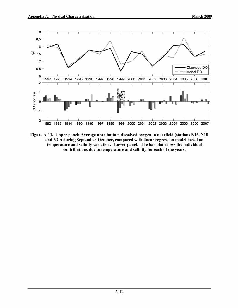
Appendix A: Physical Characterization March 2009
A-12
Figure A-11. Upper panel: Average near-bottom dissolved oxygen in nearfield (stations N16, N18
and N20) during September-October, compared with linear regression model based on temperature and salinity variation. Lower panel: The bar plot shows the individual
contributions due to temperature and salinity for each of the years.

Appendix B: Water Quality March 2009
B-1
B. WATER QUALITY This section presents a summary of 2007 water quality trends, and interannual comparisons of 2007 seasonal trends vs. 1992 to 2000 baseline and 2001 to 2006 post-diversion results. In 2007, trends in water quality parameters: nutrients, phytoplankton biomass [chlorophyll and particulate organic carbon (POC)], and dissolved oxygen were fairly consistent with those observed during previous years. A few noticeable differences were present, particularly in terms of the timing and magnitude of events. The most dominant feature of the year was the April Phaeocystis bloom. Over the course of the HOM program, a general sequence of water quality events has emerged from the data collected in Massachusetts and Cape Cod Bays. The trends are evident even though the timing and year-to-year manifestations of these events are variable. Typically a winter/spring phytoplankton bloom occurs as light becomes more available, temperatures increase, and nutrients are readily available. In recent years, the winter/spring diatom bloom has been typically followed by a bloom of Phaeocystis pouchetii in April. Late in the spring, the water column transitions from well-mixed to stratified conditions. This cuts off the nutrient supply to surface waters and terminates the spring bloom. The summer is generally a period of strong stratification, depleted surface water nutrients, and a relatively stable mixed-assemblage phytoplankton community. In the fall, as temperatures cool, stratification deteriorates and nutrients are again supplied to surface waters. This transition frequently contributes to the development of a fall phytoplankton bloom. Dissolved oxygen concentrations are lowest in the bottom waters prior to the fall overturn of the water column – usually in October. By late fall or early winter, the water column becomes well mixed and resets to winter conditions. This sequence is evident every year. The major features and differences from the baseline in 2007 are discussed below.
In early February nutrient concentrations were normal to slightly elevated relative to previous years for nitrate (NO3), but relatively low for silicate (SiO4). Satellite imagery (MODIS) suggests that winter productivity may have been relatively high in December and January, but that does not account for the disparity in NO3 (high) and SiO4 (low) concentrations. Although meteorological and physical oceanographic conditions were relatively normal in 2007, the lower river flows during the relatively dry, warm winter may have resulted in lower SiO4 concentrations. In February to early March the winter/spring diatom bloom was evident in Cape Cod Bay and at lower levels in coastal, Boston Harbor and nearfield areas resulting in reduced nutrient levels and elevated chlorophyll. Phaeocystis was first observed in the nearfield in March at low abundances in a mixed community along with diatoms. By early April the Phaeocystis bloom was at peak levels throughout the system. Diatoms were virtually nonexistent during the Phaeocystis bloom. By May, Phaeocystis was no longer present in the nearfield. As in 2005 and 2006, a bloom of the toxic dinoflagellates species Alexandrium fundyense was occurring in the Gulf of Maine in May 2007. Unlike the previous two years when northeasterly storms brought these blooms into the bays, however, meteorological conditions were such (SW winds predominant, limited NE winds) that the bloom primarily stayed offshore and Alexandrium abundances were comparable to 1992-2004 levels (≤10 cells/L). Late summer and fall conditions were generally typical. Physical factors dominated the water column with well-established stratification. Surface nutrients were depleted, and bottom DO concentrations steadily declined. Summer and fall diatom blooms were observed at Boston Harbor and coastal stations, and to a lesser degree in the nearfield in late September and October. Diatom abundances and resulting chlorophyll and particulate organic carbon (POC) concentrations were relatively low in comparison to previous fall blooms. Strong mixing/storms in late October and November returned the water column to winter, well-mixed conditions.

Appendix B: Water Quality March 2009
B-2
B.1 2007 Water Quality The nutrient data for 2007 generally followed the typical progression of seasonal events in Massachusetts and Cape Cod Bays. Maximum nutrient concentrations were observed in early February when the water column was well mixed and biological uptake of nutrients was limited (Figures B-1 to B-3). During the two February surveys, survey mean DIN concentrations (Figure B-1) were 11-13 µM in the nearfield and northern boundary, slightly lower at the offshore stations (10-11 µM), 7-10 µM at coastal and Boston Harbor stations, and lowest in Cape Cod Bay (<5 µM). Nitrate and silicate showed similar geographical trends with northern boundary, offshore and nearfield values being highest, Cape Cod Bay being lowest, and other areas in the middle (Figures B-2a and B-3a). Phosphate concentrations were less spatially variable, with most areas having similar concentrations, although Boston Harbor and Cape Cod Bay were somewhat lower (Figure B-3b). The lower nutrient concentrations seen in Cape Cod Bay were related to localized bloom of centric diatoms that also resulted in high chlorophyll and POC concentrations (Figure B-4; Appendix D). Ammonium in the nearfield was 1.5 µM in early February and the range at all other areas was <0.5 µM with a gradient of decreasing concentrations away from the shoreline.
Based on nutrient and plankton data from the March nearfield survey (WN073) and satellite imagery it appears that a minor spring diatom bloom may have occurred in Massachusetts Bay prior to the March 21st survey. The nutrient data from the March nearfield survey shows a moderate decline in all nutrients in the nearfield, including NH4 and SiO4 (Figures B-2 to B-3), and the plankton data shows a mixed diatom/Phaeocystis dominated community was present by late March. The satellite imagery shows moderate chlorophyll concentrations throughout the bays (especially close to shore and in Cape Cod Bay) on March 21 (Figure B-5). There was also a telltale drawdown and subsequent increase in SiO4 concentrations in the nearfield from February to March to April that is representative of diatom-to-Phaeocystis community change. Silicate is a required nutrient for diatoms but not utilized by Phaeocystis, so the SiO4 draw-down from February to March suggests that at least some portion of the bloom seen in the satellite imagery was related to diatoms, but the increase in concentrations from March to April seen in the nearfield data is indicative of Phaeocystis dominating the phytoplankton community assemblage, with silicate increasing due to remineralization. Although the early March diatom bloom likely drew down nutrients, there were sufficient nutrient levels remaining in the bay to support the large Phaeocystis bloom that appears to have been developing by mid March and peaking by mid April during the first leg of WF074 (Figure B-5). There was substantial decrease in nutrient concentrations by mid April. DIN levels had decreased by about 5 µM in Boston Harbor and Cape Cod Bay and from 8-11 µM in the other areas of Massachusetts Bay. The highest survey mean nutrient concentrations were observed furthest from the coast and the largest decreases in concentrations were also found in the nearfield, offshore and northern boundary areas (Figures B-1 to B-3). The dramatic decrease in nutrients was related to the Phaeocystis bloom occurring throughout the region. The relative changes in NO3 and PO4 concentrations during this survey (greatest decreases further offshore) correlate directly with the phytoplankton counts observed for the same period. Phaeocystis counts showed a large scale bloom present throughout the bays, but with highest abundances (6-9 million cells L-1) in the nearfield, northern boundary, and offshore areas. Wind/current data from the GoMOOS buoy A south of Cape Ann indicate that the Gulf of Maine waters were flowing into Massachusetts Bay during this time period and elevated surface fluorescence suggest that these waters were likely transporting Phaeocystis along with them (Figure B-6). The elevated Phaeocystis counts at nearfield, offshore, and northern boundary stations in April 2007 versus lower nearshore abundances also suggests that this may have represented the southern/western edge of an offshore bloom. Annual maxima in chlorophyll and POC concentrations were measured during this April bloom in the nearfield,

Appendix B: Water Quality March 2009
B-3
offshore, and northern boundary areas (Figure B-4). High POC concentrations were also observed in the Boston Harbor, but chlorophyll was not elevated proportionately. It is unclear whether the POC levels in the harbor were due to moderate to high (0.4 to 4.5 million cells L-1) abundance of Phaeocystis that had lower chlorophyll concentrations or if other terrestrial/near shore sources of organic carbon contributed to the high April POC levels. By May, the Phaeocystis bloom had ended and the organism was absent from the nearfield phytoplankton samples. Unlike the two previous years when red tide blooms of Alexandrium fundyense were well underway along the coastal waters of Maine, New Hampshire and into Massachusetts Bay, counts of Alexandrium in the nearfield were all ≤10 cells L-1, comparable to the low levels seen from 1992-2004. This is not to say there was not an Alexandrium bloom in 2007, just that it was not in the bays, but rather occurred well offshore in the Gulf of Maine and on Georges Bank (D. McGillicuddy, pers. com.). Winds and currents were not conducive to moving Gulf of Maine waters into the bays in May and June, but rather kept these waters well offshore. Survey mean nutrient concentrations in the nearfield reached or were close to annual minima during the May survey (Figures B-1 to B-3) and chlorophyll and POC concentrations had decreased sharply from the April peaks (Figure B-4). Nutrient, chlorophyll, and POC concentrations remained low in the nearfield and at other offshore stations (offshore, boundary, and Cape Cod Bay) over the summer. At Boston Harbor and coastal stations, nutrient levels were comparable to the other areas, but POC concentrations remained high from April to August (Figure B-4).
From August through October (and into November in the nearfield), survey mean nutrient concentrations increased. Surface nutrients remained low through the August farfield survey and September nearfield surveys, while survey mean nutrient concentrations continued to increase due to an increase in nutrient levels below the pycnocline. There was a slight increase in nearfield chlorophyll and POC concentrations in late September and October that was coincident with a minor fall diatom bloom, but overall phytoplankton biomass levels were relatively low in the offshore waters of the bays from June through November. Survey mean NH4 concentrations were quite variable in the nearfield over the course of the 2007 surveys: elevated in February, with other peaks in concentrations of >1 µM in the summer, early September, and November. This variability is likely due to a combination of biological and physical processes in the nearfield as well as sampling or missing peak concentrations in the effluent plume during each survey. Bottom water dissolved oxygen (DO) concentrations were elevated during the two February surveys and remained high or increased by about 1 mg L-1 to even higher levels in all regions by April when DO levels peaked coincident with the Phaeocystis bloom (Figure B-7). Following the crash of the Phaeocystis bloom after the April survey, bottom water DO concentrations and %-saturation declined steadily until June in the nearfield, harbor, coastal and Cape Cod Bay areas and into October in the offshore and boundary areas. The June mean bottom water DO concentrations establish setup conditions prior to the summer decline and can serve as a benchmark for interannual comparisons. In 2007, June DO concentrations were relatively low at the coastal and harbor stations as well as those in Cape Cod Bay (8.3-8.6 mg L-1) and higher levels were observed further offshore in Massachusetts Bay (9-10 mg L-1; Figure B-7a). A slight increase in production in the harbor and nearfield (see Figure C-1) along with a summer diatom bloom in coastal and harbor waters drove the increase in DO concentrations and %-saturation in these areas in August. By October, annual DO minima were observed across all areas of the bays and ranged from a low of 7.3 mg L-1 in the nearfield and offshore areas to 7.9 mg L-1 in Boston Harbor (Figure B-7a). Annual minima in DO %-saturation were also measured in October with the lowest levels of 76-78% for nearfield, offshore,

Appendix B: Water Quality March 2009
B-4
and northern boundary stations and the highest in the harbor ( 92%; Figure B-7b). Overall, bottom water DO levels were relatively high in 2007 and there were no issues or threshold exceedances.
B.2 Interannual Comparisons The water quality data for 2007 generally followed the typical progression of seasonal events in Massachusetts and Cape Cod Bays. The seasonal trends in nutrient concentrations are closely linked with both physical and biological factors. Physical mixing or stratification combined with biological utilization and remineralization act to increase or decrease the concentrations of nutrients over the course of each year. Nutrient concentrations are high in the winter when consumption is low and mixing is thorough; concentrations decrease in the surface waters during the winter/spring bloom due to consumption by phytoplankton, while the onset of stratification cuts off the supply of nutrients from deeper waters; as stratification strengthens nutrients are generally depleted in surface waters and increase at depth in the summer; nutrients then return to elevated levels in the surface waters following the fall bloom and mixing of the water column. Bottom water DO levels are typically at a maximum in the winter, decrease over the course of the summer during seasonal stratification, and reach annual minimum levels just prior to stratification breaking down in the fall – usually October. These cycles have been observed annually, with variation in magnitude and timing of events (e.g. Libby et al. 2006b).
B.2.a Nutrients Nearfield survey mean concentrations in 2007 generally followed baseline trends and are comparable in magnitude to the levels observed over the baseline period with some exceptions (Figures B-8 and B-9). In the previous section we mentioned that SiO4 levels in February were relatively low in comparison to the last couple of years and relative to NO3 concentrations (Figures B-2a and B-3a). Satellite imagery over the 06/07 winter suggested that there may have been elevated levels of productivity in the bays in December and January. This may have contributed to lower SiO4 levels, but would also have decreased levels of NO3. A more likely cause was that the relatively dry winter months, with reduced terrestrial runoff (see Figure A-2), may have led to lower levels of SiO4 loading to the system and the apparent difference between SiO4 and NO3 levels. However, when compared to baseline and other post-diversion data, the survey mean SiO4 concentrations in the nearfield are comparable to both the baseline and post-diversion means for the February surveys and it is the DIN and NO3 levels that are actually relatively high by comparison (Figures B-8 and B-9). The trends in 2007 nearfield nutrient concentrations, such as the spike in SiO4 concentrations associated with the April Phaeocystis bloom, were discussed in the previous section. In comparison to the baseline mean and range and post-diversion mean, the main differences in 2007 are the high DIN and NO3 in February and March, the high SiO4 in April, the low DIN and NO3 in April/May, and the relatively low NH4 concentrations versus all previous data in March to May and versus post-diversion data for most of the remainder of 2007 (early September and November excluded; Figures B-8 and B-9). It is unclear as to why the NO3 levels were so high in February and March 2007, but slightly higher NO3 concentrations have been observed overall since September 2000. The higher SiO4 and lower DIN and NO3 are related to the large Phaeocystis bloom as explained earlier. The relatively low NH4 concentrations, however, are more difficult to explain. As is typically the case, nearfield NH4 concentration trends tracked somewhat differently than the other nutrients. Due to its localized source at the outfall and the rapid and preferential consumption by phytoplankton, NH4 tends to vary on smaller temporal and spatial scales. Like NO3, NH4 was above the baseline range in early February. Ammonium concentrations dropped more quickly than the other nutrients declining to the baseline mean by late February, near the baseline minima in March and April, and below the baseline range by May (Figure B-9b). This is in contrast to the

Appendix B: Water Quality March 2009
B-5
post-diversion mean NH4 concentration trend of remaining 2±0.5 µM over most of the year. It is likely that the sampling intervals and spatial resolution with fixed stations are not able to clearly define the extent of the effluent plume on a survey-by-survey basis resulting in highly variable survey means. On average (over post-diversion period), there has been about a one micromolar increase in survey mean NH4 concentrations in the nearfield (Figure B-9b). The change in NH4 concentrations in the nearfield is consistent with model simulations which predicted that the transfer of effluent from Boston Harbor to Massachusetts Bay would greatly reduce nutrients in the harbor and increase them locally in the nearfield (Signell et al. 1996). This change was predicted to have little impact on concentrations in the rest of Massachusetts and Cape Cod Bays. The spatial patterns in NH4 concentrations in the harbor, nearfield and bays since the outfall diversion in September 2000 have consistently confirmed this. These spatial changes in NH4 are also manifested in annual mean concentrations for these areas. For example, the annual mean NH4 concentration in Boston Harbor dropped sharply from 2000 to 2001 (Figure B-10a). A sharp decrease was also seen at the coastal stations which are strongly influenced by water quality conditions in Boston Harbor. In contrast (and as expected), the increase in annual mean NH4 in the nearfield was not as dramatic as the harbor and coastal water decrease. Compared to 1999, the last full year before the bay outfall came online, annual mean NH4 levels in the nearfield almost doubled in 2001. However, since that time NH4 has shown a system-wide decrease and even in the nearfield concentrations are again comparable to the 1999 levels. This decline in NH4 over the past several years can be seen in all of the survey regions and current annual concentrations are comparable to 1992-1999 across the bays and are only slightly higher than in 2006, which was also very low. The overall shift in NH4 from pre- to post-diversion years can be seen in the contour plots showing the difference between the seasonal means from each period for the entire survey area (Figure B-11 top). The reduction in Boston Harbor and coastal water NH4 concentrations can be clearly seen across seasons, as well as the increase in NH4 at the bay outfall location. Most of these differences represent significant changes from baseline based on regression analyses (P<0.05). The trends in annual mean concentration for other inorganic nutrients are more variable. For example, NO3 (Figure B-11 bottom), has actually increased over much of the bays (except Boston Harbor) during the winter/spring and fall seasons. Year to year variability in NO3, SiO4, and PO4 appears to be related to the timing of sampling and occurrence of blooms than any clear trends in background levels.
B.2.b Phytoplankton Biomass Trends in chlorophyll and POC in 2007 were generally comparable to those observed during previous years, although there were some notable differences (Figures B-12 to B-14). Seasonal trends in phytoplankton biomass as measured by chlorophyll and POC are tied to physical conditions, nutrient availability, and ecosystem dynamics. The phytoplankton biomass seasonal signal in Massachusetts and Cape Cod Bays is dominated by winter/spring and fall blooms. Winter/spring phytoplankton blooms occur due to elevated growth related to increased light availability, nutrient replete conditions, and seasonal stratification of the physical environment that retains cells in the euphotic layer, prior to temperature-related increases in mortality due to grazing. Typically the timing of the fall bloom has been tied to decreased stratification and increased inputs of nutrients into the surface waters. In 2007 there was a typical, although weak, winter/spring diatom bloom (primarily in Cape Cod Bay, but also noted in the nearfield in March) followed by a large Phaeocystis bloom in April. Elevated abundances of diatoms were noted in the nearfield in August to October, but there was not a large fall bloom. Diatom abundances were higher in Boston Harbor and at coastal stations in August suggesting a nearshore bloom occurred.

Appendix B: Water Quality March 2009
B-6
In 2007 nearfield areal chlorophyll levels and POC concentrations were generally consistent with the baseline mean and seasonal patterns (Figure B-12). The winter/spring peak values in April for both chlorophyll and POC were higher than the baseline maxima and well above the post-discharge mean. There has been a slight shift in the winter/spring trends in these parameters that has been driven by both a tendency towards smaller winter diatom blooms and the consistent occurrence of March/April Phaeocystis blooms of moderate to high abundances since 2000. This change has also been observed at the offshore and northern boundary stations (Figure B-13). Rather than being dominated by February to March diatom blooms as during the baseline period, the trends in chlorophyll and POC are related to the April Phaeocystis blooms. The annual maximum chlorophyll and POC concentrations in these offshore Massachusetts Bay waters have consistently occurred during these April blooms since 2001. The 2007 and post-diversion mean areal chlorophyll and POC in the nearfield, offshore, and northern boundary closely tracked the baseline mean values over the rest of the year, though fall bloom levels tend to be lower than they had been during the baseline (Figures B-12 and B-13). In Boston Harbor, areal chlorophyll levels and POC concentrations were generally within the baseline range (Figure B-14). The main differences in 2007 were that areal chlorophyll was much higher than the baseline maximum in late February (a trend that has been observed in February since 2001) and that POC concentrations were below the baseline minimum in early February, but above the baseline mean from April to August. The annual pattern in areal chlorophyll concentrations was similar to that observed during the other post-diversion years, but the POC pattern was comparable to the pattern observed during baseline – low in winter, increasing to April and remaining high, before decreasing in the fall (Figure B-14). The chlorophyll data (along with production data presented in Appendix C) continue to suggest that the harbor may be changing from its previous pattern of chlorophyll and production levels peaking in summer to a more typical temperate coastal water trend dominated by the winter/spring bloom. The POC data in 2007, however, suggest that while this general trend may be emerging, that there is still wide year to year variability. Contour plots of pre- vs. post-diversion differences in phytoplankton biomass illustrate the decrease in both areal chlorophyll and POC concentrations at most of the Boston Harbor stations across each season (Figure B-15). The annual occurrence of moderate to major Phaeocystis blooms since 2000 and their impact on regional chlorophyll and POC levels is apparent in the overall increase in concentrations for both of these parameters during the post-diversion winter/spring. The plot for summer suggests an increase in POC levels in the nearfield post-diversion and this is confirmed by statistical analysis (see Table 4-1). The lack of fall blooms during the post-diversion period is evident in the lower chlorophyll and POC concentrations throughout most of Massachusetts and Cape Cod Bays (Figure B-15). Overall, the transfer of the outfall from Boston Harbor to the bay has likely contributed to the decreases observed in phytoplankton biomass as measured by chlorophyll and POC in the harbor. The changes (increases and decreases) in these parameters in the bays appear to be related to regional changes in dominant species and overall occurrence, or lack thereof, of blooms.
B.2.c Dissolved Oxygen Bottom water DO concentrations in 2007 followed trends that have been observed consistently since 1992. Bottom water DO levels are typically at a maximum in the winter, decrease over the course of the summer during seasonal stratification, and reach annual minimum levels just prior to stratification breaking down in the fall – usually October. Since the bay outfall came on line, there has been little change in the DO cycle in the nearfield and Stellwagen Basin and 2007 was no exception (Figure B-16). There is little difference between the baseline and post-diversion means and the only difference of note in 2007 were the slightly higher DO concentrations in April

Appendix B: Water Quality March 2009
B-7
associated with the bloom (Figure B-16). As discussed in Appendix A, bottom water DO levels in the bays are primarily driven by regional physical oceanographic processes and have been unaffected by the transfer to the bay outfall.
B.3 Water Quality Summary Water quality conditions in the bays in 2007 generally followed those observed previously, with some notable differences. Winter/spring phytoplankton abundance was once again dominated by Phaeocystis pouchetii, as it has been for the past seven years. Like 2005 and 2006, a minor diatom bloom preceded the emergence of Phaeocystis and contributed to the seasonal and yearly productivity. These two blooms were distinct, with diatoms peaking in mid March and declining by the time elevated Phaeocystis abundance was present in mid April. As observed during the previous blooms, the 2007 Phaeocystis bloom was a regional event with elevated abundances measured throughout the bays. Minor diatom blooms were observed in Boston Harbor and coastal stations and also the nearfield at lower abundances from August to October. Nutrient trends generally followed typical seasonal progressions. Nutrients concentrations were at a maximum in February, were depleted by phytoplankton consumption in the spring, remained low throughout the summer, began to increase as summer progressed into fall (increasing primarily in the bottom waters), and rebounded as cooler temperatures and fall storms returned the water column to well-mixed conditions in the fall. Dissolved oxygen levels were relatively high over most of the year and comparable to both baseline and post-diversion means. There were no DO or chlorophyll exceedances in 2007. As seen during the other post-transfer years, the primary change in comparison to the baseline is that NH4 has dramatically decreased in Boston Harbor and nearby coastal waters while increasing in the nearfield. Although the effluent plume is frequently observed in the nearfield, detectable levels appear to be confined to an area within 20 km of the outfall. Annual mean NH4 levels continued to be relatively low across the bays in 2007 and comparable to pre-1999 baseline values. In Boston Harbor, the decrease in NH4 has been concomitant with decreases in chlorophyll, POC, and production although an apparent change in the seasonal productivity from eutrophic to a more normal temperate coastal pattern first noted in 2003 has not continued to be observed. The higher nearfield NH4 concentrations have not translated into an obvious increase in biomass, whether measured as chlorophyll or POC.

Appendix B: Water Quality March 2009
B-8
0
3
6
9
12
15
Jan Feb Mar Apr May Jun Jul Aug Sep Oct Nov Dec
DIN
( μM
)
Boston Harbor Coastal Nearfield Offshore N. Boundary Cape Cod
Figure B-1. Time-series of survey mean DIN concentration in Massachusetts and Cape Cod Bays. Mean of concentrations over depths and stations within each region in 2007.

Appendix B: Water Quality March 2009
B-9
a) Nitrate
0
3
6
9
12
15
Jan Feb Mar Apr May Jun Jul Aug Sep Oct Nov Dec
NO
3 (μM
)
Boston Harbor Coastal Nearfield Offshore N. Boundary Cape Cod
b) Ammonium
0
1
2
3
4
5
Jan Feb Mar Apr May Jun Jul Aug Sep Oct Nov Dec
NH
4 (μM
)
Boston Harbor Coastal Nearfield Offshore N. Boundary Cape Cod
Figure B-2. Time-series of survey mean (a) NO3 and (b) NH4 concentration in Massachusetts and Cape Cod Bays. Mean of concentrations over depths and stations within each region in
2007.

Appendix B: Water Quality March 2009
B-10
a) Silicate
0
3
6
9
12
15
Jan Feb Mar Apr May Jun Jul Aug Sep Oct Nov Dec
SiO
4 (μM
)
Boston Harbor Coastal Nearfield Offshore N. Boundary Cape Cod
b) Phosphate
0.0
0.3
0.6
0.9
1.2
1.5
Jan Feb Mar Apr May Jun Jul Aug Sep Oct Nov Dec
PO4 (μM
)
Boston Harbor Coastal Nearfield Offshore N. Boundary Cape Cod
Figure B-3. Time-series of survey mean (a) SiO4 and (b) PO4 concentration in Massachusetts and Cape Cod Bays. Mean of concentrations over depths and stations within each region in
2007.
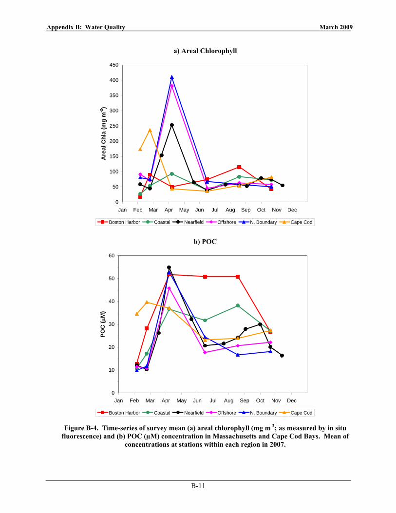
Appendix B: Water Quality March 2009
B-11
a) Areal Chlorophyll
0
50
100
150
200
250
300
350
400
450
Jan Feb Mar Apr May Jun Jul Aug Sep Oct Nov Dec
Are
al C
hla
(mg
m-2
)
Boston Harbor Coastal Nearfield Offshore N. Boundary Cape Cod
b) POC
0
10
20
30
40
50
60
Jan Feb Mar Apr May Jun Jul Aug Sep Oct Nov Dec
POC
( μM
)
Boston Harbor Coastal Nearfield Offshore N. Boundary Cape Cod
Figure B-4. Time-series of survey mean (a) areal chlorophyll (mg m-2; as measured by in situ fluorescence) and (b) POC (µM) concentration in Massachusetts and Cape Cod Bays. Mean of
concentrations at stations within each region in 2007.

Appendix B: Water Quality March 2009
B-12
March 21 (WN073) March 29 April 6
April 11 (WF074) April 20 (WF074) May 2
Figure B-5. MODIS chlorophyll images from March to May 2007.

Appendix B: Water Quality March 2009
B-13
(a) Chlorophyll Fluorescence
(b) Low-pass filtered Wind Stress and Ocean Currents
Figure B-6. GoMOOS buoy A data on (a) chlorophyll fluorescence in March through August 2007 and (b) wind stress and ocean currents for March and April 2007. GoMOOS buoy A01
plots generated online.

Appendix B: Water Quality March 2009
B-14
(a) DO Concentration
6
7
8
9
10
11
12
Jan Feb Mar Apr May Jun Jul Aug Sep Oct Nov Dec
Dis
solv
ed O
xyge
n (m
g/L)
Boston Harbor Coastal Nearfield Offshore N. Boundary Cape Cod
(b) DO Percent Saturation
60
70
80
90
100
110
120
Jan Feb Mar Apr May Jun Jul Aug Sep Oct Nov Dec
Dis
solv
ed O
xyge
n (%
Sat
urat
ion)
Boston Harbor Coastal Nearfield Offshore N. Boundary Cape Cod
Figure B-7. Time-series of average bottom dissolved oxygen (a) concentration and (b) percent saturation in Massachusetts and Cape Cod Bays. Mean of values from all stations within each
region in 2007.

Appendix B: Water Quality March 2009
B-15
(a) DIN
0
2
4
6
8
10
12
14
Jan Feb Mar Apr May Jun Jul Aug Sep Oct Nov Dec
DIN
( μM
)Baseline RangeBaseline Mean2007Post Mean
(b) Silicate
0
2
4
6
8
10
12
14
Jan Feb Mar Apr May Jun Jul Aug Sep Oct Nov Dec
SiO
4 (μM
)
Baseline RangeBaseline Mean2007Post Mean
Figure B-8. Time-series of survey mean (a) DIN and (b) SiO4 concentration in the nearfield in
2007 compared against the baseline range and mean (1992 to September 6, 2000) and post-diversion mean (September 7, 2000 to end of 2007). Data collected from all depths and all
nearfield stations. Note the nearfield baseline mean and range are shown for 17 surveys vs. 12 for 2007 and post-diversion.

Appendix B: Water Quality March 2009
B-16
(a) Nitrate
0
2
4
6
8
10
12
14
Jan Feb Mar Apr May Jun Jul Aug Sep Oct Nov Dec
NO
3 (μM
)Baseline RangeBaseline Mean2007Post Mean
(b) Ammonium
0
1
2
3
4
Jan Feb Mar Apr May Jun Jul Aug Sep Oct Nov Dec
NH
4 (μM
)
Baseline RangeBaseline Mean2007Post Mean
Figure B-9. Time-series of survey mean (a) NO3 and (b) NH4 concentration in the nearfield in 2007 compared against the baseline range and mean and post-diversion mean. Data collected
from all depths and all nearfield stations. Note the nearfield baseline mean and range are shown for 17 surveys vs. 12 for 2007 and post-diversion.

Appendix B: Water Quality March 2009
B-17
(a) Ammonium
0
2
4
6
8
10
1992
1993
1994
1995
1996
1997
1998
1999
2000
2001
2002
2003
2004
2005
2006
2007
NH
4 (μM
)
Boston Harbor Coastal Nearfield Offshore N. Boundary Cape Cod
(b) Nitrate
0
2
4
6
8
10
1992
1993
1994
1995
1996
1997
1998
1999
2000
2001
2002
2003
2004
2005
2006
2007
NO
3 (μM
)
Boston Harbor Coastal Nearfield Offshore N. Boundary Cape Cod
Figure B-10. Annual mean (a) NH4 and (b) NO3 concentration in Massachusetts and Cape Cod Bays. Mean of concentrations over depths, stations and surveys within each region. Dotted
line denotes offshore outfall online after 2000.

Appendix B: Water Quality March 2009
B-18
Winter/Spring Summer Fall
-71 -70.9 -70.8 -70.7 -70.6 -70.5 -70.4 -70.3 -70.2
41.9
42
42.1
42.2
42.3
42.4
42.5
42.6
-71 -70.9 -70.8 -70.7 -70.6 -70.5 -70.4 -70.3 -70.2
41.9
42
42.1
42.2
42.3
42.4
42.5
42.6
-71 -70.9 -70.8 -70.7 -70.6 -70.5 -70.4 -70.3 -70.2
41.9
42
42.1
42.2
42.3
42.4
42.5
42.6
-71 -70.9 -70.8 -70.7 -70.6 -70.5 -70.4 -70.3 -70.2
41.9
42
42.1
42.2
42.3
42.4
42.5
42.6
-71 -70.9 -70.8 -70.7 -70.6 -70.5 -70.4 -70.3 -70.2
41.9
42
42.1
42.2
42.3
42.4
42.5
42.6
-71 -70.9 -70.8 -70.7 -70.6 -70.5 -70.4 -70.3 -70.2
41.9
42
42.1
42.2
42.3
42.4
42.5
42.6
-5 -3 -1 1 3 Figure B-11. Change in seasonal NH4 (top row) and NO3 (bottom row) concentrations (µM) from baseline to post-diversion. Based on the difference of means calculated over all depths
from each station, survey, season, and period. Includes additional data collected at nine stations in Boston Harbor as part of MWRA’s Boston Harbor Water Quality Monitoring
(BHWQM) Program.

Appendix B: Water Quality March 2009
B-19
(a) Areal Chlorophyll
0
100
200
300
400
500
Jan Feb Mar Apr May Jun Jul Aug Sep Oct Nov Dec
Chl
orop
hyll
(mg
m-2
)Baseline RangeBaseline Mean2007Post Mean
(b) POC
0
10
20
30
40
50
60
70
Jan Feb Mar Apr May Jun Jul Aug Sep Oct Nov Dec
POC
( μM
)
Baseline RangeBaseline Mean2007Post Mean
Figure B-12. Time-series of survey mean (a) areal chlorophyll and (b) POC concentration in
the nearfield in 2007 compared against the baseline range and mean and post-diversion mean. Data collected from all depths and all nearfield stations. Note the nearfield baseline mean and
range are shown for 17 surveys vs. 12 for 2007 and post means.

Appendix B: Water Quality March 2009
B-20
(a) Areal Chlorophyll
0
100
200
300
400
500
Jan Feb Mar Apr May Jun Jul Aug Sep Oct Nov Dec
Chl
orop
hyll
(mg
m-2
)
Baseline RangeBaseline Mean2007Post Mean
0
100
200
300
400
500
Jan Feb Mar Apr May Jun Jul Aug Sep Oct Nov Dec
Chl
orop
hyll
(mg
m-2
)
Baseline RangeBaseline Mean2007Post Mean
(b) POC
0
10
20
30
40
50
60
70
Jan Feb Mar Apr May Jun Jul Aug Sep Oct Nov Dec
POC
( μM
)
Baseline RangeBaseline Mean2007Post Mean
0
10
20
30
40
50
60
70
Jan Feb Mar Apr May Jun Jul Aug Sep Oct Nov Dec
POC
( μM
)
Baseline RangeBaseline Mean2007Post Mean
Figure B-13. Time-series of survey mean (a) areal chlorophyll and (b) POC concentrations at
the offshore (left column) and north boundary (right column) regions in 2007 compared against the baseline range and mean and post-diversion mean. Data collected from all depths
and all stations.

Appendix B: Water Quality March 2009
B-21
(a) Areal Chlorophyll
0
100
200
300
400
500
Jan Feb Mar Apr May Jun Jul Aug Sep Oct Nov Dec
Chl
orop
hyll
(mg
m-2
)Baseline RangeBaseline Mean2007Post Mean
(b) POC
0
10
20
30
40
50
60
70
Jan Feb Mar Apr May Jun Jul Aug Sep Oct Nov Dec
POC
( μM
)
Baseline RangeBaseline Mean2007Post Mean
Figure B-14. Time-series of survey mean (a) areal chlorophyll and (b) POC concentration in the Boston Harbor in 2007 compared against the baseline range and mean and post-diversion
mean. Data collected from all depths at BWQM stations F23, F30, and F31.

Appendix B: Water Quality March 2009
B-22
Winter/Spring Summer Fall
-71 -70.9 -70.8 -70.7 -70.6 -70.5 -70.4 -70.3 -70.2
41.9
42
42.1
42.2
42.3
42.4
42.5
42.6
-71 -70.9 -70.8 -70.7 -70.6 -70.5 -70.4 -70.3 -70.2
41.9
42
42.1
42.2
42.3
42.4
42.5
42.6
-71 -70.9 -70.8 -70.7 -70.6 -70.5 -70.4 -70.3 -70.2
41.9
42
42.1
42.2
42.3
42.4
42.5
42.6
-50 -30 -10 10 30 50
-71 -70.9 -70.8 -70.7 -70.6 -70.5 -70.4 -70.3 -70.2
41.9
42
42.1
42.2
42.3
42.4
42.5
42.6
-71 -70.9 -70.8 -70.7 -70.6 -70.5 -70.4 -70.3 -70.2
41.9
42
42.1
42.2
42.3
42.4
42.5
42.6
-71 -70.9 -70.8 -70.7 -70.6 -70.5 -70.4 -70.3 -70.2
41.9
42
42.1
42.2
42.3
42.4
42.5
42.6
-5 -3 -1 1 3 Figure B-15. Change in seasonal areal chlorophyll (mg m-2; top row) and POC (µM; bottom
row) concentrations from baseline to post-diversion. Based on the difference of means calculated over all depths from each station, survey, season, and period. Includes additional
data collected at nine stations in Boston Harbor as part of MWRA’s BHWQM Program. Note that these additional BHWQM data show a much larger decline in POC levels than those
presented in Figure B-14.

Appendix B: Water Quality March 2009
B-23
(a) Nearfield
5
6
7
8
9
10
11
12
13
Jan Feb Mar Apr May Jun Jul Aug Sep Oct Nov Dec
DO
(mgL
-1)
Baseline RangeBaseline Mean2007Post Mean
(b) Stellwagen Basin
5
6
7
8
9
10
11
12
13
Jan Feb Mar Apr May Jun Jul Aug Sep Oct Nov Dec
DO
(mg
L-1)
Baseline RangeBaseline Mean2007Post Mean
Figure B-16. Time-series of survey mean bottom water DO concentrations in the (a) nearfield
and (b) Stellwagen Basin (stations F12, F17, F19 and F22) in 2007 compared against the baseline range and mean and post-diversion mean. Note the nearfield baseline mean and range
are shown for 17 surveys vs. 12 for 2007 and post means.

Appendix B: Water Quality March 2009
B-24
This page intentionally left blank

Appendix C: Productivity March 2009
C-1
C. PRODUCTIVITY This section provides an overview of the trends and magnitude of productivity in Massachusetts Bay in 2007 with particular focus on the nearfield sites (station N04 and N18). The higher frequency sampling in the nearfield permits a more detailed examination of temporal trends and interannual differences in productivity in Massachusetts Bay.
C.1 2007 Productivity Overview
C.1.a Nearfield Description With the exception of the fall bloom period, potential and measured productivity were similar at the nearfield sites throughout the seasonal cycle in 2007 (Figure C-1). The magnitude of the springtime peaks at both stations was higher than the baseline average (but not the range) (Figure C-2a and C-2b). The spring bloom magnitude at N04 was less than at N18, which is similar to the pattern seen in 2002 and 2003 but a change in the pattern seen since 2004 (Figure C-3). The magnitude of the fall blooms at N18 and N04 were low in comparison to baseline and early post-diversion fall blooms and similar to levels observed since 2003 (Figure C-4).
The winter-spring blooms observed at nearfield stations in 1995-2006 generally reached values of 2,000 to 4,500 mg C m-2 d-1, with bimodal peaks often occurring in February - April. The bloom in 2007 reached maximum measured values at the nearfield sites of ~1,765 – 2,070 mg C m-2 d-1 with unimodal peaks observed in late April. Unlike many years, an early February peak was not observed. Although the timing differed, the magnitude of the nearfield winter-spring bloom peaks in 2007 were similar to values observed from 2003 -2006, a period characterized by relatively low magnitude winter spring blooms. The onset of stratification and depletion of nitrogen in the surface waters coincided with the cessation of the spring bloom as in prior years.
C.1.b. Boston Harbor Description At the harbor station (F23), areal productivity (potential and measured) increased over the spring period, declined slightly in April, reached an annual peak in August and declined in the fall (Figure C-1). The pattern is similar to that observed since the outfall diversion. Prior to the diversion, productivity generally increased from spring to mid-summer then declined in the fall. With the exception of the early springtime period, production values were low relative to the long term mean throughout the annual cycle (Figure C-2c). Prior to the outfall diversion, peak productivity most frequently occurred in the early summer while during the post outfall period peak production consistently occurred either in the spring or the fall, until 2006. With only one year since 2000 showing a major spring bloom it does not seem likely that the harbor station is rapidly shifting to the nearfield pattern, but the overall decline in productivity seen at the station does indicate a shift to a less-enriched environment (Figure C-5).
C.2 Interannual Comparisons
C.2.a Areal Productivity To assess the potential effects of the September 2000 relocation of effluent discharge from Boston Harbor to Massachusetts Bay on areal productivity, we compared production measurements at the nearfield and the Boston Harbor stations in 2007 to the baseline productivity data collected from February 1995 to August 2000 (Figure C-2). At nearfield stations and in the harbor, areal production for 2007 was less than the baseline average for almost all data points. The exceptions were in late-April during the Phaeocystis bloom and during the fall bloom peak at the nearfield sites,

Appendix C: Productivity March 2009
C-2
both of which were just above the baseline mean. All other data points for the year were lower than the baseline average at these two stations.
At the Boston Harbor station, productivity in 2007 fell well below the baseline mean during the summer and fall but was slightly higher than the baseline mean in the early spring (February – March).
C.2.b Regional Changes in Bloom Magnitude Examining the magnitude of seasonal blooms at the nearfield (average for stations N04 and N18) and farfield (station F23) sites indicates that the greatest effect of the outfall relocation is apparent in seasonal productivity levels in the harbor (Figure C-6). For this seasonal bloom analysis, the peak productivity from each season (February-April, May-August, and September-December) and year were averaged for both the pre- and post-diversion periods. The magnitude of the spring bloom in the harbor decreased from a mean of 2,118 mg C m-2 d-1 pre-relocation to 1,263 mg C m-2 d-1 post-relocation (Figure C-6a). During the same period, the nearfield values for the spring maximum decreased slightly from 2,547 mg C m-2 d-1 to 2,287 mg C m-2 d-1, respectively. During the summer, the harbor showed a similar pattern with a post-diversion mean of 1,141 mg C m-2 d-1 compared to a pre-diversion mean of 2,617 mg C m-2 d-1 (Figure C-6b). The peak nearfield values are somewhat lower post-diversion (1,292 mg C m-2 d-1) compared with pre-diversion (1,677 mg C m-2 d-1) during the summer. During the fall, the values for the harbor followed the same pattern as the other seasons with high values pre-diversion (3,206 mg C m-2 d-1) and low values post-diversion (1,808 mg C m-2 d-1) (Figure C-6c). Again, a slight decrease was seen in fall productivity in the nearfield (2,660 mg C m-2 d-1 pre and 2,327 mg C m-2 d-1 post).
Prior to the outfall relocation in 2000, the typical harbor pattern had low winter/spring production and high production in the summer which was maintained into the fall. After 2000, winter production (February) increased slightly in the harbor (Figure C-5) although productivity throughout the entire spring bloom period (February – April) declined (due to a sharp decline in April production). Summer and fall production in the harbor also decreased. Fall production did not decrease as much as the summer, however, corresponding to the appearance of a fall “bloom” in the harbor. In the nearfield, mean production values decreased slightly for spring, summer, and fall. As seen in Table C-1, the change in the magnitude of the summer bloom at station F23 is significant while the other seasonal changes discussed above are not.
Table C-1. Comparison of peak spring, summer, and fall productivity (mg C m-2 d-1) and annual productivity (g C m-2 y-1) during the pre- and post-diversion periods at the harbor station (F23) and the nearfield stations (N16/18, N04). Results presented are change in productivity from pre- to post-
diversion and P values for ANOVAs based on non-transformed data (n = 13; tests for non-normality were not significant). Significant results at P≤0.05 denoted with an asterisk.
Station F23 Station N16/N18 Station N04 Variable Change P Change P Change P
Spring Peak -855 0.34 -649 0.41 +129 0.83 Summer Peak -1,476 0.05* -687 0.23 -52 0.91 Fall Peak -1,398 0.17 -648 0.45 -8 0.99 Annual Prod -279 0.03* -110 0.17 +11 0.64

Appendix C: Productivity March 2009
C-3
C.2.c Annual Productivity Potential annual productivity (g C m-2 y-1) is calculated by trapezoidal integration of potential daily productivity (mg C m-2 d-1) over the year. For the period prior to the February survey and after the last survey of the year, we assume that the initial and final measured values over the annual cycle are acceptable estimates for these periods not measured. Figure C-7 compares potential annual productivity during pre and post outfall years (data from 2000 are not included in the analysis since the outfall became operational that year). Annual productivity values decreased at station N18 by 110 g C m-2 y-1 and in Boston Harbor by 279 g C m-2 y-1 and increased slightly at station N04 by 11 g C m-2 y-1, The most notable changes since the outfall relocation are the large decreases in annual productivity within the harbor, the decline in mean annual productivity at all stations since 2002, and the similarity in mean annual productivity among at all three sites during the post-outfall period. As seen in Table C-1 the decrease in annual productivity at the Boston Harbor station is significant (P = 0.03) while decreases at the nearfield sites are not significant. Figure C-8 and Table C-2 indicate that annual productivity has declined at both nearfield sites and the harbor station in recent years (2003-2007). Annual productivity has been near (harbor) or below (nearfield) 300 g C m-2 y-1 since 2003. The timing of this apparent decrease three years after the diversion suggests that a change may be occurring system-wide resulting in lower primary productivity that is unrelated to the outfall relocation. Since 2003 annual productivity is similar and lower at all 3 sites relative to earlier years. Although annual productivity at the nearfield sites is not significantly different pre- and post-diversion (Table C-1), the results are significant when comparing the period from 1995-2002 versus 2003-2007 (Table C-3). In addition, there is a significant decrease in the fall productivity peak that was not apparent when comparing pre- and post-diversion periods (Table C-3). This makes it difficult to rule out a small local difference in productivity in the nearfield (compared to the rest of the region, where productivity is not measured) since diversion. But the data do show that the outfall has not caused detrimental or even anomalous increases in production.
Table C-2. Potential annual productivity (g C m-2 y-1) at stations F23, N16/N18, and N04 from 1995-2007.
Stations Year F23 N16/N18 N04 1995 786 426 3061996 818 529 3691997 731 558 4271998 224 213 1921999 659 503 3952000 494 664 5112001 404 551 5692002 587 607 5322003 326 291 2932004 333 201 2382005 234 198 2812006 313 247 2722007 356 252 258

Appendix C: Productivity March 2009
C-4
Table C-3. Comparison of peak spring, summer, and fall productivity (mg C m-2 d-1) and annual productivity (g C m-2 y-1) during the periods 1995-2002 and 2003-2007 at the harbor station (F23) and the nearfield stations (N16/18, N04). Results presented are differences in
productivity from 1995-2002 to 2003-2007 and P values for ANOVAs based on non-transformed variables (n = 13). Significant results at P≤0.05 denoted with an asterisk.
Station F23 Station N16/N18 Station N04 Variable Change P Change P Change P
Spring Peak -1,286 0.16 -1,328 0.08 -482 0.42 Summer Peak -995 0.09 -890 0.12 -550 0.21 Fall Peak -1,351 0.18 -2,111 0.003* -1,062 0.01* Annual Prod -276 0.01* -269 0.002* -144 0.03*
C.3 Productivity Summary In 2007, the patterns of productivity seen at both the nearfield and farfield (Boston Harbor) stations were somewhat different from the long-term patterns (1995 – 2002) but similar to the values seen in recent years (2003 -2006). The major differences with long term trends were the reduced annual productivity at all three sites and the lower magnitude of the spring and fall bloom peaks at the nearfield stations in recent years. These differences may however reflect the reduced temporal resolution of the sampling scheme relative to earlier years, and may not be related to actual changes within the system. At both nearfield stations, the timing of the spring bloom onset was later (April 21) than all previous years except 1995 (April 24). Productivity decreased by late May in the nearfield region signifying the termination of the spring bloom. In the harbor, a moderate spring bloom was observed in early March, lower in magnitude than the blooms observed in 2002 – 2006, with a fall seasonal productivity maximum in late August. Production at all three stations throughout much of the annual cycle was below the long-term mean. At the nearfield sites, production was below the long-term means on all occasions except the spring and fall peak bloom production. Interannual patterns show that production in Boston Harbor has significantly decreased post-relocation of the outfall. In the nearfield production has declined slightly since the outfall relocation but the change is not significant. Compared to previous years the reduced magnitude of the annual production and the reduced spring and fall bloom peak at both nearfield stations are the most significant events in 2007.

Appendix C: Productivity March 2009
C-5
F23
0
500
1000
1500
2000
J F M A M J J A S O N D
mg
C m
-2 d
-1
Measured Potential
N04
0
500
1000
1500
2000
J F M A M J J A S O N D
mg
C m
-2 d
-1
Measured Potential
N18
0
1000
2000
3000
J F M A M J J A S O N D2007
mg
C m
-2 d
-1
Measured Potential
Figure C-1. Measured and potential areal production (mgCm-2d-1) in 2007 at stations F23,
N18, and N04.

Appendix C: Productivity March 2009
C-6
F23
0
2000
4000
6000
8000
Jan Feb Mar Apr May Jun Jul Aug Sep Oct Nov Dec
mg
C m
-2 d
-1Baseline Range
Baseline Mean
2007
N18
0
1000
2000
3000
4000
5000
Jan Feb Mar Apr May Jun Jul Aug Sep Oct Nov Dec
mg
C m
-2 d
-1
Baseline Range
Baseline Mean
2007
N04
0
1000
2000
3000
4000
5000
Jan Feb Mar Apr May Jun Jul Aug Sep Oct Nov Dec
mg
C m
-2 d
-1
Baseline Range
Baseline Mean
2007
Figure C-2. Time-series of areal production (mgCm-2d-1) at stations F23, N18, and N04 for
2007 compared against baseline range and mean (1995 to September 2000). Note the nearfield station baseline mean and range are shown for 17 surveys vs. 12 in 2007.

Appendix C: Productivity March 2009
C-7
Spring Bloom PeakAreal Productivity
0
1000
2000
3000
4000
5000
6000
1994 1995 1996 1997 1998 1999 2000 2001 2002 2003 2004 2005 2006 2007
mg
C m
-2 d
-1F23 N16/N18 N04
Figure C-3. Spring bloom peak potential areal productivity (mgCm-2d-1) at stations F23,
N16/N18, and N04.
Fall Bloom Peak Areal Productivity
0
1000
2000
3000
4000
5000
6000
1994 1995 1996 1997 1998 1999 2000 2001 2002 2003 2004 2005 2006 2007
mg
C m
-2 d
-1
F23 N16/N18 N04
7,583
Figure C-4. Fall bloom peak potential areal productivity (mgCm-2d-1) at stations F23,
N16/N18, and N04.

Appendix C: Productivity March 2009
C-8
0
1000
2000
3000
4000
Jan Feb Mar Apr May Jun Jul Aug Sep Oct Nov Dec
Prod
uctiv
ity (m
g C
m-2
d-1
) Baseline
Post-transfer
Figure C-5. Time-series of pre- (1995 to September 2000) and post-diversion areal production
(mgCm-2d-1) at station F23. Error bars represent ± SE.

Appendix C: Productivity March 2009
C-9
Spring Bloom Peak Areal Productivity
0
1000
2000
3000
4000
5000
Harbor Nearfield
mg
C m
-2 d
-1PrePost
Summer Bloom Peak Areal Productivity
0
1000
2000
3000
4000
5000
Harbor Nearfield
mg
C m
-2 d
-1
PrePost
Fall Bloom Peak Areal Productivity
0
1000
2000
3000
4000
5000
Harbor Nearfield
mg
C m
-2 d
-1
PrePost
Figure C-6. Spring, summer, and fall bloom peak production (mgCm-2d-1) at nearfield (N04
and N16/N18) and Boston Harbor (F23) stations. Pre- vs. post-diversion – spring and summer 95-00 vs. 01-07 and fall 95-99 vs. 00-07.

Appendix C: Productivity March 2009
C-10
0
200
400
600
800
F23 N16/N18 N04
g C
m-2
y-1
Pre Post
Figure C-7. Potential annual production (gCm-2yr-1) for stations F23, N16/N18, and N04 pre- (1995-
1999) and post- (2001-2007) diversion.
0
100
200
300
400
500
600
700
800
900
1994 1995 1996 1997 1998 1999 2000 2001 2002 2003 2004 2005 2006 2007
Prod
uctiv
ity (g
C m
-2 y
-1)
F23 N16/N18 N04
Figure C-8. Potential annual production (gCm-2yr-1) for stations F23, N16/N18, and N04 from
1995 to 2007.

Appendix D: Plankton March 2009
D-1
D. PLANKTON In 2007, most trends in phytoplankton and zooplankton abundance, species composition and bloom cycles were generally consistent with those observed in previous years, although timing and magnitude of events were sometimes different. The main stories in 2007 relative to previous years were the continued decreased level of diatoms (especially summer and fall) and a large, regional Phaeocystis bloom (comparable to the large blooms in 2000 and 2004). The 2007 zooplankton community consisted of a typical assortment of species and abundance, and followed typical seasonal patterns that generally follow temperature, with low abundance levels in winter, rising through spring to maximum summer levels, and declining in the fall. There had been a sustained decline in total zooplankton from 2001 to 2006, due primarily to decreases in copepods and nauplii. This trend appears to have reversed itself in 2007 with higher abundances of total zooplankton and copepods, though copepod nauplii were still observed in abundances lower than the long term average.
D.1 Phytoplankton Summary
D.1.a Total Phytoplankton Total phytoplankton abundance in the nearfield in 2007 was dominated by the large Phaeocystis bloom in April (~8 x 10⁶ cells L-1) and showed a secondary peak in abundance of ~2 x 10⁶ cells L-1 in September/early October that was diatom- and microflagellate- dominated (Figure D-1). The bi-modal pattern in total phytoplankton abundance is more apparent in Figure D-2 with a large; Phaeocystis dominated spring (April) peak of 2.4 to 9.1 x 10⁶ cells L-1 and the secondary late summer/Autumn bloom peak of 2 to 3 x 10⁶ cells L-1. Total phytoplankton abundance varied by region, but there was no consistent pattern of regional differentiation in total phytoplankton abundance (Figure D-2). The range of total nearfield phytoplankton abundance observed during 2007 was similar to that observed in previous years with the exception of elevated phytoplankton abundance during the April Phaeocystis bloom (Figure D-3).
D.1.b Microflagellates Microflagellates were the numerically dominant component of Massachusetts Bay and Cape Cod Bay phytoplankton during 2007, consistent with previous observations. Microflagellates comprised an average of 59% numerically of the total phytoplankton during 2007. Past observations indicate that the microflagellate annual cycle generally tracks the water temperature annual cycle, featuring a winter minima and summer maxima. Consistent with this, during 2007 nearfield microflagellate abundance increased from ~0.4 x 10⁶ cell L-1 in February to 1.6 x 10⁶ cell L-1 in September with a slight decrease in June and July (Figure D-4). By late October and the last observations of the year in November microflagellate abundance had declined to 0.75 - 1.3 x 10⁶ cell L-1. Comparison of the 2007 nearfield microflagellate annual cycle to that of previous years revealed elevated winter (February and March) microflagellate abundance and a notable summer (June and July) dip in microflagellate abundance (Figures D-4 and D-5). While June and July microflagellate abundance observations were well within the range of baseline observations, the summer depression in microflagellate abundance to <1 x 10⁶ cell L-1, combined with the large April Phaeocystis bloom, was largely responsible for the bi-modal shape of the 2007 total phytoplankton annual abundance cycle (i.e., Figure D-2). By September, and especially during early October 2007, microflagellate abundance had rebounded, with the early October 2007 nearfield mean value (1.43 x 10⁶ cell L-1) slightly greater than the October maximum baseline range value (Figure D-5). Elevated nearfield microflagellate abundance was also recorded during November 2007. Note that elevated early winter (February and March) and elevated November microflagellate abundance appears to be a persistent and distinctive feature of the post-diversion period (Figure D-5).

Appendix D: Plankton March 2009
D-2
D.1.c Cryptomonads Unidentified cryptophytes were the second most numerically dominant component of the phytoplankton on average comprising ~15% of the phytoplankton cells observed in 2007. The contribution of cryptophytes to total phytoplankton in the nearfield region varied from 1% during the April 2007 Phaeocystis bloom to a maximum of 27.5% during July 2007 (Figure D-1). Other regions followed a similar pattern. The 2007 cryptophyte annual cycle had a general pattern of reduced abundance of ~100,000 cells L-1 from February through April, increasing to levels of 200,000 to 450,000 cells L-1 during May to October, followed by a return to low winter levels of about 100,000 cells L-1 in November (Figure D-6). Cryptophyte abundance during 2007 was generally elevated compared to baseline mean levels for the nearfield region and above the baseline range for February to March, May, and August (Figure D-7). February and March 2007 nearfield cryptophyte abundance levels were 80,000 to 100,000 cells L-1 compared to baseline mean levels of ≤50,000 cells L-1. May and October 2007 had the greatest increases in cryptomonad abundance relative to baseline levels. During these two months, cryptomonad abundance was elevated 2- to 3-fold relative to the respective baseline mean levels. May 2007 nearfield cryptomonad abundance of 317,000 cells L-1 was >3 times higher than the baseline mean May level of 91,000 cells L-1 and higher than the baseline maximum (Figure D-7). Summer levels from June to August continued to about double the baseline mean and in August they were higher than the baseline maximum. The October 2007 nearfield cryptomonad abundance was also double the baseline mean level, though still within the range. A pattern of long-term increased cryptomonad abundance in the nearfield may be emerging, based on the relative increase in 2007 cryptophyte abundance and elevated post transfer cryptophyte abundance relative to baseline levels.
D.1.d Diatoms Numerically, diatoms comprised a small portion of the phytoplankton observed in the nearfield in 2007 (Figure D-1). In contrast to the smaller microflagellates and the April-blooming Phaeocystis, diatoms comprised only 11% of the phytoplankton observed during 2007. Massachusetts Bay diatoms are predominantly centric diatoms, with only occasional blooms of pennate diatoms (notably Thalassionema and Pseudo-nitzschia spp.), so combined centric and pennate diatom abundance is presented here. Key diatom species or genera that dominated nearfield diatom abundance during 2007 include the emergence of Dactyliosolen fragilissimus as a summer bloom former, particularly in the nearfield and coastal regions. D. fragilissimus was responsible for the summer 2006 chlorophyll-concentration exceedance, and was also present at elevated levels during the summer of 2005. While summer blooms of D. fragilissimus present no known harmful impacts, the 2005-2007 summer increase in this species is a notable recent phenomenon, although elevated levels occurred in 1995 and 2002. Diatom abundance varied widely during 2007 with, for example a ~60-fold range in nearfield diatom abundance between the minimum level (6,400 cells L-1) during June (mostly Thalassiosira and Chaetoceros spp.) and the maximum nearfield abundance level (373,000 cells L-1) observed in early October (dominated by Guinardia delicatula, Skeletonema costatum, and Leptocylindrus danicus). The overall 2007 diatom annual cycle was bi-modal, with elevated winter-spring and late summer to autumn periods separated by a June nadir in diatom abundance (Figure D-8). There appeared to be a consistent regional pattern in diatom abundance, with increased diatom abundance in the Cape Cod, coastal, and harbor regions relative to the nearfield, north boundary and offshore regions (Figure D-8). For example, diatom abundance in late February was 2.1 to 2.9 x 10⁵ cell L-1 in the Cape Cod, coastal and harbor regions compared to levels of 2.1 to 6.3 x 10⁴ cell L-1 in the nearfield, north boundary and offshore regions. This winter-spring bloom observation may be partially explained by an earlier winter-spring bloom initiation in relatively shallow Cape Cod Bay, however, diatom

Appendix D: Plankton March 2009
D-3
abundance was consistently higher than that observed in the nearfield in the Cape Cod, coastal and harbor regions in all six of the 2007 farfield surveys (Figure D-8). Nearfield diatom abundance in 2007 was low relative to previous (1992-2006) observations (Figure D-9). February nearfield diatom abundance was below that of the baseline minimum, and all 2007 nearfield observations were below the baseline mean level (Figure D-9). Further, while March through June 2007 nearfield diatom abundance was near that of the post-diversion mean, 2007 nearfield diatom abundance was below that of the post-diversion mean level from July through November. Reduced diatom abundance appears to be part of a long-term post-2000 trend of declining nearfield diatom abundance (Libby et al. 2007). The reduced diatom abundance noted for the nearfield appears to be part of a region-wide long-term post-diversion trend of declining nearfield diatom abundance (Libby et al. 2007). While in-depth statistical analysis of the post-2000 regional diatom decline will be completed in future reports, we note that a preliminary regional comparison of pre- and post-diversion diatom abundance indicated that diatom abundance declined in all regions. Greatest declines of ~70% were noted in the offshore and Cape Cod Bay regions, a decline of about 50% was noted in the coastal region and a 30% decline in diatom abundance was observed in the nearfield and harbor regions."
D.1.e Dinoflagellates Dinoflagellates were a relatively minor component of the phytoplankton community during 2007, comprising an average of 4% of total phytoplankton numerically. Regionally averaged dinoflagellate abundance estimated from >20 μm screened water counts varied greater than 50-fold seasonally from less than 50 cells L-1 (observed at the coastal, harbor, boundary, offshore and nearfield regions during February) to about 2,500 cells L-1 (observed in the harbor in August). Dinoflagellate abundance was greatest during the summer months with a June peak in the nearfield and a broader, region-wide August through November peak (Figure D-10). Ceratium spp. (predominantly C. longipes, C. tripos, C. fusus) were a major component of >20 μm screened dinoflagellate abundance, with nearfield Ceratium spp. achieving an abundance peak of 1,049 cells L-1 during June, with abundances of 590 cells L-1 and 464 cells L-1 observed during July and October, respectively. While a summer peak in Ceratium abundance was observed in the nearfield, coastal and Cape Cod regions, Ceratium had an October peak (1,300 to 1,700 cells L-1) in its annual cycle in offshore and boundary regions. Other abundant dinoflagellates in the nearfield during 2007 included Scrippsiella trochoidea which achieved levels of 200 cells L-1 during September and 300 cells L-1 during October and Protoperidinium spp. which sustained levels of 300 to 550 cells L-1 during August and September in the nearfield. Alexandrium fundyense was observed in low abundance levels of <10 cells L-1 in the nearfield during the spring of 2007. Nearfield >20μm dinoflagellate abundance was reduced compared to baseline and post-diversion mean levels during 2007 (Figure D-11). Nearfield dinoflagellate abundance was below the post-diversion mean level in all months except July and September and abundance was below the baseline abundance level during all months sampled (February -November) during 2007. Nearfield >20 µm dinoflagellate abundance during winter (February and March) 2007 was most drastically reduced compared to baseline levels, with winter 2007 dinoflagellate abundance in the tens of cells L-1 compared to baseline mean levels of hundreds of cells L-1.
D.1.f Nuisance Species Three harmful or nuisance phytoplankton, Pseudo-nitzschia spp., Alexandrium fundyense and Phaeocystis pouchetii, were observed during 2007 MWRA monitoring. Pennate diatoms in the genus Pseudo-nitzschia were observed at low levels of up to ~200 cells L-1 during February and March 2007

Appendix D: Plankton March 2009
D-4
(Figure D-12). Such levels are far below those recorded in previous years (i.e., >150,000 cells L-1 observed during February of 1999) and are also far below any contingency plan threshold or level that would caused amnesiac shellfish poisoning. Similarly, while cells of the dinoflagellate Alexandrium fundyense, responsible for paralytic (saxitoxin) shellfish poisoning (PSP), were observed during 2007 in the MWRA monitoring regions of Massachusetts and Cape Cod Bays, the maximum observation was <10 cells L-1 (Figure D-13) far below caution levels, and far below the maximum level of 36,830 cells L-1 observed in the nearfield during the May 2005 Alexandrium red tide event. Low Alexandrium fundyense populations in Massachusetts Bay during 2007 is consistent with the observation that the coastal plume responsible for transporting Alexandrium cells into Massachusetts Bay in 2005 and 2006 was pushed offshore to the Georges Bank area during spring 2007 (Don Anderson pers. comm.). The most prominent nuisance phytoplankton event during 2007 was the April bloom of the colonial prymnesiophyte Phaeocystis pouchetii (Figure D-14). The 2007 levels of Phaeocystis (survey mean of 7.8 million cells L-1 in the nearfield in April) rivaled those of the 2004 bloom, which was the largest recorded during 1992-2007 monitoring (Figure D-14). The 2007 Phaeocystis bloom was observed in all regions of the bays, consistent with past observations (Libby et al. 2007). However, the 2007 Phaeocystis bloom was of moderate duration, with Phaeocystis cells observed only from late February to early April for a bloom duration of approximately 30 days. By comparison, Phaeocystis blooms of up to 100 days duration have been observed in some years (i.e., 2003 and 2005).
D.1.g Interannual Phytoplankton Trends Phytoplankton communities are mixtures of many species, with the abundance and composition of the community changing due to each species’ responses to changing environmental influences on the habitat (e.g. annual changes in irradiance, temperature, nutrient, grazer abundance). A “normal” seasonal succession in Massachusetts and Cape Cod Bay has been observed since 1992. In whole-water phytoplankton samples, microflagellates and cryptomonads are usual numerical-dominants throughout the year, and their abundance generally tracks water temperature, being most abundant in summer and least abundant in winter. In addition to microflagellates, the following taxa are also dominant in Massachusetts and Cape Cod Bays during the periods identified below:
Winter (primarily February) and Spring (March, April) – diatoms are usually abundant, including species of the genera Chaetoceros and Thalassiosira, Guinardia delicatula, and spring blooms of Phaeocystis pouchetii (mainly in April);
Summer (May, June, July, August) – microflagellates are at peak abundance, with cryptomonads and the diatoms Skeletonema costatum, Leptocylindrus danicus, Dactyliosolen fragilissimus, Guinardia delicatula, and various species of Chaetoceros;
Fall (September through December) – diatoms are usually abundant, including Asterionellopsis glacialis, Guinardia delicatula, Skeletonema costatum, Dactyliosolen fragilissimus, Leptocylindrus minimus, L. danicus, as well as cryptomonads, and assorted gymnodinoid dinoflagellates.
Superimposed over the background dominance of microflagellates, cryptomonads, and common diatoms, in some years, there are major blooms of a single species such as Asterionellopsis glacialis in fall of 1993 or Phaeocystis pouchetii in spring of 1992, 1994, 1997, and every year since 2000 (Figure D-14). The interannual variability associated with both magnitude and occurrence of various blooms as represented by total phytoplankton abundance is shown in Figure D-15. Although such blooms may be intermittent, they tend to occur regionally and are usually observed throughout

Appendix D: Plankton March 2009
D-5
Massachusetts and Cape Cod Bay and beyond. Why such species bloom in some years but not others remains unclear. In 2007, total nearfield phytoplankton abundance was generally within the baseline range and close to the baseline mean (Figure D-3), with the exception of the high April abundance during the Phaeocystis bloom.
D.2 Zooplankton Summary
D.2.a 2007 Zooplankton Summary Zooplankton assemblages in 2007 were dominated, as in all previous years, by copepod nauplii and copepods (Figures D-16 to D-18). Most of the copepods were Oithona similis copepodites and adults. Barnacle larvae comprised approximately half of the animals collected in Boston Harbor in late February 2007 (Figure D-16a). Total zooplankton abundance has consistently followed a seasonal cycle with low abundance during the colder months, rising through spring to maximal levels during the summer, and declining again in the fall. This was the case in 2007 (Figures D-16 to D-18). All areas had maximum abundance in June and October. Zooplankton in Cape Cod Bay was higher in early February than in other areas, and Cape Cod Bay was the only area where total abundances in February exceeded 20,000 animals m-3 (Figure D-18b). Means for total zooplankton abundance in the nearfield in 2007 were generally low (Figure D-19). The 2007 means were below the baseline mean for all periods except for early October. Nearfield means were also below the baseline range throughout February and March, and again in mid-July mainly due to low levels of copepodites and adult copepods (Figure D-20a), primarily Oithona similis (Figure D-21a). Nearfield means for 2007 abundances of copepod nauplii were within the baseline range, except for low values in mid-July (Figure D-20b). Similar means for Calanus finmarchicus copepodites and adults were within the baseline range, except for slightly higher values in August (Figure D-21b).
D.2.b Long-term Zooplankton Community Structure The variability in abundance and structure of the zooplankton community in 2007 in Massachusetts and Cape Cod Bays appears similar to patterns recorded since the beginning of sampling in 1992. The main difference has been the lower overall abundance of zooplankton since 2001 (Figure D-22). In order to explore this apparent change more closely, time series analysis (Broekhuizen and McKenzie 1995) was applied to the dominant zooplankton groups in the nearfield area to identify long-term abundance trends and cycles from 1992 to 2007. This method is robust to strongly seasonal time series, such as those observed in some plankton species. Time series analysis requires serial observations at regular time intervals. A 192-month time series of nearfield zooplankton abundance was constructed from the 1992-2007 MWRA zooplankton monitoring data. There were nearfield zooplankton observations in 154 of the 192 months. A data-gap filling procedure used in previous reports (Libby et al. 2007) was applied to the zooplankton data – namely filling January data by linear interpolation of the December and February observations and filling any other missing monthly data with the corresponding long-term monthly mean value. The time series was then deseasonalized with a 12-month lagging average. Because of the data gap and the interest in long-term trends, a smoothing window of 19 months, equivalent to ~10% of the time series length was chosen to represent the long-term trend. The long-term trend estimated by this method represents a smoothed de-seasonalized abundance level about which the actual seasonal pattern fluctuates. The time-series analyses (1992-2007) revealed that there was a substantial long-term decline in the nearfield means for the abundance of total zooplankton from 2001-2006 (Figure D-22b). It is apparent that most of this trend is due to a long-term decline in total copepods (Figure D-23a), since these two plots are virtually identical, albeit on different scales of abundance. In 2007, total copepod

Appendix D: Plankton March 2009
D-6
abundance has rebounded to above the long-term mean levels and contributed to a commensurate increase in total zooplankton. The pattern for copepod nauplii (Figure D-23b) is quite similar to those for total zooplankton and total copepods. Copepod nauplii were low in 2001, but showed an increase in 2002-2003 before decreasing again in 2004-2006. As with copepods, nauplii have also increased in 2007, but remained below the long term mean level. The similarity in the total copepod and nauplii long term trends suggests that the overall decline in total copepods (2001-2006) could be due to declines in reproductive output of copepods. Also of note, the similarity of trends for Oithona similis (Figure D-24a) and total copepods accentuates the importance of this single species to abundance of total copepods and therefore total zooplankton. Nearly the entire resurgence in total copepod abundance in 2007 can be accounted for in the increased abundance for Oithona (Figures D-23a and D-24a). The reason(s) for this decline and resurgence in Oithona similis, and therefore total copepods and total zooplankton remain unclear. The time-series pattern for Calanus finmarchicus was different from those of total zooplankton, total copepods and Oithona similis (Figures D-22 to D-24). Rather than a substantial long-term decline from 2000 to 2006 and increase in 2007 as in the latter three, Calanus exhibited a precipitous drop from 2000 to 2001, followed by a near-vertical ascent in 2002 to maximum levels that were maintained through 2003-2005 (Figure D-24b). Following 2005, Calanus was declining, or remaining low through 2007, while total zooplankton, total copepods and Oithona similis were increasing slowly, until all of these taxa increased in 2007. Thus, Calanus was exhibiting different patterns from the more abundant Oithona similis, total copepods, and total zooplankton. Reasons for the long-term trends, particularly the decline in total zooplankton, total copepods, and Oithona similis since 2000-2001 are unclear. However, several possibilities for such declines have emerged from other recent studies in the Gulf of Maine and shelf waters of the western North Atlantic – including trophic cascades impacting consumers of zooplankton (Frank et al. 2005), large-scale freshening of the Northwestern Atlantic Shelf (Pershing et al. 2005; Greene and Pershing 2007), and hemispherical processes (e.g. North Atlantic Oscillation) have been cited as factors affecting zooplankton community structure in Massachusetts Bay (Turner et al. 2006; Jiang et al. 2007b). In summary, the variability in abundance and structure of the zooplankton community in 2007 in Massachusetts and Cape Cod Bays appear similar to patterns recorded since the beginning of sampling in 1992. Assemblages have been dominated by copepod nauplii, Oithona similis, and Pseudocalanus spp. copepodites, throughout the year, with subdominant appearances of other copepods such as Calanus finmarchicus, Paracalanus parvus, Centropages typicus and C. hamatus, and sporadic pulses of various meroplankters such as bivalve and gastropod veligers, barnacle nauplii, and polychaete larvae. Zooplankton abundance from 1992-2007 gave seasonal patterns of abundance that generally followed temperature, with low levels in winter, rising through spring to maximum summer levels, declining in the fall. There has been a sustained decline in total zooplankton since 2001, due to similar patterns for total copepods, most of which were Oithona similis. The reason(s) for this decline remain unclear, but may relate to large-scale phenomena such as freshening of the Northwest Atlantic due to Arctic melting, or other climatic phenomena.

Appendix D: Plankton March 2009
D-7
Nearfield Area
0
2
4
6
8
10
7-Fe
b
26-F
eb
21-M
ar
10-A
pr
23-M
ay
18-J
un
24-J
ul
20-A
ug
4-S
ep
2-O
ct
22-O
ct
13-N
ov
Abu
ndan
ce (1
06 cel
ls L
-1)
OtherDinoflagellatesPennate DiatomCentric DiatomCryptophyteMicroflagellate
Figure D-1. Abundance of dominant phytoplankton groups in the Nearfield during 2007.

Appendix D: Plankton March 2009
D-8
100,000
1,000,000
10,000,000
Jan Feb Mar Apr May Jun Jul Aug Sep Oct Nov Dec
Tota
l phy
topl
ankt
on (c
ells
l-1)
Boston Harbor Coastal Nearfield Offshore N Boundary Cape Cod
Figure D-2. 2007 survey mean total phytoplankton abundance by region.
0
2
4
6
8
10
12
Jan Feb Mar Apr May Jun Jul Aug Sep Oct Nov Dec
106 c
ells
L-1
Baseline RangeBaseline Mean2007Post Mean
Figure D-3. Nearfield survey mean total phytoplankton abundance during 2007 (red line)
compared against the baseline mean (black line) and range (shaded), and post-diversion mean (dashed blue line). Note the nearfield survey baseline mean and range are shown for 17 surveys
vs. 12 survey for post and 2007 means. Data from stations N04, N16, and N18 only.

Appendix D: Plankton March 2009
D-9
100,000
1,000,000
10,000,000
Jan Feb Mar Apr May Jun Jul Aug Sep Oct Nov Dec
Mic
rofla
gella
tes
(cel
ls l-1
)
Boston Harbor Coastal Nearfield Offshore N Boundary Cape Cod
Figure D-4. 2007 survey mean microflagellate abundance by region.
0
1
2
3
4
Jan Feb Mar Apr May Jun Jul Aug Sep Oct Nov Dec
106 c
ells
L-1
Baseline RangeBaseline Mean2007Post Mean
Figure D-5. Nearfield survey mean microflagellate abundance during 2007 (red line)
compared to baseline mean (black line) and range (shaded), and post-diversion mean (blue line).

Appendix D: Plankton March 2009
D-10
10,000
100,000
1,000,000
Jan Feb Mar Apr May Jun Jul Aug Sep Oct Nov Dec
Cry
ptop
hyte
s (c
ells
l-1)
Boston Harbor Coastal Nearfield Offshore N Boundary Cape Cod
Figure D-6. 2007 survey mean cryptophyte abundance by region.
0.0
0.2
0.4
0.6
0.8
1.0
Jan Feb Mar Apr May Jun Jul Aug Sep Oct Nov Dec
106 c
ells
L-1
Baseline RangeBaseline Mean2007Post Mean
Figure D-7. Nearfield survey mean cryptophyte abundance during 2007 (red line) compared to
baseline mean (black line) and range (shaded), and post-diversion mean (blue line).

Appendix D: Plankton March 2009
D-11
1,000
10,000
100,000
1,000,000
10,000,000
Jan Feb Mar Apr May Jun Jul Aug Sep Oct Nov Dec
Dia
tom
s (c
ells
l-1)
Boston Harbor Coastal Nearfield Offshore N Boundary Cape Cod
Figure D-8. 2007 survey mean diatom abundance by region.
0.0
0.5
1.0
1.5
2.0
2.5
Jan Feb Mar Apr May Jun Jul Aug Sep Oct Nov Dec
106 c
ells
L-1
Baseline RangeBaseline Mean2007Post Mean
Baseline range peak = 8.7 x 10⁶ cells L-1
Figure D-9. Nearfield survey mean diatom abundance during 2007 (red line) compared to
baseline mean (black line) and range (shaded), and post-diversion mean (blue line).

Appendix D: Plankton March 2009
D-12
1
10
100
1,000
10,000
Jan Feb Mar Apr May Jun Jul Aug Sep Oct Nov Dec
Din
ofla
gella
tes
(cel
ls l-1
)
Boston Harbor Coastal Nearfield Offshore N Boundary Cape Cod
Figure D-10. 2007 survey mean dinoflagellate abundance by region (data for 20-µm screened water phytoplankton sample).
0.000
0.005
0.010
0.015
0.020
Jan Feb Mar Apr May Jun Jul Aug Sep Oct Nov Dec
106 c
ells
L-1
Baseline RangeBaseline Mean2007Post Mean
Figure D-11. Nearfield survey mean dinoflagellate abundance by region (>20-µm screened
water data) during 2007 (red line) compared to baseline mean (black line) and range (shaded), and post-diversion mean (blue line).

Appendix D: Plankton March 2009
D-13
0.00
0.05
0.10
0.15
0.20
0.25
0.30
1992 1993 1994 1995 1996 1997 1998 1999 2000 2001 2002 2003 2004 2005 2006 2007
106 C
ells
L-1
Boston Harbor Coastal Nearfield Offshore N. Boundary Cape Cod
Figure D-12. Region averaged Pseudo-nitzschia observations during 1992-2007.
1
10
100
1,000
10,000
100,000
92 93 94 95 96 97 98 99 00 01 02 03 04 05 06 07
Abu
ndan
ce (c
ells
L-1
)
Figure D-13. Nearfield averaged Alexandrium abundance during 1992-2007.

Appendix D: Plankton March 2009
D-14
0
3
6
9
12
15
1992 1993 1994 1995 1996 1997 1998 1999 2000 2001 2002 2003 2004 2005 2006 2007
106 C
ells
L-1
Boston Harbor Coastal Nearfield Offshore N. Boundary Cape Cod
Figure D-14. Region averaged Phaeocystis abundance during 1992-2007.
0
3
6
9
12
15
1992 1993 1994 1995 1996 1997 1998 1999 2000 2001 2002 2003 2004 2005 2006 2007
106 C
ells
L-1
Boston Harbor Coastal Nearfield Offshore N. Boundary Cape Cod
Figure D-15. Total phytoplankton abundance by region, 1992-2007.

Appendix D: Plankton March 2009
D-15
Boston Harbor
0
20,000
40,000
60,000
80,000
7-Fe
b
26-F
eb
21-M
ar
10-A
pr
23-M
ay
18-J
un
24-J
ul
20-A
ug
4-S
ep
2-O
ct
22-O
ct
13-N
ov
Abu
ndan
ce (#
m-3
)Other (zoo)
Barnacle Larvae
Copepod Nauplii
Copepod
Coastal
0
20,000
40,000
60,000
80,000
7-Fe
b
26-F
eb
21-M
ar
10-A
pr
23-M
ay
18-J
un
24-J
ul
20-A
ug
4-S
ep
2-O
ct
22-O
ct
13-N
ov
Abu
ndan
ce (#
m-3
)
Other (zoo)
Barnacle Larvae
Copepod Nauplii
Copepod
Figure D-16. Zooplankton abundance by major taxonomic group in the Boston Harbor and
coastal areas for 2007.

Appendix D: Plankton March 2009
D-16
Nearfield
0
20,000
40,000
60,000
80,000
7-Fe
b
26-F
eb
21-M
ar
10-A
pr
23-M
ay
18-J
un
24-J
ul
20-A
ug
4-S
ep
2-O
ct
22-O
ct
13-N
ov
Abu
ndan
ce (#
m-3
)Other (zoo)
Barnacle Larvae
Copepod Nauplii
Copepod
Offshore
0
30,000
60,000
90,000
7-Fe
b
26-F
eb
21-M
ar
10-A
pr
23-M
ay
18-J
un
24-J
ul
20-A
ug
4-S
ep
2-O
ct
22-O
ct
13-N
ov
Abu
ndan
ce (#
m-3
)
Other (zoo)
Barnacle Larvae
Copepod Nauplii
Copepod
Figure D-17. Zooplankton abundance by major taxonomic group in the nearfield and offshore
areas for 2007.

Appendix D: Plankton March 2009
D-17
N. Boundary
0
20,000
40,000
60,000
80,000
7-Fe
b
26-F
eb
21-M
ar
10-A
pr
23-M
ay
18-J
un
24-J
ul
20-A
ug
4-S
ep
2-O
ct
22-O
ct
13-N
ov
Abu
ndan
ce (#
m-3
)Other (zoo)
Barnacle Larvae
Copepod Nauplii
Copepod
Cape Cod Bay
0
20,000
40,000
60,000
80,000
7-Fe
b
26-F
eb
21-M
ar
10-A
pr
23-M
ay
18-J
un
24-J
ul
20-A
ug
4-S
ep
2-O
ct
22-O
ct
13-N
ov
Abu
ndan
ce (#
m-3
)
Other (zoo)
Barnacle Larvae
Copepod Nauplii
Copepod
Figure D-18. Zooplankton abundance by major taxonomic group in the boundary and Cape
Cod Bay areas for 2007.

Appendix D: Plankton March 2009
D-18
0
50,000
100,000
150,000
200,000
250,000
300,000
Jan Feb Mar Apr May Jun Jul Aug Sep Oct Nov Dec
anim
als
m-3
Baseline Range
Baseline Mean
2007
Post Mean
Figure D-19. Nearfield survey mean total zooplankton abundance in 2007 compared against the baseline range and mean and post-diversion mean. Note the nearfield survey baseline and 2007/Post means are shown for 17 and 12 surveys, respectively. Data from stations N04, N16
and N18 only.

Appendix D: Plankton March 2009
D-19
(a) Total Adult Copepods and Copepodites
0
40,000
80,000
120,000
160,000
Jan Feb Mar Apr May Jun Jul Aug Sep Oct Nov Dec
anim
als
m-3
Baseline Range
Baseline Mean
2007
Post Mean
(b) Total Copepod Nauplii
0
40,000
80,000
120,000
160,000
Jan Feb Mar Apr May Jun Jul Aug Sep Oct Nov Dec
anim
als
m-3
Baseline Range
Baseline Mean
2007
Post Mean
Figure D-20. Nearfield survey mean (a) total adult copepods and copepodites and (b) total
nauplii abundance in 2007 compared against the baseline range and mean and post-diversion mean. Note the nearfield survey baseline and 2007/Post means are shown for 17 and 12
surveys, respectively. Data from stations N04, N16 and N18 only.
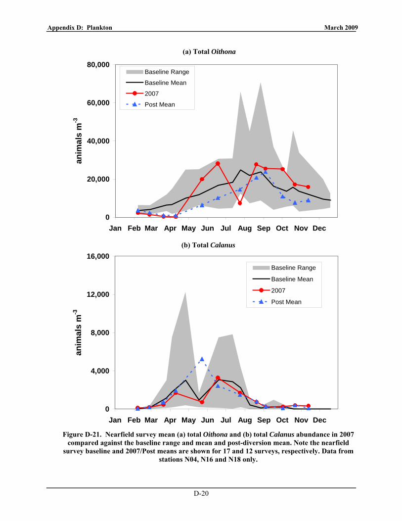
Appendix D: Plankton March 2009
D-20
(a) Total Oithona
0
20,000
40,000
60,000
80,000
Jan Feb Mar Apr May Jun Jul Aug Sep Oct Nov Dec
anim
als
m-3
Baseline Range
Baseline Mean
2007
Post Mean
(b) Total Calanus
0
4,000
8,000
12,000
16,000
Jan Feb Mar Apr May Jun Jul Aug Sep Oct Nov Dec
anim
als
m-3
Baseline Range
Baseline Mean
2007
Post Mean
Figure D-21. Nearfield survey mean (a) total Oithona and (b) total Calanus abundance in 2007
compared against the baseline range and mean and post-diversion mean. Note the nearfield survey baseline and 2007/Post means are shown for 17 and 12 surveys, respectively. Data from
stations N04, N16 and N18 only.

Appendix D: Plankton March 2009
D-21
(a) Total Zooplankton Abundance
0
50,000
100,000
150,000
200,000
250,000
300,000
1992 1993 1994 1995 1996 1997 1998 1999 2000 2001 2002 2003 2004 2005 2006 2007
Ani
mal
s m
-3
Boston Harbor Coastal Nearfield Offshore N. Boundary Cape Cod
(b) Total Zooplankton Long-Term Trend
0
10,000
20,000
30,000
40,000
50,000
60,000
70,000
1990 1995 2000 2005 2010
Tota
l zoo
plan
kton
tre
nd (#
m-3
)
Figure D-22. Time series of total zooplankton abundance by area (a) and the long-term trend (1992- 2007) in total zooplankton abundance derived from time series analysis (b). Long-term
mean levels are also shown (red). Data from stations N04, N16 and N18, only.

Appendix D: Plankton March 2009
D-22
(a) Total Copepods
0
10,000
20,000
30,000
40,000
50,000
1990 1995 2000 2005 2010
Tota
l cop
epod
tren
d (#
m-3
)
(b) Total Copepod Nauplii
0
5,000
10,000
15,000
20,000
1990 1995 2000 2005 2010
Cop
epod
nau
plii
tren
d (#
m-3
)
Figure D-23. Long-term trend (1992- 2007) in (a) total copepod and (b) copepod nauplii
abundance derived from time series analysis. Long-term mean levels are also shown (red). Data from stations N04, N16 and N18, only.

Appendix D: Plankton March 2009
D-23
(a) Oithona similis
0
5,000
10,000
15,000
20,000
1990 1995 2000 2005 2010
Oith
ona
tren
d (#
m-3
)
(b) Calanus finmarchicus
0
500
1,000
1,500
2,000
1990 1995 2000 2005 2010
Cal
anus
finm
arch
icus
tre
nd (#
m-3
)
Figure D-24. Long-term trend (1992- 2007) in (a) Oithona similis and (b) Calanus finmarchicus abundance derived from time series analysis. Long-term mean level is also shown (red). Data
from stations N04, N16 and N18, only.

Massachusetts Water Resources Authority Charlestown Navy Yard
100 First Avenue Boston, MA 02129
(617) 242-6000 http://www.mwra.state.ma.us