water balance modeling of upper blue nile catchments using a top-down approach

Hydrol. Earth Syst. Sci., 15, 2179–2193, 2011www.hydrol-earth-syst-sci.net/15/2179/2011/doi:10.5194/hess-15-2179-2011© Author(s) 2011. CC Attribution 3.0 License.

Hydrology andEarth System

Sciences

Water balance modeling of Upper Blue Nile catchmentsusing a top-down approach

S. Tekleab1,2,3,4, S. Uhlenbrook1,4, Y. Mohamed1,4, H. H. G. Savenije4, M. Temesgen1,5, and J. Wenninger1,4

1UNESCO-IHE Institute for Water Education, P.O. Box 3015, 2601 DA Delft, The Netherlands2Addis Ababa University, Institute for Environment, Water and Development, Addis Ababa University, P.O. Box 1176,Addis Ababa, Ethiopia3Hawassa University, Department of Irrigation and Water Resources Engineering, P.O. Box 5, Hawassa, Ethiopia4Delft University of Technology, Faculty of Civil Engineering and Applied Geosciences, Water Resources section,Stevinweg 1, P.O. Box 5048, 2600 GA Delft, The Netherlands5Addis Ababa University, Department of Civil Engineering, P.O. Box 385, Addis Ababa, Ethiopia

Received: 1 July 2010 – Published in Hydrol. Earth Syst. Sci. Discuss.: 13 September 2010Revised: 4 July 2011 – Accepted: 5 July 2011 – Published: 13 July 2011

Abstract. The water balances of twenty catchments in theUpper Blue Nile basin have been analyzed using a top-downmodeling approach based on Budyko’s hypotheses. The ob-jective of this study is to obtain better understanding of waterbalance dynamics of upper Blue Nile catchments on annualand monthly time scales and on a spatial scale of meso scaleto large scale. The water balance analysis using a Budyko-type curve at annual scale reveals that the aridity index doesnot exert a first order control in most of the catchments. Thisimplies the need to increase model complexity to monthlytime scale to include the effects of seasonal soil moisture dy-namics. The dynamic water balance model used in this studypredicts the direct runoff and other processes based on thelimit concept; i.e. for dry environments since rainfall amountis small, the aridity index approaches to infinity or equiva-lently evaporation approaches rainfall and for wet environ-ments where the rainfall amount is large, the aridity indexapproaches to zero and actual evaporation approaches thepotential evaporation. The uncertainty of model parametershas been assessed using the GLUE (Generalized LikelihoodUncertainty Estimation) methodology. The results show thatthe majority of the parameters are reasonably well identifi-able. However, the baseflow recession constant was poorlyidentifiable. Parameter uncertainty and model structural er-rors could be the reason for the poorly identifiable parame-ter. Moreover, a multi-objective model calibration strategyhas been employed to emphasize the different aspects of thehydrographs on low and high flows.

Correspondence to:S. Tekleab([email protected])

The model has been calibrated and validated against ob-served streamflow time series and it shows good performancefor the twenty study catchments in the upper Blue Nile. Dur-ing the calibration period (1995–2000) the Nash and Sutcliffeefficiency (ENS) for monthly flow prediction varied between0.52 to 0.93 (dominated by high flows), while it varied be-tween 0.32 to 0.90 using logarithms of flow series (indicatingthe goodness of low flow simulations). The model is parsi-monious and it is suggested that the calibrated parameterscould be used after some more regionalization efforts to pre-dict monthly stream flows in ungauged catchments of the Up-per Blue Nile basin, which is the vast majority of catchmentsin that region.

1 Introduction

The Blue Nile river emanates from Lake Tana in Ethiopiaat an elevation of 1780 m a.s.l. Approximately 30 km down-stream of Lake Tana, at the Blue Nile falls, the river falls into a deep gorge and travels about 940 km till the Ethiopian-Sudanese boarder (Conway, 1997). Despite its 60 % ofannual flow contribution to the Nile river (e.g. UNESCO,2004; Conway, 2005), the research in the Blue basin has suf-fered from limited hydrological and climatic data availabil-ity, which hampers an in-depth study of the hydrology of thebasin.

The hydrology of the Upper Blue Nile basin was stud-ied using a simple water balance model (e.g. Johnson andCurtis, 1994; Conway, 1997; Mishra and Hata, 2006; Steen-huis et al., 2009). However, most of these studies were con-ducted on large scale to analyze the flow at the outlet at the

Published by Copernicus Publications on behalf of the European Geosciences Union.

http://creativecommons.org/licenses/by/3.0/

2180 S. Tekleab et al.: Water balance modeling of Upper Blue Nile catchments using a top-down approach

Ethiopian-Sudanese border. An understanding of the pro-cesses at sub-catchment level is generally lacking. Moreover,as a part of model uncertainty and parameter identifiabilitystudies, multi-objective calibration searching for optimal pa-rameter sets towards different objective functions was miss-ing in previous studies. Another limitation is that most of thehydrological studies in the Blue Nile have been conducted inthe Lake Tana sub-basin. For example, the applications of theSWAT model in Lake Tana sub-basins (Setegne et al., 2008,2010). Kebede et al. (2006) studied the water balance of LakeTana and its sensitivity to fluctuations in rainfall. Wale etal. (2009) applied HBV model in the Lake Tana sub basin tostudy ungauded catchment contributions to the Lake Waterbalance.

Uhlenbrook et al. (2010) studied the hydrological dynam-ics and processes of Gilgel Abay and Koga catchments us-ing also the HBV model. Assessments of climate changeimpacts on hydrology of the Gilgel Abay catchment also in-dicate that the catchment is sensitive to climate change es-pecially to changes in rainfall (Abdo et al., 2009). Gebrey-ohannis et al. (2010) studied the relation of forest cover andstreamflow in the headwater Koga catchment through satel-lite imagery and community perception. They reported thatthe effect of deforestation for the past four decades did notshow any significant change in the flow regime.

Assessment of catchment water balance is a pre-requisiteto understand the key processes of the hydrologic cycle.However, the challenge is more distinct in developing coun-tries, where data on climate and runoff is scarce as in the caseof Upper Blue Nile basin. In such cases, a water balancestudy can provide insights into the hydrological behavior ofa catchment and can be used to identify changes in main hy-drological processes (Zhang et al., 1999). In order to ana-lyze the catchment water balance Budyko (1974) developeda framework linking climate to evaporation and runoff from acatchment. He developed an empirical relationship betweenthe ratio of mean annual actual evaporation to mean annualrainfall and mean annual dryness index of the catchment.

The Budyko hypothesis has been widely applied in thecatchments of the former Union of Soviet Socialist Republics(USSR). Similar studies were conducted worldwide usingBudyko’s framework (e.g. Milly, 1994; Koster and Suarez,1999; Sankarasubramania and Vogel, 2002, 2003; Zhang etal., 2004; Potter et al., 2005; Donohue et al., 2007; Ger-rits et al., 2009; Potter and Zhang, 2009; Yang et al., 2009).All these studies improved Budyko framework by includingadditional processes. Zhang et al. (2001, 2008) and Yanget al. (2007) suggested that by assuming negligible storageeffects for long term mean (>5 year) the annual aridity in-dex (8 =E0/P ) controls partitioning of precipitation (P ) toevaporation (E) and runoff (Q). E0 is the potential evap-oration, whileE is actual evaporation. By evaporation wemean all forms of water changes from liquid to vapor, i.e. soiland open water evaporation plus transpiration and intercep-tion evaporation. This is often termed evapotranspiration or

total evaporation in the literature. However, Sankarasubra-mania and Vogel (2002, 2003) argued that the aridity indexis not the only variable controlling the water balance at an-nual time scale and that the evaporation ratio (E/P) is relatedto soil moisture storage as well. Their results improved byincluding a soil moisture storage index, which could be de-rived from the “abcd” watershed model. The abcd watershedmodel is a nonlinear water balance model which uses precip-itation and potential evaporation as input, producing stream-flow as output.

The model has four parametersa, b, c and d. The pa-rameter “a” represents the tendency of runoff to occur be-fore the soil is fully saturated. The parameter “b” is an up-per limit on the sum of evaporation and soil moisture stor-age. The parameter “c” represents the fraction of streamflowwhich, arises from groundwater. The parameter “d” repre-sents the base flow recession constant (Sankarasubramaniaand Vogel; 2002). Besides, they classified catchments in theUS based on the aridity index range of 0–0.33 as humid,0.33–1 as semi-humid, 1–2 as temperate, 2–3 as semi-aridand 3–7 as arid. Milly (1994) showed that the spatial dis-tribution of soil moisture holding capacity and temporal pat-tern of rainfall can affect catchment evaporation, but couldbe of small influence on annual time scale. Obviously, spa-tial and temporal variability of vegetation affects evapora-tion and hence the water balance. Thus, it is more importantto include the soil moisture storage for smaller spatial andtemporal scales (Donohue et al., 2007). Zhang et al. (2004)hypothesized that the plant available water capacity coeffi-cient reflects the effect of vegetation on the water balance.They developed a two parameter model which relates themean annual evaporation to rainfall, potential evaporationand plant available water capacity to quantify the effect oflong term vegetation change on mean annual evaporation (E)in 250 catchments worldwide and found encouraging results.Inspired by the work of Fu (1981), Yang et al. (2007) an-alyzed the spatio-temporal variability of annual evaporationand runoff for 108 arid/semi-arid catchments in China andexplored both regional and inter-annual variability in annualwater balance and confirmed that the Fu (1981) equation canprovide a full picture of the evaporation mechanism at theannual timescale.

The distinct feature of the present study as compared tothe previous study is that, we learned from the data startswith simple annual model in different sub-catchments within the Upper Blue Nile basin based on Budyko frameworkand model complexity is increased to monthly time scale.The monthly water balance model developed by Zhang etal. (2008), which is based on the Budyko hypotheses, hasbeen tested in 250 catchments in Australia with differentrainfall regimes across various geographical region and theyobtained encouraging results. We have applied this model inthe Upper Blue Nile catchments due to its parsimony, onlyhaving four physically meaningful parameters and its ver-satility to predict streamflow and to investigate impacts of

Hydrol. Earth Syst. Sci., 15, 2179–2193, 2011 www.hydrol-earth-syst-sci.net/15/2179/2011/

S. Tekleab et al.: Water balance modeling of Upper Blue Nile catchments using a top-down approach 2181

vegetation cover change on stream flow. Fang et al. (2009)applied the model in Australian and South African catch-ments on a monthly time scale and meso-scale and to largescale to study land cover change impacts on streamflow.

Moreover, in data scares environment like the Upper BlueNile basin, complex models which require more input dataand large number of parameters are not recommended. Themodel used in this study has only four parameters. The mostcommonly used hydrological models which have been ap-plied in the Blue Nile basin are conceptual semi-distributedmodel like the Soil and Water Assessment Tool (SWAT)(more than 20 parameters, many temporal variable) and theconceptual HBV model (Hydrologiska Byrans Vattenbal-ansavdelning) has (12 parameters). They have many moreparameters than the four parameters model used in this study.Therefore, in terms of over parameterization, which is themajor cause of equifinality, the previous models were moreprone to equifinality problem than the model we used in thisstudy.

The objective of this paper is building on the work ofBudyko (1974), Fu (1981), Zhang et al. (2004, 2008) toinvestigate the water balance dynamics of twenty catch-ments in the Upper Blue Nile on temporal scales ofmonthly and annual and spatial scales of meso-scale (catch-ment area between 10–1000 km2) to large scale (catchmentarea> 10 000 km2). Consequently, the basis for predictingwater balance parameters in ungauged basins is laid.

2 Study area and input data

2.1 Study area

The Upper Blue Nile River is located in the highlands ofEthiopia (Fig. 1). The elevation ranges between 489 onthe western side to 4261 m a.s.l. at Mount Ras Dashen inthe north-eastern part. The catchment boundary and thedrainage pattern have been delineated using ArcGIS 9.3with a 90 m resolution digital elevation model of the NASAShuttle Radar Topographic Mission (SRTM) obtained fromthe Consortium for Spatial Information (CGIRCSI) website(http://srtm.csi.cgiar.org).

The climate in the Upper Blue Nile river basin variesfrom humid to semi-arid and it is mainly dominated by lat-itude and altitude. The influence of these factors determinea rich variety of local climates, ranging from hot and aridalong the Ethiopia-Sudan border to temperate at the high-lands and even humid-cold at the mountain peaks in Ethiopia.According to the present study, the mean annual tempera-ture ranges from 13◦C in south eastern parts to 26◦C inthe lower areas of the south western part for the period1995–2004. The Ethiopian National Meteorological Ser-vices Agency (ENMA) defines three seasons in Ethiopia:rainy season (June to September), dry season (October toJanuary) and short rainy season (February to May). The

short rains, originating from the Indian Ocean, are broughtby south-east winds, while the heavy rains in the wet seasonoriginate mainly from the Atlantic Ocean and are related tosouth-west winds (BCEOM, 1999; Seleshi and Zanke, 2004).The study by Camberlin (1997) reported that the monsoonactivity in India is a major cause for summer rainfall variabil-ity in the East African highlands. A recent study by Haile etal. (2009) showed that the variation of rainfall at the sourceof the Blue Nile River in Lake Tana sub-basin is affected byterrain elevation and distance to the center of the Lake. More-over, in their study it is indicated that the amount of nocturnalrainfall (rainfall during the night time) over the Lake shorewas about 75 % of the total rainfall and it is higher than thenocturnal rainfall over the mountainous areas.

The rainfall in the basin has a mono-modal pattern. An-nual rainfall values constructed from eleven gauges rangebetween 1148–1757 mm yr−1 during the period 1900–1998has a mean value of 1421 mm yr−1 and 70 % of it con-centrates between June and September (Conway, 2000).Abtew et al. (2009) studied the spatial and temporal distri-bution of meteorological parameters in the upper Blue Nilebasin. According to their study the mean annual rainfall is1423 mm yr−1 for the period of 1960–1990. The dominantland cover in the basin is rainfed agriculture, i.e. cropland(26 %) and grassland (25 %). Wood and shrub land are minorcompared to the other land cover types (Teferi et al., 2010).The soil type in the basin is dominated by Vertisol and Ni-tisol types (53 %). The Nitisols are deep non swelling claysoils with favorable physical properties like drainage, work-ability and structure, while the Vertisols are characterizedby swelling clay minerals with more unfavorable conditions.The basin geology is characterized by basalt rocks, which arefound in the Ethiopian highlands, while the lowlands mainlycomposed of basement rocks and metamorphic rocks such asgneisses and marbles (ENTRO, 2007).

2.2 Input data

Monthly stream flow time series of 20 rivers covering theperiod 1995–2004 have been collected from the Ministry ofWater Resources Ethiopia, Department of Hydrology. Thequality of the input data has been checked based on com-parison graphs of neighboring stations and also double massanalyses were carried out to check the consistency of thetime series on a monthly basis. The missing data were filledin using regression analysis. Monthly meteorological datafor the same period were obtained from the Ethiopian Na-tional Meteorological Agency (ENMA). The data comprisesprecipitation from 48 stations and temperature from 38 sta-tions. Potential evaporation was computed using Hargreavesmethod with minimum and maximum average monthly tem-perature as input data (Hargreaves and Samani, 1982). Thismethod was selected due to the fact that meteorological datain the region is scarce, which limits the possibility to use dif-ferent methods for the computation of potential evaporation.

www.hydrol-earth-syst-sci.net/15/2179/2011/ Hydrol. Earth Syst. Sci., 15, 2179–2193, 2011

http://srtm.csi.cgiar.org


24

685

686

687

688

689

690

691

692

693

694

695

696

697

698

699

700

701

702

703

704

705

706

707

Fig. 1 Study area; numbers indicate the location of gauging stations of modeled catchments.708

Legend

!( 20 modelled catchments stream gauging stations

Climate stations

Stream gauging stations at Kessie Bridge & Ethiopian-Sudanese border

Rivers

Lake Tana

Sub basins boundary

Fig. 1. Study area; numbers indicate the location of gauging stations of modeled catchments.

However, the Penman-Monteith method, which has been ap-plied successfully in different parts of the world, was com-pared with other methods and is accepted as the preferredmethod for computing potential evaporation from meteoro-logical data (Allen et al., 1998; Zhao et al., 2005). The Har-greaves model was recommended for the computation of po-tential evaporation, if only the maximum and minimum airtemperatures are available (Allen et al., 1998). Hargreavesand Allen (2003) also reported that the results computing themonthly potential evaporation estimates obtained using Har-greaves method were satisfactory. For example Sankarasub-ramania and Vogel (2003) used Hargreaves model to estimatethe monthly potential evaporation in 1337 catchments in US.Table 1 presents basic hydro-meteorological characteristicsof the twenty study catchments.

3 Methodology

3.1 The Budyko framework

Budyko-type curves were developed by many researchers inthe past (Schreiber, 1904; Ol’dekop, 1911; Turc, 1954; Pike,1964; Fu, 1981). The assumptions inherent to the Budykoframework are:

1. Considering a long period of time (τ ≥ 5 years), thestorage variation in catchments may be disregarded(i.e.1S≈ 0).

2. Long term annual evaporation from a catchment is de-termined by rainfall and atmospheric demand. As a re-sult, under very dry conditions, potential evaporation



Table 1. Hydro-meteorological characteristics of the investigatedtwenty upper Blue Nile catchments (1995–2004);P , E0, Q andE

stand for basin precipitation, potential evaporation, discharge andactual evaporation, respectively.

Long term mean annual values(mm yr−1)

Catchment Catchment Area P E0 Q E

number name (km2)

1 Megech 511 1138 1683 421 7172 Rib 1289 1288 1583 349 9393 Gumera 1269 1330 1671 841 4884 Beles 3114 1402 1826 643 7595 Koga 295 1286 1751 606 6796 Gilgel Abay 1659 1724 1719 1043 6817 Gilgel Beles 483 1703 1741 897 8068 Dura 592 2061 1788 1004 10569 Fetam 200 2357 1619 1400 95610 Birr 978 1644 1677 553 109111 Temcha 425 1409 1512 623 78512 Jedeb 277 1449 1454 861 58713 Chemoga 358 1441 1454 461 98014 Robigumero 938 1052 1362 289 76215 Robijida 743 1002 1379 222 78016 Muger 486 1215 1654 480 73517 Guder 512 1734 1744 713 102018 Neshi 327 1654 1416 686 96719 Uke 247 1957 1488 1355 60220 Didessa 9672 1538 1639 334 1204

may exceed precipitation, and actual evaporation ap-proaches precipitation. These relations can be writtenas Q

P→ 0, E

P→ 1, andE0

P→ ∞. Similarly, under very

wet conditions, precipitation exceeds potential evapora-tion, and actual evaporation asymptotically approachesthe potential evaporationE → E0, andE0

P→ 0.

The Budyko (1974) equation can be written as:

E

P=

[φ tanh

(1

φ

) (1 − exp−φ

)]0.5

(1)

The Budyko curve representing the energy and water limitasymptotes are shown in Fig. 2.

3.2 Catchment water balance model at annual timescale

To study catchment water balance hydro-meteorologicalvariables have been prepared for the model as an input.The average precipitation and potential evaporation for eachtwenty catchments have been estimated using thiesen poly-gon method. Figure 1 illustrates the hydro-meteorologicallocation used in this study. Due to scares data availabilitywith many gaps in the time series, only twenty catchmentswith relatively having good quality of streamflow, precipita-tion and temperature measurements were used in this study.

2

26

27

Fig. 2 Budyko curve representing evaporation ratio is a function of aridity index.28 Fig. 2. Budyko curve representing evaporation ratio is a function ofaridity index.

The water balance equation of a catchment at annual timescale can be written as:

dS

dt= P − Q − E (2)

where: P is precipitation (mm yr−1), Q is the total runoff(mm yr−1), i.e. sum of surface runoff, interflow and baseflow,E is actual evaporation (mm yr−1), dS

dtis storage change per

time step (mm yr−1).By assuming storage fluctuations are negligible over long

time scales, i.e.τ ≥ 5 years, Eq. (2) reduces to:

P − Q − E = 0 (3)

Equation (3) is known as a steady state or equilibrium wa-ter balance, which is controlled by available water and at-mospheric demand controlled by available energy (Budyko,1974; Fu, 1981; Zhang et al., 2004, 2008).

Among the different of Budyko-type curves, we usedEq. (4) given by:

E

P= 1 +

E0

P−

[1 +

(E0

P

)w] 1w

(4)

Details of the derivation of this equation can be found in(Zhang et al., 2004). This equation has one annual param-eterw [−], which is a coefficient representing the integratedeffects of catchment characteristics such as vegetation cover,soil properties and catchment topography on the water bal-ance (Zhang et al., 2004). This equation would enable tomodel individual catchments on annual basis. Even though,the results from different Budyko-type curves are not pre-sented here, prediction of annual runoff and evaporation us-ing Eq. (4) was better than the other Budyko-type curves.The selection of Eq. (4) was based on the Nash and Sutcliffeefficiency criterion/measure. Moreover, most of Budyko-type curves including Budyko (1974) do not have calibratedparameters and could not be applied on individual catch-ments (Potter and Zhang, 2009).



The two performance measures Nash and Sutcliffe co-efficient of efficiency (ENS) and root mean squared error(RMSE) were used in the annual model, and are defined asfollows:

ENS = (1) −

n∑i=1

(Qsim,i − Qobs,i

)2

n∑i=1

(Qobs,i − Qobs,i

)2(5)

RMSE =

√√√√1/n ·

n∑i=1

(Qobs,i − Qsim,i

)2 (6)

where Qsim,i is the simulated streamflow at timei[mm yr−1], Qobs,i is the observed streamflow at timei[mm yr−1], n is the number of time steps in the calibra-tion period and the over-bar indicates the mean of observedstreamflow.

3.3 Catchment water balance model at monthly timescale

The dynamic water balance model developed by Zhang etal. (2008) has been used to simulate the monthly stream-flow. The model has four parameters describing direct runoffbehaviorα1 [−], evaporation efficiencyα2 [−], catchmentstorage capacitySmax [mm], and slow flow componentd[1/month]. Zhang et al. (2008) stated that each parametercan be interpreted physically. For example the parameterα1represents catchment rainfall retention efficiency and an in-crease in parameterα1 implies higher rainfall retention andless direct runoff. The maximum soil water storage in theroot zone (Smax) relates to soil and vegetation characteristicsof the catchment. The parameterα2 relates to the evaporationefficiency, a

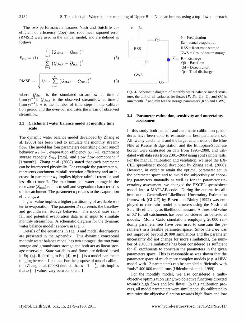
higher value implies a higher partitioning of available wa-ter to evaporation. The parameterd represents the baseflowand groundwater storage behavior. The model uses rain-fall and potential evaporation data as an input to simulatemonthly streamflow. A schematic diagram for the dynamicwater balance model is shown in Fig. 3.

Details of the equations in Fig. 3 and model descriptionsare presented in the Appendix. This dynamic conceptualmonthly water balance model has two storages: the root zonestorage and groundwater storage and both act as linear stor-age reservoirs. State variables and fluxes are defined basedin Eq. (4). Referring to Eq. (4),w [−] is a model parameterranging between 1 and∞. For the purpose of model calibra-tion Zhang et al. (2008) defined thatα = 1−

1w

, this impliesthatα [−] values vary between 0 and 1.

3

29 30 31 32 33 34 35 36 37

38

39

40

41

42

43

Fig. 3 Schematic diagram of monthly water balance model structure; the unit of all 44

variables for fluxes (P, Ea, Qd, Qb and Qt) is mm/month and mm for the storage 45

parameters (RZS and GWS). 46

Qt

Qt = Total dischargeQd = Direct runoffQb = BaseflowR = Richarge

GWS = Ground water storageRZS = Root zone storage

Ea = actual evaporationP = Precipitation

Qd

Qb

Ea

R

GWS

RZS

P

Fig. 3. Schematic diagram of monthly water balance model struc-ture; the unit of all variables for fluxes (P , Ea, Qd, Qb andQt) ismm month−1 and mm for the storage parameters (RZS and GWS).

3.4 Parameter estimation, sensitivity and uncertaintyassessment

In this study both manual and automatic calibration proce-dures have been done to estimate the best parameters set.All twenty catchments and the larger catchments of the BlueNile at Kessie Bridge station and the Ethiopian-Sudaneseborder were calibrated on data from 1995–2000, and vali-dated with data sets from 2001–2004 using split sample tests.For the manual calibration and validation, we used the EX-CEL spreadsheet model developed by Zhang et al. (2008).However, in order to attain the optimal parameter set inthe parameter space and to avoid the subjectivity of choos-ing parameters manually as well as for the parameter un-certainty assessment, we changed the EXCEL spreadsheetmodel into a MATLAB code. During the automatic cali-bration the Generalized Likelihood Uncertainty Estimationframework (GLUE) by Beven and Binley (1992) was em-ployed to constrain model parameters using the Nash andSutcliffe efficiency as likelihood measure. A threshold valueof 0.7 for all catchments has been considered for behavioralmodels. Monte Carlo simulations employing 20 000 ran-domly parameter sets have been used to constrain the pa-rameters in a feasible parameter space. Since theENS wasnot improved beyond 20 000 simulations and the parameteruncertainty did not change for more simulations, the num-ber of 20 000 simulations has been considered as sufficientfor all catchments to constrain the parameters in the givenparameters space. This is reasonable as was shown that theparameter space of much more complex models (e.g. a HBVmodel with 12 parameters) can be sampled sufficiently with“only” 400 000 model runs (Uhlenbrook et al., 1999).

For the monthly model, we also considered a multi-objective optimization using two objective functions directedtowards high flows and low flows. In this calibration pro-cess, all model parameters were simultaneously calibrated tominimize the objective function towards high flows and low



flows. The concept of Pareto optimality is based on the no-tion of domination. It is used to solve the multi-objectiveoptimization and derive Pareto-optimal parameter sets (Feni-cia et al., 2007). All Pareto-optimal solutions are not dom-inated by the others. Mapping the Pareto-optimal solutionsin a feasible parameter space produce Pareto-optimal front,this consists of more than one solution. Past research pointedout that calibration based on one single objective functionoften results in unrealistic representation of the hydrologi-cal system behavior. This means, the information content ofthe data is not fully explained in a single objective function(Gupta et al., 1998; Fenicia et al., 2007). In a monthly modelthe following evaluation criteria were used in this study.

FHF =

n∑i=1

(Qsim,i − Qobs,i

)2

n∑i=1

(Qobs,i − Qobs

)2(7)

FLF =

n∑i=1

[ln

(Qsim,i

)− ln

(Qobs,i

)]2

n∑i=1

[ln

(Qobs,i

)− ln

(Qobs

)]2(8)

whereQsim,i [mm month−1] is the simulated streamflow attime i, Qobs,i [mm month−1] is the observed streamflow attime i, n is the number of time steps in the calibration periodand the over-bar indicates the mean of observed streamflow.The objective functionFHF was selected to minimize the er-rors during high flows (same formula asENS), andFLF useslogarithmic values of streamflow and improves the assess-ment of the low flows.

4 Results and discussions

4.1 Annual water balance

The annual water balance has been computed for the twentycatchments of the Upper Blue Nile basin with the assumptionthat evaporation can be estimated from water availability andatmospheric demand. Among the different Budyko’s typecurves, which were reported by Potter and Zhang (2009),Eq. (4) has been applied to computeE/P for the twenty catch-ments. The selection of this equation was based on the simu-lation results from each catchment evaluated using Nash andSutcliffe efficiency criteria. The predicted annual streamflowand evaporation results are given in Table 2. In most of thesecatchments, Eq. (4) could not predict the annual evaporationand stream flow adequately.

The poor accuracy of the prediction is related to the ef-fect of neglecting soil water storage (assuming dS/dt = 0)and other error sources could influence the results as well,e.g. the uncertainty of catchment rainfall and the estima-tion of potential evaporation, seasonality of rainfall, and

Table 2. Model performance using Eq. (4) for annual runoff andannual evaporation during the period (1995–2004).

Performance measure Runoff Evaporation

min max min max

ENS [−] −2.37 0.84 −0.39 0.73RMSE (mm yr−1) 62.50 298.30 68.10 279.40

non-stationary conditions of the catchment itself (e.g. landuse/cover change). Furthermore, the year to year variabilityof rainfall depth could be the reason for the poor performanceof the model. However, studying the effects of such factorson model simulation at annual time scale was not the objec-tive of this study and needs further research.

Figure 4 illustrates the application of Eq. (4) to predict theregional long term annual mean water balance (1995–2004)of the twenty catchments.

It can be seen that the aridity index varies from 0.7 to 1.5,and some catchments represent a semi-humid environment,when the aridity index less than 1.0 and others are drier withan aridity index greater than 1.0. Based on the aridity index,the Upper Blue Nile catchments can be classified as semi-arid to semi-humid and temperate.

Considering all twenty catchments, the regional mean an-nual water balance were adequately predicted by Eq. (4) witha single model parameter (w = 1.8) the model gave reason-able good performance with a Nash and Sutcliffe efficiencyof (ENS) 0.70 and a root mean squared error of 177 mm yr−1.The results of predicting the regional mean annual water bal-ance using Eq. (4) in this study is in agreement with theresearch work in different parts of the world (e.g. Yang etal., 2007; Zhang et al., 2008; Potter et al., 2005; Potter andZhang, 2009).

Furthermore, as it can be seen in Fig. 4 that differentgroups of catchments follow a unique curve with an inde-pendentw [−] value. Thus, the results depicts that catch-ment evaporation ratio varies from catchment to catchment.Based on evaporation ratio catchments are categorized in tothree groups, what suggests that each group has differentcharacteristics. Study by Potter and Zhang (2009) classi-fied catchments in Australia based on rainfall regime as win-ter dominant, summer dominant, seasonal and non-seasonalcatchments. Yang et al. (2007) also classified 108 arid tosemi-arid catchments in China based on the patterns whichthe catchments follow on the Fu curve. Moreover, Zhang etal. (2004) categorized catchments in Australia based on veg-etation cover as forested and grass land catchments with ahigher parameterw values for forested catchments and lowervalues of the parameterw for grass covered catchments.

Table 3 presents goodness-of-fit statistics as recom-mended by Legates and McCabe (1999) for each group of



4

47 48 49 50

Fig. 4 Mean annual evaporation ratio (E

P) as a function of Aridity Index (

P

E0 ) for different 51

values of w using Fu (1981) curve. 52

Fig. 4. Mean annual evaporation ratio (E

P) as a function of Aridity Index (E0

P) for different values ofw using Fu (1981) curve.

Table 3. Average goodness-of-fit statistics Nash and Sutcliffe effi-ciency (ENS) and root mean squared error (RMSE) for predictionof regional long term mean annual streamflow using Fu’s curve.

ENS (−) RMSE Calibrated(mm yr−1) parameter “w”

All catchments 0.70 177.51 1.8Group-1 catchments1 0.87 76.36 1.5Group-2 catchments2 0.97 57.22 1.9Group-3 catchments3 0.85 58.23 2.5

1 Gilegl Abay, Koga, Gumera, Jedeb, Uke, Gilgel Beles and Beles.2 Fetam, Dura, Guder, Muger, Temcha and Megech.3 Neshi, Chemoga, Birr, Rib, Robi Gumero, Robi Jida and Didessa.

catchments. The Nash and Sutcliffe efficiency (ENS) androot mean squared error (RMSE) show that the long termaverage annual streamflow for each group of catchment waspredicted adequately using Eq. (4).

From the results of modeled individual catchments, it isnoted that the calibrated parameterw ranges between 1.4and 3.6. This may suggest that the Upper Blue Nile catch-ments under consideration exhibit different catchment char-acteristics. Zhang et al. (2004) pointed out that smaller val-ues ofw are associated with high rainfall intensity, season-ality, steep slope and lower plant available soil water stor-age capacity. However, it is difficult to represent these char-acteristics explicitly in a simple model (Zhang et al., 2004;

Yang et al., 2007). Typically the result of the analysis fromgroup-1 catchments in our study indicates that a larger frac-tion of precipitation becomes surface runoff, which resultsin lower evaporation ratios for this group compared to theother groups. Besides, the computed runoff coefficients forgroup-1 catchments ranges between 0.5–0.7 suggest that sur-face runoff was dominant in these catchments. The catch-ments in Group-2 have higher evaporation ratio and lowerrunoff coefficients (0.37–0.47) than Group-1. But Group-3catchments have higher evaporation ratios, lower runoff po-tential and hence have lower values of the runoff coefficients(0.21–0.33).

It is also noted that the parameterw summarizes integratedcatchment characteristics such as land cover, geology, soilproperties and topography. It is not possible to fully explainthe effects ofw for each group of catchment due to the lackof detail data of physiographic characteristics in the region.

4.2 Modeling streamflow at monthly time scale

Modeling at finer time scale (monthly and daily) requiresthe inclusion of soil moisture dynamics to accurately esti-mate the water balance. In a top down modeling approach,model complexity has to be increased when deficiencies ofthe model structure in representing the catchment behavioris encountered (Jothityangkoon et al., 2001; Atkinson et al.,2002; Montanari et al., 2006; Zhang et al., 2008). Therefore,a somewhat more complex model structure has been appliedthat is still very simple and has four parameters (see Fig. 3).



5

53 54

55 56 57 58 59

60 61 62 63

64 65 66 67 68 69 70 71 72 73 74 75 76 77 78 79 80 81 82 83 84 85 86 87 88 89 90 91 92 93 94 95 96 97

5

53 54

55 56 57 58 59

60 61 62 63

64 65 66 67 68 69 70 71 72 73 74 75 76 77 78 79 80 81 82 83 84 85 86 87 88 89 90 91 92 93 94 95 96 97

6

98

99 100 101 102 103

104

105

106

107

108

109

110

111

112

113

114

115

116

117

118

119

Fig. 5 Observed and simulated streamflows during calibration period (1995-2000) for 120

selected catchments. 121

6

98

99 100 101 102 103

104

105

106

107

108

109

110

111

112

113

114

115

116

117

118

119

Fig. 5 Observed and simulated streamflows during calibration period (1995-2000) for 120

selected catchments. 121

Fig. 5. Observed and simulated streamflows during calibration period (1995–2000) for selected catchments.



and erosion for the Abay Blue Nile with a simple model, Wiley Inter-Science,

submitted, 2009. update?

It is now updated as:

Steenhuis, T., Collick, A., Easton, Z., Leggesse, E., Bayabil, H.,White, E., Awulachew,

S., Adgo, E., and Ahmed, A.: Predicting discharge and sediment for the Abay

(Blue Nile) with a simple model, Hydrol. Process., 23, 3728–3737, 2009.

7. On page 10 Fig.6. is now modified as below. Nme of the catchment and title on axeses

are now a little bet visible than previous. Would you please use this updated fig?

6.

Fig. 6. GLUE dotty plots of selected meso-scale catchments and Blue Nile at larger scale

at Kessie Bridge and Ethiopian-Sudanese border. Fig. 6. GLUE dotty plots of selected meso-scale catchments and Blue Nile at larger scale at Kessie Bridge and Ethiopian-Sudanese border.

The monthly streamflows were calibrated for the period1995–2000 and validated for the period 2001–2004. In themanual calibration and validation the Nash and Sutcliffe co-efficient efficiency was used as leading performance mea-sure. The main objective of calibration is finding the opti-mal parameter set that maximizes or minimizes the objectivefunction for the intended purposes. In the parameter identi-fication process, different parameter sets were sampled ran-domly from a priori feasible parameter space as shown inTable 4, which is in agreement with the literature (Zhang etal., 2008) and manual calibration in this study.

The dynamic water balance model was calibrated andvalidated for the twenty catchments and also at the twolarger catchments with gauging stations at Kessie Bridgestation (64 252 km2) and at the Ethiopian-Sudanese border(173 686 km2) to test the ability of the model at large spa-tial scale. During calibration Nash and Sutcliffe coeffi-cients were obtained in the range of 0.52–0.95 (dominated byhigh flows) and 0.33–0.93 using logarithmic discharge valueswhen calculatingENS (dominated by low flows).

Similarly, during the validation period Nash and Sutcliffeefficiencies were obtained in the range of 0.55–0.95 dur-ing high flows and 0.12–0.91 during low flows. The model

Table 4. Ranges of parameter values for the catchments modeled inthe Upper Blue Nile basin based on manual calibration and Zhanget al. (2008).

Lower/upper bound

Catchment Smax [mm] α1 [−] α2 [−] d [1/month]

Gilgel Abay, Koga, Birr, 100–600 0–1 0–1 0–1Fetam, Neshi

Dura, Gilgel Beles, 100–600 0.1–0.75 0.1–0.75 0–1Gumera, Megech, Rib,Robigumero, Robijida,Didessa

Chemoga, Beles, Guder 100–600 0.1–0.85 0.1–0.85 0–1

Muger, Temcha, Uke, 100–600 0–0.9 0–0.8 0–1Jedeb

results reveal that during calibration, the model gave reason-able results in most of the catchments including the simu-lation at larger scale at Kessie Bridge station (ENS = 0.95)and at the Ethiopian-Sudanese border (ENS = 0.93). How-ever, during the validation period in some catchments the



low flows were not captured well by the model. Though alot of uncertainties in model structure and model parameterswere common in hydrological models, it is speculated thatthe likely reason for poor efficiency values in some catch-ments were more related to the uncertainties in the input datasets. Figure 5 shows observed and predicted streamflowsusing automatic calibration for selected meso-scale catch-ments and the larger scale results at Kessie Bridge stationand Ethiopian-Sudanese border.

The optimal parameter values obtained using GLUEframework together with parameters obtained manually arepresented in Table 5.

It is clearly demonstrated that the parameter values differand the performance of the model improved using a GLUEframework. The parameterα1 in majority of the catchmentsshows that the rainfall amount retained by the catchments isnot significant, thus fast runoff generation process are dom-inant in the studied catchments. This high responsivenessis also in line with field observations where the formationof surface runoff (and significant soil erosion) can be ob-served. The values of evaporation efficiency parameterα2are higher in some catchments which implies higher parti-tioning of available water into evaporation. The higher evap-oration efficiency parameter in these catchments reveals thatthe catchments were relatively having high forest cover andevaporation was dominant and less surface runoff was gener-ated in these catchments. The dotty plots used to map the pa-rameter value and their objective function values as a meansof assessing the identifiability of parameters are shown inFig. 6.

It can be seen that most of the parameters in the UpperBlue Nile catchments are reasonably well identifiable; how-ever, the recession constantd exhibit poor identifiability inthe majority of the catchments. It is speculated that parame-ter uncertainty and model structural errors could be the rea-son for the poorly identifiable groundwater parameter.

Furthermore, the model performances in the objectivefunction space of Pareto-optimal fronts resulting from themonthly water balance model were investigated (see Fig. 7).

From multi-objective optimization point of view, thePareto-optimal solutions are all equally important to achievea better model simulation. The Pareto based approach is alsoimportant to compare different model structures in such away that model improvement can be attained as the Pareto-optimal front progressively moves towards the origin of theobjective function space (Fenicia et al., 2007; Wang et al.,2007). From Fig. 7 it can be noticed that for different catch-ments the Pareto-optimal set of solutions approach to the ori-gin differently. It is demonstrated that the model structureperforms better at the larger scale than for the meso-scalecatchments. As the objective function values get closer tothe origin, the chosen model structure represents the hydro-logic system better.

8. On page 11 Right column Fig.7. I made few changes on the title of axis and legend

The font Arial is now changed in to Times new Roman. So would you please use the

updated fig below?

Fig. 7. Pareto-optimal fronts of parameter sets at different meso-scale

catchments and Blue Nile at the larger scale based on the selected

objective functions [low flows (FLF), high flows (FHF)].

I could not find any other correction in the proof reading. Looking forward to hear about

the correction is sufficient or not.

With Kind Regards,

Sirak Tekleab

Fig. 7. Pareto-optimal fronts of parameter sets at different meso-scale catchments and Blue Nile at the larger scale based on the se-lected objective functions [low flows (FLF), high flows (FHF)].

5 Conclusions

The Upper Blue Nile catchment water balance has been ana-lyzed at different temporal and spatial scales using Budyko’sframework. The analysis included water balance at mean an-nual, annual and monthly time scales for meso to large scalecatchments. A Budyko-type curve (Fu, 1981) was applied toexplore the first order control based on available water andenergy over mean annual and annual time scales. The resultsdemonstrated that predictions are not good in the majority ofthe catchments at annual time scale. This implies that at an-nual scale the water balance is not dominated only by precipi-tation and potential evaporation. Thus, increased model com-plexity to monthly time scale is necessary for a realistic simu-lation of the catchment water balance by including the effectsof soil moisture dynamics. Parameters were identified usingthe Generalized Likelihood Uncertainty Estimation (GLUE)framework in addition to manual calibration and the resultsshowed that most of the parameters are identifiable and themodel is capable of simulating the observed streamflow quitewell. The applicability of this model was tested earlier in 250catchments in Australia with different rainfall regimes acrossdifferent geographical regions and results were encouraging(Zhang et al., 2008; Fang et al., 2009). Similarly, in the Up-per Blue Nile case, the model performs well in simulating themonthly streamflow of the twenty investigated catchments.

With only four parameters the simple model has the ad-vantage of minimal equifinality. Despite the uncertainties ininput data, parameters and model structure, the model givesreasonable results for the Upper Blue Nile catchments. How-ever, it is suggested that on annual time scale the reasonsfor poor model efficiencies in majority of the catchments,which followed distinct Budyko-type curves, needs furtherresearch. It is recommended that future work should focus



Table 5. Comparison of automatic (GLUE) single objective and manually calibrated parameters andENS values of the twenty selectedUpper Blue Nile catchments during the period 1995–2000.

Catchment Optimized parameters (GLUE) Manually calibrated parameters

Smax [mm] α1 [−] α2 [−] d [1/month] ENS [−] Smax [mm] α1 [−] α2 [−] d [1/month] ENS [−]

Beles 538.09 0.46 0.53 0.96 0.71 365.00 0.50 0.52 0.85 0.70Birr 253.62 0.76 0.92 0.87 0.93 330.00 0.57 0.62 0.91 0.82Chemoga 216.40 0.66 0.81 0.89 0.93 260.00 0.60 0.63 0.90 0.90Didessa 590.02 0.58 0.85 0.48 0.52 520.00 0.64 0.86 0.23 0.52Dura 331.56 0.65 0.63 0.94 0.92 360.00 0.63 0.60 0.86 0.91Fetam 420.89 0.56 0.50 0.99 0.89 280.00 0.52 0.67 0.35 0.81Gilgel Abay 349.30 0.71 0.88 0.12 0.82 390.00 0.60 0.86 0.60 0.81Gilgel Beles 280.03 0.57 0.35 0.98 0.91 280.00 0.55 0.47 0.90 0.89Guder 306.01 0.83 0.45 0.94 0.72 390.00 0.67 0.41 0.85 0.71Gumera 230.82 0.68 0.39 1.00 0.73 350.00 0.47 0.41 0.89 0.72Jedeb 315.96 0.58 0.43 0.93 0.79 260.00 0.58 0.41 0.75 0.78Koga 200.14 0.64 0.46 0.51 0.79 240.00 0.60 0.48 0.60 0.79Megech 313.58 0.55 0.61 0.98 0.81 390.00 0.55 0.62 0.78 0.78Muger 190.52 0.79 0.60 0.97 0.88 210.00 0.63 0.60 0.85 0.84Neshi 397.90 0.79 0.82 0.93 0.80 380.00 0.66 0.64 0.75 0.75Rib 558.43 0.52 0.72 0.99 0.82 370.00 0.63 0.73 0.60 0.76Robigumero 512.88 0.53 0.73 0.02 0.74 500.00 0.50 0.75 0.65 0.73Robijida 243.61 0.69 0.75 0.02 0.91 420.00 0.52 0.78 0.90 0.86Temcha 190.80 0.66 0.63 0.99 0.83 200.00 0.62 0.60 0.80 0.82Uke 441.60 0.70 0.33 0.74 0.82 430.00 0.67 0.33 0.70 0.82

Blue Nile at 268.25 0.70 0.77 0.53 0.95Kessie Bridge

Upper Blue Nile at 439.37 0.76 0.74 0.39 0.93the border to Sudan

on the regionalization of the optimal parameter sets fromthe monthly model presented in this paper for prediction ofstreamflow in ungauged catchments in the Upper Blue Nilebasin.

Appendix A

Details of equation used in the model structure

Figure 3 illustrates the model structure of the dynamicmonthly water balance model. RainfallP(t) at time steptpartitions into direct runoffQd(t) andX(t). X(t) is a lumpedwater balance component known as catchment rainfall reten-tion which consists of the amount of retained water for catch-ment water storage dS/dt , E(t) and rechargeR(t).

P(t) = Qd(t) + X(t) (A1)

whereP(t), andQd(t) are monthly rainfall and direct runoff,respectively. The units of all fluxes are mm month−1.

Analogous to Budyko’s hypothesis, Zhang et al. (2008)defined the demand limit forX(t) to be the sum of dS/dt

and potential evaporation (E0), which is termed asX0(t) andthe supply limit asP(t). If the sum of available storage ca-pacity and potential evaporation is very large as compared

to the supply, thenX(t) approachesP(t) whereas if thesum of available storage capacity and potential evaporationis smaller than the supply,X(t) approachesX0(t). This pos-tulate can be written as:

X(t)

P (t)→ 1, as

X0(t)

P (t)→ ∞ for very dry conditions (A2)

X(t) → X0(t), asX0(t)

P (t)→ 0 for very wet conditions(A3)

The catchment rainfall retention can be expressed as:

X(t) =

{P(t) F

[(X0(t)P (t)

), α1

], P (t) 6= 0

0, P (t) = 0(A4)

whereF [−] is the Fu-curve Eq. (4) andα1 is the retentionefficiency, whereby largerα1 values result in more rainfallretention and less direct runoff.

From Eqs. (A1) and (A4) the direct runoff is calculated as:

Qd = P(t) − X(t) (A5)

The water availabilityW(t) for partitioning can be computedas:

W(t) = E(t) + S(t) + R(t) (A6)



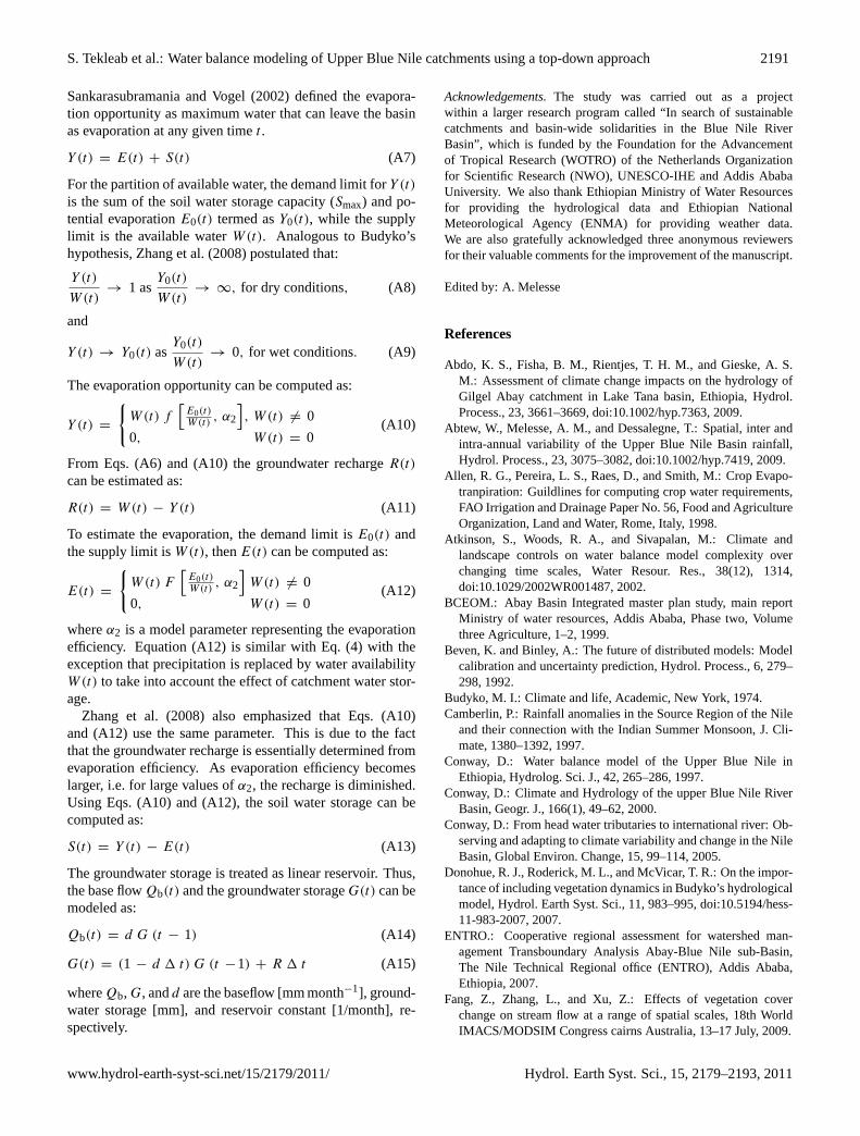
Sankarasubramania and Vogel (2002) defined the evapora-tion opportunity as maximum water that can leave the basinas evaporation at any given timet .

Y (t) = E(t) + S(t) (A7)

For the partition of available water, the demand limit forY (t)

is the sum of the soil water storage capacity (Smax) and po-tential evaporationE0(t) termed asY0(t), while the supplylimit is the available waterW(t). Analogous to Budyko’shypothesis, Zhang et al. (2008) postulated that:

Y (t)

W(t)→ 1 as

Y0(t)

W(t)→ ∞, for dry conditions, (A8)

and

Y (t) → Y0(t) asY0(t)

W(t)→ 0, for wet conditions. (A9)

The evaporation opportunity can be computed as:

Y (t) =

{W(t) f

[E0(t)W(t)

, α2

], W(t) 6= 0

0, W(t) = 0(A10)

From Eqs. (A6) and (A10) the groundwater rechargeR(t)

can be estimated as:

R(t) = W(t) − Y (t) (A11)

To estimate the evaporation, the demand limit isE0(t) andthe supply limit isW(t), thenE(t) can be computed as:

E(t) =

{W(t) F

[E0(t)W(t)

, α2

]W(t) 6= 0

0, W(t) = 0(A12)

whereα2 is a model parameter representing the evaporationefficiency. Equation (A12) is similar with Eq. (4) with theexception that precipitation is replaced by water availabilityW(t) to take into account the effect of catchment water stor-age.

Zhang et al. (2008) also emphasized that Eqs. (A10)and (A12) use the same parameter. This is due to the factthat the groundwater recharge is essentially determined fromevaporation efficiency. As evaporation efficiency becomeslarger, i.e. for large values ofα2, the recharge is diminished.Using Eqs. (A10) and (A12), the soil water storage can becomputed as:

S(t) = Y (t) − E(t) (A13)

The groundwater storage is treated as linear reservoir. Thus,the base flowQb(t) and the groundwater storageG(t) can bemodeled as:

Qb(t) = d G (t − 1) (A14)

G(t) = (1 − d 1 t) G (t −1) + R 1 t (A15)

whereQb, G, andd are the baseflow [mm month−1], ground-water storage [mm], and reservoir constant [1/month], re-spectively.

Acknowledgements.The study was carried out as a projectwithin a larger research program called “In search of sustainablecatchments and basin-wide solidarities in the Blue Nile RiverBasin”, which is funded by the Foundation for the Advancementof Tropical Research (WOTRO) of the Netherlands Organizationfor Scientific Research (NWO), UNESCO-IHE and Addis AbabaUniversity. We also thank Ethiopian Ministry of Water Resourcesfor providing the hydrological data and Ethiopian NationalMeteorological Agency (ENMA) for providing weather data.We are also gratefully acknowledged three anonymous reviewersfor their valuable comments for the improvement of the manuscript.

Edited by: A. Melesse

References

Abdo, K. S., Fisha, B. M., Rientjes, T. H. M., and Gieske, A. S.M.: Assessment of climate change impacts on the hydrology ofGilgel Abay catchment in Lake Tana basin, Ethiopia, Hydrol.Process., 23, 3661–3669,doi:10.1002/hyp.7363, 2009.

Abtew, W., Melesse, A. M., and Dessalegne, T.: Spatial, inter andintra-annual variability of the Upper Blue Nile Basin rainfall,Hydrol. Process., 23, 3075–3082,doi:10.1002/hyp.7419, 2009.

Allen, R. G., Pereira, L. S., Raes, D., and Smith, M.: Crop Evapo-tranpiration: Guildlines for computing crop water requirements,FAO Irrigation and Drainage Paper No. 56, Food and AgricultureOrganization, Land and Water, Rome, Italy, 1998.

Atkinson, S., Woods, R. A., and Sivapalan, M.: Climate andlandscape controls on water balance model complexity overchanging time scales, Water Resour. Res., 38(12), 1314,doi:10.1029/2002WR001487, 2002.

BCEOM.: Abay Basin Integrated master plan study, main reportMinistry of water resources, Addis Ababa, Phase two, Volumethree Agriculture, 1–2, 1999.

Beven, K. and Binley, A.: The future of distributed models: Modelcalibration and uncertainty prediction, Hydrol. Process., 6, 279–298, 1992.

Budyko, M. I.: Climate and life, Academic, New York, 1974.Camberlin, P.: Rainfall anomalies in the Source Region of the Nile

and their connection with the Indian Summer Monsoon, J. Cli-mate, 1380–1392, 1997.

Conway, D.: Water balance model of the Upper Blue Nile inEthiopia, Hydrolog. Sci. J., 42, 265–286, 1997.

Conway, D.: Climate and Hydrology of the upper Blue Nile RiverBasin, Geogr. J., 166(1), 49–62, 2000.

Conway, D.: From head water tributaries to international river: Ob-serving and adapting to climate variability and change in the NileBasin, Global Environ. Change, 15, 99–114, 2005.

Donohue, R. J., Roderick, M. L., and McVicar, T. R.: On the impor-tance of including vegetation dynamics in Budyko’s hydrologicalmodel, Hydrol. Earth Syst. Sci., 11, 983–995,doi:10.5194/hess-11-983-2007, 2007.

ENTRO.: Cooperative regional assessment for watershed man-agement Transboundary Analysis Abay-Blue Nile sub-Basin,The Nile Technical Regional office (ENTRO), Addis Ababa,Ethiopia, 2007.

Fang, Z., Zhang, L., and Xu, Z.: Effects of vegetation coverchange on stream flow at a range of spatial scales, 18th WorldIMACS/MODSIM Congress cairns Australia, 13–17 July, 2009.


http://dx.doi.org/10.1002/hyp.7363

http://dx.doi.org/10.1002/hyp.7419

http://dx.doi.org/10.1029/2002WR001487

http://dx.doi.org/10.5194/hess-11-983-2007



Fenicia, F., Savenije, H. H. G., Matgen, P., and Pfister,L.: A comparison of alternative multi objective calibrationstrategies for hydrological modeling, Water Res., 43, 3434,doi:10.1029/2006WR005098, 2007.

Fu, B. P.: On the calculation of the evaporation from land surface,Sci. Atmos. Sin., 5(1), 23–31, 1981.

Gebreyohannis, S. G., Taye, A., and Bishop, K.: Forest cover andstream flow in a headwater of the Blue Nile: complementing ob-servational data analysis with community perception, Ambio, 39,284–294,doi:10.1007/s13280-010-0047-y, 2010.

Gerrits, A. M. J., Savenije, H. H. G., Veling, E. J. M., and Pfis-ter, L.: Analytical derivation of the Budyko Curve based on rain-fall characterstics and a simple evaporation model, Water Resour.Res., 45, W04403,doi:10.1029/2008WR007308, 2009.

Gupta, H. V., Sorooshian, S., and Yapo, P. O.: Toward improved cal-ibration of hydrologic models: Multiple and non-commensurablemeasures of information, Water Resour. Res., 34(4), 751–764,1998.

Haile, A. T., Rientjes, T. H., Gieske, M., and GebreMichael, M.:Rainfall variability over mountainous and adjacent Lake areas:the case of Lake Tana basin at the source of the Blue Nile River,J. Appl. Meteorol. Clim., 48, 1696–1717, 2009.

Hargreaves, G. H. and Allen, R. G.: History and Evaluation ofHargreaves Evapotranspiration Equation, J. Irrig. Drain. Eng.-ASCE, 129(1), 53–63, 2003.

Hargreaves, G. H. and Samani, Z. A.: Estimating potential evapo-ration. J. Irrig. Drain. Eng.-ASCE, 108(3), 225–230, 1982.

Johnson, P. A. and Curtis, P. D.: Water Balance of Blue Nile RiverBasin in Ethiopia, J. Irrig. Drain. Eng.-ASCE, 120(3), 573–590,1994.

Jothityangkoon, C., Sivapalan, M., and Farmer, D. L.: Process con-trol of water balance variability in a large semi-arid catchmentdown ward approach to hydrological model development, J. Hy-drol., 254(1–4), 174–198, 2001.

Kebede, S., Travi, Y., Alemayehu, T., and Marc, V.: Water balanceof Lake Tana and its sensitivity to fluctuations in rainfall, BlueNile basin, Ethiopia, J. Hydrol., 316, 233–247, 2006.

Koster, R. D. and Suarez, M. J.: A simple frame work for exam-ining the inter annual variability land surface moisture fluxes, J.Climate, 12, 1911–1917. 1999.

Legates, D. R. and McCabe, G. J.: Evaluating the use of “goodness-of- fit” measures in hydrologic and hydroclimatic model valida-tion, Water Resour. Res., 35, 233–241, 1999.

Milly, P. C. D.: Climate, Soil water storage, and the average annualwater balance, Water Resour. Res., 30(7), 2143–2156, 1994.

Mishra, A. and Hata, T.: A Grid based runoff generation and flowrouting model for the upper Blue Nile Basin, Hydrolog. Sci. J.,51(2), 191–205, 2006.

Montanari, L., Sivapalan, M., and Montanari, A.: Investigation ofdominant hydrological processes in a tropical catchment in amonsoonal climate via the downward approach, Hydrol. EarthSyst. Sci., 10, 769–782,doi:10.5194/hess-10-769-2006, 2006.

Ol’dekop, E. M.: On evaporation from the surface of river basins,Transactions on Meteorological Observations, Lur-evskogo,Univ. of Tartu, Tartu, Estonia, 1911.

Pike, J. G.: The estimation of annual runoff from meteorologicaldata in a tropical climate, J. Hydrol., 2, 116–123, 1964.

Potter, N. J., Zhang, L., Milly, P. C. D., McMahon, T. A., and Jake-man, A. J.: Effects of rainfall seasonality and soil moisture ca-pacity on mean annual water balance for Australian catchments,Water Resour. Res., 41, W06007,doi:10.1029/2004WR003697,2005.

Potter, N. J. and Zhang, L.: Inter annual variability of catchmentwater balance in Australia, J. Hydrol., 369, 120-129, 2009.

Sankarasubramania, A. and Vogel, R. M.: Annaual Hydrocli-matology of United States, Water Resour. Res., 38(6), 1083,doi:10.1029/2001WR000619, 2002.

Sankarasubramania, A. and Vogel, R. M.: Hydroclimatology ofthe contential United States, Geophys. Res. Lett., 30, 1363,doi:10.1029/2002GL015937, 2003.

Schreiber, P.:Uber die Beziehungen zwischen dem Niederschlagund der Wasserfuhrung der Flusse in Mitteleuropa, Meteorol. Z.,21, 441–452, 1904.

Seleshi, Y. and Zanke, U.: Recent change in rainfall and rainy daysin Ethiopia. International Journal of climatology, Int. J. Clima-tol., 24, 973–983,doi:10.1002/joc.1052, 2004.

Setegne, S. G., Srinivasan, R., and Dargahi, B.: Hydrological Mod-elling in the Lake Tana Basin, Ethiopia using SWAT model, OpenHydrol. J., 2, 24–40, 2008.

Setegne, S. G., Srinivasan, R., Melesse, A. M., and Dargahi, B.:SWAT model application and prediction uncertainty analysis inthe Lake Tana Basin, Ethiopia, Hydrol. Process., 24, 357–367,2010.

Steenhuis, T., Collick, A., Easton, Z., Leggesse, E., Bayabil, H.,White, E., Awulachew, S., Adgo, E., and Ahmed, A.: Predictingdischarge and sediment for the Abay (Blue Nile) with a simplemodel, Hydrol. Process., 23, 3728-3737, 2009.

Teferi, E., Uhlenbrook, S., Bewket, W., Wenninger, J., and Simane,B.: The use of remote sensing to quantify wetland loss in theChoke Mountain range, Upper Blue Nile basin, Ethiopia, Hy-drol. Earth Syst. Sci., 14, 2415–2428,doi:10.5194/hess-14-2415-2010, 2010.

Turc, L.: Le bilan d’eau des sols Relation entre la precipitationl’evapporation et l’ecoulement, Ann. Agron., 5, 491–569, 1954.

Uhlenbrook, S., Seibert, J., Leibundgut, Ch., and Rodhe, A.: Pre-diction uncertainty of conceptual rainfall-runoff models causedby problems to identify model parameters and structure, Hy-drolog. Sci. J., 44(5), 279–299, 1999.

Uhlenbrook, S., Mohamed, Y., and Gragne, A. S.: Analyzing catch-ment behavior through catchment modeling in the Gilgel Abay,Upper Blue Nile River Basin, Ethiopia, Hydrol. Earth Syst. Sci.,14, 2153–2165,doi:10.5194/hess-14-2153-2010, 2010.

UNESCO – United Nations, Educational, Scientific and CulturalOrganization: National Water Development Report for Ethiopia,UN-WATER/WWAP/2006/7, World Water Assessment program,Report, MOWR, Addis Ababa, Ethiopia, 2004.

Wale, A., Rientjes, T. H. M., Gieske, A. S. M., and Getachew, H. A.:Ungauged catchment contributions to Lake Tana’s water balance,Hydrol. Process., 23, 3682–3693, 2009.

Wang, Y., Dietrich, J., Voss, F., and Pahlow, M.: Identifying and re-ducing model structure uncertainty based on analysis of param-eter interaction, Adv. Geosci., 11, 117–122,doi:10.5194/adgeo-11-117-2007, 2007.


http://dx.doi.org/10.1029/2006WR005098

http://dx.doi.org/10.1007/s13280-010-0047-y

http://dx.doi.org/10.1029/2008WR007308


http://dx.doi.org/10.1029/2004WR003697

http://dx.doi.org/10.1029/2001WR000619

http://dx.doi.org/10.1029/2002GL015937

http://dx.doi.org/10.1002/joc.1052




http://dx.doi.org/10.5194/adgeo-11-117-2007

http://dx.doi.org/10.5194/adgeo-11-117-2007


Yang, D., Sun, F., Liu, Z., Cong, Z., Ni, G., and Lei, Z.: Analyz-ing spatial and temporal variability of annual water-energy bal-ance in nonhumid regions of China using the Budyko hypothesis,Water Resour. Res., 43, W04426,doi:10.1029/2006WR005224,2007.

Yang, D., Shao, W., Yeh, P. J. F., Yang, H., Kanae, S., and Oki, T.:Impact of vegetation coverage on regional water balance in thenonhumid regions of china, Water Resour. Res., 45, W00A14,doi:10.1029/2008WR006948, 2009.

Zhang, L., Dawes, W. R., and Walker, G. R.: Predicting the ef-fect of vegetation changes on catchment average water balance,Tech. Rep.99/12 Coop. Res. Cent. Catch. Hydrol., Canbera,ACT, 1999.

Zhang, L., Dawes, W. R., and Walker, G. R.: Response of mean an-nual evapotranspiration to vegetation changes at catchment scale,Water Resour. Res., 37(3), 701–708, 2001.

Zhang, L., Hickel, K., Dawes, W. R., Chiew, F. H. S., and West-ern, A. W.: A rational function approach for estimating meanannual evapotranspiration, Water Resour. Res., 40, W02502,doi:10.1029/2003WR002710, 2004.

Zhang, L., Potter, N., Hickel, K., Zhang, Y. Q., and Shao, Q. X.:Water balance modeling over variable time scales based on theBudyko framework-Model development and testing, J. Hydrol.,360, 117–131, 2008.

Zhao, C., Nan, Z., and Cheng, G.: Evaluating Methods of Estimat-ing and Modelling Spatial Distribution of Evapotranspiration inthe Middle Heihe River Basin, China, Am. J. Environ. Sci., 1(4),278–285, 2005.


http://dx.doi.org/10.1029/2006WR005224

http://dx.doi.org/10.1029/2008WR006948

http://dx.doi.org/10.1029/2003WR002710

water balance modeling of upper blue nile catchments using a top-down approach

Documents