watching it boil: continuous observation for the quantum zeno effectlschulma/1997watching it... ·...

Foundations of Physics. Vol. 27, No. 12, 1997

Watching it Boil: Continuous Observation for the Quantum Zeno Effect

L. S. S c h u l m a n ~

Received May 19. 1997

The quantum Zeno effect ( Q Z E ) is often associated with the ironic maxim. "'a watched pot never boils,'" although the notion of "watching" suggests a continuous aetieity at o(kls with the usual (pulsed measurement) presentation o f tile QZE. We show how continuous watching can provide the same halting o f decay as the usual QZE, and. for incomplete hindrance, we provide a precise connection between the interval between projections and the response time o f the continuous observer. Thus, watching closely, but not so closely as to halt the "boiling," is equivalent to--gives the same degree of partial hindrance as--pulsed measurements with a particular pulsing rate. Our demonstration is accooq~lished by treating the apparatus .~or the continuous watching as a fully quantum object. 77zis m turn allows us a secomt perspective on the QZE, in which it is the modilTed lecel structure (~f the combined system/apparatus Hamiltonian that slows the decay. This and other considerations fat:or the characterization "dominated tittle evolution"for the QZE.

1. I N T R O D U C T I O N

"A watched pot never boils" suggests that irony may be a law of nature. Alternatively, this maxim may be an example of anthropocentrism combined with selective editing of data. The so-called quantum Zeno effect seems to cast a vote for the first possibility, although the alternative desig- nation, "watched pot effcct," has long (1,2) given rise to a puzzle: for many decay situations there is plenty of "watching" going on and yet this does not appear to hinder the decay. For example, in the famous quantum jump experiments (3) there was careful monitoring of decay; nevertheless, the rate appeared to be normal.

I Physics I)epartmcnt, Clarkson University, Potsdam, New York 13699-5820.

1623

0015-9018/97/1200-1623512.50/0 ~.~:~ 1997 Plenum Publishing Corporation

1624 Schulman

The point I will make in this article is that any form of continuous observation has a characteristic response time. The eye that "watches" relies on physical processes, none of which is truly instantaneous. Now in the usual phrasing of the quantum Zeno effect (QZE) there is a pulsed, intermittent observation (generally a projection onto the initial state), such that if this pulsing is of too low a frequency the decay proceeds normally. What I will show here is that the response time of the continuously "watching" observer plays the role of pulsing interval. If indeed you watch a decay with a detector having sufficiently rapid response time, then the decay won't happen.

The statement we will make actually goes beyond the decay/no decay dichotomy of the last paragraph. Consider pulsed measurements--projections onto the initial s tate--at intervals fit. For any particular 6t there will be some degree of hindrance of the decay. What we will here show is that if the continuous observer has a characteristic response time Zo, then pulsing and continuously observing provide the same degree of hindrance to the decay when 6t = 4r o.

As we will see below, there is a characteristic time, the "jump time," rj,(4,5) such that only for c~t < rj is there substantial hindrance. It follows then that for a continuously watching observer, if ro >> rj , the decay will be unaffected. This is the explanation of the puzzle alluded to above.

The way that we reach the conclusions just summarized is by making a model for the continuous measuring device. This has the advantage that the process can be studied without coming up against the mysteries of quantum measurement theory. There is a second advantage: it gives another perspective to the QZE. In practice we take the original decay Hamiltonian and bring in the apparatus Hamiltonian as well. If you allow the system to decay under the full Hamiltonian it is found that it decays more slowly--that 's the continuous form of the QZE. However, you can ask what are the energy levels of this combined Hamiltonian. It turns out that the quasi-continuum of levels into which the original decay took place has been pushed away; that is, for the combined apparatus/system the original level is not unstable (or has a longer lifetime). This second way of looking at the problem favors the name "dominated time evolution," proposed in Ref. 6. The observer overwhelms dominates--the system, stopping its decay. This can also lead to a certain amount of semantic debate. For example, in Ref. 7 we showed that intense laser illumination of an unstable atom can stop its decay, a case of "close watching" managing to do the QZE job. However, one could look at this as a kind of inverse of the phenomenon of induced transparency. So is this QZE or is it another phenomenon? As indicated, this is only a matter of semantics, the physical phenomenon is the same however you choose to describe it.

Watching it Boil: Continuous Observation for the Quantum Zeno Effect 1625

Including the apparatus Hamiltonian allows yet another question to be answered, a question that I am particularly happy to address here, since it was raised by Prof. M. Namiki in connection with Ref. 7. One way to look at the QZE is that there is a transient regime, before the exponential decay sets in. There are various ways to see this, for example in terms of features in the complex plane when one derives the system behavior by inverting a Laplace transformation. The question then is, if our "continuous observation" gives a steady exponential, but with a longer lifetime, what happened to the early transients? We will show below that for the combined system/apparatus there are of course transient, nonexponential regimes. But these will be on an even shorter time scale than for the system alone. In fact, an estimate of the combined system/apparatus transient era shows it to be cut down by the ratio of unmonitored to continuously monitored lifetimes.

In the next section we calculate the decay properties for both continuous and pulsed observations. Following that, in Sec. 3, we provide the larger perspective mentioned above, bringing the apparatus into the Hamiltonian in a realistic way. This also allows demonstration of the reduced transient period under these circumstances. Finally, Sec. 4 provides a discussion of our results.

2. DECAY CALCULATIONS

A general form for the Hamiltonian of a decaying system is

where qs is an N by 1 column vector and co an N by N diagonal matrix. The initial undecayed quantum state [an ( N + 1)-vector] thus has a single entry, one, in its first component, all others zero. The N-vector qs represents the coupling to a quasi-continuum of N levels, with the energy zero falling somewhere within the band defined by co. An example of such a system is an atom in an excited state (11)), able to decay to the ground state (10)) through the emission of photons. The Hamiltonian can be taken to be

H~tor~ = a5 0 ] 1 ) ( 1] + ~ c5~a+,ak+ ~, [a~qb, [ 0 ) ( l] + a~ qs~ ]1 ) ( 0 ] ] k k

In this form, the atom's ground state energy is zero and its excited state has energy c50, falling somewhere in the band of energies, { cSk}, associated with

1626 Schulrnan

the photons. Aside from this shift in the zero of energy, the matrix form of this Hamiltonian is given by Eq. (1).

The time dependence of our decay system can be found from the Schr6dinger equation. For the Hamiltonian of Eq. (1), with wave function

= (y) (with multi-component y and taking h = 1 ), this becomes

i2 = Oty , if~ = my + O x (2)

The way to go from a Hermitian Hamiltonian to irreversible decay is a long story, started by Wigner, Weisskopf, Breit and others. A good review of this technique (with many other things as well) is the article by Prof. Namiki and his coworkers. (8) My introduction to this material was in Ref. 9 where the 2-decay-state system is considered (since Kabir is worried about K-meson decay), and I continue to find this reference useful. The appearance of irreversibility and time asymmetry is no paradox, since the boundary conditions are asymmetric. But not having a paradox and a de facto complex eigenvalue for H are not quite the same thing. Of course it is exactly these considerations that give rise to the QZE (and to long-time tails). In any case, for present purposes a certain amount of Laplace trans- forming and hand waving allows one to substitute the time dependence

~ e x p ( - izt) and to find that z must satisfy

1 z = O t 0

Z - - f D

Actually at this stage one can still find real z, and it is the continuum limit of the decay levels that leads to complex z. (See Ref. 10 for discussion.) For the continuum limit O scales as 0/x/N. In going from the discrete sum to an integral over co there is a density of states factor that is essentially p ~ 1/NAco, with Aco the spacing between levels of the quasi-continuum. Going to this limit and setting z = E - - i F / 2 , one obtains

F E - i ~ = f dco p(c~ I0(c~

E---oJ--- ~ 2 (3)

From Eq. (3) one obtains the Fermi Dirac Golden rule, which gives the decay rate as

F - - 2z~p(0) 10(0)12

It is convenient to define rL = l /F, the decay lifetime. As remarked, the complex "eigenvalue" does not describe the short

time behavior of the system and we therefore return to the original time- dependent differential equations. The appropriate initial conditions for

Waiching it Boil: Continuous Observation for the Quantum Zeno Effect 1627

those equations are x(0) = 1 and y ( 0 ) = 0. We will only look at very short times and in fact will only study the survival probability, p( t ) - I x ( t ) l 2. For our purposes it is sufficient to look at the first few derivatives of p, which are

Dp = x * D x + c.c,, D2p = x*D2x + D x * D x + C.C.

D3p = x * D 3 x + 3Dx*D2x + c.c.

with D =-d/dt and c.c. the complex conjugate. We require in turn the derivatives of x, deduced from Eq. (2)

x(O) = 1, Ox(O) = O, D2x(O) = ~b~-~, D3x(0) = iqStcofiO ....

Using the fact that ~*cocb is real, a power series expansion then gives

t 2 Ix( t ) i 2 = 1 -- 7 z + O( t 4) (41

where

1 _ , H 2 7 = ~ ~= <~,ol I~,o> (5)

r z has dimensions of time (in our h = 1 units) and is known as the Zeno time/6) In the second equality above 00 refers to the initial undecayed state, and if ( 0 o ] H IOo) were no t zero (which it is in this case) it would have to be subtracted from H before squaring.

In discussing short time behavior I will assume that Tz is nonzero. If the second momen t o f the Hamil tonian, c b ~ , is infinite, the transient behavior may be considerably different from what we calculate in this article. (11) In that case one may not even get the QZE, and our derivations do not apply to such systems.

In Table I is a list of the times defined in this article, some of which have not yet been defined.

Table I. Times Defined

r L Lifetime--ordinary r z Zeno time r j Jump time 3t Time interval for pulsed measurements

rEp Effective lifetime when subject to Pulsed observations r o Response time of Observer's apparatus rEC Effective lifetime when being observed Continuously

1628 Schulman

2.1. Pulsed Interruptions

We now suppose that the system is repeatedly checked for whether or not it has decayed. Formally this means it is projected on its initial state. Suppose these checks occur at intervals est. After each check the standard rules for interpreting quantum mechanics assign a multiplicative factor 1 - (6t/~z) 2 to the probability that the system is still in its original state. Moreover, after each such check the time evolution for the undecayed por- tion is restarted with the same initial conditions (the phase o fx is irrelevant). This means that after N such measurements the probability of finding the system undecayed is

Pr(nondecay at time-T) = 1 -_--25- rz J

with T = N 6t. For fixed T and large N this gives

Pr(nondecay at time- T ) = exp( - r2 /Nr ~)

This goes to unity for N ~ ~ , which is one version of the standard QZE story. For finite N, however, there will still be decay. If 6t - T IN is small enough for the leading approximation in Eq. (4) to hold, then we can get an effective decay rate by setting

(6t) 2 - - ~ z ~ e x p ( - 6 t / r z p ) (6)

In this way we have an effective lifetime, extended by the pulsed measurements and dependent on the pulsing interval, &, whose value [from Eq. (6)] is

= (7)

2.2. Jump Time

Besides the usual lifetime, rL, and the Zeno time, Zz, it is of interest to define another characteristic time for decay. This is intended to correspond to how long it takes for the system to go from being in one state to being in the other. Of course in quantum mechanics such a concept can be slippery. The problem is that being or not being in a state is some- thing only well defined if you measure it, while the measurement itself will


disturb the system. The approach I took to this in Ref. 5 was to make use of the measurement process itself to define this time, which is not so much a time, as a time scale. This time scale is called the "jump time," and it is a transition time in the following sense: interruptions (fi la QZE) at intervals equal to or less than the jump time will disturb the decay. Less frequent interruptions do not. Using the material above this takes the following quantitative form. To say that interruptions at intervals fit have significant effect on the decay means that

exp( - t/rE1-) > exp( -- t/rL)

that is, decay is retarded relative to ordinary decay. Cessation of such effect will occur when z~p ~ r L . Using Eq. (7), in terms of ~t this means 6t ~ z~/~L. We now identify this as the time scale for interruptions to affect the decay, hence the jump time. Thus

r j = - - ( 8 ) ~L

As developed in Ref. 5, this jump time is analogous to the tunneling time for barrier transmission. In some cases (6) they are the same.

2.3 . C o n t i n u o u s O b s e r v a t i o n

The forms that may be taken by "continuous observation" are many, so that specific conclusions will depend on the model of observation. Furthermore, the traditional approach to measurement may further hinder discussion, since "quantum measurement" is there viewed as a traumatic, instantaneous event, possibly involving nonquantum dynamics. Our approach, consistent with certain recent views of the measurement process,(t0, 12, 13) is that there is no evolution but quantum evolution. As such it makes sense to treat the apparatus as a quantum system in its own rights and include its degrees of freedom in the Hamiltonian. With this perspective, the measurement is no trauma at all, and "continuous observation" can be studied in a systematic way.

One way to monitor a decay would be to have a laser shine on an atom at the frequency of a transition from its ground state to some other state, say one with an extremely short lifetime. In this way, "as soon as" the decay (from I1) to 10)) occurred, the atom would be yanked to the other state whose irreversible decay would provide the measurement. This is the way that "quantum jumps" were first observed. (3~ This is also the framework

1630 Schulman

of Ref. 7 where much stronger fields are contemplated and the decay can be stopped. Alternatively, the apparatus could be a counter near the a tom and extremely sensitive to the emitted photon (labeled by k).

A full model Hamiltonian for this observation is easy to provide: one can add interaction terms of the form [ [other s t a t e ) (0 , nk0 = I I + adjoint], where nk refers to the state of the created PhOton. However, in the present section we will take a simplified view and assume that there is s o m e form of interaction that removes the system from the Hilbert space that is considered when the Hamiltonian is written as in Eq. (1). Let this removal (by an observer) have a characteristic time scale To, and let 7 - l/To. Then we model the action of this apparatus by adding a term - i 7 /2 to co. This replacement will be justified in Sec. 3 below. Thus each state to which [1 ) can decay is itself unstable with decay rate 7. The Hamiltonian for continuous observation then becomes

where

s - co - - i7/2 (9)

We analyze the extent to which this additional interaction retards the decay. We are not looking at early time quadratic behavior, as in the pulsing case, but rather at the later exponential decay of the system in the presence of the continuous observation. (See Sec. 3 for a discussion of transients for the combined system/apparatus.) As is confirmed numerically, (14) for large values of 7 the decay is severely suppressed. To evaluate the new decay lifetime when under observation we return to Eq. (3) and let co be replaced by g2. The "F" that we now obtain will be an effective decay rate under continuous observation. For sufficiently large 7 this becomes

F 1 E - i ~ = q~ * i ~ cb (10)

This yields F = 4q~tq~/7. If rEc - 1 / F is called the effective lifetime for continuous observation (when observing with response time To), then from Eq. (10)

TEC - - 4T O


On the other hand, we earlier found an effective rate for continuous observation, namely from Eq. (7), rEp=r2 /d t . Comparing these two efl'cctive rates, we find that for the same degree of suppression of decay (that is, sctting rEc = rEp) one should have

gt = 4 r o (11)

In this way, (4 times j the response time of the observer has been shown to play the role of pulse time for an equivalent modification of the decay.

3. AN ALTERNATIVE VIEW OF " C O N T I N U O U S " OBSERVATION: RESTRUCTURING ] 'HE STATES OF THE SYSTEM

Our discussion of "continuous" observation modeled such a process by modifying the Hamiltonian. a modification that plausibly could be associated with the inclusion of apparatus degrees of freedom within the total quantum system studied. The present section has as its first goal filling in the details of that association, namely a justification of the adding o f " - i ; , / 2 " to the diagonal co, i.e., the replacement of co by/'2 of Eq. (9).

The second part of this section takes a broader view of the entire process. Instead of thinking of the new coupling as an "apparatus" we look at the energy levels of the combined system. In this perspective the attachment of the lnonitoring device turns out to destroy the continuum of levels into which the original system decayed. This ambiguity is the price paid for taking quantum mechanics seriously.

To accomplish the goals just described we enlarge our "universe" to include the measuring apparatus, the instrument that provides the continuous observation studied earlier. The job of this instrument is to notice when the system has decayed to the set of levels denoted earlier by ':v,'" and to pull it away from there, irreversibly, with a time constant to . We provide a Hamiltonian that does this. Instead of the Hamiltonian given in E q . ( l h we use

H = / / o r i g i n a l = (2)

\(o o) o o (12)

The additional set of levels, { W}, represent the apparatus and we assume the coupling "0" is quite strong. Also the levels are numerous enough and so distributed that the transition induced by this coupling is effectively irreversible.

1632 Schulman

We want the new eigenvalue structure in the presence of the apparatus interaction. Setting H 0 = z0 and successively eliminating the apparatus levels, the decayed levels, and the original unstable level, we find

z=q~*[ 1 I q ~ (13) z - c o - O * ( 1 / ( z - W)) 0

We approach this equation in two ways. First we replace the action of "O" by a continuum coupling and thereby justify our replacement of co by c o - iy/2 in Sec. 2. Second we deal with Eq. (13) as a real eigenvalue equation and see what happens to its levels as the strength of O increases.

3.1. Treating the Apparatus as an Effective Damping

We first evaluate Ot(z - W) - 1 0 . With p and 0 tinuum quantities [as in Eq. (3)], this becomes

appropriate con-

Ot z-1W O=~ z I O(k)l 2 - W(k) -~ f dwp(w)z -I ~ I = w

Assuming that Im z is small (to be self-consistently verified), this becomes

1 P( W) IO( W)l z O ' "__.2___ 0 ~- ~ ~ d W

z - W J - W izcp(O) [0(0)12 (14)

Substituting in Eq. (13) we find

1 z=qSt

z - c o - - A E + i~zp(O) 10(0)l 2

with A E the real part of the last expression in Eq. (14). Comparing this to the substitution in Eq. (9), we identify

= 2~p(0) 10(0)[ 2

Thus the effective observation time used in Sec. 2 is the decay or relaxation rate for transfer of the system out of the states of interest for the decay of the original level

Note by the way that our self-consistency assumption is justified. The imaginary part of z is indeed small, provided O (hence y) is large.


3.2. True Eigenvalues in the Presence of the Apparatus

We return to Eq. (13) with 11o con t inuum approx ima t ion . To see wha t happens we have posi ted var ious forms for O and d iagonal ized the full Hami l ton i an numerical ly .

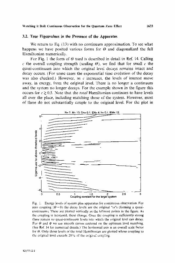
F o r Fig. 1 the form of O used is descr ibed in detai l in Ref. 14. Cal l ing c the overal l coupl ing s t rength (scaling O), we find that for small c the quas i -con t inuum into which the or iginal level decays remains in tac t and decay occurs. ( F o r some cases the exponent ia l t imc evolut ion of the decay was also checked.) However , as c increases, the levels of interest move away, in encrgy, from the or iginal level. There is no longer a con t inuum and the system no longer decays. F o r the example shown in the figure this occurs for c > 0.5. Note that the t o ta l Hami l ton i an cont inues to have levels all over the place, including match ing those of the system. However , mos t of these do not subs tant ia l ly couple to the or iginal level. F o r the plot in

o~

"El

.,Y:

> 0

r

Lu 4

N= 7. M= 13. Cn= 0.1. EN= 4. h= 0.1. EM= 12. i

. . r - - - . . .

~ - " S .

J

Coupling constant for the larger system

Fig. 1. Energy levels of system plus apparatus for continuous observation. For zero coupling (O =0) the decay levels are the original "'o)"s (forming a quasi- continuum). These are plotted vertically as the lcftmost points in the figure. As the coupling is increased, these change, Once the coupling is sutficiently strong there remain no quasi-continuum levels into which the original level can decay, For O and q~ we use smooth curves centered on the optimum level matching. (See Ref. 14 for numerical details,) The horizontal axis is an overall scale lhctor for O. Only those levels of the total Hamiltonian are plotted whose coupling to the original level exceeds 20% of the original coupling,

825/27/I 2-2

1634 Schulman

Fig. 1 only those levels were used for which there was a coupling of at least 20 % of the original coupling, that is, the original "q~."

This result agrees with that reported in Ref. 7. There because of the simplicity of the analytic form we could actually show where the original quasi-continuum had been pushed.

Using the Hamiltonian in Eq. (12) we can also examine the transient behavior of the combined system (decay microsystem plus apparatus). In effect we address the following question. The QZE is often phrased as the observation of a decay system during its quadratic decay interval. In our continuous formulation it is the new exponential decay lifetime that we calculate. What happened to the transient period for the combined system? We now show that indeed the combined system has a transient period, but that it is cut down, essentially by the ratio of the monitored to unmonitored lifetimes.

As shown earlier, an estimate of the duration of the quadratic regime is the jump time, z j, given by vz/rL. Thus we must evaluate--for the combined system--the values of r z and rL. However, this is easy: r z doesn't change, while r L is what Sec. 2 was concerned with, and in particular was denoted z o in that section. [And the calculation of Sec. 2 was related in the present section to the full Hamiltonian of Eq. (12).] To see that Vz is unchanged, recall [ Ref. 6 and Eq. (5) above ] that an alternative phrasing of Zz is

1 2 -- (~'l (H- - (~'l H I~b)) 2 I~b)

~z

essentially the second moment of the Hamiltonian. "~" is the initial undecayed state, in our case a vector with 1 in the first entry, zeros else- where. All that must be done is to square the Hamiltonian in Eq. (12) and look at its 1-1 component. The answer is ~ t ~ , as in Eq. (5). It follows that the duration of the quadratic decay regime scales like the lifetimes.

In Sec. 4 we will further comment on the perspective presented here. The ability to see the QZE as a restructuring of the total Hamiltonian is provided by including the "apparatus" in the Hamiltonian. The insistence that this kind of continuous observation is "only" a matter of changing the system, not seeing the "true" Zeno effect, is in my view an artifact of the traditional but no longer tenable separation of the world into apparatus and system. More on this below.

4. DISCUSSION

Although early formulations of the so-called quantum Zeno effect phrased the phenomenon in terms of repetitive projections on the initial


state of the system, it was soon realized that essentially the same phenomenon could take the form of continuous observations and of observations that varied in time and thereby forced the system to move, rather than stay still.

In the present article we have presented a precise connection between the pulsing time for intermittent observation and the response time for continuous observation. This provides an answer to questions of the form: if I believe the QZE, how can an atom decay if I look at it? The answer is that the response time of your eye (or whatever) is far longer than the times needed to stop that decay via intermittent QZE. (In fact that time is the "jump time" of Ref. 5.) This also explains why observations of quantum jumps (3) did not stop the decay, nor even seriously affect the lifetime.

In establishing this result the apparatus was treated as an ordinary quantum system. This allowed us take an alternative view of the QZE, in which the observer's halting of the decay can be phrased as the system- cum-apparatus ceasing to be an unstable system. This alternative view can sometimes obscure the issue of whether a given observational scheme is or is not an example of the QZE. However, this question is mainly a matter of semantics, and its "answer," whether positive or negative, has no effect on the behavior of the physical systems. In fact, to allay any confusion on this issue it would be better to call the QZE "dominated time evolution," as advocated in Ref. 6.

Yet another reason to prefer the foregoing terminology is the fact that halting change is only one manifestation of the effect. By varying the projections it has long been known that the system may be forced to follow that variation. An example of this, along with a continuous version of such dynamic forcing, is presented in Ref. 14.

A C K N O W L E D G M E N T S

This work is dedicated to Prof. Mikio Namiki on the occasion of his 70th birthday. To some extent it was stimulated by questions he put to one of my collaborators in Ref. 7, Saverio Pascazio. My research is supported in part by the United States National Science Foundation grant PHY 93 16681 and by United States Air Force grant F30602-97-2-0089.

R E F E R E N C E S

1. A. Peres, "Zeno paradox in quantum theory," Am. J. Phys. 48, 931 (1980). 2. E. Joos, "Continuous measurement: Watchdog effect versus golden rule," Phys. Rev. D 29,

1626 (1984).

1636 Schulman

3. J. C. Bergquist, R. G. Hulet, W. M. Itano, and D. J. Wineland, "Observation of quantum jumps in a single atom," Phys. Rev. Lett. 5% 1699 (1986). T. Sauter, W. Neuhauser, R. Blatt, and P. E. Toschek, "Observation of quantum jumps," Phys. Rev. Lett. 5% 1696 (1986). W. Nagourney, J. Sandberg, and H. Dehmelt, "Shelved optical electron amplifier: Observation of quantum jumps," Phys. Rev. Lett. 56, 2797 (1986).

4. L. S. Schulman, "How quick is a quantum jump?," in Proceedings of the Adriatieo Research Conferenee: Tunneling and Its bnplications, D. Mugnai, A. Ranfagni, and L. S. Schulman, eds. (World Scientific, Singapore, 1997).

5. L. S. Schulman, "Observational line broadening and the duration of a quantum jump," J. Phys. A 30, L293 (1997).

6. L. S. Schulman, A. Ranfagni, and D. Mugnai, "Characteristic scales for dominated time evolution," Phys. Scr. 49, 536 (1994).

7. E. Mihokova, S. Pascazio, and L. S. Schulman, "Hindered decay: Quantum Zeno effect through electromagnetic field domination," Phys. Rev. A 56, 25 (1997).

8. H. Nakazato, M. Namiki, and S. Pascazio, "Temporal behavior of quantum mechanical systems," Int. J. Mod. Phys. B 10, 247 (1996).

9. P. K. Kabir, The CP Puzzle: Strange Decays of the Neutral Kaon (Academic, New York, 1968).

10. L. S. Schulman, Time's Arrows and Quantum Measurement (Cambridge University Press, Cambridge, 1997).

11. J. G. Muga, G. W. Wei, and R. F. Snider, "Survival probability for the Yamaguchi Poten- tial," Ann. Phys. 252, 336 (1996).

12. R. B. Griffiths, "Consistent histories and the interpretation of quantum mechanics," J. Stat. Phys. 36, 219 (1984).

13. W. H. Zurek, "Decoherence and the transition from quantum to classical," Phys. Today 36 (October 1991).

14. L. S. Schulman, "Continuous and pulsed observations in the quantum Zeno effect," Phys. Rev. A, to appear.

watching it boil: continuous observation for the quantum zeno effectlschulma/1997watching it... ·...

Documents